Deep Fusion: Efficient Network Training via Pre-trained Initializations

Abstract

In recent years, deep learning has made remarkable progress in a wide range of domains, with a particularly notable impact on natural language processing tasks. One of the challenges associated with training deep neural networks in the context of LLMs is the need for large amounts of computational resources and time. To mitigate this, network growing algorithms offer potential cost savings, but their underlying mechanisms are poorly understood. We present two notable contributions in this paper. First, we present Deep Fusion, an efficient approach to network training that leverages pre-trained initializations of smaller networks. Second, we propose a theoretical framework using backward error analysis to illustrate the dynamics of mid-training network growth. Our experiments show how Deep Fusion is a practical and effective approach that not only accelerates the training process but also reduces computational requirements, maintaining or surpassing traditional training methods’ performance in various NLP tasks and T5 model sizes. Finally, we validate our theoretical framework, which guides the optimal use of Deep Fusion, showing that with carefully optimized training dynamics, it significantly reduces both training time and resource consumption.

1 Introduction

Large language models (LLMs) have significantly advanced the state of the art in various natural language processing tasks, including text generation, translation, summarization, and question answering. However, training these models demands substantial amounts of data and computational resources. As a result, there has been a growing interest in developing efficient training methods to address the challenges associated with the high computational costs and energy consumption during the training process Narayanan et al. (2021).

While some studies Kaplan et al. (2020); Touvron et al. (2023); Zhou et al. (2023) discuss that a balance of data and model size is important, it’s undeniable that larger models often yield better performance Chowdhery et al. (2022). Several experiments and publications have demonstrated that as model size increases, the performance on various natural language processing tasks continues to improve Devlin et al. (2018); Radford et al. (2019); Brown et al. (2020). This trend is evident in the progression of LLMs, such as BERT, GPT-2, GPT-3, and PaLM where each successive generation is larger and achieves better results across a wide range of benchmarks Gu et al. (2021a).

Advancements in LLM efficiency have been driven by a variety of innovative techniques that enable faster training or inference without sacrificing performance. One such approach is model compression, which has been shown to reduce LLM size without significant loss in accuracy Ganesh et al. (2021); Zhang et al. (2022); Kwon et al. (2022). Similarly, adaptive computation time methods have been proposed to dynamically allocate computational resources during LLM training, leading to improved efficiency Graves (2016). Techniques such as layer-wise adaptive rate scaling (LARS) and layer-wise adaptive rate control (LARC) have demonstrated accelerated convergence in LLMs by adapting learning rates on a per-layer basis You et al. (2017b, a). Moreover, recent studies have explored the potential of mixed-precision training, where lower-precision computation is employed during the training process to speed up training and reduce memory requirements Micikevicius et al. (2017). One technique attracting more interest lately is network growing, which is based on increasing transformer size during training. This approach has been shown to speed up training in various studies Shen et al. (2022); Gong et al. (2019); Yao et al. (2023); Gu et al. (2021b); Li et al. (2023), while others report similar or even lower performance compared to standard training methods Kaddour et al. (2023). However, these methods are not well understood and add complexity to the already challenging process of training large language models, both in terms of implementation and correct deployment.

In addition to efficiency, a critical aspect to scale LLM training is distributed training, done by using data or model parallelization. The former splits the training batch across accelerators (e.g., GPUs), while the latter splits the model operations across accelerators so that each accelerator computes part of the model. While data parallelism alone is typically the easiest to implement, it is not well suited for very large models as it needs the whole model to fit in a single accelerator. Model parallelism can be efficient, but it can be more difficult to implement as the dependency between accelerators’ input and outputs can lead to degraded performance.

In our research, we present two novel contributions to emphasize network growing for training efficiency as a primary goal. First, we introduce Deep Fusion, an efficient approach to network training that leverages pre-trained initializations of smaller networks. We employ a fusion operator to combine these smaller networks, promoting wide over-parameterization as a growing mechanism. Deep Fusion serves as a new method to distribute training across accelerators. By enabling the growth from these smaller models, it allows for a modular and efficient distribution of parallel training before the fusion operation, effectively training smaller models for an initial portion of the training process.

Second, we introduce a new theoretical framework based on Backward Error Analysis (BEA) Hairer et al. (2006) to analyze the implicit regularization the optimization process introduces during training right after the fusion operation takes place. BEA has been shown to be an essential analysis tool in many settings, continual-learning Dherin (2023) being of special interest for this work. The main result of the BEA framework is the decomposition of a modified loss into the original loss plus terms that are implicitly minimized during training. When we apply this analysis to Deep Fusion, it becomes clear that the key aspect of our approach lies in a specific interaction component, often referred to as a ‘Lie bracket’ Lee (2022) in differential geometry. This component encapsulates the dynamic interplay between the gradients of the smaller and larger networks, highlighting how they influence and adjust to each other during the first step of the training process.

As we will see throughout the paper, Deep Fusion demonstrates significant reductions in both training time and resource consumption, while maintaining or improving generalization performance.

1.1 Contribution

As part of our research, this paper proposes:

• A method that focuses on initializing large networks from training smaller networks, and employing fusion operators to combine them. This method promotes wide over-parameterization, which leads to improved efficiency in network training.

• An effective framework for the utilization of data and model parallelization techniques, as well as the strategic use of accelerator devices to train models of smaller size. This allows our approach to significantly reduce training time while increasing the performance of the resulting networks.

• A new theoretical framework to analyze dynamically growing wider network algorithms, backed with validation experiments.

• A downstream task evaluation with LLMs, demonstrating its effectiveness and efficiency in various scenarios.

2 Related Work

In line with the lottery ticket hypothesis Frankle and Carbin (2018, 2019), our work shares the following belief: The most commonly used initialization schemes, primarily discovered heuristically Glorot and Bengio (2010); He et al. (2015), are sub-optimal. While there’s some evidence that over-parameterization may not be necessary during training Nakkiran et al. (2020); Belkin et al. (2019), we still believe over-parameterization and a “good” initialization can yield better performance. Thus, we aim to actualize some of the potential that comes from finding a more principled initialization scheme.

From a transfer learning perspective, progressive networks Rusu et al. (2016) grow networks to address the problem of forgetting previous tasks. Another approach, deep model consolidation Zhang et al. (2020), uses a smaller pre-trained model to provide a better initialization for a larger model, which is then fine-tuned on a new task. Network morphism Wei et al. (2016) is another approach that aims to find a larger network by transforming a smaller, pretrained network while preserving the network function during the transformation. This is achieved by expanding the original network with layer-wise operations that preserve input-output behavior.

Similar to our method, staged training Shen et al. (2022) also focuses on network efficiency. This approach involves defining a growth operator while preserving constraints associated with loss and training dynamics. By gradually expanding the model capacity, staged training allows for more efficient training. We argue that preserving training dynamics might not be the most effective approach when it comes to fusion. In fact, it could be counterproductive, and exploring high learning rate cycles could offer a preferable alternative. We validate this theoretically and show it empirically.

BEA has been used in many settings to uncover inductive training biases of various optimizers (e.g. gradient descent Barrett and Dherin (2021), SGD Smith et al. (2021); momentum Ghosh et al. (2023); Adam and RMSProp Cattaneo et al. (2023)), various architectures (e.g., GANs Rosca et al. (2021); diffusion models Gao et al. (2023)), and various training settings like continual-learning Dherin (2023) or distributed and federated learning Barba et al. (2021).

3 Fusion

We start by demonstrating our Fusion operator on two fully connected layers before expanding to T5 transformers.

A generic neural network is a function $f\colon\mathbb{R}^{d}\to\mathbb{R}^{k}$ defined with $r$ layers. A layer $g_{k}:\mathbb{R}^{n}\to\mathbb{R}^{m}$ has weights in layer $k\in[r]$ $w_{k}\in\mathbb{R}^{n\times m}$ and biases being $b_{k}\in\mathbb{R}^{m}$. That is, for each layer $k$ we calculate

$$a_{k}=g_{k}(a_{k-1})=\phi_{k}(a_{k-1}w_{k}+b_{k}),$$ (1)

where $a_{0}=x$ is the input vector, and $\phi_{k}$ is the $k$-th activation function. In what follows, we will omit $a_{k}$ when it is clear from context.

The output of the neural network is defined as the composition of the $r$ layers,

$$f(x)=g_{r}\circ\ldots\circ g_{2}\circ g_{1}(x).$$ (2)

Our Fusion operator $\mathcal{F}$ takes two layers from two different models and generates a new layer by composing their weights and biases. The fused layer has two characteristics:

• Fusion rule: the fused layer maintains the same composition or architecture defined in Eq.1. That is, we do not allow a change in the architecture, but rather a change in the dimensionality of the operations.

• Fusion property: the fused layer calculates the concatenation of the the two original layers that are fused.

The fusion operator ($\mathcal{F}$) is defined as follows. Given two layers with $n$, $n^{\prime}$ inputs and $m$, $m^{\prime}$ outputs,

$$\mathcal{F}_{w} \colon\mathbb{R}^{n\times m}\times\mathbb{R}^{n^{\prime}\times m^{\prime}}\to\mathbb{R}^{(n+n^{\prime})\times(m+m^{\prime})},$$ (3)

$$\mathcal{F}_{b} \colon\mathbb{R}^{m}\times\mathbb{R}^{m^{\prime}}\to\mathbb{R}^{(m+m^{\prime})}.$$ (4)

The Fusion of the weights performed by $\mathcal{F}_{w}$ results in a new matrix where the weights of the layers of the two models are located in the diagonal and the rest is set to zero. Similarly, the new bias is simply the concatenation of the bias of the two layers being fused. So the new fused weight $w^{(f)}$ and new bias $b^{(f)}$ taking the weights of two layers, $w$, $w^{\prime}$, and bias $b$, $b^{\prime}$, respectively is defined as,

$$w^{(f)}=\begin{pmatrix}w&\mathbf{0}\\ \mathbf{0}&w^{\prime}\end{pmatrix},\quad\quad b^{(f)}=[b,b^{\prime}],$$ (5)

where $\mathbf{0}$ is the zero matrix. The output of the fused layer $k$ is defined as,

$$g_{k}^{(f)}= \mathcal{F}(g_{k},g_{k}^{\prime})=\phi_{k}(a_{k-1}^{(f)}\mathcal{F}_{w}(w_{k},w_{k}^{\prime})+\mathcal{F}_{b}(b_{k},b_{k}^{\prime}))$$

$$= \phi_{k}\left([a_{k-1},a_{k-1}^{\prime}]\begin{pmatrix}w_{k}&\mathbf{0}\\ \mathbf{0}&w_{k}^{\prime}\end{pmatrix}+[b_{k},b_{k}^{\prime}]\right)$$

$$= \phi_{k}([a_{k-1}w_{k}+b_{k},a_{k-1}^{\prime}w_{k}^{\prime}+b_{k}^{\prime}])=[g_{k},g_{k}^{\prime}].$$

This means that the result of the Fusion operator on two layers is the concatenation of the outputs, that is $[h_{k},h_{k}^{\prime}]$.

3.1 Deep Fusion and Self Deep Fusion

For two neural networks $f$ and $f^{\prime}$ defined as in Eq. 2, the deep fusion of the two models is defined as follows: We first extend the notation of $\mathcal{F}$ as follows,

$$\mathcal{F}(f,f^{\prime})=\mathcal{F}(g_{r},g_{r}^{\prime})\circ\ldots\circ\mathcal{F}(g_{1},g_{1}^{\prime})([x,x]);$$

And we denote by $\textsc{Avg}(x,y)=(x+y)/2.$ The function that averages two vectors of the same dimension, then the deep fusion is defined as,

$$DF(f,f^{\prime})=\textsc{Avg}(\mathcal{F}(f,f^{\prime})).$$

Intuitively, the deep fused model is maintaining a concatenation of the hidden representations from models $f$ and $f^{\prime}$ (fusion property) throughout the network, and taking the average of their logits.

This means that after the deep fusion operation, the function calculated by the model is equivalent to the function of average ensemble of the two models. However, if we continue training the fused model, the extra parameters added by the zero blocks in the example can start leveraging the hidden representation from the cross model, and potentially lead to better performance.

Deep fusion allows the models to be distributed across multiple GPUs while still taking advantage of the strengths of both data parallelism and model parallelism.

Self deep fusion of a model $f$ is defined as deep fusing the model with itself (that is, $DF(f,f)$). It can be considered a loss preserving growth operation that does not change the network’s predictions to any given input.

3.2 Deep Fusing T5 Transformers

This section describes how to deep fuse two (or more) T5 models Raffel et al. (2019), $f$ and $f^{\prime}$, discussing the particularities of each layer type. Once the fusion is completed, the hidden representation of the newly fused model should be a combination of the two hidden representations from the original models, aligned along the feature dimension axis.

Starting from the bottom layer, the fusion of the embedding layer is trivial. Next, for the multi-head attention, if $f$ has $y$ heads, and $f^{\prime}$ has $y^{\prime}$ heads, then, the fused model will have $y~{}+~{}y^{\prime}$ heads. All projections (query, key, value, attention output) as well as the MLP blocks are treated to prevent leaking information from the wrong hidden representation at initialization.

Note that skip connections and activations are parameter free and do not need further handling. Similarly, the element-wise scaling operation holds a scaling parameter per element in the hidden representation, and thus is trivial to fuse.

Lastly, the fusion of the normalization of the hidden representation between attention and MLP layers proves to be unfeasible. This is due to the fact that it’s not possible to uphold the fusion rule and the fusion property simultaneously. For the normalization layer we either: 1) Preserve the fusion property but break the fusion rule by normalizing the hidden representations of the sub-models individually and then concatenating them; or 2) keep the fusion rule but violate the fusion property by treating the concatenated hidden representation as a single vector for normalization. It’s important to note that the first option requires additional coding beyond parameter initialization, unlike the second option. This dilemma doesn’t occur in self deep fusion.

4 Gradient Flow Bias

In this section, we analyze the inductive bias introduced by network growth using BEA Hairer et al. (2006). The idea behind BEA is to approximate the discrete updates of the optimizer by a continuous gradient flow (described by an ODE called the modified equation) on a modified loss that comprises the original loss and additional terms modelling the inductive biases. For instance, Barrett and Dherin (2021) showed that a single update of SGD follows a gradient flow on the modified (batch) loss $\tilde{L}(\theta)=L(\theta)+\frac{h}{4}\|\nabla_{\theta}L(\theta)\|^{2}$, whose inductive bias is the flatness regularizer $\frac{h}{4}\|\nabla_{\theta}L(\theta)\|^{2}$ depending on the learning rate $h$. More precisely, the modified equation is $\dot{\theta}(t)=-\nabla\tilde{L}(\theta(t)$ and its solution $\tilde{\theta}(h)$ starting at $\theta$ and evaluated at $t=h$ approximates the SGD step $\theta^{\prime}=\theta-h\nabla L(\theta)$ with an error of $\mathcal{O}(h^{3})$. The case of two consecutive updates on the batch losses $L_{1}$ and $L_{2}$ has recently been worked out in Dherin (2023) in the context of continual learning with batches of changing data distribution. In this case, the modified equation is $\dot{\theta}(t)=-\nabla\tilde{L}(\theta(t))-\frac{h}{2}[\nabla L_{1},\nabla L_{2}](\theta(t))$ with modified loss $\tilde{L}(\theta)=L_{1}(\theta)+L_{2}(\theta)+\frac{h}{2}\|\nabla L_{1}(\theta)\|^{2}+\frac{h}{2}\|\nabla L_{2}(\theta)\|^{2}$. In this latter modified equation we see that the Lie bracket $[\nabla L_{1},\nabla L_{2}]$ of the consecutive updates modifies the implicit flatness regularization on both updates. The Lie bracket defined as $[F,G]=(\nabla G)F-(\nabla F)G$ on general vector fields $F,G:\mathbb{R}^{d}\rightarrow\mathbb{R}^{d}$ is an important tool in differential geometry; see Lee (2022) for instance.

We approach the analysis of network growth similarly as a consecutive learning problem. In our new setting, the network before the growth operation is modelled by a small model loss while the model post-growth is modelled by a big model loss. We want to understand the additional inductive bias introduced by the growth step in the optimization. Therefore we are interested in computing the inductive bias generated by the two consecutive optimization steps surrounding the network growth operation. The training of the small model and the large model follow respectively the gradient fields $F(w)=-\nabla_{w}L_{1}(w)$ and $G(w)=-\nabla_{w}L_{2}(w)$. Both vector fields are defined on the parameter space of the large model with $w_{0}=(\theta_{1},\ldots,\theta_{n},\eta=0)$ and subsequent training steps starting from $w=(\theta_{p_{1}},\ldots,\theta_{p_{n}},\eta)$. $\eta$ is the set of parameters in the large model that are not set with the small model and they are set to zero right after fusion.

For $n$ models, immediately after fusion we form parameters $w_{1}$ and its gradient descent update is:

$$w_{1}=w_{0}-h\nabla_{w}L_{1}(w_{0})=w_{0}+hF(w_{0}).$$ (6)

Subsequent steps with vector field $G$ are defined as:

$$w_{2}=w_{1}-h_{B}\nabla_{w}L_{2}(w_{1})=w_{1}+\alpha hG(w_{1}),$$ (7)

where $h_{B}=\alpha h$ is the learning rate for the big model.

The losses $L_{1}(w)$ and $L_{2}(w)$ can be expressed in terms of the small and big models as follows:

$$L_{1}(w) =L\left(\frac{1}{n}\sum_{i=1}^{n}f_{i}(x;\theta_{i}),y\right),$$ (8)

$$L_{2}(w) =L_{B}(w)=L_{B}(\theta_{p_{1}},\ldots,\theta_{p_{n}},\eta),$$ (9)

where $x$ and $y$ are the inputs and reference labels, respectively, and $f_{i}(x;\theta_{i})$ is the output for the $i$-th model with parameters $\theta_{i}$. Note that $L_{1}(w)$ is the loss right after fusion, so all small models are independent but the output is the average operator. Also, for parameters of the form $w_{0}$ with $\eta=0$, we have $L_{1}(w_{0})=L_{2}(w_{0})$.

We present the true modified loss in Theorem 1 and the modified equation in Theorem 2. These theorems suggest that in these network growth settings, the problem does not follow a gradient flow that is some weighted sum of the various losses (before and after the operation); rather, it is biased with the Lie bracket of the gradients’ vector fields. More interestingly, the higher the big network’s learning rate, the more prominent this bias is.

The modified loss in Theorem 1 corresponds with the implicit regularization definition from (Barrett and Dherin, 2021), taking into account the fusion operator.

When the Lie bracket between the two task gradients $[\nabla_{w}L_{1},\nabla_{w}L_{2}]$ is not zero, this may actually interfere with this implicit regularization, potentially creating settings where the second update steers the learning trajectory away from the flatter regions of the first task.

Theorem 1 (Modified loss).

The consecutive gradient updates can be bounded by following the gradient flow on this modified loss:

$$\tilde{L}(w) \leq\frac{1}{n}\sum_{i=1}^{n}L_{S}(\theta_{i})+L_{B}(w)+\frac{h}{4n^{2}}\sum_{i=1}^{n}\lVert\nabla_{\theta_{i}}L_{S}(\theta_{i})\rVert^{2}$$

$$+\frac{h\alpha^{2}}{4}\lVert\nabla_{w}L_{B}(w)\rVert^{2}.$$ (10)

where $L_{S}(\theta_{i})$ is the loss for the $i$-th small model.

For the special case of self-fusion (i.e., the same model is fused with itself), the actual modified loss is,

$$\tilde{L}(w) =L_{S}(\theta)+L_{B}(w)+\frac{h}{4}\lVert\nabla_{\theta}L_{S}(\theta)\rVert^{2}$$

$$+\frac{h\alpha^{2}}{4}\lVert\nabla_{w}L_{B}(w)\rVert^{2}.$$

Theorem 2 (Modified equation).

Consider two consecutive training runs like the ones described above, first a small model, then deep fusion and finally a large model training. The modified equation shadowing the update composition is of the form:

$$\dot{w}(t)=-\nabla_{w}\tilde{L}(w_{t})+\frac{h\alpha}{2}[\nabla_{w}L_{1},\nabla_{w}L_{2}](w_{t})+{\cal O}(h^{2}).$$

Corollary 1.

The larger the learning rate in the big model the more influence of the Lie bracket.

In the coming section, we analyze this bias and understand its structure. Later in the experiment section, we empirically measure its importance.

4.1 Lie Bracket Structure vs the Gradient Loss

In the preceding section, we observed that the Lie bracket serves as a crucial adjustment factor to the gradient difference between the loss of the small model and the fused model. This section examines the Lie bracket from two perspectives. Initially, Lemma 2 confirms that the updated model parameters $\eta$ follow the same gradient updates as the original small model parameters. The Lie bracket’s essential role in fused models becomes evident here; without it, the model updates would be uniform, lacking any additional effects. Subsequently, Lemma 3 illustrates that the Lie bracket ensures the updated parameter directions are the only non-zero components, highlighting the Lie bracket’s significance in refining our algorithm.

For the sake of the analysis, the following discussion assumes a self fusion environment of $n$ models. In the self fusion case, the output of the big model right after fusion is $\hat{y}=\frac{1}{n}\sum_{i=0}^{n}f_{i}(x,\theta_{i})=f(x,\theta)$ given that all models are identical.

Lemma 1 (Scaled gradient).

Let $f$ be a small model with parameters $\theta$. Suppose its loss $L_{S}$ is continuous and that $L_{S}$’s partial derivatives are Lipschitz continuous. When performing self deep fusion $n$ times of $f$, for the first gradient step after fusion, $\nabla_{\theta}L_{B}(\theta,\ldots,\theta,\eta=0)$, we have

$$\nabla_{\theta}L_{B}(\theta,\ldots,\theta,\eta=0)=\frac{1}{n}\nabla_{\theta}L_{S}(\theta).$$

Lemma 2 (Same gradient).

Let $f$ be a small model with parameters $\theta$. When performing self deep fusion $n$ times of $f$, for the first gradient step after fusion for every $\eta_{i}$, we have that

$$\nabla_{\eta_{i}}L_{B}(\theta,\ldots,\theta,\eta=0)=\frac{1}{n}\nabla_{\theta_{j}}L_{S}(\theta),$$

for some $\theta_{j}$ that is a parameter in the same layer.

Lemma 1 and Lemma 2 suggests that the new parameters $\eta$ are updated using a gradient analogous to the combined gradients from the small models. This means that the $\eta$ parameters are updated by concatenating the $\theta_{p_{i}}$ parameters from the small model. Without an implicit Lie bracket term in subsequent gradient steps, the integration of the $\eta$ parameters would be unfeasible.

Lemma 3 (Non-zero Lie bracket).

In self deep fusion, the $[\nabla_{w}L_{1},\nabla_{w}L_{2}]$ has non-zero values only for the parameter dimension $\eta$ that was initialized as zero in the big model.

$$[F,G]=\begin{pmatrix}0\\ \vdots\\ 0\\ (\sum_{i=1}^{n}\nabla_{\theta_{i}}\nabla_{\eta}L_{B}(w))\nabla L_{S}(\theta)\end{pmatrix}$$

In Lemma 3, the analysis requires viewing the problem through the lens of manifolds. Consider $M$ as the manifold of the big model, defined as $M=\{(\theta,\ldots,\theta,\eta):\theta\in\mathbb{R}^{d_{s}},\eta\in\mathbb{R}^{(d_{b}-d_{s})}\}$. The fused model (right after fusion) resides within a smaller submanifold $N\subset M$, where $N=\{(\theta,\ldots,\theta,0):\theta\in\mathbb{R}^{d_{s}}\}$. This lemma demonstrates that the Lie bracket acts as a mathematical tool for understanding the transfer of information between the submanifold $N$ and the ambient manifold $M$.

The Lie bracket $[F,G]$ serves as a correction mechanism that integrates the influence of the submanifold $N$ into the overall system dynamics of $G$. Essentially, the Lie bracket facilitates the exchange of directions between $N$ and $M$.

Corollary 2.

If for the small model $\nabla L_{S}(\theta)$ is close to zero, then the Lie bracket on $N$ is close to zero.

5 Experiments

We begin by training T5 language models on the C4 dataset. The term ‘deep’ will be dropped when context allows.

5.1 Language Models

The aim of this experiment is to establish a better initial checkpoint for a large T5 Raffel et al. (2019) transformer network, referred to as T5-Medium, by using two smaller T5 models, denoted as T5-Small. We present two types of results: fusing two unique small models and fusing one model with itself (self fusion).

We trained the following 4 experiments (see dimensionalities in Table 6 in Appendix B):

1. baseline: T5-Medium from random initialization.

2. fusion-rule: T5-Medium trained from fusing the two T5-Small models while maintaining the fusion rule.

3. fusion-prop: T5-Medium trained from fusing the two T5-Small models while maintaining the fusion property.

4. self-fusion: T5-Medium trained from self fusing a T5-Small model.

Zero matrices in Eq. 5 were substituted with blocks initialized randomly with a low variance. Final results are displayed in Table 1, and Figure 1 shows the evaluation metric curves throughout the training.

Model	Loss @1M	Accuracy @1M
baseline	4.66e+4	66.65 $\pm$ 0.01
fusion-rule	4.61e+4	66.88
fusion-prop	4.53e+4	67.25 $\pm$ 0.03
self-fusion	4.55e+4	67.20 $\pm$ 0.05

Table 1: Performance of different T5-Medium fusion methods at 1 million steps, replicated three times for standard deviation.

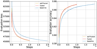
Figure 1: Accuracy and loss on validation data.

The outcomes of our experiments indicate that while it requires extra code changes to the T5 transformer, upholding the fusion property results in superior performance compared to adhering to the fusion rule. Furthermore, we discovered that self fusion yields comparable performance to standard fusion. Significantly, the baseline required an additional 860K steps to achieve the performance level of self fusion. When employing self fusion, training a T5-Medium resulted in an 18% reduction in computation time compared to the baseline.

5.2 Fusion in Stages

We explored staged fusion using T5-S, T5-M, and T5-L architectures (Table 7, Appendix C) and tested various fusion settings depicted in Figure 2.

Figure 2: Settings for final T5-L fusion: yellow signifies fused models, white indicates regular training, and links represent fusion (double link signifies self fusion).

Every model (T5-S, T5-M, T5-L) is trained 1M steps. Table 2 below present the performance of the various models.

Model	Loss @1M steps	Accuracy @1M steps
(1)	4.04e+4	69.89
(2)	3.93e+4	70.45
(3)	3.9e+4	70.56
(4)	3.87e+4	70.74
(5)	3.91e+4	70.57
(6)	3.91e+4	70.47

Table 2: Performance of the various ways of fusing T5-L.

The results show similar performance between fusion and self fusion (settings (3) and (5)). However, repeated self fusion reduces performance, while multiple regular fusions enhance T5-L performance.

Training a model using a single application of self fusion, setting (5), results in a 20% reduction in computation time compared to the standard setting (1).

5.3 Fine Tuning for Down Stream Tasks

We fine-tuned high performing settings from the first experiment together with a baseline on NLP tasks using the GLUE benchmark. We trained two T5-Small models for 500K steps before fusing and self fusing them to create a T5-Medium. We also trained a standalone T5-Medium. These models were fine-tuned at 0 (baseline without pretraining vs fusion without extra training), 250K, 500K, and 1M steps (baseline only). The GLUE average results are shown in Table 3 and Figure 3. The complete results for each task is presented Table 5 in the Appendix.

Model / step	0	250K	500K	1M
baseline	64.07	83.33	84.35	84.74$\pm$0.13
fusion-prop	81.40	84.10	84.86$\pm$0.13	-
self-fusion	81.01	83.71	84.94$\pm$0.2	-
T5-Small	-	-	-	80.28

Table 3: Performance (GLUE average) of the various models on downstream tasks, replicated three times for standard deviation.

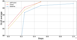
Figure 3: Performance (Glue average - an average over many NLP tasks that score between 0 and 100) of the various models.

Our results indicate that enhancing a pretrained model’s performance may simply require self-fusion before fine-tuning, without further pretraining. For instance, a T5-Small model, trained for 500K steps, when self-fused and fine-tuned, outperforms the same model trained to 1M steps before fine-tuning (81.01 vs 80.28). It is evident that the extra parameters from self-fusion benefit NLP tasks more than extended pretraining.

Next, the results above also suggest that deep fusion can lead to faster training to better performance, when fine-tuning on downstream NLP tasks. However, while in pretrain, the training curves of fusion and self fusion look similar, we can see that for downstream tasks, fusion maintains higher performance throughout until convergence (here, both models converge to similar performance).

Model / time	Fusion	Post fusion	Time	GLUE
baseline	0 steps	1M steps	39.2h	84.74
	0h	39.2h
fusion-prop	500k steps	500k steps	37.9h	84.86
	2$\times$8h	21.9h
self-fusion	500k steps	500k steps	29.9h	84.94
	8h	21.9h

Table 4: Compute time in hours (TPU V3 4x4 topology).

The total compute saving is about 24% TPU time for this configuration as presented in Table 4. Even though we trained for less time, the final performance was slightly better than the baseline.

5.4 Training Dynamics

In this section, our experiments will show how the post-fusion learning rate affects the performance of the learning, as well as the parameters. To understand how the learning rate affects performance, we ran the normal T5 learning rate schedule with various offsets. A positive offset means we start from lower maximal learning rate while a negative offset means we maintain the maximal learning rate for longer before dropping. Figure 4 displays the performance at the extremes (high positive offset vs high negative one). The full tested spectrum of offsets tested appears in Figure 7 in Appendix D.

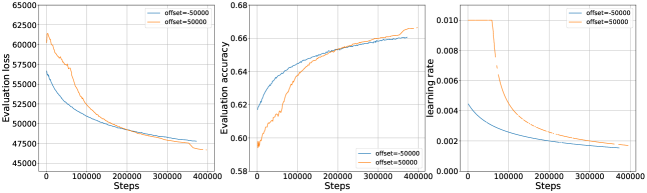
Figure 4: Performance on T5 when applying large offsets to the learning rate schedule.

While it is clear that higher learning rates toward the beginning benefit learning in the long run, we observe they hurt performance at first. This is in line with Section 4 where we show that larger Lie bracket values bias the updates to unlock capacity, but at the short term cost of higher objective loss. Adding a negative offset resulted in better performance, but led to instabilities, and thus the previous experiment did not introduce offsets to the learning rate schedule.

To further understand the drop in performance for low learning rates, we use heat maps to visualize the kernels from the first feed forward layer. Figure 5 shows the kernel when the learning rate is high and low. It is evident that after 400K steps, the parameters initialized to zero were not able to catch up in magnitude with the already optimized ones at expansion point. This observation is further aligned with Section 4 where we note that high learning rates lead to high Lie bracket values, thereby unlocking the potential of the extra parameters.

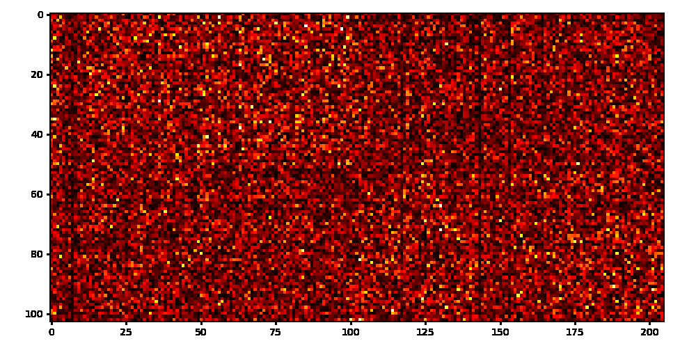
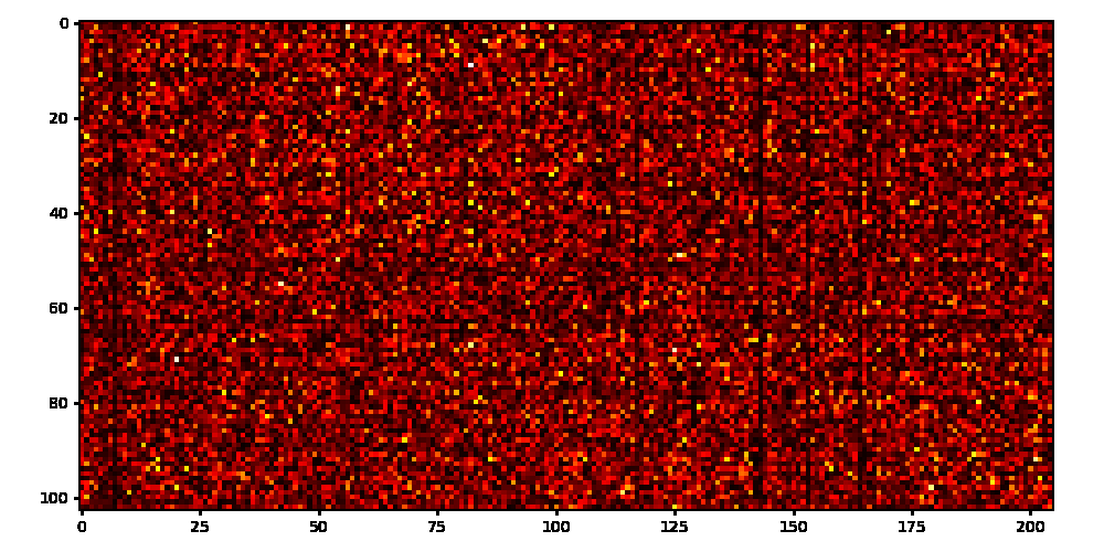
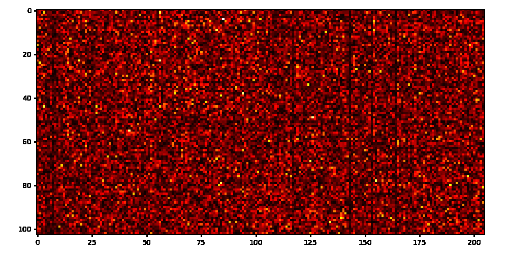
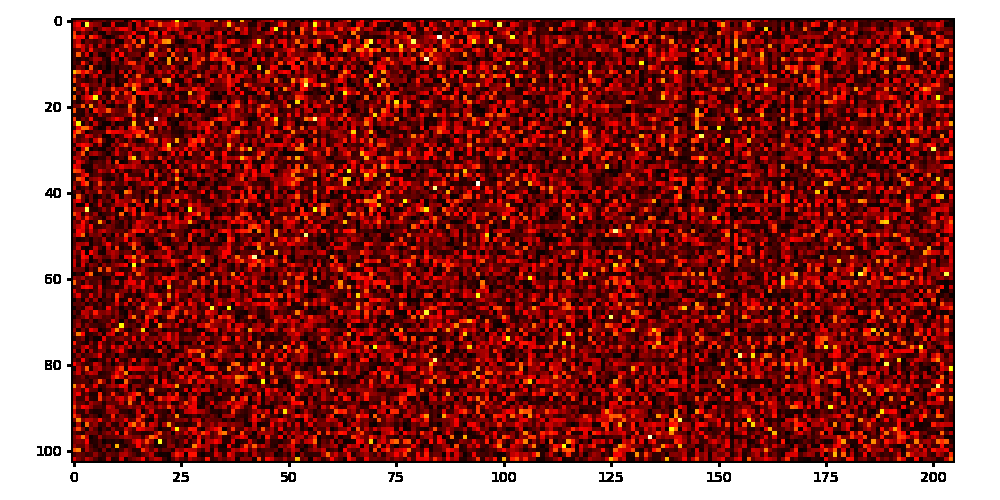
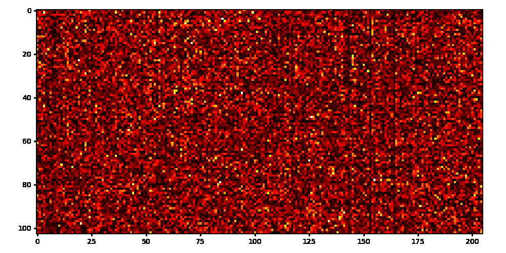
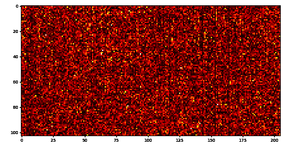
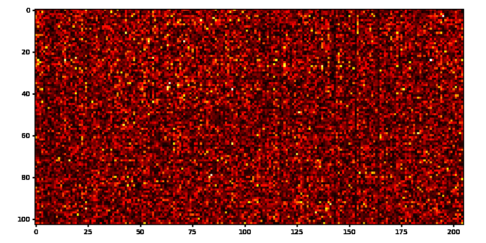
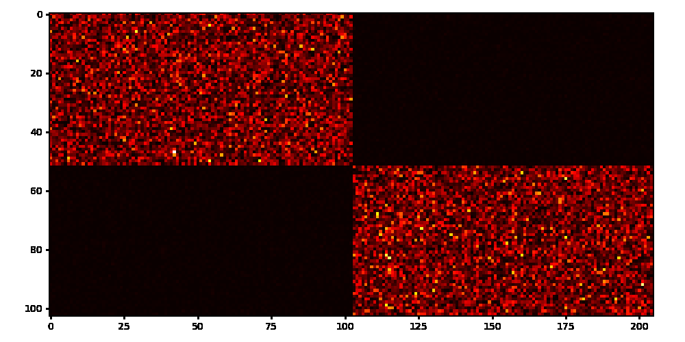
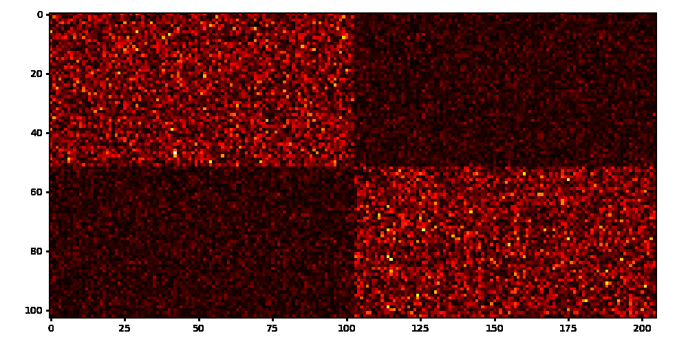
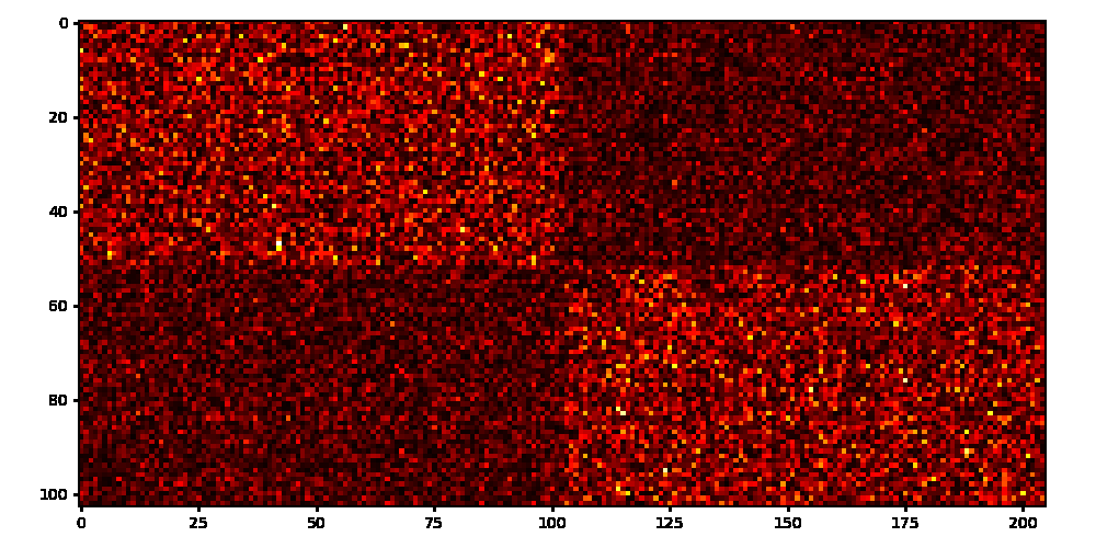
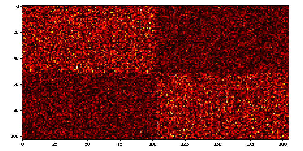
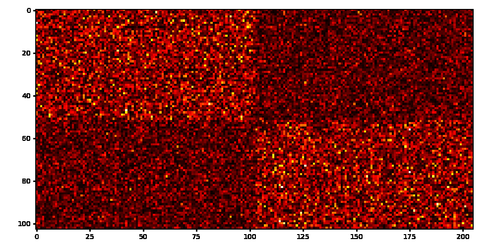
Figure 5: Heat maps of the first layers’ feed forward kernel every 50K steps (left to right till 400K steps training). The upper row is for high learning rates (highly negative offset: -50K), while the lower row is displaying the heat maps for low learning rates (highly positive offset: +50K).

5.5 When to Perform Fusion

Suppose we are given $X$ hours budget of TPU/GPU time, and suppose we would like to grow the network once through training (via self deep fusion), we wanted to answer the question: at which step is it optimal to perform self deep fusion?

We performed experiments training T5-Medium (Table 6 in Appendix B) with various budgets: 50, 60 and 70 hours. The final model was obtained by first training T5-Small and apply self deep fusion at step $x$ during training for various possible steps $x$ (see Figure 6). In the graph, each point represents a different training, where the X-axis represents the step (in 1000s) in which we applied self deep fusion, and the Y-axis represents the final accuracy of the model.

We found that selecting the optimal time to fuse for a given time budget requires some balance.

In particular:

• If the small model has not been trained enough the final fused model will under-perform.

• If the small model is trained and has fully converged, the small model is allotted too much of the budget and the final model shows a slight degradation from optimal.

For the T5-SMALL model, fusing at  500k steps performs well (Figure 6). We note in our experiments the optimal number of steps for the small model was independent of the total budget – a confirmation of the importance of the information transfer when fusing from small to the larger models.

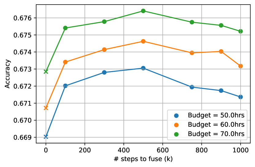
Figure 6: Step to fuse. Displays the final accuracy of the fused model as a function step number when fusion was done (in 1000s). Each color represents a specific total budget allotted to training. The left-most points represent a randomly initialized baseline.

6 Discussion and Conclusion

In this paper, we present a new technique for improving the training process of large models. Our technique, called deep fusion, combines multiple models into a single model that can be trained more efficiently. We demonstrate how model fusion can be used to reduce the restrictions of distributed training, save on overall compute costs, and improve model performance.

Additionally, we introduced a new theoretical framework to illuminate the dynamics of mid-training network growth. This framework offers valuable insights to aid in the design and comprehension of network growing algorithms, easing the potential complexity they introduce when training already intricate large language models.

In our experiments we fused models trained on the same data with identical architectures. While fusion has immediate training advantages, further research is needed to understand the implications and possible applications of fusing models trained on different sources and distinct architectures.

For example, it would be interesting to explore if transfer learning occurs when fusing models trained in different domains. Additional insights could arise by investigating the characteristics of models fused from submodels differing in dimensionality. For instance, one model could be attention-heavy, while another could be MLP-heavy. Finally, one could explore model fusion when the models are trained on different sequence lengths. This could also lead to efficiency improvements, as lower-length models train faster.

Model	Glue avg	COLA Matthew’s	SST acc	MRPC f1	MRPC acc	STS-b pearson	STS-b spearman	qqp acc	qqp f1	MNLI-m	MNLI-mm	QNLI	RTE
baseline 1m	84.74	54.18	94.38	93.17	90.69	89.83	89.75	91.94	89.13	86.77	86.6	92.13	78.34
baseline 1m	84.45	52.95	93.92	93.12	90.44	89.49	89.35	91.94	89.14	86.94	86.58	92.26	77.98
baseline 1m	84.69	53.15	93.81	92.15	88.97	89.06	88.93	92.04	89.24	86.55	86.21	91.69	82.31
Fusion 500k	84.98	53.97	94.27	92.91	90.2	89.68	89.49	92.04	89.36	86.6	86.43	92.39	80.87
Fusion 500k	84.68	54.46	93.81	91.8	88.97	89.44	89.28	91.95	89.13	86.67	86.65	92.11	80.14
Fusion 500k	84.92	53.94	94.5	92.73	89.71	90.62	90.44	92.01	89.23	86.64	86.45	91.56	80.51
Self fusion 500K	84.69	54.58	93.12	92.03	89.22	89.23	89.16	91.81	89.01	86.64	86.68	92.11	80.87
Self fusion 500K	85.19	55.82	93.69	93.1	90.44	89.9	89.73	92.04	89.34	86.8	86.31	92.31	80.87
Self fusion 500K	84.95	58	94.27	92.36	89.71	89.93	89.7	91.96	89.18	86.47	86.4	91.93	77.62

Table 5: Performance (Glue tasks) of the various models on downstream tasks.

Appendix A Proofs

In this appendix, we provide proofs for Theorem 1 and Theorem 2, which are restated below for convenience.

See 1 See 2

Proof.

We are expanding the second part of Eq. 7 using a Taylor series expansion around $w_{0}$:

$$w_{2}= w_{0}+hF(w_{0})+\alpha hG(w_{0}+hF(w_{0}))=$$

$$= w_{0}+h(F(w_{0})+\alpha G(w_{0}))+$$

$$h^{2}\alpha\nabla G(w_{0})F(w_{0})+{\cal O}(h^{3}).$$

We want a modified equation of the form:

$$\dot{w}=H_{0}(w)+hH_{1}(w)+h^{2}H_{2}(w)+\ldots.$$ (11)

The Taylor series expansion of the modified equation solution is:

$$w(h)=w+h\dot{w}+\frac{h^{2}}{2}\nabla\dot{w}\dot{w}+\ldots.$$ (12)

Substituting Eq. 11 into Eq. 12:

$$w(h)= w+h(H_{0}(w)+hH_{1}(w))+$$

$$\frac{h^{2}}{2}H^{\prime}_{0}(w)H_{0}(w)+{\cal O}(h^{3})$$

$$= w+hH_{0}(w)+{\cal O}(h^{3})+$$

$$h^{2}\left(H_{1}(w)+\frac{1}{2}H^{\prime}_{0}(w)H_{0}(w)\right)$$

To have $w_{1}=w(h)$ at first order, we obtain the following condition: $H_{0}(w)=F(w_{0})+\alpha G(w_{0})$ and,

$$H_{1}(w) +\frac{1}{2}H^{\prime}_{0}(w)H_{0}(w)=\alpha\nabla G(w_{0})F(w_{0})$$

$$H_{1}(w) +\frac{1}{2}(\nabla F(w_{0})+\alpha\nabla G(w_{0}))(F(w_{0})+\alpha G(w_{0}))=$$

$$\alpha\nabla G(w_{0})F(w_{0})$$

$$H_{1}(w) =\frac{\alpha}{2}(\nabla G(w_{0})F(w_{0})-\nabla F(w_{0})G(w_{0}))-$$

$$\frac{1}{2}(\nabla F(w_{0})F(w_{0})+\alpha^{2}\nabla G(w_{0})G(w_{0})).$$

Using the definition of $F$ and $G$:

$$\nabla F(w_{0})F(w_{0})= \nabla_{w}(\nabla_{w}L_{1}(w_{0}))\nabla_{w}L_{1}(w_{0})=$$

$$= \frac{\nabla_{w}}{2}\lVert\nabla_{w}L_{1}(w_{0})\rVert^{2}.$$

then,

$$H_{1}(w)= \frac{\alpha}{2}[\nabla_{w}L_{1},\nabla_{w}L_{2}](w_{0})-$$

$$\nabla_{w}\left(\frac{1}{4}\lVert\nabla_{w}L_{1}(w_{0})\rVert^{2}+\frac{\alpha^{2}}{4}\lVert\nabla_{w}L_{2}(w_{0})\rVert^{2}\right).$$

So the continuous modified equation is:

$$\dot{w}(t)= -\nabla_{w}\left(L_{1}(w_{t})+\alpha L_{2}(w_{t})+\frac{h}{4}\lVert\nabla_{w}L_{1}(w_{t})\rVert^{2}+\right.$$

$$\left.\frac{h\alpha^{2}}{4}\lVert\nabla_{w}L_{2}(w_{t})\rVert^{2}\right)+$$

$$\frac{h\alpha}{2}[\nabla_{w}L_{1},\nabla_{w}L_{2}](w_{t})+{\cal O}(h^{2}).$$

We can write the modified loss by substituting $L_{1}(w)$ and $L_{2}(w)$ by their definition using $L_{S}$ and $L_{B}$ to obtain,

$$\tilde{L}(w) =L\left(\frac{1}{n}\sum_{i=1}^{n}f_{i}(x;\theta_{i}),y\right)+L_{B}(w)+$$

$$\frac{h}{4}\lVert\nabla_{\theta_{i}}L\left(\frac{1}{n}\sum_{i=1}^{n}f_{i}(x;\theta_{i}),y\right)\rVert^{2}+$$

$$\frac{h\alpha^{2}}{4}\lVert\nabla_{w}L_{B}(w)\rVert^{2}.$$

Applying Jensen’s inequality to $L\left(\frac{1}{n}\sum_{i=1}^{n}f_{i}(x;\theta_{i}),y\right)<\frac{1}{n}\sum_{i=1}^{n}L(\theta_{i})$, where $L(\theta_{i})=L_{S}(\theta_{i})$ finalizes the proof.

∎

See 1

Proof.

We present the proof for self deep fusion of a model with itself, and the expansion to $n$ copies can be proved in the same manner. First, it is easy to see that when $\theta_{1}=\theta_{2}$ we have

$$\nabla_{\theta_{1}}L_{B}(\theta_{1},\theta_{2},\eta=0)=\nabla_{\theta_{2}}L_{B}(\theta_{1},\theta_{2},\eta=0).$$

This follows immediately in self deep fusion from the symmetry of the network, and the fact that the model is copied twice as is.

Next, we will show that

$$\nabla_{\theta_{2}}L_{S}(\theta_{2}) =\nabla_{\theta_{1}}L_{S}(\theta_{1})=\nabla_{\theta_{1}}L_{B}(\theta_{1},\theta_{2},\eta=0)+$$

$$\nabla_{\theta_{2}}L_{B}(\theta_{1},\theta_{2},\eta=0).$$

To see this note that when $\eta=0$,

$$\nabla_{\theta_{1_{j}}}L_{S}(\theta_{1})=\lim_{\epsilon\rightarrow 0}\frac{L_{S}(\theta_{1}+\mathbf{1}_{j}\cdot\epsilon)-L_{S}(\theta_{1})}{\epsilon}$$

$$=\lim_{\epsilon\rightarrow 0}\frac{L_{B}(\theta_{1}+\mathbf{1}_{j}\cdot\epsilon,\theta_{2}+\mathbf{1}_{j}\cdot\epsilon,\eta)-L_{B}(\theta_{1},\theta_{2},\eta)}{\epsilon}$$

$$=\lim_{\epsilon\rightarrow 0}\frac{1}{\epsilon}\biggl{[}L_{B}(\theta_{1},\theta_{2}+\mathbf{1}_{j}\cdot\epsilon,\eta)+\epsilon\nabla_{\theta_{1_{j}}}L_{B}(\theta_{1},\theta_{2}+\mathbf{1}_{j}\cdot\epsilon,\eta)$$

$$\ \ \ \ \ \ \ \ \ \ +O(\epsilon^{2})-L_{B}(\theta_{1},\theta_{2},\eta)\biggr{]}$$

$$=\lim_{\epsilon\rightarrow 0}\frac{1}{\epsilon}\biggl{[}(L_{B}(\theta_{1},\theta_{2},\eta)+\epsilon\nabla_{\theta_{2_{j}}}L_{B}(\theta_{1},\theta_{2},\eta)+$$

$$\ \ \ \ \ \ \ \ \ \ +\epsilon\nabla_{\theta_{1_{j}}}L_{B}(\theta_{1},\theta_{2}+\mathbf{1}_{j}\cdot\epsilon,\eta)+O(\epsilon^{2})-L_{B}(\theta_{1},\theta_{2},\eta)\biggr{]}$$

$$=\lim_{\epsilon\rightarrow 0}\frac{1}{\epsilon}\biggl{[}L_{B}(\theta_{1},\theta_{2},\eta)+\epsilon\nabla_{\theta_{2_{j}}}L_{B}(\theta_{1},\theta_{2},\eta)+$$

$$\ \ \ \ \ \ \ \ \ \ +\epsilon\nabla_{\theta_{1_{j}}}L_{B}(\theta_{1},\theta_{2},\eta)+O(\epsilon^{2})-L_{B}(\theta_{1},\theta_{2},\eta)\biggr{]}$$

$$=\nabla_{\theta_{1_{j}}}L_{B}(\theta_{1},\theta_{2},\eta)+\nabla_{\theta_{2_{j}}}L_{B}(\theta_{1},\theta_{2},\eta)$$ (13)

In the above, $\mathbf{1}_{j}$ is the unity vector with $j$ being the only non-zero entry, and we use Taylor expansion to move from one line to the other. Additionally, since the functions in question have Lipschitz continuity, then whatever is in the $O(\epsilon^{2})$ can be bounded by a constant times $\epsilon^{2}$. ∎

See 2

Proof.

As before we prove the lemma on fusing the same model twice for simplicity. Extending to $n$ copies can be proved in the same manner. To prove that every parameter in $\eta$ receive the same gradients as some parameter in $\theta$ in the same layer we use the following two observations:

• The hidden representation in every layer is a vector of the form $(y,y)$ for some real number vector $y$ (Fusion Property). This means that the input to every layer is of the form $(y,y)$ for some real number vector $y$.

• Given the above, each parameter in $\eta$ affects the prediction in same way as one of the parameters in $\theta_{i}$, which means adding $\epsilon$ either to that variable, or to the equivalent variable in $\theta_{i}$ has the same effect on the predictions.

More formally, it easy to see that:

$$(y||y)\begin{pmatrix}\theta+\epsilon\mathbf{1}_{i,j}&\mathbf{0}\\ \mathbf{0}&\theta\end{pmatrix}=(y||y)\begin{pmatrix}\theta&\mathbf{0}\\ \mathbf{0}+\epsilon_{1}\mathbf{1}_{i,j}&\theta\end{pmatrix}$$

where $\mathbf{1}_{i,j}$ is a matrix with zeros in every entry except entry ${i,j}$ that is equal to 1.

By definition the gradient for a parameter is the change in loss when applying $\epsilon$ change to the parameter (divided by $\epsilon$). From the above it is easy to see that the gradient for the two parameters is equivalent as they affect the Loss in the same exact way. This together with Lemma 1 concludes the proof. ∎

Corollary 3.

From Lemma 1 and Lemma 2 given a layer with parameters $\theta$, the fused layer gradient looks as follows

$$\nabla_{\theta,\theta,\eta}L_{B}=\begin{pmatrix}\frac{1}{2}\nabla_{\theta}L_{s}&\frac{1}{2}\nabla_{\theta}L_{s}\\ \frac{1}{2}\nabla_{\theta}L_{s}&\frac{1}{2}\nabla_{\theta}L_{s}\end{pmatrix},$$

which concludes the proof.

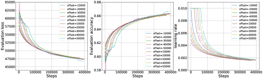
Figure 7: Performance on T5 when applying offsets to the learning rate schedule.

See 3

Proof.

Suppose we are self deep fusing a model $n$ times. Let $M$ be the manifold $M=\{(\theta_{1},\dots,\theta_{n},\eta):\>\theta\in\mathbb{R}^{d_{S}},\eta\in\mathbb{R}^{(d_{b}-d_{s})}\}$; Here $d_{s}$, and $d_{b}$ are the dimension of the small and big models respectively. Since $\theta_{i}=\theta_{j}$ for all $i,j$, the losses $L_{1}$ and $L_{2}$ are of the form,

$$L_{1}(w)=\frac{1}{n}L_{S}(\theta_{1})+\cdots+\frac{1}{n}L_{S}(\theta_{n}),$$

and,

$$L_{2}(w)=L_{B}(\theta_{1},\dots,\theta_{n},\eta).$$

The corresponding vector fields $F(w)$ and $G(w)$ are

$$-\begin{pmatrix}\frac{1}{n}\nabla L_{S}(\theta_{1})\\ \vdots\\ \frac{1}{n}\nabla L_{S}(\theta_{n})\\ 0\end{pmatrix}\ \textrm{and}\ -\begin{pmatrix}\nabla_{\theta_{1}}L_{B}(\theta_{1},\dots,\theta_{n},\eta)\\ \vdots\\ \nabla_{\theta_{n}}L_{B}(\theta_{1},\dots,\theta_{n},\eta)\\ \nabla_{\eta}L_{B}(\theta_{1},\dots,\theta_{n},\eta)\end{pmatrix}.$$

Consider the submanifold $N\subset M$ where

$$N=\{(\theta_{1},\dots,\theta_{n},0):\>\theta\in\mathbb{R}^{d_{S}}\ \mathrm{and}\ \theta_{i}=\theta_{j}\ \forall{i,j}\}.$$

We have the following relation between the small and big model losses on that submanifold (See Lemma 2):

$$\quad\nabla_{\theta_{i}}L_{1}(w)=\nabla_{\theta_{i}}L_{2}(w),$$ (14)

for all $w\in N$. Thus, the vector fields $F$ and $G$ are related as follows:

$$G(w)=-\begin{pmatrix}\frac{1}{n}\nabla L_{S}(\theta_{1})\\ \vdots\\ \frac{1}{n}\nabla L_{S}(\theta_{n})\\ \nabla_{\eta}L_{B}(\theta_{1},\dots,\theta_{n},\eta)\end{pmatrix}=F(w)+g_{\eta}(w)$$

with

$$g_{\eta}=\begin{pmatrix}0\\ \vdots\\ 0\\ -\nabla_{\eta}L_{B}(\theta_{1},\dots,\theta_{n},\eta)\end{pmatrix}$$

This means that the Lie bracket between $F=-\nabla_{w}L_{1}$ and $G=-\nabla_{w}L_{2}$ has the following form on $N$:

$$[F,G] =[F,F+g_{\eta}]$$

$$=[F,F]+[F,g_{\eta}]$$

$$=[F,g_{\eta}]$$

$$=\left[\begin{pmatrix}\nabla L_{S}(\theta_{1})\\ \vdots\\ \nabla L_{S}(\theta_{n})\\ 0\end{pmatrix},\begin{pmatrix}0\\ \vdots\\ 0\\ \nabla_{\eta}L_{B}(\theta_{1},\dots,\theta_{n},\eta)\end{pmatrix}\right]$$

$$=\begin{pmatrix}0\\ \vdots\\ 0\\ (\sum_{i=1}^{n}\nabla_{\theta_{i}}\nabla_{\eta}L_{B}(w))\nabla L_{S}(\theta)\end{pmatrix}$$

which concludes the proof. ∎

Appendix B Model Dimensions for First Experiment

In this appendix, we list the dimension of the T5 transformers used in the first experiment.

Model Name	T5-Small	T5-Medium
embedding dim	512	1024
number of heads	6	12
enc./dec. layers	8	8
head dim	64	64
mlp dimension	1024	2048
number of parameters	77M	242M

Table 6: Dimensions of T5 Small and Medium.

Appendix C Model Dimension for Second Experiment

In this appendix, we list the dimension of the T5 transformers used in the second experiment.

Model Name	T5-S	T5-M	T5-L
embedding dim	512	1024	2048
number of heads	6	12	24
enc./dec. layers	8	8	8
head dim	128	128	128
mlp dimension	1024	2048	4096
number of parameters	95M	317M	1.1B

Table 7: Dimensions of T5-S, T5-M and T5-L.

Appendix D Offsets Experiments Details

In this appendix, we show the performance given various offsets that are applied to the learning rate schedule. The results are inline with the theoretical analysis, meaning the higher the offset (maintaining higher learning rate after growth), the better the final performance. The data is in Figure 7.

References

- Barba et al. [2021] Luis Barba, Martin Jaggi, and Yatin Dandi. Implicit gradient alignment in distributed and federated learning. In AAAI Conference on Artificial Intelligence, AAAI’22, 2021.
- Barrett and Dherin [2021] David G. T. Barrett and Benoit Dherin. Implicit gradient regularization. In ICLR, 2021.
- Belkin et al. [2019] Mikhail Belkin, Daniel Hsu, Siyuan Ma, and Soumik Mandal. Reconciling modern machine-learning practice and the classical bias-variance trade-off. Proceedings of the National Academy of Sciences, 116(32):15849–15854, 2019.
- Brown et al. [2020] Tom B Brown, Benjamin Mann, Nick Ryder, Melanie Subbiah, Jared Kaplan, Prafulla Dhariwal, Arvind Neelakantan, Pranav Shyam, Girish Sastry, Amanda Askell, et al. Language models are few-shot learners. In Advances in Neural Information Processing Systems, pages 14182–14193, 2020.
- Cattaneo et al. [2023] Matias Cattaneo, Jason Klusowski, and Boris Shigida. On the implicit bias of adam. arXiv:2309.00079, 2023.
- Chowdhery et al. [2022] Aakanksha Chowdhery, Sharan Narang, Jacob Devlin, Maarten Bosma, Gaurav Mishra, Adam Roberts, Paul Barham, Hyung Won Chung, Charles Sutton, Sebastian Gehrmann, Parker Schuh, Kensen Shi, Sasha Tsvyashchenko, Joshua Maynez, Abhishek Rao, Parker Barnes, Yi Tay, Noam Shazeer, Vinodkumar Prabhakaran, Emily Reif, Nan Du, Ben Hutchinson, Reiner Pope, James Bradbury, Jacob Austin, Michael Isard, Guy Gur-Ari, Pengcheng Yin, Toju Duke, Anselm Levskaya, Sanjay Ghemawat, Sunipa Dev, Henryk Michalewski, Xavier Garcia, Vedant Misra, Kevin Robinson, Liam Fedus, Denny Zhou, Daphne Ippolito, David Luan, Hyeontaek Lim, Barret Zoph, Alexander Spiridonov, Ryan Sepassi, David Dohan, Shivani Agrawal, Mark Omernick, Andrew M. Dai, Thanumalayan Sankaranarayana Pillai, Marie Pellat, Aitor Lewkowycz, Erica Moreira, Rewon Child, Oleksandr Polozov, Katherine Lee, Zongwei Zhou, Xuezhi Wang, Brennan Saeta, Mark Diaz, Orhan Firat, Michele Catasta, Jason Wei, Kathy Meier-Hellstern, Douglas Eck, Jeff Dean, Slav Petrov, and Noah Fiedel. Palm: Scaling language modeling with pathways, 2022.
- Devlin et al. [2018] Jacob Devlin, Ming-Wei Chang, Kenton Lee, and Kristina Toutanova. Bert: Pre-training of deep bidirectional transformers for language understanding. In Proceedings of the 2019 Conference of the North American Chapter of the Association for Computational Linguistics: Human Language Technologies, pages 4171–4186, 2018.
- Dherin [2023] Benoit Dherin. Implicit biases in multitask and continual learningfrom a backward error analysis perspective. In NeurIPS, Mathematics of Modern Machine Learning Workshop, 2023.
- Frankle and Carbin [2018] Jonathan Frankle and Michael Carbin. The lottery ticket hypothesis: Finding sparse, trainable neural networks. In Proceedings of the International Conference on Learning Representations, 2018.
- Frankle and Carbin [2019] Jonathan Frankle and Michael Carbin. The lottery ticket hypothesis at scale. In arXiv preprint arXiv:1903.01611, 2019.
- Ganesh et al. [2021] Prakhar Ganesh, Yao Chen, Xin Lou, Mohammad Ali Khan, Yin Yang, Hassan Sajjad, Preslav Nakov, Deming Chen, and Marianne Winslett. Compressing Large-Scale Transformer-Based Models: A Case Study on BERT. Transactions of the Association for Computational Linguistics, 9:1061–1080, 09 2021. ISSN 2307-387X. doi: 10.1162/tacl˙a˙00413. URL https://doi.org/10.1162/tacl_a_00413.
- Gao et al. [2023] Yansong Gao, Pan Zhibong, Xin Zhou, Le Kang, and Pratik Chaudhari. Fast diffusion probabilistic model sapling through the lens of backward error analysis. arXiv:2304.11446, 2023.
- Ghosh et al. [2023] Avrajit Ghosh, He Lyu, Xitong Zhang, and Rongrong Wang. Implicit regularization in heavy-ball momentum accelerated stochastic gradient descent. ICLR, 2023.
- Glorot and Bengio [2010] Xavier Glorot and Yoshua Bengio. Understanding the difficulty of training deep feedforward neural networks. In Proceedings of the Thirteenth International Conference on Artificial Intelligence and Statistics, pages 249–256, 2010.
- Gong et al. [2019] L. Gong, D. He, Z. Li, T. Qin, L. Wang, and T. Liu. Efficient training of bert by progressively stacking. In ICML 2019, 2019. URL https://proceedings.mlr.press/v97/gong19a.html.
- Graves [2016] Alex Graves. Adaptive computation time for recurrent neural networks. In Proceedings of the International Conference on Learning Representations, 2016.
- Gu et al. [2021a] Jiatao Gu, Jianqiang Hu, Tong Zhao, Ying Lin, Xiuying Cheng, Lijun Wang, and Xiang Wan. Palm: Pre-training an autoencoding and autoregressive language model for context-conditioned generation. In Proceedings of the 2021 Conference on Empirical Methods in Natural Language Processing, pages 2643–2662, 2021a.
- Gu et al. [2021b] Xiaotao Gu, Liyuan Liu, Hongkun Yu, Jing Li, Chen Chen, and Jiawei Han. On the transformer growth for progressive bert training. In In Proceedings of the 2021 Conference of the North American Chapter of the Association for Computational Linguistics: Human Language Technologies, page 5174–5180, 2021b.
- Hairer et al. [2006] Ernst Hairer, Christian Lubich, and Gerhard Wanner. Geometric numerical integration, volume 31 of Springer Series in Computational Mathematics. Springer-Verlag, Berlin, second edition, 2006. ISBN 3-540-30663-3; 978-3-540-30663-4. Structure-preserving algorithms for ordinary differential equations.
- He et al. [2015] Kaiming He, Xiangyu Zhang, Shaoqing Ren, and Jian Sun. Delving deep into rectifiers: Surpassing human-level performance on imagenet classification. In Proceedings of the IEEE International Conference on Computer Vision, pages 1026–1034, 2015.
- Kaddour et al. [2023] Jean Kaddour, Oscar Key, Piotr Nawrot, Pasquale Minervini, and Matt J. Kusner. No train no gain: Revisiting efficient training algorithms for transformer-based language models. In Neurips 2023, 2023. URL https://arxiv.org/pdf/2307.06440.pdf.
- Kaplan et al. [2020] Jared Kaplan, Sam McCandlish, Tom Henighan, Tom B Brown, Benjamin Chess, Rewon Child, Scott Gray, Alec Radford, Jeffrey Wu, and Dario Amodei. Scaling laws for neural language models. arXiv preprint arXiv:2001.08361, 2020.
- Kwon et al. [2022] Woosuk Kwon, Sehoon Kim, Michael W. Mahoney, Joseph Hassoun, Kurt Keutzer, and Amir Gholami. A fast post-training pruning framework for transformers. In Alice H. Oh, Alekh Agarwal, Danielle Belgrave, and Kyunghyun Cho, editors, Advances in Neural Information Processing Systems, 2022. URL https://openreview.net/forum?id=0GRBKLBjJE.
- Lee [2022] John Lee. Introduction to smooth manifolds. In Springer, 2022.
- Li et al. [2023] Xiang Li, Yiqun Yao, Xin Jiang, Xuezhi Fang, Xuying Meng, Siqi Fan, Peng Han, Jing Li, Li Du, Bowen Qin, Zheng Zhang, Aixin Sun, and Yequan Wang. Flm-101b: An open llm and how to train it with $100k budget. In Arxiv, 2023. URL https://arxiv.org/pdf/2309.03852.pdf.
- Micikevicius et al. [2017] Paulius Micikevicius, Sharan Narang, Jonah Alben, Gregory Diamos, Erich Elsen, David Garcia, Boris Ginsburg, Michael Houston, Oleksii Kuchaiev, Ganesh Venkatesh, et al. Mixed precision training. In Proceedings of the International Conference on Learning Representations, 2017.
- Nakkiran et al. [2020] Preetum Nakkiran, Gal Kaplun, Yamini Bansal, Tristan Yang, Boaz Barak, and Ilya Sutskever. Deep double descent: Where bigger models and more data hurt. In Proceedings of the International Conference on Learning Representations, 2020.
- Narayanan et al. [2021] Deepak Narayanan, Mohammad Shoeybi, Jared Casper, Patrick LeGresley, Mostofa Patwary, Vijay Korthikanti, Dmitri Vainbrand, Prethvi Kashinkunti, Julie Bernauer, Bryan Catanzaro, Amar Phanishayee, and Matei Zaharia. Efficient large-scale language model training on gpu clusters using megatron-lm. In Proceedings of the International Conference for High Performance Computing, Networking, Storage and Analysis, SC ’21, New York, NY, USA, 2021. Association for Computing Machinery. ISBN 9781450384421. doi: 10.1145/3458817.3476209. URL https://doi.org/10.1145/3458817.3476209.
- Radford et al. [2019] Alec Radford, Karthik Narasimhan, Tim Salimans, and Ilya Sutskever. Language models are unsupervised multitask learners. In OpenAI Blog, 2019.
- Raffel et al. [2019] Colin Raffel, Noam Shazeer, Adam Roberts, Katherine Lee, Sharan Narang, Michael Matena, Yanqi Zhou, Wei Li, and Peter J. Liu. Exploring the limits of transfer learning with a unified text-to-text transformer. CoRR, 2019. URL http://arxiv.org/abs/1910.10683.
- Rosca et al. [2021] Mihaela Rosca, Yan Wu, Benoit Dherin, and David G.T. Barrett. Discretization drift in two-player games. In ICML, 2021.
- Rusu et al. [2016] Andrei A Rusu, Neil C Rabinowitz, Guillaume Desjardins, Hubert Soyer, James Kirkpatrick, Koray Kavukcuoglu, Razvan Pascanu, and Raia Hadsell. Progressive neural networks. In Proceedings of the 30th International Conference on Neural Information Processing Systems, pages 2212–2220, 2016.
- Shen et al. [2022] Sheng Shen, Pete Walsh, Kurt Keutzer, Jesse Dodge, Matthew Peters, and Iz Beltagy. Staged training for transformer language models. In Kamalika Chaudhuri, Stefanie Jegelka, Le Song, Csaba Szepesvari, Gang Niu, and Sivan Sabato, editors, Proceedings of the 39th International Conference on Machine Learning, volume 162 of Proceedings of Machine Learning Research, pages 19893–19908. PMLR, 17–23 Jul 2022. URL https://proceedings.mlr.press/v162/shen22f.html.
- Smith et al. [2021] Samuel L Smith, Benoit Dherin, David G.T. Barrett, and Soham De. On the origin of implicit regularization in stochastic gradient descent. In ICLR, 2021.
- Touvron et al. [2023] Hugo Touvron, Thibaut Lavril, Gautier Izacard, Xavier Martinet, Marie-Anne Lachaux, Timothée Lacroix, Baptiste Rozière, Naman Goyal, Eric Hambro, Faisal Azhar, Aurelien Rodriguez, Armand Joulin, Edouard Grave, and Guillaume Lample. Llama: Open and efficient foundation language models, 2023.
- Wei et al. [2016] Chen Wei, Haoyu Wang, Yongyang Rui, and Changqing Chen. Network morphism. In Proceedings of the 33rd International Conference on International Conference on Machine Learning, pages 2662–2671, 2016.
- Yao et al. [2023] Yiqun Yao, Zheng Zhang, Jing Li, and Yequan Wang. 2x faster language model pre-training via masked structural growth. In Arxiv, 2023. URL https://arxiv.org/pdf/2305.02869.pdf.
- You et al. [2017a] Yang You, Yaroslav Bulatov, Igor Gitman, and Andrej Risteski. Large batch training of convolutional networks. In arXiv preprint arXiv:1708.03888, 2017a.
- You et al. [2017b] Yang You, Igor Gitman, and Boris Ginsburg. Scaling sgd batch size to 32k for imagenet training. In Deep Learning Scaling is Predictable, Empirically, page 13, 2017b.
- Zhang et al. [2020] Junting Zhang, Jie Zhang, Shalini Ghosh, Dawei Li, Serafettin Tasci, Larry Heck, Heming Zhang, and C. C. Jay Kuo. Class-incremental learning via deep model consolidation, 2020.
- Zhang et al. [2022] Qingru Zhang, Simiao Zuo, Chen Liang, Alexander Bukharin, Pengcheng He, Weizhu Chen, and Tuo Zhao. Platon: Pruning large transformer models with upper confidence bound of weight importance, 2022.
- Zhou et al. [2023] Chunting Zhou, Pengfei Liu, Puxin Xu, Srini Iyer, Jiao Sun, Yuning Mao, Xuezhe Ma, Avia Efrat, Ping Yu, Lili Yu, Susan Zhang, Gargi Ghosh, Mike Lewis, Luke Zettlemoyer, and Omer Levy. Lima: Less is more for alignment, 2023.