Unexplainable Explanations: Towards Interpreting tSNE and UMAP Embeddings

Abstract

It has become standard to explain neural network latent spaces with attraction/repulsion dimensionality reduction (ARDR) methods like tSNE and UMAP. This relies on the premise that structure in the 2D representation is consistent with the structure in the model’s latent space. However, this is an unproven assumption – we are unaware of any convergence guarantees for ARDR algorithms. We work on closing this question by relating ARDR methods to classical dimensionality reduction techniques. Specifically, we show that one can fully recover a PCA embedding by applying attractions and repulsions onto a randomly initialized dataset. We also show that, with a small change, Locally Linear Embeddings (LLE) can reproduce ARDR embeddings. Finally, we formalize a series of conjectures that, if true, would allow one to attribute structure in the 2D embedding back to the input distribution.

1 Introduction

The modern machine learning engineer has no doubt used a neural network without fully knowing what the model chose to prioritize in the data. Indeed, deep learning models are known to take shortcuts, focusing on spurious correlations rather semantic-level features in the data. Thus, the field of Explainable AI (XAI) has risen to prominence to help analyze machine learning models and align the user’s intuition with the model’s feature extraction process.

The first step towards interpreting what a network has learned is to inspect the distributions in its feature space. Since deep learning embeddings are too high-dimensional to interpret on their own, it is common to perform dimensionality reduction (DR) to get the embedding vectors into 2D. To this end, tSNE [1] and UMAP [2] have become the de-facto tool for visualizing learned representations due to their attractive properties – they are unsupervised, fast to optimize and produce 2D distributions with neatly separated clusters. In fact, it has become almost standard to show that a feature extractor works as intended by plotting its embeddings with tSNE or UMAP; a (very) non-exhaustive list of examples can be found in [3, 4, 5, 6, 7, 8, 9, 10, 11, 12, 13, 14, 15, 16, 17, 18, 19, 20, 21, 22, 23, 24, 25, 26, 27, 28, 29, 30, 31, 32, 33, 34, 35, 36, 37, 38, 39, 40, 41, 42, 43, 44, 45, 46, 47].

However, despite tSNE and UMAP giving intepretable embeddings and being used for network explainability, they themselves are not well understood. For example, [48] showed that UMAP’s implementation does not optimize the intended loss function, implying that the theoretical motivation may not hold in practice. Furthermore, it has been a point of active research to investigate how the loss functions, gradient descent strategies, and heuristic accelerations alter the structure of tSNE and UMAP embeddings [49, 50, 51, 52, 53], with many works suggesting that the common wisdom surrounding tSNE and UMAP may not hold. Thus, it is unclear whether conclusions drawn from the 2D embeddings can be carried over to the neural network’s learned representation. Essentially, the community is trying to solve an explainability problem with a tool that has a well-studied explainability problem.

Luckily, modern methods like tSNE and UMAP exist in a landscape of otherwise well-understood DR techniques. For example, it is known that Principal Component Analysis (PCA) maximally preserves variance from the input distribution. Thus, given a PCA embedding, one can confidently attribute structure back to the original dataset. Similar conclusions can be drawn for other classic DR techniques such as Locally Linear Embeddings (LLE) [54, 55], ISOMAP [56], Laplacian Eigenmaps [57], and Multi-Dimensional Scaling (MDS) [58], to name a few. Importantly, their explainability is a direct consequence of the convergence guarantees of each algorithm. Unfortunately, these do not provide the intuitive separation that deep learning practitioners want and are therefore not as popular for visualizing latent spaces. Thus, the field has been inadvertently partitioned: DR methods are either well-understood or are useful for deep learning explainability, but not both.

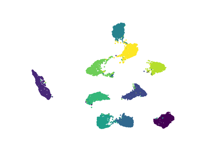
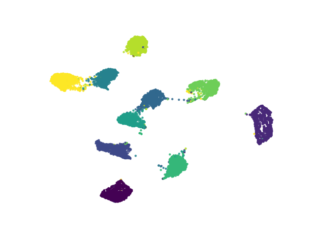
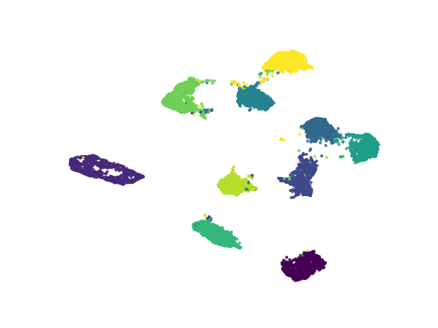
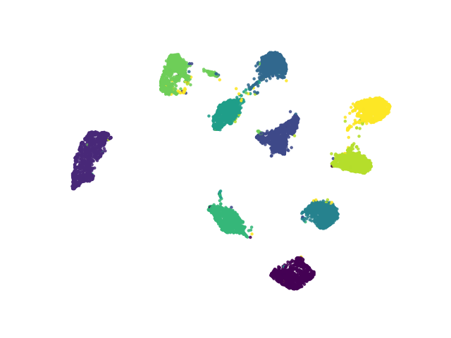
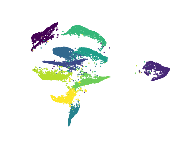
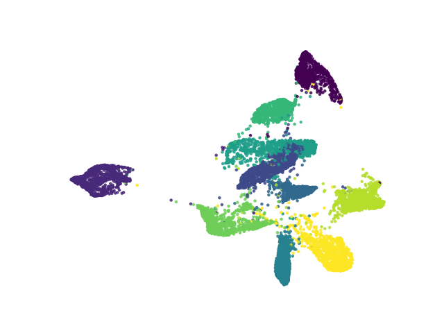
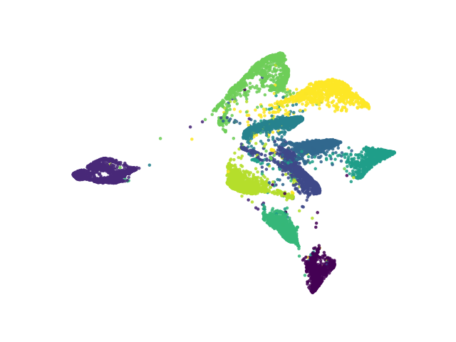
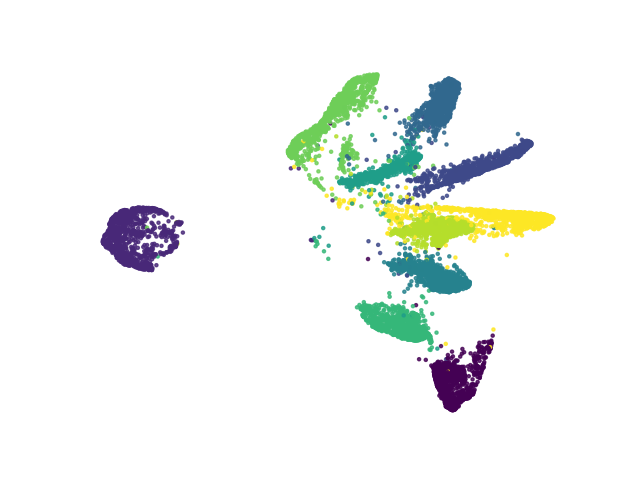
Figure 1: UMAP/tSNE (top/bottom) embeddings of the last conv. layer of VGG11 [59] on MNIST mid-training. 3 columns have $>\!\!90\%$ accuracy while one has $72\%$ accuracy. We purposefully omit which column corresponds to the low-accuracy latent space.

1.1 Our Contributions

Our work aims to bridge the gap between these two types of methods. We start by defining a framework for representing methods such as PCA and LLE in the tSNE/UMAP setting. Specifically, we show that one can provably obtain PCA embeddings by performing attractions and repulsions between points and that this is robust to fast low-rank approximations. Furthermore, we show that minimizing the PCA and LLE objective functions with the UMAP kernel on the 2D embedding gives similar gradients as those found in tSNE/UMAP. We verify this experimentally by showing that minimizing the LLE objective with this kernel gives comparable embeddings to tSNE/UMAP. Thus, we show that classical methods are reproducible in the modern DR framework.

This naturally leads us to ask whether the relationship goes the other way. Specifically, we conjecture that the tSNE/UMAP gradient descent heuristics minimize the LLE objective with two kernels. If this holds true, it would suggest that one does not require gradient descent to find an embedding that is provably similar to those obtained by tSNE/UMAP. In this sense, we hope to facilitate future work towards the open question: “Which properties in the tSNE/UMAP embedding guarantee structure in the original dataset?” We identify that the crux of this question lies in the poorly-studied dynamics imposed by the kernel added on the embedding and discuss opportunities for future work therein.

2 Related Work

There has been a significant attempt in recent years to explain deep learning models’ learned representations. Some methods attempt to explain a model’s decision-making using specific data examples, for instance through saliency maps [60, 61, 62] or counterfactual explanations [63, 64]. Other approaches focus on visualizing some aspect of the network itself, such as feature activations, convolution filters [62], and the feature vectors by finding neighbors [65], or embedding them into 2D, as we will discuss below.

For the rest of the paper we will refer to the class of gradient-based dimensionality reduction techniques that includes tSNE and UMAP as Attraction/Repulsion DR (ARDR) methods. The common theme among these is that they define notions of similarity in the input $\mathbf{X}$ and the embedding $\mathbf{Y}$ and minimize a loss function by attracting points in $\mathbf{Y}$ that should be similar and repelling points that should be dissimilar. A non-exhaustive list of methods includes tSNE [1, 66], UMAP [2], ForceAtlas2 [67], LargeVis [68] and PacMAP [50]. Similar methods such as TriMAP [69] discuss this in the context of triplets but we note that the underlying schema of gradient descent by attractions and repulsions remains the same.

Despite the popularity of ARDR methods, there has been a recent wave of literature that disputes the common wisdom surrounding them. We recommend [70] to increase intuition regarding how tSNE’s hyperparameters affect one’s ability to relate the structures in the input and 2D embedding. We note that UMAP has similar issues to those raised for tSNE in [70]. For more rigorous analysis that dispels myths regarding ARDR methods, [49] showed that UMAP’s seemingly stronger attractions are a result of the sampling strategy rather than the topological properties of the algorithms. This was followed by [48], which noted the surprising fact that UMAP does not actually optimize its stated loss function due to the heuristics it employs during gradient descent. Further analysis of ARDR loss functions can be found in [50, 51]. We note that [52] found that one can replace the KL divergence in UMAP by the sum of squared errors without impacting the embeddings in practice. Furthermore, the manifold learning intuitions regarding ARDR methods were questioned in [71, 69, 53], where it was shown that it is unclear whether tSNE and UMAP are preserving local/global structure in the expected manner. Lastly, other works have sought to unify tSNE and UMAP by verifying that they are effectively identical up to a hyperparameter [52] and can both be reproduced within the contrastive learning framework [72].

We are less aware of literature comparing classical DR techniques to the modern wave of gradient-based ones. [51] defines a framework to unify classical and modern DR methods, but the generality of the approach makes it difficult to make direct claims regarding the connection between methods like PCA and UMAP. Furthermore, tSNE does not fit into their framework in a natural manner. Indeed, the reference most similar to ours is [53], where the authors analyze the manifold-learning properties of popular DR approaches towards the goal of improved explainability. They study how well various DR techniques preserve locality via a novel measure and show that (1) tSNE/UMAP preserve locality better than most classical methods, and (2) that tSNE/UMAP distort the Euclidean relationships more strongly than other DR methods. We share the authors’ surprise regarding the lack of literature on explainable DR methods since dimensionality reduction is a natural step towards gathering intuition on learned representations.

We approach the question of explainability from the other direction. Whereas [53] studies the experimental properties of embeddings obtained by modern and classical methods, we instead relate their theoretical foundations. Specifically, Section 3 provides background on PCA, LLE, and ARDR methods, after which Sections 4 and  5 show how to interpret classical methods in terms of attractions and repulsions between points. We conclude by motivating conjectures and open questions in 6.

3 Preliminaries

3.1 Principal Component Analysis (PCA)

Likely the most famous dimensionality reduction algorithm, PCA finds the orthogonal basis in $\mathbb{R}^{n\times d}$ that maximally preserves the variance in the centered dataset [73]. Let $\mathbf{C}\mathbf{X}=\mathbf{U}_{X}\mathbf{\Sigma}_{X}\mathbf{V}_{X}^{\top}$ be the singular value decomposition (SVD) of the centered dataset, where $\mathbf{C}=\mathbf{I}-\frac{1}{n}\mathbf{J}$ is the centering matrix with $\mathbf{J}$ the all-1 matrix. This gives us an expression for the positive semidefinite (psd) Gram matrix $\mathbf{C}\mathbf{G}_{X}\mathbf{C}=\mathbf{C}\mathbf{X}\mathbf{X}^{\top}\mathbf{C}=\mathbf{U}_{X}\mathbf{\Sigma}_{X}^{2}\mathbf{U}_{X}^{\top}$. The principal components of $\mathbf{C}\mathbf{X}$ are defined as $\mathbf{U}_{X}\mathbf{\Sigma}_{X}$ can therefore be found via eigen-decomposition on $\mathbf{C}\mathbf{G}_{X}\mathbf{C}$.

This has a natural extension to kernel methods [74]. Suppose that the kernel function $k_{x}(x_{i},x_{j})=\langle\phi(x_{i}),\phi(x_{j})\rangle$ corresponds to an inner product space. Then the kernel matrix $\left[\mathbf{K}\right]_{ij}=k(x_{i},x_{j})$ is a psd Gram matrix for the space defined by $\phi$ and admits an equivalent procedure for finding principal components as traditional PCA.

3.2 Locally Linear Embedding (LLE)

Since PCA embeddings are obtained via linear projection operations, one can think of them as preserving large distances in the dataset. On the other hand, LLE preserves local neighborhoods by finding the $\mathbf{Y}$ that maximally recreates linear combinations of nearest-neighbors in $\mathbf{X}$. Assume that we have the $k$-nearest-neighbor graph on $\mathbf{X}$ and let $K_{i}=\{e_{i1},\cdots e_{ik}\}$ represent the indices of $x_{i}$’s $k$ nearest neighbors in $\mathbf{X}$. LLE then proceeds by finding the $\mathbf{W}\in\mathbb{R}^{n\times n}$ such that

$$\sum_{i}||x_{i}-\sum_{j\in K_{i}}w_{ij}x_{j}||_{2}^{2}=||\mathbf{X}-\mathbf{W}\mathbf{X}||_{F}^{2}=||(\mathbf{I}-\mathbf{W})\mathbf{X}||_{F}^{2}$$

is minimized under the constraint $\sum_{j\in K_{i}}w_{ij}=1$ for all $i$. That is, we find the weights such that each point $x_{i}$ is represented as a linear combination of its neighbors. This implies that the $i$-th row of $\mathbf{W}$ must be zero on the indices $l$ where $x_{l}$ is not $x_{i}$’s nearest neighbor. It can be shown that such a $\mathbf{W}$ always exists and each row can be found by solving an eigenproblem [54, 55].

Having found the $\mathbf{W}$ that represents local neighborhood relationships in $\mathbf{X}$, step 2 of LLE then finds the $\mathbf{Y}\in\mathbb{R}^{n\times d}$ such that

$$\sum_{i}||y_{i}-\sum_{j\in K_{i}}w_{ij}y_{ij}||_{2}^{2}=||\mathbf{Y}-\mathbf{W}\mathbf{Y}||_{F}^{2}$$

is minimized, subject to the constraint that the columns of $\mathbf{Y}$ form an orthogonal basis, i.e. $\frac{1}{n}\mathbf{Y}^{\top}\mathbf{Y}=\mathbf{I}$. The embedding $\mathbf{Y}$ is given by the eigenvectors of $\mathbf{M}=(\mathbf{I}-\mathbf{W})^{\top}(\mathbf{I}-\mathbf{W})$ that correspond to the smallest $d$ positive eigenvalues (Derivation in B.1).

LLE can again be combined with kernels on $\mathbf{X}$ and $\mathbf{Y}$ to perform more sophisticated similarity calculations [55]. Let $\mathbf{K}_{X}$ be defined as in Section 3.1 and let $k_{y}(y_{i},y_{j})=\langle\psi(y_{i}),\psi(y_{j})\rangle$ be a psd kernel that defines a corresponding $\mathbf{K}_{Y}\in\mathbb{R}^{n\times n}$ with $[\mathbf{K}_{Y}]_{ij}=k_{y}(y_{i},y_{j})$. Then we can define the objective function during the first step as finding the $\mathbf{W}$ that minimizes $\text{Tr}\left((\mathbf{I}-\mathbf{W})\mathbf{K}_{X}(\mathbf{I}-\mathbf{W})^{\top}\right)$ such that $\sum_{j}w_{ij}=1$ for all $i$. Similarly, the second step under a kernel function $\mathbf{K}_{Y}$ seeks the $\mathbf{Y}$ such that $\text{Tr}\left((\mathbf{I}-\mathbf{W})\mathbf{K}_{Y}(\mathbf{I}-\mathbf{W})^{\top}\right)$ is minimized.

3.3 Gradient Dimensionality Reduction Methods

We now switch gears from the directly solvable methods to the gradient-based ones which have risen to prominence in the last decade. This includes algorithms such as UMAP, tSNE, LargeVis, and PacMAP, just to name a few.

3.3.1 In theory

ARDR methods

Assume that we are given an input $\mathbf{X}\in\mathbb{R}^{n\times D}$, a randomly initialized embedding $\mathbf{Y}\in\mathbb{R}^{n\times d}$ and two psd kernel functions $k_{x}(x_{i},x_{j})=\langle\phi(x_{i}),\phi(x_{j})\rangle$ and $k_{y}(y_{i},y_{j})=\langle\psi(y_{i}),\psi(y_{j})\rangle$. These then define psd matrices $\mathbf{K}_{X},\mathbf{K}_{Y}\in\mathbb{R}^{n\times n}$, where each $(i,j)$-th entry represents the set of per-point similarities in $\mathbf{X}$ and $\mathbf{Y}$ respectively. Given this setup, the goal of gradient-based DR methods is to find the embedding $\mathbf{Y}$ such that $\mathbf{K}_{Y}$ is maximally similar to $\mathbf{K}_{X}$ with respect to some matrix-wise loss function.

For the remainder of this section, the reader can assume that $k_{x}$ is the exponential RBF kernel and $k_{y}$ is the quadratic Cauchy kernel; these are the common choices across ARDR methods. However, we note that the upcoming generalizations only require that $k_{y}$ be a function of the squared Euclidean distance. We will write $k_{y}(||y_{i}-y_{j}||_{2}^{2})$ when emphasizing this point.

Since the kernels are usually chosen such that $k_{x}$ and $k_{y}$ are necessarily in $[0,1]$, the matrices can be treated as probability distributions. Thus, the question of how well $\mathbf{K}_{Y}$ represents $\mathbf{K}_{X}$ is traditionally quantified using the KL-divergence $KL(\mathbf{K}_{X}||\mathbf{K}_{Y})$. For example, tSNE and UMAP state the following loss functions

$$\mathcal{L}_{tSNE}(\mathbf{X},\mathbf{Y}) =\sum^{n}_{\begin{subarray}{c}i,j=1\\ i\neq j\end{subarray}}k_{x}(x_{i},x_{j})\log\left(\frac{k_{x}(x_{i},x_{j})}{k_{y}(y_{i},y_{j})}\right)$$ (1)

$$\mathcal{L}_{UMAP}(\mathbf{X},\mathbf{Y}) =\sum^{n}_{\begin{subarray}{c}i,j=1\\ i\neq j\end{subarray}}k_{x}(x_{i},x_{j})\log\left(\frac{k_{x}(x_{i},x_{j})}{k_{y}(y_{i},y_{j})}\right)+(1-k_{x}(x_{i},x_{j}))\log\left(\frac{1-k_{x}(x_{i},x_{j})}{1-k_{y}(y_{i},y_{j})}\right).$$ (2)

By then evaluating the gradient with respect to $y_{i}$, one finds that it can be written as a set of attractive and repulsive terms

$$\nabla_{y_{i}}=-c\sum_{j}\left(\mathcal{A}_{ij}-\mathcal{R}_{ij}\right)\cdot\dfrac{d\;k_{y}(||y_{i}-y_{j}||_{2}^{2})}{d\;||y_{i}-y_{j}||_{2}^{2}}\cdot(y_{i}-y_{j})$$

where $\mathcal{A}_{ij}$ and $\mathcal{R}_{ij}$ act as scalars on the vector $(y_{i}-y_{j})$ and the $\frac{d\;k_{y}(||y_{i}-y_{j}||_{2}^{2})}{d\;||y_{i}-y_{j}||_{2}^{2}}$ scalar comes as a result of the chain rule over $k_{y}$. In this sense, we have that $y_{i}$ is attracted to $y_{j}$ according to $\mathcal{A}_{ij}$ and repelled according to $\mathcal{R}_{ij}$. Performing gradient descent then means that we apply these attractions and repulsions across all $n^{2}$ pairs of points, where each force’s strength is a function of $k_{x}$, $k_{y}$, and the length of the vector $y_{i}-y_{j}$.

Generalization

This attraction/repulsion framework is not restricted to the gradient of the KL-divergence, however. Indeed, the $(y_{i}-y_{j})$ vectors come directly from the fact that $k_{y}$ is a function of the squared Euclidean distance. This is evidenced by the chain rule, as any derivative of $k_{y}(||y_{i}-y_{j}||_{2}^{2})$ with respect to $y_{i}$ must depend on the derivative of $||y_{i}-y_{j}||_{2}^{2}$. To this end, we see

$$||y_{i}-y_{j}||_{2}^{2} =y_{i}^{\top}y_{i}-2y_{i}^{\top}y_{j}+y_{j}^{\top}y_{j}$$

$$\implies\frac{\partial\;||y_{i}-y_{j}||_{2}^{2}}{\partial\;y_{i}} =2(y_{i}-y_{j}),$$

implying that the gradient of $k_{y}(||y_{i}-y_{j}||_{2}^{2})$ will necessarily be some scalar acting on $(y_{i}-y_{j})$. Furthermore, any loss function of the following form will incur gradients with attractions and/or repulsions between points.

$$\mathcal{L}_{\mathcal{F}}(\mathbf{X},\mathbf{Y})=\sum^{n}_{\begin{subarray}{c}i,j=1\\ i\neq j\end{subarray}}\mathcal{F}\left(k_{x}(x_{i},x_{j}),k_{y}(y_{i},y_{j})\right)$$ (3)

where $\mathcal{F}$ is any function that grows as $k_{x}(x_{i},x_{j})$ and $k_{y}(y_{i},y_{j})$ diverge. The most natural such objective function is the Frobenius norm

$$\mathcal{L}_{Frob}(\mathbf{X},\mathbf{Y})=||\mathbf{K}_{X}-\mathbf{K}_{Y}||_{F}^{2}=\sum^{n}_{\begin{subarray}{c}i,j=1\\ i\neq j\end{subarray}}(k_{x}(x_{i},x_{j})-k_{y}(y_{i},y_{j}))^{2}.$$

and it was shown in [52] that substituting this for UMAP’s KL-divergence objective produces effectively equivalent embeddings (discussed further in Section 5.1).

We will use the term attraction/repulsion framework (A/R framework) to refer to an analysis that uses attractions and repulsions. We will refer to the task of finding an optimal such rank-$d$ embedding as the A/R objective. That is, $\min_{Y}\mathcal{L}_{\mathcal{F}}(\mathbf{X},\mathbf{Y}).$

3.3.2 In practice

Many gradient-based DR methods develop the above framework before delving into heuristics that approximate the solution. For example, a common trick is to notice that an exponential kernel for $k_{x}$ is likely to be 0 for distant points. Since $\mathcal{A}_{ij}$ linearly depends on $k_{x}(x_{i},x_{j})$ in most ARDR methods, the attractions are therefore weak if $x_{i}$ and $x_{j}$ are far away. To this end, the common heuristic is to compute a $k$-NN graph over $\mathbf{X}$ and only calculate attractions along pairs of nearest neighbors. Furthermore, it has been shown that computing a subset of the repulsions acting on a point is equivalent in expectation to computing all of the repulsions.

Thus, the usual optimization strategy is to simulate gradient descent by iterating between the relevant attractions and sampled repulsions acting on each point. Specifically, one attracts $y_{i}$ to the points corresponding to $x_{i}$’s $k$ nearest neighbors in $\mathbf{X}$. Then one finds $ck$ random points from which to repel $y_{i}$, where $c$ is some appropriately chosen constant.

3.4 Next Steps

Our goal for this paper is to use the explainability inherent in PCA and LLE to present concrete interpretability for ARDR methods as a whole. To do this, we first show that methods like PCA and LLE are easily framed in terms of the A/R framework – their objective functions can be minimized by performing attractions and repulsions on points in a randomly initialized embedding. Furthermore, their gradients under a nonlinear $k_{y}$ strongly resemble those in UMAP and other gradient-based methods.

4 PCA in the ARDR Framework

Representing a learning problem in the ARDR framework requires two things. First, we must find the $k_{x}$, $k_{y}$ and $\mathcal{F}$ such that the objective can be written in the form of Equation 3. Second, we must show that the minimum of the A/R formulation is indeed the optimum of the original problem. We show this for PCA as it is the most natural DR algorithm and therefore sets the stage for future steps.

4.1 PCA as Attractions and Repulsions

PCA is often presented as an SVD-based algorithm to find the optimal low-rank representation of $\mathbf{C}\mathbf{X}$. By the Eckart-Young-Mirsky theorem, the optimal low-rank representation with respect to the Frobenius norm is given by the $\tilde{\mathbf{X}}$ s.t. $||\mathbf{C}\mathbf{X}-\tilde{\mathbf{X}}||_{F}$ is minimized subject to $\text{rank}(\tilde{\mathbf{X}})\leq d$. It is well-known that, for centered $\mathbf{X}$, this is given by the first $d$ principal components of $\mathbf{C}\mathbf{G}_{X}\mathbf{C}=\mathbf{C}\mathbf{X}\mathbf{X}^{\top}\mathbf{C}$, which is exactly the embedding $\mathbf{Y}$ obtained by PCA. With this as justification, we state PCA’s objective function as

$$\min_{\mathbf{Y}}||\mathbf{C}(\mathbf{G}_{X}-\mathbf{G}_{Y})\mathbf{C}||_{F}^{2}\quad s.t.\quad\mathbf{Y}^{\top}\mathbf{C}\mathbf{Y}=\mathbf{I}$$

where $\mathbf{G}_{Y}=\mathbf{Y}\mathbf{Y}^{\top}$. Note that the centering matrix $\mathbf{C}$ is symmetric and idempotent, i.e. $\mathbf{C}^{\top}\mathbf{C}=\mathbf{C}^{2}=\mathbf{C}$. Under this setting, we have that $k_{x}$ and $k_{y}$ are both the standard inner product and $\mathcal{F}(a,b)=(a-b)^{2}$. We now show that this is minimized if and only if $\mathbf{Y}$ is the PCA projection of $\mathbf{X}$.

Lemma 1.

The minimum of $L_{PCA}(\mathbf{X},\mathbf{Y})=||\mathbf{C}(\mathbf{G}_{X}-\mathbf{G}_{Y})\mathbf{C}||_{F}^{2}$ is only obtained when $\mathbf{Y}$ is the PCA projection of $\mathbf{X}$ up to orthogonal transformation.

The proof is given in section A.1 of the supplementary material. We now provide the formula for the PCA gradient and verify that it can be represented as attractions and repulsions between points.

Corollary 1.

The PCA gradient $\nabla_{PCA}\in\mathbb{R}^{n\times d}$ is given by

$$\nabla_{PCA}=-2\mathbf{C}(\mathbf{G}_{X}-\mathbf{G}_{Y})\mathbf{C}:d\left(\mathbf{C}\mathbf{G}_{Y}\mathbf{C}\right)=-4\mathbf{C}(\mathbf{G}_{X}-\mathbf{G}_{Y})\mathbf{C}\mathbf{Y},$$ (4)

where the $:$ operator implies the Frobenius inner product.

We derive this in Section A.2 of the supplementary material. Furthermore, the next lemma states that this gradient can be written in terms of attractions and repulsions.

Lemma 2.

Let $\mathbf{L}\in\mathbb{R}^{n\times n}$ be any matrix of the form $\mathbf{L}=\mathbf{C}\mathbf{A}\mathbf{C}$ for $\mathbf{A}\in\mathbb{R}^{n\times n}$ and let $\alpha$ be a constant. Then any gradient of the form $\nabla=\alpha\mathbf{L}:d\left(\mathbf{C}\mathbf{G}_{Y}\mathbf{C}\right)$ can be expressed via attractions and repulsions on $\mathbf{Y}$. Furthermore, the A/R-style gradient acting on $y_{i}$ has the form $\nabla_{y_{i}}=\alpha\sum_{j}l_{ij}(y_{i}-y_{j})$.

The proof is given in Section A.3.

4.2 PCA Convergence

Given this gradient formulation, the remaining question is whether gradient descent will converge to the PCA embedding. Our next result shows this to be the case.

Theorem 1.

Let $\mathbf{Y}$ be any dataset in $\mathbb{R}^{n\times d}$ and let $\mathbf{L}=-4\mathbf{C}(\mathbf{G}_{X}-\mathbf{G}_{Y})\mathbf{C}$ for dataset $\mathbf{X}\in\mathbb{R}^{n\times D}$. Then there always exists a $\gamma$ and $\mathbf{Y}^{\prime}=(\mathbf{I}+\gamma\mathbf{L})\mathbf{Y}$ such that $\mathcal{L}_{PCA}(\mathbf{X},\mathbf{Y}^{\prime})\leq\mathcal{L}_{PCA}(\mathbf{X},\mathbf{Y})$. Furthermore, continuously performing this gradient update will necessarily converge to the PCA embedding of $\mathbf{X}$.

The proof can be found in section A.4 of the supplementary material. Interestingly, this proof only requires that $\mathbf{G}_{X}$ be a real, symmetric matrix. So not only does it trivially extend to Kernel PCA, it also holds for any real, symmetric similarity matrix, such as those described in [75]. We are thus guaranteed to obtain a PCA embedding of $\mathbf{X}$ if we randomly initialize the pointset $\mathbf{Y}$ and apply the gradient update in Equation 4. This naturally extends to PCA gradients in the A/R setting as well. Figure 2 shows the convergence of PCA by gradient descent on the MNIST dataset.

Performing this gradient descent is impractical, however, as one must calculate a new $\mathbb{R}^{n\times n}\times\mathbb{R}^{n\times d}$ matrix product at every epoch. In many cases, however, our similarity functions are psd and are therefore suitable for fast approximations. Given psd matrix $\mathbf{A}$ and its SVD-based rank-$k$ approximation $\mathbf{A}^{k}$, there are sublinear-time methods [76] for obtaining $\mathbf{A}^{\prime}$ such that

$$||\mathbf{A}-\mathbf{A}^{\prime}||_{F}^{2}\in(1\pm\varepsilon)||\mathbf{A}-\mathbf{A}^{k}||_{F}^{2}$$

Our next result shows that these approximations do not significantly affect the gradient descent convergence. Let $\nabla$ be the full PCA gradient and $\nabla^{\prime}$ be the gradient obtained using approximate rank-$k$ approximations.

Lemma 3.

Let $\lambda_{x_{i}}$ be the i-th eigenvalue of $\mathbf{G}_{X}$ and let $\mathbf{G}_{X}^{k}$ be the optimal rank-$k$ approximation of $\mathbf{G}_{X}$. Then $\langle\nabla,\nabla^{\prime}\rangle_{F}>0$ as long as

$$||\mathbf{G}_{X}-\mathbf{G}_{Y}||_{F}^{2}\geq(1+\varepsilon)\dfrac{\lambda_{x_{1}}}{\lambda_{x_{k}}}||\mathbf{G}_{X}-\mathbf{G}_{X}^{k}||_{F}^{2}$$

We prove this in Section A.5 of the supplementary material. This effectively means that, as long as $\mathbf{G}_{Y}$ is a worse approximation to $\mathbf{G}_{X}$ than $\mathbf{G}_{X}^{k}$, the approximate gradient points in a similar direction to the true one. Notice that once this is not the case, then we have that $||\mathbf{G}_{X}-\mathbf{G}_{Y}||_{F}^{2}$ is an $\alpha$-approximation of $||\mathbf{G}_{X}-\mathbf{G}_{X}^{k}||_{F}^{2}$, with $\alpha=(1+\epsilon)(\lambda_{x_{1}}/\lambda_{x_{k}})$. We conjecture that this line of reasoning could lead to a fast method for approximating PCA that does not require an eigendecomposition – one simply initializes a $\mathbf{Y}$ and performs the necessary gradient updates in sublinear time.

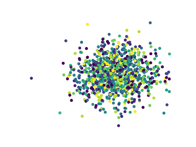
(a) Epoch 0

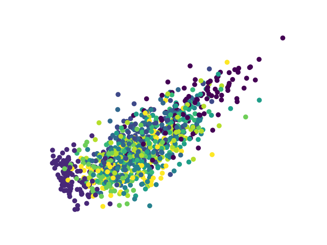
(b) Epoch 100

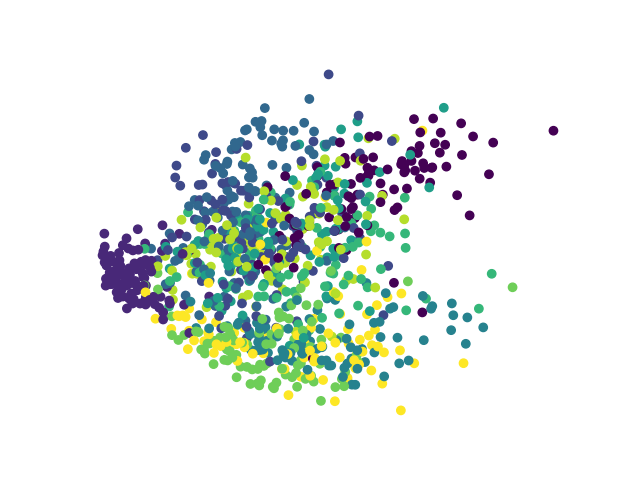
(c) Epoch 500 (final)

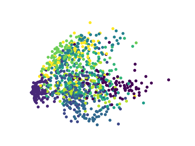
(d) Standard PCA

Figure 2: PCA on 1000 MNIST samples by gradient descent. The final result is equivalent to the standard PCA embedding up to orthogonal transformation.

5 AR Problems with Two Kernels

Using the blueprint developed in sections 3 and 4, we now show that ARDR methods such as UMAP can be emulated using classical methods and gradient descent. The key observation is simply that ARDR methods have a kernel on $\mathbf{Y}$ while classical methods do not. Unfortunately, this kernel is also what introduces much of the difficulty when analyzing convergence properties.

To see this, consider that the above theoretical results on PCA hold for the linear kernel on $\mathbf{Y}$ but no longer hold as soon as $k_{y}$ is non-linear. This is due to the fact that differentiating with respect to $k_{y}$ induces a new scalar by the chain rule. Indeed, the AR problem $\mathcal{L}_{\mathcal{F}}(\mathbf{X},\mathbf{Y})$ will necessarily have gradients acting on $y_{i}$ of the form

$$\nabla_{y_{i}}=\sum_{j}l_{ij}\cdot\dfrac{d\;k_{y}(||y_{i}-y_{j}||_{2}^{2})}{d\;||y_{i}-y_{j}||_{2}^{2}}\cdot(y_{i}-y_{j}),$$ (5)

where $l_{ij}$ depends on $k_{x}$, $k_{y}$, and the chosen loss function $\mathcal{F}$. We derive Equation 5 in the proof of Lemma 4. Observe that if $k_{y}$ is the centered linear kernel then the derivative term is constant. Note, if $\mathcal{F}$ is the Frobenius norm, then $l_{ij}=[\mathbf{K}_{X}-\mathbf{K}_{Y}]_{ij}$.

We relied on these observations heavily when proving the results in Section 4. Specifically, for $\mathbf{K}_{Y}\!\!\sim\!\!\mathbf{G}_{Y}$, the optimal solution must have $\mathbf{K}_{X}-\mathbf{K}_{Y}$ of rank $D-d$ while $\mathbf{Y}$ has rank $d$. Thus, $(\mathbf{K}_{X}-\mathbf{K}_{Y})\mathbf{Y}$ must be zero by orthogonality. However, a non-linear $k_{y}$ impedes this line of reasoning. First, it is unclear what dynamics the non-constant derivative term in Eq. 5 introduces. Second, the above orthogonality argument is broken for non-linear $k_{y}$ – we could have that $\text{rank}(\mathbf{K}_{Y})>d$ even when $\text{rank}(\mathbf{Y})=d$. Nonetheless, we will now verify that a non-linear $k_{y}$ introduces attraction-repulsion characteristics like those in ARDR methods.

5.1 PCA with Two Kernels

Recall the PCA objective function $\mathcal{L}_{PCA}(\mathbf{X},\mathbf{Y})=||\mathbf{C}(\mathbf{G}_{X}-\mathbf{G}_{Y})\mathbf{C}||_{F}^{2}$. We now replace the centered Gram matrices $\mathbf{C}\mathbf{G}_{X}\mathbf{C}$ and $\mathbf{C}\mathbf{G}_{Y}\mathbf{C}$ by their kernel counterparts $\mathbf{K}_{X}$ and $\mathbf{K}_{Y}$. Our loss function is then $\mathcal{L}_{PCA}^{2-Kernel}(\mathbf{X},\mathbf{Y})=||\mathbf{K}_{X}-\mathbf{K}_{Y}||_{F}^{2}$, leading to a gradient of the form

$$\nabla_{y_{i}}=-\sum_{j}(k_{x}(x_{i},x_{j})-k_{y}(y_{i},y_{j}))\cdot\dfrac{d\;k_{y}(||y_{i}-y_{j}||_{2}^{2})}{d\;||y_{i}-y_{j}||_{2}^{2}}\cdot(y_{i}-y_{j})$$ (6)

It was shown in [52] that applying these gradients with the UMAP optimization scheme provides embeddings that are indistinguishable from the standard UMAP embeddings. However, we show in Figure 3 that this does not hold when optimizing all $O(n^{2})$ pairwise forces. This is in line with the observations made in [48] regarding what loss UMAP is actually optimizing – applying some of the gradients in Eq. 6 gives embeddings indistinguishable from UMAP but optimizing all $n^{2}$ pairs of points does not. Thus, reproducing ARDR embeddings in terms of classical techniques requires a method that prioritizes local/global relationships similarly to tSNE and UMAP.

5.2 LLE with Two Kernels

LLE is therefore a natural choice as it finds the $\mathbf{Y}$ that preserves the local relationships in $\mathbf{X}$. We now verify this by presenting gradients that optimize the LLE objective under two kernels.

For simplicity’s sake, we will assume that the constraint $\frac{1}{n}\mathbf{Y}^{\top}\mathbf{Y}=\mathbf{I}$ applies in kernel space. The closest suitable constraint is then $\frac{1}{n}\mathbf{K}_{Y}=\mathbf{I}$, as this implies that $\psi(\mathbf{Y})$ is an orthogonal basis and will also have covariance matrix $\mathbf{I}$. Notice that the diagonal of both $\mathbf{K}_{Y}$ and $\mathbf{I}$ is always 1, implying that the constraint requires the off-diagonals of $\mathbf{K}_{Y}$ to be 0. Thus, we will approximate the solution to LLE with two kernels by minimizing the loss $\mathcal{L}_{LLE}(\mathbf{W},\mathbf{Y})=\text{Tr}(\mathbf{M}\mathbf{K}_{Y})+\frac{1}{n}\sum_{i,j}k_{y}(||y_{i}-y_{j}||)_{2}^{2}$, for $\mathbf{M}=(\mathbf{I}-\mathbf{W})^{\top}(\mathbf{I}-\mathbf{W})$.

Given this loss function, assume that we have the $\mathbf{W}$ that represents nearest neighborhoods in $\mathbf{X}$. We now want to use gradient descent to find the $\mathbf{Y}$ such that $\mathcal{L}_{LLE}(\mathbf{W},\mathbf{Y})$ is minimized. Our next lemma shows that this has a very natural interpretation in the A/R framework.

Lemma 4.

Let $\mathbf{Y}$ and $\mathbf{M}$ be defined as above, let $\mathbf{V}=\mathbf{W}^{\top}\mathbf{W}$, and let $c$ be a constant. Then the gradient of $\text{Tr}\left(\mathbf{M}\mathbf{K}_{Y}\right)+\frac{1}{n}\sum_{i,j}k_{y}(||y_{i}-y_{j}||)_{2}^{2}$ with respect to $y_{i}$ is given by

$$\nabla_{y_{i}}=c\sum_{j}\left(w_{ij}+w_{ji}-v_{ij}-\frac{1}{n}\right)\dfrac{d\;k_{y}(||y_{i}-y_{j}||_{2}^{2})}{d\;||y_{i}-y_{j}||_{2}^{2}}(y_{i}-y_{j}).$$

The proof can be found in Section B.2 of the supplementary material.

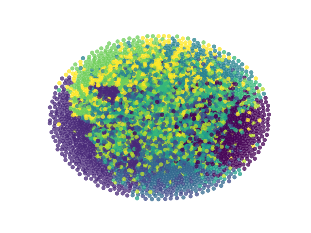
(a) PCA with $k_{x},k_{y}$

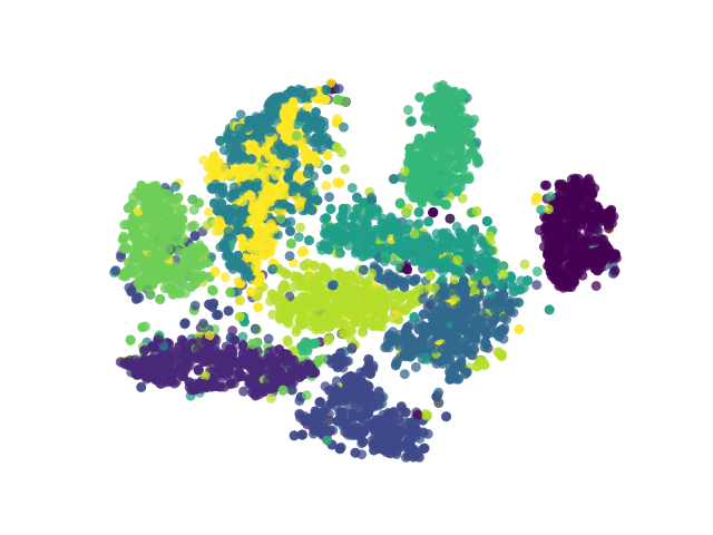
(b) tSNE

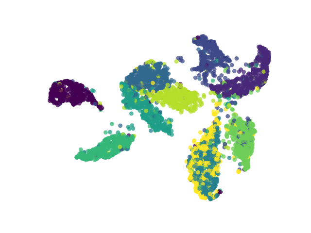
(c) UMAP

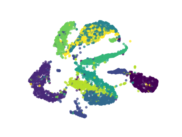
(d) LLE with $k_{x},k_{y}$

Figure 3: Left: Embedding by grad. descent of the PCA objective function with the UMAP $k_{x}$ and $k_{y}$ functions. Middle: tSNE and UMAP embeddings. Right: Embedding by grad. descent of the LLE objective function with the UMAP $k_{x}$ and $k_{y}$ functions. The dataset is 5K randomly chosen points from the MNIST dataset. We observe similar separation of the classes in LLE with two kernels vs. tSNE and UMAP.

We take a moment to consider the striking similarities between this and UMAP’s gradients. First, note that for $k_{y}\sim(1-||y_{i}-y_{j}||_{2}^{2})^{-1}$ as in UMAP, the derivative with respect to the distance incurs a minus sign. Given this, the terms $w_{ij}$ and $w_{ji}$ constitute our attraction scalars, i.e. the attraction between $y_{i}$ and $y_{j}$ depends linearly on how much $x_{j}$ (resp. $x_{i}$) contributes to $x_{i}$’s (resp. $x_{j}$’s) local neighborhood under $k_{x}$. Indeed, this is precisely what the UMAP attraction scalars constitute. Furthermore, in UMAP’s implementation, when $y_{i}$ is attracted to $y_{j}$, $y_{j}$ is also attracted to $y_{i}$ [52].

Now consider the repulsive terms in Lemma 4 given by $v_{ij}+1/n=\left[\mathbf{W}^{\top}\mathbf{W}\right]_{ij}+1/n$. Since $\mathbf{W}$ is an adjacency matrix with $k$ entries in each row, the first term is equal to the sum of the weights over all paths of length 2 from $x_{i}$ to $x_{j}$. That is, $v_{ij}$ imposes repels $y_{i}$ from $y_{j}$ based on how densely connected $x_{i}$ and $x_{j}$ are. The second repulsion scalar $1/n$ is simply an average repulsion from all points in $\mathbf{Y}$. Now recall that UMAP’s repulsion heuristic samples a constant number of points from $\mathbf{Y}$ for each $y_{i}$. For distant points, these repulsions are effectively 0, implying that UMAP’s practical repulsions are, in expectation, somewhere between the $v_{ij}$ and $1/n$ terms from Lemma 4.

We visualize this in similarity Figure 3, where we show the tSNE, UMAP and 2-kernel PCA and LLE embeddings on 5K points from the MNIST training set. For the 2-kernel implementations, we simply calculate the loss function the corresponding loss function in Pytorch and run standard gradient descent on it. Importantly, we use none of the heuristics that are present in the tSNE and UMAP algorithms [66, 2, 52]. The message is that the most vanilla implementation of LLE with UMAP’s kernels adequately reproduces ARDR embeddings.

6 Future Work

Before discussing our conjectures and future work, we mention that they are directed at our primary open question: “What information does an optimal ARDR-like embedding give regarding its input?” In order to answer this, one must have a definition of what it means to find an ‘optimal ARDR-like’ embedding. To that end, we point out that there seems to be a fundamental divide between the modern and classical DR methods and that quantifying how ‘similar’ two algorithms’ embeddings are is a difficult task [52, 53]. Thus, in the absence of consensus on a metric that can do this, we will discuss our conjectures using the theoretical metric $f^{*}$ that optimally differentiates between classical and modern DR methods. Although it is infeasible to find such a metric in practice, identifying a measure that adequately approximates $f^{*}$ should serve to make our conjectures falsifiable. We note that finding a metric that resembles $f^{*}$ is a major open question and has been discussed in [53, 77, 69, 49].

6.1 Towards an Optimal Metric

Let $\mathbf{Y}_{1}$ and $\mathbf{Y}_{2}$ be two embeddings obtained from algorithms $\mathcal{A}_{1}$ and $\mathcal{A}_{2}$ on the same input, i.e. $\mathcal{A}_{1}(\mathbf{X})=\mathbf{Y}_{1}$ and $\mathcal{A}_{2}(\mathbf{X})=\mathbf{Y}_{2}$. We now define the space of metrics $\mathcal{M}$ that accept $\mathbf{Y}_{1}$ and $\mathbf{Y}_{2}$ and output a value in $[0,1]$. We now consider the optimal metric $f^{*}\in\mathcal{M}$ as the one that maximally differentiates between classical DR methods (PCA, LLE, ISOMAP, LE, MDS, etc.) and the modern ones (tSNE, UMAP, etc). That is, in expectation over the set of all inputs $\mathcal{X}$, $f^{*}$ gives maximal scores when the embeddings come from the same class of DR methods and minimal scores when they come from different classes of methods. In some sense, $f^{*}$ is a measure for the fundamental difference in embeddings between modern and classical DR methods. Equipped with this definition, we now proceed to our conjectures regarding the essence underlying tSNE and UMAP.

6.2 Conjectures

In Section 5, we showed that pairing the classical DR methods with a kernel on $\mathbf{Y}$ gives gradients that have a very similar form to those in ARDR methods. Furthermore, we verified that minimizing the objective of LLE with UMAP’s $k_{x},k_{y}$-kernels gives similar embeddings as UMAP and tSNE. This implies that the primary difference between the classical and ARDR methods is the kernel on $\mathbf{Y}$. Specifically, let $f^{*}$ be as defined in Section 6.1. Then,

Conjecture 1.

Let $\mathbb{E}_{x\in\mathcal{X}}\left[\nabla^{umap}_{y_{i}}\right]$ be the expected gradient calculated during an epoch of UMAP for a given embedding $\mathbf{Y}$. Let $\nabla^{lle}_{y_{i}}$ be defined as in Lemma 4. Then $\mathbb{E}_{x\in\mathcal{X}}\left[\langle\nabla^{umap},\nabla^{lle}\rangle_{F}\right]>0$, where $\langle\cdot,\cdot\rangle_{F}$ denotes the Frobenius inner product. Furthermore, embeddings found by gradient descent on LLE with the UMAP kernels will, under $f^{*}$, have high similarity to embeddings found by UMAP and low similarity to those found by classical methods.

That is, we claim that a gradient step for LLE with the UMAP kernels is, on average, going to act on the embedding similarly to UMAP and that the final embeddings will have similar structure under $f^{*}$. This is a formalization of the statement ‘UMAP approximates LLE with two kernels’.

Although the above conjecture describes how one could frame UMAP in terms of the classical algorithms, it states nothing about convergence guarantees. Indeed, we have seen that performing PCA in the ARDR framework with gradient descent converges to the true PCA embedding. It remains to be seen if this holds in the presence of non-linear $k_{y}$ kernels. However, if Conjecture 1 is true, then we believe that there should exist a direct method similar to LLE that emulates tSNE/UMAP:

Conjecture 2.

Let $\mathcal{A}$ be an ARDR algorithm that has high similarity to UMAP and low similarity to classical methods under $f^{*}$ and let $\mathcal{L}$ be $\mathcal{A}$’s effective loss function. Let $OPT_{x}$ be the embedding with minimal cost for $\mathcal{A}$ on $x\in\mathcal{X}$ under $\mathcal{L}$. Then there exists an algorithm $\mathcal{A}^{\prime}$ that returns $\mathcal{A}^{\prime}(x)=\mathbf{Y}_{x}^{\prime}$ without iterative optimizations such that $\mathcal{L}(\mathbf{Y}_{x}^{\prime})\in(1\pm\varepsilon)\mathcal{L}(OPT_{x})$ for all $x\in\mathcal{X}$.

By effective loss function, we mean the loss that is being optimized by the specific heuristics and implementation of $\mathcal{A}$; we refer to [48] for an example regarding UMAP. This conjecture is a formalization of the statement ‘an algorithm similar to UMAP can be performed without gradient descent and can provably approximate the global minimum of UMAP’.

If we assume the above conjectures are true, we now propose that we can transfer the explainability of PCA and LLE to the ARDR setting. That is, if one can get the same quality embedding by solving for it directly, then one would understand how well the embedding actually preserves the structure of the dataset. In a formal sense, we believe that the major open question surrounding tSNE and UMAP is the following:

Question 1.

Let $\mathcal{A}$ be an ARDR algorithm that is similar to tSNE/UMAP under $f^{*}$ and let $OPT_{\mathcal{A}}(x)$ be the optimal embedding under $\mathcal{A}$ for input $x$. Now consider all $\{x_{1},x_{2},...,x_{n}\}\in\mathcal{X}$ such that $OPT_{\mathcal{A}}(x_{1})=OPT_{\mathcal{A}}(x_{2})=...=OPT_{\mathcal{A}}(x_{n})$. Then what characteristics must be consistent across all $x\in\{x_{1},...,x_{n}\}$?

This is perhaps the most fundamental explainability question that one can ask: “given the output of the explainability method, what can one say about the input?”

We note that our conjectures directly help to answer this question. First, our discussion on metrics describes what characteristics a ‘similar’ algorithm to tSNE/UMAP must exhibit. Second, we believe that LLE with two kernels is precisely the ARDR algorithm that is ‘similar’ to tSNE/UMAP. Lastly, we conjecture that such an ARDR algorithm can be solved directly, i.e. without relying on attractions and repulsions. This would allow one to formally state which inputs map to the same embedding and, inevitably, what qualities must be consistent across all of these inputs.

Appendix A PCA theoretical results

A.1 Proof of Theorem 1

Proof.

The proof relies on a change of basis in the first $d$ components of $\mathbf{C}\mathbf{X}$ and $\mathbf{C}\mathbf{Y}$. Let $\mathbf{C}\mathbf{X}=\mathbf{U}_{X}\mathbf{\Sigma}_{X}\mathbf{V}_{X}^{\top}$ and $\mathbf{C}\mathbf{Y}=\mathbf{U}_{Y}\mathbf{\Sigma}_{Y}\mathbf{V}_{Y}^{\top}$ be the SVD of $\mathbf{C}\mathbf{X}$ and $\mathbf{C}\mathbf{Y}$. Then $\mathbf{C}\mathbf{G}_{X}\mathbf{C}=\mathbf{U}_{X}\mathbf{\Sigma}_{X}^{2}\mathbf{U}_{X}^{\top}$ and $\mathbf{C}\mathbf{G}_{Y}\mathbf{C}=\mathbf{U}_{Y}\mathbf{\Sigma}_{Y}^{2}\mathbf{U}_{Y}^{\top}$.

We now decompose $\mathbf{C}\mathbf{X}=\mathbf{U}_{X}^{+}\mathbf{\Sigma}_{X}^{+}(\mathbf{V}_{X}^{+})^{\top}+\mathbf{U}_{X}^{-}\mathbf{\Sigma}_{X}^{-}(\mathbf{V}_{X}^{-})^{\top}$, where the $+$ superscript corresponds to the first $d$ components of $\mathbf{C}\mathbf{X}$ and the $-$ superscript corresponds to the final $D-d$ components. Note that now $\mathbf{U}_{X}^{+}$ is an orthogonal transformation in the same subspace as $\mathbf{U}_{Y}$. This allows us to define $\mathbf{O}=\mathbf{U}_{Y}(\mathbf{U}_{X}^{+})^{\top}$ as the change of basis from $\mathbf{C}\mathbf{G}_{X}\mathbf{C}$ to $\mathbf{C}\mathbf{G}_{Y}\mathbf{C}$, providing the following characterization of $L_{PCA}(\mathbf{X},\mathbf{Y})$:

$$L_{PCA}(\mathbf{X},\mathbf{Y};\mathbf{O})=||\mathbf{O}\mathbf{C}\mathbf{G}_{X}\mathbf{C}\mathbf{O}^{\top}-\mathbf{C}\mathbf{G}_{Y}\mathbf{C}||_{F}^{2}=||(\mathbf{U}_{Y}((\mathbf{\Sigma}_{X}^{+})^{2}-\mathbf{\Sigma}_{Y}^{2})\mathbf{U}_{Y}^{\top})+f(\mathbf{X})||_{F}^{2}$$ (8)

where $f(\mathbf{X})$ is independent of $\mathbf{Y}$. The minimum of Equation 8 over $\mathbf{Y}$ occurs when $\mathbf{C}\mathbf{Y}$ has the same singular values as $\mathbf{O}\mathbf{C}\mathbf{X}$ in the first $d$ components, which is exactly the PCA projection of $\mathbf{X}$ up to orthonormal transformation.

It remains to show that PCA is invariant to orthonormal transformations. Let $\mathbf{X}^{\prime}=\mathbf{O}\mathbf{X}$. Then $\mathbf{G}_{X}^{\prime}=\mathbf{X}^{\prime}(\mathbf{X}^{\prime})^{\top}=\mathbf{O}\mathbf{G}_{X}\mathbf{O}^{\top}=\mathbf{G}_{X}$, since Gram matrices are unique up to orthogonal transformations. ∎

A.2 PCA gradient derivation

Let $\mathbf{Y}$ be any set of points in $\mathbb{R}^{n\times d}$. Then the gradient with respect to $\mathbf{Y}$ of $\mathcal{L}_{PCA}(\mathbf{X},\mathbf{Y})=||\mathbf{C}\mathbf{G}_{X}\mathbf{C}-\mathbf{C}\mathbf{G}_{Y}\mathbf{C}||_{F}^{2}$ is obtained by

$$d\;\mathcal{L}_{PCA}(\mathbf{X},\mathbf{Y}) =d\;||\mathbf{C}(\mathbf{G}_{X}-\mathbf{G}_{Y})\mathbf{C}||_{F}^{2}$$

$$=d\;\left(\left(\mathbf{C}(\mathbf{G}_{X}-\mathbf{G}_{Y})\mathbf{C}\right)^{\top}:\left(\mathbf{C}(\mathbf{G}_{X}-\mathbf{G}_{Y})\mathbf{C}\right)\right)$$

$$=2(\mathbf{C}(\mathbf{G}_{X}-\mathbf{G}_{Y})\mathbf{C})^{\top}:d(\mathbf{C}(\mathbf{G}_{X}-\mathbf{G}_{Y})\mathbf{C})$$

$$=-2\mathbf{C}(\mathbf{G}_{X}-\mathbf{G}_{Y})\mathbf{C}:d\mathbf{G}_{Y}$$

$$=-4\mathbf{C}(\mathbf{G}_{X}-\mathbf{G}_{Y})\mathbf{C}\mathbf{Y}:d\mathbf{Y}$$

$$\frac{d\;f_{PCA}(\mathbf{X},\mathbf{Y})}{d\mathbf{Y}} =-4\mathbf{C}(\mathbf{G}_{X}-\mathbf{G}_{Y})\mathbf{C}\mathbf{Y}$$

where $:$ represents the Frobenius inner product and the centering matrices cancel due to idempotence.

A.3 Proof of Lemma 2

Proof.

We use the well-known fact that $\mathbf{C}\mathbf{G}_{Y}\mathbf{C}=-\frac{1}{2}\mathbf{C}\mathbf{D}_{Y}\mathbf{C}$, for squared Euclidean distance matrix $\mathbf{D}_{Y}$, to express the gradient in terms of $(y_{i}-y_{j})$ vectors.

$$\nabla =\alpha\mathbf{L}:d\left(-\frac{1}{2}\mathbf{C}\mathbf{D}_{Y}\mathbf{C}\right)$$

$$=-\frac{\alpha}{2}\mathbf{L}:d\mathbf{D}_{Y}\quad (\text{$\mathbf{C}$ cancels by idempotence})$$

$$\implies\nabla_{y_{i}} =-\alpha\sum_{j}[\mathbf{L}]_{ij}(y_{i}-y_{j})$$

∎

A.4 Proof of Theorem 1

We start by confirming that the PCA embedding is a minimum of the gradient. Recall that our gradient is of the form

$$\nabla_{\mathbf{Y}}=4\mathbf{C}(\mathbf{G}_{X}-\mathbf{G}_{Y})\mathbf{C}\mathbf{Y}.$$

If $\mathbf{C}\mathbf{Y}$ is the PCA embedding of $\mathbf{C}\mathbf{X}$, then $\mathbf{C}\mathbf{Y}$’s $d$ singular values should be $\mathbf{C}\mathbf{X}$’s top-$d$ singular values. Given this, $\mathbf{C}(\mathbf{G}_{X}-\mathbf{G}_{Y})\mathbf{C}$ will only have singular values corresponding to the remaining $D-d$ diagonal positions. However, notice that $\mathbf{Y}$’s singular values are still in the first $d$ coordinates. Since $\mathbf{G}_{X}$ and $\mathbf{G}_{Y}$ have the same orthonormal basis, we see that $\mathbf{C}(\mathbf{G}_{X}-\mathbf{G}_{Y})\mathbf{C}$ is orthogonal to $\mathbf{Y}$, giving us 0 gradient when $\mathbf{Y}$ is the PCA embedding.

Next, we show that any minimum of the objective function must be a global minimum. This is a simple extension of the proof of lemma 1. Assume for the sake of contradiction that $\mathbf{Z}$ is a global minimum of $\mathcal{L}_{PCA}$ that is not equal to the PCA embedding. Then $\mathbf{Z}\neq\mathbf{O}\mathbf{Y}$ for some orthonormal transformation $\mathbf{O}$, implying that the singular values of $\mathbf{Z}$ do not equal those of $\mathbf{X}$ in the first $d$ components. Thus, there is a $\mathbf{Z}^{\prime}$ in the $\varepsilon$-ball of $\mathbf{Z}$ that better approximates the singular values of $\mathbf{X}$. Thus, $\mathbf{Z}$ cannot be a minimum.

Given this, we now want to show that there always exists a learning rate value such that a step of gradient descent will decrease our cost. Let $\mathbf{Y}^{\prime}=(\mathbf{I}+\gamma\mathbf{L})\mathbf{Y}$ be the embedding after one step of gradient descent with learning rate $\gamma$ and $\mathbf{L}=\mathbf{C}(\mathbf{G}_{X}-\mathbf{G}_{Y})\mathbf{C}$.

$$\mathcal{L}_{PCA}(\mathbf{X},\mathbf{Y}^{\prime})<\mathcal{L}_{PCA}(\mathbf{X},\mathbf{Y}) \rightarrow||\mathbf{C}(\mathbf{G}_{X}-\mathbf{Y}^{\prime}\mathbf{Y}^{\prime\top})\mathbf{C}||_{F}^{2}<||\mathbf{C}(\mathbf{G}_{X}-\mathbf{G}_{Y})\mathbf{C}||_{F}^{2}$$

$$||\mathbf{C}(\mathbf{X}\mathbf{X}^{\top}-\mathbf{Y}^{\prime}\mathbf{Y}^{\prime\top})\mathbf{C}||_{F}^{2} =||\mathbf{C}\left(\mathbf{G}_{X}-\left((I+\gamma\mathbf{L})\mathbf{Y}\right)\left((I+\gamma\mathbf{L})\mathbf{Y}\right)^{\top}\right)\mathbf{C}||_{F}^{2}$$

$$=||\mathbf{C}(\mathbf{G}_{X}-\mathbf{G}_{Y})\mathbf{C}-\gamma\mathbf{C}\left(\mathbf{L}\mathbf{G}_{Y}-\mathbf{G}_{Y}\mathbf{L}^{\top}-\gamma\mathbf{L}\mathbf{G}_{Y}\mathbf{L}^{\top}\right)\mathbf{C}||_{F}^{2}$$

This expression subtracts $\gamma\mathbf{C}\left(\mathbf{L}\mathbf{G}_{Y}+\mathbf{G}_{Y}\mathbf{L}^{\top}+\gamma\mathbf{L}\mathbf{G}_{Y}\mathbf{L}^{\top}\right)\mathbf{C}$ from our initial matrix $\mathbf{C}(\mathbf{G}_{X}-\mathbf{G}_{Y})\mathbf{C}$. Thus, the overall Frobenius norm of the difference will be smaller than that of $\mathbf{C}(\mathbf{G}_{X}-\mathbf{G}_{Y})\mathbf{C}$ if the two matrices point in the same direction. Said otherwise, we want to find a $\gamma$ such that

$$0<\langle\mathbf{C}\left(\mathbf{L}\mathbf{G}_{Y}+\mathbf{G}_{Y}\mathbf{L}^{\top}+\gamma\mathbf{L}\mathbf{G}_{Y}\mathbf{L}^{\top}\right)\mathbf{C},\mathbf{C}(\mathbf{G}_{X}-\mathbf{G}_{Y})\mathbf{C}\rangle_{F}$$

Applying the properties of the trace as the Frobenius inner product, we get

$$\text{Tr}\left[\left(\mathbf{C}(\mathbf{L}\mathbf{G}_{Y}+\mathbf{G}_{Y}\mathbf{L}^{\top}+\gamma\mathbf{L}\mathbf{G}_{Y}\mathbf{L}^{\top})\mathbf{C}\right)^{\top}\mathbf{C}(\mathbf{G}_{X}-\mathbf{G}_{Y})\mathbf{C}\right]=$$

$$=\text{Tr}\left[\left(\mathbf{C}(\mathbf{L}\mathbf{G}_{Y}+\mathbf{G}_{Y}\mathbf{L}^{\top}+\gamma\mathbf{L}\mathbf{G}_{Y}\mathbf{L}^{\top})\mathbf{C}\right)^{\top}\mathbf{L}\right]$$

$$=\text{Tr}\left[2\mathbf{L}^{2}\mathbf{G}_{Y}\mathbf{L}+\gamma\mathbf{L}^{2}\mathbf{G}_{Y}\mathbf{L}\right]$$

$$=\text{Tr}\left[2\mathbf{L}^{2}\mathbf{G}_{Y}+\gamma\mathbf{L}^{3}\mathbf{G}_{Y}\right]$$

$$=\text{Tr}\left[2(\mathbf{C}(\mathbf{G}_{X}-\mathbf{G}_{Y})\mathbf{C})^{2}\mathbf{G}_{Y}\right]+\gamma\text{Tr}\left[(\mathbf{C}(\mathbf{G}_{X}-\mathbf{G}_{Y})\mathbf{C})^{3}\mathbf{G}_{Y}\right]$$ (9)

where we cancelled the $\mathbf{C}$ matrices by idempotence with respect to the $\mathbf{C}$’s in $\mathbf{L}$.

Now notice that the first term is necessarily non-negative as it is the trace of a positive semidefinite matrix. Furthermore, it will only be zero if $\mathbf{G}_{X}=\mathbf{G}_{Y}$ or $\mathbf{G}_{Y}=0$. In both of these cases our gradient descent has completed, so we can assume the first term to be strictly positive.

If $\mathbf{G}_{Y}\preceq\mathbf{G}_{X}$, then the second is also positive semidefinite and non-negative. This is intuitively clear, as $\mathbf{G}_{Y}\preceq\mathbf{G}_{X}$ implies that our problem is entirely convex. Indeed, this means that as long as our learning rate isn’t so large that it ‘overshoots’ the convex subspace, we are guaranteed to minimize our loss when $\mathbf{G}_{Y}\preceq\mathbf{G}_{X}$. In the alternative setting where $\mathbf{G}_{Y}\precneq\mathbf{G}_{X}$, we simply need to choose a small enough $\gamma$ such that expression A.4 remains positive. This concludes the proof.

A.5 Proof of Lemma 3

The proof relies on defining $\mathbf{G}_{X}^{\prime}=\mathbf{G}_{X}+\mathbf{R}_{X}$ and $\mathbf{G}_{Y}^{\prime}=\mathbf{G}_{Y}+\mathbf{R}_{Y}$ as the sum of the original Gram matrices plus residual matrices $\mathbf{R}$. Then

$$||\mathbf{R}_{X}||_{F}^{2}=(1+\epsilon)||\mathbf{G}_{X}-\mathbf{G}_{X}^{k}||_{F}^{2}=(1+\epsilon)\sum_{i=k+1}^{n}\sigma_{xi}^{2}$$

where $\sigma_{xi}$ is the i-th singular value of $\mathbf{G}_{X}$. Notice that since $\mathbf{G}_{Y}^{K}=\mathbf{G}_{Y}$ for $k\leq d$, we have $\mathbf{R}_{Y}=0$.

Plugging these in, we get

$$\langle\nabla,\nabla^{\prime}\rangle_{F} =\text{Tr}\left[C(G_{X}-G_{Y})CYY^{T}C(G^{\prime}_{X}-G^{\prime}_{Y})C\right]$$

$$=\text{Tr}\left[C(G_{X}-G_{Y})CG_{Y}C\left[(G_{X}-G_{Y})-(R_{X}-R_{Y})\right]C\right]$$

$$=\text{Tr}\left[(G_{X}-G_{Y})CG_{Y}C\left[(G_{X}-G_{Y})-R_{X}\right]C\right]$$

$$=\text{Tr}\left[\left((G_{X}-G_{Y})CG_{Y}C(G_{X}-G_{Y})\right)-\left((G_{X}-G_{Y})CG_{Y}CR_{X}\right)C\right]$$

$$=\text{Tr}\left[(G_{X}-G_{Y})^{2}CG_{Y}C\right]-\text{Tr}\left[C(G_{X}-G_{Y})CG_{Y}CR_{X}\right]$$

where we perform rearrangements and cancel one of the $C$’s due to the trace being invariant to cyclic permutations.

Notice that the first term $\text{Tr}\left((G_{X}-G_{Y})^{2}CG_{Y}C\right)$ must be positive as it is the trace of a positive semi-definite matrix. It then suffices to show that

$$\text{Tr}\left((G_{X}-G_{Y})^{2}CG_{Y}C\right)>|\text{Tr}\left(C(G_{X}-G_{Y})CG_{Y}CR_{X}\right)|$$

If this condition is satisfied, then we have that $\langle\nabla,\nabla^{\prime}\rangle_{F}>0$, allowing us to employ subgradient descent methods.

$$\langle\nabla,\nabla^{\prime}\rangle \geq\text{Tr}\left((G_{X}-G_{Y})^{2}CG_{Y}C\right)-|\text{Tr}\left(C(G_{X}-G_{Y})G_{Y}R_{X}\right)|$$

$$\geq\text{Tr}\left((G_{X}-G_{Y})^{2}CG_{Y}C\right)-c\cdot||(G_{X}-G_{Y})(CG_{Y}C)^{1/2}||_{F}\cdot||(CG_{Y}C)^{1/2}R_{X}||_{F}$$

$$=||(G_{X}-G_{Y})(CG_{Y}C)^{1/2}||_{F}^{2}-c||(G_{X}-G_{Y})(CG_{Y}C)^{1/2}||_{F}\cdot||(CG_{Y}C)^{1/2}R_{X}||_{F}$$

$$=||(G_{X}-G_{Y})(CG_{Y}C)^{1/2}||_{F}\left(||(CG_{Y}C)^{1/2}(G_{X}-G_{Y})||_{F}-c\cdot||(CG_{Y}C)^{1/2}R_{X}||_{F}\right)$$

where $c=||C||_{F}^{2}$.

Since the first term $||(G_{X}-G_{Y})(CG_{Y}C)^{1/2}||_{F}$ is necessarily positive, we have that $\langle\nabla,\nabla^{\prime}\rangle_{F}\geq 0$ as long as $||(CG_{Y}C)^{1/2}(G_{X}-G_{Y})||_{F}-c\cdot||(CG_{Y}C)^{1/2}R_{X}||_{F}\geq 0$ We can also remove the $c$ scalar, since we know that $c>1$. This gives us the necessary condition

$$||(CG_{Y}C)^{1/2}(G_{X}-G_{Y})||_{F}-||(CG_{Y}C)^{1/2}R_{X}||_{F}\geq 0\implies\langle\nabla,\nabla^{\prime}\rangle_{F}\geq 0$$ (10)

We can think of $(CG_{Y}C)^{1/2}$ as any dataset with the same principal components as $CY$. So this necessary condition is effectively saying that the inner product between $CY$ and $(G_{X}-G_{Y})$ must be bigger than the inner product between $CY$ and $R_{X}$. This intuitively makes sense. Consider that $G_{X}-G_{Y}$ is the amount of error in our current projection $CY$. Meanwhile, $R_{X}$ is an $\epsilon$-approximation of $G_{X}^{k}$, the optimal low-rank representation of $G_{X}$. So our necessary condition states that as long as $G_{Y}$ is not an $\epsilon$-approximation of $G_{X}$, we can continue to use the sublinear-time approximation of $G_{X}$ to approximate the gradient $\nabla$.

Said otherwise, if $G_{Y}$ is sufficiently different from $G_{X}$, then $\langle\nabla,\nabla^{\prime}\rangle_{F}$ is positive. If not, then we have that $G_{Y}$ is approximates $G_{X}^{k}$, the optimal low-rank approximation of $G_{X}$. We formalize this below.

Let $G_{Y}$ be such that $||G_{X}-G_{Y}||_{F}^{2}\geq(1+\alpha)||G_{X}-G_{X}^{k}||_{F}^{2}$ for $\alpha>0$. Then we want to solve for the $\alpha$ that makes equation 10 necessarily positive. This is equivalent to finding the $\alpha$ that satisfies $\min||(G_{X}-G_{Y})(CG_{Y}C)^{1/2}||_{F}=\max||(CG_{X}C)^{1/2}R_{X}||_{F}$. We then obtan a lower bound for the minimum:

$$||(G_{X}-G_{Y})(CG_{Y}C)^{1/2}||_{F} \geq\sigma_{min}\left((CG_{Y}C)^{1/2}\right)\cdot||G_{X}-G_{Y}||_{F}$$

$$\geq\sigma_{min}\left((CG_{Y}C)^{1/2}\right)\cdot\sqrt{(1+\alpha)||G_{X}-G_{X}^{k}||_{F}^{2}}$$

and an upper bound for the maximum:

$$||(CG_{Y}C)^{1/2}R_{X}||_{F} \leq||(CG_{Y}C)^{1/2}||_{2}||R_{X}||_{F}$$

$$\leq||(CG_{Y}C)^{1/2}||_{2}\cdot\sqrt{(1+\epsilon)||G_{X}-G_{X}^{k}||_{F}^{2}}$$

$$\leq\sigma_{max}\left((CG_{Y}C)^{1/2}\right)\cdot\sqrt{(1+\epsilon)||G_{X}-G_{X}^{k}||_{F}^{2}}$$

Setting the lower bound equal to the upper bound and solving for $\alpha$ tells us that equation 10 is greater than 0 when $\alpha$ satisfies

$$\alpha >\dfrac{\lambda_{y_{1}}}{\lambda_{y_{k}}}\cdot\dfrac{(1+\epsilon)||G_{X}-G_{X}^{k}||_{2}^{2}}{||G_{X}-G_{X}^{k}||_{F}^{2}}-1$$

$$=(1+\epsilon)\dfrac{\lambda_{y_{1}}}{\lambda_{y_{k}}}-1$$

This means that our gradient $\nabla^{\prime}$ will be in line with the true gradient $\nabla$ as long as $G_{Y}$ satisfies the following condition:

$$||G_{X}-G_{Y}||_{F}^{2}\geq(1+\epsilon)\dfrac{\lambda_{y_{1}}}{\lambda_{y_{k}}}||G_{X}-G_{X}^{k}||_{F}^{2}$$

As long as this is true, the gradient will push $Y$ into the direction of the PCA embedding of $X$ in $k$ dimensions. If we initialize our $Y$ such that $\lambda_{y_{1}}\approx\lambda_{y_{k}}$, then we know they will slowly diverge over the course of gradient descent. Thus, we can upper bound the ratio $\lambda_{y_{1}}/\lambda_{y_{k}}\leq\lambda_{x_{1}}/\lambda_{x_{k}}$. This gives us our final condition for convergence:

$$\langle\nabla,\nabla^{\prime}\rangle_{F}\text{ will be greater than 0 as long as }||G_{X}-G_{Y}||_{F}^{2}\geq(1+\epsilon)\dfrac{\lambda_{x_{1}}}{\lambda_{x_{k}}}||G_{X}-G_{X}^{k}||_{F}^{2}$$ (11)

Appendix B LLE Theoretical Results

B.1 LLE Derivation

If $x_{i}\approx\sum_{k}w_{ik}x_{ik}$ is the representation of $x_{i}$ by a linear combination of its nearest neighbors, then we want to find the $\mathbf{Y}$ such that $y_{i}\approx\sum_{k}w_{ik}y_{ik}$. Treating this as an optimization problem, we can write

$$\min||\mathbf{Y}-\mathbf{W}\mathbf{Y}||_{F}^{2}\quad\text{s.t.}\quad\mathbf{Y}^{\top}\mathbf{Y}=\mathbf{I}.$$

By applying a Lagrangian to the constraint and taking the gradient, we have

$$\min\text{Tr} \left((\mathbf{I}-\mathbf{W})\mathbf{G}_{Y}(\mathbf{I}-\mathbf{W})^{\top}\right)+\text{Tr}\left(\mathbf{\Lambda}(\mathbf{I}-\mathbf{Y}^{\top}\mathbf{Y})\right)$$

$$\Rightarrow\nabla_{\mathbf{Y}} =2\mathbf{M}\mathbf{Y}-2\mathbf{Y}^{\top}\mathbf{\Lambda}$$

$$\quad\stackrel{{\scriptstyle\mathclap{\mbox{set $\nabla_{\mathbf{Y}}$ to 0}}}}{{\Longrightarrow}}\quad\quad\mathbf{M}\mathbf{Y} =\mathbf{Y}^{\top}\mathbf{\Lambda}$$

where $\mathbf{M}=(\mathbf{I}-\mathbf{W})^{\top}(\mathbf{I}-\mathbf{W})$. Since we are minimizing the objective, the embedding $\mathbf{Y}$ is given by the eigenvectors of $\mathbf{M}=(\mathbf{I}-\mathbf{W})^{\top}(\mathbf{I}-\mathbf{W})$ that correspond to the smallest $d$ positive eigenvalues as these represent the smallest Lagrangians. Note that $(\mathbf{I}-\mathbf{W})$ is a graph Laplacian matrix and therefore $\mathbf{M}$ has at least $1$ zero eigenvalue.

B.2 Proof of Lemma 4

Proof.

We seek the gradient of

$$\mathcal{L}_{LLE}(\mathbf{Y})=\text{Tr}(\mathbf{M}\mathbf{K}_{Y})+\frac{1}{n}\text{Tr}((\mathbf{I}-\mathbf{K}_{Y})^{2})$$

We start with the first term. By differentiating the Frobenius inner product, we have

$$\dfrac{\partial\text{Tr}(\mathbf{M}\mathbf{K}_{Y})}{\partial\mathbf{Y}}=\mathbf{M}:\dfrac{\partial\mathbf{K}_{Y}}{\partial\mathbf{Y}}.$$ (12)

Now consider that the $(i,j)$-th entry of $\mathbf{K}_{Y}$ is a function of $||y_{i}-y_{j}||_{2}^{2}$ and therefore only depends on the $(i,j)$-th entry of $\mathbf{D}_{Y}$. Thus,

$$\dfrac{\partial\mathbf{K}_{Y}}{\partial\mathbf{Y}}=\dfrac{\partial\mathbf{K}_{Y}}{\partial\mathbf{D}_{Y}}\odot\dfrac{\partial\mathbf{D}_{Y}}{\partial\mathbf{Y}},$$

where $\odot$ is the Hadamard element-wise matrix product. We plug this into Eq. 12 and rearrange terms to get

$$\dfrac{\partial\text{Tr}(\mathbf{M}\mathbf{K}_{Y})}{\partial\mathbf{Y}}=\left[\dfrac{\partial\mathbf{K}_{Y}}{\partial\mathbf{D}_{Y}}\odot\mathbf{M}\right]:\dfrac{\partial\mathbf{D}_{Y}}{\partial\mathbf{Y}}.$$

We now use the intuition developed in Section 3.3.1 to point out that this corresponds to the gradient acting on point $y_{i}$ as

$$\nabla_{y_{i}}(\text{Tr}(\mathbf{M}\mathbf{K}_{Y}))=c\sum_{j}m_{ij}\dfrac{d\;k_{y}(||y_{i}-y_{j}||_{2}^{2})}{d\;||y_{i}-y_{j}||_{2}^{2}}(y_{i}-y_{j})$$ (13)

Now recall that $\mathbf{M}=(\mathbf{I}-\mathbf{W})^{\top}(\mathbf{I}-\mathbf{W})=-\mathbf{W}-\mathbf{W}^{\top}+\mathbf{I}+\mathbf{W}^{\top}\mathbf{W}$. Thus, we can write Eq. 13 as

$$\nabla_{y_{i}}(\text{Tr}(\mathbf{M}\mathbf{K}_{Y}))=c\sum_{j}(-w_{ij}-w_{ji}+\mathbbm{1}_{i=j}+\left[\mathbf{W}^{\top}\mathbf{W}\right]_{ij})\dfrac{d\;k_{y}(||y_{i}-y_{j}||_{2}^{2})}{d\;||y_{i}-y_{j}||_{2}^{2}}(y_{i}-y_{j}),$$

where $\mathbbm{1}_{i=j}$ is 1 if $i=j$ and 0 otherwise. However, notice that if $y_{i}=y_{j}$ implies that $y_{i}-y_{j}$ is 0. Thus, in the $i=j$ setting the gradient will be 0. Thus, we can cancel the $\mathbbm{1}$ term from the sum, giving the desired result.

It remains to show the gradient of the second term $\frac{1}{n}\sum_{i,j}k_{y}(||y_{i}-y_{j}||_{2}^{2})$. There, it is a simple re-use of the above:

$$\frac{\partial(\frac{1}{n}\sum_{i,j}k_{y}(||y_{i}-y_{j}||_{2}^{2}))}{\partial\mathbf{Y}} =\frac{1}{n}sum_{i,j}\frac{\partial(k_{y}(||y_{i}-y_{j}||_{2}^{2}))}{\partial\mathbf{Y}}$$

$$\ \implies\nabla_{y_{i}} =-\frac{1}{n}\sum_{j}\dfrac{d\;k_{y}(||y_{i}-y_{j}||_{2}^{2})}{d\;||y_{i}-y_{j}||_{2}^{2}}(y_{i}-y_{j})$$

∎

References

- \bibcommenthead
- Van der Maaten and Hinton [2008] Maaten, L., Hinton, G.: Visualizing data using t-sne. Journal of machine learning research 9(11) (2008)
- McInnes et al. [2018] McInnes, L., Healy, J., Melville, J.: Umap: Uniform manifold approximation and projection for dimension reduction. arXiv preprint arXiv:1802.03426 (2018)
- Li et al. [2020] Li, J., Zhou, P., Xiong, C., Hoi, S.C.: Prototypical contrastive learning of unsupervised representations. arXiv preprint arXiv:2005.04966 (2020)
- Ding et al. [2023] Ding, F., Zhang, D., Yang, Y., Krovi, V., Luo, F.: Clc: Cluster assignment via contrastive representation learning. arXiv preprint arXiv:2306.05439 (2023)
- Meyer et al. [2022] Meyer, B.H., Pozo, A.T.R., Zola, W.M.N.: Global and local structure preserving gpu t-sne methods for large-scale applications. Expert Systems with Applications 201, 116918 (2022)
- Zhang et al. [2021] Zhang, D., Nan, F., Wei, X., Li, S., Zhu, H., McKeown, K., Nallapati, R., Arnold, A., Xiang, B.: Supporting clustering with contrastive learning. arXiv preprint arXiv:2103.12953 (2021)
- Yeh et al. [2022] Yeh, C.-H., Hong, C.-Y., Hsu, Y.-C., Liu, T.-L., Chen, Y., LeCun, Y.: Decoupled contrastive learning. In: Computer Vision–ECCV 2022: 17th European Conference, Tel Aviv, Israel, October 23–27, 2022, Proceedings, Part XXVI, pp. 668–684 (2022). Springer
- Spijkervet and Burgoyne [2021] Spijkervet, J., Burgoyne, J.A.: Contrastive learning of musical representations. arXiv preprint arXiv:2103.09410 (2021)
- Islam et al. [2021] Islam, A., Chen, C.-F.R., Panda, R., Karlinsky, L., Radke, R., Feris, R.: A broad study on the transferability of visual representations with contrastive learning. In: Proceedings of the IEEE/CVF International Conference on Computer Vision, pp. 8845–8855 (2021)
- Badamdorj et al. [2022] Badamdorj, T., Rochan, M., Wang, Y., Cheng, L.: Contrastive learning for unsupervised video highlight detection. In: Proceedings of the IEEE/CVF Conference on Computer Vision and Pattern Recognition, pp. 14042–14052 (2022)
- Yang et al. [2022] Yang, J., Li, C., Zhang, P., Xiao, B., Liu, C., Yuan, L., Gao, J.: Unified contrastive learning in image-text-label space. In: Proceedings of the IEEE/CVF Conference on Computer Vision and Pattern Recognition, pp. 19163–19173 (2022)
- Wang et al. [2022] Wang, Z., Wu, Z., Agarwal, D., Sun, J.: Medclip: Contrastive learning from unpaired medical images and text. arXiv preprint arXiv:2210.10163 (2022)
- Liu et al. [2022] Liu, Y., Liu, H., Wang, H., Liu, M.: Regularizing visual semantic embedding with contrastive learning for image-text matching. IEEE Signal Processing Letters 29, 1332–1336 (2022)
- Corti et al. [2022] Corti, F., Entezari, R., Hooker, S., Bacciu, D., Saukh, O.: Studying the impact of magnitude pruning on contrastive learning methods. arXiv preprint arXiv:2207.00200 (2022)
- Xu et al. [2022] Xu, Y., Raja, K., Pedersen, M.: Supervised contrastive learning for generalizable and explainable deepfakes detection. In: Proceedings of the IEEE/CVF Winter Conference on Applications of Computer Vision, pp. 379–389 (2022)
- Zhang et al. [2021] Zhang, C., Cao, M., Yang, D., Chen, J., Zou, Y.: Cola: Weakly-supervised temporal action localization with snippet contrastive learning. In: Proceedings of the IEEE/CVF Conference on Computer Vision and Pattern Recognition, pp. 16010–16019 (2021)
- Bommes et al. [2022] Bommes, L., Hoffmann, M., Buerhop-Lutz, C., Pickel, T., Hauch, J., Brabec, C., Maier, A., Marius Peters, I.: Anomaly detection in ir images of pv modules using supervised contrastive learning. Progress in Photovoltaics: Research and Applications 30(6), 597–614 (2022)
- Ternes et al. [2022] Ternes, L., Dane, M., Gross, S., Labrie, M., Mills, G., Gray, J., Heiser, L., Chang, Y.H.: A multi-encoder variational autoencoder controls multiple transformational features in single-cell image analysis. Communications biology 5(1), 255 (2022)
- Park et al. [2021] Park, J., Cho, J., Chang, H.J., Choi, J.Y.: Unsupervised hyperbolic representation learning via message passing auto-encoders. In: Proceedings of the IEEE/CVF Conference on Computer Vision and Pattern Recognition, pp. 5516–5526 (2021)
- Fidel et al. [2020] Fidel, G., Bitton, R., Shabtai, A.: When explainability meets adversarial learning: Detecting adversarial examples using shap signatures. In: 2020 International Joint Conference on Neural Networks (IJCNN), pp. 1–8 (2020). IEEE
- Klawikowska et al. [2020] Klawikowska, Z., Mikołajczyk, A., Grochowski, M.: Explainable ai for inspecting adversarial attacks on deep neural networks. In: Artificial Intelligence and Soft Computing: 19th International Conference, ICAISC 2020, Zakopane, Poland, October 12-14, 2020, Proceedings, Part I 19, pp. 134–146 (2020). Springer
- Wang et al. [2020] Wang, Y., Zhang, X., Hu, X., Zhang, B., Su, H.: Dynamic network pruning with interpretable layerwise channel selection. In: Proceedings of the AAAI Conference on Artificial Intelligence, vol. 34, pp. 6299–6306 (2020)
- Zhang et al. [2022] Zhang, Z., Liu, S., Gao, X., Diao, Y.: An empirical study towards sar adversarial examples. In: 2022 International Conference on Image Processing, Computer Vision and Machine Learning (ICICML), pp. 127–132 (2022). IEEE
- Rostami and Galstyan [2021] Rostami, M., Galstyan, A.: Domain adaptation for sentiment analysis using increased intraclass separation. arXiv preprint arXiv:2107.01598 (2021)
- Laiz et al. [2019] Laiz, P., Vitria, J., Seguí, S.: Using the triplet loss for domain adaptation in wce. In: Proceedings of the IEEE/CVF International Conference on Computer Vision Workshops, pp. 0–0 (2019)
- Zhang et al. [2022] Zhang, F., Koltun, V., Torr, P., Ranftl, R., Richter, S.R.: Unsupervised contrastive domain adaptation for semantic segmentation. arXiv preprint arXiv:2204.08399 (2022)
- Kiran et al. [2022] Kiran, M., Pedersoli, M., Dolz, J., Blais-Morin, L.-A., Granger, E., et al.: Incremental multi-target domain adaptation for object detection with efficient domain transfer. Pattern Recognition 129, 108771 (2022)
- Cheng et al. [2023] Cheng, Y., Wei, F., Bao, J., Chen, D., Zhang, W.: Adpl: Adaptive dual path learning for domain adaptation of semantic segmentation. IEEE Transactions on Pattern Analysis and Machine Intelligence (2023)
- Venkat et al. [2020] Venkat, N., Kundu, J.N., Singh, D., Revanur, A., et al.: Your classifier can secretly suffice multi-source domain adaptation. Advances in Neural Information Processing Systems 33, 4647–4659 (2020)
- Zhao et al. [2021] Zhao, Y., Cai, L., et al.: Reducing the covariate shift by mirror samples in cross domain alignment. Advances in Neural Information Processing Systems 34, 9546–9558 (2021)
- Cicek and Soatto [2019] Cicek, S., Soatto, S.: Unsupervised domain adaptation via regularized conditional alignment. In: Proceedings of the IEEE/CVF International Conference on Computer Vision, pp. 1416–1425 (2019)
- Kim and Kim [2020] Kim, T., Kim, C.: Attract, perturb, and explore: Learning a feature alignment network for semi-supervised domain adaptation. In: Computer Vision–ECCV 2020: 16th European Conference, Glasgow, UK, August 23–28, 2020, Proceedings, Part XIV 16, pp. 591–607 (2020). Springer
- Zhou et al. [2021] Zhou, F., Jiang, Z., Shui, C., Wang, B., Chaib-draa, B.: Domain generalization via optimal transport with metric similarity learning. Neurocomputing 456, 469–480 (2021)
- Chhabra et al. [2021] Chhabra, S., Dutta, P.B., Li, B., Venkateswara, H.: Glocal alignment for unsupervised domain adaptation. In: Multimedia Understanding with Less Labeling on Multimedia Understanding with Less Labeling, pp. 45–51 (2021)
- He et al. [2021] He, Z., Zhang, L., Yang, Y., Gao, X.: Partial alignment for object detection in the wild. IEEE Transactions on Circuits and Systems for Video Technology 32(8), 5238–5251 (2021)
- Li et al. [2020] Li, L., Wan, Z., He, H.: Dual alignment for partial domain adaptation. IEEE transactions on cybernetics 51(7), 3404–3416 (2020)
- Zhang et al. [2021] Zhang, Y., Liang, G., Jacobs, N.: Dynamic feature alignment for semi-supervised domain adaptation. arXiv preprint arXiv:2110.09641 (2021)
- Jin et al. [2020] Jin, X., Lan, C., Zeng, W., Chen, Z.: Feature alignment and restoration for domain generalization and adaptation. arXiv preprint arXiv:2006.12009 (2020)
- Yun et al. [2021] Yun, W.-h., Han, B., Lee, J., Kim, J., Kim, J.: Target-style-aware unsupervised domain adaptation for object detection. IEEE Robotics and Automation Letters 6(2), 3825–3832 (2021)
- Zhu et al. [2015] Zhu, H., Chen, X., Dai, W., Fu, K., Ye, Q., Jiao, J.: Orientation robust object detection in aerial images using deep convolutional neural network. In: 2015 IEEE International Conference on Image Processing (ICIP), pp. 3735–3739 (2015). IEEE
- Li et al. [2021] Li, Y., Fan, B., Zhang, W., Ding, W., Yin, J.: Deep active learning for object detection. Information Sciences 579, 418–433 (2021)
- Sener and Savarese [2017] Sener, O., Savarese, S.: Active learning for convolutional neural networks: A core-set approach. arXiv preprint arXiv:1708.00489 (2017)
- Wang et al. [2019] Wang, Y., Mendez, A.E.M., Cartwright, M., Bello, J.P.: Active learning for efficient audio annotation and classification with a large amount of unlabeled data. In: ICASSP 2019-2019 Ieee International Conference on Acoustics, Speech and Signal Processing (icassp), pp. 880–884 (2019). IEEE
- Kellenberger et al. [2019] Kellenberger, B., Marcos, D., Lobry, S., Tuia, D.: Half a percent of labels is enough: Efficient animal detection in uav imagery using deep cnns and active learning. IEEE Transactions on Geoscience and Remote Sensing 57(12), 9524–9533 (2019)
- Yuan et al. [2020] Yuan, M., Lin, H.-T., Boyd-Graber, J.: Cold-start active learning through self-supervised language modeling. arXiv preprint arXiv:2010.09535 (2020)
- Jing et al. [2022] Jing, R., Xue, L., Li, M., Yu, L., Luo, J.: layerumap: A tool for visualizing and understanding deep learning models in biological sequence classification using umap. Iscience 25(12), 105530 (2022)
- Stankowicz and Kuzdeba [2021] Stankowicz, J., Kuzdeba, S.: Unsupervised emitter clustering through deep manifold learning. In: 2021 IEEE 11th Annual Computing and Communication Workshop and Conference (CCWC), pp. 0732–0737 (2021). IEEE
- Damrich and Hamprecht [2021] Damrich, S., Hamprecht, F.A.: On umap’s true loss function. Advances in Neural Information Processing Systems 34, 5798–5809 (2021)
- Böhm et al. [2022] Böhm, J.N., Berens, P., Kobak, D.: Attraction-repulsion spectrum in neighbor embeddings. Journal of Machine Learning Research 23(95), 1–32 (2022)
- Wang et al. [2021] Wang, Y., Huang, H., Rudin, C., Shaposhnik, Y.: Understanding how dimension reduction tools work: an empirical approach to deciphering t-sne, umap, trimap, and pacmap for data visualization. The Journal of Machine Learning Research 22(1), 9129–9201 (2021)
- Agrawal et al. [2021] Agrawal, A., Ali, A., Boyd, S., et al.: Minimum-distortion embedding. Foundations and Trends® in Machine Learning 14(3), 211–378 (2021)
- Draganov et al. [2023] Draganov, A., Jørgensen, J.R., Nellemann, K.S., Mottin, D., Assent, I., Berry, T., Aslay, C.: Actup: Analyzing and consolidating tsne and umap. arXiv preprint arXiv:2305.07320 (2023)
- Han et al. [2022] Han, H., Li, W., Wang, J., Qin, G., Qin, X.: Enhance explainability of manifold learning. Neurocomputing 500, 877–895 (2022) https://doi.org/10.1016/j.neucom.2022.05.119
- Roweis and Saul [2000] Roweis, S.T., Saul, L.K.: Nonlinear dimensionality reduction by locally linear embedding. science 290(5500), 2323–2326 (2000)
- Ghojogh et al. [2020] Ghojogh, B., Ghodsi, A., Karray, F., Crowley, M.: Locally linear embedding and its variants: Tutorial and survey. arXiv preprint arXiv:2011.10925 (2020)
- Tenenbaum et al. [2000] Tenenbaum, J.B., Silva, V.d., Langford, J.C.: A global geometric framework for nonlinear dimensionality reduction. science 290(5500), 2319–2323 (2000)
- Belkin and Niyogi [2003] Belkin, M., Niyogi, P.: Laplacian eigenmaps for dimensionality reduction and data representation. Neural computation 15(6), 1373–1396 (2003)
- Kruskal [1964] Kruskal, J.B.: Multidimensional scaling by optimizing goodness of fit to a nonmetric hypothesis. Psychometrika 29(1), 1–27 (1964)
- Simonyan and Zisserman [2014] Simonyan, K., Zisserman, A.: Very deep convolutional networks for large-scale image recognition. arXiv preprint arXiv:1409.1556 (2014)
- Selvaraju et al. [2017] Selvaraju, R.R., Cogswell, M., Das, A., Vedantam, R., Parikh, D., Batra, D.: Grad-cam: Visual explanations from deep networks via gradient-based localization. In: IEEE International Conference on Computer Vision, ICCV 2017, Venice, Italy, October 22-29, 2017, pp. 618–626. IEEE Computer Society, ??? (2017). https://doi.org/10.1109/ICCV.2017.74 . https://doi.org/10.1109/ICCV.2017.74
- Ribeiro et al. [2016] Ribeiro, M.T., Singh, S., Guestrin, C.: ”why should I trust you?”: Explaining the predictions of any classifier. In: Krishnapuram, B., Shah, M., Smola, A.J., Aggarwal, C.C., Shen, D., Rastogi, R. (eds.) Proceedings of the 22nd ACM SIGKDD International Conference on Knowledge Discovery and Data Mining, San Francisco, CA, USA, August 13-17, 2016, pp. 1135–1144. ACM, ??? (2016). https://doi.org/10.1145/2939672.2939778 . https://doi.org/10.1145/2939672.2939778
- Zeiler and Fergus [2014] Zeiler, M.D., Fergus, R.: Visualizing and understanding convolutional networks. In: Fleet, D.J., Pajdla, T., Schiele, B., Tuytelaars, T. (eds.) Computer Vision - ECCV 2014 - 13th European Conference, Zurich, Switzerland, September 6-12, 2014, Proceedings, Part I. Lecture Notes in Computer Science, vol. 8689, pp. 818–833. Springer, ??? (2014). https://doi.org/10.1007/978-3-319-10590-1_53 . https://doi.org/10.1007/978-3-319-10590-1_53
- Wachter et al. [2017] Wachter, S., Mittelstadt, B.D., Russell, C.: Counterfactual explanations without opening the black box: Automated decisions and the GDPR. CoRR abs/1711.00399 (2017) 1711.00399
- Goyal et al. [2019] Goyal, Y., Wu, Z., Ernst, J., Batra, D., Parikh, D., Lee, S.: Counterfactual visual explanations. In: Chaudhuri, K., Salakhutdinov, R. (eds.) Proceedings of the 36th International Conference on Machine Learning, ICML 2019, 9-15 June 2019, Long Beach, California, USA. Proceedings of Machine Learning Research, vol. 97, pp. 2376–2384. PMLR, ??? (2019). http://proceedings.mlr.press/v97/goyal19a.html
- Krizhevsky et al. [2012] Krizhevsky, A., Sutskever, I., Hinton, G.E.: Imagenet classification with deep convolutional neural networks. In: Bartlett, P.L., Pereira, F.C.N., Burges, C.J.C., Bottou, L., Weinberger, K.Q. (eds.) Advances in Neural Information Processing Systems 25: 26th Annual Conference on Neural Information Processing Systems 2012. Proceedings of a Meeting Held December 3-6, 2012, Lake Tahoe, Nevada, United States, pp. 1106–1114 (2012). https://proceedings.neurips.cc/paper/2012/hash/c399862d3b9d6b76c8436e924a68c45b-Abstract.html
- Van Der Maaten [2014] Van Der Maaten, L.: Accelerating t-sne using tree-based algorithms. The journal of machine learning research 15(1), 3221–3245 (2014)
- Jacomy et al. [2014] Jacomy, M., Venturini, T., Heymann, S., Bastian, M.: Forceatlas2, a continuous graph layout algorithm for handy network visualization designed for the gephi software. PloS one 9(6), 98679 (2014)
- Tang et al. [2016] Tang, J., Liu, J., Zhang, M., Mei, Q.: Visualizing large-scale and high-dimensional data. In: Proceedings of the 25th International Conference on World Wide Web, pp. 287–297 (2016)
- Amid and Warmuth [2019] Amid, E., Warmuth, M.K.: Trimap: Large-scale dimensionality reduction using triplets. arXiv preprint arXiv:1910.00204 (2019)
- Wattenberg et al. [2016] Wattenberg, M., Viégas, F., Johnson, I.: How to use t-sne effectively. Distill (2016) https://doi.org/10.23915/distill.00002
- Kobak and Linderman [2021] Kobak, D., Linderman, G.C.: Initialization is critical for preserving global data structure in both t-sne and umap. Nature biotechnology 39(2), 156–157 (2021)
- Damrich et al. [2022] Damrich, S., Böhm, J.N., Hamprecht, F.A., Kobak, D.: Contrastive learning unifies t-sne and UMAP. CoRR abs/2206.01816 (2022) https://doi.org/10.48550/arXiv.2206.01816 2206.01816
- Ghojogh and Crowley [2019] Ghojogh, B., Crowley, M.: Unsupervised and supervised principal component analysis: Tutorial. arXiv preprint arXiv:1906.03148 (2019)
- Schölkopf et al. [1997] Schölkopf, B., Smola, A., Müller, K.-R.: Kernel principal component analysis. In: International Conference on Artificial Neural Networks, pp. 583–588 (1997). Springer
- Balcan and Blum [2006] Balcan, M.-F., Blum, A.: On a theory of learning with similarity functions. In: Proceedings of the 23rd International Conference on Machine Learning, pp. 73–80 (2006)
- Musco and Woodruff [2017] Musco, C., Woodruff, D.P.: Sublinear time low-rank approximation of positive semidefinite matrices. In: 2017 IEEE 58th Annual Symposium on Foundations of Computer Science (FOCS), pp. 672–683 (2017). IEEE
- Huang et al. [2022] Huang, H., Wang, Y., Rudin, C., Browne, E.P.: Towards a comprehensive evaluation of dimension reduction methods for transcriptomic data visualization. Communications biology 5(1), 719 (2022)