Learning Costs for Structured Monge Displacements

Abstract

Optimal transport theory has provided machine learning with several tools to infer a push-forward map between densities from samples. While this theory has recently seen tremendous methodological developments in machine learning, its practical implementation remains notoriously difficult, because it is plagued by both computational and statistical challenges. Because of such difficulties, existing approaches rarely depart from the default choice of estimating such maps with the simple squared-Euclidean distance as the ground cost, $c(x,y)=\|x-y\|^{2}_{2}$. We follow a different path in this work, with the motivation of learning a suitable cost structure to encourage maps to transport points along engineered features. We extend the recently proposed Monge-Bregman-Occam pipeline (Cuturi et al., 2023), that rests on an alternative cost formulation that is also cost-invariant $c(x,y)=h(x-y)$, but which adopts a more general form as $h=\tfrac{1}{2}\ell_{2}^{2}+\tau$, where $\tau$ is an appropriately chosen regularizer. We first propose a method that builds upon proximal gradient descent to generate ground truth transports for such structured costs, using the notion of $h$-transforms and $h$-concave potentials. We show more generally that such a method can be extended to compute $h$-transforms for entropic potentials. We study a regularizer that promotes transport displacements in low-dimensional spaces, and propose to learn such a basis change using Riemannian gradient descent on the Stiefel manifold. We show that these changes lead to estimators that are more robust and easier to interpret.

1 Introduction

On computing optimal transport. Mapping a distribution of points onto another is a subtask that plays a crucial role across machine learning. Optimal transport (OT) theory (Santambrogio, 2015) has emerged as a fundamental building block to tackle such tasks, both to guide theoretical analysis Dalalyan (2017) and inform practice with novel methods across science (Schiebinger et al., 2019; Bunne et al., 2021, 2022; Janati et al., 2020; Tong et al., 2020), attention mechanisms (Tay et al., 2020; Sander et al., 2022), self-supervised learning(Caron et al., 2021; Oquab et al., 2023), domain adaptation  (Courty et al., 2017) or learning on graphs (Vincent-Cuaz et al., 2023).

Estimation challenges. Computing optimal transport maps from data remains, however, a daunting task. Beyond the well-documented challenges associated with the computation of OT (Peyré and Cuturi, 2019), lies perhaps a more fundamental statistical limitation, commonly referred to as the curse of dimensionality in OT (Dudley et al., 1966; Weed and Bach, 2019). Owing to this limitation, most OT solvers rely on a prior dimensionality reduction of data, either with standard tools, such as PCA or VAE, or by taking the more drastic step of projecting measures onto 1D directions (Rabin et al., 2012; Bonneel et al., 2015). Alternatively, this reduction can be also carried out jointly when estimating OT, on hyperplanes (Niles-Weed and Rigollet, 2022; Paty and Cuturi, 2019; Lin et al., 2020; Huang et al., 2021; Lin et al., 2021b), lines (Deshpande et al., 2019; Kolouri et al., 2019), trees (Le et al., 2019) or using adversarial costs featurizers (Salimans et al., 2018).

Cost structure impacts map structure. A promising research direction was recently unveiled by the Monge-Bregman Occam estimator (Cuturi et al., 2023), which rests on the observation that the choice of the ground cost function has a “structural” impact on Monge map estimators. Rather than setting the cost function $c(x,y)$ that quantifies the cost of moving mass from a point $x$ onto another $y$ to be the $\ell_{2}^{2}$ distance, Cuturi et al. propose to consider instead a translation invariant cost, namely $c(x,y):=h(x-y)$, where $h:\mathbb{R}^{d}\rightarrow\mathbb{R}$ reads $h=\tfrac{1}{2}\|\cdot\|^{2}+\tau$, and $\tau:\mathbb{R}^{d}\rightarrow\mathbb{R}$ can be interpreted as a regularizer. Following  (Pooladian and Niles-Weed, 2021; Rigollet and Stromme, 2022),  Cuturi et al. (2023) rely on entropy regularized transport to estimate a dual potential function $f_{\varepsilon}$, and propose a Monge map estimator $T_{\varepsilon}(\mathbf{x})$, whose computation involves using the proximal operator of function $\tau$, by applying it to the gradient of a dual potential $f_{\varepsilon}$. More precisely, they consider $T_{\varepsilon}(\mathbf{x})=\mathbf{x}-\textrm{prox}_{\tau}\circ\nabla f_{\varepsilon}(\mathbf{x})$, which they call the Monge-Bregman-Occam (MBO) estimator.

Towards an Adaptive Cost. The model underlying the MBO estimator encodes structure directly by specifying a regularizer $\tau$. In effect, the MBO regularizer seeks OT maps such that the values of $\tau$ evaluated on displacements are small. In some cases, such structure priors are directly known and easily interpretable (e.g. sparsity in log-variations of gene expression levels in the single-cell genomics example in (Cuturi et al., 2023)). However, and as often the case in ML, it might be preferable to learn such regularity from data, leading to a challenging inverse OT problem.

Our contributions. We extend the MBO formalism in several directions to reach that goal:

• We answer positively a question raised by (Cuturi et al., 2023) on our ability to generate ground-truth OT maps for structured costs. We define implicitly the $h$-transform of an arbitrary concave potential $f$ as the minimizer (obtained using proximal gradient descent) of $h(x,\cdot)-f(\cdot)$. We also study how $h$-transform operators can be applied to entropic estimators.

• We introduce an adaptive MBO model to tune the parameters of the regularizer. Our model builds upon a bilevel optimization approach, using implicit differentiation of Sinkhorn solutions. We provide a direct application of that approach that can favor low-dimensional displacements among high-dimensional points.

• When the cost is a “subspace structured cost", we prove sample-complexity estimates for the MBO estimator, and relate the estimator to the Spiked Transport Model Niles-Weed and Rigollet (2022).

• We benchmark these approaches on synthetic generated ground truth transports, and discuss our ability to recover such transports.

2 Background: Optimal transport with translation invariant costs

The (Structured) Monge Problem.

We consider in this work ground cost functions $c$ of the form $c(\mathbf{x},\mathbf{y}):=h(\mathbf{x}-\mathbf{y})$, where $h:\mathbb{R}^{d}\rightarrow\mathbb{R}$ and, to simplify a few computations, $h$ is symmetric, i.e. $h(\mathbf{z})=h(-\mathbf{z})$, and strictly convex. The Monge problem (1781) seeks a map $T:\mathbb{R}^{d}\rightarrow\mathbb{R}^{d}$ minimizing an average transport cost (as quantified by $h$) of the form:

$$T^{\star}:=\operatorname*{arg\,inf}_{T_{\sharp}\mu=\nu}\int_{\mathbb{R}^{d}}h(\mathbf{x}-T(\mathbf{x}))\,\mathrm{d}\mu$$ (1)

Because the set of admissible maps $T$ is not convex, solving (1) requires taking a detour that involves relaxing (1) into the so-called Kantorovich dual and semi-dual formulations, involving respectively two functions (or only one in the case of the semi-dual):

$$f^{\star},g^{\star}:=\operatorname*{arg\,sup}_{\begin{subarray}{c}f,g:\mathbb{R}^{d}\rightarrow\mathbb{R}\\ f\oplus g\leq h\end{subarray}}\int_{\mathbb{R}^{d}}f\mathrm{d}\mu+\int_{\mathbb{R}^{d}}g\,\mathrm{d}\nu\,=\operatorname*{arg\,sup}_{f:\mathbb{R}^{d}\rightarrow\mathbb{R},h\text{-concave}}\int_{\mathbb{R}^{d}}f\mathrm{d}\mu+\int_{\mathbb{R}^{d}}\bar{f}^{h}\mathrm{d}\nu\,$$ (2)

where for all $\mathbf{x},\mathbf{y}$ we write $(f\oplus g)(\mathbf{x},\mathbf{y}):=f(\mathbf{x})+g(\mathbf{y})$ and for any function $f:\mathbb{R}^{d}\rightarrow\mathbb{R}$, we define its $h$-transform as

$$\bar{f}^{h}(\mathbf{y}):=\min_{\mathbf{x}}h(\mathbf{x}-\mathbf{y})-f(\mathbf{x}).$$ (3)

A function $f$ is said to be $h$-concave if there exists a function $g$ such that it is itself the $h$-transform of $g$, i.e., $f=\bar{g}^{h}$. Let us now recall the fundamental theorem in optimal transport ((Santambrogio, 2015, §1.3)). Assuming the optimal, $h$-concave, potential for (2), $f^{\star}$, is differentiable at $\mathbf{x}_{0}$ (this turns out to be a mild assumption since $f^{\star}$ is a.e. differentiable when $h$ is), we have the relation

$$T^{\star}(\mathbf{x})=\mathbf{x}-(\nabla h)^{-1}(\nabla f^{\star}(\mathbf{x}))=\mathbf{x}-\nabla h^{*}\circ\nabla f^{\star}(\mathbf{x})\,,$$ (4)

where the convex conjugate of $h$ reads: $h^{*}(\mathbf{w}):=\max_{\mathbf{z}}\langle\mathbf{z},\mathbf{w}\rangle-h(\mathbf{z})\,.$ The classic Brenier theorem (1991), which is now a staple of OT estimation in machine learning (Korotin et al., 2019; Makkuva et al., 2020; Korotin et al., 2021; Bunne et al., 2021) through input-convex neural networks (Amos et al., 2017), is a particular example, stating for $h=\frac{1}{2}\|\cdot\|^{2}_{2}$, that $T(\mathbf{x})=\mathbf{x}-\nabla f^{\star}(\mathbf{x}_{0})$, since in this case, $\nabla h=(\nabla h)^{-1}=\text{Id}$ (see (Santambrogio, 2015, Theorem 1.22)).

OT Maps and Structured Costs.

(Cuturi et al., 2023) show that when the cost $h$ has a particular structure, in the sense that it also includes a regularizer $\tau$, i.e.

$$h=\tfrac{1}{2}\|\cdot\|_{2}^{2}+\gamma\tau,$$ (5)

then the optimal transport absorbs the structure of the regularizer. The optimal displacement reads

$$T^{\star}(\mathbf{x})-\mathbf{x}=-\textrm{prox}_{\gamma\tau}\circ\nabla f^{\star}(\mathbf{x})\,.$$ (6)

The MBO Estimator.

While the result above is theoretical, in the sense that is assumes knowledge of an optimal $f^{\star}$, the MBO estimator proposes to evaluate that formula with an approximation of $f^{\star}$, using samples from $\mu$ and $\nu$. The estimation of optimal potential functions can be carried out using entropic regularized transport (Cuturi, 2013) to result in entropic potentials (Pooladian and Niles-Weed, 2021). This involves choosing a regularization strength $\varepsilon>0$, and solving numerically the following dual problem using the Sinkhorn algorithm.

$$(\mathbf{f}^{\star},\mathbf{g}^{\star})=D^{\star}(\mathbf{X},\mathbf{a},\mathbf{Y},\mathbf{b};h,\varepsilon):=\operatorname*{arg\,max}_{\mathbf{f}\in\mathbb{R}^{n},\mathbf{g}\in\mathbb{R}^{m}}\langle\mathbf{f},\mathbf{a}\rangle+\langle\mathbf{g},\mathbf{b}\rangle-\varepsilon\langle e^{\frac{\mathbf{f}}{\varepsilon}},Ke^{\frac{\mathbf{g}}{\varepsilon}}\rangle\,.$$ (7)

where $K_{ij}=[\exp(-h(\mathbf{x}_{i}-\mathbf{y}_{j})/\varepsilon)]_{ij}$. The entropy-regularized optimal transport matrix, associated with that cost $h$ and on those samples, can be derived directly from these dual potentials, as

$$P^{\star}(\mathbf{X},\mathbf{a},\mathbf{Y},\mathbf{b};h,\varepsilon):=\left[\exp\left(\frac{-h(\mathbf{x}_{i}-\mathbf{y}_{j})+\mathbf{f}^{\star}_{i}+\mathbf{g}^{\star}_{j}}{\varepsilon}\right)\right]_{ij}\,\in\mathbb{R}^{n\times m}.$$ (8)

We now introduce the soft-minimum operator, and its gradient, defined for any vector $\mathbf{u}\in\mathbb{R}^{q}$ as

$$\textrm{min}_{\varepsilon}(\mathbf{u}):=-\varepsilon\log\sum_{l=1}^{q}e^{-\mathbf{u}_{l}/\varepsilon},\,\nabla\textrm{min}_{\varepsilon}(\mathbf{u})=\frac{e^{-\mathbf{u}_{k}/\varepsilon}}{\sum_{l=1}^{q}e^{-\mathbf{u}_{l}/\varepsilon}}.$$

Using vectors $\mathbf{f}^{\star},\mathbf{g}^{\star}$, we can define estimators $f_{\varepsilon}$ and $g_{\varepsilon}$ for the optimal dual function ($f^{\star},g^{\star}$) of (2):

$$f_{\varepsilon}:\mathbf{x}\mapsto\textrm{min}_{\varepsilon}([h(\mathbf{x}-\mathbf{y}_{j})-\mathbf{g}^{\star}_{j}]_{j})\;,g_{\varepsilon}:\mathbf{y}\mapsto\textrm{min}_{\varepsilon}([h(\mathbf{x}_{i}-\mathbf{y})+\mathbf{f}^{\star}_{i}]_{i})\,.$$ (9)

Plugging now (9) into (6), we obtain the MBO estimator,

$$T_{\varepsilon}(\mathbf{x})=\mathbf{x}-\textrm{prox}_{\tau}\left(\mathbf{x}+\sum_{j=1}^{m}\mathbf{p}_{j}(\mathbf{x})\left(\nabla\tau(\mathbf{x}-\mathbf{y}_{j})-\mathbf{y}_{j}\right)\right),$$ (10)

where $\mathbf{p}(\mathbf{x})=\nabla\textrm{min}_{\varepsilon}([h(\mathbf{x}-\mathbf{y}_{j})-\mathbf{g}^{\star}_{j}]_{j})$.

3 On Ground Truth Structured Optimal Displacements

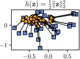
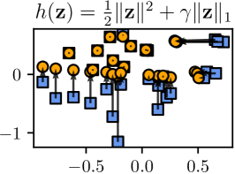
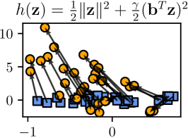
Figure 1: Illustration of ground truth optimal transport maps with different costs $h$, for the same base function $f$. Here we take for $f(\mathbf{z})=-\mathbf{z}^{T}W\mathbf{z}+\mathbf{v}^{T}\mathbf{z}$, a concave quadratic function, and compute the optimal transport map $T_{f}^{h}$ following Prop. 2 using different base costs. On the left, with the usual $\ell_{2}^{2}$ cost, the map simply corresponds to a linear map. With a sparsity-inducing cost (middle), we obtain sparse displacements: most arrows follow the canonical axes. On the right, we take a cost that has a stronger penalization in the direction of a vector $\mathbf{b}$. We see that the displacements mostly align in a direction that is orthogonal to $\mathbf{b}$. This idea is at the core of our proposal to learn structured costs for Monge displacements (Section 4.1).

We propose to deep-dive in this section on optimal transport maps induced by the family of costs in Equation 5. We consider first the practical computation of $h$-transforms for an arbitrary potential function $f$ and arbitrary structured penalty $\tau$. This approach is useful for two reasons: it provides a way to define ground-truth Monge maps for structured costs $h$, answering positively a question raised in the last pages of (Cuturi et al., 2023) on our ability to generate ground-truth structured OT maps. In addition to that result, we also show that the $h$-transform of entropic maps results in a convex problem, a result that we use directly to follow the hyperparameter tuning approach outlined by Vacher and Vialard (2022).

3.1 On the computation of $h$-concave potentials and ground truth $h$-transports

We explore how to compute the $h$-transform, defined in Equation 3, of a potential function $f$. The minimization of $\bar{f}^{h}$ can be done using proximal gradient descent with step-size $\lambda>0$ when $f$ is concave and smooth and when $\mathrm{prox}_{\lambda h}$ is available, following the iterations:

$$\mathbf{x}\xleftarrow{}\mathbf{y}+\mathrm{prox}_{\lambda h}(\mathbf{x}-\mathbf{y}+\lambda\nabla f(\mathbf{x})).$$ (11)

Running these iterations, we obtain the $h$-transform of $f$ as well as its gradient. In practice, because $h$ is the sum of a function $\gamma\tau$ and a quadratic term, one has, thanks to (Parikh et al., 2014, §2.1.1), that the proximal operator of $\lambda h$ is given by

$$\operatorname{prox}_{\lambda h}(\mathbf{z})=\operatorname{prox}_{\frac{\lambda\gamma}{\lambda+1}\tau}\left(\frac{\mathbf{z}}{1+\lambda}\right).$$

This observation is summarized in the following proposition:

Proposition 1.

Assume $f$ is $L$-smooth and concave and that $\lambda<2/L$. Then, iterations (11) converge to a point $\mathbf{x}^{\star}(\mathbf{y})=\operatorname*{arg\,min}_{\mathbf{x}}h(\mathbf{x}-\mathbf{y})-f(\mathbf{x})$. Furthermore, we have

$$\bar{f}^{h}(\mathbf{y})=h(\mathbf{x}^{\star}(\mathbf{y})-\mathbf{y})-f(\mathbf{x}^{\star}(\mathbf{y}))\text{, and }\nabla\bar{f}^{h}(\mathbf{y})=-\nabla h(\mathbf{x}^{\star}(\mathbf{y})-\mathbf{y}).$$ (12)

Proof.

The convergence of iterates (11) follows from (Beck and Teboulle, 2009, Theo. 1) or (Rockafellar, 1976, Theo. 1). Bauschke and Combettes (2011, Prop. 18.7) then give the last identities. ∎

Equipped with $h$-concave potentials, we can now define a ground-truth optimal map with respect to general structured costs $h$, which can be used to produce ground-truth OT maps for $h$.

Proposition 2.

Let $\mu$ be a measure and push it forward using $T_{f}^{h}:=\mathrm{Id}-\operatorname{prox}_{\gamma\tau}\circ\nabla\bar{f}^{h}$ then $T_{f}^{h}$ is optimal for cost $h$ between $\mu$ and $(T_{f}^{h})_{\sharp}\mu$.

Proof.

The result follows from (Santambrogio, 2015, Theorem 1.17). ∎

In summary, the proximal operator of $\tau$ is the only thing needed to implement iterations (11), and, as a result, the $h$-transform of a suitable concave potential. We can then plug the solution in (12) to compute the quantities of interest numerically, plugged back again in a proximal operator to compute the pushforward $T_{f}^{h}$. In practice, we use the JAXOPT (Blondel et al., 2021) library to integrate these steps in our differentiable pipeline seamlessly. We illustrate numerically in $2$d the resulting transport maps for different choices of regularizer $\tau$ in Fig. 1. In this illustration, we use the same base function $f$, so we see clearly that the choice of cost has a drastic impact on the form of the transport map.

3.2 Estimation of $\bar{f}_{\varepsilon}^{h}$, the $h$-transform of entropic potentials

As recently established, our goal is to compute optimal transport maps induced by a ground-truth $h$-concave potentials $\bar{f}^{h}$. The difficulty here, of course, lies in obtaining a reliable estimate of $\bar{f}^{h}$. The MBO estimator outlined in Section 2 cements the validity of entropic potentials as computationally efficient surrogates. However, the choice of $\varepsilon$ remains, as a poorly chosen regularization parameter can lead to a useless estimator.

Following the pipeline introduced by Vacher and Vialard (2022), we propose a model selection framework for tuning $\varepsilon$ that relies on the efficient computation of $h$-transforms. For a given candidate potential function $\hat{f}$, Vacher and Vialard (2022) consider the value of the dual problem

$$\mathcal{D}(\hat{f})=\int\hat{f}{\rm{d}}\mu+\int\hat{f}^{h}{\rm{d}}\nu$$ (13)

as a criterion for model selection. However, Vacher and Vialard (2022) only consider the case of $h(\cdot)=\tfrac{1}{2}\|\cdot\|^{2}\,$ where the $h$-transform becomes the Fenchel conjugate operator.

In order to consider more general costs, we make a step towards computing $h$-transforms of entropic potentials by studying the hessian of their objective and show that this can be done efficiently using proximal gradient descent when $h$ is a more general quadratic cost. This is outlined in the following propositions, where we establish convexity and smoothness of these potentials, which is required to use 1.

Proposition 3.

For fixed $y\in\mathbb{R}^{d}$, the Hessian of $x\mapsto h(\mathbf{x}-y)-f_{\varepsilon}(\mathbf{x})$ is given by

$$\nabla^{2}_{xx}h(\mathbf{x})-\mathbb{E}_{\pi_{\varepsilon}}[\nabla^{2}_{xx}h(\mathbf{x}-Y)|X=\mathbf{x}]+\varepsilon^{-1}\mathrm{Cov}_{\pi_{\varepsilon}}[\nabla_{x}h(\mathbf{x}-Y)|X=\mathbf{x}]\,.$$ (14)

The proof can be found in Appendix A. This leads to the following corollary for quadratic costs.

Corollary 1.

Let $(f_{\varepsilon},g_{\varepsilon})$ be optimal entropic potentials for a quadratic cost $h(x-\mathbf{y}):=\tfrac{1}{2}(x-\mathbf{y})^{\top}B(x-\mathbf{y}).$ Then the function $h(\cdot-\mathbf{y})-f_{\varepsilon}$ is convex.

Proof.

Note that $\nabla_{x}h(\mathbf{x}-Y)=B(\mathbf{x}-Y)$, which is linear, and $\nabla^{2}_{x,x}h(\cdot)=B$ is constant in both $x$ and $Y$. Performing the appropriate cancellations, eq. 14 reads

$$\varepsilon^{-1}\mathrm{Cov}_{\pi_{\varepsilon}}[B(\mathbf{x}-Y)|X=\mathbf{x}]\,,$$ (15)

which remains positive semi-definite. ∎

Finally, to compute $\bar{f}_{\varepsilon}^{h}$, control on the smoothness of $f_{\varepsilon}$ is necessary. We claim that if $(f_{\varepsilon},g_{\varepsilon})$ are optimal entropic potentials corresponding to two compactly supported measures $\mu$ and $\nu$, and $h$ is a quadratic cost, then $f_{\varepsilon}$ is smooth with parameter $O(\varepsilon^{-1})$, as a direct consequence of Vacher and Vialard (2022, Proposition 5). The following result, whose proof can be found in Appendix A, proposes sufficient conditions on $\mathbf{y}$ so that $\bar{f}_{\varepsilon}^{h}(\mathbf{y})$ is well defined.

Proposition 4.

Consider $f_{\varepsilon}$ computed using Eq. (9). If the cost $h$ is convex and $\mathbf{y}$ is in the convex hull of the $\mathbf{y}_{j}$’s, then $\bar{f}_{\varepsilon}^{h}(\mathbf{y})>-\infty$. Conversely, if $h$ is quadratic, then $\bar{f}^{h}_{\varepsilon}(\mathbf{y})>-\infty$ implies that $\mathbf{y}$ is in the convex hull of the $\mathbf{y}_{j}$’s. Moreover, if $h$ is Lipschitz continous, then $\bar{f}_{\varepsilon}^{h}(\mathbf{y})>-\infty$ for any $\mathbf{y}$.

3.3 General Dictionaries and Connections to Generalized Lasso

When $A$ is a general dictionary, namely a full-rank matrix $A\in\mathbb{R}^{p\times d}$ with no properties, a closed-form solution is not available. However, the calculations can be done numerically via a proximal gradient algorithm, as done for instance with the generalized LASSO (Ali and Tibshirani, 2019).

Proposition 5.

For a generic matrix $A$ one has $\operatorname{prox}_{\gamma\tau(A\cdot)}(\mathbf{z})=\mathbf{z}-A^{T}\mathbf{d}^{\star},$ where $\mathbf{d}^{\star}$ solves the dual maximization problem $\max_{\mathbf{d}}\tfrac{1}{2}\|\mathbf{z}\|^{2}-\tfrac{1}{2}\|\mathbf{z}-A^{T}\mathbf{d}\|^{2}-\gamma\tau^{*}(\mathbf{d}/\gamma).$

Proof.

The proof follows, by minimizing the objective and applying Fenchel-Rockafellar duality.

$$\min_{\mathbf{w}} \tfrac{1}{2}\|\mathbf{w}-\mathbf{z}\|^{2}+\gamma\tau(A\mathbf{w})=\min_{\mathbf{w},\mathbf{q}:{A\mathbf{w}=\mathbf{q}}}\tfrac{1}{2}\|\mathbf{w}-\mathbf{q}\|^{2}+\gamma\tau(\mathbf{z})$$

$$=\max_{\mathbf{d}}\min_{\mathbf{w},\mathbf{q}}\tfrac{1}{2}\|\mathbf{w}-\mathbf{z}\|^{2}+\gamma\tau(\mathbf{z})+\mathbf{d}^{T}(A\mathbf{w}-\mathbf{q})$$

$$=\max_{\mathbf{d}}-(\|\cdot-\mathbf{z}\|^{2}/2)^{*}(-A^{T}\mathbf{d})-(\gamma\tau)^{*}(\mathbf{d})=\max_{\mathbf{d}}-(\|\cdot-\mathbf{z}\|^{2}/2)^{*}(-A^{T}\mathbf{d})-\gamma\tau^{*}(\mathbf{d}/\gamma)$$

$$=\max_{\mathbf{d}}\tfrac{1}{2}\|\mathbf{z}\|^{2}-\tfrac{1}{2}\|\mathbf{z}-A^{T}\mathbf{d}\|^{2}-\gamma\tau^{*}(\mathbf{d}/\gamma)\enspace.$$

the result follows from optimality conditions and primal/dual relationships. ∎

4 On Learning Structured Costs for Monge Displacements

We propose in this section a practical pipeline to learn the parameters of the regularizer $\tau$, to infer a regularized cost $h$ that captures suitable regularity in displacements.

4.1 On Learning Structured Costs

Let $\tau_{\theta}$ be a parameterized family of regularizers. Our goal is to learn, given input and target measures, a parameter $\theta$ such that the bulk of the transport cost is dominated by displacements with low regularization value. Since the only moving piece in our pipeline will be $\theta$, we consider all other parameters constant and re-write (8) as:

$$P^{\star}(\theta):=P^{\star}\left(\mathbf{X},\mathbf{a},\mathbf{Y},\mathbf{b};\tfrac{1}{2}\ell^{2}_{2}+\gamma\tau_{\theta},\varepsilon\right).$$ (16)

The matrix $P^{\star}(\theta)$ contains $n\times m$ weights that each quantify the association strength between a pair $(\mathbf{x}_{i},\mathbf{y}_{j})$. Such pairs are characterized by a displacement $\mathbf{z}_{ij}:=\mathbf{y}_{j}-\mathbf{x}_{i}$. We expect $P^{\star}(\theta)$ is such that $\mathbf{z}_{ij}$ is well represented by points with a low value for $\tau_{\theta}$. In other words, we expect that $\tau_{\theta}(\mathbf{z}_{ij})$ be as small as possible when $P_{ij}^{\star}(\theta)$ is high. We, therefore, consider the objective function

$$\mathcal{L}(\theta):=\left\langle P^{\star}(\theta),M(\theta)\right\rangle,\text{ with }M\text{ the matrix of entries }[M(\theta)]_{ij}=\tau_{\theta}(\mathbf{z}_{ij}).$$ (17)

Here, $P^{\star}(\theta)$ is itself obtained as the solution to an optimization problem. The problem of minimizing $\mathcal{L}$ is, therefore, a bilevel problem. In order to solve it, we need to be able to compute the gradient $\nabla\mathcal{L}(\theta)$. The chain rule gives

$$\nabla\mathcal{L}(\theta)=M(\theta)\left[\frac{\partial P^{\star}(\theta)}{\partial\theta}\right]+P^{\star}(\theta)\left[\frac{\partial M(\theta)}{\partial\theta}\right].$$ (18)

The first Vector-Jacobian Product (VJP) is computed using the implicit function theorem as $P^{\star}(\theta)$ is the solution to a minimization problem. We rely on OTT-JAX(Cuturi et al., 2022) to compute it efficiently and seamlessly. The second VJP is a classical VJP computed using JAX’s autodiff. Next, we turn to a parametrization $\tau_{\theta}$ allowing us to learn a subspace on which the displacements lie.

4.2 Subspace Structured Costs

Recall that for a rank-$p$ matrix $A\in\mathbb{R}^{p\times d}$, $p\leq d$, the projection matrix that maps it to its orthogonal is $A^{\perp}=I-A^{T}(AA^{T})^{-1}A$. When $A$ lies in the Stiefel manifold (i.e. $AA^{T}=I$), we have the simplification $A^{\perp}=I-A^{T}A$. This results in the Pythagorean identity $\|\mathbf{z}\|^{2}=\|A^{\perp}\mathbf{z}\|^{2}+\|A\mathbf{z}\|^{2}$, as intended. In order to promote displacements that happen within the span of $A$, we must set a regularizer that penalizes the presence of $\mathbf{z}$ within its complement:

$$\tau_{A^{\perp}}(\mathbf{z}):=\tfrac{1}{2}\|A^{\perp}\mathbf{z}\|^{2}_{2}=\tfrac{1}{2}\mathbf{z}^{T}(A^{\perp})^{T}A^{\perp}\mathbf{z}=\tfrac{1}{2}\mathbf{z}^{T}(I_{d}-A^{T}(AA^{T})^{-1}A)\mathbf{z}.$$

Since $\tau_{A^{\perp}}$ is evidently a quadratic form, its proximal operator can be obtained by solving a linear system (Parikh et al., 2014, §6.1.1); developing and using the matrix inversion lemma results in

$$\operatorname{prox}_{\gamma\tau_{{A^{\perp}}}}(\mathbf{z})=\left(I_{d}+\gamma(A^{\perp})^{T}A^{\perp}\right)^{-1}\mathbf{z}=\tfrac{1}{1+\gamma}(I+\gamma A^{T}(AA^{T})^{-1}A)\,\mathbf{z}.$$ (19)

To summarize, given an orthogonal sub-basis $A$ of $p$ vectors (each of size $d$), promoting that a vector $\mathbf{z}$ lies in its orthogonal can be achieved by regularizing its norm in the orthogonal of $A$. That norm has a proximal operator that can be computed either by

1. Parameterizing $A$ implicitly, through an explicit parameterization of an orthonormal basis $B$ for $A^{\perp}$, as a matrix directly specified in the $(d-p)\times p$ Stiefel manifold. This can alleviate computations to obtain a closed form for its proximal operator:

   $$\operatorname{prox}_{\gamma\tau_{A^{\perp}}}(\mathbf{z})=\operatorname{prox}_{\gamma\tau_{B}}(\mathbf{z})=\mathbf{z}-B^{T}\left(B\mathbf{z}-\frac{1}{1+\gamma}B\mathbf{z}\right)=\left(I_{d}-\frac{\gamma}{1+\gamma}B^{T}B\right)\mathbf{z},$$

   but requires storing $B$, a $(d-p)\times d$ orthogonal matrix, which is cumbersome when $p\ll d$.

2. Parameterizing $A$ explicitly, either as a full-rank $p\times d$ matrix, or more simply a $p\times d$ orthogonal matrix, to recover the suitable proximal operator for $\tau_{A^{\perp}}$, by either

   1. Falling back on the right-most expression in (20) in the linear solve, which can be handled using sparse conjugate gradient solvers, since the application of the right-most linear operator has complexity $(p+1)\times d$ and is positive definite, in addition to the linear solve of complexity $O(p^{3})$. This is of course much simplifies when $A$ is orthogonal, $A\in\mathcal{S}_{p,d}$ since in that case,

      $$\operatorname{prox}_{\gamma\tau_{{A^{\perp}}}}(\mathbf{z})=\frac{1}{1+\gamma}\left(I_{d}+\gamma A^{T}A\right)\mathbf{z}.\\$$ (20)

   2. Alternatively, compute a matrix in the $(d-p)\times p$ Stiefel manifold that spans the same linear space as, through the Gram-Schmidt process (Golub and Van Loan, 2013, p.254) of the $d\times d$ matrix $A^{\perp}$ or rank $d-p$, $B:=\textrm{Gram-Schmidt}(A^{\perp})$, to fall back on the expression above.

We can then use this structured cost in the machinery described in Section 4.1. This way, we learn a matrix $A$ such that displacements between the two target measures happen mostly in the range of $A$. As discussed above, the cost function $\mathcal{L}(A)$ should be optimized over the Stiefel manifold (Edelman et al., 1998). We use Riemannian gradient descent (Boumal, 2023) for this task, which iterates

$$A\xleftarrow{}\mathcal{P}(A-\eta\mathrm{grad}\mathcal{L}(A)),$$

with $\eta>0$ a step size, $\mathrm{grad}\mathcal{L}(A)$ the Riemannian gradient of $\mathcal{L}$, given by the formula $\mathrm{grad}\mathcal{L}(A)=G-AG^{T}A$ with $G=\nabla\mathcal{L}(A)$ the standard Euclidean gradient of $A$ computed with autodiff, and $\mathcal{P}$ the projection on the Stiefel manifold, with formula $\mathcal{P}(A)=(AA^{\top})^{-1/2}A$. The Euclidean gradient of $\mathcal{L}$ is computed using the IFT as described after Eq. (18). As proposed by Absil and Malick (2012), we use projections to stay on the manifold.

5 Statistical Aspects of Subspace Monge Maps

The costs proposed in the second part of Section 4 are designed to encourage the displacements of the transport maps to lie in a particular subspace of $\mathbb{R}^{d}$. In this section, we consider the statistical complexity of estimating such maps from data. The question of estimating transport maps was first studied in a statistical context by Hütter and Rigollet (2021), and subsequent research has proposed alternative estimation procedures, with different statistical and computational properties (Deb et al., 2021; Manole et al., 2021; Muzellec et al., 2021; Pooladian and Niles-Weed, 2021). We extend this line of work by considering the analogous problem for Monge maps with structured displacements.

We show that with a proper choice of $\varepsilon$, the MBO estimator defined by (10) is a consistent estimator of $T^{\star}$ as $n\to\infty$, and prove a rate of convergence in $L^{2}(\mu)$. We also give preliminary theoretical evidence that, as $\gamma\to\infty$, maps corresponding to the subspace structured cost $\frac{1}{2}\ell_{2}^{2}+\gamma\tau_{A^{\perp}}$ can be estimated at a rate that depends only on the subspace dimension $p$, rather than on the ambient dimension $d$, thereby avoiding the curse of dimensionality.

5.1 Sample complexity estimates for the MBO estimator

The MBO estimator is a generalization of the entropic map estimator, originally defined by Pooladian and Niles-Weed (2021) for the quadratic cost $h=\frac{1}{2}\ell_{2}^{2}$. This estimator has been statistically analyzed in several regimes, see e.g., Pooladian et al. (2023); Rigollet and Stromme (2022); del Barrio et al. (2022) and Goldfeld et al. (2022). We show that this procedure also succeeds for subspace structured costs of the form $h=\frac{1}{2}\ell_{2}^{2}+\gamma\tau_{A^{\perp}}$. As a result of being recast as an estimation task for quadratic cost, the following sample-complexity result for the MBO estimator follows from (Pooladian and Niles-Weed, 2021, Theorem 3), and a computation relating the MBO estimator to a barycentric projection for the costs we consider (see Appendix B for the full statements and proofs).

Theorem 1.

Let $A\in\mathbb{R}^{p\times d}$ be fixed, and consider $\tilde{T}$ given by an $M$-smooth and $m$-strongly convex function, with smooth inverse, and suppose $\mu$ has an upper and lower bounded density with compact support, and $\nu$ is lower-bounded. Consider $T^{\star}$ of the form eq. 23 for some $\gamma\geq 0$ fixed, and suppose we have samples $X_{1},\ldots,X_{n}\sim\mu$ and $Y_{1},\ldots,Y_{n}\sim(T^{\star})_{\sharp}\mu$. Let $\hat{T}_{\varepsilon}$ be the MBO estimator with $\varepsilon\asymp n^{-\frac{1}{d^{\prime}+4}}$. Then it holds that

$$\mathbb{E}\|\hat{T}_{\varepsilon}-T^{\star}\|^{2}_{L^{2}(\mu)}\lesssim n^{-\frac{2}{d^{\prime}+4}}\,,$$

where $d^{\prime}=2\lceil d/2\rceil$, where the underlying constants depend on properties of $\mu,\nu,\tilde{T},\gamma$ and $A$.

5.2 Connection to the Spiked Transport Model

The additional structure we impose on the displacements allows us to closely relate our model to the “spiked transport model" as defined in Niles-Weed and Rigollet (2022), see also (Paty and Cuturi, 2019; Lin et al., 2020, 2021a). The authors studied the estimation of the Wasserstein distance in the setting where the Brenier map between $\mu$ and $\nu$ takes the form,

$$T_{\text{spiked}}(\mathbf{x})=\mathbf{x}-A^{T}(A\mathbf{x}-S(A\mathbf{x}))\,,$$ (21)

where $A\in\mathcal{S}_{p,d}$ and $S:\mathbb{R}^{p}\to\mathbb{R}^{p}$ is the gradient of a convex function on $\mathbb{R}^{p}$. Divol et al. (2022) performed a statistical analysis of the map estimation problem under the spiked transport model. They constructed an estimator $\hat{T}_{n}$ such that the $L^{2}(\mu)$ risk decays with respect to the intrinsic dimension $p\ll d$; this is summarized in the following theorem.

Theorem 2.

(Divol et al., 2022, Theorem 3 with Proposition 4) Suppose $\tilde{T}$ is bi-Lipschitz (smooth, and strongly convex) and $\mu$ has compact support, with density bounded above and below. Suppose further that there exists a matrix $A\in\mathbb{R}^{p\times d}$ on the Stiefel manifold such that $\nu:=(T_{\text{spiked}})_{\sharp}\mu$, with $T_{\text{spiked}}$ defined as in eq. 21. Assume that $\mu$ is known explicitly. Given $n$ i.i.d. samples from $\nu$, there exists an estimator $\hat{T}_{n}$ satisfying

$$\mathbb{E}\|\hat{T}_{n}-T_{\text{spiked}}\|^{2}_{L^{2}(\mu)}\lesssim_{\log(n)}n^{-\frac{2}{p}}\,.$$ (22)

We now argue that the spiked transport model can be recovered in the large $\gamma$ limit of subspace structured costs. Indeed, if $\gamma\to\infty$, then displacements in the subspace orthogonal to $A$ are heavily disfavored, so that the optimal coupling will concentrate on the subspace given by $A$, thereby recovering a map of the form (21), which by Theorem 2 can be estimated at a rate independent of the ambient dimension. Making this observation quantitative by characterizing the rate of estimation of $T^{\star}$ as a function of $\gamma$ for $\gamma$ large is an interesting question for future work.

6 Experiments

We study with two synthetic tasks in this experimental study. Because of our ability to propose ground-truth $h$-optimal maps, we can now benchmark the MBO estimator in the simplest settings when $h$ is known, and has the general structure considered in this work.

The entire pipeline described in § 4 was implemented by creating a new family of parameterized RegTICost in OTT-JAX(Cuturi et al., 2022). This cost family can be fed into the Sinkhorn solver, and their solution cast solutions as DualPotentials objects that hold holds $f_{\varepsilon}$ for a given $h$. The application of the transport is then recovered using simply automatic differentiation.

6.1 On the MBO Performance For A Synthetic Ground Truth Displacement

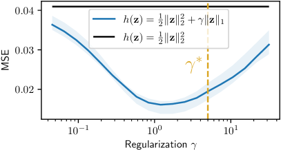
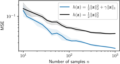
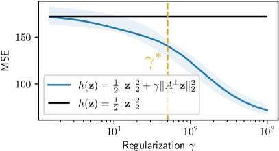
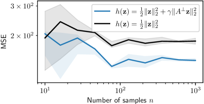
Figure 2: Performance of the MBO estimator on two ground-truth tasks involving the $\tau=\ell_{1}$ (top row) and $\tau_{A^{\perp}}=\|A^{\perp}\mathbf{z}\|^{2}_{2}$ (bottom row) structured costs, where $p=2$ in dimension $5$. $\gamma^{*}$ is the level of regularization used for the ground truth in data generation, whereas performance are shown varying w.r.t $\gamma$. Knowing the cost (not its strength) does help in these experiments in the estimation of transport map.

In this section, we assume that the cost structure is known, using the same $\tau$ both for generation and estimation, except for regularization strength $\gamma$. We use that cost to evaluate the transport associated with $\bar{f}_{\varepsilon}^{h}$ on a sample of points, using Proposition2, and then compare the performance of Sinkhorn based estimators, either with that cost or the standard $\tfrac{1}{2}\ell^{2}_{2}$ cost (which corresponds to $\gamma=0$).

We consider the $\tau=\ell_{1}$ and $\tau_{A^{\perp}}=\|A^{\perp}\mathbf{z}\|^{2}_{2}$ regularizer, and its associated proximal soft-thresholding operator. To estimate OT, we assume that we do not know $\gamma$ (we do not use directly $\gamma^{*}$) and vary it, reporting mean-squared error of predictions.

We first sample a random quadratic function $f(\mathbf{z}):=\frac{1}{2}(\mathbf{z}-\mathbf{w})^{T}M(\mathbf{z}-\mathbf{w})$ where $M$ is a Wishart matrix, sampled as $M=QQ^{T}$, with $Q\in\mathbb{R}^{d\times 2d}$ is multivariate Gaussian, and $\mathbf{w}$ is a random Gaussian vector. We then sample $n=200$ Gaussian points in dimension $d=5$ and push them through the transport associated with $\bar{f}_{\varepsilon}^{h}$, to recover matched train data $\mathbf{Y}_{T}$ and $\mathbf{X}_{T}$, and do the same for a test fold $\mathbf{Y}_{t}$ and $\mathbf{X}_{t}$ of the same size, to report our metric, the MSE. The MSE is defined, given an estimator for $f$ and its associated cost function $h$,as $\|T_{f_{\varepsilon,\gamma}}(\mathbf{X}_{t})-\mathbf{Y}_{t}\|^{2}_{2}$. We plot this MSE as a function of $\gamma$, where $\gamma=0$ would correspond exactly to the $\ell_{2}^{2}$ cost. We observe in Figure 2, that our estimator outperforms significantly the $\ell_{2}^{2}$ pipeline for any range of the parameter $\gamma$. Here, the projection dimension $p=2$ , and data dimension $d=5$.

6.2 Learning Subspace from Synthetic Displacement

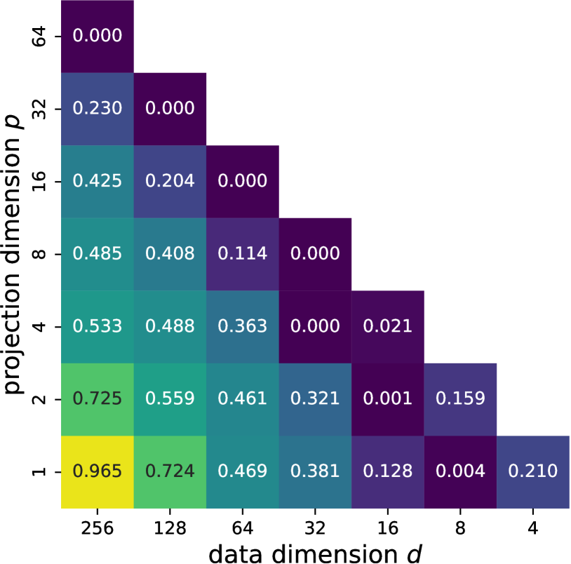
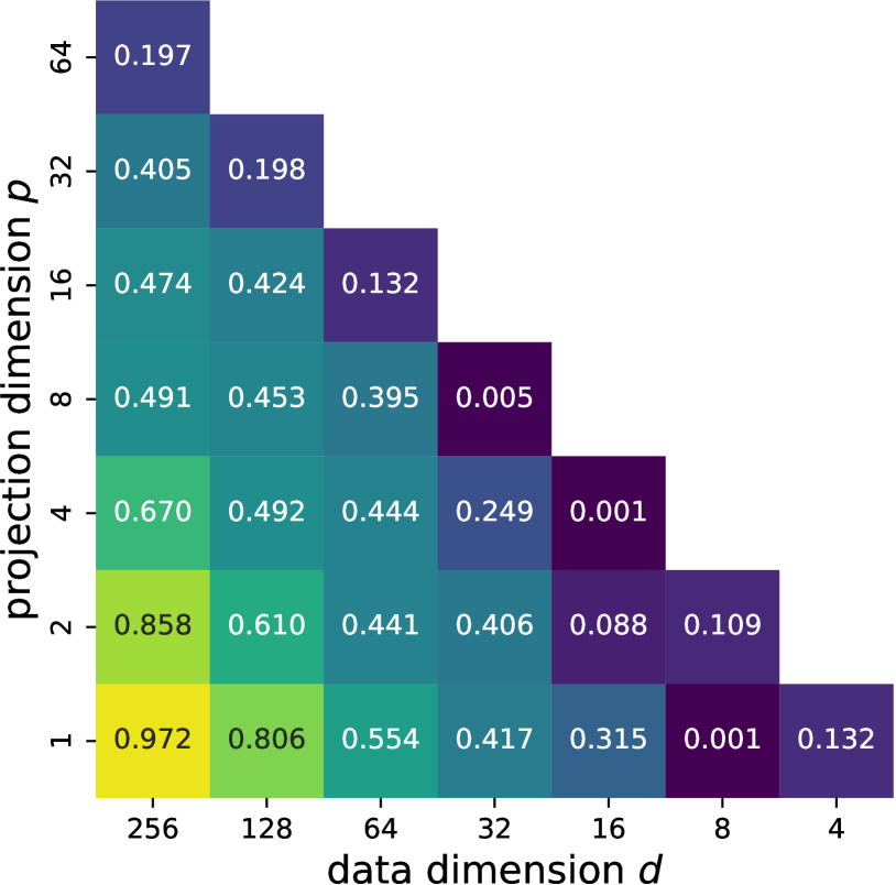
Figure 3: Recovery (error) of parameters of $p\times d$ cost matrices depending on dimension, using gradient descent. The values displayed represent squared-residual errors when projecting the $p$ ground truth basis vectors $A^{*}$ onto the $2p$ orthogonal vectors of $\hat{A}$, our estimator for the cost. Left corresponds to setting $\gamma$ regularization to obtain $80\%$ of inertia in $p^{*}$ dimensions, while right corresponds to $90\%$.

We propose to test the ability of our pipeline to recover a ground truth $A^{*}$ parameter within a squared-Euclidean cost. To do so, we proceed as follows. For dimension $d$, we build our $h$ function by selecting $A^{*}$ by sampling a $p^{*}\times d$ normal matrix that is projected on the $p^{*}\times d$ Stiefel manifold.

As in the previous section, we sample a random quadratic function $f(\mathbf{z}):=\frac{1}{2}\mathbf{z}^{T}M\mathbf{z}$, sample a point cloud $\mathbf{X}$ of $n=512$ standard Gaussian points, and apply, following Proposition2, the corresponding ground-truth transport to obtain $\mathbf{Y}$ of the same size. We set the regularization parameter $\gamma$ manually, such that the $p^{*}$ first singular values of displacements $\mathbf{Y}-\mathbf{X}$ capture either 80% or 90% of the total inertia, ensuring that most displacements are indeed captured by $p^{*}$ directions.

We then launch our solver with a dimension $\hat{p}=2p^{*}$, and measure our recovery for $\hat{A}$ by looking at the average (normalized by basis size) of the residual error, when projecting the vectors in $A^{*}$ in the orthogonal basis $\hat{A}$, namely $\|A^{*}-\hat{A}\hat{A}^{T}A^{*}\|_{2}^{2}/p^{*}$. For simplicity, we use an iteration $i$ stepsize of $2/\sqrt{i}$. These results in Figure 3 highlight the phenomenon that larger $p^{*}$ seem to be easier to recover.

Conclusion.

We propose in this paper an algorithmic mechanism to design ground-truth transports for structured costs. We exploit this to benchmark successfully the MBO estimator on two tasks, involving the $\ell_{1}$ and an orthogonal projection norm. These experiments showcase the versatility of the MBO framework. Additionally, we propose an inverse OT problem in which the goal is to learn the parameters of a regularizer. Intuitively, our aim is to learn a regularizer parameter, such that the OT displacements it promotes, have themselves low regularization values. We explored this approach by learning a subspace for displacements (and not, as considered previously, for the entire pointclouds) and provided encouraging recovery results.

Appendix A Proofs from Section 3

Proof of 3.

Recall $f_{\varepsilon}(\mathbf{x})=\min_{\varepsilon}[h(\mathbf{x}-\mathbf{y})-g_{\varepsilon}(\mathbf{y})]$. Taking the gradient under the integral, we arrive at

$$\nabla f_{\varepsilon}(\mathbf{x})=\frac{\int\nabla_{x}h(\mathbf{x}-y)e^{(g_{\varepsilon}(\mathbf{y})-h(\mathbf{x}-y))/\varepsilon}{\rm{d}}Q(\mathbf{y})}{\int e^{(g_{\varepsilon}(\mathbf{y})-h(\mathbf{x}-y))/\varepsilon}{\rm{d}}Q(\mathbf{y})}\,.$$

We apply the quotient rule for vector-valued functions. Writing $\nabla f_{\varepsilon}(\mathbf{x})=\mathbb{A}/e^{-f_{\varepsilon}(\mathbf{x})/\varepsilon},$ where the denominator is valid by the marginal conditions, we write

$$\nabla^{2}f_{\varepsilon}(\mathbf{x})=\frac{\nabla\mathbb{A}}{e^{-f_{\varepsilon}(\mathbf{x})/\varepsilon}}-\left(\frac{\nabla e^{-f_{\varepsilon}(\mathbf{x})/\varepsilon}}{e^{-f_{\varepsilon}(\mathbf{x})/\varepsilon}}\right)\otimes\left(\frac{\mathbb{A}}{e^{-f_{\varepsilon}(\mathbf{x})}}\right)\,.$$

We compute the remaining terms:

$$\nabla\mathbb{A}=\int\left[\nabla^{2}_{xx}h(\mathbf{x}-y)-\varepsilon^{-1}\nabla_{x}h(\mathbf{x}-y)^{\otimes 2}\right]e^{(g_{\varepsilon}(\mathbf{y})-h(\mathbf{x}-y))/\varepsilon}{\rm{d}}Q(\mathbf{y})\,.$$

Also,

$$\frac{\nabla e^{-f_{\varepsilon}(\mathbf{x})/\varepsilon}}{e^{-f_{\varepsilon}(\mathbf{x})/\varepsilon}}=-\frac{1}{\varepsilon}\nabla f_{\varepsilon}(\mathbf{x})=-\frac{1}{\varepsilon}\frac{\mathbb{A}}{e^{-f_{\varepsilon}(\mathbf{x})/\varepsilon}}\,.$$

Recognizing the conditional entropic plan $\pi_{\varepsilon}^{x}(\mathbf{y})=e^{(f_{\varepsilon}(\mathbf{x})+g_{\varepsilon}(\mathbf{y})-h(\mathbf{x}-y))/\varepsilon}{\rm{d}}Q(\mathbf{y})$ we obtain the following expression for the Hessian

$$\nabla^{2}f_{\varepsilon}(\mathbf{x})=\mathbb{E}_{\pi_{\varepsilon}}[\nabla^{2}_{xx}h(\mathbf{x}-Y)|X=\mathbf{x}]-\varepsilon^{-1}\mathrm{Cov}_{\pi_{\varepsilon}}[\nabla_{x}h(\mathbf{x}-Y)|X=\mathbf{x}]\,.$$

∎

Proof of 4.

The problem is that of knowing whether

$$\phi_{\mathbf{y}}(\mathbf{x}):=h(\mathbf{x}-\mathbf{y})+\varepsilon\log\sum\exp((-h(\mathbf{x}-\mathbf{y}_{j})+\beta_{j})/\varepsilon)$$

is lower bounded or not. Simple manipulations give

$$\phi_{\mathbf{y}}(\mathbf{x})=\varepsilon\log\sum\exp((h(\mathbf{x}-\mathbf{y})-h(\mathbf{x}-\mathbf{y}_{j})+\beta_{j})/\varepsilon)$$

which is lower bounded if for any $\mathbf{x}$, it exists $j$ such that $h(\mathbf{x}-\mathbf{y})-h(\mathbf{x}-\mathbf{y}_{j})+\beta_{j}>-\infty$. By convexity of $h(\mathbf{x}-\cdot)$ and for $g_{\mathbf{x}}(\mathbf{y}_{j})\in\partial h(\mathbf{x}-\cdot)(\mathbf{y}_{j})$, this holds if $\langle g_{\mathbf{x}}(\mathbf{y}_{j}),\mathbf{y}-\mathbf{y}_{j}\rangle<+\infty$ which holds with the stronger assumption that $\mathbf{y}$ in the convex hull of $\mathbf{y}_{j}$ for any direction $d$: $\langle d,\mathbf{y}-\mathbf{y}_{j}\rangle\leq 0$. This condition is also necessary when $h(\mathbf{x})=\langle\mathbf{x},M\mathbf{x}\rangle$ for some positive symmetric matrix $M$. If $h$ is $L$-Lipschitz continuous, we have $\|g_{x}(y_{j})\|\leq L$ and then from Cauchy-Schwartz inequality

$$\langle g_{\mathbf{x}}(\mathbf{y}_{j}),\mathbf{y}-\mathbf{y}_{j}\rangle\leq L\|y-y_{j}\|<+\infty.$$

∎

Appendix B Proofs from Section 5

To perform this analysis, we rely on the following characterization of optimal maps for subspace structured costs, which reveals a close connection with optimal maps for the standard $\ell_{2}^{2}$ cost.

Proposition 6.

Let $T^{\star}$ be the optimal map between $\mu$ and $\nu$ for the cost $h=\tfrac{1}{2}\ell_{2}^{2}+\gamma\tau_{A^{\perp}}.$ Denote by $W$ the linear map $\mathbf{x}\mapsto((1+\gamma)I-\gamma A^{T}A)^{1/2}\mathbf{x}$. Then $W\circ T^{\star}\circ W^{-1}$ is the Brenier map (i.e., $\ell_{2}^{2}$ optimal map) between $W_{\sharp}\mu$ and $W_{\sharp}\nu$. Equivalently, $T^{\star}$ is $h$-optimal if and only if it can be written

$$T^{\star}=W^{-1}\circ\tilde{T}\circ W,$$ (23)

where $\tilde{T}$ is the gradient of a convex function.

Proof of 6.

The cost $h=\frac{1}{2}\ell_{2}^{2}+\gamma\tau_{A^{\perp}}$ can be written as

$$\tfrac{1}{2}\left[z^{\top}(I+\gamma(A^{\perp})^{\top}A^{\perp})z\right]=\tfrac{1}{2}\|Wz\|^{2}\,.$$

The optimal transport problem we consider is therefore equivalent to minimizing

$$\min_{\pi\in\Gamma(\mu,\nu)}\int\tfrac{1}{2}\|Wx-Wy\|^{2}{\rm{d}}\pi(x,y)=\min_{\pi\in\Gamma(W_{\sharp}\mu,W_{\sharp}\nu)}\int\tfrac{1}{2}\|x^{\prime}-y^{\prime}\|^{2}{\rm{d}}\pi(x^{\prime},y^{\prime})\,.$$ (24)

Brenier’s theorem implies that the solution to the latter problem is given by the gradient of a convex function, and that this property uniquely characterizes the optimal map. Writing this function as $\tilde{T}$, we obtain that the optimal coupling between $W_{\sharp}\mu$ and $W_{\sharp}\nu$ is given by $y^{\prime}=\tilde{T}(x^{\prime})$, which implies that the optimal $h$-coupling between $\mu$ and $\nu$ is given by $T^{\star}=W^{-1}\circ\tilde{T}\circ W$, as desired.

∎

The proof of 1 requires the following two lemmas.

Lemma 1.

For costs of the form $h(z)=\tfrac{1}{2}z^{\top}Bz$ where $B$ is positive definite, the MBO estimator between two measures $\mu$ and $\nu$ can be written as the barycentric projection of the corresponding optimal entropic coupling.

Proof.

Note that $h^{*}(w)=\tfrac{1}{2}w^{\top}B^{-1}w$, and thus $\nabla h^{*}(w)=B^{-1}w$. Let $(f_{\varepsilon},g_{\varepsilon})$ denote the optimal entropic potentials for this cost, with corresponding coupling $\pi_{\varepsilon}$. Borrowing computations from Appendix A, we know that

$$\nabla f_{\varepsilon}(x)=\int B(x-y){\rm{d}}\pi_{\varepsilon}^{x}(y)=Bx-B\int y{\rm{d}}\pi_{\varepsilon}^{x}(y)\,,$$

where $\pi_{\varepsilon}^{x}(y)$ is the conditional entropic coupling (given $x$). The proof concludes by taking the expression of the MBO estimator and expanding:

$$T_{\varepsilon}(x)=x-(\nabla h^{*})\circ(\nabla f_{\varepsilon}(x))=x-B^{-1}\left(Bx-B\int y{\rm{d}}\pi_{\varepsilon}^{x}(y)\right)=\int y{\rm{d}}\pi_{\varepsilon}^{x}(y)\,,$$

which is the definition of the barycentric projection of $\pi_{\varepsilon}$ for a given $x$. ∎

Lemma 2 (Pre-conditioning of MBO).

Let $T_{\varepsilon}$ be the MBO estimator between $\mu$ and $\nu$ for the cost $h=\tfrac{1}{2}\ell^{2}+\gamma\tau_{A^{\perp}}$. Let $W$ be denoted as in 6. Then the MBO estimator is written as

$$T_{\varepsilon}=W^{-1}\circ\tilde{T}_{\varepsilon}\circ W\,,$$ (25)

where $\tilde{T}_{\varepsilon}$ is the barycentric projection between $W_{\sharp}\mu$ and $W_{\sharp}\nu$.

Proof.

The proof here is similar to 6, which we outline again for completeness. As before, we are interested in solutions to the optimization problem

$$\min_{\pi\in\Gamma(\mu,\nu)}\int\tfrac{1}{2}\|Wx-Wy\|^{2}{\rm{d}}\pi(x,y)+\varepsilon\text{KL}(\pi\|\mu\otimes\nu)\,,$$

with optimal coupling $\pi_{\varepsilon}^{\star}$. Performing a change of variables $\pi^{\prime}=(W\otimes W)_{\sharp}\pi$, we have

$$\min_{\pi^{\prime}\in\Gamma(\mu^{\prime},\nu^{\prime})}\int\tfrac{1}{2}\|x-y\|^{2}{\rm{d}}\pi^{\prime}(x,y)+\varepsilon\text{KL}(\pi^{\prime}\|\mu^{\prime}\otimes\nu^{\prime})\,,$$

where $\mu^{\prime}:=W_{\sharp}\mu$ (and similarly for $\nu^{\prime}$), where now the optimizer reads $(\pi_{\varepsilon}^{\prime})^{\star}$. The two optimal plans are related as

$$\pi^{\star}=(W^{-1}\otimes W^{-1})_{\sharp}(\pi_{\varepsilon}^{\prime})^{\star}\,.$$

It was established in 1 that the MBO estimator $T^{\star}_{\varepsilon}$ is given by the barycentric projection

$$T_{\varepsilon}^{\star}(x)=\mathbb{E}_{\pi_{\varepsilon}^{\star}}[Y|X=x]\,.$$

Performing the change of variables $Y^{\prime}=WY$ and $X^{\prime}=WX$, we can re-write this as a function of $\pi^{\prime}_{\varepsilon}$ instead:

$$T^{\star}_{\varepsilon}(x) =\mathbb{E}_{\pi_{\varepsilon}^{\star}}[Y|X=x]$$

$$=\mathbb{E}_{(\pi_{\varepsilon}^{\prime})^{\star}}[W^{-1}Y^{\prime}|W^{-1}X^{\prime}=x]$$

$$=W^{-1}\mathbb{E}_{(\pi_{\varepsilon}^{\prime})^{\star}}[Y^{\prime}|X^{\prime}=Wx]$$

$$=W^{-1}\tilde{T}_{\varepsilon}(Wx)\,,$$

where we identify $\tilde{T}_{\varepsilon}(\cdot):=\mathbb{E}_{(\pi_{\varepsilon}^{\prime})^{\star}}[Y^{\prime}|X^{\prime}=\cdot]$; this completes the proof. ∎

We are now ready to present the main proof.

Proof of 1.

Let $T_{\varepsilon,n}$ denote the MBO estimator between samples from $\mu$ and $\nu$, and let $\tilde{T}_{\varepsilon,n}$ denote the entropic map estimator from samples $\mu^{\prime}:=W_{\sharp}\mu$ and $\nu^{\prime}:=W_{\sharp}\nu$, where $W$ has spectrum $0<\lambda_{\min}(W)\leq\lambda_{\max}(W)<+\infty$, where we have access to $W$ since $A$ is known.

Our goal is to establish upper bounds on

$$\|T_{\varepsilon,n}-T^{\star}\|^{2}_{L^{2}(\mu)}=\|W^{-1}\circ(\tilde{T}_{\varepsilon,n}\circ W-\tilde{T}\circ W)\|^{2}_{L^{2}(\mu)}\,.$$

Paying for constants that scale like $\lambda_{\max}(W^{-1})$, we have the bound

$$\|T_{\varepsilon,n}-T^{\star}\|^{2}_{L^{2}(\mu)}\lesssim_{W}\|\tilde{T}_{\varepsilon,n}-\tilde{T}\|^{2}_{L^{2}(\mu^{\prime})}\,,$$

where we can now directly use the rates of convergence from [Pooladian and Niles-Weed, 2021, Theorem 3], as $\mu^{\prime}$ satisfies our regularity assumptions under the conditions we have imposed on $W$. this completes the proof. ∎

Appendix C Additional experiments in the spirit of Figure 2

In this section we add a few experiments, in the spirit of Figure 2.

We follow the same setup as in that figure, but we do explore a few changes in parameters such as number of train/test points $n$, dimension $d$ of points, as well as projection dimension $p$.

Depending on the dimension and the order of magnitude of data, the range for a relevant regularization strength parameter $\gamma$ might vary. By relevant, we mean, for instance, that it is strong enough to enforce sparsity (for the case $\tau=\|\cdot\|_{1}$) or to enforce that displacements are overwhelmingly happening in a subspace $A$ (for the case $\tau=\|A^{\perp}\cdot\|^{2}_{2}$).

In these experiments, and unlike Figure 2, we do not choose a predefined value for $\gamma^{\star}$, but instead select it with the following procedure: we start with a small value for $\gamma_{0}=0.1$, and increase it gradually, until a certain desirable criterion on these displacements goes above a threshold. To measure this, we first compute the (paired) matrix of displacements on a given sample,

$$D=[T_{f}^{h}(\mathbf{x}_{i})-\mathbf{x}_{i}]_{i}\in\mathbb{R}^{n\times d}$$

We then consider average sparsity (to select $\gamma$ for $\|\cdot\|_{1}$),

$$\textrm{sp}(\gamma)=\tfrac{1}{nd}\sum_{i,j=1}^{n,d}\mathbf{1}(D_{ij}<0.0001)\in[0,1]\,.$$ (26)

We consider ratio of singular values on $p$ subspace (to select $\gamma$ for $\|A^{\perp}\cdot\|^{2}_{2}$), writing $\sigma$ for the vector of singular values of $D$, ranked in decreasing order, to compute

$$\textrm{sv-ratio}(\gamma)=\sum_{i=1}^{p}\sigma_{i}/\sum_{i}\sigma_{i}\in[0,1]\,.$$ (27)

We pick two $\gamma$’s in experiments for Figure 6 and  5, such that their criterion is just above a low value of $0.2$ (low relative regularization) and $0.8$ (high relative regularization). We expect our MBO estimators to outperform “more” the $\ell_{2}$ MBO in the latter (high regularization) regime. In Figure 4 we only select one $\gamma^{\star}$ for a criterion for each setup corresponding to $0.8$. Error bars are computed using 10 regenerations of data samples.

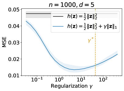
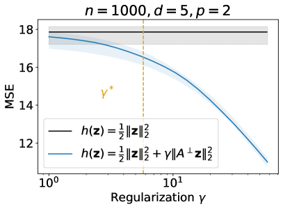
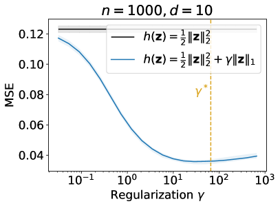
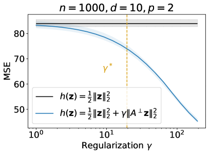
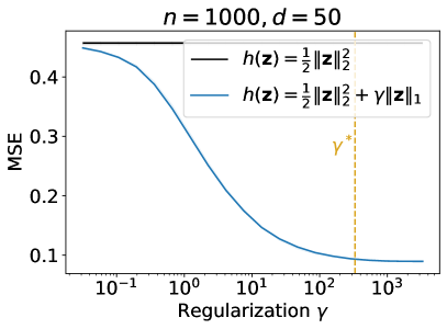
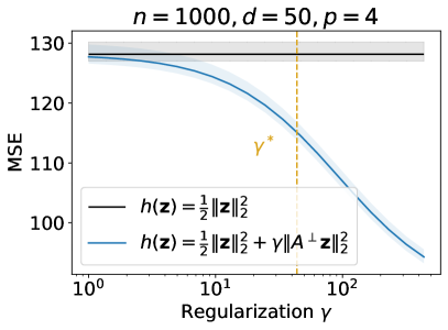
Figure 4: Experiments with both $\|\cdot\|_{1}$ and $\|A^{\perp}\|^{2}_{2}$ regularizers. Here $\gamma$ varies, and can be smaller or higher than the ground truth parameter $\gamma^{\star}$ used to generate data. That ground truth regularization strength $\gamma^{\star}$ is selected to ensure that the mean sparsity on the left (resp. svd ratio of top $p$ singular values for $\|A^{\perp}\|^{2}_{2}$ on the right) of displacements is higher than 80% . The number of points $n$ is fixed, and $d$ increases from top to bottom.

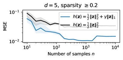
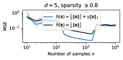
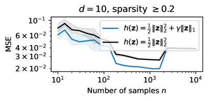
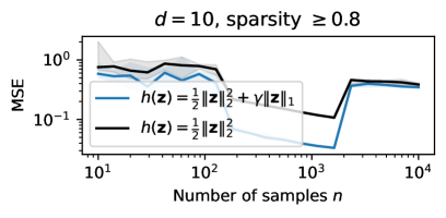
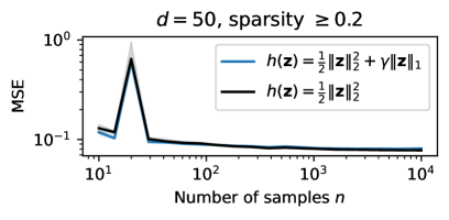
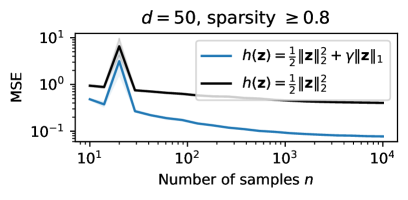
Figure 5: Experiments with the $\|\cdot\|_{1}$ regularizer. Here $\gamma$ used in estimation corresponds to the ground truth $\gamma^{\star}$ selected to ensure mean sparsity pattern of displacements (see (26)) is higher than 20% (left) or 80% (right). Ambient dimension $d$ (and $p$ for projections on right column) varies from top to bottom.

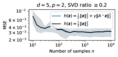
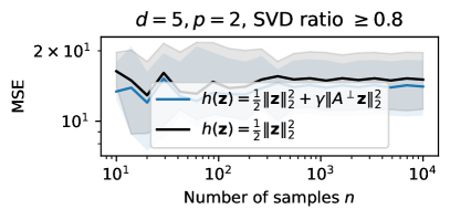
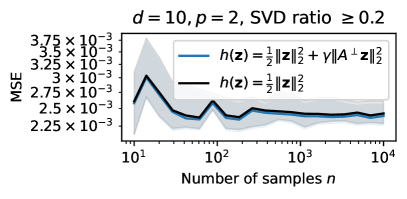
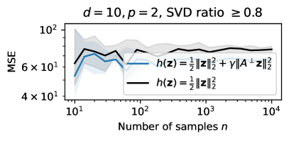
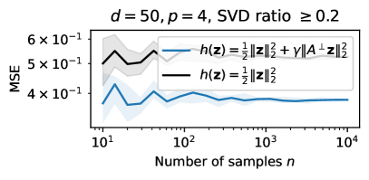
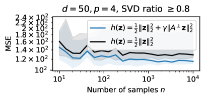
Figure 6: Experiments with the $\|A^{\perp}\cdot\|_{2}^{2}$ regularizer, as in Fig.5. The criterion now used is the SVD ratio (see (27)).

References

- Absil and Malick (2012) P-A Absil and Jérôme Malick. Projection-like retractions on matrix manifolds. SIAM Journal on Optimization, 22(1):135–158, 2012.
- Ali and Tibshirani (2019) Alnur Ali and Ryan J Tibshirani. The generalized lasso problem and uniqueness. Electronic Journal of Statistics, 13:2307–2347, 2019.
- Amos et al. (2017) Brandon Amos, Lei Xu, and J Zico Kolter. Input Convex Neural Networks. volume 34, 2017.
- Bauschke and Combettes (2011) Heinz H Bauschke and Patrick L Combettes. Convex analysis and monotone operator theory in Hilbert spaces, volume 408. Springer, 2011.
- Beck and Teboulle (2009) Amir Beck and Marc Teboulle. A fast iterative shrinkage-thresholding algorithm for linear inverse problems. SIAM journal on imaging sciences, 2(1):183–202, 2009.
- Blondel et al. (2021) Mathieu Blondel, Quentin Berthet, Marco Cuturi, Roy Frostig, Stephan Hoyer, Felipe Llinares-López, Fabian Pedregosa, and Jean-Philippe Vert. Efficient and modular implicit differentiation. arXiv preprint arXiv:2105.15183, 2021.
- Bonneel et al. (2015) Nicolas Bonneel, Julien Rabin, Gabriel Peyré, and Hanspeter Pfister. Sliced and radon wasserstein barycenters of measures. Journal of Mathematical Imaging and Vision, 51:22–45, 2015.
- Boumal (2023) Nicolas Boumal. An introduction to optimization on smooth manifolds. Cambridge University Press, 2023.
- Brenier (1991) Yann Brenier. Polar factorization and monotone rearrangement of vector-valued functions. Communications on Pure and Applied Mathematics, 44(4), 1991. doi: 10.1002/cpa.3160440402.
- Bunne et al. (2021) Charlotte Bunne, Stefan G. Stark, Gabriele Gut, Jacobo Sarabia del Castillo, Kjong-Van Lehmann, Lucas Pelkmans, Andreas Krause, and Gunnar Rätsch. Learning single-cell perturbation responses using neural optimal transport. bioRxiv, 2021. doi: 10.1101/2021.12.15.472775.
- Bunne et al. (2022) Charlotte Bunne, Andreas Krause, and Marco Cuturi. Supervised training of conditional monge maps. In S. Koyejo, S. Mohamed, A. Agarwal, D. Belgrave, K. Cho, and A. Oh, editors, Advances in Neural Information Processing Systems, volume 35, pages 6859–6872. Curran Associates, Inc., 2022.
- Caron et al. (2021) Mathilde Caron, Hugo Touvron, Ishan Misra, Hervé Jégou, Julien Mairal, Piotr Bojanowski, and Armand Joulin. Emerging properties in self-supervised vision transformers. In Proceedings of the IEEE/CVF international conference on computer vision, 2021.
- Courty et al. (2017) Nicolas Courty, Rémi Flamary, Amaury Habrard, and Alain Rakotomamonjy. Joint distribution optimal transportation for domain adaptation. Advances in Neural Information Processing Systems, 30, 2017.
- Cuturi (2013) Marco Cuturi. Sinkhorn distances: Lightspeed computation of optimal transport. In Advances in neural information processing systems, pages 2292–2300, 2013.
- Cuturi et al. (2022) Marco Cuturi, Laetitia Meng-Papaxanthos, Yingtao Tian, Charlotte Bunne, Geoff Davis, and Olivier Teboul. Optimal transport tools (ott): A jax toolbox for all things wasserstein. arXiv preprint arXiv:2201.12324, 2022.
- Cuturi et al. (2023) Marco Cuturi, Michal Klein, and Pierre Ablin. Monge, bregman and occam: Interpretable optimal transport in high-dimensions with feature-sparse maps. In Proceedings of the 40th ICML, 2023.
- Dalalyan (2017) Arnak S Dalalyan. Theoretical guarantees for approximate sampling from smooth and log-concave densities. Journal of the Royal Statistical Society. Series B (Statistical Methodology), pages 651–676, 2017.
- Deb et al. (2021) Nabarun Deb, Promit Ghosal, and Bodhisattva Sen. Rates of estimation of optimal transport maps using plug-in estimators via barycentric projections. arXiv preprint arXiv:2107.01718, 2021.
- del Barrio et al. (2022) Eustasio del Barrio, Alberto Gonzalez-Sanz, Jean-Michel Loubes, and Jonathan Niles-Weed. An improved central limit theorem and fast convergence rates for entropic transportation costs. arXiv preprint arXiv:2204.09105, 2022.
- Deshpande et al. (2019) Ishan Deshpande, Yuan-Ting Hu, Ruoyu Sun, Ayis Pyrros, Nasir Siddiqui, Sanmi Koyejo, Zhizhen Zhao, David Forsyth, and Alexander G Schwing. Max-sliced wasserstein distance and its use for gans. In Proceedings of the IEEE/CVF Conference on Computer Vision and Pattern Recognition, pages 10648–10656, 2019.
- Divol et al. (2022) Vincent Divol, Jonathan Niles-Weed, and Aram-Alexandre Pooladian. Optimal transport map estimation in general function spaces. arXiv preprint arXiv:2212.03722, 2022.
- Dudley et al. (1966) Richard Mansfield Dudley et al. Weak convergence of probabilities on nonseparable metric spaces and empirical measures on euclidean spaces. Illinois Journal of Mathematics, 10(1):109–126, 1966.
- Edelman et al. (1998) Alan Edelman, Tomás A Arias, and Steven T Smith. The geometry of algorithms with orthogonality constraints. SIAM journal on Matrix Analysis and Applications, 20(2):303–353, 1998.
- Goldfeld et al. (2022) Ziv Goldfeld, Kengo Kato, Gabriel Rioux, and Ritwik Sadhu. Limit theorems for entropic optimal transport maps and the sinkhorn divergence. arXiv preprint arXiv:2207.08683, 2022.
- Golub and Van Loan (2013) Gene H Golub and Charles F Van Loan. Matrix computations. JHU press, 2013.
- Huang et al. (2021) Minhui Huang, Shiqian Ma, and Lifeng Lai. A riemannian block coordinate descent method for computing the projection robust wasserstein distance. In Proceedings of the 38th International Conference on Machine Learning, volume 139 of Proceedings of Machine Learning Research, pages 4446–4455. PMLR, 2021.
- Hütter and Rigollet (2021) Jan-Christian Hütter and Philippe Rigollet. Minimax estimation of smooth optimal transport maps. The Annals of Statistics, 49(2), 2021.
- Janati et al. (2020) Hicham Janati, Thomas Bazeille, Bertrand Thirion, Marco Cuturi, and Alexandre Gramfort. Multi-subject meg/eeg source imaging with sparse multi-task regression. NeuroImage, 2020.
- Kolouri et al. (2019) Soheil Kolouri, Kimia Nadjahi, Umut Simsekli, Roland Badeau, and Gustavo Rohde. Generalized sliced wasserstein distances. Advances in neural information processing systems, 32, 2019.
- Korotin et al. (2019) Alexander Korotin, Vage Egiazarian, Arip Asadulaev, Alexander Safin, and Evgeny Burnaev. Wasserstein-2 generative networks. 2019.
- Korotin et al. (2021) Alexander Korotin, Lingxiao Li, Aude Genevay, Justin Solomon, Alexander Filippov, and Evgeny Burnaev. Do Neural Optimal Transport Solvers Work? A Continuous Wasserstein-2 Benchmark. 2021.
- Le et al. (2019) Tam Le, Makoto Yamada, Kenji Fukumizu, and Marco Cuturi. Tree-sliced variants of wasserstein distances. Advances in neural information processing systems, 32, 2019.
- Lin et al. (2020) Tianyi Lin, Chenyou Fan, Nhat Ho, Marco Cuturi, and Michael Jordan. Projection robust wasserstein distance and riemannian optimization. Advances in neural information processing systems, 33:9383–9397, 2020.
- Lin et al. (2021a) Tianyi Lin, Zeyu Zheng, Elynn Chen, Marco Cuturi, and Michael Jordan. On projection robust optimal transport: Sample complexity and model misspecification. In Arindam Banerjee and Kenji Fukumizu, editors, Proceedings of The 24th International Conference on Artificial Intelligence and Statistics, volume 130 of Proceedings of Machine Learning Research, pages 262–270. PMLR, 13–15 Apr 2021a. URL https://proceedings.mlr.press/v130/lin21a.html.
- Lin et al. (2021b) Tianyi Lin, Zeyu Zheng, Elynn Chen, Marco Cuturi, and Michael I Jordan. On projection robust optimal transport: Sample complexity and model misspecification. In International Conference on Artificial Intelligence and Statistics, pages 262–270. PMLR, 2021b.
- Makkuva et al. (2020) Ashok Makkuva, Amirhossein Taghvaei, Sewoong Oh, and Jason Lee. Optimal transport mapping via input convex neural networks. volume 37, 2020.
- Manole et al. (2021) Tudor Manole, Sivaraman Balakrishnan, Jonathan Niles-Weed, and Larry Wasserman. Plugin estimation of smooth optimal transport maps. arXiv preprint arXiv:2107.12364, 2021.
- Monge (1781) Gaspard Monge. Mémoire sur la théorie des déblais et des remblais. Histoire de l’Académie Royale des Sciences, 1781.
- Muzellec et al. (2021) Boris Muzellec, Adrien Vacher, Francis Bach, François-Xavier Vialard, and Alessandro Rudi. Near-optimal estimation of smooth transport maps with kernel sums-of-squares. arXiv preprint arXiv:2112.01907, 2021.
- Niles-Weed and Rigollet (2022) Jonathan Niles-Weed and Philippe Rigollet. Estimation of wasserstein distances in the spiked transport model. Bernoulli, 28(4):2663–2688, 2022.
- Oquab et al. (2023) Maxime Oquab, Timothée Darcet, Théo Moutakanni, Huy Vo, Marc Szafraniec, Vasil Khalidov, Pierre Fernandez, Daniel Haziza, Francisco Massa, Alaaeldin El-Nouby, et al. Dinov2: Learning robust visual features without supervision. arXiv preprint arXiv:2304.07193, 2023.
- Parikh et al. (2014) Neal Parikh, Stephen Boyd, et al. Proximal algorithms. Foundations and trends® in Optimization, 1(3):127–239, 2014.
- Paty and Cuturi (2019) François-Pierre Paty and Marco Cuturi. Subspace robust wasserstein distances. arXiv preprint arXiv:1901.08949, 2019.
- Peyré and Cuturi (2019) Gabriel Peyré and Marco Cuturi. Computational optimal transport. Foundations and Trends® in Machine Learning, 11, 2019.
- Pooladian and Niles-Weed (2021) Aram-Alexandre Pooladian and Jonathan Niles-Weed. Entropic estimation of optimal transport maps. arXiv preprint arXiv:2109.12004, 2021.
- Pooladian et al. (2023) Aram-Alexandre Pooladian, Vincent Divol, and Jonathan Niles-Weed. Minimax estimation of discontinuous optimal transport maps: The semi-discrete case. arXiv preprint arXiv:2301.11302, 2023.
- Rabin et al. (2012) Julien Rabin, Gabriel Peyré, Julie Delon, and Marc Bernot. Wasserstein barycenter and its application to texture mixing. In Scale Space and Variational Methods in Computer Vision: Third International Conference, pages 435–446. Springer, 2012.
- Rigollet and Stromme (2022) Philippe Rigollet and Austin J Stromme. On the sample complexity of entropic optimal transport. arXiv preprint arXiv:2206.13472, 2022.
- Rockafellar (1976) R Tyrrell Rockafellar. Monotone operators and the proximal point algorithm. SIAM journal on control and optimization, 14(5):877–898, 1976.
- Salimans et al. (2018) Tim Salimans, Han Zhang, Alec Radford, and Dimitris Metaxas. Improving GANs using optimal transport. In International Conference on Learning Representations, 2018.
- Sander et al. (2022) Michael E Sander, Pierre Ablin, Mathieu Blondel, and Gabriel Peyré. Sinkformers: Transformers with doubly stochastic attention. In International Conference on Artificial Intelligence and Statistics. PMLR, 2022.
- Santambrogio (2015) Filippo Santambrogio. Optimal transport for applied mathematicians. Springer, 2015.
- Schiebinger et al. (2019) Geoffrey Schiebinger, Jian Shu, Marcin Tabaka, Brian Cleary, Vidya Subramanian, Aryeh Solomon, Joshua Gould, Siyan Liu, Stacie Lin, Peter Berube, et al. Optimal-transport analysis of single-cell gene expression identifies developmental trajectories in reprogramming. Cell, 176(4):928–943, 2019.
- Sinkhorn (1964) Richard Sinkhorn. A relationship between arbitrary positive matrices and doubly stochastic matrices. Ann. Math. Statist., 35:876–879, 1964.
- Tay et al. (2020) Yi Tay, Dara Bahri, Liu Yang, Donald Metzler, and Da-Cheng Juan. Sparse Sinkhorn attention. In Proceedings of the 37th International Conference on Machine Learning, volume 119 of Proceedings of Machine Learning Research. PMLR, 13–18 Jul 2020.
- Tong et al. (2020) Alexander Tong, Jessie Huang, Guy Wolf, David Van Dijk, and Smita Krishnaswamy. TrajectoryNet: A dynamic optimal transport network for modeling cellular dynamics. In Proceedings of the 37th International Conference on Machine Learning, volume 119 of Proceedings of Machine Learning Research, pages 9526–9536. PMLR, 2020.
- Vacher and Vialard (2022) Adrien Vacher and François-Xavier Vialard. Parameter tuning and model selection in optimal transport with semi-dual brenier formulation. In Alice H. Oh, Alekh Agarwal, Danielle Belgrave, and Kyunghyun Cho, editors, Advances in Neural Information Processing Systems, 2022.
- Vincent-Cuaz et al. (2023) Cédric Vincent-Cuaz, Rémi Flamary, Marco Corneli, Titouan Vayer, and Nicolas Courty. Semi-relaxed gromov-wasserstein divergence and applications on graphs. In International Conference on Learning Representations, 2023.
- Weed and Bach (2019) Jonathan Weed and Francis Bach. Sharp asymptotic and finite-sample rates of convergence of empirical measures in wasserstein distance. Bernoulli, 25(4A), 2019.