Quantum theory of non-hermitian optical binding between nanoparticles

Abstract

Recent experiments demonstrate highly tunable non-reciprocal coupling between levitated nanoparticles due to optical binding [Rieser et al., Science 377, 987 (2022)]. In view of recent experiments cooling nanoparticles to the quantum regime, we here develop the quantum theory of small dielectric objects interacting via the forces and torques induced by scattered tweezer photons. The interaction is fundamentally non-hermitian and accompanied by correlated quantum noise. We present the corresponding Markovian quantum master equation, show how to reach non-reciprocal and unidirectional coupling, and identify unique quantum signatures of optical binding. Our work provides the theoretical tools for exploring and exploiting the rich quantum physics of non-reciprocally coupled nanoparticle arrays.

I Introduction

Optically levitated nanoparticles in vacuum offer a promising table-top platform for probing and exploiting quantum physics with massive objects Gonzalez-Ballestero et al. (2021); Stickler et al. (2021). The ability to continuously monitor their dynamics, to precisely control their motion and rotation, and to let co-levitated particles interact strongly in a highly tunable fashion promises a plethora of future applications in science and technology. State-of-the-art setups cool the center-of-mass motion of a single particle into its quantum ground state Delić et al. (2020); Magrini et al. (2021); Tebbenjohanns et al. (2021); Ranfagni et al. (2022); Kamba et al. (2022); Piotrowski et al. (2023) and rotational degrees of freedom to millikelvin temperatures Bang et al. (2020); Delord et al. (2020); van der Laan et al. (2021); Pontin et al. (2023). Levitated sensors achieve force and torque sensitivities on the order of $10^{-21}$ Newton Ranjit et al. (2016); Hempston et al. (2017); Liang et al. (2023); Zhu et al. (2023) and $10^{-27}$ Newtonmeter Ahn et al. (2020), which will likely be improved further in future experiments. This may enable the detection of high-frequency gravitational waves Arvanitaki and Geraci (2013); Aggarwal et al. (2022) and tests of physics beyond the standard model Moore and Geraci (2021); Carney et al. (2021); Afek et al. (2022); Yin et al. (2022). In addition, levitated nanoparticles may well allow exploring the quantum-to-classical transition at high masses Bateman et al. (2014); Wan et al. (2016); Pino et al. (2018), probing yet unobserved quantum interference phenomena in the rotational degrees of freedom Stickler et al. (2018); Ma et al. (2020); Schrinski et al. (2022), detecting non-classical correlations in arrays of massive objects Rudolph et al. (2020); Brandão et al. (2021); Rudolph et al. (2022); Chauhan et al. (2022), and demonstrating entanglement via Newtonian gravity Bose et al. (2017); Marletto and Vedral (2017).

Trapping and controlling multiple objects in optical arrays is core to many future applications of levitated nanoparticles Afek et al. (2022); Rieser et al. (2022); Brzobohaty et al. (2023); Penny et al. (2023); Vijayan et al. (2023). The interference of the light scattered off one particle with the field trapping the others can give rise to strong interactions between them, commonly referred to as optical binding Burns et al. (1989); Karásek et al. (2006); Dholakia and Zemánek (2010). Most experiments thus far focused on a regime where the interparticle coupling can be described as effectively conservative Mohanty et al. (2004); Dholakia and Zemánek (2010); Svak et al. (2021); Liska et al. (2023). However, optical binding is known to exhibit non-reciprocal behaviour Ostermann et al. (2014); Sukhov et al. (2015), which seemingly violates Newton’s third law. The recent study Rieser et al. (2022) demonstrated full tunability between reciprocal and non-reciprocal optical binding of equally sized particles, establishing levitated nanoparticles as a viable setup for realizing non-hermitian physics Ashida et al. (2020); Okuma and Sato (2023). Paradigmatic examples of effectively non-hermitian dynamics include directional amplification Wanjura et al. (2020); Wang et al. (2022) and topological phase transitions Shen et al. (2018); Bergholtz et al. (2021); Kawabata et al. (2023), with potential applications for sensing Lau and Clerk (2018); De Carlo et al. (2022).

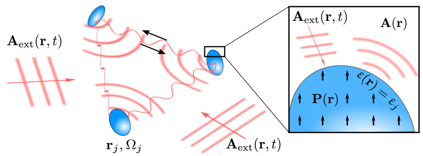
Figure 1: Several nanoparticles with center-of-mass position $\mathbf{r}_{j}$, orientation $\Omega_{j}$, and dielectric constant $\upvarepsilon_{j}$ are illuminated by a laser field $\mathbf{A}_{\rm ext}(\mathbf{r},t)$. The latter induces a polarization field $\mathbf{P}(\mathbf{r})$, oscillating in phase with the laser field and leading to dipole radiation $\mathbf{A}(\mathbf{r})$ known as Rayleigh scattering. The interference of the scattered fields with the incoming laser field gives rise to the optical-binding interaction between the particles, which may be non-reciprocal and unidirectional.

A quantum description of non-reciprocal interactions requires accounting for the fact that the two coupled partices experience correlated quantum noises Kepesidis et al. (2016); Metelmann and Clerk (2017); Lau and Clerk (2018); Zhang et al. (2019). In the case of optical binding we show that the corresponding common bath Clerk (2022) is provided by the electromagnetic vacuum field surrounding the particles. Field quantization in the presence of multiple dielectrics is complicated by the fact that the total field, comprised of the incident laser and scattered radiation, must be self-consistent with the induced polarization densities, which in turn depend on the position and orientation of all particles. Solving the resulting integral equation in the Rayleigh limit of small dielectrics, we derive a Markovian quantum master equation for the coupled quantum mechanical dynamics of an arbitrary number of nanoparticles interacting via light scattering. This framework generalizes the classically observed non-reciprocal interactions Rieser et al. (2022) and predicts unique signatures of quantum optical binding in terms of correlated quantum noises. We show how quantum optical binding can be probed and tuned in state-of-the experiments, paving the way for exploring and exploiting non-hermitian quantum physics and topologically nontrivial phases in large nanoparticle arrays.

The remainder of the article is structured as follows: Section II derives the quantized interaction between an arbitrary number of small dielectrics illuminated by multiple lasers and their electromagnetic environment. In Sec. III, we obtain the optical-binding quantum master equation for the particle motion by tracing out the electromagnetic vacuum. This equation is simplified in Sec. IV for an array of deeply trapped nanoparticles to study the effects of correlated quantum noise and the prospects for entanglement generation and for unidirectional quantum transport. We discuss possible generalizations of our work in Sect. V, and provide the quantum Langevin equations of optical binding as well as technical details in the Appendices.

II Light-matter interaction

II.1 Lagrange function

To facilitate consistent canonical quantization of several particles interacting via the electrodynamic field, we first consider the combined classical dynamics of dielectric matter with relative permittivity tensor $\upvarepsilon({\bf r})$ and of the electromagnetic field. The polarization field $\mathbf{P}(\mathbf{r})$ determines the density of bound charges $\rho_{\rm P}(\mathbf{r})=-\nabla\cdot\mathbf{P}(\mathbf{r})$ in the dielectric. These charges give rise to a longitudinal electric field as characterized by the electrostatic dipole Green tensor

$${\sf G}_{0}(\mathbf{r})=\frac{3\mathbf{r}\otimes\mathbf{r}-r^{2}\mathbb{1}}{4\pi r^{5}},$$ (1)

where $r=|\mathbf{r}|$. In the absence of free charges, the total electric field ${\bf E}({\bf r})$ is the sum of the resulting instantaneous dipole field and of the transverse electric field, for instance due to a laser. Denoting by $\mathbf{A}_{\rm tot}(\mathbf{r})$ the vector potential in Coulomb gauge, $\nabla\cdot\mathbf{A}_{\rm tot}(\mathbf{r})=0$, the electric field reads

$$\mathbf{E}(\mathbf{r})=-\partial_{t}\mathbf{A}_{\rm tot}(\mathbf{r})+\frac{1}{\varepsilon_{0}}\int d^{3}\mathbf{r}^{\prime}{\sf G}_{0}(\mathbf{r}-\mathbf{r}^{\prime})\mathbf{P}(\mathbf{r}^{\prime}).$$ (2)

For linear dielectrics, the internal polarization field is related to the total electric field through the constitutive relation

$$\mathbf{P}(\mathbf{r})=\varepsilon_{0}[\upvarepsilon(\mathbf{r})-\mathbb{1}]\mathbf{E}(\mathbf{r}).$$ (3)

In the following, we assume the dielectric tensor to be dispersion-free and real-valued, as applicable for light scattering off low-absorption media. Inserting $\mathbf{P}(\mathbf{r})$ into Eq. (2), yields an integral equation for the total electric field, which is solved by

$$\mathbf{E}(\mathbf{r})=-\int d^{3}\mathbf{r}^{\prime}{\sf L}(\mathbf{r},\mathbf{r}^{\prime})\partial_{t}\mathbf{A}_{\rm tot}(\mathbf{r}^{\prime}),$$ (4)

where the tensor-valued kernel fulfills

$${\sf L}(\mathbf{r},\mathbf{r}^{\prime}) =\delta(\mathbf{r}-\mathbf{r}^{\prime})\mathbb{1}$$

$$+ \int d^{3}\mathbf{s}\,{\sf G}_{0}(\mathbf{r}-\mathbf{s})[\upvarepsilon(\mathbf{s})-\mathbb{1}]{\sf L}(\mathbf{s},\mathbf{r}^{\prime}).$$ (5)

The uniqueness of its solution is guaranteed by Maxwell’s equations if localized dielectrics are considered and if natural boundary conditions are assumed. The kernel ${\sf L}(\mathbf{r},\mathbf{r}^{\prime})$ satisfies the symmetry relation $[\upvarepsilon(\mathbf{r})-\mathbb{1}]{\sf L}(\mathbf{r},\mathbf{r}^{\prime})={\sf L}^{T}(\mathbf{r}^{\prime},\mathbf{r})[\upvarepsilon(\mathbf{r}^{\prime})-\mathbb{1}]$.

From Eq. (3) the polarization field follows as

$$\mathbf{P}(\mathbf{r})=-\varepsilon_{0}\int d^{3}\mathbf{r}^{\prime}{\sf K}(\mathbf{r},\mathbf{r}^{\prime})\partial_{t}\mathbf{A}_{\rm tot}(\mathbf{r}^{\prime}),$$ (6)

with the integral kernel ${\sf K}(\mathbf{r},\mathbf{r}^{\prime})=[\upvarepsilon(\mathbf{r})-\mathbb{1}]{\sf L}(\mathbf{r},\mathbf{r}^{\prime})$. It describes the induced electrostatic interaction between different volume elements and relates the transverse part of the field to the polarization field. The kernel vanishes outside the dielectrics, where $\upvarepsilon({\bf r})=1$, it is symmetric ${\sf K}(\mathbf{r},\mathbf{r}^{\prime})={\sf K}^{T}(\mathbf{r}^{\prime},\mathbf{r})$, and fulfills the integral equation

$${\sf K}(\mathbf{r},\mathbf{r}^{\prime})= [\upvarepsilon(\mathbf{r})-\mathbb{1}]\delta(\mathbf{r}-\mathbf{r}^{\prime})$$

$$+ [\upvarepsilon(\mathbf{r})-\mathbb{1}]\int d^{3}\mathbf{s}\,{\sf G}_{0}(\mathbf{r}-\mathbf{s}){\sf K}(\mathbf{s},\mathbf{r}^{\prime}).$$ (7)

Now we take $\upvarepsilon({\bf r})$ to describe $N$ non-intersecting, rigid dielectric particles of arbitrary shape and size (see Fig 1). Denoting the center-of-mass position of the $j$-th particle by $\mathbf{r}_{j}$ and its orientation by $\Omega_{j}$, given e.g. by Euler angles $\Omega_{j}=(\alpha_{j},\beta_{j},\gamma_{j})$ in the $z$-$y^{\prime}$-$z^{\prime\prime}$-convention, the dielectric tensor can be written as

$$\upvarepsilon(\mathbf{r}) =\mathbb{1}+$$

$$\sum_{j=1}^{N}{\sf R}(\Omega_{j})\Big{[}\upvarepsilon_{j}[{\sf R}^{T}(\Omega_{j})(\mathbf{r}-\mathbf{r}_{j})]-\mathbb{1}\Big{]}{\sf R}^{T}(\Omega_{j}).$$ (8)

Here, the rotation tensors ${\sf R}(\Omega_{j})$ transform from the reference orientation of the $j$-th particle to their principal axes frames so that the dielectric tensors $\upvarepsilon_{j}(\mathbf{r})$ describe the individual particles in the body fixed frame. The integral kernels ${\sf K}(\mathbf{r},\mathbf{r}^{\prime})$ and ${\sf L}(\mathbf{r},\mathbf{r}^{\prime})$ thus depend on the center-of-mass positions and the orientation of all particles.

The total force $\mathbf{F}_{j}$ and the total torque $\mathbf{N}_{j}$ acting on the $j$-th particle follow from integrating the Lorentz force density over the particle volume ${\cal V}_{j}={\cal V}_{j}({\bf r}_{j},\Omega_{j})$ (see Appendix A),

$$\mathbf{F}_{j}=\int_{\mathcal{V}_{j}}d^{3}\mathbf{r}\,\nabla^{\prime}[\mathbf{P}(\mathbf{r})\cdot\mathbf{E}(\mathbf{r}^{\prime})]_{\mathbf{r}^{\prime}=\mathbf{r}}$$ (9a)

and

$$\mathbf{N}_{j}= \int_{\mathcal{V}_{j}}d^{3}\mathbf{r}\,\mathbf{P}(\mathbf{r})\times\mathbf{E}(\mathbf{r})$$

$$+(\mathbf{r}-\mathbf{r}_{j})\times\nabla^{\prime}[\mathbf{P}(\mathbf{r})\cdot\mathbf{E}(\mathbf{r}^{\prime})]_{\mathbf{r}^{\prime}=\mathbf{r}}.$$ (9b)

Note that the gradients in Eqs. (9a) and (9) act only on the electric field, reflecting that the potential energy of a polarized volume element $$d^{3}\mathbf{r} \mathbf{P}(\mathbf{r})d^{3}\mathbf{r} -\mathbf{P}(\mathbf{r})\cdot\mathbf{E}(\mathbf{r})d^{3}\mathbf{r}$$ with constant dipole moment is . The first term in Eq. (9) is the intrinsic torque on each volume element, describing the precession of the dipole density in the electric field, while the second term is caused by the force density acting on the particle, inducing an orbital torque around the particle center of mass.

These equations are complemented by the wave equation of the transverse vector potential sourced by the transverse part of the polarization current density $\partial_{t}\mathbf{P}(\mathbf{r})$ Jackson (1999),

$$\left(\frac{1}{c^{2}}\partial_{t}^{2}-\Delta\right)\mathbf{A}_{\rm tot}(\mathbf{r})=\mu_{0}\partial_{t}\mathbf{P}_{\perp}(\mathbf{r}).$$ (9c)

The equations of motion (9) can be formulated as Euler-Lagrange equations with Lagrangian

$$L_{\rm tot}=L_{\rm m}+L_{\rm em}^{\rm tot}+L_{\rm int}.$$ (10)

Here, $L_{\rm m}$ denotes the free mechanical Lagrangian of all particles, including their translational and rotational kinetic energies as well as possible external potentials. The free electromagnetic Lagrangian of the transverse electromagnetic field Schubert and Weber (1993) reads

$$L_{\rm em}^{\rm tot}=\int d^{3}\mathbf{r}\left(\frac{\varepsilon_{0}}{2}\left[\partial_{t}\mathbf{A}_{\rm tot}(\mathbf{r})\right]^{2}-\frac{1}{2\mu_{0}}\left[\nabla\times\mathbf{A}_{\rm tot}(\mathbf{r})\right]^{2}\right).$$ (11)

Finally, the light-matter interaction is accounted for by

$$L_{\rm int}=\frac{\varepsilon_{0}}{2}\int d^{3}\mathbf{r}d^{3}\mathbf{r}^{\prime}\left[\partial_{t}\mathbf{A}_{\rm tot}(\mathbf{r})\right]\cdot{\sf K}(\mathbf{r},\mathbf{r}^{\prime})\left[\partial_{t}\mathbf{A}_{\rm tot}(\mathbf{r}^{\prime})\right].$$ (12)

Note that this can be understood as the energy of the polarization field in the transverse electric field characterized by the energy density $\mathbf{P}(\mathbf{r})\cdot\partial_{t}\mathbf{A}_{\rm tot}(\mathbf{r})/2$.

The above derivation assumes rigid dielectrics, which move and revolve on a timescale slow compared to the light propagation through them. Extending this treatment to include other mechanical degrees of freedom, such as elasto-mechanic deformations of the bodies, is conceptually straight-forward. The resulting Lagrangian takes the form Eq. (10), but with the integral kernel depending also on additional generalized coordinates.

The fact that the interaction Lagrangian (12) describes the the full light-matter coupling will prove crucial for quantizing the theory in the small particle limit. This coupling term differs from that typically used for levitated particles Romero-Isart et al. (2011); Stickler et al. (2016a); Gonzalez-Ballestero et al. (2019), even though the difference becomes relevant only when considering more than a single particle.

II.2 Euler-Lagrange equations

We now confirm that the Lagrangian (10) yields the equations of motion (9) for rigid objects. This means that the forces (9a) must be given by

$${\bf F}_{j}=\partial_{{\bf r}_{j}}L_{\rm int}.$$ (13)

The derivative on the right-hand side acts only on the integral kernel ${\sf K}(\mathbf{r},\mathbf{r}^{\prime})$. Denoting its $\ell$-th cartesian component by $({\bf e}_{\ell}\cdot\partial_{\mathbf{r}_{j}})$, we first use that

$$({\bf e}_{\ell}\cdot\partial_{\mathbf{r}_{j}})[\upvarepsilon(\mathbf{r})-\mathbb{1}]=\begin{cases}-\nabla_{\ell}[\upvarepsilon(\mathbf{r})-\mathbb{1}]&{\rm for}\quad{\bf r}\in{\cal V}_{j}\\ 0&{\rm elsewhere.}\end{cases}$$ (14)

Then, in order to evaluate $({\bf e}_{\ell}\cdot\partial_{\mathbf{r}_{j}}){\sf L}(\mathbf{r},\mathbf{r}^{\prime})$ we apply the derivative to Eq. (II.1) and solve the latter,

$$({\bf e}_{\ell}\cdot\partial_{\mathbf{r}_{j}}){\sf L}(\mathbf{r},\mathbf{r}^{\prime})= \int d^{3}\mathbf{s}^{\prime}d^{3}\mathbf{s}\,{\sf L}(\mathbf{r},\mathbf{s}^{\prime}){\sf G}_{0}(\mathbf{s}^{\prime}-\mathbf{s})({\bf e}_{\ell}\cdot\partial_{\mathbf{r}_{j}})$$

$$[\upvarepsilon(\mathbf{s})-\mathbb{1}]{\sf L}(\mathbf{s},\mathbf{r}^{\prime}).$$ (15)

Integration by parts and identifying the integral kernels (II.1) and (II.1) finally leads to

$${\bf e}_{\ell}\cdot\partial_{{\bf r}_{j}}L_{\rm int}= \varepsilon_{0}\int d^{3}\mathbf{s}^{\prime}d^{3}\mathbf{s}\int_{\mathcal{V}_{j}}d^{3}\mathbf{r}\partial_{t}\mathbf{A}_{\rm tot}(\mathbf{s}^{\prime})$$

$$\cdot{\sf K}(\mathbf{s}^{\prime},\mathbf{r})\nabla_{\ell}{\sf L}(\mathbf{r},\mathbf{s})\partial_{t}\mathbf{A}_{\rm tot}(\mathbf{s}),$$ (16)

which demonstrates Eq. (13).

In order to show that the Lagrangian yields the torque (9) we must evaluate the derivative of $L_{\rm int}$ with respect to the Euler angles $\mu_{j}\in\{\alpha_{j},\beta_{j},\gamma_{j}\}$ of the $j$-th particle. We proceed as for the center of mass to obtain

$$\partial_{\mu_{j}}{\sf L}(\mathbf{r},\mathbf{r}^{\prime})= \int d^{3}\mathbf{s}^{\prime}d^{3}\mathbf{s}\,{\sf L}(\mathbf{r},\mathbf{s}^{\prime})$$

$${\sf G}_{0}(\mathbf{s}^{\prime}-\mathbf{s})\partial_{\mu_{j}}[\upvarepsilon(\mathbf{s})-\mathbb{1}]{\sf L}(\mathbf{s},\mathbf{r}^{\prime}).$$ (17)

Using that we can restrict the integration to the $j$-th particle volume yields

$$\partial_{\mu_{j}}L_{\rm int}=\frac{\varepsilon_{0}}{2}\int_{\mathcal{V}_{j}}d^{3}\mathbf{r}\,\mathbf{E}(\mathbf{r})\cdot\partial_{\mu_{j}}[\upvarepsilon(\mathbf{r})-\mathbb{1}]\mathbf{E}(\mathbf{r}),$$ (18)

where the derivative only acts on the dielectric tensor. Using $\partial_{\mu_{j}}{\sf R}(\Omega_{j})=\mathbf{n}_{\mu_{j}}\times{\sf R}(\Omega_{j})$, where $\mathbf{n}_{\mu_{j}}$ is the instantaneous rotation axis associated with $\mu_{j}$, one gets

$$\partial_{\mu_{j}}[\upvarepsilon(\mathbf{r})-\mathbb{1}]= \mathbf{n}_{\mu_{j}}\times[\upvarepsilon(\mathbf{r})-\mathbb{1}]+\Big{[}\mathbf{n}_{\mu_{j}}\times[\upvarepsilon(\mathbf{r})-\mathbb{1}]\Big{]}^{T}$$

$$+[(\mathbf{r}-\mathbf{r}_{j})\cdot(\mathbf{n}_{\mu_{j}}\times\nabla)][\upvarepsilon(\mathbf{r})-\mathbb{1}].$$ (19)

Inserting this into Eq. (18), the first line in Eq. (II.2) yields the intrinsic torque while the second line, after partial integration, yields the torque due to the force density. In total, we thus showed that

$$\partial_{\mu_{j}}L_{\rm int}=\mathbf{n}_{\mu_{j}}\cdot\mathbf{N}_{j},$$ (20)

which is Eq. (9).

Finally, also the right-hand side of the wave equation (9c) must follow from Eq. (12). As $L_{\rm int}$ depends only on the time derivative of the transverse vector potential, we need the functional derivative of $L_{\rm int}$ only with respect to $\partial_{t}\mathbf{A}_{\rm tot}$. Taking the transversality of the vector potential into account, one obtains

$$\partial_{t}\frac{\delta L_{\rm int}}{\delta[\partial_{t}\mathbf{A}_{\rm tot}(\mathbf{r})]}=\varepsilon_{0}\partial_{t}\left(\int d^{3}\mathbf{r}^{\prime}{\sf K}(\mathbf{r},\mathbf{r}^{\prime})\partial_{t}\mathbf{A}_{\rm tot}(\mathbf{r}^{\prime})\right)_{\perp}.$$ (21)

Expressing the right-hand side through the transverse part of the polarization field Eq. (6), one obtains Eq. (9c).

II.3 Small particles in an external field

From now on we assume for simplicity that all arbitrarily shaped particles exhibit a uniform and isotropic permittivity tensor $\varepsilon\mathbb{1}$ and that the particles are much smaller than the distances between them. To treat the inter-particle interactions as a perturbation in the integral kernel (II.1), we first define the integral kernel ${\sf K}_{0}(\mathbf{r},\mathbf{r}^{\prime})$ for the case that all particles are arbitrarily far separated from one another. It fulfills the integral equation

$${\sf K}_{0}(\mathbf{r},\mathbf{r}^{\prime})= (\varepsilon-1)\delta(\mathbf{r}-\mathbf{r}^{\prime})\mathbb{1}$$

$$+(\varepsilon-1)\int_{\mathcal{V}_{j}}d^{3}\mathbf{s}\,{\sf G}_{0}(\mathbf{r}-\mathbf{s}){\sf K}_{0}(\mathbf{s},\mathbf{r}^{\prime})$$ (22)

for $\mathbf{r},\mathbf{r^{\prime}}\in\mathcal{V}_{j}$ and vanishes everywhere else. The dependence on all canonical coordinates, collectively denoted by $q_{j}$ from now on, enters via the regions $\mathcal{V}_{j}$ inhabited by the particles.

We will focus on particles of ellipsoidal shape, see Fig. 1. All external fields are approximately constant in the particle volumes, such that the integral equation (II.3) can be solved for ellipsoids as Rudolph et al. (2021); Hulst and van de Hulst (1981)

$${\sf K}_{0}(\mathbf{r},\mathbf{r}^{\prime})=\begin{cases}\upchi_{j}\delta(\mathbf{r}-\mathbf{r}^{\prime})&\text{ for }\mathbf{r},\mathbf{r}^{\prime}\in\mathcal{V}_{j}\\ 0&\text{ else},\end{cases}$$ (23)

with the susceptibility tensors

$$\upchi_{j}=\frac{\varepsilon-1}{1+{\sf N}_{j}(\varepsilon-1)},$$ (24)

involving the depolarization tensors ${\sf N}_{j}$, which depend only on the particle diameters along their principal axes $(\ell_{j,1},\ell_{j,2},\ell_{j,3})$. The eigenvalues of the depolarization tensors read

$$N_{j,1}=\frac{\ell_{j,1}\ell_{j,2}\ell_{j,3}}{2}\int_{0}^{\infty}\frac{ds}{\sqrt{(s+\ell_{j,1}^{2})^{3}(s+\ell_{j,2}^{2})(s+\ell_{j,3}^{2})}}.$$ (25)

The other two eigenvalues $N_{j,2}$ and $N_{j,3}$ follow by a permutation of the second index. The tensors fulfill $\text{tr}\{{\sf N_{j}}\}=1$ and are rotated according to the particle orientation.

We now define the inter-particle interaction kernel ${\sf K}_{\rm int}(\mathbf{r},\mathbf{r}^{\prime})$ by decomposing ${\sf K}(\mathbf{r},\mathbf{r}^{\prime})$ into

$${\sf K}(\mathbf{r},\mathbf{r}^{\prime})={\sf K}_{0}(\mathbf{r},\mathbf{r}^{\prime})+{\sf K}_{\rm int}(\mathbf{r},\mathbf{r}^{\prime}).$$ (26)

Inserting this into Eq. (II.1) and treating the interaction as a small perturbation, we get an integral equation for ${\sf K}_{\rm int}(\mathbf{r},\mathbf{r}^{\prime})$. For $\mathbf{r}\in\mathcal{V}_{j}$ it reads

$${\sf K}_{\rm int}(\mathbf{r},\mathbf{r}^{\prime})= (\varepsilon-1)\sum_{\begin{subarray}{c}j^{\prime}=1\\ j^{\prime}\neq j\end{subarray}}^{N}\Theta_{j^{\prime}}(\mathbf{r}^{\prime}){\sf G}_{0}(\mathbf{r}-\mathbf{r}^{\prime})\upchi_{j^{\prime}}$$

$$+(\varepsilon-1)\int_{\mathcal{V}_{j}}d^{3}\mathbf{s}\,{\sf G}_{0}(\mathbf{r}-\mathbf{s}){\sf K}_{\rm int}(\mathbf{s},\mathbf{r}^{\prime}),$$ (27)

involving the indicator functions $\Theta_{j}(\mathbf{r})$, which take unit value inside the $j$-th particle volume and vanish otherwise. As the particle distances are always greater than the particles, such that all dipole fields of other particles are approximately constant along the $j$-th particle volume, ${\sf K}_{\rm int}$ can be obtained by using the same steps that lead to Eq. (23) as

$${\sf K}_{\rm int}(\mathbf{r},\mathbf{r}^{\prime})=\begin{cases}\upchi_{j}{\sf G}_{0}(\mathbf{r}-\mathbf{r}^{\prime})\upchi_{j^{\prime}}&\text{ for }\mathbf{r}\in\mathcal{V}_{j}\text{ and }\mathbf{r}^{\prime}\in\mathcal{V}_{j^{\prime}}\\ &\text{ with }j\neq j^{\prime},\\ 0&\text{ else}.\end{cases}$$ (28)

Inserting the thus obtained integral kernel ${\sf K}(\mathbf{r},\mathbf{r}^{\prime})$ into Eq. (12), the light-matter interaction decomposes into an optical potential-type term due to ${\sf K}_{0}(\mathbf{r},\mathbf{r}^{\prime})$, describing the energy of the induced dipoles within the external electromagnetic field, and the electrostatic interaction between different induced dipoles due to ${\sf K}_{\rm int}(\mathbf{r},\mathbf{r}^{\prime})$.

Next, we write the electromagnetic vector potential as the superposition of a classical, transverse, externally given electromagnetic field $\mathbf{A}_{\rm ext}(\mathbf{r},t)$, describing the external laser light illuminating the particles, and a dynamical field $\mathbf{A}(\mathbf{r})$, describing the light scattered by the particles (see Fig. 1),

$$\mathbf{A}_{\rm tot}(\mathbf{r})=\mathbf{A}_{\rm ext}(\mathbf{r},t)+\mathbf{A}(\mathbf{r}).$$ (29)

The dynamical part of the field $\mathbf{A}(\mathbf{r})$ will later be quantized. Throughout the article we drop the explicit time dependence of all dynamical variables and fields such as $\mathbf{r}_{j},\mathbf{A}_{\rm tot}(\mathbf{r}),\mathbf{A}(\mathbf{r})$, but keep it for externally prescribed functions, such as for $\mathbf{A}_{\rm ext}(\mathbf{r},t)$. The external vector potential fulfills the homogeneous wave equation,

$$\left(\frac{1}{c^{2}}\partial_{t}^{2}-\Delta\right)\mathbf{A}_{\rm ext}(\mathbf{r},t)=0.$$ (30)

Choosing $\mathbf{A}_{\rm ext}(\mathbf{r},t)$ such that all relevant wavelengths of its spectral representation are much greater than the particle sizes, we can neglect all light-matter interaction terms quadratic in the scattering fields $\mathbf{A}(\mathbf{r})$ in $L_{\rm tot}$ and approximate $\mathbf{A}_{\rm tot}(\mathbf{r})$ as the laser field $\mathbf{A}_{\rm ext}(\mathbf{r},t)$ in the electrostatic interaction described by ${\sf K}_{\rm int}(\mathbf{r},\mathbf{r}^{\prime})$. Additionally, since the particles move slowly compared to the speed of light, such that the latter adapts instantaneously to a new particle state, the Lagrangian (10) can be written as $L_{\rm tot}=L-dS/dt$. Then, the Lagrangian $L$ reads

$$L=L_{\rm m}+L_{\rm em}-V_{\rm ext}-V_{\rm int}.$$ (31)

Here, the free-field Lagrangian of the scattering field $L_{\rm em}$ is defined analogous to Eq. (11), but replacing $\mathbf{A}_{\rm tot}(\mathbf{r})$ by $\mathbf{A}(\mathbf{r})$. The potential $V_{\rm ext}$ combines the optical potential and the electrostatic dipole-dipole interaction of the particles in the external electric field $\mathbf{E}_{\rm ext}(\mathbf{r},t)=-\partial_{t}\mathbf{A}_{\rm ext}(\mathbf{r},t)$,

$$V_{\rm ext}=-\frac{\varepsilon_{0}}{2} \sum_{j=1}^{N}V_{j}\mathbf{E}_{\rm ext}(\mathbf{r}_{j},t)\cdot\upchi_{j}\mathbf{E}_{\rm ext}(\mathbf{r}_{j},t)$$

$$-\frac{\varepsilon_{0}}{2} \sum_{\begin{subarray}{c}j,j^{\prime}=1\\ j\neq j^{\prime}\end{subarray}}^{N}V_{j}V_{j^{\prime}}\mathbf{E}_{\rm ext}(\mathbf{r}_{j},t)$$

$$\cdot\upchi_{j}{\sf G}_{0}(\mathbf{r}_{j}-\mathbf{r}_{j^{\prime}})\upchi_{j^{\prime}}\mathbf{E}_{\rm ext}(\mathbf{r}_{j^{\prime}},t),$$ (32)

with $V_{j}$ the particle volumes. The last term is the effective light-matter interaction potential

$$V_{\rm int}=-\varepsilon_{0}\sum_{j=1}^{N}\int_{\mathcal{V}_{j}}d^{3}\mathbf{r}\,\partial_{t}\mathbf{E}_{\rm ext}(\mathbf{r},t)\cdot\upchi_{j}\mathbf{A}(\mathbf{r}),$$ (33)

describing that the polarization current induced by the external laser pumps the electromagnetic scattering field.

The total time derivative of the function $S$ can be removed by means of a mechanical gauge transformation, which can be seen as performing the classical analogue of the inverse Power-Woolley-Zienau transformation on the atomic level Craig and Thirunamachandran (1998). Appendix B gives the details of the applied approximations to arrive at Eq. (31) and the specific form of the function $S$.

Note that our assumption of ellipsoidal particles can be generalized to particles of arbitrary shape. Then, the interaction-free integral kernel ${\sf K}_{0}(\mathbf{r},\mathbf{r}^{\prime})$ cannot be given explicitly in general. However, identifying the polarisability tensor of an ellipsoidal particle as $\upalpha_{j}=\varepsilon_{0}V_{j}\upchi_{j}$, one can analogously define a polarisability for non-ellipsoidal particles as

$$\upalpha_{j}=\varepsilon_{0}\int_{\mathcal{V}_{j}}d^{3}\mathbf{r}\int_{\mathcal{V}_{j}}d^{3}\mathbf{r}^{\prime}{\sf K}_{0}(\mathbf{r},\mathbf{r}^{\prime}),$$ (34)

and still use Eq. (31). This is consistent with the Rayleigh-Gans approximation for light scattering off small dielectrics Hulst and van de Hulst (1981); Bohren and Huffman (2008). It can be shown from Eq. (II.3) that the polarizability tensors (34) do not depend on the center of mass position of the particles.

II.4 Light-matter Hamiltonian

To derive the total Hamiltonian of the system we introduce the canonical momenta of the generalized mechanical coordinates $q_{j}$ as $p_{j}=\partial L/\partial\dot{q}_{j}$, and the conjugate momentum field as the functional derivative

$$\bm{\Pi}(\mathbf{r})=\frac{\delta L}{\delta[\partial_{t}\mathbf{A}(\mathbf{r})]}=\varepsilon_{0}\partial_{t}\mathbf{A}(\mathbf{r}).$$ (35)

Then, the total Hamiltonian is obtained by the Legendre transformation of $L$ as

$$H=H_{\rm m}+H_{\rm em}+V_{\rm ext}+V_{\rm int}.$$ (36)

It involves the free particle Hamiltonian $H_{\rm m}$ as the Legendre transform of $L_{\rm m}$ and the free field Hamiltonian

$$H_{\rm em}=\int d^{3}\mathbf{r}\left(\frac{1}{2\varepsilon_{0}}\left[\bm{\Pi}(\mathbf{r})\right]^{2}+\frac{1}{2\mu_{0}}\left[\nabla\times\mathbf{A}(\mathbf{r})\right]^{2}\right),$$ (37)

yielding the total energy of the scattering field. The Hamiltonian (36) can now be quantized canonically, by postulating commutation relations. For the center of mass motion they can be summarized as $[q_{j},p^{\prime}_{j^{\prime}}]=i\hbar\delta_{jj^{\prime}}\delta_{qq^{\prime}}$, but we note that for degrees of freedom with a curved configuration space, such as the orientation, the commutation relations may take a more complicated form DeWitt (1952); Stickler et al. (2016b); Rudolph et al. (2021). The field commutators can be summarized as

$$\mathbf{A}(\mathbf{r})\otimes\bm{\Pi}(\mathbf{r}^{\prime})-[\bm{\Pi}(\mathbf{r}^{\prime})\otimes\mathbf{A}(\mathbf{r})]^{T}=i\hbar\delta_{\perp}(\mathbf{r}-\mathbf{r}^{\prime}).$$ (38)

Here, the transverse delta function $\delta_{\perp}(\mathbf{r})$ appears due to the transversality of the vector potential and the momentum field. All other commutators vanish.

III Quantum theory of optical binding

The quantum master equation of optical binding can now be obtained from the light-matter Hamiltonian (36) by tracing out the electromagnetic degrees of freedom described by $\mathbf{A}(\mathbf{r})$. The external electromagnetic drive is chosen to be monochromatic, $\mathbf{E}_{\rm ext}(\mathbf{r},t)=\text{Re}[\mathbf{E}_{\rm L}(\mathbf{r})\exp(-i\omega_{\rm L}t)]$, with $\omega_{\rm L}$ the laser frequency (typically infrared) and $\mathbf{E}_{\rm L}(\mathbf{r})$ the complex laser field. The dynamical field operator $\mathbf{A}(\mathbf{r})$ is decomposed into plane waves with wave vectors $\mathbf{k}$, transverse polarization vectors $\mathbf{t}_{\mathbf{k}s}$ ($s=1,2$ and $\mathbf{k}\cdot\mathbf{t}_{\mathbf{k}s}=0$) and electromagnetic annihilation operators $b_{\mathbf{k}s}$ defined as

$$b_{\mathbf{k}s}=\sqrt{\frac{\varepsilon_{0}\omega_{k}}{2\hbar L^{3}}}\int d^{3}\mathbf{r}\,e^{-i\mathbf{k}\cdot\mathbf{r}}\mathbf{t}_{\mathbf{k}s}^{*}\cdot\left(\mathbf{A}(\mathbf{r})+i\frac{\bm{\Pi}(\mathbf{r})}{\varepsilon_{0}\omega_{k}}\right),$$ (39)

with $\omega_{k}=ck$ and $L^{3}$ the quantization volume. It follows from Eq. (38) that $[b_{\mathbf{k}s},b_{\mathbf{k}^{\prime}s^{\prime}}^{\dagger}]=\delta_{\mathbf{k}\mathbf{k^{\prime}}}\delta_{ss^{\prime}}$ and $[b_{\mathbf{k}s},b_{\mathbf{k}^{\prime}s^{\prime}}]=0$. The vector potential and conjugate momentum field are then

$$\mathbf{A}(\mathbf{r})=\sum_{\mathbf{k}s}\left(\sqrt{\frac{\hbar}{2\varepsilon_{0}\omega_{k}L^{3}}}\mathbf{t}_{\mathbf{k}s}e^{i\mathbf{k}\cdot\mathbf{r}}b_{\mathbf{k}s}+\text{h.c.}\right)$$ (40a)

$$\mathbf{\Pi}(\mathbf{r})=\sum_{\mathbf{k}s}\left(\frac{1}{i}\sqrt{\frac{\hbar\omega_{k}\varepsilon_{0}}{2L^{3}}}\mathbf{t}_{\mathbf{k}s}e^{i\mathbf{k}\cdot\mathbf{r}}b_{\mathbf{k}s}+\text{h.c.}\right),$$ (40b)

so that the free field Hamiltonian (37) reads

$$H_{\rm em}=\sum_{\mathbf{k}s}\hbar\omega_{k}\left(b_{\mathbf{k}s}^{\dagger}b_{\mathbf{k}s}+\frac{1}{2}\right).$$ (41)

The partial trace over the electromagnetic Hilbert space is carried out in the interaction picture with respect to the free mechanical evolution and the free field energy, $H_{\rm m}+V_{\rm ext}+H_{\rm em}$. For ease of notation, we do not use a different symbol for the quantum state in the Schrödinger or interaction picture, but will denote the interaction picture versions of all other operators $A$ by $A(t)$. The Hamiltonian in the interaction picture $V_{\rm int}(t)$ follows by replacing $b_{\mathbf{k}s}$ in $V_{\rm int}$ by $b_{\mathbf{k}s}(t)=b_{\mathbf{k}s}\exp(-i\omega_{k}t)$ and $q_{j}$ by $q_{j}(t)$, where the latter is the time evolution of $q_{j}$ in absence of transverse fields.

III.1 Born-Markov-approximation

In order to trace out the electromagnetic field, we next perform the Born-Markov approximation for the field in the vacuum state $|0\rangle$. For this, the Schrödinger equation is integrated and iterated to the second order in the interaction $V_{\rm int}(t)$ to arrive at a coarse-grained Schrödinger equation for the total quantum state $|\psi_{\rm tot}(t)\rangle$. The change of the state $\Delta|\psi_{\rm tot}(t)\rangle=|\psi_{\rm tot}(t+\Delta t)\rangle-|\psi_{\rm tot}(t)\rangle$ during the time step $\Delta t$ then reads

$$\Delta|\psi_{\rm tot}(t)\rangle=-\frac{i}{\hbar}\int_{t}^{t+\Delta t}dt^{\prime}V_{\rm int}(t^{\prime})|\psi_{\rm tot}(t)\rangle$$

$$-\frac{1}{\hbar^{2}}\int_{t}^{t+\Delta t}dt^{\prime}\int_{t}^{t^{\prime}}dt^{\prime\prime}V_{\rm int}(t^{\prime})V_{\rm int}(t^{\prime\prime})|\psi_{\rm tot}(t^{\prime\prime})\rangle.$$ (42)

Choosing $\Delta t$ much smaller than the mechanical timescale and much greater than an optical period, $\omega_{\rm L}\Delta t\gg 1$, the mechanical coordinates can be approximated as $q_{j}(t^{\prime})\approx q_{j}(t^{\prime\prime})\approx q_{j}(t)$. In addition, we set $|\psi_{\rm tot}(t)\rangle\approx|\psi(t)\rangle\otimes|0\rangle$, where $|\psi(t)\rangle$ denotes a pure state of the mechanical degrees of freedom. Since the electromagnetic field remains approximately in its vacuum state we can rewrite Eq. (III.1) by using that $b_{\mathbf{k}s}|0\rangle=0$ and by neglecting double photonic excitations, such as $b_{\mathbf{k}s}^{\dagger}b_{\mathbf{k}^{\prime}s^{\prime}}^{\dagger}|\psi_{\rm tot}(t)\rangle$, as

$$\Delta|\psi_{\rm tot}(t)\rangle\approx\Delta B^{\dagger}(t)|\psi_{\rm tot}(t)\rangle+\Lambda(t)|\psi_{\rm tot}(t)\rangle.$$ (43)

The operator $\Delta B(t)$ acts both on the mechanical and the electromagnetic degrees of freedom,

$$\Delta B(t)= \sum_{j=1}^{N}\int_{\mathcal{V}_{j}(t)}d^{3}\mathbf{r}\sum_{\mathbf{k}s}\sqrt{\frac{\varepsilon_{0}\omega_{\rm L}^{2}}{8\hbar\omega_{k}L^{3}}}\int_{t}^{t+\Delta t}dt^{\prime}$$

$$[\mathbf{E}_{\rm L}(\mathbf{r})e^{-i\omega_{\rm L}t^{\prime}}-\text{c.c.}]\cdot\upchi_{j}(t)\mathbf{t}_{\mathbf{k}s}e^{i\mathbf{k}\cdot\mathbf{r}}b_{\mathbf{k}s}(t^{\prime}),$$ (44)

with operator-valued $\mathcal{V}_{j}(t)\equiv\mathcal{V}_{j}[q_{j}(t)]$. The operator $\Lambda(t)$ is given by

$$\Lambda(t)= \sum_{j,j^{\prime}=1}^{N}\int_{\mathcal{V}_{j}(t)}d^{3}\mathbf{r}\int_{\mathcal{V}_{j^{\prime}}(t)}d^{3}\mathbf{r}^{\prime}\sum_{\mathbf{k}s}\frac{\varepsilon_{0}\omega_{\rm L}^{2}}{8\hbar\omega_{k}L^{3}}e^{i\mathbf{k}\cdot(\mathbf{r}-\mathbf{r}^{\prime})}\int_{t}^{t+\Delta t}dt^{\prime}\int_{t}^{t^{\prime}}dt^{\prime\prime}e^{-i\omega_{k}(t^{\prime}-t^{\prime\prime})}$$

$$[\mathbf{E}_{\rm L}(\mathbf{r})e^{-i\omega_{\rm L}t^{\prime}}-\text{c.c.}]\cdot\upchi_{j}(t)(\mathbf{t}_{\mathbf{k}s}\otimes\mathbf{t}_{\mathbf{k}s}^{*})\upchi_{j^{\prime}}(t)[\mathbf{E}_{\rm L}(\mathbf{r}^{\prime})e^{-i\omega_{\rm L}t^{\prime\prime}}-\text{c.c.}].$$ (45)

Since $\Lambda(t)$ acts in the mechanical subspace only, the corresponding Schrödinger picture operator is obtained by dropping the time dependence of the mechanical degrees of freedom. For $\omega_{\rm L}\Delta t\gg 1$ two of the four integrals over $t^{\prime}$ and $t^{\prime\prime}$ in (III.1) vanish while the other two can be calculated by using Gardiner and Zoller (2015)

$$\int_{t}^{t+\Delta t}dt^{\prime}\int_{t}^{t^{\prime}}dt^{\prime\prime}e^{-i(\omega_{k}\mp\omega_{\rm L})(t^{\prime}-t^{\prime\prime})}$$

$$\approx\pi\Delta t\delta(\omega_{k}\mp\omega_{\rm L})-i\Delta t\mathcal{P}\frac{1}{\omega_{k}\mp\omega_{\rm L}},$$ (46)

with $\mathcal{P}$ the Cauchy principal value. The continuum limit amounts to approximating

$$\frac{(2\pi)^{3}}{L^{3}}\sum_{\mathbf{k}}\approx\int d^{3}\mathbf{k}=\int dkk^{2}\int d^{2}\mathbf{n},$$ (47)

where $\mathbf{k}=k\mathbf{n}$. Using that the particle sizes are much smaller than the optical wavelength, one can write Eq. (III.1) as

$$\Lambda(t)\approx-\frac{i}{\hbar}H_{\rm Lamb}(t)\Delta t-\frac{1}{2}\int d^{2}\mathbf{n}\sum_{s}L_{\mathbf{n}s}^{\dagger}(t)L_{\mathbf{n}s}(t)\Delta t,$$ (48)

with the Lamb shift in the interaction picture

$$H_{\rm Lamb}(t)=-\sum_{j,j^{\prime}=1}^{N}\int_{\mathcal{V}_{j}(t)}d^{3}\mathbf{r}\int_{\mathcal{V}_{j^{\prime}}(t)}d^{3}\mathbf{r}^{\prime}\int d^{3}\mathbf{k}\sum_{s}\frac{\varepsilon_{0}k_{\rm L}^{2}}{4(2\pi)^{3}}e^{i\mathbf{k}\cdot(\mathbf{r}-\mathbf{r}^{\prime})}\mathbf{E}_{\rm L}^{*}(\mathbf{r}^{\prime})\cdot\upchi_{j^{\prime}}(t)(\mathbf{t}_{\mathbf{k}s}\otimes\mathbf{t}_{\mathbf{k}s}^{*})\upchi_{j}(t)\mathbf{E}_{\rm L}(\mathbf{r})\mathcal{P}\frac{1}{k^{2}-k_{\rm L}^{2}}.$$ (49)

The operators

$$L_{\mathbf{n}s}(t)=\sum_{j=1}^{N}\sqrt{\frac{\varepsilon_{0}k_{\rm L}^{3}}{2\hbar}}\frac{V_{j}}{4\pi}\mathbf{t}_{\mathbf{n}s}^{*}\cdot\upchi_{j}(t)\mathbf{E}_{\rm L}[\mathbf{r}_{j}(t)]e^{-ik_{\rm L}\mathbf{n}\cdot\mathbf{r}_{j}(t)}$$ (50)

enact the momentum kick associated with a single photon scattering event. Here we denote the laser wave number by $k_{\rm L}=\omega_{\rm L}/c$ and the scattered photon polarizations by $\mathbf{t}_{\mathbf{n}s}$.

III.2 Conservative part of optical binding

Next we demonstrate that the Lamb shift (49) yields the conservative optical binding interaction due to light scattering, which adds to the electrostatic coupling in (II.3). This radiative contribution to optical binding, which is crucial to recover the classical interparticle coupling Rieser et al. (2022), requires treating the light-matter interaction according to Eq. (33).

We simplify Eq. (49) by using that the transverse completeness of the polarization vectors can be rewritten as

$$\int d^{3}\mathbf{k}\sum_{s}\mathbf{t}_{\mathbf{k}s}\otimes\mathbf{t}_{\mathbf{k}s}^{*}e^{i{\bf k}\cdot{\bf r}}f({\bf k})= [\mathbb{1}-(\nabla\otimes\nabla)\Delta^{-1}]$$

$$\times\int d^{3}\mathbf{k}e^{i{\bf k}\cdot{\bf r}}f({\bf k}),$$ (51)

for arbitrary $f({\bf k})$. Here $\Delta^{-1}$ is defined through its Fourier transform $[\Delta^{-1}f](\mathbf{k})=-f(\mathbf{k})/k^{2}$, so that in position space one has

$$[\Delta^{-1}f](\mathbf{r})=-\int d^{3}\mathbf{r}^{\prime}\frac{f(\mathbf{r}^{\prime})}{4\pi|\mathbf{r}-\mathbf{r}^{\prime}|}.$$ (52)

For natural boundary conditions $\Delta^{-1}$ is thus the inverse Laplacian. In addition, we note that

$$\mathcal{P}\frac{1}{k^{2}-k_{\rm L}^{2}}=\text{Re}\left[\frac{1}{k^{2}-k_{\rm L}^{2}-i\eta}\right],$$ (53)

with infinitesimal $\eta>0$.

After pulling the real part to the front of the ${\bf k}$-integration in Eq. (49), the Fourier transform can be carried out

$$\frac{k_{\rm L}^{2}}{(2\pi)^{3}}\int d^{3}\mathbf{k}e^{i\mathbf{k}\cdot\mathbf{r}}\frac{1}{k^{2}-k_{\rm L}^{2}-i\eta}=\frac{k_{\rm L}^{2}e^{ik_{\rm L}r}}{4\pi r}.$$ (54)

The action of $\Delta^{-1}$ to the right-hand side of this expression can be evaluated by applying $\Delta^{-1}$ to $(\Delta+k_{\rm L}^{2})\exp(ik_{\rm L}r)/4\pi r=-\delta(\mathbf{r})$ from the left and using the inverse of $\Delta(1/4\pi r)=-\delta(\mathbf{r})$. This yields

$$\Delta^{-1}\frac{k_{\rm L}^{2}e^{ik_{\rm L}r}}{4\pi r}=\frac{1}{4\pi r}-\frac{e^{ik_{\rm L}r}}{4\pi r}.$$ (55)

Thus, one finally obtains

$$[\mathbb{1}-(\nabla\otimes\nabla)\Delta^{-1}]\frac{k_{\rm L}^{2}e^{ik_{\rm L}r}}{4\pi r}={\sf G}(\mathbf{r})-{\sf G}_{0}(\mathbf{r}),$$ (56)

with the full electromagnetic dipole Green tensor,

$${\sf G}(\mathbf{r})=\frac{e^{ik_{\rm L}r}}{4\pi}\left(\frac{3\mathbf{r}\otimes\mathbf{r}-r^{2}\mathbb{1}}{r^{5}}(1-ik_{\rm L}r)+k_{\rm L}^{2}\frac{r^{2}\mathbb{1}-\mathbf{r}\otimes\mathbf{r}}{r^{3}}\right),$$ (57)

and ${\sf G}_{0}(\mathbf{r})$ defined in Eq. (1). The Lamb shift in the interaction picture thus takes the form

$$H_{\rm Lamb}(t)=-\frac{\varepsilon_{0}}{4}\sum_{j,j^{\prime}=1}^{N}\int_{\mathcal{V}_{j}(t)}d^{3}\mathbf{r}\int_{\mathcal{V}_{j^{\prime}}(t)}d^{3}\mathbf{r}^{\prime}\mathbf{E}_{\rm L}^{*}(\mathbf{r}^{\prime})\cdot\upchi_{j^{\prime}}(t){\rm Re}\left[{\sf G}({\bf r}-{\bf r}^{\prime})-{\sf G}_{0}({\bf r}-{\bf r}^{\prime})\right]\upchi_{j}(t)\mathbf{E}_{\rm L}(\mathbf{r}).$$ (58)

The integrals over the particle volumes can be carried out for particles small in comparison with the laser wavelength and their separation. For $j=j^{\prime}$, the transverse Green function (56) has to be approximated up to the third order in $k_{\rm L}$ as

$${\sf G}(\mathbf{r})-{\sf G}_{0}(\mathbf{r})\approx\frac{k_{\rm L}^{2}}{8\pi}\frac{r^{2}\mathbb{1}+\mathbf{r}\otimes\mathbf{r}}{r^{3}}+i\frac{k_{\rm L}^{3}}{6\pi}\mathbb{1}.$$ (59)

Transforming back to the Schrödinger picture, this yields the Lamb shift

$$H_{\rm Lamb}= -\frac{\varepsilon_{0}}{4}\sum_{j=1}^{N}V_{j}\mathbf{E}_{\rm L}^{*}(\mathbf{r}_{j})\cdot\delta\upchi_{j}\mathbf{E}_{\rm L}(\mathbf{r}_{j})-\frac{\varepsilon_{0}}{4}\sum_{\begin{subarray}{c}j,j^{\prime}=1\\ j\neq j^{\prime}\end{subarray}}^{N}V_{j}V_{j^{\prime}}\mathbf{E}_{\rm L}^{*}(\mathbf{r}_{j^{\prime}})\cdot\upchi_{j^{\prime}}\text{Re}[{\sf G}(\mathbf{r}_{j}-\mathbf{r}_{j^{\prime}})-{\sf G}_{0}(\mathbf{r}_{j}-\mathbf{r}_{j^{\prime}})]\upchi_{j}\mathbf{E}_{\rm L}(\mathbf{r}_{j}),$$ (60)

with the radiation correction to the susceptibility tensor Rudolph et al. (2021)

$$\delta\upchi_{j}=\frac{k_{\rm L}^{2}}{8\pi V_{j}}\int_{\mathcal{V}_{j}}d^{3}\mathbf{r}\int_{\mathcal{V}_{j}}d^{3}\mathbf{r}^{\prime}\upchi_{j}\frac{|\mathbf{r}-\mathbf{r}^{\prime}|^{2}\mathbb{1}+(\mathbf{r}-\mathbf{r}^{\prime})\otimes(\mathbf{r}-\mathbf{r}^{\prime})}{|\mathbf{r}-\mathbf{r}^{\prime}|^{3}}\upchi_{j},$$ (61)

which can be shown to be independent of the particle positions. Adding the Lamb shift (60) to the electrostatic optical binding interaction (II.3) shows that the free Green tensor cancels out such that the conservative interaction is determined by the full electromagnetic Green tensor (57). The conservative part of the interaction thus exhibits retardation effects due to the finite speed of light. The same interaction is obtained in the classical treatment Rieser et al. (2022), based on integrating out Maxwell’s stress tensor.

III.3 Optical binding master equation

We can now derive the quantum master equation of optical binding by reformulating Eq. (43) in terms of the density operator and tracing out the electromagnetic field. The temporal increment of the reduced state

$$\Delta\rho(t)=\text{tr}_{\rm em}\{|\psi_{\rm tot}(t+\Delta t)\rangle\langle\psi_{\rm tot}(t+\Delta t)|\}-|\psi(t)\rangle\langle\psi(t)|,$$ (62)

then follows from Eq. (43) as

$$\Delta\rho(t)= [\Lambda(t)\rho(t)+\rho(t)\Lambda^{\dagger}(t)]\Delta t$$

$$+\text{tr}_{\rm em}\{\Delta B^{\dagger}(t)|\psi_{\rm tot}(t)\rangle\langle\psi_{\rm tot}(t)|\Delta B(t)\},$$ (63)

where we used that the terms linear in $\Delta B(t)$ and $\Delta B^{\dagger}(t)$ vanish. Since $\text{tr}_{\rm em}\{b_{\mathbf{k}^{\prime}s^{\prime}}^{\dagger}|\psi_{\rm tot}(t)\rangle\langle\psi_{\rm tot}(t)|b_{\mathbf{k}s}\}=\delta_{\mathbf{k}\mathbf{k}^{\prime}}\delta_{ss^{\prime}}\rho(t)$, the term quadratic in $\Delta B(t)$ evaluates to

$$\text{tr}_{\rm em}\{\Delta B^{\dagger}(t)|\psi_{\rm tot}(t)\rangle\langle\psi_{\rm tot}(t)|\Delta B(t)\}=$$

$$\int d^{2}\mathbf{n}\sum_{s}L_{\mathbf{n}s}(t)\rho(t)L_{\mathbf{n}s}^{\dagger}(t)\Delta t,$$ (64)

where we made the same approximations as in Eq. (III.1). Switching back to the Schrödinger picture, averaging the external potential(II.3) over one optical cycle, and taking the limit $\Delta t\rightarrow 0$, the optical binding master equation is finally obtained as

$$\partial_{t}\rho= -\frac{i}{\hbar}[H_{\rm m}+V_{\rm L}+V_{\rm opt},\rho]$$

$$+\int d^{2}\mathbf{n}\sum_{s}\left(L_{\mathbf{n}s}\rho L_{\mathbf{n}s}^{\dagger}-\frac{1}{2}\{L_{\mathbf{n}s}^{\dagger}L_{\mathbf{n}s},\rho\}\right).$$ (65)

It involves the time-averaged optical potential

$$V_{\rm L}=-\frac{\varepsilon_{0}}{4}\sum_{j=1}^{N}V_{j}\mathbf{E}_{\rm L}^{*}(\mathbf{r}_{j})\cdot(\upchi_{j}+\delta\upchi_{j})\mathbf{E}_{\rm L}(\mathbf{r}_{j})$$ (66)

featuring the renormalized susceptibility tensors of the particles . Note that the radiation correction $\delta\upchi_{j}$, Eq. (61), scales with $V_{j}^{2/3}$, consistent with the classical calculation Rudolph et al. (2021). To simplify notation, we redefine $\upchi_{j}$ in the following so as to include the radiation contribution $\delta\upchi_{j}$.

The conservative part of the optical binding interaction

$$V_{\rm opt}=-\frac{\varepsilon_{0}}{4}\sum_{\begin{subarray}{c}j,j^{\prime}=1\\ j\neq j^{\prime}\end{subarray}}^{N} V_{j}V_{j^{\prime}}\mathbf{E}_{\rm L}^{*}(\mathbf{r}_{j^{\prime}})$$

$$\cdot\upchi_{j^{\prime}}\text{Re}[{\sf G}(\mathbf{r}_{j}-\mathbf{r}_{j^{\prime}})]\upchi_{j}\mathbf{E}_{\rm L}(\mathbf{r}_{j}),$$ (67)

depends on the real part of the electromagnetic dipole Green tensor. This expression can be interpreted as the potential energy of two interacting induced dipoles. This conservative interaction is accompanied by the non-conservative optical binding interaction described by the Lindblad operators

$$L_{\mathbf{n}s}=\sum_{j=1}^{N}\sqrt{\frac{\varepsilon_{0}k_{\rm L}^{3}}{2\hbar}}\frac{V_{j}}{4\pi}\mathbf{t}_{\mathbf{n}s}^{*}\cdot\upchi_{j}\mathbf{E}_{\rm L}(\mathbf{r}_{j})e^{-ik_{\rm L}\mathbf{n}\cdot\mathbf{r}_{j}}.$$ (68)

They can be viewed as the coherent sum of the single-particle scattering amplitudes of all particles Rudolph et al. (2021). It gives rise to interference between the photon scattering amplitudes off different particles, as is also the case in superradiance Gross and Haroche (1982); Vogt et al. (1996). The interference leads to non-reciprocal coupling (see below), in addition to the non-conservative radiation pressure forces and decoherence present also for single particlesRudolph et al. (2021).

The optical binding master equation in (III.3) is fully consistent with the non-reciprocal classical equations of motion obtained in Dholakia and Zemánek (2010); Rieser et al. (2022), as can be checked by first deriving the equations of motion for the position and momentum expectation values from (III.3) and then replacing all operators by their expectation values. We note that the classical equations of motion can also be obtained from the quantum Langevin equations, which are equivalent to (III.3)-(68). The latter are derived in Appendix C.

IV Non-hermitian quantum arrays

One of the central features of optical binding forces is their inherent non-reciprocity. To shed light on the effect of optical binding in multi-particle levitated optomechanics, we investigate the situation where multiple nanospheres are deeply trapped in optical tweezers, such that the interaction can be expanded harmonically. This yields the quantum version of the theoretical toolbox required to understand recent experiments with co-levitated nanoparticles Rieser et al. (2022). Furthermore, we will study the implications of quantum optical binding for upcoming quantum experiments with optically interacting nanoparticle arrays.

IV.1 Multi-particle array

We focus in the following on rigid spheres characterized by a homogeneous dielectric constant $\varepsilon$. For such particles, the susceptibility tensor Eq. (24) is isotropic ($\upchi_{j}=\chi\mathbb{1}$) so that rotations can be traced out from the dynamics as they only enter via the orientational dependence of the susceptibility tensor $\upchi_{j}$. Further, we consider all spheres in the array to have the same susceptibility, but we allow for different volumes $V_{j}$ and masses $m_{j}$.

We take the tweezer for each particle to have the same progagation direction $\mathbf{e}_{z}$, and their foci $\mathbf{d}_{j}$ to be located on an orthogonal plane, $\mathbf{e}_{z}\cdot\mathbf{d}_{j}=0$. Moreover, we assume the tweezers to have identical waists $w$ and Rayleigh ranges $z_{\rm R}=k_{\rm L}w^{2}/2$, but different field strength maxima $\mathbf{E}_{j}$ to control the local trapping frequencies. The laser field can thus be written as Rudolph et al. (2021)

$$\mathbf{E}_{\rm L}(\mathbf{r})=\sum_{j=1}^{N}\mathbf{E}_{j}e^{ik_{\rm L}z}f_{\rm tw}(\mathbf{r}-\mathbf{d}_{j}),$$ (69)

with the tweezer field envelope

$$f_{\rm tw}(\mathbf{r})=\frac{1}{1+iz/z_{\rm R}}\exp\left(-\frac{x^{2}+y^{2}}{w^{2}(1+iz/z_{\rm R})}\right).$$ (70)

The beam waist is typically much smaller than the corresponding Rayleigh range, so that the radial trapping frequencies are far detuned from that for the motion along the optical axis. Since we assume the coordinates of the particles transverse to the beam propagation direction to be deeply trapped, we can safely ignore the transverse degrees of freedom and focus on the $z$-motion by replacing $\mathbf{r}_{j}=\mathbf{d}_{j}+z_{j}\mathbf{e}_{z}$.

IV.1.1 Master equation

The total kinetic energy of the particles is $H_{\rm m}=\sum_{j}p_{j}^{2}/2m_{j}$, with $p_{j}$ the momentum operators for motion along the optical axis. Additionally, since all particles stay near the foci of their respective tweezers, $|z_{j}|\ll z_{\rm R}$, and since the distance between all tweezers is much greater than the beam waist, the field at each particle is dominated by the local tweezer. Then, for small deviations from the tweezer foci at $z_{j}=0$, the potential energy due to the laser beams is approximately

$$V_{\rm L}\approx-\frac{\varepsilon_{0}\chi}{4}\sum_{j=1}^{N}V_{j}|\mathbf{E}_{j}|^{2}\left(1-\frac{z_{j}^{2}}{z_{\rm R}^{2}}\right),$$ (71)

from which we identify the particle trapping frequencies via $m_{j}\omega_{j}^{2}=\varepsilon_{0}\chi V_{j}|\mathbf{E}_{j}|^{2}/2z_{\rm R}^{2}$.

Next, the optical binding potential (III.3) is harmonically expanded around $z_{j}=0$ by approximating the laser beam near the respective tweezer focus by its plane wave contribution $\mathbf{E}_{\rm L}(\mathbf{r}_{j})\approx\mathbf{E}_{j}\exp[i(k_{\rm L}-1/z_{\rm R})z_{j}]$, where the local effective wave number is reduced by $1/z_{\rm R}$ due to the Gouy phase Gonzalez-Ballestero et al. (2019); Rudolph et al. (2021). Defining the distance between two tweezer foci as $d_{jj^{\prime}}=|\mathbf{d}_{j}-\mathbf{d}_{j^{\prime}}|$ and the respective connecting vector as $\mathbf{n}_{jj^{\prime}}=(\mathbf{d}_{j}-\mathbf{d}_{j^{\prime}})/d_{jj^{\prime}}$, the harmonically approximated optical binding potential reads

$$V_{\rm opt}\approx -\sum_{\begin{subarray}{c}j,j^{\prime}=1\\ j\neq j^{\prime}\end{subarray}}^{N}\frac{\varepsilon_{0}\chi^{2}k_{\rm L}^{2}V_{j}V_{j^{\prime}}}{16\pi d_{jj^{\prime}}}\mathbf{E}_{j^{\prime}}^{*}\cdot\left(\mathbb{1}-\mathbf{n}_{jj^{\prime}}\otimes\mathbf{n}_{jj^{\prime}}\right)\mathbf{E}_{j}$$

$$\times\cos(k_{\rm L}d_{jj^{\prime}})\Biggl{[}1+i\left(k_{\rm L}-\frac{1}{z_{\rm R}}\right)(z_{j}-z_{j^{\prime}})$$

$$-\left(k_{\rm L}-\frac{1}{z_{\rm R}}\right)^{2}\frac{(z_{j}-z_{j^{\prime}})^{2}}{2}\Biggr{]}.$$ (72)

Note that here we assume the particles to interact predominantly via their scattered fields in the far field, implying that all contributions of order higher than $1/d_{jj^{\prime}}$ are negligible. Thus only the far-field contribution to the Green tensor (57) evaluated at the tweezer foci contributes.

In a similar fashion, the Lindblad operators (68) are expanded to quadratic order in the position operators $z_{j}$,

$$L_{\mathbf{n}s}\approx \sum_{j=1}^{N}\sqrt{\frac{\varepsilon_{0}k_{\rm L}^{3}}{2\hbar}}\frac{V_{j}\chi}{4\pi}\mathbf{t}_{\mathbf{n}s}^{*}\cdot\mathbf{E}_{j}\Biggl{[}1+i\left(k_{\rm L}-\frac{1}{z_{\rm R}}-k_{\rm L}n_{z}\right)z_{j}$$

$$-\left(k_{\rm L}-\frac{1}{z_{\rm R}}-k_{\rm L}n_{z}\right)^{2}\frac{z_{j}^{2}}{2}\Biggr{]},$$ (73)

with $n_{z}=\mathbf{n}\cdot\mathbf{e}_{z}$ the $z$-component of the photon scattering direction.

Inserting these expressions into the master equation (III.3) and evaluating the integrals to first order in $1/d_{jj^{\prime}}$ yields the optical binding master equation for small displacements along the beam propagation direction,

$$\partial_{t}\rho= -\frac{i}{\hbar}[H_{\rm na},\rho]$$

$$+\sum_{j,j^{\prime}=1}^{N}\frac{2D_{jj^{\prime}}}{\hbar^{2}}\left(z_{j}\rho z_{j^{\prime}}-\frac{1}{2}\{z_{j^{\prime}}z_{j},\rho\}\right).$$ (74)

Here, the Hamiltonian of the nanoparticle array takes the form

$$H_{\rm na}= \sum_{j=1}^{N}\left(\frac{p_{j}^{2}}{2m_{j}}+\frac{1}{2}\left(m_{j}\omega_{j}^{2}+K_{j}\right)z_{j}^{2}-F_{j}z_{j}\right)$$

$$-\sum_{\begin{subarray}{c}j,j^{\prime}=1\\ j\neq j^{\prime}\end{subarray}}^{N}\frac{C_{jj^{\prime}}}{2}z_{j}z_{j^{\prime}}.$$ (75)

Apart from a renormalization of the trapping frequencies determined by

$$K_{j}= \sum_{\begin{subarray}{c}j^{\prime}=1\\ j^{\prime}\neq j\end{subarray}}^{N}C_{jj^{\prime}},$$ (76)

it describes a linear interaction between the nanoparticles with coupling constants

$$C_{jj^{\prime}}= \frac{\varepsilon_{0}\chi^{2}V_{j}V_{j^{\prime}}k_{\rm L}^{2}(k_{\rm L}-1/z_{\rm R})^{2}}{8\pi d_{jj^{\prime}}}$$

$$\times\text{Re}\left[e^{ik_{\rm L}d_{jj^{\prime}}}\mathbf{E}_{j}^{*}\cdot(\mathbb{1}-\mathbf{n}_{jj^{\prime}}\otimes\mathbf{n}_{jj^{\prime}})\mathbf{E}_{j^{\prime}}\right].$$ (77)

Note that only the symmetric part $C_{jj^{\prime}}+C_{j^{\prime}j}$ contributes to (IV.1.1). Moreover, each particle experiences a constant force

$$F_{j}=\frac{\varepsilon_{0}\chi^{2}V_{j}k_{\rm L}^{2}(k_{\rm L}-1/z_{\rm R})}{8\pi}\Biggl{[}\frac{2}{3}V_{j}k_{\rm L}|\mathbf{E}_{j}|^{2}$$

$$+\sum_{\begin{subarray}{c}j^{\prime}=1\\ j^{\prime}\neq j\end{subarray}}^{N}\frac{V_{j^{\prime}}}{d_{jj^{\prime}}}\text{Im}\left[e^{ik_{\rm L}d_{jj^{\prime}}}\mathbf{E}_{j}^{*}\cdot(\mathbb{1}-\mathbf{n}_{jj^{\prime}}\otimes\mathbf{n}_{jj^{\prime}})\mathbf{E}_{j^{\prime}}\right]\Biggr{]}$$ (78)

due to the non-conservative radiation pressure exerted by the local tweezers Rudolph et al. (2021) and due to a contribution from to the optical interaction between the particles; they give rise to a constant, small displacement.

The incoherent part of the time evolution (IV.1.1) is described by the diffusion matrix $D_{jj^{\prime}}$, with diagonal elements

$$D_{jj}=\frac{\hbar\varepsilon_{0}\chi^{2}V_{j}^{2}k_{\rm L}^{3}|\mathbf{E}_{j}|^{2}}{120\pi}[5(k_{\rm L}-1/z_{\rm R})^{2}+2k_{\rm L}^{2}],$$ (79a)

and

$$D_{jj^{\prime}}= \frac{\hbar\varepsilon_{0}\chi^{2}V_{j}V_{j^{\prime}}k_{\rm L}^{2}(k_{\rm L}-1/z_{\rm R})^{2}}{16\pi d_{jj^{\prime}}}\sin(k_{\rm L}d_{jj^{\prime}})$$

$$\mathbf{E}_{j^{\prime}}^{*}\cdot(\mathbb{1}-\mathbf{n}_{jj^{\prime}}\otimes\mathbf{n}_{jj^{\prime}})\mathbf{E}_{j}$$ (79b)

for $j\neq j^{\prime}$. This matrix is hermitian and positive (as implied by $D_{jj}D_{j^{\prime}j^{\prime}}>|D_{jj^{\prime}}|^{2}$), guaranteeing the complete positivity of the time evolution (IV.1.1).

The diffusion matrix accounts for three distinct effects: (i) the diagonal elements (79a) describe recoil heating of each individual particle due to the shot noise of the local tweezer Rudolph et al. (2021, 2022), which also occurs for non-interacting particles; (ii) the real part of the off-diagonals (79) describes correlations between the recoil noise experienced by different particles. It is a consequence of the finite overlap of the electromagnetic modes into which different particles scatter Rudolph et al. (2022); Gonzalez-Ballestero et al. (2022); (iii) the imaginary part of $D_{jj^{\prime}}$ describes a coupling between the particles $j$ and $j^{\prime}$ where the principle of actio equals reactio is maximally violated (anti-reciprocal coupling).

That the total optical interaction may seemingly violate Newton’s third law is a direct consequence of the fact that optically induced interactions are mediated via a common photonic environment, which carries away or adds momentum and energy.

IV.1.2 Quantum Langevin equations

The quantum dynamics described by the master equations (III.3) and (IV.1.1) can be reformulated in terms of Langevin equations. Harmonically approximating the general quantum Langevin equation (Appendix C) one obtains the linearized equations,

$$\dot{z}_{j}= \frac{p_{j}}{m_{j}}$$ (80a)

$$\dot{p}_{j}= -m_{j}\omega_{j}^{2}z_{j}+F_{j}+\xi_{j}$$

$$+\sum_{\begin{subarray}{c}j^{\prime}=1\\ j^{\prime}\neq j\end{subarray}}^{N}C_{jj^{\prime}}(z_{j^{\prime}}-z_{j}),$$ (80b)

which are equivalent to the linearized master equation (IV.1.1).

Importantly, the operator-valued noise forces $\xi_{j}$ associated with the different particles are correlated,

$$\langle\xi_{j^{\prime}}(t^{\prime})\xi_{j}(t)\rangle=2D_{jj^{\prime}}\delta(t-t^{\prime}).$$ (81)

The correlators of the noise forces are in general complex with $D_{jj^{\prime}}=D_{j^{\prime}j}^{*}$, implying that $\xi_{j}$ and $\xi_{j^{\prime}}$ do not commute. The correlator (81) ensures that the (equal time) canonical commutation relations $[z_{j},p_{j^{\prime}}]=i\hbar\delta_{jj^{\prime}}$ are preserved under the dynamics (since $C_{jj^{\prime}}-C_{j^{\prime}j}=4{\rm Im}(D_{jj^{\prime}})/\hbar$ implies that the noise correlations exactly cancel the non-reciprocal interactions). This would not be the case under non-reciprocal couplings and uncorrelated noises. The real part of the noise force correlations describes statistical correlations between the photon recoils of different particles.

The coupling constants (IV.1.1) appearing in (80) combine both the reciprocal and anti-reciprocal interactions. Importantly, $C_{jj^{\prime}}$ and $C_{j^{\prime}j}$ can be tuned continuously via the relative tweezer phases and distances. We note that for weak interactions, the non-reciprocity in Eq. (80) turns into the linearized Hatano-Nelson dimer model Martello et al. (2023).

The master equation (IV.1.1) [or equivalently the quantum Langevin equations (80)] provide the theoretical basis for describing optically interacting nanoparticles in the quantum regime. Classically, large nanoparticle arrays exhibit rich behaviour, including the non-hermitian skin effect and non-hermitian topological phase transitions Yokomizo and Ashida (2023). We note that similar quantum Langevin equations (80) may be obtained for trapped atoms by eliminating adiabatically their internal degrees of freedom Shahmoon et al. (2020). In the following we present the consequences and signatures of quantum optical binding for two quantum particles.

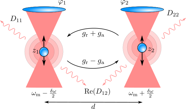
Figure 2: Two nanoparticles are harmonically trapped with frequencies $\omega_{\rm m}\pm\delta\omega/2$ close to the foci of two optical tweezers driven by the same laser with phases $\varphi_{1}$ and $\varphi_{2}$. The light scattered off the particles (i) couples their motion non-reciprocally with coupling rates $g_{\rm r}+g_{\rm a}$ and $g_{\rm r}-g_{\rm a}$, and (ii) imprints photon shot noise, leading to recoil heating with diffusion constants $D_{11}$ and $D_{22}$. The photon shot noise is correlated, as described by Re($D_{12}$).

IV.2 Quantum signatures of optical binding

To expose the core quantum effects of optical binding of linearly interacting particles, we consider the simplest case of two interacting particles of equal volume $V$ and mass $m$, as depicted in Fig. 2 and examined experimentally Rieser et al. (2022).

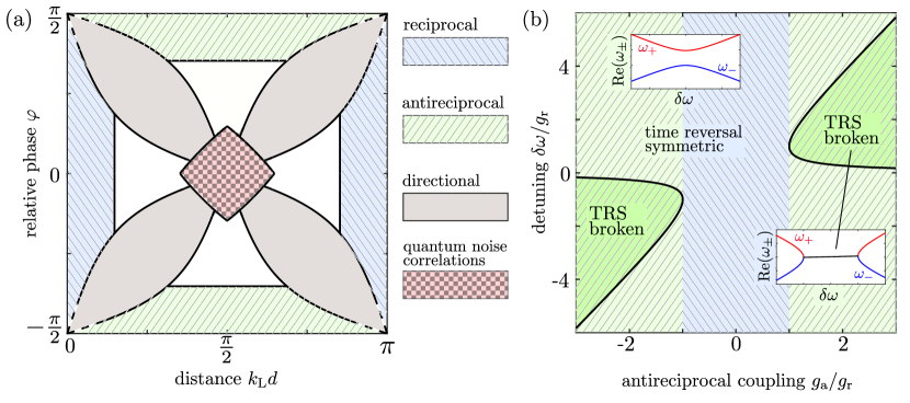
Figure 3: (a) Different regimes of quantum optical binding between two deeply trapped particles as a function of the relative tweezer phase $\varphi$ and the tweezer distance $k_{\rm L}d$. Quantum noise correlations are dominant if $|\text{Re}[2D_{12}/\hbar]|>2\,\text{max}[|C_{12}|,|C_{21}|]$, whereas mainly directional coupling means $|C_{12}|>2|C_{21}|$ or $|C_{21}|>2|C_{12}|$, and reciprocal (antireciprocal) coupling occurs for $|C_{12}+C_{21}|>2|\text{Re}[2D_{12}/\hbar]|$ and $g_{\rm r}>g_{\rm a}$ ($g_{\rm a}>g_{\rm r}$). The dashed lines indicate that the coupling and the quantum noise correlation tend to zero when approaching the corners of the plot, implying that the particles become uncoupled at these points. In the white region none of the effects dominates. (b) Phases of broken and unbroken time reversal symmetry (TRS) as a function of the mechanical detuning $\delta\omega$ and the antireciprocal coupling $g_{\rm a}$. In the blue (green) area the reciprocal coupling is greater (smaller) than the antireciprocal coupling, $g_{\rm r}>g_{\rm a}$ ($g_{\rm a}>g_{\rm r}$). Time reversal symmetry is broken in the dark green region, where the mode frequencies $\text{Re}(\omega_{\pm})$ are degenerate, see insets.

Their corresponding tweezers are located at $\mathbf{d}_{1}=0$ and $\mathbf{d}_{2}=d\mathbf{e}_{y}$ and are linearly polarized, such that

$$\mathbf{E}_{j}=E_{j}e^{i\varphi_{j}}(\cos\Theta_{j}{\bf e}_{x}+\sin\Theta_{j}{\bf e}_{y}),$$ (82)

where $\varphi_{j}$ and $\Theta_{j}$ are the optical phases and their polarization angles, respectively. Defining the tweezer phase difference as $\varphi=\varphi_{1}-\varphi_{2}$, the coupling constants between the two particles take the form

$$C_{12} =C\cos(k_{\rm L}d-\varphi)$$ (83a)

$$C_{21} =C\cos(k_{\rm L}d+\varphi)$$ (83b)

where

$$C=\frac{\varepsilon_{0}\chi^{2}V^{2}k_{\rm L}^{2}(k_{\rm L}-1/z_{\rm R})^{2}}{8\pi d}E_{1}E_{2}\cos\Theta_{1}\cos\Theta_{2}.$$ (84)

The off-diagonal diffusion constants are $D_{12}=\hbar C\sin(k_{\rm L}d)\exp(i\varphi)/2$. The interaction is long-range in nature, which results in a far-field decay of the coupling strength with $1/d$.

These expressions show that the particle dynamics depends strongly on the relative phase and distance between the tweezers. These parameters determine whether the coupling is (i) mostly reciprocal, where Newton’s third law holds approximately, (ii) mostly anti-reciprocal, where action-equals-reaction is violated strongly, (iii) directional, where coupling occurs mainly into one direction, or (iv) whether it is dominated by quantum noise correlations. Fig. 3(a) shows the combination of $\varphi$ and $k_{\rm L}d$ required to reach these coupling regimes.

For completeness, the constant forces are

$$F_{j}= \frac{\varepsilon_{0}\chi^{2}V^{2}k_{\rm L}^{3}(k_{\rm L}-1/z_{\rm R})E_{j}^{2}}{12\pi}$$

$$+\frac{C}{k_{\rm L}-1/z_{\rm R}}\sin(k_{\rm L}d\mp\varphi)$$ (85)

where the upper (lower) sign pertain to $j=1(2)$.

Defining the mean mechanical trapping frequency $\omega_{\rm m}=(\omega_{1}+\omega_{2})/2$ and the intrinsic mechanical frequency difference $\delta\omega=\omega_{2}-\omega_{1}$, the eigenfrequencies $\omega_{\pm}$ of equations (80) can be given explicitly,

$$\omega_{\pm}^{2}= \omega_{\rm m}^{2}+\frac{\delta\omega^{2}}{4}+2\omega_{\rm m}g_{\rm r}$$

$$\pm\omega_{\rm m}\sqrt{\delta\omega^{2}-4\delta\omega g_{\rm a}+4g_{\rm r}^{2}}.$$ (86)

Here we identified the reciprocal and the anti-reciprocal coupling rates

$$g_{\rm r}= g\cos(k_{\rm L}d)\cos\varphi$$ (87a)

$$g_{\rm a}= g\sin(k_{\rm L}d)\sin\varphi$$ (87b)

with $g=C/2m\omega_{\rm m}$, as depicted in Fig. 2.

The quantum Langevin equations (80) are time-reversal symmetric. The system enters a time-reversal-broken phase when the eigenvectors of the coupling matrix in Eq. (80) cannot be chosen real Bender (2007). This is the case for $|g_{\rm a}|>|g_{\rm r}|$ and $|\delta\omega-2g_{\rm a}|<2\sqrt{g_{\rm a}^{2}-g_{\rm r}^{2}}$, see Fig. 3 (b). It turns the squared frequencies $\omega_{\pm}^{2}$ into a complex conjugated pair, implying that one of the two modes grows exponentially in time, while the second one decays. Varying the detuning $\delta\omega$, the system crosses an exceptional point at $\delta\omega=2g_{\rm a}\pm 2\sqrt{g_{\rm a}^{2}-g_{\rm r}^{2}}$. For $|g_{\rm a}|<|g_{\rm r}|$ the system remains in the time-reversal-unbroken phase, for which the squared normal mode frequencies (IV.2) are real.

IV.2.1 Quantum noise in the time-reversal-broken regime

The time-reversal-broken regime can be reached if the anti-reciprocal coupling dominates. We thus maximize the anti-reciprocal coupling and effectively suppress the reciprocal one by setting $\varphi=\pi/2$ and $k_{\rm L}d=2\pi n+\pi/2$ with an integer $n$. The mechanical detuning is chosen as $\delta\omega=2g_{\rm a}$ to maximize the imaginary part of the frequencies (IV.2).

We define the mechanical mode operators by

$$a_{j}=\sqrt{\frac{m\omega_{\rm m}}{2\hbar}}\left(z_{j}+i\frac{p_{j}}{m\omega_{\rm m}}\right),$$ (88)

and transform into the interaction picture by means of $U(t)=\exp[-i\omega_{\rm m}t(a_{1}^{\dagger}a_{1}+a_{2}^{\dagger}a_{2})]$. The recoil heating rate $\gamma_{\rm rec}=D_{11}/\hbar m\omega_{\rm m}$ is approximately the same for both particles for $|\delta\omega|,\gamma_{\rm rec}\ll\omega_{\rm m}$. A rotating wave approximation in the weak-coupling limit $g\ll\omega_{\rm m}$ yields the master equation

$$\partial_{t}\rho\approx \frac{\gamma_{\rm rec}-g}{2}\left[\mathcal{D}[a_{1}+ia_{2}]\rho+\mathcal{D}[a_{1}^{\dagger}-ia_{2}^{\dagger}]\rho\right]$$

$$+\frac{\gamma_{\rm rec}+g}{2}\left[\mathcal{D}[a_{1}^{\dagger}+ia_{2}^{\dagger}]\rho+\mathcal{D}[a_{1}-ia_{2}]\rho\right],$$ (89)

with $\mathcal{D}[A]\cdot=A\cdot A^{\dagger}-\{A^{\dagger}A,\cdot\}/2$.

The master equation (IV.2.1) describes the uncoupled dynamics of the two collective modes $(a_{1}\pm ia_{2})/\sqrt{2}$, which describe motion of the two oscillators at fixed relative phases $\pm\pi/2$. In the absence of quantum noise, the mode $(a_{1}+ia_{2})/\sqrt{2}$ would decay exponentially, while $(a_{1}-ia_{2})/\sqrt{2}$ would increase exponentially. The unavoidable presence of quantum noise due to photon scattering acts as a finite temperature bath, forcing the decaying mode to saturate at the effective occupation $\gamma_{\rm rec}/2g-1/2$. In practice $\gamma_{\rm rec}\gg g$ so that the stationary state of $(a_{1}-ia_{2})/\sqrt{2}$ is typically far away from the ground state, rendering this signature of quantum optical binding relevant for near-future experiments. The alternative choice $\varphi=-\pi/2$ $or$ $k_{\rm L}d=2\pi n-\pi/2$ swaps the roles of $(a_{1}\pm ia_{2})/\sqrt{2}$. Note that in realistic setups, the exponentially increasing mode will eventually approach a stable oscillation amplitude due to the presence of non-linearities in the interaction and unavoidable gas damping.

IV.2.2 Correlated quantum noise

The coupling rates $g_{\rm r}$ and $g_{\rm a}$ can be made to vanish completely by setting $\varphi=0$ and $k_{\rm L}d=2\pi n+\pi/2$. The particles, however, inevitably experience correlated quantum noise, as the cross-diffusion coefficient $D_{12}=D_{21}=\hbar C/2$ is always finite.

Specifically, for equal trapping frequencies, $\delta\omega=0$, the master equation (IV.1.1) reduces to

$$\partial_{t}\rho=-\frac{i}{\hbar}[H_{\rm na},\rho]+\sum_{p=\pm}\frac{2D_{p}}{\hbar^{2}}\mathcal{D}[z_{p}]\rho$$ (90)

with

$$H_{\rm na}=\sum_{j=1}^{2}\frac{p_{j}^{2}}{2m}+\frac{m\omega_{\rm m}^{2}}{2}z_{j}^{2}-F_{j}z_{j},$$ (91)

involving the sum and difference position operators $z_{\pm}=(z_{2}\pm z_{1})/\sqrt{2}$ as well as the diffusion constants $D_{\pm}=\hbar m\omega_{\rm m}(\gamma_{\rm rec}\pm g)$. The center-of-mass and relative position dynamics decouple, but they exhibit different effective recoil rates $\gamma_{\rm rec}\pm g$. In particular, whether the two particles oscillate in phase or in antiphase controls if their scattered fields interfere constructively or destructively, thus locally increasing or decreasing the recoil heating rates. As a consequence, the two modes thermalize to different temperatures in presence of external damping. The resulting temperature difference is proportional to $g/\gamma_{\rm rec}$. It is a direct consequence of the correlation between the quantum noise (and thus cannot be obtained by naively adding single particle recoil heating to the classical equations of motion).

For $k_{\rm L}d=2\pi n-\pi/2$ the two normal modes swap their heating rates, and for $k_{\rm L}d=2\pi n$ and $\varphi=2\pi n\pm\pi/2$ the diffusion rates coincide. This treatment is readily generalized for large particle numbers. In the latter case, a collective mechanical mode may emerge which is characterized by a strongly reduced recoil rate, similar to dark states in superradiant systems Hayn et al. (2011).

IV.2.3 Two-mode-squeezing but no entanglement in free space

One could be tempted to expect that optical binding can induce entanglement between the two particles, given that modulating the relative laser phase in Eq. (IV.1.1) with twice the mechanical frequency, $\varphi=2\omega_{\rm m}t$ yields the two-mode squeezing Hamiltonian

$$H_{\rm na}(t)\approx\frac{\hbar g}{2}\left[a_{-}^{2}+(a_{-}^{\dagger})^{2}\right]$$ (92)

in the interaction picture with respect to $U(t)=\exp[-i\omega_{\rm m}t(a_{1}^{\dagger}a_{1}+a_{2}^{\dagger}a_{2})]$ and after a rotating-wave approximation. Here $a_{-}=(a_{2}-a_{1})/\sqrt{2}$ and we assumed purely conservative interaction $k_{\rm L}d=2\pi n$ and $\delta\omega=0$ for simplicity.

However, far-field optical binding in free space cannot entangle the motion of two particles. This is due to the fact that the master equation (IV.1.1) can be viewed as the ensemble average of a feedback quantum master equation, which models the optical binding interaction between the two particles only via a feed-forward loop of independent and local homodyne measurements.

In this description, the only coherent time evolution is due to the uncoupled oscillator Hamiltonian

$$H_{\rm uc}=\sum_{j=1}^{2}\left(\frac{p_{j}^{2}}{2m_{j}}+\frac{1}{2}\left(m_{j}\omega_{j}^{2}+K_{j}\right)z_{j}^{2}-F_{j}z_{j}\right),$$ (93)

while the interaction between the particles enters incoherently through two processes: First, both particles interact through their coupling to a common bath,

$${\cal D}\rho=\sum_{j,j^{\prime}=1}^{2}\frac{2D_{jj^{\prime}}^{\rm uc}}{\hbar^{2}}\left(z_{j}\rho z_{j^{\prime}}-\frac{1}{2}\{z_{j^{\prime}}z_{j},\rho\}\right),$$ (94)

with the effective diffusion matrix elements

$$D_{11}^{\rm uc}= D_{11}-\frac{\hbar^{2}}{8L_{1}^{2}}-\frac{C_{12}^{2}L_{2}^{2}}{2}$$ (95a)

$$D_{22}^{\rm uc}= D_{22}-\frac{\hbar^{2}}{8L_{2}^{2}}-\frac{C_{21}^{2}L_{1}^{2}}{2},$$ (95b)

and $D_{12}^{\rm uc}=D_{21}^{\rm uc}=\text{Re}(D_{12})$. Here, $L_{j}$ determine the accuracy of homodyning the particle positions Rudolph et al. (2022), which determine the noise strength in the stochastic measurement signal $dy_{j}=\langle z_{j}\rangle dt+L_{j}dW_{j}(t)$ with Wiener increments $dW_{j}(t)$. Second, the two particles are subject to a stochastic homogeneous feedback force described by the superoperator increment

$$d{\cal F}\rho=-\frac{i}{\hbar}\Big{(}C_{12}[z_{1},\rho]\circ dy_{2}(t)+C_{21}[z_{2},\rho]\circ dy_{1}(t)\Big{)},$$ (96)

in Stratonovich calculus. Thus, the measurement signal $dy_{j}$ of particle $j$ determines the force on particle $j^{\prime}\neq j$ and vice versa. Finally, the continuous measurement results in a stochastic localization of the particle state, as described by the superoperator increment Rudolph et al. (2022)

$$d{\cal C}\rho= -\sum_{j=1}^{2}\frac{1}{4L_{j}^{2}}\Big{(}\{z_{j}^{2}-\langle z_{j}^{2}\rangle,\rho\}dt$$

$$+2\{z_{j}-\langle z_{j}\rangle,\rho\}\circ dy_{j}(t)\Big{)}.$$ (97)

In total, the stochastic feedback quantum master equation for the conditional state $\rho_{\rm c}$ reads

$$d\rho_{\rm c}= -\frac{i}{\hbar}[H_{\rm uc},\rho_{\rm c}]dt+{\cal D}\rho_{\rm c}dt+d{\cal F}\rho_{\rm c}+d{\cal C}\rho_{\rm c}.$$ (98)

Converting this to Itô form and taking the ensemble average $\rho=\mathds{E}[\rho_{\rm c}]$ yields the optical binding master equation (III.3).

Note that this equivalence between optical binding and a feed-forward loop requires that the measurement accuracies $L_{j}$ can be chosen such that the diffusion matrix $D_{jj^{\prime}}^{\rm uc}$ is positive. For far-field-coupled particles, where $D_{jj}\gg|D_{12}|,|\hbar C_{jj^{\prime}}|$, this is always possible.

The fact that the feedback quantum master equation (98) exhibits no conservative coupling between the two particles implies that they cannot get entangled. This is in accordance with findings for unidirectional quantum transport Metelmann and Clerk (2017); Clerk (2022) and ultimately a consequence of the fact that the recoil heating rate exceeds the conservative coupling rate between the particles, $\gamma_{\rm rec}>g_{\rm r}$. This constraint can be circumvented in several ways, as discussed next.

IV.2.4 How to entangle through optical binding

In the following, we present three ways to facilitate motional entanglement between the particles through the optical binding interaction, by either reducing $\gamma_{\rm rec}$ or by enhancing $g_{\rm r}$.

Continuous homodyne detection: Photon-induced heating can be reduced by homodyning the position of both particles via detection of the back-scattered light. The thus obtained measurement record may be used to determine the conditional quantum state of the system, which evolves according the optical binding master equation (III.3) together with a stochastic measurement superoperator given in App. D. If the fields are tuned to purely conservative optical-binding interaction, the effective recoil heating rate of the conditional state

$$\gamma_{\rm rec}^{\prime}=\gamma_{\rm rec}(1-\eta_{\rm det}),$$ (99)

is reduced according to the net detection efficiency $\eta_{\rm det}$, as follows from solving the feedback quantum master equation for an infinitesimal time interval. By achieving sufficiently large detection efficiencies, one might thus reduce the recoil heating rate below the conservative coupling rate due to optical binding and thereby enable the generation of entanglement.

Knowledge of the conditional state requires optimal use of all available information, as can be achieved with Kalman filtering Setter et al. (2018); Magrini et al. (2021). In principle, the gained information can also be used for implementing a closed feedback loop by applying an external force conditioned on the measurement record. Controlling the conditional particle state may be used to facilitate entanglement detection Rudolph et al. (2022).

Squeezed vacuum: For small displacements of the particle positions from the tweezer focus, the mechanical momentum of each particle is subject to a single noise quadrature $\xi_{j}$, see Eq. (80). The local recoil rates can be reduced by squeezing the vacuum state in the quadratures commuting with the local noise. In practice, one squeezes a single electromagnetic free-space mode for each particle, ideally with a large overlap $\zeta_{j}$ with the scattered fields of the respective particles. Denoting the squeezing parameters by $r_{j}$ the effective recoil heating rates are given by Gonzalez-Ballestero et al. (2022)

$$\gamma_{{\rm rec},j}^{\prime}=\gamma_{\rm rec}[1-|\zeta_{j}|^{2}(1-e^{-r_{j}})].$$ (100)

Thus, driving the particles with strongly squeezed vacuum modes of large overlap with the scattered fields may suppress the recoil heating rates below the conservative optical-binding interaction, thus facilitating the generation of entanglement.

Note that Eq. (100) is based on tuning the tweezers to a purely conservative optical binding interaction. For finite anti-reciprocal coupling, the particles are subject to noise originating from non-commuting quadratures of the light field, see Eq. (81). This correlation implies that both recoil heating rates cannot be suppressed simultaneously to an arbitrary degree even in the limit of perfect squeezing and full overlap.

Optical cavity: Rather than decreasing the recoil rate, one may enhance the conservative optical-binding interaction by placing the particles in an optical cavity mode $b$ of mode volume $V_{\rm c}$, realizing coherent scattering into the cavity mode Delić et al. (2020); Gonzalez-Ballestero et al. (2019); Windey et al. (2019); Delić et al. (2019). Choosing the tweezer frequency close to the cavity resonance, the cavity field

$$\mathbf{E}_{\rm c}(\mathbf{r})=\sqrt{\frac{2\hbar\omega_{\rm c}}{\varepsilon_{0}V_{c}}}b\,\mathbf{e}_{x}\cos(k_{\rm c}y)$$ (101)

with wavenumber $k_{\rm c}$ and frequency $\omega_{\rm c}=ck_{\rm c}$ adds to the laser field $\mathbf{E}_{\rm L}(\mathbf{r})$ in the optical binding master equation (III.3). Here, we chose the cavity mode to be a standing wave along $y$ and polarized along $x$.

In principle, the presence of the cavity mirrors modifies the electromagnetic Green tensor in Eq. (III.3) as well as the scattering modes appearing in (68). However, these modifications can be neglected for typical macroscopic cavities, so that the cavity enters solely through providing the additional mode $b$. Note that light scattering into this cavity mode is enhanced by the Purcell effect, rendering cavity-mediated interactions dominant in comparison to coupling via the free-space modes. Since the cavity output can be detected with high efficiency, such a setup may be utilized for entanglement via single-photon detection and post-selection Rudolph et al. (2020).

IV.2.5 Unidirectional quantum transport

The optical binding interaction between two particles can be chosen unidirectional for $g_{\rm r}=\pm g_{\rm a}$, such that one particle influences the other but not vice versa. For instance, this can be achieved by setting $k_{\rm L}d\mp\varphi=\pi n+\pi/2$, so that the scattering fields interfere destructively in one direction and constructively in the opposite one. Maximizing the unidirectional coupling in direction of particle $j=1$ with $\varphi=k_{\rm L}d=2\pi n+\pi/4$, the coupling constants take the form $C_{12}=C$, $C_{21}=0$, while the cross diffusion coefficient reduces to $D_{12}=\hbar C(1+i)/4$. The master equation (IV.1.1) then becomes

$$\partial_{t}\rho= -\frac{i}{\hbar}[H_{\rm uc},\rho]+\sum_{j,j^{\prime}=1}^{2}\frac{2D_{jj^{\prime}}^{\rm uni}}{\hbar^{2}}\left(z_{j}\rho z_{j^{\prime}}-\frac{1}{2}\{z_{j}z_{j^{\prime}},\rho\}\right)$$

$$+\frac{C}{2\hbar}\Bigl{[}i[z_{1},\{z_{2},\rho\}]+\mathcal{D}[z_{1}]\rho+\mathcal{D}[z_{2}]\rho\Bigr{]},$$ (102)

with the real-valued diffusion constants $D_{12}^{\rm uni}=D_{21}^{\rm uni}=\hbar C/4$ and $D_{jj}^{\rm uni}=D_{jj}-D_{12}^{\rm uni}$.

The master equation (IV.2.5) decomposes into two parts: (i) The first line describes unitary and uncoupled dynamics of the two particles through the Hamiltonian $H_{\rm uc}$ as well as correlated quantum noise on the two particles. (ii) The second line features the standard form of unidirectional transport between quantum systems Metelmann and Clerk (2017); Clerk (2022). Unidirectionality can serve as technological resource, such as for non-hermitian quantum sensing Lau and Clerk (2018); McDonald and Clerk (2020) or for directional amplification in chains of multiple oscillators Wanjura et al. (2020, 2021).

In arrays of $N>2$ particles one must account for the fact that the optical binding interaction is long-range and proportional to $1/d_{jj^{\prime}}$, see Eq. (IV.1.1). In general, the dynamics are thus not described by nearest-neighbor couplings. A few important consequences are:

1. It is impossible to build a unidirectional chain, where the transport of excitations takes place in one direction only. Instead, choosing the nearest neighbor tweezer phase difference as $\pi/4$ and the nearest neighbor distances as $(2\pi n+\pi/4)/k_{\rm L}$ with $n\in\mathbb{N}$, the coupling constants are always positive in one direction while alternating in sign in the other direction. Directional amplification might still be possible in such chains, which may enable signal enhancement in arrays of nanoparticles Lau and Clerk (2018).

2. The long-range physical arrangement of the particles matters because even distant particles influence each other. For instance, a circle of particles is in general not describable by a one-dimensional chain with periodic boundary conditions.

3. Paradigmatic phenomena of non-hermiticity in particle arrays, such as the non-hermitian skin effect Yao and Wang (2018); Bergholtz et al. (2021), may be altered given that the edges of the particle array may still interact directly. In fact, the concept of edges is no longer fully applicable in the presence of long-range interactions, with potentially far-reaching consequences for the non-hermitian bulk-boundary correspondence Bergholtz et al. (2021).

V Outlook

We conclude this article by outlining some possible generalizations of the theory presented.

Rotational optical binding.– The master equation (III.3) describes light-induced torques between co-levitated nanoparticles due to their anisotropic susceptibility tensors. While the results of Sec. IV are readily adapted to the libration regime of strongly aligned particles, they must be generalized whenever the inherent non-linearity of rotations starts to contribute strongly Stickler et al. (2021). Answering questions such as if rotational entanglement can be realized through optical binding requires understanding the quantum dynamics of co-rotating particles in presence of reciprocal and non-reciprocal interactions. The analysis will have to account for both the full non-linearity of rotations as well as for the possible coupling between the particle rotation and center-of-mass motion.

Non-linear optical binding.– Our discussion of quantum optical binding in Sec. IV assumes that the optical binding interaction may be linearized in the particle positions. In the absence of strong cooling this approximation will fail eventually if time-reversal symmetry is broken, since the particle amplitudes increase exponentially with time and non-linearities of both the trapping potential and the optical-binding interaction become relevant. The two-particle dynamics may then exhibit multi-stability and stable limit cycles, with great potential for sensing Strogatz (2018). The properties of these limit cycles in the quantum regime and their relation to continuous time crystals Kongkhambut et al. (2022) are open questions.

Near-field optical binding.– A second core assumption in Sec. IV is that the distance between the particles is sufficiently large, so that only the far-field contribution to light scattering is relevant. While this is well justified in state-of-the-art setups, near-field optical binding may well become relevant in future experiments if the distances between particles become comparable to the laser wavelength. Investigating light-induced coupling in the near-field requires taking into account that the laser fields levitating two particles at close distances overlap significantly. Whether the tunability of optical binding can be retained in such a situation is still unclear, as is whether the impossibility of generating entanglement via optical binding carries over to the near field. Naively evaluating the near-field coupling strength would suggest that entanglement can indeed be generated, but this argument fails for commonly used nanoparticles because approximating the scattered fields as homogeneous across neighboring particles cannot be justified at close distances.

Large particles.– Our theory assumes the size of the dielectric particles to be small in comparison to the wavelengths of the incoming light fields and the distance between neighboring particles. This approximation allows for deriving the Lagrangian in Sec. II which yields the correct conservative light-matter interaction. Generalizing this treatment to situations where the wavelength becomes comparable or even greater than the particle size, where internal Mie resonances Maurer et al. (2021, 2022) and multiple scattering events become relevant Karásek et al. (2008), is a prerequisite to study quantum optical binding between large objects.

Optical binding in microcavities.– Microcavities yield strong coupling to nanoparticles Wachter et al. (2019) due to their small mode volume, rendering them attractive for interfacing levitated nanoparticles via optical binding. Adapting the optical binding master equation (III.3) to this situation requires the correct electromagnetic field modes (or, equivalently, the Green tensor) for such a highly confined geometry. This will change the master equation in two ways: (i) the conservative interaction is determined by the adapted Green tensor; (ii) when tracing out the vacuum field, the proper modes must be used rather than the free-space ones to avoid mode overcounting, yielding modified Lindblad operators.

In summary, we presented the quantum theory of light-induced interactions in arrays of levitated nanoparticles, and used it to identify unique signatures of quantum optical binding which may be observed in state-of-the-art experiments. We expect that the ability to continuously tune the interaction from fully reciprocal to fully non-reciprocal will render nanoparticle arrays an ideal platform for exploring and exploiting non-hermitian quantum physics.

Appendix A Lorentz force and torque on a polarized object

This section derives the total force and torque acting on a particle polarized with internal polarization field $\mathbf{P}(\mathbf{r})$ in presence of the electric field $\mathbf{E}(\mathbf{r})$ and magnetic field $\mathbf{B}(\mathbf{r})$, as used in Eq. (9). The associated polarization charge and current densities are $\rho_{\rm P}(\mathbf{r})=-\nabla\cdot\mathbf{P}(\mathbf{r})$ and $\mathbf{j}_{\rm P}(\mathbf{r})=\partial_{t}\mathbf{P}(\mathbf{r})$, respectively.

The total force $\mathbf{F}$ acting on the particle is obtained by integrating the Lorentz force density Barnett and Loudon (2006); Novotny and Hecht (2012)

$$\mathbf{f}_{\rm L}(\mathbf{r})=-[\nabla\cdot\mathbf{P}(\mathbf{r})]\mathbf{E}(\mathbf{r})+\partial_{t}\mathbf{P}(\mathbf{r})\times\mathbf{B}(\mathbf{r})$$ (103)

over the particle volume $\mathcal{V}$. Integration by parts yields

$$\mathbf{F}=\int_{\mathcal{V}}d^{3}\mathbf{r}\Big{[}[\mathbf{P}(\mathbf{r})\cdot\nabla]\mathbf{E}(\mathbf{r})+\partial_{t}\mathbf{P}(\mathbf{r})\times\mathbf{B}(\mathbf{r})\Big{]},$$ (104)

which can be rewritten as

$$\mathbf{F}=\int_{\mathcal{V}}d^{3}\mathbf{r}\Big{[}\nabla^{\prime}[\mathbf{P}(\mathbf{r})\cdot\mathbf{E}(\mathbf{r}^{\prime})]_{\mathbf{r}^{\prime}=\mathbf{r}}+\partial_{t}[\mathbf{P}(\mathbf{r})\times\mathbf{B}(\mathbf{r})]\Big{]},$$ (105)

where we used Faraday’s law $\nabla\times\mathbf{E}(\mathbf{r})=-\partial_{t}\mathbf{B}(\mathbf{r})$ and $\nabla[\mathbf{a}\cdot\mathbf{E}(\mathbf{r})]=(\mathbf{a}\cdot\nabla)\mathbf{E}(\mathbf{r})+\mathbf{a}\times[\nabla\times\mathbf{E}(\mathbf{r})]$ for a constant vector $\mathbf{a}$. For rapidly oscillating fields, such as for dielectric particles in optical fields, the time derivative averages to zero so that only Eq. (9a) remains Barnett and Loudon (2006); Novotny and Hecht (2012).

The total torque $\mathbf{N}$ can be obtained by integrating the Lorentz torque density $\mathbf{r}\times\mathbf{f}_{\rm L}(\mathbf{r})$ over the particle volume. Partial integration shows that the total torque Barnett and Loudon (2006)

$$\mathbf{N}=\int_{\mathcal{V}}d^{3}\mathbf{r}\bigg{[}\mathbf{P}(\mathbf{r})\times\mathbf{E}(\mathbf{r})+\mathbf{r}\times\Big{[}[\mathbf{P}(\mathbf{r})\cdot\nabla]\mathbf{E}(\mathbf{r})+\partial_{t}\mathbf{P}(\mathbf{r})\times\mathbf{B}(\mathbf{r})\Big{]}\bigg{]},$$ (106)

contains two contributions: (i) The first term describes the intrinsic torque on each volume element; (ii) the second term is the orbital torque density resulting from the effective local force density in Eq. (104). Using Faraday’s law, the above vector identity, and averaging the time derivative to zero, one obtains

$$\mathbf{N}=\int_{\mathcal{V}}d^{3}\mathbf{r}\bigg{[}\mathbf{P}(\mathbf{r})\times\mathbf{E}(\mathbf{r})+\mathbf{r}\times\Big{[}\nabla^{\prime}[\mathbf{P}(\mathbf{r})\cdot\mathbf{E}(\mathbf{r}^{\prime})]_{\mathbf{r}^{\prime}=\mathbf{r}}\Big{]}\bigg{]}.$$ (107)

Subtracting the orbital torque $\mathbf{r}_{\rm cm}\times\mathbf{F}$ acting on the particle center of mass $\mathbf{r}_{\rm cm}$ yields the torque (9).

Appendix B Approximating the total Lagrange function

This appendix describes the approximations that lead from Eq. (10) to Eq. (31). Explicitly, Eqs. (23), (28) and (29) are inserted into Eq. (10). Using that the external field $\mathbf{A}_{\rm ext}(\mathbf{r},t)$ varies little over the volume of each particle yields

$$L_{\rm tot}\approx L_{\rm m}+L_{\rm em}-V_{\rm ext}+\varepsilon_{0}\sum_{j=1}^{N}\int_{\mathcal{V}_{j}}d^{3}\mathbf{r}\left(\frac{1}{2}\partial_{t}\mathbf{A}(\mathbf{r})\cdot\upchi_{j}\partial_{t}\mathbf{A}(\mathbf{r})+\partial_{t}\mathbf{A}(\mathbf{r})\cdot\upchi_{j}\partial_{t}\mathbf{A}_{\rm ext}(\mathbf{r},t)\right)$$

$$+\varepsilon_{0}\sum_{\begin{subarray}{c}j,j^{\prime}=1\\ j\neq j^{\prime}\end{subarray}}^{N}\int_{\mathcal{V}_{j}}d^{3}\mathbf{r}\int_{\mathcal{V}_{j^{\prime}}}d^{3}\mathbf{r}^{\prime}\left(\frac{1}{2}\partial_{t}\mathbf{A}(\mathbf{r})\cdot\upchi_{j}{\sf G}_{0}(\mathbf{r}-\mathbf{r}^{\prime})\upchi_{j^{\prime}}\partial_{t}\mathbf{A}(\mathbf{r}^{\prime})+\partial_{t}\mathbf{A}(\mathbf{r})\cdot\upchi_{j}{\sf G}_{0}(\mathbf{r}-\mathbf{r}^{\prime})\upchi_{j^{\prime}}\partial_{t}\mathbf{A}_{\rm ext}(\mathbf{r}^{\prime},t)\right)$$ (108)

$$+\int d^{3}\mathbf{r}\left(\frac{\varepsilon_{0}}{2}[\partial_{t}\mathbf{A}_{\rm ext}(\mathbf{r},t)]^{2}-\frac{1}{2\mu_{0}}[\nabla\times\mathbf{A}_{\rm ext}(\mathbf{r},t)]^{2}+\varepsilon_{0}\partial_{t}\mathbf{A}_{\rm ext}(\mathbf{r},t)\cdot\partial_{t}\mathbf{A}(\mathbf{r})-\frac{1}{\mu_{0}}[\nabla\times\mathbf{A}_{\rm ext}(\mathbf{r},t)]\cdot[\nabla\times\mathbf{A}(\mathbf{r})]\right)$$

Here, $V_{\rm ext}$ collects those terms in which the external field $\mathbf{A}_{\rm ext}(\mathbf{r})$ is integrated over the particle volume only.

We can neglect the light-matter interaction terms that are quadratic in the scattering fields $\mathbf{A}(\mathbf{r})$ since the latter are a small perturbation to the external laser field. In addition, the second term in the second line is negligible when compared to the last term of the first line, which both describe interaction between the external field and the scattering field, since the susceptibility is proportional to the particle volume. The last line of Eq. (B) can be simplified by performing a partial integration shifting the curls to $\mathbf{A}_{\rm ext}(\mathbf{r},t)$, which is transverse and fulfills the homogeneous wave equation (30). Altogether,

$$L_{\rm tot}\approx L_{\rm m}+L_{\rm em}-V_{\rm ext}-\varepsilon_{0}\sum_{j=1}^{N}\int_{\mathcal{V}_{j}}d^{3}\mathbf{r}\Big{[}\mathbf{E}_{\rm ext}(\mathbf{r},t)\cdot\upchi_{j}\partial_{t}\mathbf{A}(\mathbf{r})\Big{]}-\varepsilon_{0}\frac{d}{dt}\int d^{3}\mathbf{r}\left[\left(\frac{1}{2}\mathbf{A}_{\rm ext}(\mathbf{r},t)+\mathbf{A}(\mathbf{r})\right)\cdot\mathbf{E}_{\rm ext}(\mathbf{r},t)\right].$$ (109)

The last term can be gauged away, such that by defining the mechanical gauge function Craig and Thirunamachandran (1998)

$$S=\varepsilon_{0}\sum_{j=1}^{N}\int_{\mathcal{V}_{j}}d^{3}\mathbf{r}\left[\mathbf{E}_{\rm ext}(\mathbf{r},t)\cdot\upchi_{j}\mathbf{A}(\mathbf{r})\right]+\varepsilon_{0}\int d^{3}\mathbf{r}\left[\left(\frac{1}{2}\mathbf{A}_{\rm ext}(\mathbf{r},t)+\mathbf{A}(\mathbf{r})\right)\cdot\mathbf{E}_{\rm ext}(\mathbf{r},t)\right],$$ (110)

the Lagrangian takes the form

$$L_{\rm tot}=L_{\rm m}+L_{\rm em}-V_{\rm ext}-V_{\rm int}-\frac{dS}{dt}+\varepsilon_{0}\sum_{j=1}^{N}\sum_{q_{j}}\dot{q}_{j}\frac{\partial}{\partial q_{j}}\int_{\mathcal{V}_{j}}d^{3}\mathbf{r}\left[\mathbf{E}_{\rm ext}(\mathbf{r},t)\cdot\upchi_{j}\mathbf{A}(\mathbf{r})\right].$$ (111)

If the particles move much slower than the external light field changes, the last term can be neglected and one arrives at $L_{\rm tot}\approx L-dS/dt$ as used in the main text.

Appendix C Quantum Langevin equations

This Appendix derives the optical binding quantum Langevin equations which are equivalent to the master equation (III.3). They are required to obtain the linearized Langevin equations (80).

Our starting point is the Heisenberg equations of motion resulting from the total light-matter Hamiltonian (36),

$$\dot{q}_{j}= \frac{\partial}{\partial p_{j}}H_{\rm m}$$ (112a)

$$\dot{p}_{j}= -\frac{\partial}{\partial q_{j}}(H_{\rm m}+V_{\rm ext}+V_{\rm int}).$$ (112b)

They depend on the optical degrees of freedom through the interaction potential $V_{\rm int}$. The Heisenberg equations for the light fields,

$$\dot{b}_{\mathbf{k}s}=-i\omega_{k}b_{\mathbf{k}s}+\frac{\varepsilon_{0}\omega_{\rm L}}{\sqrt{8\hbar\omega_{k}\varepsilon_{0}L^{3}}}\sum_{j=1}^{N}\int_{\mathcal{V}_{j}}d^{3}\mathbf{r}e^{-i\mathbf{k}\cdot\mathbf{r}}\mathbf{t}_{\mathbf{k}s}^{*}\cdot\upchi_{j}[\mathbf{E}_{\rm L}(\mathbf{r})e^{-i\omega_{\rm L}t}-\text{c.c.}],$$ (113)

can be solved as function of the coordinate operators,

$$b_{\mathbf{k}s}(t)=b_{\mathbf{k}s}(t_{0})e^{-i\omega_{k}(t-t_{0})}+\frac{\varepsilon_{0}\omega_{\rm L}}{\sqrt{8\hbar\omega_{k}\varepsilon_{0}L^{3}}}\sum_{j=1}^{N}\int_{t_{0}}^{t}dt^{\prime}\int_{\mathcal{V}_{j}(t^{\prime})}d^{3}\mathbf{r}e^{-i\mathbf{k}\cdot\mathbf{r}}\mathbf{t}_{\mathbf{k}s}^{*}\cdot\upchi_{j}(t^{\prime})[\mathbf{E}_{\rm L}(\mathbf{r})e^{-i\omega_{\rm L}t^{\prime}}-\text{c.c.}].$$ (114)

Inserting this into Eq. (112) yields a closed system of Heisenberg equations for the mechanical degrees of freedom.

We now divide the time axis into intervals of width $\Delta t$ much greater than a single optical period $1/\omega_{\rm L}$, but much smaller than the timescale of mechanical motion. Integrating the momentum equations of motion over one time step, the momentum change $\Delta p_{j}(t)=p_{j}(t+\Delta t)-p_{j}(t)$ is given by

$$\Delta p_{j}(t)\approx -\frac{\partial}{\partial q_{j}}(H_{\rm m}+\bar{V}_{\rm ext})\Delta t+\xi_{q}^{j}\Delta t$$

$$+\Bigg{[}\frac{\partial}{\partial q_{j}}\int_{t}^{t+\Delta t}dt^{\prime}\int_{t}^{t^{\prime}}dt^{\prime\prime}\sum_{\mathbf{k}s}\int_{\mathcal{V}_{j}(t^{\prime})}d^{3}\mathbf{r}\int_{\mathcal{V}_{j^{\prime}}(t^{\prime\prime})}d^{3}\mathbf{r}^{\prime}\frac{\omega_{\rm L}^{2}\varepsilon_{0}}{8i\omega_{k}L^{3}}$$

$$\times\Big{[}e^{i\mathbf{k}\cdot(\mathbf{r}-\mathbf{r}^{\prime})}e^{-i\omega_{k}(t^{\prime}-t^{\prime\prime})}\mathbf{t}_{\mathbf{k}s}\cdot\upchi_{j}(t^{\prime})[\mathbf{E}_{\rm L}(\mathbf{r})e^{-i\omega_{\rm L}t^{\prime}}-\text{c.c.}]\mathbf{t}_{\mathbf{k}s}^{*}\cdot\upchi_{j^{\prime}}(t^{\prime\prime})[\mathbf{E}_{\rm L}(\mathbf{r^{\prime}})e^{-i\omega_{\rm L}t^{\prime\prime}}-\text{c.c.}]-\text{h.c.}\Big{]}\Bigg{]}_{j^{\prime}=j}$$

$$+\frac{\partial}{\partial q_{j}}\sum_{\begin{subarray}{c}j^{\prime}=1\\ j^{\prime}\neq j\end{subarray}}^{N}\int_{t}^{t+\Delta t}dt^{\prime}\int_{t}^{t^{\prime}}dt^{\prime\prime}\sum_{\mathbf{k}s}\int_{\mathcal{V}_{j}(t^{\prime})}d^{3}\mathbf{r}\int_{\mathcal{V}_{j^{\prime}}(t^{\prime\prime})}d^{3}\mathbf{r}^{\prime}\frac{\omega_{\rm L}^{2}\varepsilon_{0}}{8i\omega_{k}L^{3}}$$

$$\times\Big{[}e^{i\mathbf{k}\cdot(\mathbf{r}-\mathbf{r}^{\prime})}e^{-i\omega_{k}(t^{\prime}-t^{\prime\prime})}\mathbf{t}_{\mathbf{k}s}\cdot\upchi_{j}(t^{\prime})[\mathbf{E}_{\rm L}(\mathbf{r})e^{-i\omega_{\rm L}t^{\prime}}-\text{c.c.}]\mathbf{t}_{\mathbf{k}s}^{*}\cdot\upchi_{j^{\prime}}(t^{\prime\prime})[\mathbf{E}_{\rm L}(\mathbf{r^{\prime}})e^{-i\omega_{\rm L}t^{\prime\prime}}-\text{c.c.}]-\text{h.c.}\Big{]},$$ (115)

where $\bar{V}_{\rm ext}$ is the time-averaged external potential $V_{\rm ext}$. The radiation pressure shot noise operators

$$\xi_{q}^{j}\Delta t=\frac{\partial}{\partial q_{j}}\int_{t}^{t+\Delta t}dt^{\prime}\sum_{\mathbf{k}s}\int_{\mathcal{V}_{j}(t^{\prime})}d^{3}\mathbf{r}\frac{\omega_{\rm L}}{2i}\sqrt{\frac{\hbar\varepsilon_{0}}{2\omega_{k}L^{3}}}\left[\mathbf{t}_{\mathbf{k}s}e^{i\mathbf{k}\cdot\mathbf{r}}e^{-i\omega_{k}(t^{\prime}-t)}b_{\mathbf{k}s}(t)+\text{h.c.}\right]\cdot\upchi_{j}(t^{\prime})[\mathbf{E}_{\rm L}(\mathbf{r})e^{-i\omega_{\rm L}t^{\prime}}-\text{c.c.}]$$ (116)

describe the generalized forces due to the light-matter interaction when ignoring the backaction of the scattered light on the particles. The term in the second and third line describes the effect of radiation pressure on the $j$th particle, while the fourth and fifth line describes the scattering contribution to the optical binding interaction between particles $j$ and $j^{\prime}$.

We now perform the Markov approximation by replacing all coordinate operators as $q_{j}(t^{\prime})\simeq q_{j}(t)$. Then we evaluate all integrals over $t^{\prime}$ and $t^{\prime\prime}$ by using the relations in Sec. III, such as $\pi\delta(\omega_{\rm L}-\omega_{k})+i\mathcal{P}[1/(\omega_{\rm L}-\omega_{k})]=1/i(\omega_{k}-\omega_{\rm L}-i\eta)$. Utilizing Eq. (54), one can rewrite the following integral as

$$\int_{\mathcal{V}_{j}}d^{3}\mathbf{r}\int_{\mathcal{V}_{j^{\prime}}}d^{3}\mathbf{r}^{\prime}\int d^{3}\mathbf{k}\sum_{s}\frac{k_{\rm L}^{2}\varepsilon_{0}\Delta t}{4(2\pi)^{3}}\left[e^{i\mathbf{k}\cdot(\mathbf{r}-\mathbf{r}^{\prime})}\mathbf{t}_{\mathbf{k}s}\cdot\upchi_{j}\mathbf{E}_{\rm L}^{*}(\mathbf{r})\frac{1}{k^{2}-k_{\rm L}^{2}-i\eta}\mathbf{t}_{\mathbf{k}s}^{*}\cdot\upchi_{j^{\prime}}\mathbf{E}_{\rm L}(\mathbf{r}^{\prime})+\text{h.c.}\right]$$

$$=\int_{\mathcal{V}_{j}}d^{3}\mathbf{r}\int_{\mathcal{V}_{j^{\prime}}}d^{3}\mathbf{r}^{\prime}\frac{\varepsilon_{0}\Delta t}{4}\Big{[}\mathbf{E}_{\rm L}^{*}(\mathbf{r})\cdot\upchi_{j}[{\sf G}(\mathbf{r}-\mathbf{r^{\prime}})-{\sf G}_{0}(\mathbf{r}-\mathbf{r^{\prime}})]\upchi_{j^{\prime}}\mathbf{E}_{\rm L}(\mathbf{r})+\text{h.c.}\Big{]}.$$ (117)

For $j^{\prime}\neq j$ the volume integrals can be replaced by the respective total volume, and for $j^{\prime}=j$ Eq. (59) holds.

The shot noise force operators (116) are not necessarily Gaussian. Its first and second moments are

$$\langle\xi_{q}^{j}(t)A_{\rm mec}\rangle =0$$ (118a)

$$\langle\xi_{q^{\prime}}^{j^{\prime}}(t^{\prime})A_{\rm mec}\xi_{q}^{j}(t)B_{\rm mec}\rangle =\int d^{3}\mathbf{k}\sum_{s}\frac{\hbar\varepsilon_{0}\omega_{\rm L}^{2}}{8\omega_{k}(2\pi)^{3}}\text{sinc}^{2}\left(\frac{\omega_{\rm L}-\omega_{k}}{2}\Delta t\right)e^{-i(\omega_{k}-\omega_{\rm L})(t^{\prime}-t)}$$

$$\times\Bigg{\langle}\left[\frac{\partial}{\partial q^{\prime}_{j^{\prime}}}\int_{\mathcal{V}_{j^{\prime}}}d^{3}\mathbf{r}^{\prime}\,\mathbf{t}_{\mathbf{k}s}\cdot\upchi_{j^{\prime}}\mathbf{E}_{\rm L}^{*}(\mathbf{r}^{\prime})e^{i\mathbf{k}\cdot\mathbf{r}^{\prime}}\right]A_{\rm mec}\left[\frac{\partial}{\partial q_{j}}\int_{\mathcal{V}_{j}}d^{3}\mathbf{r}\,\mathbf{t}_{\mathbf{k}s}^{*}\cdot\upchi_{j}\mathbf{E}_{\rm L}(\mathbf{r})e^{-i\mathbf{k}\cdot\mathbf{r}}\right]B_{\rm mec}\Bigg{\rangle},$$ (118b)

for arbitrary operator $A_{\rm mec}$ and $B_{\rm mec}$ acting in the mechanical Hilbert space. Here, we took the electromagnetic field to be in the vacuum at $t$.

We now use that for functions $f(\omega_{k})$ varying slowly in relation to $1/\Delta t$,

$$\int_{0}^{\infty}d\omega_{k}\,f(\omega_{k})\text{sinc}^{2}\left(\frac{\omega_{\rm L}-\omega_{k}}{2}\Delta t\right)e^{-i(\omega_{k}-\omega_{\rm L})\tau}\approx f(\omega_{\rm L})\int_{0}^{\infty}d\omega_{k}\,\text{sinc}^{2}\left(\frac{\omega_{\rm L}-\omega_{k}}{2}\Delta t\right)e^{-i(\omega_{k}-\omega_{\rm L})\tau}\approx 2\pi f(\omega_{\rm L})\delta(\tau),$$ (119)

to get

$$\langle\xi_{q^{\prime}}^{j^{\prime}}(t^{\prime})A_{\rm mec}\xi_{q}^{j}(t)B_{\rm mec}\rangle= \int d^{2}\mathbf{n}\sum_{s}\frac{\hbar\varepsilon_{0}k_{\rm L}^{3}}{32\pi^{2}}\delta(t-t^{\prime})$$

$$\times\left\langle\left[\frac{\partial}{\partial q^{\prime}_{j^{\prime}}}V_{j^{\prime}}\mathbf{t}_{\mathbf{n}s}\cdot\upchi_{j^{\prime}}\mathbf{E}_{\rm L}^{*}(\mathbf{r}_{j^{\prime}})e^{ik_{\rm L}\mathbf{n}\cdot\mathbf{r}_{j^{\prime}}}\right]A_{\rm mec}\left[\frac{\partial}{\partial q_{j}}V_{j}\mathbf{t}_{\mathbf{n}s}^{*}\cdot\upchi_{j}\mathbf{E}_{\rm L}(\mathbf{r}_{j})e^{-ik_{\rm L}\mathbf{n}\cdot\mathbf{r}_{j}}\right]B_{\rm mec}\right\rangle.$$ (120)

In the limit of small time steps, Eqs. (C) turn into the quantum Langevin equations of optical binding,

$$\dot{q}_{j}= \frac{\partial}{\partial p_{j}}H_{\rm m}$$ (121a)

$$\dot{p}_{j}= -\frac{\partial}{\partial q_{j}}(H_{\rm m}+V_{\rm L})+\frac{\varepsilon_{0}k_{\rm L}^{3}V_{j}}{12\pi}\text{Im}\left[\mathbf{E}_{\rm L}^{*}(\mathbf{r}_{j})\cdot\upchi_{j}\frac{\partial}{\partial q_{j}}V_{j}\upchi_{j}\mathbf{E}_{\rm L}(\mathbf{r}_{j})\right]$$

$$+\frac{\partial}{\partial q_{j}}\sum_{\begin{subarray}{c}j^{\prime}=1\\ j^{\prime}\neq j\end{subarray}}^{N}\frac{\varepsilon_{0}V_{j}V_{j^{\prime}}}{2}\text{Re}\left[\mathbf{E}_{\rm L}^{*}(\mathbf{r}_{j})\cdot\upchi_{j}{\sf G}(\mathbf{r}_{j}-\mathbf{r}_{j^{\prime}})\upchi_{j^{\prime}}\mathbf{E}_{\rm L}(\mathbf{r}_{j^{\prime}})\right]+\xi_{q}^{j}.$$ (121b)

The expectation value of these equations yields the averaged classical optical binding equations of motion, whose center-of-mass version was derived in Dholakia and Zemánek (2010); Rieser et al. (2022). The same equations are obtained from the Ehrenfest equations resulting from the optical binding master equation (III.3). This confirms the equivalence between the optical binding master equation (III.3) and the quantum Langevin equations (121).

The noise operators in (121) are characterized by their first and second moments (118) and (C) as well as all higher moments following from the definition (116). In the regime of linear harmonic motion, the first two moments suffice to characterize the noise, which is thus Gaussian. In order to calculate its correlator, one requires the second moments with $A_{\rm mec}=\mathbb{1}$. In this case, the integral over all scattering directions $\mathbf{n}$ can be evaluated explicitly, so that for $j\neq j^{\prime}$,

$$\langle\xi_{q^{\prime}}^{j^{\prime}}(t^{\prime})\xi_{q}^{j}(t)B_{\rm mec}\rangle=\frac{\hbar\varepsilon_{0}}{8}\delta(t-t^{\prime})\left\langle\frac{\partial^{2}}{\partial q^{\prime}_{j^{\prime}}\partial q_{j}}V_{j}V_{j^{\prime}}\mathbf{E}_{\rm L}^{*}(\mathbf{r}_{j^{\prime}})\cdot\upchi_{j^{\prime}}\text{Im}[{\sf G}(\mathbf{r}_{j}-\mathbf{r}_{j^{\prime}})]\upchi_{j}\mathbf{E}_{\rm L}(\mathbf{r}_{j})B_{\rm mec}\right\rangle,$$ (122)

while for $j=j^{\prime}$,

$$\langle\xi_{q^{\prime}}^{j}(t^{\prime})\xi_{q}^{j}(t)B_{\rm mec}\rangle= \frac{\hbar\varepsilon_{0}k_{\rm L}^{3}}{60\pi}\delta(t-t^{\prime})\Bigg{\langle}\Bigg{[}5\bigg{[}\frac{\partial}{\partial q^{\prime}_{j}}V_{j}\upchi_{j}\mathbf{E}_{\rm L}^{*}(\mathbf{r}_{j})\bigg{]}\cdot\bigg{[}\frac{\partial}{\partial q_{j}}V_{j}\upchi_{j}\mathbf{E}_{\rm L}(\mathbf{r}_{j})\bigg{]}+2k_{\rm L}^{2}\frac{\partial\mathbf{r}_{j}}{\partial q^{\prime}_{j}}\cdot\frac{\partial\mathbf{r}_{j}}{\partial q_{j}}|V_{j}\upchi_{j}\mathbf{E}_{\rm L}(\mathbf{r}_{j})|^{2}$$

$$-k_{\rm L}^{2}\bigg{[}V_{j}\frac{\partial\mathbf{r}_{j}}{\partial q^{\prime}_{j}}\cdot\upchi_{j}\mathbf{E}_{\rm L}^{*}(\mathbf{r}_{j})\bigg{]}\bigg{[}V_{j}\frac{\partial\mathbf{r}_{j}}{\partial q_{j}}\mathbf{r}_{j}\cdot\upchi_{j}\mathbf{E}_{\rm L}(\mathbf{r}_{j})\bigg{]}\Bigg{]}B_{\rm mec}\Bigg{\rangle}.$$ (123)

For $B_{\rm mec}=\mathbb{1}$ and for $q=q^{\prime}$ given by the equilibrium coordinates in an optical tweezer, this last expression reduces to the recoil diffusion rates of small ellipsoidal rotors Schäfer et al. (2021).

To get the linearized Langevin equations (80) between small spheres, Eqs. (121) must be expanded harmonically around the tweezer foci following the same steps as in Sec. IV.1 and renaming $\xi_{j}=\xi_{z}^{j}$. The corresponding correlators (81) are obtained by evaluating Eqs. (122) and (C) at the tweezer foci.

Appendix D Recoil noise reduction via homodyne detection

This appendix explains why continuous homodyning effectively reduces the recoil heating rate, as stated in Sec. IV.2.4. We start by considering a single particle, the generalization to two particles is straightforward and will be discussed afterwards.

Homodyning the scattered field with net detection efficiency of $\eta_{\rm det}$ and local-oscillator phase $\phi$ measures the particle position $z$ with signal $dy(t)=\langle z\rangle\cos\phi\,dt+\hbar\,dW(t)/\sqrt{8D\eta_{\rm det}}$, where $D$ is the recoil diffusion constant (79) and $dW(t)$ is a Wiener increment. The measurement backaction enters the dynamics of the conditional state $\rho_{\rm c}$ through a stochastic term in the quantum master equation in Itô form Rudolph et al. (2022)

$$d\rho_{\rm c}=\mathcal{L}_{\rm opt}\rho_{\rm c}dt+\frac{\sqrt{2D\eta_{\rm det}}}{\hbar^{2}}\left(e^{i\phi}z\rho_{\rm c}+e^{-i\phi}\rho_{\rm c}z-2\cos\phi\langle z\rangle\rho_{\rm c}\right)dW(t).$$ (124)

Here, $\mathcal{L}_{\rm opt}\rho$ is the right-hand side of the optical binding master equation (III.3). For an infinitesimal time step $dt$, this master equation is solved by

$$\rho_{\rm c}(t+dt)=\frac{1}{{\cal N}}\int_{-\infty}^{\infty}du\exp\left(-\frac{u^{2}}{2}\right)\mathcal{W}(u)\rho_{\rm c}(t)\mathcal{W}^{\dagger}(u)$$ (125)

where ${\cal N}$ is a normalization constant and the operators Rudolph et al. (2022)

$$\mathcal{W}(u)=\exp\left[-\frac{i}{\hbar}H_{\rm det}dt-\frac{2D\eta_{\rm det}}{\hbar^{2}}(z\cos\phi-dy(t)/dt)^{2}dt-\frac{i}{\hbar}uz\sqrt{2D(1-\eta_{\rm det})dt}\right].$$ (126)

The state-dependent and stochastic hermitian detection operator is given by

$$H_{\rm det}=H_{\rm na}+\frac{2D\eta_{\rm det}}{\hbar}\cos\phi\sin\phi\,z^{2}-\left(\sqrt{2D\eta_{\rm det}}\sin\phi\frac{dW(t)}{dt}+\frac{4D\eta_{\rm det}}{\hbar}\cos\phi\sin\phi\,\langle z\rangle\right)z,$$ (127)

implying that gaussian states remain gaussian given that $H_{\rm na}$ is quadratic Rudolph et al. (2022).

The operator (127) accounts for $\eta_{\rm det}\neq 0$ for the coherent impact of the measurement process. It is reversible if the measurement record $\langle z\rangle$ is available, and it reduces to the optical-binding dynamics for $\eta_{\rm det}=0$. In contrast, the second term in Eq. (126), which is Gaussian in $z$, describes spatial localization of the state due to the measurement process. The final term in Eq. (126) describes a homogeneous force for fixed $u$ and thus accounts for recoil heating with the effective diffusion constant $D(1-\eta_{\rm det})$ after the average over $u$. For $\phi=\pm\pi/2$ the measurement-induced localization vanishes, as can be seen by noting the (126) becomes unitary, so that the spatial localization of the particle is determined only by recoil heating with effective diffusion constant $D(1-\eta_{\rm det})$. (Rewriting the feedback master equation (124) in Stratoniovich form shows that also for general $\phi$ recoil heating is determined by this effective diffusion constant.)

The single-particle description can be generalized straightforwardly to the detection of two particles interacting via purely conservative optical binding, $D_{12}=0$, and with diffusion constants $D_{11}$ and $D_{22}$. For this, one adds a second stochastic term to Eq. (124), which describes the detection of the second particle position with independent measurement noise. The resulting effective diffusion coefficients given the detection efficiency $\eta_{\rm det}$ are $D_{11}(1-\eta_{\rm det})$ and $D_{22}(1-\eta_{\rm det})$, respectively. Note that measuring the two particles independently with high detection efficiencies ($\eta_{\rm det}\gg 0.5$) may require resolving the angular distribution of the scattered light. This is because the scattering field of the two particle overlap, limiting the achievable degree of confocal mode matching. Therefore, the homodyne detection measures in general a linear combination of $z_{1}$ and $z_{2}$, as determined by the overlap of the scattered fields with the local oscillator. The corresponding master equation can be derived through a straight-forward generalization of the above argument, as discussed in Ref. Rudolph et al. (2022).

References

- Gonzalez-Ballestero et al. (2021) C. Gonzalez-Ballestero, M. Aspelmeyer, L. Novotny, R. Quidant, and O. Romero-Isart, Levitodynamics: Levitation and control of microscopic objects in vacuum, Science 374, eabg3027 (2021).
- Stickler et al. (2021) B. A. Stickler, K. Hornberger, and M. Kim, Quantum rotations of nanoparticles, Nat. Rev. Phys. 3, 589 (2021).
- Delić et al. (2020) U. Delić, M. Reisenbauer, K. Dare, D. Grass, V. Vuletić, N. Kiesel, and M. Aspelmeyer, Cooling of a levitated nanoparticle to the motional quantum ground state, Science 367, 892 (2020).
- Magrini et al. (2021) L. Magrini, P. Rosenzweig, C. Bach, A. Deutschmann-Olek, S. G. Hofer, S. Hong, N. Kiesel, A. Kugi, and M. Aspelmeyer, Real-time optimal quantum control of mechanical motion at room temperature, Nature 595, 373 (2021).
- Tebbenjohanns et al. (2021) F. Tebbenjohanns, M. L. Mattana, M. Rossi, M. Frimmer, and L. Novotny, Quantum control of a nanoparticle optically levitated in cryogenic free space, Nature 595, 378 (2021).
- Ranfagni et al. (2022) A. Ranfagni, K. Børkje, F. Marino, and F. Marin, Two-dimensional quantum motion of a levitated nanosphere, Phys. Rev. Res. 4, 033051 (2022).
- Kamba et al. (2022) M. Kamba, R. Shimizu, and K. Aikawa, Optical cold damping of neutral nanoparticles near the ground state in an optical lattice, Opt. Express 30, 26716 (2022).
- Piotrowski et al. (2023) J. Piotrowski, D. Windey, J. Vijayan, C. Gonzalez-Ballestero, A. de los Ríos Sommer, N. Meyer, R. Quidant, O. Romero-Isart, R. Reimann, and L. Novotny, Simultaneous ground-state cooling of two mechanical modes of a levitated nanoparticle, Nat. Phys. (2023), 10.1038/s41567-023-01956-1.
- Bang et al. (2020) J. Bang, T. Seberson, P. Ju, J. Ahn, Z. Xu, X. Gao, F. Robicheaux, and T. Li, Five-dimensional cooling and nonlinear dynamics of an optically levitated nanodumbbell, Phys. Rev. Res. 2, 043054 (2020).
- Delord et al. (2020) T. Delord, P. Huillery, L. Nicolas, and G. Hétet, Spin-cooling of the motion of a trapped diamond, Nature 580, 56 (2020).
- van der Laan et al. (2021) F. van der Laan, F. Tebbenjohanns, R. Reimann, J. Vijayan, L. Novotny, and M. Frimmer, Sub-kelvin feedback cooling and heating dynamics of an optically levitated librator, Phys. Rev. Lett. 127, 123605 (2021).
- Pontin et al. (2023) A. Pontin, H. Fu, M. Toroš, T. Monteiro, and P. Barker, Simultaneous cavity cooling of all six degrees of freedom of a levitated nanoparticle, Nat. Phys. , 1 (2023).
- Ranjit et al. (2016) G. Ranjit, M. Cunningham, K. Casey, and A. A. Geraci, Zeptonewton force sensing with nanospheres in an optical lattice, Phys. Rev. A 93, 053801 (2016).
- Hempston et al. (2017) D. Hempston, J. Vovrosh, M. Toroš, G. Winstone, M. Rashid, and H. Ulbricht, Force sensing with an optically levitated charged nanoparticle, Appl. Phys. Lett. 111, 133111 (2017).
- Liang et al. (2023) T. Liang, S. Zhu, P. He, Z. Chen, Y. Wang, C. Li, Z. Fu, X. Gao, X. Chen, N. Li, et al., Yoctonewton force detection based on optically levitated oscillator, Fundam. Res. 3, 57 (2023).
- Zhu et al. (2023) S. Zhu, Z. Fu, X. Gao, C. Li, Z. Chen, Y. Wang, X. Chen, and H. Hu, Nanoscale electric field sensing using a levitated nano-resonator with net charge, Photonics Res. 11, 279 (2023).
- Ahn et al. (2020) J. Ahn, Z. Xu, J. Bang, P. Ju, X. Gao, and T. Li, Ultrasensitive torque detection with an optically levitated nanorotor, Nat. Nanotechnol. 15, 89 (2020).
- Arvanitaki and Geraci (2013) A. Arvanitaki and A. A. Geraci, Detecting high-frequency gravitational waves with optically levitated sensors, Phys. Rev. Lett. 110, 071105 (2013).
- Aggarwal et al. (2022) N. Aggarwal, G. P. Winstone, M. Teo, M. Baryakhtar, S. L. Larson, V. Kalogera, and A. A. Geraci, Searching for new physics with a levitated-sensor-based gravitational-wave detector, Phys. Rev. Lett. 128, 111101 (2022).
- Moore and Geraci (2021) D. C. Moore and A. A. Geraci, Searching for new physics using optically levitated sensors, Quantum Sci. Technol. 6, 014008 (2021).
- Carney et al. (2021) D. Carney, G. Krnjaic, D. C. Moore, C. A. Regal, G. Afek, S. Bhave, B. Brubaker, T. Corbitt, J. Cripe, N. Crisosto, et al., Mechanical quantum sensing in the search for dark matter, Quantum Sci. Technol. 6, 024002 (2021).
- Afek et al. (2022) G. Afek, D. Carney, and D. C. Moore, Coherent scattering of low mass dark matter from optically trapped sensors, Phys. Rev. Lett. 128, 101301 (2022).
- Yin et al. (2022) P. Yin, R. Li, C. Yin, X. Xu, X. Bian, H. Xie, C.-K. Duan, P. Huang, J.-h. He, and J. Du, Experiments with levitated force sensor challenge theories of dark energy, Nat. Phys. 18, 1181 (2022).
- Bateman et al. (2014) J. Bateman, S. Nimmrichter, K. Hornberger, and H. Ulbricht, Near-field interferometry of a free-falling nanoparticle from a point-like source, Nat. Commun. 5, 4788 (2014).
- Wan et al. (2016) C. Wan, M. Scala, G. Morley, A. A. Rahman, H. Ulbricht, J. Bateman, P. Barker, S. Bose, and M. Kim, Free nano-object ramsey interferometry for large quantum superpositions, Phys. Rev. Lett. 117, 143003 (2016).
- Pino et al. (2018) H. Pino, J. Prat-Camps, K. Sinha, B. P. Venkatesh, and O. Romero-Isart, On-chip quantum interference of a superconducting microsphere, Quantum Sci. Technol. 3, 025001 (2018).
- Stickler et al. (2018) B. A. Stickler, B. Papendell, S. Kuhn, B. Schrinski, J. Millen, M. Arndt, and K. Hornberger, Probing macroscopic quantum superpositions with nanorotors, New J. Phys. 20, 122001 (2018).
- Ma et al. (2020) Y. Ma, K. E. Khosla, B. A. Stickler, and M. Kim, Quantum persistent tennis racket dynamics of nanorotors, Phys. Rev. Lett. 125, 053604 (2020).
- Schrinski et al. (2022) B. Schrinski, B. A. Stickler, and K. Hornberger, Interferometric control of nanorotor alignment, Phys. Rev. A 105, L021502 (2022).
- Rudolph et al. (2020) H. Rudolph, K. Hornberger, and B. A. Stickler, Entangling levitated nanoparticles by coherent scattering, Phys. Rev. A 101, 011804 (2020).
- Brandão et al. (2021) I. Brandão, D. Tandeitnik, and T. Guerreiro, Coherent scattering-mediated correlations between levitated nanospheres, Quantum Sci. Technol. 6, 045013 (2021).
- Rudolph et al. (2022) H. Rudolph, U. Delić, M. Aspelmeyer, K. Hornberger, and B. A. Stickler, Force-gradient sensing and entanglement via feedback cooling of interacting nanoparticles, Phys. Rev. Lett. 129, 193602 (2022).
- Chauhan et al. (2022) A. K. Chauhan, O. Černotík, and R. Filip, Tuneable gaussian entanglement in levitated nanoparticle arrays, npj Quantum Inf. 8, 151 (2022).
- Bose et al. (2017) S. Bose, A. Mazumdar, G. W. Morley, H. Ulbricht, M. Toroš, M. Paternostro, A. A. Geraci, P. F. Barker, M. Kim, and G. Milburn, Spin entanglement witness for quantum gravity, Phys. Rev. Lett. 119, 240401 (2017).
- Marletto and Vedral (2017) C. Marletto and V. Vedral, Gravitationally induced entanglement between two massive particles is sufficient evidence of quantum effects in gravity, Phys. Rev. Lett. 119, 240402 (2017).
- Rieser et al. (2022) J. Rieser, M. A. Ciampini, H. Rudolph, N. Kiesel, K. Hornberger, B. A. Stickler, M. Aspelmeyer, and U. Delić, Tunable light-induced dipole-dipole interaction between optically levitated nanoparticles, Science 377, 987 (2022), https://www.science.org/doi/pdf/10.1126/science.abp9941 .
- Brzobohaty et al. (2023) O. Brzobohaty, M. Duchan, P. Jakl, P. Zemanek, and S. H. Simpson, Synchronization of spin-driven limit cycle oscillators optically levitated in vacuum, arXiv:2303.15753 (2023).
- Penny et al. (2023) T. W. Penny, A. Pontin, and P. F. Barker, Sympathetic cooling and squeezing of two colevitated nanoparticles, Phys. Rev. Res. 5, 013070 (2023).
- Vijayan et al. (2023) J. Vijayan, Z. Zhang, J. Piotrowski, D. Windey, F. van der Laan, M. Frimmer, and L. Novotny, Scalable all-optical cold damping of levitated nanoparticles, Nat. Nanotechnol. 18, 49 (2023).
- Burns et al. (1989) M. M. Burns, J.-M. Fournier, and J. A. Golovchenko, Optical binding, Phys. Rev. Lett. 63, 1233 (1989).
- Karásek et al. (2006) V. Karásek, K. Dholakia, and P. Zemánek, Analysis of optical binding in one dimension, Appl. Phys. B Lasers O. 84, 149 (2006).
- Dholakia and Zemánek (2010) K. Dholakia and P. Zemánek, Colloquium: Gripped by light: Optical binding, Rev. Mod. Phys. 82, 1767 (2010).
- Mohanty et al. (2004) S. K. Mohanty, J. T. Andrews, and P. K. Gupta, Optical binding between dielectric particles, Opt. Express 12, 2746 (2004).
- Svak et al. (2021) V. Svak, J. Flajšmanová, L. Chvátal, M. Šiler, A. Jonáš, J. Ježek, S. H. Simpson, P. Zemánek, and O. Brzobohatỳ, Stochastic dynamics of optically bound matter levitated in vacuum, Optica 8, 220 (2021).
- Liska et al. (2023) V. Liska, T. Zemankova, V. Svak, P. Jakl, J. Jezek, M. Branecky, S. H. Simpson, P. Zemanek, and O. Brzobohaty, Cold damping of levitated optically coupled nanoparticles, arXiv:2305.11809 (2023).
- Ostermann et al. (2014) S. Ostermann, M. Sonnleitner, and H. Ritsch, Scattering approach to two-colour light forces and self-ordering of polarizable particles, New J. Phys. 16, 043017 (2014).
- Sukhov et al. (2015) S. Sukhov, A. Shalin, D. Haefner, and A. Dogariu, Actio et reactio in optical binding, Opt. Express 23, 247 (2015).
- Ashida et al. (2020) Y. Ashida, Z. Gong, and M. Ueda, Non-hermitian physics, Adv. Phys. 69, 249 (2020).
- Okuma and Sato (2023) N. Okuma and M. Sato, Non-hermitian topological phenomena: A review, Annu. Rev. Condens. Matter Phys. 14, 83 (2023).
- Wanjura et al. (2020) C. C. Wanjura, M. Brunelli, and A. Nunnenkamp, Topological framework for directional amplification in driven-dissipative cavity arrays, Nat. Commun. 11, 1 (2020).
- Wang et al. (2022) Q. Wang, C. Zhu, Y. Wang, B. Zhang, and Y. Chong, Amplification of quantum signals by the non-hermitian skin effect, Phys. Rev. B 106, 024301 (2022).
- Shen et al. (2018) H. Shen, B. Zhen, and L. Fu, Topological band theory for non-hermitian hamiltonians, Phys. Rev. Lett. 120, 146402 (2018).
- Bergholtz et al. (2021) E. J. Bergholtz, J. C. Budich, and F. K. Kunst, Exceptional topology of non-hermitian systems, Rev. Mod. Phys. 93, 015005 (2021).
- Kawabata et al. (2023) K. Kawabata, T. Numasawa, and S. Ryu, Entanglement phase transition induced by the non-hermitian skin effect, Phys. Rev. X 13, 021007 (2023).
- Lau and Clerk (2018) H.-K. Lau and A. A. Clerk, Fundamental limits and non-reciprocal approaches in non-hermitian quantum sensing, Nat. Commun. 9, 1 (2018).
- De Carlo et al. (2022) M. De Carlo, F. De Leonardis, R. A. Soref, L. Colatorti, and V. M. Passaro, Non-hermitian sensing in photonics and electronics: A review, Sensors 22, 3977 (2022).
- Kepesidis et al. (2016) K. V. Kepesidis, T. J. Milburn, J. Huber, K. G. Makris, S. Rotter, and P. Rabl, PT-symmetry breaking in the steady state of microscopic gain–loss systems, New J. Phys. 18, 095003 (2016).
- Metelmann and Clerk (2017) A. Metelmann and A. Clerk, Nonreciprocal quantum interactions and devices via autonomous feedforward, Phys. Rev. A 95, 013837 (2017).
- Zhang et al. (2019) M. Zhang, W. Sweeney, C. W. Hsu, L. Yang, A. Stone, and L. Jiang, Quantum noise theory of exceptional point amplifying sensors, Phys. Rev. Lett. 123, 180501 (2019).
- Clerk (2022) A. Clerk, Introduction to quantum non-reciprocal interactions: from non-hermitian hamiltonians to quantum master equations and quantum feedforward schemes, SciPost Phys. Lect. Notes , 44 (2022).
- Jackson (1999) J. D. Jackson, Classical Electrodynamics (Wiley, New York, 1999).
- Schubert and Weber (1993) M. Schubert and G. Weber, Quantentheorie: Grundlagen und Anwendungen (Spektrum Akad. Verlag, 1993).
- Romero-Isart et al. (2011) O. Romero-Isart, A. C. Pflanzer, M. L. Juan, R. Quidant, N. Kiesel, M. Aspelmeyer, and J. I. Cirac, Optically levitating dielectrics in the quantum regime: Theory and protocols, Phys. Rev. A 83, 013803 (2011).
- Stickler et al. (2016a) B. A. Stickler, S. Nimmrichter, L. Martinetz, S. Kuhn, M. Arndt, and K. Hornberger, Rotranslational cavity cooling of dielectric rods and disks, Phys. Rev. A 94, 033818 (2016a).
- Gonzalez-Ballestero et al. (2019) C. Gonzalez-Ballestero, P. Maurer, D. Windey, L. Novotny, R. Reimann, and O. Romero-Isart, Theory for cavity cooling of levitated nanoparticles via coherent scattering: master equation approach, Phys. Rev. A 100, 013805 (2019).
- Rudolph et al. (2021) H. Rudolph, J. Schäfer, B. A. Stickler, and K. Hornberger, Theory of nanoparticle cooling by elliptic coherent scattering, Phys. Rev. A 103, 043514 (2021).
- Hulst and van de Hulst (1981) H. C. Hulst and H. C. van de Hulst, Light scattering by small particles (Courier Corporation, Dover, New York, 1981).
- Craig and Thirunamachandran (1998) D. P. Craig and T. Thirunamachandran, Molecular Quantum Electrodynamics: An Introduction to Radiation Molecule Interactions (Dover Publications Inc., Mineola, New York, 1998).
- Bohren and Huffman (2008) C. F. Bohren and D. R. Huffman, Absorption and scattering of light by small particles (John Wiley & Sons, Weinheim, Germany, 2008).
- DeWitt (1952) B. S. DeWitt, Point transformations in quantum mechanics, Phys. Rev. 85, 653 (1952).
- Stickler et al. (2016b) B. A. Stickler, B. Papendell, and K. Hornberger, Spatio-orientational decoherence of nanoparticles, Phys. Rev. A 94, 033828 (2016b).
- Gardiner and Zoller (2015) C. Gardiner and P. Zoller, The quantum world of ultra-cold atoms and light book I, Vol. 2 (World Scientific Publishing Company, Singapore, 2015).
- Gross and Haroche (1982) M. Gross and S. Haroche, Superradiance: An essay on the theory of collective spontaneous emission, Physics Reports 93, 301 (1982).
- Vogt et al. (1996) A. Vogt, J. Cirac, and P. Zoller, Collective laser cooling of two trapped ions, Phys. Rev. A 53, 950 (1996).
- Gonzalez-Ballestero et al. (2022) C. Gonzalez-Ballestero, J. Zielińska, M. Rossi, A. Militaru, M. Frimmer, L. Novotny, P. Maurer, and O. Romero-Isart, Suppressing recoil heating in levitated optomechanics using squeezed light, arXiv:2209.05858 (2022).
- Martello et al. (2023) E. Martello, Y. Singhal, B. Gadway, T. Ozawa, and H. M. Price, Coexistence of stable and unstable population dynamics in a nonlinear non-hermitian mechanical dimer, arXiv:2302.03572 (2023).
- Yokomizo and Ashida (2023) K. Yokomizo and Y. Ashida, Non-hermitian physics of levitated nanoparticle array, arXiv:2301.05439 (2023).
- Shahmoon et al. (2020) E. Shahmoon, M. D. Lukin, and S. F. Yelin, Quantum optomechanics of a two-dimensional atomic array, Phys. Rev. A 101, 063833 (2020).
- Bender (2007) C. M. Bender, Making sense of non-hermitian hamiltonians, Rep. Prog. Phys. 70, 947 (2007).
- Hayn et al. (2011) M. Hayn, C. Emary, and T. Brandes, Phase transitions and dark-state physics in two-color superradiance, Physical Review A 84, 053856 (2011).
- Setter et al. (2018) A. Setter, M. Toroš, J. F. Ralph, and H. Ulbricht, Real-time kalman filter: Cooling of an optically levitated nanoparticle, Phys. Rev. A 97, 033822 (2018).
- Windey et al. (2019) D. Windey, C. Gonzalez-Ballestero, P. Maurer, L. Novotny, O. Romero-Isart, and R. Reimann, Cavity-based 3d cooling of a levitated nanoparticle via coherent scattering, Phys. Rev. Lett. 122, 123601 (2019).
- Delić et al. (2019) U. Delić, M. Reisenbauer, D. Grass, N. Kiesel, V. Vuletić, and M. Aspelmeyer, Cavity cooling of a levitated nanosphere by coherent scattering, Phys. Rev. Lett. 122, 123602 (2019).
- McDonald and Clerk (2020) A. McDonald and A. A. Clerk, Exponentially-enhanced quantum sensing with non-hermitian lattice dynamics, Nat. Commun. 11, 1 (2020).
- Wanjura et al. (2021) C. C. Wanjura, M. Brunelli, and A. Nunnenkamp, Correspondence between non-hermitian topology and directional amplification in the presence of disorder, Phys. Rev. Lett. 127, 213601 (2021).
- Yao and Wang (2018) S. Yao and Z. Wang, Edge states and topological invariants of non-hermitian systems, Phys. Rev. Lett. 121, 086803 (2018).
- Strogatz (2018) S. H. Strogatz, Nonlinear dynamics and chaos with student solutions manual: With applications to physics, biology, chemistry, and engineering (CRC press, Boca Raton, 2018).
- Kongkhambut et al. (2022) P. Kongkhambut, J. Skulte, L. Mathey, J. G. Cosme, A. Hemmerich, and H. Keßler, Observation of a continuous time crystal, Science 377, 670 (2022).
- Maurer et al. (2021) P. Maurer, C. Gonzalez-Ballestero, and O. Romero-Isart, Quantum electrodynamics with a nonmoving dielectric sphere: Quantizing lorenz-mie scattering, arXiv:2106.07975 (2021).
- Maurer et al. (2022) P. Maurer, C. Gonzalez-Ballestero, and O. Romero-Isart, Quantum theory of light interaction with a dielectric sphere: Towards 3d ground-state cooling, arXiv:2212.04838 (2022).
- Karásek et al. (2008) V. Karásek, T. Čižmár, O. Brzobohatỳ, P. Zemánek, V. Garcés-Chávez, and K. Dholakia, Long-range one-dimensional longitudinal optical binding, Phys. Rev. Lett. 101, 143601 (2008).
- Wachter et al. (2019) G. Wachter, S. Kuhn, S. Minniberger, C. Salter, P. Asenbaum, J. Millen, M. Schneider, J. Schalko, U. Schmid, A. Felgner, et al., Silicon microcavity arrays with open access and a finesse of half a million, Light Sci. Appl. 8, 37 (2019).
- Barnett and Loudon (2006) S. M. Barnett and R. Loudon, On the electromagnetic force on a dielectric medium, J. Phys. B At. Mol. Opt. 39, S671 (2006).
- Novotny and Hecht (2012) L. Novotny and B. Hecht, Principles of nano-optics (Cambridge Universit Press, Cambridge, 2012).
- Schäfer et al. (2021) J. Schäfer, H. Rudolph, K. Hornberger, and B. A. Stickler, Cooling nanorotors by elliptic coherent scattering, Phys. Rev. Lett. 126, 163603 (2021).