BMAD: Benchmarks for Medical Anomaly Detection

Abstract

Anomaly detection (AD) is a fundamental research problem in machine learning and computer vision, with practical applications in industrial inspection, video surveillance, and medical diagnosis. In medical imaging, AD is especially vital for detecting and diagnosing anomalies that may indicate rare diseases or conditions. However, there is a lack of a universal and fair benchmark for evaluating AD methods on medical images, which hinders the development of more generalized and robust AD methods in this specific domain. To bridge this gap, we introduce a comprehensive evaluation benchmark for assessing anomaly detection methods on medical images. This benchmark encompasses six reorganized datasets from five medical domains (i.e. brain MRI, liver CT, retinal OCT, chest X-ray, and digital histopathology) and three key evaluation metrics, and includes a total of fourteen state-of-the-art AD algorithms. This standardized and well-curated medical benchmark with the well-structured codebase enables comprehensive comparisons among recently proposed anomaly detection methods. It will facilitate the community to conduct a fair comparison and advance the field of AD on medical imaging. More information on BMAD is available in our GitHub repository: https://github.com/DorisBao/BMAD

1 Introduction

Anomaly detection is a technique to identify patterns or instances that deviate significantly from the normal distribution or expected behavior. It plays a crucial role in various real-world applications, including but not limited to, video surveillance, manufacturing inspection, rare disease detection and diagnosis, and autonomous driving, etc. Current studies in anomaly detection primarily follow the unsupervised paradigm, where only normal samples are available for model training. Due to its label-efficiency, this approach is particularly advantageous in computational medical image analysis. Note, in the context of medical imaging, anomaly can refer to abnormal structures, lesions, or patterns in medical images that may indicate the presence of diseases, tumors, or other medical conditions. Since collecting normal data is comparatively easier than obtaining those abnormal samples, especially abnormalities associated with rare disease, unsupervised AD reduces the reliance on large, well-annotated medical datasets, being a valuable tool in practical settings.

Anomaly detection has been a recent rise in the field of machine learning [15, 39]. Among the rich literature, we notice one major limitation hindering the development of generic medical AD models. Specifically, due to the lack of dedicated medical anomaly detection datasets, prior arts usually employ datasets that are initially developed for supervised classification [54, 79, 74, 62] or segmentation tasks[17, 5]. For the anomaly detection purpose, these datasets undergo extensive cleaning and reorganization. For one thing, we observe an inconsistency in the citation of data sources [52, 77, 16]. For another, even using the same dataset, there is no clear consensus or explanation on how to reorganize the dataset so that it can be usable for anomaly detection and localization [42, 43, 63]. As a result, a fair comparing among these methods is diffuclt.

Recently, several benchmarks for anomaly detection have been established to advance the field [65, 75, 23, 68]. However, these benchmarks primarily focus on industrial images such as those in MVTec [8] and natural images, and there is a lack of benchmark datasets specifically designed for the medical field despite its significant practical value in this domain. To leverage the advantages of general anomaly detection methods on medical data, it is crucial to have standardized datasets and evaluation metrics specifically tailored to this field. These resources facilitate comprehensive assessments and the advancement of anomaly detection techniques for medical applications.

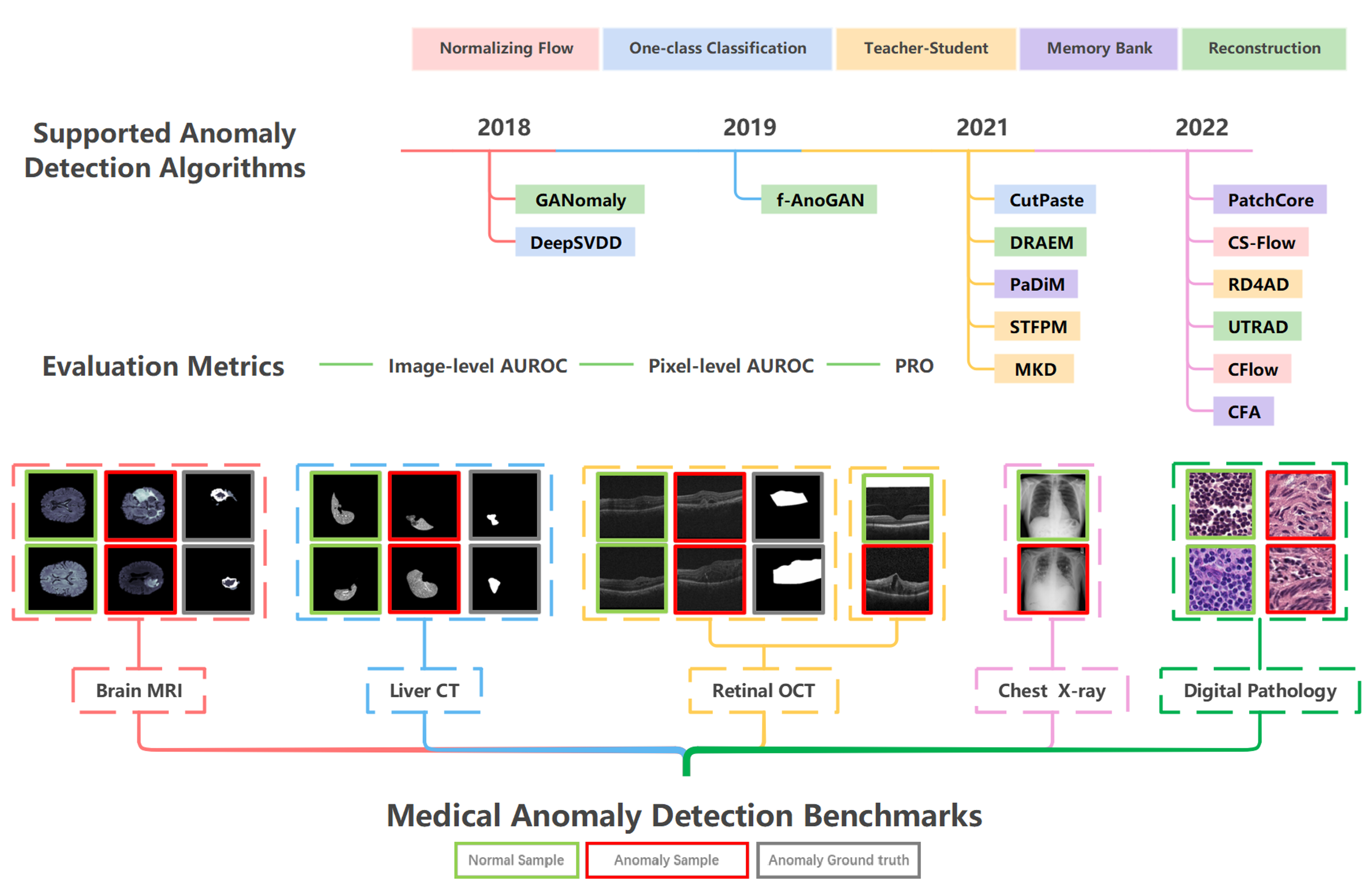
Figure 1: Diagram of the BMAD benchmarks. BMAD includes six medical datasets from five different domains for medical anomaly detection, among which three support pixel-level AD evaluation and the other three for sample-level assessment only. BMAD provides a well-structured and easy-used code base, integrating fourteen SOTA anomaly detection algorithms and three evaluation metrics.

To address the aforementioned issues, we introduce a uniform and comprehensive evaluation benchmark, namely BMAD, for assessing anomaly detection methods on medical images. This benchmark encompasses six well-reorganized datasets from five medical domains (i.e. brain MRI, liver CT, retinal OCT, chest X-ray, and digital histopathology) and three key evaluation metrics, and includes a total of fourteen state-of-the-art (SOTA) AD algorithms. This standardized and well-curated medical benchmark with the well-structured codebase enables comprehensive comparisons among recently proposed anomaly detection methods. Afterward, we evaluate the fourteen SOTA algorithms over the benchmarks and provides in-depth discussions on the results, which pinpoints potential research directions in future.

2 Related work

For unsupervised anomaly detection, the existing anomaly detection algorithms can be categorized into two paradigms: data reconstruction-based approaches and feature embedding-based (or projection-based) approaches. The former typically compares the differences between the reconstructed data and the original data in the data space to identify potential anomalies, while the latter infers anomalies by analyzing the abstract representations in the embedding space.

2.1 Reconstruction-based Methods

A reconstruction-based approach usually deploys a generative model for data reconstruction. It targets for small reconstruction residues for normal data, but large errors for anomalies. The distinction in reconstruction errors between normal and anomalous data forms the basis for anomaly detection. AutoEncoder (AE) and Variational AE have been the first and most popular models for this purpose [51, 76, 7, 50, 35, 21, 28, 40, 25, 78]. From the perspective of information theory, the bottleneck layer in the encoder-decoder architecture can be viewed as a constraint for information compression. During inference, it largely obstructs the passage of anomalous information. Later, Generative Adversarial Networks (GANs) are used to replace AE for its high-quality output [50, 41, 54, 1, 53, 67]. Recently, there is a trend of exploiting diffusion models for normal sample generation [64, 58, 63]. While convolutional neural networks have traditionally been the primary building block of these generative models, recent studies explore the transformer block instead [70, 27, 32, 16].

To improve AD performance, various regularization strategies are incorporated into normal sample reconstruction. Following the idea of denoising AE, Guassian noise is added into normal samples for a better normal data restoration performance [12, 13, 28]. In the masking mechanism, a normal sample is randomly masked and then inpainted back by a generative model [37, 73, 67]. Furthermore, many studies focus on synthesizing abnormalities on normal training samples and use the generative model to restore the original normal version [72, 20, 56]. Recently, the memory mechanism is exploited to further constrain model’s capability on reconstructing abnormal samples [21, 40, 25, 78].

2.2 Projection-based Methods

A projection-based method employs either a task-specific model or simply a pre-trained network to map data into abstract representations in an embedding space, enhancing the distinguishability between normal samples and anomalies. One-class classification usually uses normal support vectors/samples to define a compact closed one-class distribution. The one-class support vector machine [55] sought a kernel function to map the training data onto a hyperplane in the high-dimensional feature space. Any samples not on this hyperplane are considered anomalous samples. Similarly, support vector data description [57], DeepSVDD [49], and PatchSVDD [69] aimed to find a hyper-sphere enclosing normal data using either kernel-based methods or self-supervised learning. Teacher-student (T-S) architecture for knowledge distillation is a prevalent approach in AD recently [9, 14, 47, 52, 66, 19, 60]. It leverages a knowledgeable teacher model to distill its learned insights to a student network. Since the student network only learn representations of normal samples from the teacher, the representation discrepancy of the T-S pair forms the basis of anomaly detection. Memory Bank is a mechanism of remembering numerical prototypes of the training date [34, 18, 45, 31]. Then various algorithms such as KNN or statistical modeling are used to determine the labels for queries. Normalizing Flow is a method to explicitly model data distribution [44]. For AD, a flow model maps normal features onto a complex invertible distribution. The testing phase involves mapping normal samples to the trained distribution range, while abnormal samples are projected onto a separate distribution range [71, 48, 46, 22].

3 Benchmarks, Metrics, and Algorithms

Benchmarks	Originations	Total	Train	Test	Validation	Sample size	Annotation Level
Brain MRI	BraTS2021[3]	11,298 slices	7,500	3,715	83	240*240	Segmentation mask
Liver CT	BTCV [30] + LiTs [10]	3,201 slices	1,542	1,493	166	512*512	Segmentation mask
Retinal OCT	RESC[26]	6,217 images	4,297	1,805	115	512*1,024	Segmentation mask
	OCT2017 [29]	27,315 images	26,315	968	32	512*496	Image label
Chest X-ray	RSNA[62]	26,684 images	8,000	17,194	1,490	1,024*1,024	Image label
Pathology	Camelyon16 [6]	7,321 patches	5,088	1,997	236	256*256	Image label

Table 1: Summary of the six benchmarks from five imaging domains in BMAD.

3.1 Medical AD Benchmarks

BMAD includes six medical datasets from five different domains for medical anomaly detection. Within these datasets, three supports pixel-level evaluation of anomaly detection, while the remaining three is for sample-level assessment only. We summarize these benchmarks in Table 1. Note, the validation set is specifically designed for model hyper-parameter tuning and training strategy selection, while the test set should be remained untouched until the final evaluation stage.

Brain MRI AD Benchmark. Magnetic Resonance Imaging (MRI) imaging is widely utilized in brain tumor examination. The Brain MRI AD benchmark is reorganized using the flair modality of the latest large-scale brain lesion segmentation dataset, BraTS2021 [3]. Since the brain MRI scans of each patient comprises a complete 3D volume of the brain structure, we construct the benchmark from the 2D axial slices extracted from the 3D MRI scans. To refine the data quality, only slices within the depth range of 60-100 are included in the benchmark. Slices with lesions are labeled as anomaly and corresponding anomaly maps are obtained from the 3-D segmentation masks provided in BraTS2021 for anomaly localization assessment. In order to ensure data integrity, the dataset was carefully divided into distinct subsets for training, testing, and validation, with each subset containing non-overlapping patient IDs.

Liver CT AD Benchmark. Computed tomography (CT) is commonly used for abdominal examination. We structure this benchmark from two distinct datasets, BTCV [30] and Liver Tumor Segmentation (LiTs) set [10]. The anomaly-free BTCV set is initially proposed for multi-organ segmentation on abdominal CTs and taken to constitute the train set in this benchmark. CT scans in LiTs is exploited to form the evaluation and test data. For both datasets, Hounsfield-Unit (HU) of the 3D scans are transformed into grayscale with an abdominal window. The scans are then cropped into 2D axial slices, and the liver’s Region of Interest is extracted based on the provided organ annotations. We perform slide intensity normalization with histogram equalization. Slices with lesions, extracted from the LiTs dataset, are labeled as anomaly and the corresponding anomly masks are obtained from the groundtruth masks for liver tumors in LiTs.

Retinal OCT AD Benchmarks. Optical Coherence Tomography (OCT) is a commonly used imaging technique for scanning ocular lesions in eye pathology. To cover a wide range of anomalies and evaluate anomaly localization, we reorganize two benchmarks, Retinal Edema Segmentation Challenge dataset (RESC) [26] and Retinal-OCT dataset (OCT2017) [29]. RESC is initially proposed for retinal edema segmentation. We utilized the provided pixel-level ground truth to identify normal and abnormal samples. OCT2017 is a large-scale classification dataset originally. It contains three types of anomalies (CNV, DME, DRUSEN). We use the disease-free samples in the original training set as our training data and the entire test set of OCT2017 is divided into evaluation and testing data.

Chest X-ray AD Benchmark. X-ray imaging is a widely used method for examining the chest and provides precise thoracic data. The RSNA dataset [62] is originally provided to support the pneumonia detection challenge for supervised lung lesion detection. Based on the annotated labels in the original dataset, we categorized the samples into normal and abnormal data and proportionally split them into training, validation, and testing sets.

Digital Histopathology AD Benchmark. Histopathology involves the microscopic examination of tissue samples to study and diagnose diseases such as cancer. We utilize Camelyon16 [6], a digital pathology imaging breast cancer metastasis detection dataset, to build the histopathology benchmark. Camelyon16 contains 400 whole-slide images (WSIs), of which 159 contain tumor metastases. Since each WSI has 1 - 3 GB of data which is too large to be directly processed, we follow the prior arts and crop each WSI into small patches, with 256*256 size on 40× magnification [36, 59, 24]. Briefly, we randomly cropped 5,088 normal patches from the 160 normal WSIs in the original training set of Camelyon16, forming the training samples in the benchmark. For the validation set, we cropped 100 normal and 100 abnormal patches from the 13 testing WSIs. Similarly for testing, 1k normal and 1k abnormal patches were cropped from the 115 testing WSIs from the orignal Camelyon16 dataset.

Remark: Although this study focuses on unsupervised anomaly detection benchmarking, with only minor modifications on the evaluation set and training set, these benchmarks can also be used for weakly-supervised or even fully-supervised medical anomaly detection evaluation.

3.2 Evaluation Metrics

Anomaly detection can be evaluated from the sample level (i.e., detection rate) and the pixel level (i.e., anomaly localization). In BMAD, we take the area under the ROC curve (AUROC) as the numerical metric to quantify the sample-level and pixel-level AD performance. AUROC provides a quantitative value showing a trade-off between True Positive Rate (TPR) and False Positive Rate (FPR) across different decision thresholds. For sample-level AUROC, anomaly score is calculated based on the specific algorithm design and different thresholds are applied to determine if a sample is normal or abnormal. The obtained TPR and FPR pairs are recorded for estimating the ROC curve and AUROC value. To calculate the pixel-level AUROC, different thresholds are applied to the anomaly map. If a pixel has an anomaly score greater than the threshold, the pixel is anomalous. Over an entire image, the corresponding TPR and FPR pairs are used for numerical calculation. It should be noted that the TPR value in the ROC curve is biased by the size of defect areas. When larger abnormal regions are accurately localized, the TPR metric is noticeably improved. However, incorrect localization of smaller defect regions has a minimal impact on the metric. As a result, pixel-level AUROC has limitations to evaluate small tumor localization. To address this issue, we follow prior arts [8, 9, 19, 60] and include a threshold-independent metric, per-region overlap (PRO), to assess anomaly localization in BMAD. PRO treats anomaly regions of different size equally, upweighting the influence of small-size abnormality localization in final evaluation. Specifically, for each threshold, detected anomalous pixels are grouped into connected components and PRO is calculated by averaging localization accuracy over all components.

3.3 Supported AD Algorithms

BMAD integrates fourteen SOTA anomaly detection algorithms, among which four are reconstruction-based methods and the rest ten algorithms are feature embedding-based approaches. AnoGAN [54] and f-AnoGAN [53] are popular approaches for medical anomaly detection. They exploit the GAN architecture to generate normal samples. DRAEM [72] consists of two networks, one for abnormality inpainting and the other for anomaly classification. The former adopts an encoder-decoder architecture and is trained to restore the abnormal synthesis; the latter takes the original data and the inpainting result as input for binary classification. UTRAD [16] treated the deep pre-trained features as dispersed word tokens and construct an autoencoder with transformer blocks. Among the projection-based methods, DeepSVDD [49] and CutPaste [33] is rooted in one-class classification. DeepSVDD [49] utilizes a neural network to extract numerical features and then searches a smallest hyper-sphere to enclose these normal embeddings. CutPaste[33] introduces a simple yet effective abnormality synthesis algorithm to extend the one-class classification, where generated abnormality synthesis is taken as negative samples in model training. Motivated by the paradigm of knowledge distillation, MKD [52] and STFPM [66] leverage multi-scale feature discrepancy between the teacher-student pair for AD. Instead of adopting the similar backbones for the T-S pair in knowledge distillation, RD4AD [19] introduced a novel architecture consisting of a teacher encoder and a student decoder, which significantly enlarges the representation dissimilarity for anomaly samples. All of PaDiM [18], PatchCore [45] and CFA [31] rely on a memory bank to store normal prototypes. Specifically, PaDiM[18] utilizes a pre-trained model for feature extraction and models the obtained features using a Gaussion distribution. PatchCore[45] leverages core-set sampling to construct a memory bank and adopts the nearest neighbor search to vote for a normal or abnormal prediction. CFA[31] improves upon PatchCore by creating the memory bank based on the distribution of image features on a hyper-sphere. As notable from the name, CFlow [22] and CS-Flow [48] are flow-based methods. The former introduced positional encoding in conjunction with a normalizing flow module and the latter incorporates multi-scale features for distribution estimation.

4 Experiments and Discussions

4.1 Implementation Details

When evaluating the fourteen AD algorithms over the benchmarks in BMAD, we follow their original papers and try their default hyper-parameter settings first. If a model doesn’t converge during training and requires hyper-parameter tuning, we try the combination of following common settings, which include 3 learning rate ($10^{-3}$,$10^{-4}$ and $10^{-5}$), 2 optimizer (SGD and Adam), and 3 thresholds for anomaly maps (0.5, 0.6, and 0.7). To ensure fairness, we established a standardized evaluation procedure for all models. Briefly, we monitor a model’s training progress and record the validation accuracy every 10 epochs. The final evaluation is carried out on the test set using the best checkpoint selected from recorded validation results. To visualize the results of anomaly localization, we employ min-max normalization on the obtained anomaly maps. This technique ensures that the effects of all algorithms are appropriately displayed and facilitates the comparison of anomaly localization across different methods. Notably, for a reliable comparison, we repeat the training and evaluation three times, each with a different random seed, and report the mean and standard deviation of the numerical metrics. All experiments are performed on a workstation with 2 NVIDIA RTX 3090 cards.

Benchmarks

BraTS2021

BTCV + LiTs

RESC

OCT2017

RSNA

Camelyon16

Image

Pixel

Pixel

Image

Pixel

Pixel

Image

Pixel

Pixel

Image

Image

Image

AUROC

AUROC

Pro

AUROC

AUROC

Pro

AUROC

AUROC

Pro

AUROC

AUROC

AUROC

Image Reconstruction-based Methods

f-AnoGAN [53]

$77.36\pm 0.08$

NA

NA

$58.35\pm 0.15$

NA

NA

$77.05\pm 0.43$

NA

NA

$72.84\pm 1.12$

$55.1\pm 0.04$

$69.24\pm 1.74$

GANomaly [1]

$74.58\pm 1.72$

NA

NA

$53.89\pm 2.36$

NA

NA

$51.7\pm 3.35$

NA

NA

$68.6\pm 9.58$

$62.85\pm 0.61$

$53.59\pm 1.77$

DRAEM [72]

$62.45\pm 9.03$

$81.77\pm 3.96$

$62.18\pm 4.06$

$69.23\pm 3.86$

$87.82\pm 3.23$

$78.99\pm 5.66$

$81.62\pm 8.14$

$86.02\pm 3.14$

$64.07\pm 5.0$

$86.07\pm 10.46$

$67.49\pm 1.9$

$52.30\pm 0.81$

UTRAD[16]

$82.18\pm 2.61$

$92.55\pm 0.72$

$71.8\pm 2.43$

$55.63\pm 5.96$

$87.83\pm 1.35$

$70.38\pm 3.76$

$88.97\pm 2.01$

$94.67\pm 1.04$

$77.47\pm 4.28$

$96.85\pm 0.67$

$75.34\pm 0.94$

$69.32\pm 4.44$

Image Feature-based methods

DeepSVDD [49]

$86.82\pm 0.46$

NA

NA

$53.3\pm 1.24$

NA

NA

$73.98\pm 1.16$

NA

NA

$79.02\pm 1.17$

$64.73\pm 3.48$

$61.14\pm 2.02$

CutPaste [33]

$78.75\pm 0.56$

NA

NA

$58.58\pm 4.2$

NA

NA

$90.26\pm 0.64$

NA

NA

$96.78\pm 0.64$

$82.42\pm 1.02$

$75.23\pm 0.47$

MKD [52]

$81.38\pm 0.27$

$89.54\pm 0.34$

$67.46\pm 0.86$

$60.39\pm 1.61$

$96.14\pm 0.35$

$91.06\pm 0.32$

$88.97\pm 0.2$

$86.6\pm 0.51$

$65.87\pm 1.21$

$96.62\pm 0.22$

$81.99\pm 0.1$

$77.74\pm 0.07$

RD4AD[19]

$89.38\pm 0.97$

$96.54\pm 0.06$

$85.86\pm 0.23$

$60.02\pm 1.4$

$95.86\pm 1.02$

$90.13\pm 2.35$

$87.53\pm 0.62$

$96.17\pm 0.15$

$85.78\pm 0.52$

$97.24\pm 0.73$

$67.53\pm 1.21$

$66.59\pm 0.91$

STFPM[66]

$82.88\pm 0.87$

$95.75\pm 0.25$

$82.62\pm 0.84$

$61.57\pm 1.7$

$90.98\pm 5.72$

$89.28\pm 7.14$

$84.48\pm 0.72$

$94.57\pm 0.68$

$81.34\pm 1.67$

$90.12\pm 0.53$

$69.24\pm 1.56$

$66.06\pm 1.31$

PaDiM [18]

$78.62\pm 0.78$

$95.62\pm 0.23$

$81.59\pm 0.54$

$50.67\pm 0.50$

$90.46\pm 0.37$

$76.71\pm 0.36$

$75.73\pm 0.42$

$91.38\pm 0.36$

$71.52\pm 0.97$

$91.53\pm 0.74$

$75.93\pm 0.37$

$67.11\pm 0.46$

PatchCore[45]

$91.55\pm 0.46$

$96.97\pm 0.04$

$85.83\pm 0.16$

$60.40\pm 0.82$

$96.58\pm 0.04$

$87.35\pm 0.74$

$91.50\pm 0.05$

$96.39\pm 0.07$

$85.73\pm 0.36$

$98.56\pm 0.03$

$75.17\pm 0.97$

$69.34\pm 0.17$

CFA [31]

$84.65\pm 1.05$

$96.40\pm 0.07$

$83.62\pm 0.67$

$61.94\pm 1.16$

$97.21\pm 0.17$

$92.55\pm 0.24$

$69.91\pm 0.26$

$91.06\pm 0.91$

$69.69\pm 0.33$

$79.17\pm 0.86$

$66.62\pm 0.04$

$65.60\pm 0.14$

CFLOW [22]

$73.97\pm 4.93$

$93.52\pm 0.93$

$75.01\pm 3.11$

$49.93\pm 4.67$

$92.78\pm 1.36$

$82.92\pm 1.48$

$74.43\pm 5.41$

$93.75\pm 0.54$

$76.76\pm 1.76$

$85.43\pm 2.02$

$71.44\pm 1.58$

$54.54\pm 1.27$

CS-Flow [48]

$90.91\pm 0.81$

NA

NA

$59.39\pm 0.52$

NA

NA

$87.1\pm 0.41$

NA

NA

$98.75\pm 0.08$

$83.24\pm 0.5$

$68.47\pm 0.33$

Table 2: AD performance comparison over the benchmarks in BMAD. The top three methods for each metric are underlined. NA indicates that a method doesn’t support anomaly localization.

Figure 2: Visualization examples of anomaly localization on the three benchmarks that support pixel-level AD assessment.

4.2 Results and Discussions

Experimental result overview. The numerical results of anomaly detection and localization over the BMAD benchmark are summarized in Table 2, where the top three performance along each metric are highlighted by underlining. We also provide visualization examples of anomaly localization results in Fig. 2, where redness corresponds to a high anomaly score at the pixel level. Although no single algorithm consistently outperforms others, overall, the feature-based methods shows better performance than the reconstruction-based methods. We believe that two reasons may lead to this observation. First, applying generative models to anomaly detection usually relies on model’s reconstruction residue in the pixel level. However, a well-trained generative model usually has good generalizability and it has been found in prior arts that certain anomalous regions can be well reconstructed. This issue hurts anomaly detection performance. Second, reconstruction residue in the pixel level may not well reflect the high-level, context abnormalities. In contrast, algorithms detecting abnormalities from the latent representation domain (such as RD4AD [19], PatchCore [45], etc.) facilitate identifying abstract structural anomalies. Therefore, these algorithms perform much better than the generative models. It should be noted that for benchmarks like Liver CT and Brain MRI, where the background consists mostly of black pixels and the distribution of normal and anomalous samples is imbalanced, the numerical results exist bias. Therefore, a high pixel-level AUROC score may indicate that the model correctly classifies the majority of normal pixels, but it does not necessarily reflect the model’s ability to detect anomalies accurately. Besides, we have several interesting observations through this research that necessitate careful analysis in order to advance the field of medical anomaly detection. We elaborate our insights and discoveries as follows.

Anomaly localization analysis. By incorporating anomaly segmentation into the evaluation process, we can gain more comprehensive insights into various anomaly detection methods. Since different approaches generate the anomaly map in various ways, either relying on reconstruction error [19, 61, 72, 16], using gradient-based visualization [52, 45], or measuring feature discrepancy [18, 22, 31], they shows distinct advantages and limitations. Generally speaking, both numerical data in Table 1 and the visualization results in Fig. 2 demonstrate that knowledge-distillation methods, especially RD4AD [19], achieve better localization performance. Although memory bank-based algorithm, Patchcore [45], is more convincing at sample-level detection, its abnormality localization is very coarse. Reconstruction-based algorithms, DRAEM [72] and UTRAD [16], shows diverse performance. We hypothesize their distinct capability of anomaly localization is attributed to the different architecture of CNN and transformer. We notice that DRAEM [72] is particularly sensitive to texture information, often focusing on regions with significant variations in tumor texture. Since such variations may be distributed across all regions in medical imaging, it partially limits the effectiveness of the proposed approach. CFlow [22] shows bad anomaly localization performance and more investigation is needed for its improvement.

Model efficiency analysis. For all fourteen algorithms, we conduct a comparative efficiency analysis, in terms of sample-level AD accuracy, inference speed and GPU usage, on BMAD and summarize the comparison in Fig 3. The X-axis refers to the inference time for each image and Y-axis denotes the performance of the anomaly detection result. The size of the circle denotes the GPU memory consumption during the inference phase. PatchCore [45], RD4AD [19], and CS-FLOW [48] emerge as the top 3 models across multiple benchmarks in terms of performance. It should be noted that though CS-Flow demonstrates comparable inference time to the other two models, it has lower efficiency to generate pixel-lever anomaly maps.

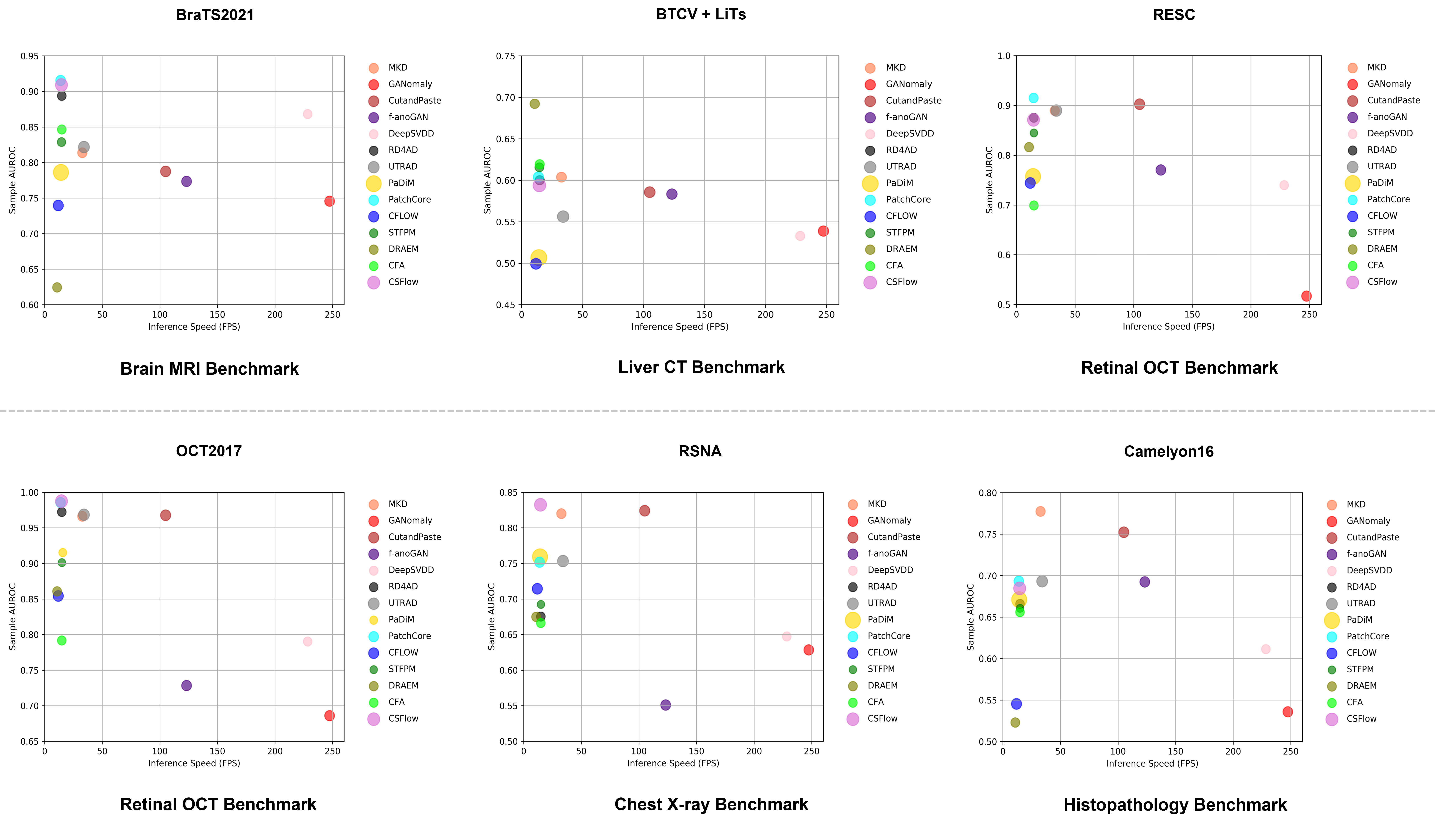
Figure 3: Experiment on Model Efficiency. Visualization of all algorithms on sample-level AUROC, inference time and GPU memory under each benchmark. X-axis refers to the inference time for each image and Y-axis denotes the performance of the anomaly detection result. The size of the circle denotes the GPU memory consumption during the inference phase. A higher Image AUROC indicates a higher level of model accuracy. Inference time FPS (frames per second) is inversely proportional to model efficiency. A higher FPS indicates higher model efficiency. In the sub-images, there may be slight variations in the results due to unique adjustments made during the fine-tuning process of each algorithm. These adjustments involve selecting specific parameters and backbones to optimize performance for specific benchmark. Our goal is to achieve the best performance for every algorithm.

Anomaly synthesis is challenging. In unsupervised AD methods, one common approach is to synthesize abnormalities to augment model training. CutPaste [33] and DRAEM [72] are the examples. However, to address the variability in shape, texture, and color of medical anomalies across different domains, a customized synthesis algorithm is needed to simulate realistic tumor lesions and their distributions. It is important to acknowledge the inherent difficulty in simulating the morphology of anomalies, and this challenge becomes even more pronounced when considering rare diseases. We discovered that the Brain MRI and Liver CT benchmarks are better suited for low-level feature-based anomaly augmentation methods. This observation aligns with the characteristics of the Chest X-ray and Histopathology benchmarks, where abnormalities often exhibit distinct and observable changes in overall structure or appearance. Therefore, it is essential to develop domain-specific approaches that account for these factors when augmenting anomalies in medical image datasets.

Pre-trained networks significantly contribute to medical domain. Through there is a continuous debate on if information obtained from natural images is transferable to medical image analysis, our results show that the rich representations of pre-trained models would improve medical anomaly detection by careful algorithm design. Among the models evaluated, algorithms based on the knowledge-distillation paradigm (e.g. MKD [52] and RD4AD [19]) and memory bank (e.g. Patchcore [45]) leverage the powerful feature extraction capabilities of large pre-train models and exhibit better performance in anomaly localization, which plays a crucial role in clinical diagnosis.

Memory bank-based methods have shown promising performances. PatchCore[45] is a representative example. These methods possess the ability to incorporate new memories, effectively mitigating forgetting when learning new tasks. Hence, the memory bank serves as an ideal rehearsal mechanism. However, these methods have specific hardware requirements to ensure efficient storage and retrieval of stored information. Achieving high-capacity storage systems and efficient memory access mechanisms for optimal performance while minimizing interference time presents a notable challenge. Furthermore, our observations indicate that memory-based methods, while sensitive to global anomalies, may not excel in terms of localizing and visualizing anomalies when compared to feature reconstruction methods. Accurate anomaly localization holds crucial practical value for AD algorithms and provides valuable insights to medical professionals. Therefore, memory bank-based methods may encounter challenges and limitations that impact their competitiveness in certain scenarios.

Model degradation problem. The model degradation problem occurs when a deep neural network, trained on a large dataset, exhibits degraded performance as the network’s depth increases. We have also found that model degradation issues also exist in BMAD. However, it is a challenge to add appropriate preprocessing and data augmentation techniques to medical benchmarks. Additionally, we believe that incorporating adversarial training for medical data can be a viable approach to enhance the robustness of the models.

5 Outlook and Conclusion

Conclusion. In this study, we presented a comprehensive medical anomaly detection benchmark that encompasses six distinct benchmarks derived from five major medical domains. The benchmark integrated fourteen SOTA AD algorithms, covering all major AD algorithm design paradigms. To ensure a thorough evaluation, we assessed the performance of these algorithms from multiple comparison perspectives, as detailed in the paper. This benchmark stands as the most extensive collection thus far, offering a comprehensive evaluation framework for medical AD algorithms.

Limitation and Feature work. While we compared representative algorithms in this study, we acknowledge that there are other recently released or emerging algorithms that were not included. In the future, we plan to extend and supplement the benchmark with relevant algorithms to maintain its relevance and comprehensiveness.

Social Impact. Unified benchmarks in the medical field play a crucial role in establishing better standards and support for medical anomaly detection work. Particularly in the case of medical anomaly detection, a lack of a unified benchmark hinders fair evaluations of anomaly detection algorithms. Our contributions address this gap by consolidating disparate medical benchmarks and integrating imperfect anomaly detection methods in the medical domain. This provides a valuable reference for both general anomaly detection methods and researchers in the medical field. Furthermore, we put forth several compelling directions for future research in medical image anomaly detection, which will greatly benefit the entire community and guide future work in this area. It should be noted that since unsupervised anomaly detection relies on normal data collected for model training, there are fairness and ethical concerns if the collected data involves biases. Such negative social impacts should be addressed in data collection for AD.

Appendix A BMAD datasets

Our BMAD benchmark consists of six datasets sourced from five distinct medical domains, including brain MRI, retinal OCT, liver CT, chest X-ray, and digital histopathology. Due to the absence of specific anomaly detection datasets in the field of medical imaging, we construct these benchmark datasets by reorganizing and remixing existing medical image sets proposed for other purposes such as image classification and segmentation. These reorganized datasets are readily available for download via our BMAD Github page at https://github.com/DorisBao/BMAD. Moreover, our codebase includes functionality for data reorganization, enabling users to generate new datasets tailored to their needs. In the this sections, we mainly focus on an overview of the original datasets and our data reorganization procedure.

A.1 Brain MRI Anomaly Detection and Localization Benchmark

The brain MRI anomaly detection benchmark is reorganized from the BraTS2021 dataset [3, 38, 4].

A.1.1 BraTS2021 Dataset

The original BraTS2021 dataset is proposed for a multimodel brain tumor segmentation challenge. It provides 1,251 cases in the training set, 219 cases in validation set, 530 cases in testing set (nonpublic), all stored in NIFTI (.nii.gz) format. Each sample includes 3D volumes in four modalities: native (T1) and post-contrast T1-weighted (T1Gd), T2-weighted (T2), and T2 Fluid Attenuated Inversion Recovery (T2-FLAIR), accompanied by a 3D brain tumor segmentation annotation. The data size for each modality is 240 *240 *155.

Access and License: The BraTS2021 dataset can be accessed at http://braintumorsegmentation.org/. Registration for the challenge is required. As stated on the challenge webpage, "Challenge data may be used for all purposes, provided that the challenge is appropriately referenced using the citations given at the bottom of this page."

A.1.2 Construction of Brain MRI AD benchmark

After analyzing the BraTS2021 dataset, we built the brain MRI AD benchmark from the 3D FLAIR volumes. All data in our Brain MRI AD benchmark is derived from the 1,251 cases in the original training set. To account for variations in brain images at different depths, we specifically selected slices within the depth range of 60 to 100. Each extracted 2D slice was saved in PNG format and has an image size of 240 * 240 pixels. According to the tumer segmentation mask, we selected 7,500 normal samples to compose the AD training set, 3,715 samples containing both normal and anomaly samples (with a ratio of 1:1) for the test set, and a validation set with 83 samples that do not overlap with the test set. Fig. 4 illustrates the specific procedure we followed for data preparation, and Fig. 5 provides examples of our brain MRI AD benchmark.

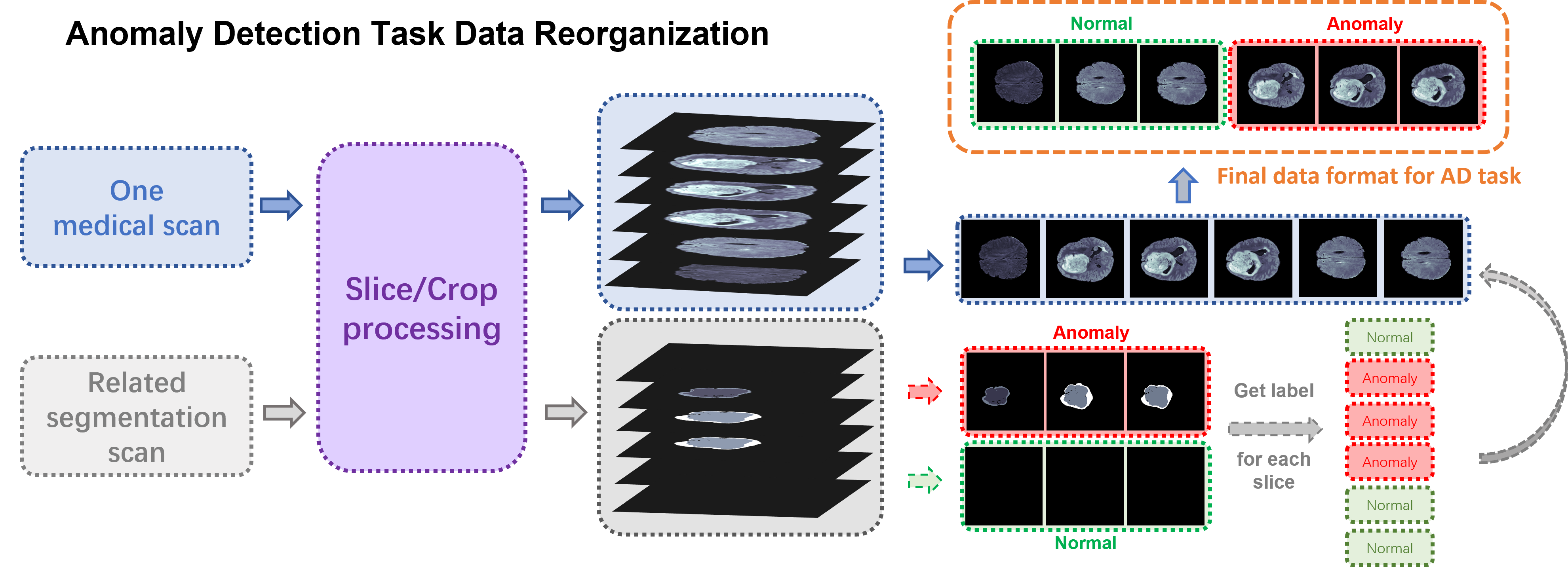
Figure 4: Diagram illustration of data preparation for the Brain MRI AD benchmark from 3D brain scans in BraTS2021.

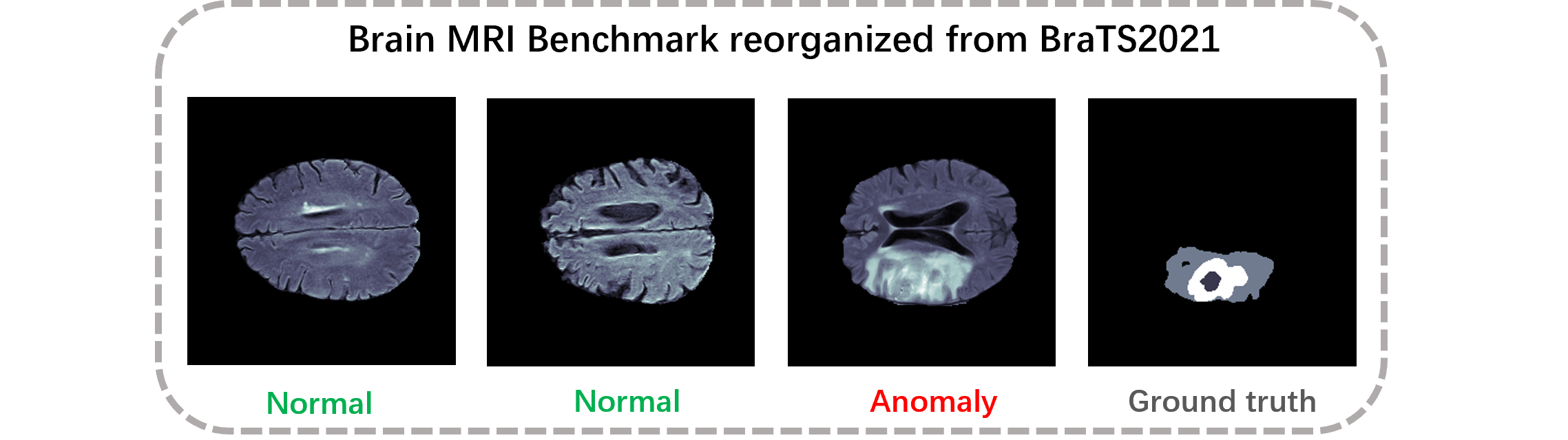
Figure 5: Visualization of our proposed Brain MRI benchmark.

A.2 Liver CT Anomaly Detection and Localization Benchmark

We structure this benchmark from two distinct datasets, BTCV [30] and LiTS [10]. The anomaly-free BTCV set is taken to constitute the normal train set in this benchmark and CT scans in LiTs is exploited to form the evaluation and test data.

A.2.1 BTCV Dataset

BTCV [30] is introduced for multi-organ segmentation. It consists of 50 abdominal computed tomography (CT) scans taken from patients diagnosed with colorectal cancer and a retrospective ventral hernia. The original scans were acquired during the portal venous contrast phase and had variable volume sizes ranging from 512*512*85 to 512*512*198 and stored in nii.gz format.

Access and License: The original BTCV dataset can be accessed from ’RawData.zip’ at https://www.synapse.org/#!Synapse:syn3193805/wiki/217753. Dataset posted on Synapse is subject to the Creative Commons Attribution 4.0 International (CC BY 4.0) license.

A.2.2 LiTS Dataset

LiTS[10] is proposed for liver tumor segmentation. It originally comprises 131 abdominal CT scans, accompanied by a ground truth label for the liver and liver tumors. The original LiTS is stored in the nii.gz format with a volume size of 512*512*432.

Access and License: LiTS can be downloaded from its Kaggle webpage at https://www.kaggle.com/datasets/andrewmvd/liver-tumor-segmentation. The use of the LiTS dataset is under Creative Commons Attribution-NonCommercial-ShareAlike(CC BY-NC-SA)[11].

A.2.3 Construction of Liver CT AD Benchmark

In constructing the liver CT AD benchmark, we made a decision not to include lesion-free regions from the LiTS dataset as part of the training set. This choice was based on our observation that the presence of liver lesions in LiTS leads to morphological changes in non-lesion regions, which could impact the performance of anomaly detection. Instead, we opted to use the lesion-free liver portion from the BTCV dataset to form the training set. The LiTS dataset, on the other hand, is reserved for testing the effectiveness of anomaly detection and localization.

For both datasets, Hounsfield-Unit (HU) of the 3D scans are transformed into grayscale with an abdominal window. The scans are then cropped into 2D axial slices, and the liver’s Region of Interest is extracted based on the provided organ annotations. We perform slide intensity normalization with histogram equalization. To be more specific, for the construction of the normal training set in the liver CT AD benchmark, we utilized the provided segmentation labels in BTCV to extract the liver region. From these scans, we extracted 2D slices of the liver with a size of 512 * 512, using the corresponding liver segmentation scans as a guide. The 2D slices were then converted to PNG format to serve as the final AD data. We selected 1542 slices to comprise the training set. To prepare the testing and validation sets, we sliced the data from LiTS and stored them in PNG format with dimensions of 512 * 512. Our testing and validation sets contain both healthy and abnormal samples. Fig. 6 demonstrates several samples in the Liver CT AD dataset. Fig. 6 provides visualization of the constructed Liver CT AD dataset.

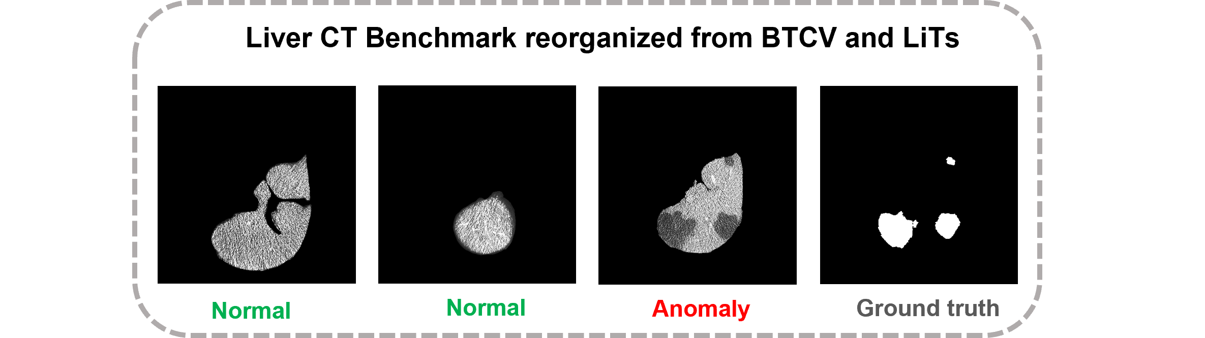
Figure 6: Visualization of our proposed Liver CT benchmark.

A.3 Retinal OCT Anomaly Detection and Localization Benchmark

The BMAD datasets includes two different OCT anomaly detection datasets. The first one is derived from the RESC dataset [26] and support anomaly localization evaluation. The second is constructed from OCT2017[29], Which only support sample-level anomaly detection.

A.3.1 RESC dataset

RESC (Retinal Edema Segmentation Challenge) dataset [26] specifically focuses on the detection and segmentation of retinal edema anomalies. It provides pixel-level segmentation labels, which indicate the regions affected by retinal edema. The RESC is provided in PNG format with a size of 512*1024 pixels.

Access and License: The original RESC dataset can be downloaded from the P-Net github page at https://github.com/CharlesKangZhou/P_Net_Anomaly_Detection. As indicated on the webpage, the dataset can be only used for the research community.

A.3.2 OCT2017 dataset

OCT2017 [29] is a large-scale dataset initially designed for classification tasks. It consists of retinal OCT images categorized into three types of anomalies: Choroidal Neovascularization (CNV), Diabetic Macular Edema (DME), and Drusen Deposits (DRUSEN). The images are continuous slices with a size of 512*496.

Access and License: OCT2017 can be downloaded at https://data.mendeley.com/datasets/rscbjbr9sj/2. Its usage is under a license of Creative Commons Attribution 4.0 International(CC BY 4.0).

A.3.3 Preparation of OCT AD benchmarks

To construct the OCT anomaly detection and localization dataset from RESC, we utilize the segmentation labels provided for each slice to get the label for AD setting. We select the normal samples from the original training dataset and adapt the original validation set into the AD setting for evaluation. The RESC is provided in PNG format with a size of 512*1024 pixels. On the other hand, on the OCT2017 dataset, we specifically select the disease-free samples from the original training set as our training data for the anomaly detection task. The test set is further divided into evaluation data and testing data for AD setting. Fig. 7 demonstrates several examples in the two OCT AD datasets.

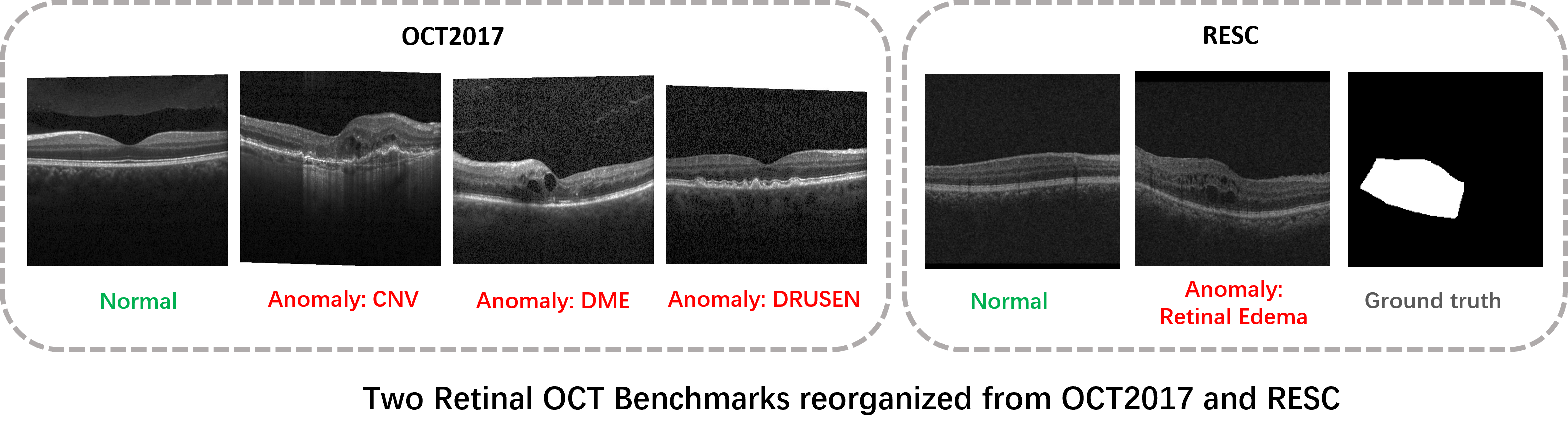
Figure 7: The Retinal OCT benchmarks consist of two separate datasets, each representing different anomaly types. These datasets are used to evaluate and benchmark various methods in the field of retinal OCT imaging. The datasets are designed to assess the performance of algorithms in detecting and localizing specific anomalies in retinal images.

A.4 Chest X-ray Anomaly Detection Benchmark

A.4.1 RSNA dataset

RSNA[62], short for RSNA Pneumonia Detection Challenge, is originally provided for a lung pneumonia detection task. The 26,684 lung images are associated with three labels: "Normal" indicates a normal lung condition, "Lung Opacity" indicates the presence of pneumonia, "No Lung Opacity/Not Normal" represents a third category where some images are determined to not have pneumonia, but there may still be some other type of abnormality present in the image. All images in RSNA are in DICOM format.

Access and License: RSNA can be accessed by https://www.kaggle.com/competitions/rsna-pneumonia-detection-challenge/overview. Stated in the section of Competition data: A. Data Access and Usage, "… you may access and use the Competition Data for the purposes of the Competition, participation on Kaggle Website forums, academic research and education, and other non-commercial purposes."

A.4.2 Preparation of Chest X-ray AD Benchmark

We utilized the provided image labels for data re-partition. Specifically, "Lung Opacity" and "No Lung Opacity/Not Normal" were classified as abnormal data. The reorganized AD dataset including 8000 normal images as training data, 1490 images with 1:1 normal-versus-abnormal ratio in the validate set, and 17194 images in the test set. Examples of the chest X-ray dataset are provided in Fig. 8.

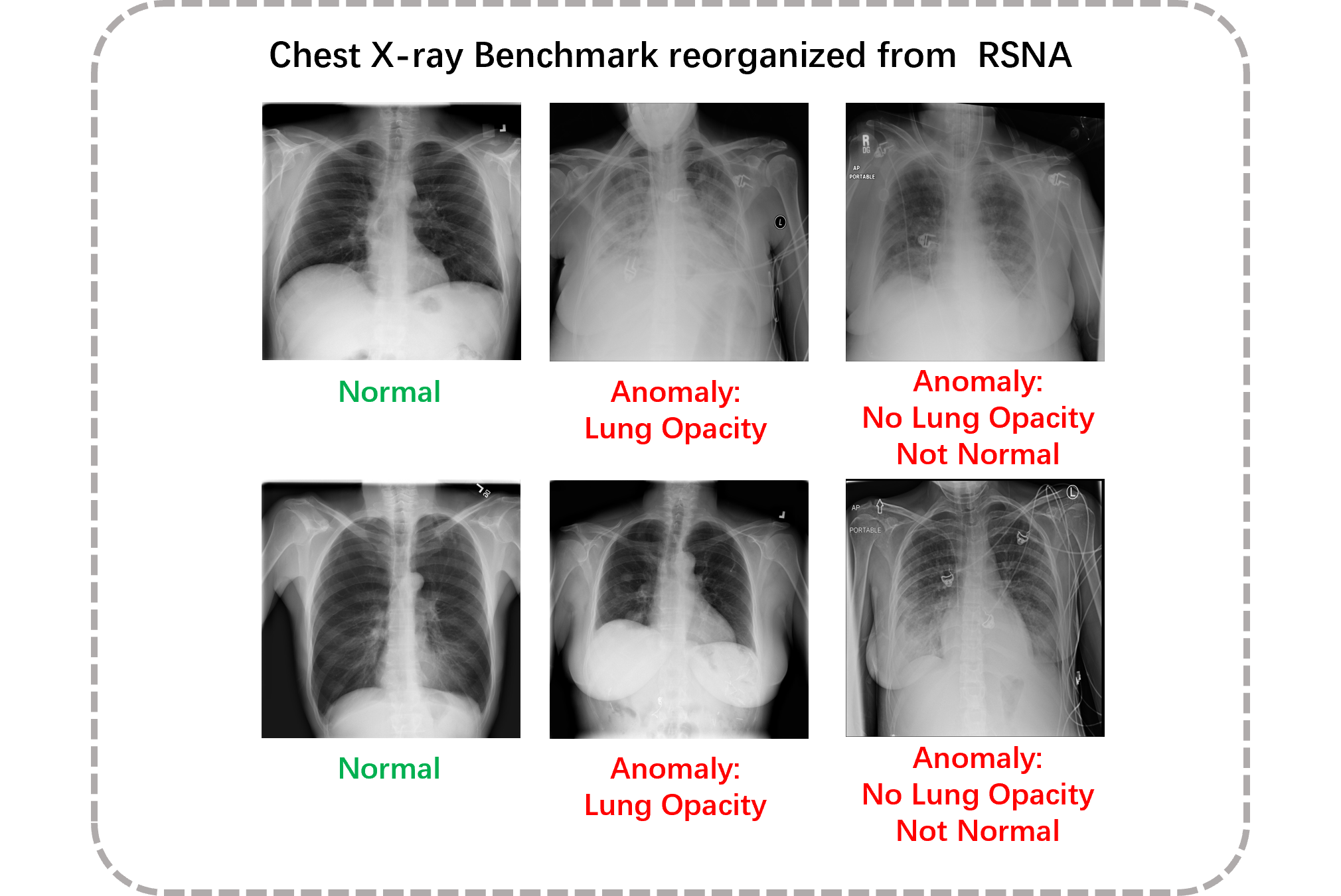
Figure 8: Our proposed chest X-ray benchmark consists two types of anomalies. These anomalies are clearly labeled in the images, and all of them are considered as anomaly samples.

A.5 Digital Histopathology Anomaly Detection Benchmark

A.5.1 Camelyon16 Dataset

The Camelyon16 dataset [6] was initially utilized in the Camelyon16 Grand Challenge to detect and classify metastatic breast cancer in lymph node tissue. It comprises 400 whole-slide images (WSIs) of lymph node sections stained with hematoxylin and eosin (H&E) from breast cancer patients. Among these WSIs, 159 of them exhibit tumor metastases, which have been annotated by pathologists. The WSIs are stored in standard TIFF files, which include multiple down-sampled versions of the original image. In Camelyon16, the highest resolution available is on level 0, corresponding to a magnification of 40X.

Access and Licence: The original Camelyon16 dataset can be found at https://camelyon17.grand-challenge.org/Data/. It is under a license of Creative Commons Zero 1.0 Universal Public Domain Dedication(CC0).

A.5.2 Preparation of histopathology AD Benchmark

To ensure a comprehensive evaluation of anomaly detection models for histopathology images, considering their unique characteristics such as large size, we opted to assess AD models at the patch level. To construct the benchmark dataset, we randomly extracted 5,088 normal patches from the original training set of Camelyon16, which consisted of 160 normal WSIs. These patches were utilized as training samples. For the validation set, we cropped 100 normal and 100 abnormal patches from the 13 testing WSIs. Likewise, for the testing set, we extracted 1,000 normal and 1,000 abnormal patches from the 115 testing WSIs in the original Camelyon16 dataset. Each cropped patch was saved as a PNG image with dimensions of 256 * 256 pixels. Fig. 9 presents several examples in the constructed histopathology AD benchmark.

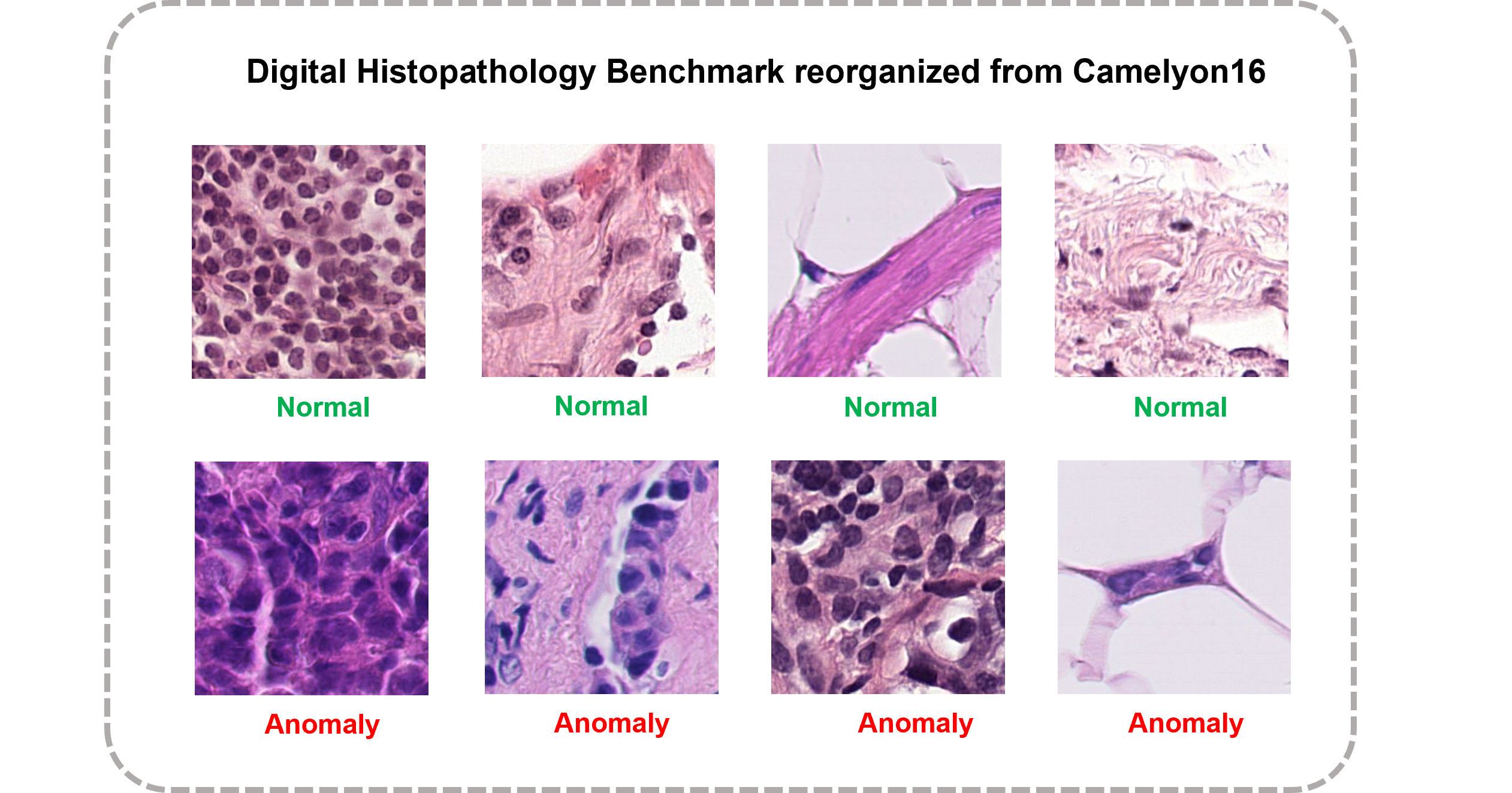
Figure 9: Examples of the digital histopathology AD benchmark. Unlike other medical image AD benchmarks, histopathology images shows higher diversities in tissue components.

A.6 Remarks on Benchmark datasets

We observed that there were biases present in the original datasets, which may impact the performance of the models. For instance, in the chest dataset, the results may be influenced by the uneven gender distribution. Additionally, in the liver CT benchmark, the performance can be affected by the bias introduced by the cropped area.

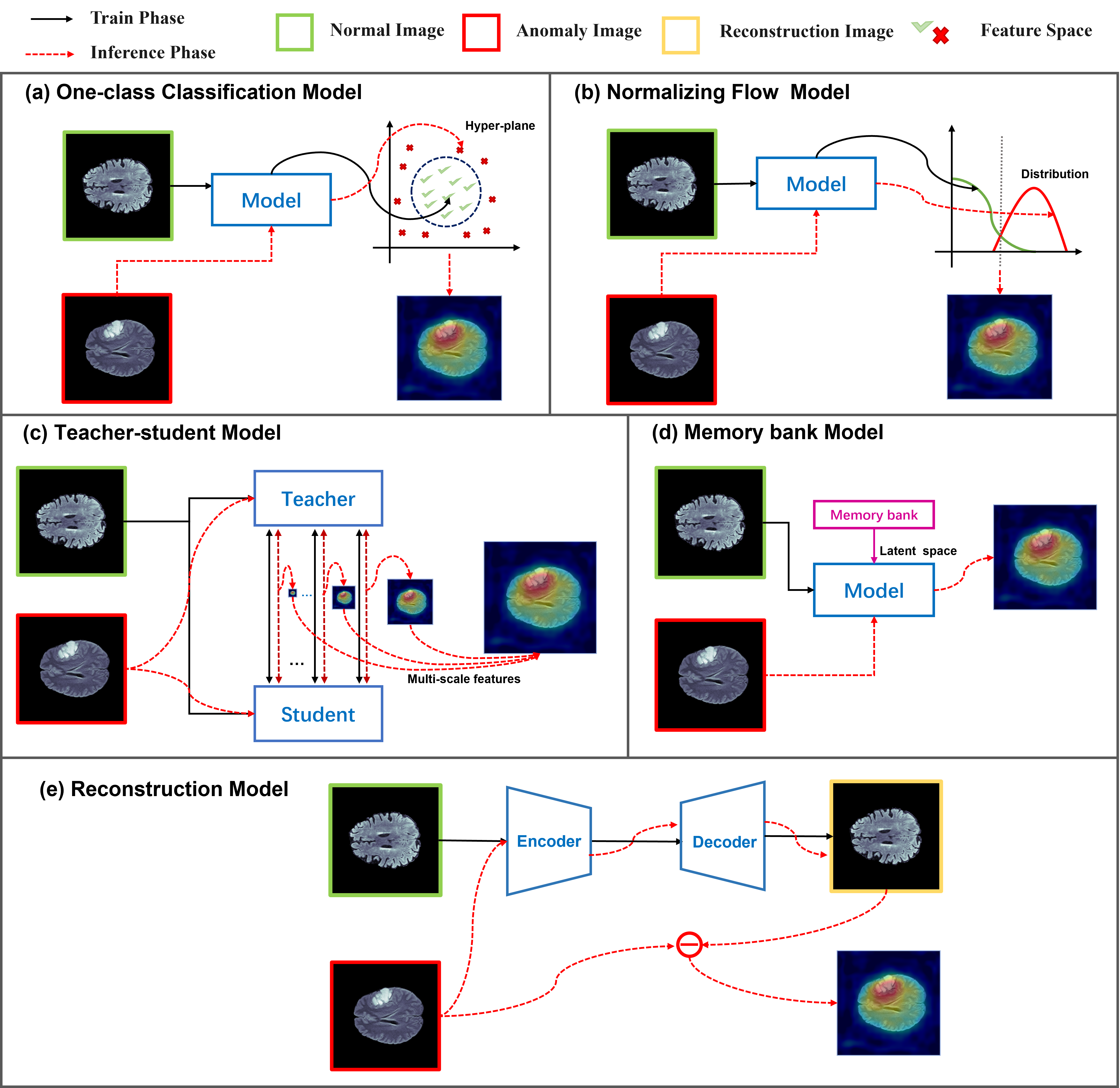
Figure 10: Conceptual illustration of various AD models. The one-class classification model, normalizing flow model, teaching-student model and memory bank model detects anomalies in the embedding space, and the reconstruction based method takes a generative model as its backbone for pixel-level anomaly comparison between the original query and reconstruction.

Appendix B Supported AD Models

Fig. 10 provides conceptual illustration of various AD architectures from the feature embedding-based methods and data reconstruction-based approaches. The specific experimental settings for each of the supported methods are specified as follows.

PaDiM [18] leverages a pre-trained convolutional neural network (CNN) for its operations and does not require additional training. In our experiments, we separately evaluated all benchmarks using two backbone networks: ResNet-18 and WideResnet-50. For the dimension reduction step, we retained the default number of features as specified in the original setting. Specifically, we used 100 features for ResNet-18 and 550 features for WideResnet-50. These default values were chosen based on the original implementation and can serve as a starting point for further experimentation and fine-tuning if desired.

STFPM[66] utilized feature extraction from a Teacher-student structure. In our experiments, we evaluated all benchmarks separately using two backbone networks: ResNet-18 and WideResnet-50. We employed a SGD optimizer with a learning rate of 0.4. Additionally, we followed the original setting with a parameter with a momentum of of 0.9 and weight decay of 1e-4 for SGD. These settings were chosen based on the original implementation and can be adjusted for further experimentation if desired.

Patchcore[45] is a memory-based method that utilizes coreset sampling and neighbor selection. In our experiments, we evaluated Patchcore using two backbone networks: ResNet-18 and WideResnet-50. We followed the default hyperparameters of 0.1 for the coreset sampling ratio and 9 for the chosen neighbor number. These values were chosen based on the original implementation.

RD4AD[19] utilizes a wide ResNet-50 as the backbone network and applies the Adam optimizer with a learning rate of 0.005. In addition, we follow the defeat set of the beta1 and beta2 parameters to 0.5 and 0.99, respectively. For the anomaly score of each inference sample, the maximum value of the anomaly map is used. These settings were determined based on the original implementation of RD4AD and can be adjusted if needed.

DRAEM[72] is a anomaly augmentation reconstruction-based method utilized U-Net structure. The learning rate used for two sub network training is 1e-4, and the Adam optimizer is employed. For the remaining settings, we follow the default configurations specified in the original work.

CFLOW [22]is a normalizing flows-based method. We utilized WideResnet-50 as backbone and Adam optimizer with a learning rate of 1e-4 for all benchmarks’ experiments. And we follow the original parameter settings, including the selection of 128 for the number of condition vectors and 1.9 as clamp alpha value.

CFA[31] is also a memory bank-based algorithm. We employs a WideResnet-50 backbone and follows the parameter settings outlined in the original paper. The method utilizes 3 nearest neighbors and 3 hard negative features. A radius of 1e-5 is utilized for searching the soft boundary within the hypersphere. The model is trained using the Adam optimizer with a learning rate of 1e-3 and a weight decay of 5e-4. These specific parameter configurations play a crucial role in achieving the desired performance and effectiveness of the CFA approach, as determined by the original research paper or implementation.

MKD[52] utilizes the VGG16 backbone for feature extraction, and only the parameters of the cloner are trained. We follow the defeat setting with a batch size of 64. The learning rate is set to 1e-3 using the Adam optimizer. Additionally, the $\lambda$ value is set to 1e-2, which represents the initial amount of error assigned to each term on the untrained network. These parameter settings are have been chosen based on the original research paper.

UTRAD[16] is based on Transformer backbone with a ReLu activation function. We trained the model with a defeat parameters setting: batch size of 8 and an Adam optimizer with a learning rate of 1e-4. The parameter settings are have been chosen based on the original research paper.

CutPaste[33] utilizes a Resnet-18 backbone. The backbone is frozen for the first 20 epochs of training. We trained the model using an SGD optimizer with a learning rate of 0.03. And the batch size for training is following to the defeat parameter, set to 64.

GANomaly[1] is trained using an Adam optimizer with a learning rate of 2e-4. The $\beta 1$ and $\beta 2$ parameters of the Adam optimizer are set to 0.5 and 0.999, respectively, following the original work. The weights assigned to different loss components are also set according to the original setting: a weight of 1 for the adversarial loss, a weight of 50 for the image regeneration loss, and a weight of 1 for the latent vector encoder loss. These parameter values have been chosen based on the original research paper and are crucial for the performance and effectiveness.

DeepSVDD[49] utilizes a LeNet as its backbone and is trained using an Adam optimizer with a learning rate of 1e-4. The model training follows the setting of weight decay as 0.5e-7 and a batch size of 200. These parameter values have been chosen based on the original research paper or implementation.

f-AnoGAN[53] is a generative network that requires two-stage training. During the training process, we use an Adam optimizer with a batch size of 32 and a learning rate of 2e-4. Additionally, the dimensionality of the latent space is set to 100. These parameter settings have been chosen based on the original research paper.

CS-Flow[48] is trained using specific hyperparameter settings. During the flow process, a clamping parameter of 3 is utilized to restrict the values. Gradients are clamped to a value of 1 during training. The network is trained with an initial learning rate of 2e-4 using the Adam optimizer, and a weight decay of 1e-5 is applied. These hyperparameter settings have been determined through a process of optimization and are considered optimal for the CS-Flow method.

Appendix C Experiment Reproducibility

We conducted benchmarking using the Anomalib[2] for CFA, CFlow, DRAEM, GANomaly, PADIM, PatchCore, RD4AD, and STFPM. For the remaining algorithms, we provided a comprehensive codebase for training and inference with all proposed evaluation metrics functions. The original code link for these algorithms and our proposed codebase can be accessed on our GitHub page: https://github.com/DorisBao/BMAD. By utilizing these codebases and following the instructions provided, researchers can replicate and reproduce our experiments effectively. In addition to the codebase, we also provide pre-trained checkpoints for different benchmark on our webpage.

Appendix D Mathematical Metrics

D.1 AUROC

AUROC refers to the area under the ROC curve. It provides a quantitative value showing a trade-off between True Positive Rate (TPR) and False Positive Rate (FPR) across different decision thresholds.

$$AUROC=\int_{0}^{1}(TPR)\mathrm{d}(FPR)$$ (1)

- To calculate the pixel-level AUROC, different thresholds are applied to the anomaly map. If a pixel has an anomaly score greater than the threshold, the pixel is anomalous. Over an entire image, the corresponding TPR and FPR pairs are recorded for a ROC curve and the area under the curve is calculated as the final metric.
- To calculate the image-level AUROC, each model independently calculates an anomaly score from the anomaly map as a sample-level evaluation metric. Then different thresholds are applied to determine if the sample is normal or abnormal. Then the corresponding TPR and FPR pairs are recorded for estimating the ROC curve and sample-level AUROC value.

D.2 Per-Region Overlap (PRO)

We utilized PRO, a region-level metric,to assess the performance of fine-grained anomaly detection. To compute PRO, the ground truth is decomposed into individual unconnected components. Let $A$ denote the set of pixels predicted to be anomalous. For connected components $k$, $C_{k}$ represents the set of pixels identified as anomalous. PRO can then be calculated as follows,

$$PRO=\frac{1}{N}\sum_{k}\frac{\left|A\cap C_{k}\right|}{\left|C_{k}\right|},$$ (2)

where $N$ represents the total number of ground truth components in the test dataset.

D.3 DICE score

The Dice score is an important metric in medical image segmentation, evaluating the similarity between segmented results and reference standards. It measures the pixel-level overlap between predicted and reference regions, ranging from 0 (no agreement) to 1 (perfect agreement). Higher Dice scores indicate better segmentation consistency and accuracy, making it a commonly used metric in medical imaging for comparing segmentation algorithms.

It should be noted that the Dice score is a threshold dependent metric. It requires different threshold values for different models and datasets to better suit the specific task. Therefore, we opted to not include the DICE comparison in the main experimentation.

[Remark:] Due to the significance of DICE in medical segmentation, our codebase also includes a Dice function for its potential usage. For reference, Table 3 provides the Dice scores for the suppoeted AD methods with the threshold 0.5. By adjusting the threshold for each result, it is possible to achieve higher performance.

Benchmarks	BraTS2021	BTCV + LiTs	RESC
DRAEM [72]	$19.31\pm 5.52$	$9.38\pm 0.78$	$33.51\pm 3.52$
UTRAD[16]	$7.27\pm 0.06$	$2.33\pm 0.06$	$22.81\pm 0.36$
MKD [52]	$28.89\pm 0.72$	$14.92\pm 0.23$	$43.53\pm 1.10$
RD4AD[19]	$28.28\pm 0.48$	$10.72\pm 2.50$	$33.51\pm 3.52$
STFPM[66]	$25.40\pm 0.82$	$8.87\pm 2.52$	$49.23\pm 0.23$
PaDiM [18]	$25.84\pm 1.20$	$4.50\pm 0.46$	$38.30\pm 0.89$
PatchCore[45]	$32.82\pm 0.59$	$10.49\pm 0.23$	$57.04\pm 0.21$
CFA [31]	$30.22\pm 0.32$	$14.93\pm 0.08$	$36.57\pm 0.18$
CFLOW [22]	$19.50\pm 2.73$	$7.58\pm 3.16$	$44.83\pm 1.78$

Table 3: AD DICE comparison over the benchmarks in BMAD. The top method for each metric are underlined. Note that Dice is a threshold-dependent metric. The results in the table is obtained with threshold of 0.5. By adjusting the threshold for each result, it is possible to achieve higher performance.

References

- [1] Samet Akcay, Amir Atapour-Abarghouei and Toby P Breckon “Ganomaly: Semi-supervised anomaly detection via adversarial training” In Asian conference on computer vision, 2018, pp. 622–637 Springer
- [2] Samet Akcay et al. “Anomalib: A Deep Learning Library for Anomaly Detection”, 2022 arXiv:2202.08341 [cs.CV]
- [3] Ujjwal Baid et al. “The RSNA-ASNR-MICCAI BraTS 2021 benchmark on brain tumor segmentation and radiogenomic classification” In arXiv preprint arXiv:2107.02314, 2021
- [4] Spyridon Bakas et al. “Advancing the cancer genome atlas glioma MRI collections with expert segmentation labels and radiomic features” In Scientific data 4.1 Nature Publishing Group, 2017, pp. 1–13
- [5] Christoph Baur, Benedikt Wiestler, Shadi Albarqouni and Nassir Navab “Fusing unsupervised and supervised deep learning for white matter lesion segmentation” In International Conference on Medical Imaging with Deep Learning, 2019, pp. 63–72 PMLR
- [6] Babak Ehteshami Bejnordi et al. “Diagnostic assessment of deep learning algorithms for detection of lymph node metastases in women with breast cancer” In Jama 318.22 American Medical Association, 2017, pp. 2199–2210
- [7] Paul Bergmann et al. “Improving unsupervised defect segmentation by applying structural similarity to autoencoders” In arXiv preprint arXiv:1807.02011, 2018
- [8] Paul Bergmann, Michael Fauser, David Sattlegger and Carsten Steger “MVTec AD–A comprehensive real-world dataset for unsupervised anomaly detection” In Proceedings of the IEEE/CVF conference on computer vision and pattern recognition, 2019, pp. 9592–9600
- [9] Paul Bergmann, Michael Fauser, David Sattlegger and Carsten Steger “Uninformed students: Student-teacher anomaly detection with discriminative latent embeddings” In Proceedings of the IEEE/CVF conference on computer vision and pattern recognition, 2020, pp. 4183–4192
- [10] Patrick Bilic et al. “The liver tumor segmentation benchmark (lits)” In arXiv preprint arXiv:1901.04056, 2019
- [11] Patrick Bilic et al. “The liver tumor segmentation benchmark (lits)” In Medical Image Analysis 84 Elsevier, 2023, pp. 102680
- [12] Van Loi Cao, Miguel Nicolau and James McDermott “A hybrid autoencoder and density estimation model for anomaly detection” In International Conference on Parallel Problem Solving from Nature, 2016, pp. 717–726 Springer
- [13] Van Loi Cao, Miguel Nicolau and James McDermott “One-class classification for anomaly detection with kernel density estimation and genetic programming” In European Conference on Genetic Programming, 2016, pp. 3–18 Springer
- [14] Yunkang Cao, Qian Wan, Weiming Shen and Liang Gao “Informative knowledge distillation for image anomaly segmentation” In Knowledge-Based Systems 248 Elsevier, 2022, pp. 108846
- [15] Varun Chandola, Arindam Banerjee and Vipin Kumar “Anomaly detection: A survey” In ACM computing surveys (CSUR) 41.3 ACM New York, NY, USA, 2009, pp. 1–58
- [16] Liyang Chen et al. “UTRAD: Anomaly detection and localization with U-Transformer” In Neural Networks 147 Elsevier, 2022, pp. 53–62
- [17] Xiaoran Chen and Ender Konukoglu “Unsupervised detection of lesions in brain MRI using constrained adversarial auto-encoders” In arXiv preprint arXiv:1806.04972, 2018
- [18] Thomas Defard, Aleksandr Setkov, Angelique Loesch and Romaric Audigier “Padim: a patch distribution modeling framework for anomaly detection and localization” In International Conference on Pattern Recognition, 2021, pp. 475–489 Springer
- [19] Hanqiu Deng and Xingyu Li “Anomaly Detection via Reverse Distillation from One-Class Embedding” In Proceedings of the IEEE/CVF Conference on Computer Vision and Pattern Recognition, 2022, pp. 9737–9746
- [20] Hanqiu Deng and Xingyu Li “Self-supervised Anomaly Detection with Random-shape Pseudo-outliers” In International Conference of the IEEE Engineering in Medicine & Biology Society, 2022
- [21] Dong Gong et al. “Memorizing normality to detect anomaly: Memory-augmented deep autoencoder for unsupervised anomaly detection” In Proceedings of the IEEE/CVF International Conference on Computer Vision, 2019, pp. 1705–1714
- [22] Denis Gudovskiy, Shun Ishizaka and Kazuki Kozuka “Cflow-ad: Real-time unsupervised anomaly detection with localization via conditional normalizing flows” In Proceedings of the IEEE/CVF Winter Conference on Applications of Computer Vision, 2022, pp. 98–107
- [23] Songqiao Han et al. “Adbench: Anomaly detection benchmark” In Advances in Neural Information Processing Systems 35, 2022, pp. 32142–32159
- [24] Yinsheng He and Xingyu Li “Whole-slide-imaging Cancer Metastases Detection and Localization with Limited Tumorous Data” In Medical Imaging with Deep Learning, 2023
- [25] Jinlei Hou et al. “Divide-and-assemble: Learning block-wise memory for unsupervised anomaly detection” In Proceedings of the IEEE/CVF International Conference on Computer Vision, 2021, pp. 8791–8800
- [26] Junjie Hu, Yuanyuan Chen and Zhang Yi “Automated segmentation of macular edema in OCT using deep neural networks” In Medical image analysis 55 Elsevier, 2019, pp. 216–227
- [27] Wenping Jin, Fei Guo and Li Zhu “Incremental Self-Supervised Learning Based on Transformer for Anomaly Detection and Localization” In arXiv preprint arXiv:2303.17354, 2023
- [28] Antanas Kascenas, Nicolas Pugeault and Alison Q O’Neil “Denoising Autoencoders for Unsupervised Anomaly Detection in Brain MRI” In Medical Imaging with Deep Learning, 2022
- [29] Daniel S Kermany et al. “Identifying medical diagnoses and treatable diseases by image-based deep learning” In Cell 172.5 Elsevier, 2018, pp. 1122–1131
- [30] Bennett Landman et al. “Miccai multi-atlas labeling beyond the cranial vault–workshop and challenge” In Proc. MICCAI Multi-Atlas Labeling Beyond Cranial Vault—Workshop Challenge 5, 2015, pp. 12
- [31] Sungwook Lee, Seunghyun Lee and Byung Cheol Song “Cfa: Coupled-hypersphere-based feature adaptation for target-oriented anomaly localization” In IEEE Access 10 IEEE, 2022, pp. 78446–78454
- [32] Yunseung Lee and Pilsung Kang “AnoViT: Unsupervised anomaly detection and localization with vision transformer-based encoder-decoder” In IEEE Access 10 IEEE, 2022, pp. 46717–46724
- [33] Chun-Liang Li, Kihyuk Sohn, Jinsung Yoon and Tomas Pfister “Cutpaste: Self-supervised learning for anomaly detection and localization” In Proceedings of the IEEE/CVF Conference on Computer Vision and Pattern Recognition, 2021, pp. 9664–9674
- [34] Ning Li et al. “Anomaly detection via self-organizing map” In 2021 IEEE International Conference on Image Processing (ICIP), 2021, pp. 974–978 IEEE
- [35] Xingyu Li, Marko Radulovic, Kenija Kanjer and Konstanitinos N. Plataniotis “Discriminative pattern mining for breast cancer histopathology image classification via fully convolutional autoencoder” In IEEE Access 7 IEEE, 2019, pp. 36433–36445
- [36] Yi Li and Wei Ping “Cancer metastasis detection with neural conditional random field” In arXiv preprint arXiv:1806.07064, 2018
- [37] Zhenyu Li et al. “Superpixel masking and inpainting for self-supervised anomaly detection” In Bmvc, 2020
- [38] Bjoern H Menze et al. “The multimodal brain tumor image segmentation benchmark (BRATS)” In IEEE transactions on medical imaging 34.10 IEEE, 2014, pp. 1993–2024
- [39] Guansong Pang, Chunhua Shen, Longbing Cao and Anton Van Den Hengel “Deep learning for anomaly detection: A review” In ACM computing surveys (CSUR) 54.2 ACM New York, NY, USA, 2021, pp. 1–38
- [40] Hyunjong Park, Jongyoun Noh and Bumsub Ham “Learning memory-guided normality for anomaly detection” In Proceedings of the IEEE/CVF Conference on Computer Vision and Pattern Recognition, 2020, pp. 14372–14381
- [41] Pramuditha Perera, Ramesh Nallapati and Bing Xiang “Ocgan: One-class novelty detection using gans with constrained latent representations” In Proceedings of the IEEE/CVF Conference on Computer Vision and Pattern Recognition, 2019, pp. 2898–2906
- [42] Walter Hugo Lopez Pinaya et al. “Unsupervised brain anomaly detection and segmentation with transformers” In arXiv preprint arXiv:2102.11650, 2021
- [43] Hari Mohan Rai, Kalyan Chatterjee and Sergey Dashkevich “Automatic and accurate abnormality detection from brain MR images using a novel hybrid UnetResNext-50 deep CNN model” In Biomedical Signal Processing and Control 66 Elsevier, 2021, pp. 102477
- [44] Danilo Rezende and Shakir Mohamed “Variational inference with normalizing flows” In International conference on machine learning, 2015, pp. 1530–1538 PMLR
- [45] Karsten Roth et al. “Towards total recall in industrial anomaly detection” In Proceedings of the IEEE/CVF Conference on Computer Vision and Pattern Recognition, 2022, pp. 14318–14328
- [46] Marco Rudolph, Bastian Wandt and Bodo Rosenhahn “Same same but differnet: Semi-supervised defect detection with normalizing flows” In Proceedings of the IEEE/CVF winter conference on applications of computer vision, 2021, pp. 1907–1916
- [47] Marco Rudolph, Tom Wehrbein, Bodo Rosenhahn and Bastian Wandt “Asymmetric Student-Teacher Networks for Industrial Anomaly Detection” In Proceedings of the IEEE/CVF Winter Conference on Applications of Computer Vision, 2023, pp. 2592–2602
- [48] Marco Rudolph, Tom Wehrbein, Bodo Rosenhahn and Bastian Wandt “Fully convolutional cross-scale-flows for image-based defect detection” In Proceedings of the IEEE/CVF Winter Conference on Applications of Computer Vision, 2022, pp. 1088–1097
- [49] Lukas Ruff et al. “Deep one-class classification” In International conference on machine learning, 2018, pp. 4393–4402 PMLR
- [50] Mohammad Sabokrou, Mohammad Khalooei, Mahmood Fathy and Ehsan Adeli “Adversarially learned one-class classifier for novelty detection” In Proceedings of the IEEE conference on computer vision and pattern recognition, 2018, pp. 3379–3388
- [51] Mayu Sakurada and Takehisa Yairi “Anomaly detection using autoencoders with nonlinear dimensionality reduction” In Proceedings of the MLSDA 2014 2nd workshop on machine learning for sensory data analysis, 2014, pp. 4–11
- [52] Mohammadreza Salehi et al. “Multiresolution knowledge distillation for anomaly detection” In Proceedings of the IEEE/CVF conference on computer vision and pattern recognition, 2021, pp. 14902–14912
- [53] Thomas Schlegl et al. “f-AnoGAN: Fast unsupervised anomaly detection with generative adversarial networks” In Medical image analysis 54 Elsevier, 2019, pp. 30–44
- [54] Thomas Schlegl et al. “Unsupervised anomaly detection with generative adversarial networks to guide marker discovery” In International conference on information processing in medical imaging, 2017, pp. 146–157 Springer
- [55] Bernhard Schölkopf et al. “Estimating the support of a high-dimensional distribution” In Neural computation 13.7 MIT Press One Rogers Street, Cambridge, MA 02142-1209, USA journals-info …, 2001, pp. 1443–1471
- [56] Jeremy Tan et al. “Detecting Outliers with Foreign Patch Interpolation” In Journal of Machine Learning for Biomedical Imaging 13, 2022
- [57] David MJ Tax and Robert PW Duin “Support vector data description” In Machine learning 54.1 Springer, 2004, pp. 45–66
- [58] Yapeng Teng et al. “Unsupervised Visual Defect Detection with Score-Based Generative Model” In arXiv preprint arXiv:2211.16092, 2022
- [59] Ye Tian et al. “Computer-aided detection of squamous carcinoma of the cervix in whole slide images” In arXiv preprint arXiv:1905.10959, 2019
- [60] Tran Dinh Tien et al. “Revisiting Reverse Distillation for Anomaly Detection” In Proceedings of the IEEE conference on computer vision and pattern recognition, 2023
- [61] Guodong Wang, Shumin Han, Errui Ding and Di Huang “Student-teacher feature pyramid matching for unsupervised anomaly detection” In arXiv preprint arXiv:2103.04257, 2021
- [62] Xiaosong Wang et al. “Chestx-ray8: Hospital-scale chest x-ray database and benchmarks on weakly-supervised classification and localization of common thorax diseases” In Proceedings of the IEEE conference on computer vision and pattern recognition, 2017, pp. 2097–2106
- [63] Julia Wolleb, Florentin Bieder, Robin Sandkühler and Philippe C Cattin “Diffusion models for medical anomaly detection” In Medical Image Computing and Computer Assisted Intervention–MICCAI 2022: 25th International Conference, Singapore, September 18–22, 2022, Proceedings, Part VIII, 2022, pp. 35–45 Springer
- [64] Julian Wyatt, Adam Leach, Sebastian M. Schmon and Chris G. Willcocks “AnoDDPM: Anomaly Detection With Denoising Diffusion Probabilistic Models Using Simplex Noise” In Proceedings of the IEEE/CVF Winter Conference on Computer Vision and Pattern Recognition (CVPR) Workshops, 2022, pp. 650–656
- [65] Guoyang Xie et al. “Im-iad: Industrial image anomaly detection benchmark in manufacturing” In arXiv preprint arXiv:2301.13359, 2023
- [66] Shinji Yamada and Kazuhiro Hotta “Reconstruction student with attention for student-teacher pyramid matching” In arXiv preprint arXiv:2111.15376, 2021
- [67] Xudong Yan et al. “Learning semantic context from normal samples for unsupervised anomaly detection” In Proceedings of the AAAI Conference on Artificial Intelligence 35.4, 2021, pp. 3110–3118
- [68] Jingkang Yang et al. “OpenOOD: Benchmarking Generalized Out-of-Distribution Detection” In Advances in neural information processing systems,Track on Datasets and Benchmarks, 2022
- [69] Jihun Yi and Sungroh Yoon “Patch svdd: Patch-level svdd for anomaly detection and segmentation” In Proceedings of the Asian Conference on Computer Vision, 2020
- [70] Zhiyuan You et al. “Adtr: Anomaly detection transformer with feature reconstruction” In Neural Information Processing: 29th International Conference, ICONIP 2022, Virtual Event, November 22–26, 2022, Proceedings, Part III, 2023, pp. 298–310 Springer
- [71] Jiawei Yu et al. “Fastflow: Unsupervised anomaly detection and localization via 2d normalizing flows” In arXiv preprint arXiv:2111.07677, 2021
- [72] Vitjan Zavrtanik, Matej Kristan and Danijel Skočaj “Draem-a discriminatively trained reconstruction embedding for surface anomaly detection” In Proceedings of the IEEE/CVF International Conference on Computer Vision, 2021, pp. 8330–8339
- [73] Vitjan Zavrtanik, Matej Kristan and Danijel Skočaj “Reconstruction by inpainting for visual anomaly detection” In Pattern Recognition 112 Elsevier, 2021, pp. 107706
- [74] Jianpeng Zhang et al. “Viral pneumonia screening on chest X-rays using confidence-aware anomaly detection” In IEEE transactions on medical imaging 40.3 IEEE, 2020, pp. 879–890
- [75] Ye Zheng et al. “Benchmarking unsupervised anomaly detection and localization” In arXiv preprint arXiv:2205.14852, 2022
- [76] Chong Zhou and Randy C Paffenroth “Anomaly detection with robust deep autoencoders” In Proceedings of the 23rd ACM SIGKDD international conference on knowledge discovery and data mining, 2017, pp. 665–674
- [77] Kang Zhou et al. “Encoding structure-texture relation with p-net for anomaly detection in retinal images” In European conference on computer vision, 2020, pp. 360–377 Springer
- [78] Kang Zhou et al. “Memorizing structure-texture correspondence for image anomaly detection” In IEEE Transactions on Neural Networks and Learning Systems IEEE, 2021
- [79] Kang Zhou et al. “Sparse-gan: Sparsity-constrained generative adversarial network for anomaly detection in retinal oct image” In 2020 IEEE 17th International Symposium on Biomedical Imaging (ISBI), 2020, pp. 1227–1231 IEEE