Mercury’s chaotic secular evolution as a subdiffusive process

Abstract

Mercury’s orbit can destabilize, resulting in a collision with either Venus or the Sun. Chaotic evolution can cause $g_{1}$ to decrease to the approximately constant value of $g_{5}$ and create a resonance. Previous work has approximated the variation in $g_{1}$ as stochastic diffusion, which leads to a model that can reproduce the Mercury instability statistics of secular and $N$-body models on timescales longer than 10 Gyr. Here we show that the diffusive model underpredicts the Mercury instability probability by a factor of 3–10,000 on timescales less than 5 Gyr, the remaining lifespan of the Solar System. This is because $g_{1}$ exhibits larger variations on short timescales than the diffusive model would suggest. To better model the variations on short timescales, we build a new subdiffusive model for $g_{1}$ including a quadratic spring potential above a certain value of $g_{1}$, which we refer to as a soft upper boundary. Subdiffusion is similar to diffusion, but exhibits larger displacements on short timescales and smaller displacements on long timescales. We choose model parameters based on the short-time behavior of the $g_{1}$ trajectories in the $N$-body simulations, leading to a tuned model that can reproduce Mercury instability statistics from 1–40 Gyr. This work motivates several questions in planetary dynamics: Why does subdiffusion better approximate the variation in $g_{1}$ than standard diffusion? Why is a soft upper boundary condition on $g_{1}$ an appropriate approximation? Why is there an upper bound on $g_{1}$, but not a lower bound that would prevent it from reaching $g_{5}$?

1 Introduction

Since the landmark study of Laskar (1994), the potential for Mercury’s orbit to destabilize has been widely recognized. The destabilization process has been studied both with simplified test particle secular models (Lithwick & Wu, 2011; Boué et al., 2012; Lithwick & Wu, 2014; Batygin et al., 2015) and sophisticated, high-order secular models (Laskar, 2008; Mogavero & Laskar, 2021, 2022; Hoang et al., 2022; Mogavero et al., 2023) as well as with more computationally intensive and physically realistic $N$-body codes (Batygin & Laughlin, 2008; Laskar & Gastineau, 2009; Zeebe, 2015a, b; Brown & Rein, 2020, 2022, 2023; Abbot et al., 2021, 2023; Hernandez et al., 2022). The secular models have led to the key insight that Mercury’s orbit destabilizes due to resonance between the Solar system’s $g_{1}$ and $g_{5}$ secular eigenfrequencies, which are primarily associated with Mercury and Jupiter, respectively.

The inherent unpredictability of chaotic dynamical systems like the solar system make any practical descriptions of their long-term evolution necessarily statistical in nature. Theories of chaotic transport, statistical descriptions of how the phase space distribution of an ensemble of systems evolves over time, are relatively well-developed for simple area-preserving planar maps and 2 degree-of-freedom systems (e.g., Mackay et al., 1984; Meiss, 1992; Zaslavsky, 2002), though even in this simplest case there remain important unresolved questions (e.g., Meiss, 2015). Given the lack of theoretical understanding of chaotic transport in systems with a moderately large number of degrees of freedom, phenomenological models such as those discussed in this paper can serve as useful tools for describing complex real-world systems and can potentially provide clues for better understanding the underlying chaotic dynamics governing them.

Several diffusive phenomenological models have been used to approximate the complex Solar system dynamics and predict the probability of Mercury instability events as a function of time. Woillez & Bouchet (2020) analyzed the simplified secular Hamiltonian of Batygin et al. (2015), which considers Mercury to be massless and approximates other planets as quasiperiodic, and they identified the slowly varying component of this Hamiltonian as driving Mercury’s dynamics. They approximated the dynamics as diffusive with constant diffusivity, a reflecting upper boundary, and an absorbing lower boundary that signifies Mercury instability events.

Later, Mogavero & Laskar (2021) speculated that the diffusive model might apply to the long-term variation of $g_{1}$ itself (see section 2.1 for the definition of $g_{i}$, the Solar system’s secular eigenfrequencies). They applied the diffusive model using $g_{5}$, which is effectively constant (Hoang et al., 2021), as the absorbing lower boundary at which Mercury instability occurs (Fig. (1)). They tuned the upper boundary and diffusivity to produce a reasonable approximation of the Mercury instability probability on timescales longer than 10 Gyr, when at least 4% of the simulations have gone unstable. Although the 10 Gyr timescale is longer than the future lifespan of the Sun, they had the insight to investigate this long timescale as a method to increase understanding of the dynamical system.

Recently, Brown & Rein (2023) compared the $g_{1}$ diffusive model (Mogavero & Laskar, 2021) to 5 Gyr $N$-body simulations performed by Laskar & Gastineau (2009). They found what appeared to be reasonable correspondence; however, in their Figures 2–4 they plotted one minus the probability of a Mercury instability event, which obscures the difference between small probabilities spanning orders of magnitude. Brown & Rein (2023) also compared the $g_{1}$ diffusive model to their own $N$-body simulations with general relativity artificially either fully or partially disabled. Similar to the $N$-body simulations in this paper, they approximated general relativity as a simple potential. Their plots suggest that the diffusive model provides a qualitatively reasonable approximation of the evolution of the Mercury instability probability when it is above $\approx$5%, but the plots obscure smaller probabilities. In summary, the $g_{1}$ diffusive model (Fig. (1)) can be tuned to approximate the Mercury instability probability produced by more complex secular or $N$-body models, as long as the Mercury instability probability exceeds $\approx$5%.

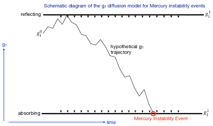
Figure 1: Schematic diagram of the $g_{1}$ diffusion model for Mercury instability events. $g_{1}$ is initialized at $g_{1}^{0}$ and diffuses. $g_{1}^{\uparrow}$ is a hard, reflecting upper boundary and $g_{1}^{\downarrow}$ is an absorbing lower boundary. If $g_{1}$ reaches $g_{1}^{\downarrow}$, a Mercury instability event occurs.

In this paper we will show that the $g_{1}$ diffusive model underpredicts the Mercury instability probability by a factor of 3–10,000 over the next 5 Gyr period in which the Sun will remain on the main sequence. We find that the discrepancy primarily results from the diffusive model producing variations of $g_{1}$ that are too small on timescales less than $\sim$0.3 Gyr. To better model the short-time variations of the $g_{1}$ trajectories, we propose a $g_{1}$ subdiffusive model (Fig. 2, and see Henry et al., 2010, for a review of subdiffusion). This is consistent with the work of Hoang et al. (2021), who found that $g_{1}$ subdiffuses by fitting a power law to the standard deviation of $g_{1}$ in a large ensemble of secular models as a function of time. Additionally, we find that a soft upper boundary on $g_{1}$, implemented as a quadratic spring potential above a certain value of $g_{1}$, provides a more accurate approximation of $N$-body model behavior than a hard, reflective upper boundary. We fit the parameters of our subdiffusive model to the short-time average tendency of $g_{1}$, mean square displacement of $g_{1}$, and probability density function (pdf) of $g_{1}$ from $N$-body simulations. This produces a six-parameter stochastic subdiffusive model that accurately reproduces $N$-body Mercury instability probabilities as small as $\sim$$10^{-4}$ (the lowest value we are able to estimate with $N$-body results due to limited sample size) and as high $\sim$0.5 (the highest value we are able to estimate with $N$-body results due to limited run lengths). The $g_{1}$ subdiffusive model is successful at reproducing a wide variety of statistics from the $N$-body code, suggesting that despite its simplicity, it captures important aspects of the relevant dynamics.

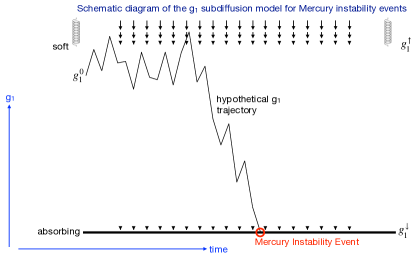
Figure 2: Schematic diagram of the $g_{1}$ subdiffusion model for Mercury instability events. $g_{1}$ is initialized at $g_{1}^{0}$ and subdiffuses. Note that the schematic subdiffusive $g_{1}$ trajectory is much more jagged, with larger movements on short timescales, than the schematic diffusive trajectory depicted in Fig. 1. $g_{1}^{\uparrow}$ is a soft upper boundary on $g_{1}$, implemented as a quadratic spring potential above a certain value of $g_{1}$. $g_{1}^{\downarrow}$ is an absorbing lower boundary. If $g_{1}$ reaches $g_{1}^{\downarrow}$, a Mercury instability event occurs.

2 Models

2.1 Model used to calculate $g_{1}$ statistics

We calculate $g_{1}$ statistics from the 2750 member Fix dt ensemble of simulations produced by Abbot et al. (2023). The simulations contain all 8 Solar System planets and no moons, asteroids, or comets. The simulations use the WHFAST integration scheme (Rein & Tamayo, 2015) from the REBOUND $N$-body code (Rein & Liu, 2012), which is a Wisdom-Holman scheme (WH) (Wisdom & Holman, 1991). The only parametrized physics scheme is an approximation of general relativity with a modified position-dependent potential (Nobili & Roxburgh, 1986), which is implemented as the gr_potential scheme in REBOUNDx (Tamayo et al., 2020). We initialized the simulations with Solar System conditions on February 10, 2018 taken from the NASA Horizons database and then added a uniform grid of perturbations to Mercury’s $x$-position, each separated by 10 cm. We used a fixed time step of $\sqrt{10}\approx 3.16$ days, which we demonstrated was sufficiently small to produce converged Mercury instability statistics (Abbot et al., 2023), and ran the simulations for 5 Gyr. The trajectories of eccentricity and $g_{1}$ are nearly identical among the simulations over the first 138 Myr of the simulation and then begin to noticeably separate from each other on the order of $\approx$1%. This is longer than the typical quoted value of $\sim$50 Myr for Solar System orbital calculations to diverge (e.g., Zeebe, 2017), possibly because Mercury’s eccentricity and $g_{1}$ may take longer to diverge than other variables.

The $g_{i}$ frequencies are defined through the following eigenfunction expansion (Murray & Dermott, 1999, Ch. 7):

$$e_{i}\cos\varpi_{i} =\sum_{k}M_{ik}\cos\alpha_{k},$$ (1)

$$e_{i}\sin\varpi_{i} =\sum_{k}M_{ik}\sin\alpha_{k},$$ (2)

where the index $i$ ranges over the planets $i=1,2,\ldots,8$, $e_{i}$ denotes the eccentricity of each planet, and $\varpi_{i}$ denotes the longitude of perihelion. The values $(M_{i,k})_{1\leq i,k\leq 8}$ are the coefficients in the eigenfunction expansion, and the terms $\alpha_{k}=g_{k}t+\beta_{k}$ describe the angles of the oscillations.

The first-order approximation with constant parameter values (1)-(2) is accurate over the shortest period of oscillation $\min_{i}2\pi/g_{i}$, but degrades thereafter. Indeed, when we fit the approximation to the output of a more complex $N$-body simulation, the values $M_{ik}$, $g_{k}$, and $\beta_{k}$ are all slowly changing as a function of time. Despite the imprecision, the first-order approximation leads to qualitative insights, as it correctly indicates the possibility for destabilization when two of the $g_{i}$ frequencies approach resonance.

To calculate $g_{1}$, we use the frequency_modified_fourier_transform routine (Šidlichovskỳ & Nesvornỳ, 1997) from the celmech package (Hadden & Tamayo, 2022), which requires a number of output times that is a power of 2. We find that $2^{10}$ output times are sufficient to obtain stable $g_{i}$ estimates from data, so we divide the Fix dt ensemble data into blocks of 10.24 Myr, with each block containing $2^{10}$ output times. Our calculated values of $g_{1}$ are therefore the average value over each 10.24 Myr segment. We apply frequency_modified_fourier_transform to $e_{1}\exp(i\varpi_{1})$ to calculate the four Fourier modes with the highest amplitude for a given 10.24 Myr segment and chose $g_{1}$ to be the $g_{i}$ closest to $g_{1}$ from the previous segment.

2.2 Model used to calculate 40 Gyr instability statistics

As a new contribution of this paper, we perform 1000 extensions of the Fix dt simulations. These extensions have exactly the same parameters as the Fix dt simulations described above, but we run them for a total of 40 Gyr. As in Abbot et al. (2021, 2023), we define a Mercury instability event as occurring when Mercury passes within 0.01 AU of Venus and stop the simulations at that point. In Abbot et al. (2023), we showed that after $10^{12}$ time steps (10 Gyrs), roundoff relative error is of order $10^{-5}$ for the semimajor axis and order $10^{-9}$ for the energy. Roundoff error is growing as $\sim t^{0.5}$ at 10 Gyr, so it should remain small for the 40 Gyr simulations we performed.

2.3 Ensemble of ensembles used to compute 5 Gyr instability statistics

To compute Mercury instability statistics on a timescale of less than 5 Gyr, we use the ensemble of $N$-body ensembles constructed by Abbot et al. (2023), which includes the 2501 member Laskar & Gastineau (2009) ensemble, the 1600 member Zeebe (2015a) ensemble, as well as both the 2750 member Var dt and 2750 member Fix dt ensembles of Abbot et al. (2023), for a total of 9601 members.

2.4 Diffusive and subdiffusive models

Both the diffusive and subdiffusive models are defined using fractional Brownian motion. Fractional Brownian motion is a mean-zero Gaussian process which we denote by $W(t)$ at each time $t\geq 0$. It is defined as the unique mean-zero Gaussian process which starts from $W(0)=0$ and has increments satisfying

$$\langle|W(t)-W(s)|^{2}\rangle=|t-s|^{2\alpha}$$ (3)

at all times $t,s\geq 0$. Here, $\alpha\in(0,1)$ is the Hurst parameter, which is $\alpha=1/2$ for a standard diffusion, whereas $\alpha\in(0,1/2)$ for a subdiffusion and $\alpha\in(1/2,1)$ for a superdiffusion (Henry et al., 2010, Sec. 1.2). As a result of the scaling relation (3), a subdiffusion exhibits larger variations over short timescales than a standard diffusion.

The simple diffusion model of Mogavero & Laskar (2021, Sec. 8.2) states that the $g_{1}$ value at time $t$ (units of Gyrs) is:

$$\tilde{g}_{1}(t)=g_{1}^{\uparrow}-|g_{1}^{0}+rW(t)-g_{1}^{\uparrow}|,$$ (4)

where $W(t)$ is a standard Brownian motion, $r>0$ is a scaling factor, $\tilde{g}_{1}(0)=g_{1}^{0}$ is the initial condition, and $g_{1}^{\uparrow}>g_{1}^{0}$ is a reflecting upper boundary condition. (We use the tilde notation to differentiate their simple diffusion model from our subdiffusion model.) As a result of (4), the probability density $\tilde{p}(g_{1},t)$ for $g_{1}$ at time $t$ evolves according to the Fokker-Planck equation (Gardiner, 2009, Ch. 5)

$$\partial_{t}\tilde{p}=\frac{r^{2}}{2}\partial^{2}_{g_{1}g_{1}}\tilde{p},\qquad g_{1}<g_{1}^{\uparrow},$$ (5)

with upper boundary condition

$$\left.\partial_{g_{1}}\tilde{p}\right|_{g_{1}=g_{1}^{\uparrow}}=0.$$ (6)

The process advances forward until hitting the lower boundary $g_{1}^{\downarrow}$ at a random time

$$\tilde{\tau}=\min\{t\geq 0:\tilde{g}_{1}(t)=g_{1}^{\downarrow}\}.$$ (7)

Then, instability occurs in the model (Fig. 1).

Mogavero & Laskar (2021, Sec. 8.2) motivate their use of a diffusion and reflecting upper boundary by observing that the pdf of $g_{1}$ has Gaussian tail behavior at low $g_{1}$ values, but drops off sharply at high $g_{1}$ values (Hoang et al., 2021). Woillez & Bouchet (2017) provide additional motivation, by referencing the theory of slow-fast dynamical systems (Gardiner, 2009, Ch. 6), in which the evolution of a slow variable can sometimes be modeled as a diffusive SDE. However, Hoang et al. (2021) argue that the time evolution of $g_{1}$ under the secular equations matches a subdiffusion more closely than a standard diffusion.

Next, we propose a more general model with two improvements: (1) We allow $W(t)$ to be a fractional Brownian motion with a Hurst parameter $\alpha$ not necessarily equal to $1/2$ and (2) we convert the reflecting boundary at $g_{1}^{\uparrow}$ into a soft upper boundary using a quadratic spring potential. In the general model, the $g_{1}$ value at time $t$ is given by the solution to the stochastic differential equation (SDE):

$$\mathop{dg_{1}}=-\partial_{g_{1}}H(g_{1})\mathop{dt}+r\mathop{dW},\qquad g_{1}(0)=g_{1}^{0},$$ (8)

where the potential energy term $H(g_{1})$ encodes the soft upper boundary:

$$H(g_{1})=\begin{cases}\frac{1}{2}k(g_{1}-g_{1}^{\uparrow})^{2},&g_{1}>g_{1}^{\uparrow}\\ 0,&g_{1}\leq g_{1}^{\uparrow}\end{cases}$$ (9)

This is the potential energy associated with a coiled spring. According to the model, $g_{1}(t)$ exhibits a negative tendency as soon as $g_{1}(t)>g_{1}^{\uparrow}$, with a magnitude proportional to a spring constant $k>0$. As the spring constant $k$ approaches infinity, the model converges to give a reflecting upper boundary. As a result of (8), the probability density $p(g_{1},t)$ evolves according to a Fokker-Planck equation (Ünal, 2007; Hahn et al., 2011)

$$\partial_{t}p=\partial_{g_{1}}(p\,\partial_{g_{1}}H(g_{1}))+\alpha r^{2}t^{2\alpha-1}\partial^{2}_{g_{1}g_{1}}p.$$ (10)

As before, the process advances forward until hitting the lower boundary $g_{1}^{\downarrow}$. Then, instability occurs.

Our fractional Brownian motion model is fundamentally different from the drift-diffusion model of Brown & Rein (2023), since we use a fractional Brownian motion in place of a Brownian motion. Additionally, our drift term $-\partial_{g_{1}}H(g_{1})$ is different from their drift term, since it depends only on $g_{1}$ and serves as a soft upper boundary. Here, the term “drift” refers to an instantaneous tendency and is common in the SDE literature (Gardiner, 2009). The drift term used by Brown & Rein (2023) depends only on time $t$ and changes the mean behavior of $g_{1}$, as they turn off general relativity in their model.

We use a forward Euler discretization to simulate from the diffusive and subdiffusive models. First, we use the algorithm of Dietrich & Newsam (1997) to generate a random vector containing the values of the fractional Brownian motion at discrete output times $\mathbf{W}=\bigl{(}W(\delta),W(2\delta),\ldots,W(N\delta)\bigr{)}$, as implemented in the stochastic package for python (Flynn, 2022). Next, we simulate from the simple diffusion model at the discrete output times $t=\delta,2\delta,\ldots,N\delta$ by setting

$$\tilde{g}_{1}(t)=g_{1}^{\uparrow}-|rW(t)+g_{1}^{0}-g_{1}^{\uparrow}|.$$ (11)

We simulate from our our subdiffusion model by setting $g_{1}(t=0)=g_{1}^{0}$ and applying the recursive update formula

$$g_{1}(t+\delta)-g_{1}(t)=-\delta\cdot\partial_{g_{1}}H(g_{1}(t))+r\bigl{[}W(t+\delta)-W(t)\bigr{]}.$$ (12)

At any time $t>0$, the discretization error when approximating $g_{1}(t)$ is guaranteed to vanish at a rate $\mathcal{O}(\delta^{1/2})$ or faster as $\delta\rightarrow 0$ (Butkovsky et al., 2021). We use $\delta=0.01$ Gyr, and confirm that our Mercury instability probability estimates have converged at this value.

parameters	Diffusive	Subdiffusive
$g_{1}^{0}$	$5.577\,^{\prime\prime}\,$yr-1	$5.65\,^{\prime\prime}\,$yr-1
$g_{1}^{\uparrow}$	$5.724\,^{\prime\prime}\,$yr-1	$5.85\,^{\prime\prime}\,$yr-1
$g_{1}^{\downarrow}$	$4.257\,^{\prime\prime}\,$yr-1	$4.9\,^{\prime\prime}\,$yr-1
$\alpha$	0.5	0.25
$r$	$0.197\,^{\prime\prime}\,$yr-1 Gyr-α	$0.16\,^{\prime\prime}\,$yr-1 Gyr-α
$k$	$\infty$	50 Gyr-1

Table 1: Parameters and their values for the diffusive and subdiffusive models. The parameter values for the diffusive model are taken from Mogavero & Laskar (2021), but rewritten using our variables.

3 Results

3.1 Problems with the $g_{1}$ diffusive model

In this subsection, we point out several issues with the $g_{1}$ diffusive model. As a starting point, the $g_{1}$ diffusive model is not effective at predicting Mercury instability probabilities over physically realistic timescales. On timescales longer than $\sim$10 Gyr, the model matches with the instability probabilities from secular model simulations (Mogavero & Laskar, 2021) and from our 40 Gyr $N$-body simulations (Fig. 3). However, on the 5 Gyr timescale of the future of the Solar System, the diffusive model underpredicts Mercury instability events by a factor of 3–1000 (Fig. 3).

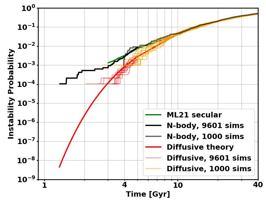
Figure 3: Probability that Mercury’s orbit becomes unstable as a function of time for the Mogavero & Laskar (2021) secular model (green), a 5 Gyr, 9601 member ensemble of the $N$-body model (black), a 40 Gyr, 1000 member ensemble of the $N$-body model (gray), the theoretical prediction of the diffusive model (red), ten 5 Gyr, 9601 member ensembles of stochastic realizations of the diffusive model (light red), and ten 40 Gyr, 1000 member ensembles of stochastic realizations of the diffusive model (orange). We obtained the Mogavero & Laskar (2021) results using a data digitizer.

One possible explanation for the fact that the $g_{1}$ diffusion produces too few Mercury instability events on shorter timescales ($<$10 Gyr) is that subdiffusion (Henry et al., 2010) better approximates the chaotic evolution of $g_{1}$. The main characteristic of subdiffusion is that it exhibits larger displacements on short timescales and smaller displacements on long timescales than diffusion. To investigate this idea quantitatively, we calculate the mean square displacement of $g_{1}$ ($\langle|\Delta g_{1}|^{2}\rangle$) across a range of time offsets ($\Delta t$) and consider a scaling relationship

$$\langle|\Delta g_{1}|^{2}\rangle\sim|\Delta t|^{2\alpha}$$ (13)

where $\alpha\in(0,1)$ is the Hurst parameter and can be chosen to match the data. As explained in section 2.4, $\alpha=1/2$ corresponds to standard diffusion, whereas $\alpha\in(0,1/2)$ corresponds to subdiffusion and $\alpha\in(1/2,1)$ corresponds to superdiffusion. Fig. 4(a) shows that $\alpha$ for the $N$-body model is much less than $1/2$ (we will show below that $\alpha\approx 0.25$), and the diffusive model produces a mean square displacement for $g_{1}$ that is too small on timescales less than $\sim$0.3 Gyr.

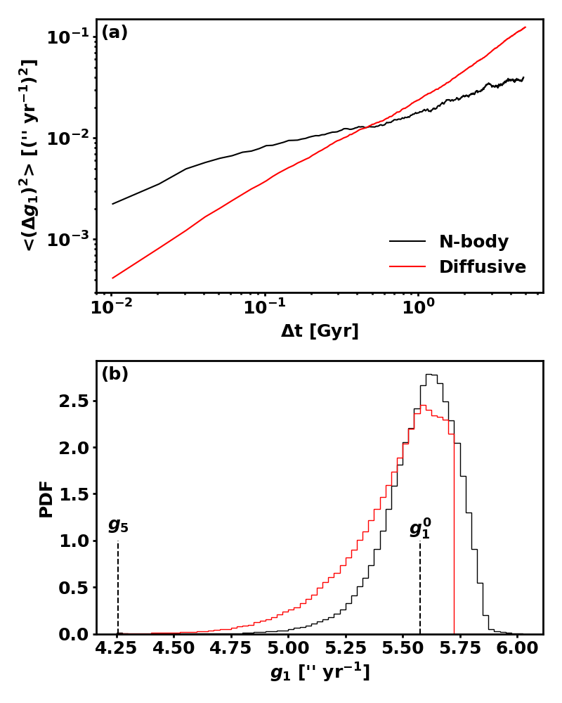
Figure 4: (a) Mean square displacement of $g_{1}$ as function of time offset ($\Delta t$) for the $N$-body model (black) and the diffusive model (red). (b) Probability distribution function of $g_{1}$ from the $N$-body model (black) and the diffusive model (red). The values of $g_{5}$ and $g_{1}^{0}$ are indicated on the plot.

Next, let us compare the pdf of $g_{1}$ between the $N$-body model and the diffusive model (Fig. 4(b)). The comparison immediately reveals that the upper boundary on $g_{1}$ in the $N$-body model is not hard. $g_{1}$ is not strictly limited to remain less than a particular value, although the probability density does drop off sharply which generates a skew (Hoang et al., 2021). It is also apparent that the diffusive model as tuned by Mogavero & Laskar (2021) overpredicts by an order of magnitude the probability that $g_{1}$ has a value less than 5$\,{}^{\prime\prime}\,$yr^-1. The unrealistic low values of $g_{1}$ occur in the diffusion model because the lower boundary on $g_{1}$ is set to be $g_{5}=4.257\,^{\prime\prime}\,$yr^-1. However, while the main physical mechanism for a Mercury instability event is a $g_{1}$-$g_{5}$ resonance (Batygin et al., 2015), the $g_{5}$ resonance might cause non-diffusive behavior as $g_{5}$ is approached. For example, the $g_{1}$ trajectories that lead to Mercury instability events in Figure 5 of Mogavero & Laskar (2021) often show large, erratic jumps from a value of $\sim 5\,^{\prime\prime}\,$yr^-1 to $g_{5}$ as the instability event occurs.

To conclude this subsection, the $g_{1}$ diffusive model has the following defects:

1. It underpredicts the Mercury instability probability on timescales less than 10 Gyr.

2. It produces too small variations in $g_{1}$ on timescales less than $\sim$0.3 Gyr.

3. It leads to a scaling of the mean square displacement $\langle|\Delta g_{1}|^{2}\rangle$ with the time offset $\Delta t$ that does not fit the $N$-body simulations.

4. Its hard, reflective upper boundary is not realistic.

5. It assumes that $g_{1}$ must diffuse all the way to $g_{5}$ to produce an instability event, which is not the case.

3.2 An improved $g_{1}$ subdiffusive model

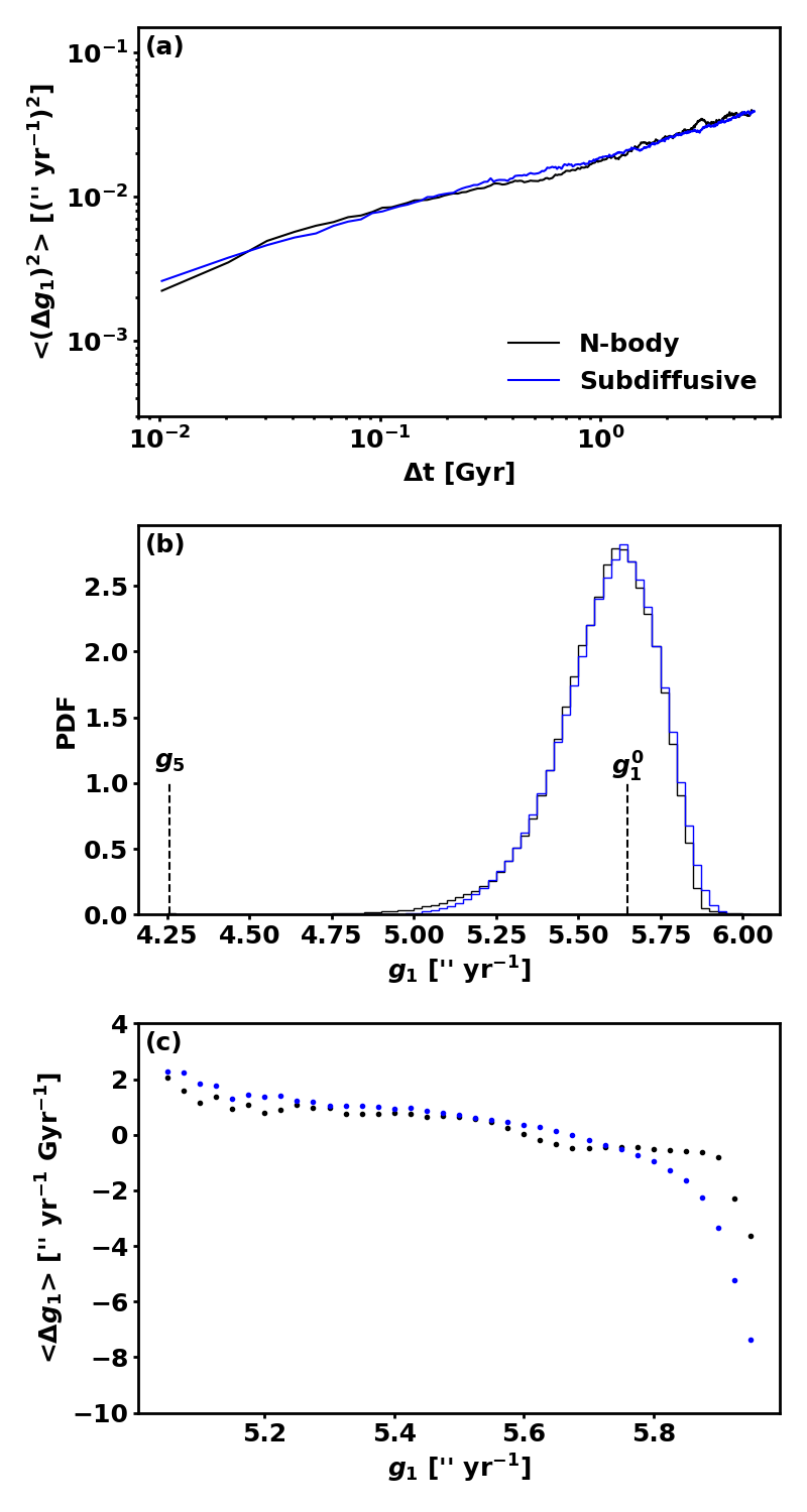
Figure 5: (a) Mean square displacement of $g_{1}$ as function of time offset ($\Delta t$) for the $N$-body model (black) and the subdiffusive model (blue). (b) Probability distribution function of $g_{1}$ from the $N$-body model (black) and the subdiffusive model (blue). The values of $g_{5}$ and $g_{1}^{0}$ are indicated on the plot. (c) Short-time drift $\langle\Delta g_{1}\rangle$ as a function of the starting value $g_{1}$ for the $N$-body model (black) and the subdiffusive model (blue). A time offset of 0.01024 Gyr was used to calculate the short-time drift of $g_{1}$.

We now apply our new subdiffusive model that addresses the limitations of the $g_{1}$ diffusive model. To begin, we impose the modeling assumption that the mean square displacement scales as a power law

$$\langle|\Delta g_{1}|^{2}\rangle=r^{2}|\Delta t|^{2\alpha}$$ (14)

over short timescales $\Delta t$. This modeling assumption fits the mean square displacement in the $N$-body data for $\alpha=0.25$ and $r=0.16\,^{\prime\prime}\,\text{yr}^{-1}$ (Fig. 5(a)). In comparison, Hoang et al. (2021) estimated $\alpha=0.26$ by fitting a power law to the standard deviation of $g_{1}$ in a large ensemble of secular models as a function of time.

Next, Fig. 5(c) shows that the $g_{1}$ trajectories from the $N$-body simulations exhibit an increasingly strong negative tendency over short-time intervals ($\Delta t=0.01\text{ Gyr}$) when $g_{1}$ exceeds a certain value $g_{1}^{\uparrow}$. We leave the interpretation of the drift to future work, but model it into the SDE (8) using the potential energy of a coiled spring, $H(g_{1})=\frac{1}{2}k\left(\max\{g_{1}-g_{1}^{\uparrow},0\}\right)^{2}$. We choose initial values of the upper boundary $g_{1}^{\uparrow}$ and the spring constant $k>0$ to match the short-time drift observed in the $N$-body simulations (Fig. 5(c)).

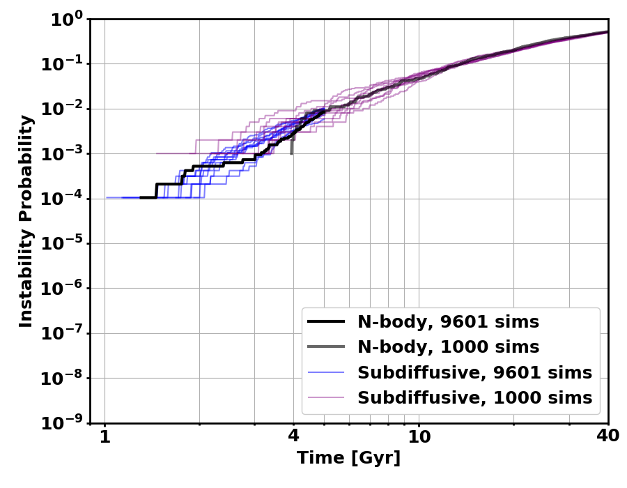
Figure 6: Probability that Mercury’s orbit becomes unstable as a function of time a 5 Gyr, 9601 member ensemble of the $N$-body model (black), a 40 Gyr, 1000 member ensemble of the $N$-body model (gray), ten 5 Gyr, 9601 member ensembles of stochastic realizations of the subdiffusive model (blue), and ten 40 Gyr, 1000 member ensembles of stochastic realizations of the subdiffusive model (purple). This figure should be compared with Fig. (3), which gives the equivalent information for the diffusive model.

After this, we choose $g_{1}^{0}$ so that the peak of the $N$-body and subdiffusive model pdfs match and the lower boundary $g_{1}^{\downarrow}$ so that only 1% of the $g_{1}$ values from the $N$-body simulations are less than $g_{1}^{\downarrow}$ (Fig. 5(b)). Finally, we fine-tune the value of $k$ on the order of 10% and $g_{1}^{\downarrow}$ on the order of 1% to improve the fit with the $N$-body model Mercury instability statistics (Fig. 6(a)).

The tuning procedure leads to the six parameters presented in Table 1. While we did not use an optimization algorithm to choose parameter values, we did systematically chose them to match the short-time and long-time behavior of the more complex $N$-body model. The purpose of this work is to show that the $g_{1}$ subdiffusive model produces a better approximation of the $N$-body model than the $g_{1}$ diffusive model, not to perfectly tune the subdiffusive model.

As the main result of our modeling efforts, the $g_{1}$ subdiffusive model yields an accurate approximation of the Mercury instability probability statistics for the $N$-body model both from 1–5 Gyr and from 5–40 Gyr (Fig. 6). The ability of the $g_{1}$ subdiffusive model to reproduce the Mercury instability statistics on timescales less than 10 Gyr is primarily due to larger variations in $g_{1}$ on timescales less than 0.3 Gyr and represents a significant advance beyond the previous $g_{1}$ diffusive model.

4 Discussion

The success of the $g_{1}$ subdiffusive model at approximating so many characteristics of the $N$-body model sets new challenges for the planetary dynamics community: First, why does $g_{1}$ subdiffuse rather than diffuse? Second, what is the physical cause of the restoring upper boundary on $g_{1}$ and why does it act as a coiled spring, rather than taking some other form? Given that the upper boundary prevents $g_{1}$ from resonating with $g_{2}\approx 7.45\,^{\prime\prime}\,$yr^-1, why isn’t there a restoring lower boundary on $g_{1}$ that prevents it from reaching $g_{5}$ and thereby prevents Mercury instability events?

Clues to the answers to these questions may lie in the properties of a conservative, Hamiltonian system. The phase space of such systems are generically comprised of a mixture of regular and chaotic trajectories. The dynamics of two degree-of-freedom Hamiltonian systems are equivalent to those of area-preserving maps via the construction of Poincarè return maps. The mixed phase space of two-dimensional area-preserving maps consists of elliptic periodic orbits surrounded by KAM curves that constitute “islands” embedded in a chaotic “sea” (e.g., Lichtenberg & Lieberman, 1992). The KAM curves of these regular islands form strict barriers for trajectories in the chaotic regime. The “stickiness” of the borders of these regular islands could lead to behavior that can effectively be described as subdiffusion, similar to how diffusion on fractal materials can lead to subdiffusion (Henry et al., 2010). In higher dimensions, the surviving KAM tori of regular trajectories would no longer impose strict topological constraints on the phase space accessible to chaotic orbits, but may still limit the range of excursions in a way that can be described by a soft, spring-like boundary. Of course this discussion is highly speculative, and more detailed research is needed to satisfactorily explain the dynamical properties of the Solar system we have identified in this paper.

The $g_{1}$ subdiffusive model is an improvement over the $g_{1}$ diffusive model, but it does not produce identical behavior to the $N$-body model. It is useful for improving understanding of the $N$-body model, not for replacing it. For example, the $N$-body trajectories show intermittency, transitioning from sustained quiescent periods to sustained active periods (Fig. 7). Periods of relative quiescence could be associated with proximity to islands of regularity. It is possible that we had to tune $k$ to be slightly higher than the $N$-body model $g_{1}$ tendency indicated (Fig. 5(c)) to compensate for this intermittant behavior in some way. Finally, the $g_{1}$ model has one more parameter than the $g_{1}$ diffusive model, $k$, and additionally allows $\alpha$ to be tuned rather than assumed to have a value of 1/2 (Table 1). It is therefore possible the improved ability to model Mercury instability statistics is due to additional model parameters, although this seems unlikely given that the parameters were fit to the short timescale properties of $g_{1}$ that the diffusive model is not able to capture.

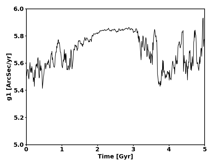
Figure 7: A sample trajectory of $g_{1}$ from the N-body model that demonstrates intermittency in behavior. Sustained quiescent periods alternate with sustained active periods.

The subdiffusive model fits Mercury instability statistics from the $N$-body model much better than the diffusive model on timescales less than 5 Gyr, but we do not have enough $N$-body Mercury instability events on timescales less than 2 Gyr to thoroughly test the subdiffusive model on the shortest timescales. One option would be to generate large enough ensembles (possibly with $10^{6}$ members) using a high-order secular code (e.g., Mogavero & Laskar, 2021) to estimate the probability of a Mercury instability event on these short timescales. Alternatively, more $N$-body Mercury instability examples on shorter timescales could be obtained using Diffusion Monte Carlo (Ragone et al., 2018; Webber et al., 2019; Ragone & Bouchet, 2021; Abbot et al., 2021) or action minimization (E et al., 2004; Plotkin et al., 2019; Woillez & Bouchet, 2020; Schorlepp et al., 2023) rare event schemes, aided by machine learning predictor functions (Ma & Dinner, 2005; Chattopadhyay et al., 2020; Finkel et al., 2021; Miloshevich et al., 2022; Finkel et al., 2023).

5 Conclusions

The main conclusions of this paper are:

1. The $g_{1}$ diffusive model underpredicts the Mercury instability probability relative to an $N$-body model by a factor of 3–10,000 on timescales less than 5 Gyr, which is the physically relevant timescale for the future of the Solar system. The underprediction results from the fact that the $g_{1}$ diffusive model produces too small variations of $g_{1}$ on timescales less than $\sim$0.3 Gyr.

2. We are able to fit $N$-body Mercury instability statistics on timescales of less than 5 Gyr as well as longer timescales using the $g_{1}$ subdiffusive model. We tune the model using short-time $g_{1}$ statistics including the $g_{1}$ probability distribution function, the time dependence of the $g_{1}$ mean square displacement, and the short-time drift of $g_{1}$.

3. We find that a soft upper boundary condition on $g_{1}$, parametrized as a quadratic spring potential, accurately approximates $N$-body behavior.

We thank Dan Fabrycky for extensive feedback on an early draft of this paper. This work was completed with resources provided by the University of Chicago Research Computing Center. D.S.A acknowledges support from NASA grant No. 80NSSC21K1718, which is part of the Habitable Worlds program. R.J.W. was supported by the Office of Naval Research through BRC Award No. N00014-18-1-2363 and the National Science Foundation through FRG Award No. 1952777, under the aegis of Joel A. Tropp. D.M.H acknowledges support from the CycloAstro project. J.W. acknowledges support from National Science Foundation through award DMS-2054306 and from the Advanced Scientific Computing Research Program within the DOE Office of Science through award DE-SC0020427. D.S.A. and J.W. acknowledge support from the Army Research Office, grant number W911NF-22-2-0124.


This research made use of the open-source projects Jupyter (Kluyver et al., 2016), iPython (Pérez & Granger, 2007), and matplotlib (Hunter, 2007).

References

- Abbot et al. (2023) Abbot, D. S., Hernandez, D. M., Hadden, S., et al. 2023, The Astrophysical Journal, 944, 190
- Abbot et al. (2021) Abbot, D. S., Webber, R. J., Hadden, S., Seligman, D., & Weare, J. 2021, The Astrophysical Journal, 923, 236
- Batygin & Laughlin (2008) Batygin, K., & Laughlin, G. 2008, The Astrophysical Journal, 683, 1207
- Batygin et al. (2015) Batygin, K., Morbidelli, A., & Holman, M. J. 2015, The Astrophysical Journal, 799, 120
- Boué et al. (2012) Boué, G., Laskar, J., & Farago, F. 2012, A&A, 548, A43, doi: 10.1051/0004-6361/201219991
- Brown & Rein (2020) Brown, G., & Rein, H. 2020, Research Notes of the AAS, 4, 221
- Brown & Rein (2022) —. 2022, Monthly Notices of the Royal Astronomical Society
- Brown & Rein (2023) —. 2023, Monthly Notices of the Royal Astronomical Society, 521, 4349
- Butkovsky et al. (2021) Butkovsky, O., Dareiotis, K., & Gerencsér, M. 2021, Probability theory and related fields, 181, 975, doi: 10.1007/s00440-021-01080-2
- Chattopadhyay et al. (2020) Chattopadhyay, A., Nabizadeh, E., & Hassanzadeh, P. 2020, Journal of Advances in Modeling Earth Systems, 12, e2019MS001958
- Dietrich & Newsam (1997) Dietrich, C. R., & Newsam, G. N. 1997, SIAM Journal on Scientific Computing, 18, 1088, doi: 10.1137/S1064827592240555
- E et al. (2004) E, W., Ren, W., & Vanden-Eijnden, E. 2004, Communications on Pure and Applied Mathematics, 57, 637, doi: https://doi.org/10.1002/cpa.20005
- Finkel et al. (2023) Finkel, J., Gerber, E. P., Abbot, D. S., & Weare, J. 2023, AGU Advances, 4, e2023AV000881
- Finkel et al. (2021) Finkel, J., Webber, R. J., Gerber, E. P., Abbot, D. S., & Weare, J. 2021, Monthly Weather Review, 149, 3647 , doi: 10.1175/MWR-D-21-0024.1
- Flynn (2022) Flynn, C. 2022, stochastic, https://stochastic.readthedocs.io/en/stable/, GitHub
- Gardiner (2009) Gardiner, C. 2009, Stochastic methods, Vol. 4 (Springer Berlin)
- Hadden & Tamayo (2022) Hadden, S., & Tamayo, D. 2022, The Astronomical Journal, 164, 179
- Hahn et al. (2011) Hahn, M. G., Kobayashi, K., & Umarov, S. 2011, Proceedings of the American Mathematical Society, 139, 691. http://www.jstor.org/stable/41059323
- Henry et al. (2010) Henry, B. I., Langlands, T. A., & Straka, P. 2010, in Complex Physical, Biophysical and Econophysical Systems (World Scientific), 37–89
- Hernandez et al. (2022) Hernandez, D. M., Zeebe, R. E., & Hadden, S. 2022, Monthly Notices of the Royal Astronomical Society, 510, 4302
- Hoang et al. (2021) Hoang, N. H., Mogavero, F., & Laskar, J. 2021, Astronomy & Astrophysics, 654, A156
- Hoang et al. (2022) —. 2022, Monthly Notices of the Royal Astronomical Society, 514, 1342
- Hunter (2007) Hunter, J. D. 2007, Computing in Science & Engineering, 9, 90, doi: 10.1109/MCSE.2007.55
- Kluyver et al. (2016) Kluyver, T., Ragan-Kelley, B., Pérez, F., et al. 2016, in Positioning and Power in Academic Publishing: Players, Agents and Agendas, ed. F. Loizides & B. Schmidt, IOS Press, 87 – 90
- Laskar (1994) Laskar, J. 1994, Astronomy and Astrophysics, 287, L9
- Laskar (2008) —. 2008, Icarus, 196, 1
- Laskar & Gastineau (2009) Laskar, J., & Gastineau, M. 2009, Nature, 459, 817
- Lichtenberg & Lieberman (1992) Lichtenberg, A., & Lieberman, M. 1992, Regular and Chaotic Dynamics
- Lithwick & Wu (2011) Lithwick, Y., & Wu, Y. 2011, ApJ, 739, 31, doi: 10.1088/0004-637X/739/1/31
- Lithwick & Wu (2014) Lithwick, Y., & Wu, Y. 2014, Proceedings of the National Academy of Sciences, 111, 12610
- Ma & Dinner (2005) Ma, A., & Dinner, A. R. 2005, The Journal of Physical Chemistry B, 109, 6769, doi: 10.1021/jp045546c
- Mackay et al. (1984) Mackay, R. S., Meiss, J. D., & Percival, I. C. 1984, Physica D Nonlinear Phenomena, 13, 55, doi: 10.1016/0167-2789(84)90270-7
- Meiss (1992) Meiss, J. D. 1992, Reviews of Modern Physics, 64, 795, doi: 10.1103/RevModPhys.64.795
- Meiss (2015) —. 2015, Chaos, 25, 097602, doi: 10.1063/1.4915831
- Miloshevich et al. (2022) Miloshevich, G., Cozian, B., Abry, P., Borgnat, P., & Bouchet, F. 2022, Probabilistic forecasts of extreme heatwaves using convolutional neural networks in a regime of lack of data, arXiv, doi: 10.48550/ARXIV.2208.00971
- Mogavero et al. (2023) Mogavero, F., Hoang, N. H., & Laskar, J. 2023, Physical Review X, 13, 021018
- Mogavero & Laskar (2021) Mogavero, F., & Laskar, J. 2021, arXiv e-prints, arXiv:2105.14976. https://arxiv.org/abs/2105.14976
- Mogavero & Laskar (2022) Mogavero, F., & Laskar, J. 2022, Astronomy & Astrophysics, 662, L3
- Murray & Dermott (1999) Murray, C. D., & Dermott, S. F. 1999, Solar system dynamics (Cambridge university press)
- Nobili & Roxburgh (1986) Nobili, A. M., & Roxburgh, I. W. 1986, in Symposium-International astronomical union, Vol. 114, Cambridge University Press, 105–111
- Pérez & Granger (2007) Pérez, F., & Granger, B. E. 2007, Computing in Science and Engineering, 9, 21, doi: 10.1109/MCSE.2007.53
- Plotkin et al. (2019) Plotkin, D. A., Webber, R. J., O’Neill, M. E., Weare, J., & Abbot, D. S. 2019, Journal of Advances in Modeling Earth Systems, 11, 863
- Ragone & Bouchet (2021) Ragone, F., & Bouchet, F. 2021, Geophysical Research Letters, 48, e2020GL091197
- Ragone et al. (2018) Ragone, F., Wouters, J., & Bouchet, F. 2018, Proceedings of the National Academy of Sciences, 115, 24, doi: 10.1073/pnas.1712645115
- Rein & Liu (2012) Rein, H., & Liu, S.-F. 2012, Astronomy & Astrophysics, 537, A128
- Rein & Tamayo (2015) Rein, H., & Tamayo, D. 2015, Monthly Notices of the Royal Astronomical Society, 452, 376
- Schorlepp et al. (2023) Schorlepp, T., Tong, S., Grafke, T., & Stadler, G. 2023, Scalable Methods for Computing Sharp Extreme Event Probabilities in Infinite-Dimensional Stochastic Systems. https://arxiv.org/abs/2303.11919
- Šidlichovskỳ & Nesvornỳ (1997) Šidlichovskỳ, M., & Nesvornỳ, D. 1997, in The Dynamical Behaviour of our Planetary System: Proceedings of the Fourth Alexander von Humboldt Colloquium on Celestial Mechanics, Springer, 137–148
- Tamayo et al. (2020) Tamayo, D., Rein, H., Shi, P., & Hernandez, D. M. 2020, MNRAS, 491, 2885, doi: 10.1093/mnras/stz2870
- Webber et al. (2019) Webber, R. J., Plotkin, D. A., O’Neill, M. E., Abbot, D. S., & Weare, J. 2019, Chaos: An Interdisciplinary Journal of Nonlinear Science, 29, 053109
- Wisdom & Holman (1991) Wisdom, J., & Holman, M. 1991, AJ, 102, 1528, doi: 10.1086/115978
- Woillez & Bouchet (2017) Woillez, E., & Bouchet, F. 2017, Astronomy & Astrophysics, 607, A62
- Woillez & Bouchet (2020) —. 2020, Physical Review Letters, 125, 021101
- Zaslavsky (2002) Zaslavsky, G. 2002, Physics Reports, 371, 461, doi: 10.1016/S0370-1573(02)00331-9
- Zeebe (2015a) Zeebe, R. E. 2015a, The Astrophysical Journal, 811, 9
- Zeebe (2015b) —. 2015b, The Astrophysical Journal, 798, 8
- Zeebe (2017) —. 2017, The Astronomical Journal, 154, 193
- Ünal (2007) Ünal, G. 2007, in Mathematical Physics - Proceedings of the 12th Regional Conference, 53–60, doi: 10.1142/9789812770523_0008