Critical properties of the optical field localization in a three-dimensional percolating system: Theory and experiment

Abstract

We systematically study the optical field localization in an active three-dimensional (3D) disordered percolating system with light nanoemitters incorporated in percolating clusters. An essential feature of such a hybrid medium is that the clusters are combined into a fractal radiation pattern, in which light is simultaneously emitted and scattered by the disordered structures. Theoretical considerations, based on systematic 3D simulations, reveal nontrivial dynamics in the form of propagation of localized field bunches in the percolating material. We obtain the length of the field localization and dynamical properties of such states as functions of the occupation probability of the disordered clusters. A transition between the dynamical states and narrow point-like fields pinned to the emitters is found. The theoretical analysis of the fractal field properties is followed by an experimental study of the light generation by nanoemitters incorporated in the percolating clusters. The experimental results corroborate theoretical predictions.

I Introduction

Disordered photonic materials can transmit and trap light through random multiple scattering that leads to formation of electromagnetic modes depending on the structural correlations, scattering strength, and dimensionality of the system Riboli:2014 ; Vynck:2012 ; Flach:2009 ; Sheng:2010 ; Wang:2011 ; Jendrzejewski:2012 ; Segev:2013a ; Wiersma:2013a ; Matis:2022 ; Skipetrov:2018 ; Cobus:2018 . The Anderson localization was predicted as a non-interacting linear interference effect Anderson:1958 . However, in real systems non-negligible interaction between light and medium takes place. Therefore, an important aspect of the optical localization is the interplay between nonlinear self-interaction of light in the disordered medium and the linear Anderson effect in the same medium Segev:2013a . The linear localization of classical waves can be interpreted as a result of interference between their amplitudes associated with scattering paths of wave packets propagating among the diffusers. The study of field transitions in three-dimensional (3D) disordered optical systems has not yet led to fully established conclusions, in spite of considerable efforts. The localization transition may be difficult to reach for the light waves due to the action of various detrimental effects in dense disordered media required to achieve strong scattering (see Ref. Skipetrov:2016a and references therein). The experimental observation of optical Anderson localization Faez:2009a just below the field transition in a 3D disordered medium shows strong fluctuations of the wave function that leads to nontrivial length-scale dependence of the intensity distribution (multifractality). To study the field localization in disordered systems, one randomly perturbs parameters (for instance, the refractive index) around a mean value, and then identifies guided modes in such a disordered medium, see, e.g., Ref. karbasi:2012 and references therein. It is often assumed that materials have well-defined mean values of local coefficients, that do not lead to critical behavior.

Other physically relevant random media are percolating systems, where the disorder is defined by a value of population probability $p$. A fundamental feature of such a system is that, in a vicinity of the critical (threshold) value, $p=p_{\mathrm{cr}}$, the percolation phase transition occurs. It leads to the formation of long-range connectivity on a scale determined by the system’s length or the size of a spreading percolating cluster. The spreading cluster has a disordered shape, that essentially affects properties of the medium Stauffer:2003 . The resulting disordered structure is characterized by a non-integer fractal dimension $D_{F}$.

In this work, we aim to study the localization of an optical field in the 3D percolating disorder, with percolating clusters filled by light nanoemitters in the excited state. The peculiarity of the setup is that in such materials the clusters create a fractal nonlinear radiating system where light is both emitted and scattered by inhomogeneity of the clusters. Such a system may be considered as a 3D extension of the localization mechanism acting in a one-dimensional waveguide in the presence of controlled disorder Billy:2008a . In 3D disordered percolating systems, the optical transport was observed Burlak:2009a , and it was also found that random lasing, assisted by nanoemitters incorporated in such a disordered structure, can occur Burlak:2015 .

The linear theory of the field localization in such a system, that is valid for very small times (smaller than the laser generation time) was developed in Ref. Burlak:2017 . However the consideration of small times does not make it possible to study nonlinear dynamical effects that emerge on a longer time scale, close to the lasing threshold in such a system. Then, the following issues are relevant in this context: (i) the onset of the optical-field localization in a 3D active time-irreversible nonlinear system, cf. Ref. Sheng:2010 , and (ii) the existence of a transition separating localized propagating optical states and static fields pinned to random radiating emitters.

The rest of the paper is organized as follows. In Section II we formulate the model. Section III reports numerical results concerning the lasing by nanoemitters in the percolating medium. In Section IV we discuss the optical localization, while in Section V we study the transition separating the propagating states and narrow field patterns pinned to the emitters. In Section VI we report results of our experimental investigation of the light generation by nanoemitters incorporated in the percolating cluster. The last Section concludes the paper.

II Basic equations

The percolation normally refers to the leakage of fluid or gas through porous materials. We consider the setting in which percolating clusters are filled by nanoemitters in an excited state. A typical incipient percolation cluster has a dendrite shape, see Fig. 1. In Fig. 1 we observe that such a system exhibits two essentially different domains. The first one (close to the entrance shown by the arrow) features strong concentration of percolation clusters, which may lead to enhancement of nonlinear field effects and commencement of lasing. In the other domain, the concentration is small, hence the local disorder strength of the medium is small too.

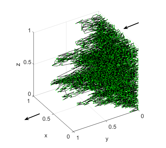
Figure 1: (Color online) A typical spatial structure of the incipient percolating cluster near the percolation threshold at $p=0.3$ in the cube of size $l_{0}{\times}l_{0}{\times}l_{0}$, with $l_{0}=10^{-4}~{}m$. To display necessary details, a numerical grid of size $100{\times}100{\times}100$ is used in this figure. Only spanning clusters are shown, while internal ones detached from the entry plane are not displayed. In this configuration, a considerable number of emitters are incorporated close to the entry (indicated by the incoming arrow). Solid lines (green color) connect nodes linked by the variational Fermat’s principle, see details in Ref. Burlak:2015 .

In what follows we address the lasing by nanoemitters incorporated in a spanning percolating cluster that occupies a large portion of the working space. First it is instructive to display the 3D spatial structure of the incipient cluster for the population probability $p$ taking values nearly the percolation transition. Figure 1 exhibits such a cluster (all internal disconnected clusters are omitted) for $0.3\leq p\leq p_{\mathrm{cr}}\approx 0.318$. The figure displays a fractal structure of the incipient cluster, similar to that produced in Ref. Burlak:2015 . The cluster features a dendrite shape that depends on the actual random sampling. Re-running simulations with another random seed will lead to a percolation cluster with a different dendrite structure.

III Lasing by nanoemitters

As mentioned above, we assume that the percolating clusters with the dendrite shape are filled by light nanoemitters in the excited state. The Maxwell’s equations for electric $\mathbf{E=E(r,t)}$ and magnetic $\mathbf{H=H(r,t)}$ fields in the system are

$$\nabla\times\mathbf{E}=-\mu_{0}\frac{\partial\mathbf{H}}{\partial t}\text{, }\nabla\times\mathbf{H}=\varepsilon\frac{\partial\mathbf{E}}{\partial t}+\sum_{k}\mathbf{j}(\mathbf{R}_{k},t)\delta_{\mathbf{rR}_{k}}\text{{, } }$$ (1)

where $\mathbf{j}(\mathbf{R}_{k},t)$ ($k=1,..,M$) is the electric current in radiating emitters set at positions $\mathbf{R}_{k}$. The equation for the polarization density $\mathbf{P}_{k}\mathbf{\equiv P(\mathbf{R}_{k},}t\mathbf{)}$ in the cluster filled by the emitters (four-level atoms), with level occupations $N_{m,k}$ ($m=0,1,2,3$ is the level’s number), is

$$\frac{\partial^{2}\mathbf{P}_{k}}{\partial t^{2}}+\Delta\omega_{a}\frac{\partial\mathbf{P}_{k}}{\partial t}+{\omega_{a}^{2}}\mathbf{P}_{k}=\frac{6\pi\varepsilon_{0}c^{3}}{\tau_{21}\omega_{a}^{2}}(N_{1,k}-N_{2,k})\mathbf{E}_{k}.\text{ }$$ (2)

To complete the model we add the rate equations for the level occupations of emitters, $N_{i,k}=N_{i}(\mathbf{\mathbf{R}_{k}},t)$:

$$\frac{\partial N_{0,k}}{\partial t}=-A_{r}N_{0,k}+\frac{N_{1,k}}{\tau_{13}}\text{, }\frac{\partial N_{3,k}}{\partial t}=A_{r}N_{0,k}-\frac{N_{3,k}}{\tau_{02}},$$ (3)

$$\frac{\partial N_{1,k}}{\partial t}=\frac{N_{2,k}(t)}{\tau_{(21),(32)}}-\frac{(\mathbf{j}\cdot\mathbf{E})_{k}}{\hbar\omega_{a}}-\frac{N_{1,k}}{\tau_{13}}\text{, }\frac{\partial N_{2,k}}{\partial t}=\frac{N_{1,k}(t)}{\tau_{12}}+\frac{(\mathbf{j}\cdot\mathbf{E})_{k}}{\hbar\omega_{a}}-\frac{N_{2,k}}{\tau_{02}}\text{,}$$ (4)

Here $\Delta\omega_{a}=\tau_{21}^{-1}+2T_{2}^{-1}$, where $T_{2}$ is the mean time between dephasing events, $\tau_{21}$ is the time of the spontaneous decay from the second atomic level to the first one, and $\omega_{a}$ is the radiation frequency (see, e.g., Siegman:1986 ). Electric field $\mathbf{E(r,}t\mathbf{)}$ and current $\mathbf{j(\mathbf{R}_{k},}t\mathbf{)}=\partial\mathbf{P(\mathbf{R}_{k},}t\mathbf{)}/\partial t$ are found from the Maxwell’s equations, together with equations for densities $N_{m}\mathbf{(\mathbf{R}_{k},}t\mathbf{)}$ of atoms residing at the $m$-th level. An external source excites the emitters from the ground level ($m=0$) to the third level at certain rate $A_{r}$, which is proportional to the pumping intensity Soukoulis:2000 . After a short lifetime $\tau_{32}$, the emitters transfer nonradiatively to the second level. The second and first levels are the top and bottom lasing levels, respectively. Emitters decay from the top level to the bottom one through spontaneous or stimulated emission, $(\mathbf{j}\cdot\mathbf{E})/\hbar\omega_{a}$ being the stimulated-radiation rate. Finally, emitters can also decay nonradiatively from the first level to the ground level. The lifetimes and energies of the top and bottom lasing levels are $\tau_{21}$, $E_{2}$ and $\tau_{10}$, $E_{1}$, respectively. The individual radiation frequency of each emitter is then $\omega_{a}=\left(E_{2}-E_{1}\right)/\hbar$.

To study the dynamics, we solved the semiclassical equations (1) - (4) that couple field $\mathbf{E(r,t)}$, polarization density $\mathbf{P(\mathbf{R}_{k},}t\mathbf{)}$, and occupations of the emitters’ levels $N_{i}\mathbf{(\mathbf{R}_{k},}t\mathbf{)}$. In the following Section we use the numerical finite-difference time-domain algorithm FDTD implemented on the numerical grid of size $100\times 100\times 100$ to produce 3D solutions to Eqs. (1)-(4). The solutions are presented in terms of scaled time $t$ and coordinates $\mathbf{r}$ defined by $t\rightarrow{tc}_{0}{/l_{0}}$ and $\mathbf{r}\rightarrow\mathbf{r}{/l_{0}}$, where

$$l_{0}=23.0~{}\mathrm{\mu}\text{{m}}$$ (5)

is a typical spatial scale (corresponding to our experimental setup, see below), and $c_{0}$ is the light speed in vacuum.

We aim to calculate the time-averaged integral emission of electromagnetic energy from a cubic sample $(x,y,z)\in[0,l_{0}]$. The total output flux of energy can be written as

$$I=\oint_{S}(\mathbf{K}\cdot\mathbf{n})dS=I_{x}+I_{y}+I_{z},$$ (6)

where $\mathbf{K}$ is the time averaged Pointing vector, $\mathbf{n}$ is the normal unit vector on surface $S$ of cube, and $I_{x,y,z}$ are energy fluxes (intensities) emitted from both faces of the cube perpendicular to a particular direction. To calculate the energy flux defined by Eq. (6), we solved numerically the equations that couple polarization density $\mathbf{P}$, electric field $\mathbf{E}$, and four-level occupations of the emitters.

Figure 2 shows the evolution of the field energy fluxes $I_{x,y,z}$ on the output surface of the sample. In panel 2(a) we observe that initial field amplitudes are very small, so that the system of Eqs. (1)-(4) is effectively linear at the initial stage of the evolution.

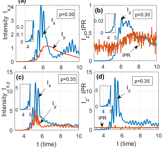
Figure 2: (Color online) The lasing output (stimulated by the nanoemitters embedded in the percolating clusters) with intensities (arb.units) (a) $I_{x,y}$, (b) $I_{z}$ [defined by Eq. (6)], and the inverse participation ratio (IPR), defined as per Eq. (7), as functions of time $t$. In (a,b) the percolating probability is $p=0.30$, while in (c,b) it is $p=0.35$. Insets in panels (a)-(d) display the initial evolution of intensities $I_{x},I_{z}$ at small times $t<5$ (for respective values $p$), from which one observes that lasing starts at time $t_{C}\approx 4.1$, and then exponentially rapidly approaches the peak values at $t\approx 4.8$. After that, the nonlinear dynamics commences.

At times $t<t_{C}\approx 4.1$ synchronization of initially random phases of the emitters in the clusters occurs. Then, at times close to $t=t_{C}$, Fig. 2 demonstrates the generation of a strong field output that corresponds to the onset of lasing in the ensemble of excited emitters embedded in the clusters. Insets in Figs. 2(a-d) display the initial dynamics of intensities $I_{x,y}$ and $I_{z}$ at $t<5$ (for the respective values of the percolation probability, $p=0.30$ and $0.35$), showing that the lasing starts at time $t_{C}\approx 4.1$ and then it exponentially rapidly attains peak values at time $t\approx 4.8$, at which the nonlinear dynamics commences. Starting from $t=t_{C}$, the disordered percolating system features the transition to the optical generation, when, in addition to the amplification, the optical waves undergo multiple scattering in the percolating fractal medium. As the lasing starts in all field modes, the optical field and radiating nanoemitters form a strongly coupled nonlinear dynamical system. To evaluate the strength of the field distribution, we calculated the inverse participation ratio (IPR) of the field, defined as

$$IPR=\frac{l_{0}^{3}\int\left|\mathbf{E}\right|^{4}d^{3}\mathbf{r}}{\left(\int\left|\mathbf{E}\right|^{2}d^{3}\mathbf{r}\right)^{2}},$$ (7)

where $l_{0}$ is the sample’s size, and the integration is performed over the entire system. Figure 2(b) demonstrates complex oscillatory behavior of IPR, which implies a high degree of randomicity in the system. However, after the onset of the lasing, IPR as a whole exhibits a trend to transition towards a more ordered state of the field. The dynamics of the population of the four levels of the nanoemitters, which follows the phase synchronization and the onset of the lasing, is displayed in Fig. 3. In particular, the evolution of populations $N_{1,2}$ that leads to the start of the lasing is shown in Fig. 3(b).

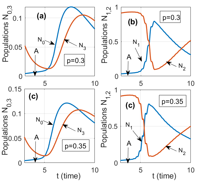
Figure 3: (Color online) The evolution of populations $N_{j}$ ($j=0,1,2,3$) of the four levels in the radiating nanoemitters incorporated in the percolating clusters: (a) $N_{0,3}$ and (b) $N_{1,2}$ vs. time $t$. In (a,b) the percolating probability is $p=0.30$, and in (c,b) it is $p=0.35$. Vertical arrows $\mathrm{A}$ indicate the critical time, $t_{C}\approx 4.1$, at which the lasing starts, cf. Fig. 2. The nonlinear dynamics commences at $t>t_{C}$.

IV The localization

Random multiple scattering of optical waves leads to field localization, in the form of well-trapped modes. Such states are defined by a characteristic average localization radius of the optical field. If the field amplitude in the localized mode is small, it propagates as a free one in the linear regime.

As this phenomenon occurs in the highly disordered system, it may be identified as a variant of the 3D optical-field localization. Similar to the widely adopted approach in the field localization theory, see Ref. Genack:2010 and references therein, we define the dimensionless localization measure, $g$, as the ratio of two spatial scales: the mean free paths of photons in a sample, $\bar{l}$, and wavelength $\lambda$ of the radiation of emitters embedded in the percolating cluster. Length $\bar{l}$ is proportional to the (dimensionless) distance $A_{\mathrm{3D}}$ which is a number of nodes in the numerical grid, which a photon can travel in the 3D sample, passing $N_{e}(p)$ emitters without visiting the same region twice. $A_{\mathrm{3D}}$ is calculated directly in our simulations by dint of the TSP (Traveling Salesman Problem) technique Press:2002 . Accordingly, the dimensionless average free path is $A_{\mathrm{3D}}/N_{e}(p)$, its dimensional counterpart being $\bar{l}=l_{0}A_{\mathrm{3D}}/N_{e}$, where $l_{0}$ is the basic length scale (5) defined above. Thus, the localization measure is

$$g(p)=\frac{l_{0}}{\lambda}\frac{A_{3N}}{N_{e}(p)}.$$ (8)

For the percolating grid considered here, the numerically computed dependence $g(p)$ is presented in Fig. 4 for typical values of physical parameters: $l_{0}=23~{}\mathrm{\mu}$m, $\lambda=0.5~{}\mathrm{\mu}$m.

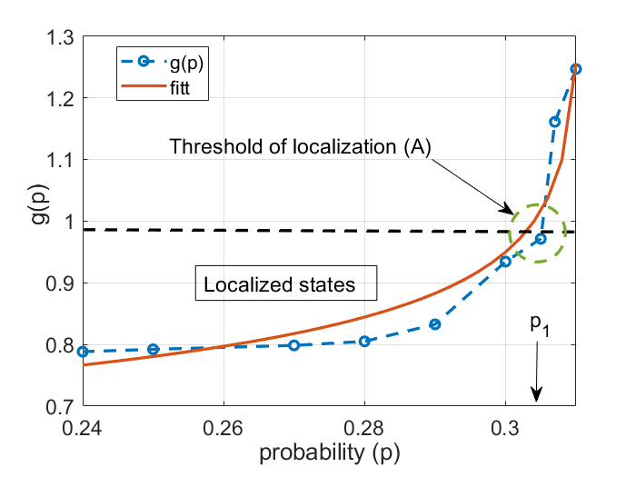
Figure 4: (Color online.) Dependence $g(p)$, as produced by numerical solution of Eq. (8) (blue dash line) for typical values of physical parameters: field wavelength $\lambda=0.5~{}\mathrm{\mu}$m and scale length $l_{0}=23~{}\mathrm{\mu}$m. The red line is the analytical fitting by the probe function $g_{f}(p)=b+|p-a|^{m}$ that gives $a=0.31,m=-0.074$, which turns out to be close to critical percolation $p_{c}$ and critical exponent $\nu$ respectively, and $b=-0.45$. The Ioffe-Regel localization condition, $g\approx 1$, is fulfilled closely of the percolation threshold, $p\approx p_{c}=0.318$. Large values of $p$ produce very long free paths $A_{\mathrm{3D}}$, corresponding to $g>1$, where the localization does not occur. The region of $g(p)<1$ is indicated as one maintaining localized states. Arrow A indicates the area of the localization threshold, which is $3.01<p<3.1$. The exact value of probability $p$ corresponding to the point $g(p)=1$ is calculated from $g_{f}(p)=1$, that gives $p_{1}=0.304$. It is difficult to obtain more precise values because of the enhacement of fluctuations in the area of the percolation phase transition at $p\approx p_{c}$ Stauffer:2003 .

The Ioffe-Regel localization condition, $g=1$ Ioffe ; Sheng:2010 , takes place close to the percolation threshold, $p$ $\approx 0.318$, indicated by arrow (A) in Fig. 4. Further increase of $p$ leads to larger values of the above-mentioned dimensionless distance $A_{\mathrm{3D}}$, hence the localization does not occur at $g>1$, while it persists at $g(p)<1$. It is difficult to calculate a precise value of probability $p$ corresponding to the point $g(p)=1$ because of significant increase of fluctuation in the area of the percolation phase transition at $p\approx p_{c}$ Stauffer:2003 .

Generally, the structure of the radiated field in the 3D percolating medium is quite intricate, see Fig. 5, which displays the isosurface of the 3D emitted field at time $t=11$. We observe an indented shape of light structures with bunches and wormholes due to the fractality of the radiating system.

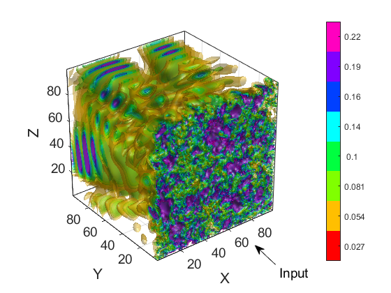
Figure 5: (Color online.) The 3D isosurface of the emitted field at time $t=11$ for $p=30$. The fractality of the field gives rise to the complex structure with “wormholes” and field bunches.

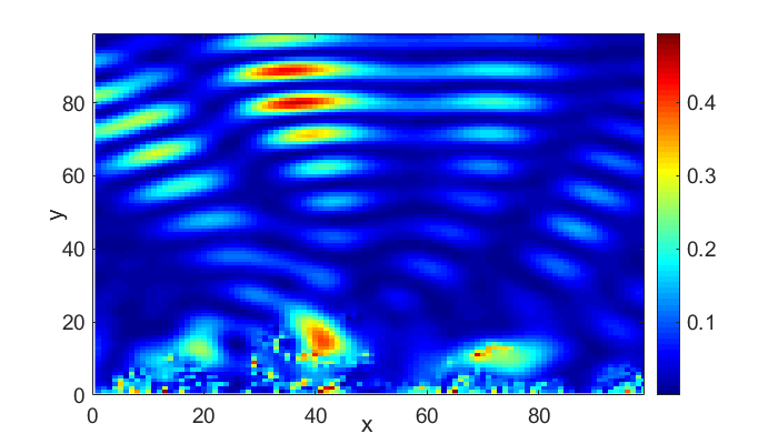
Figure 6: (Color online) The normalized field (arb.units) in the midplane $\left(x,y\right)$ of the 3D system, corresponding to Fig. 5 at $z=L/2$ for $p=0.3$. In the input area (small $y$), only narrow point-like fields generated by static random emitters are observed. Farther, field bunches with a smooth localized shape and large amplitudes arise beyond the emitter’s peaks. Thus, lasing in the percolating disordered system stimulates the localization of the emitted field.

Figure 5 demonstrates the screenshot of the system after some transition time $t=11$ (see the field peaks in Fig. 3), when dynamics becomes nonlinear. The field peaks detach from the emitters and generate 3D field bunches in the course of the evolution. In what follows below, we address the dynamics and structure of the localized fields confined in the light bunches. A quasi-spherical field bunch is referred to as a bounded 3D domain, schematically separated into concentric spherical layers numbered from the center to periphery by numbers $j$, with field $\left|E_{j}\right|$ being a decreasing function of $j$, i.e., $\left|E_{0}\right|>\left|E_{1}\right|>\ldots>\left|E_{r}\right|>0$, where $r$ is the number (effectively, radius) of the concentric layers. Each bunch is characterized by two parameters, viz., radius $r$ and the value of the field at the center, $\left|E_{0}\right|=E_{\max}$ (a more precise consideration of such a 3D localization problem requires the use of huge computational resources). One of these bunches is shown in Fig. 7, where one can clearly observe the structure of the localized field with a large amplitude $E_{\max}$ and characteristic radius $r$ at time $t=11$. We have found that such well-established localized objects are generated at various locations in the 3D medium due to disordered positions of the radiating emitters and the fractal shape of the percolating clusters. Fig.6 exhibits the normalized field (arb.units) in the midplane $\left(x,y\right)$ of the 3D system, corresponding to Fig. 5 at $z=L/2$ for $p=0.3$. In the region of irregular point-like emitters (small y in Fig.6) the strong (nonlinear) fields are generated dynamically with reproducing the localized shape of the emitter clusters. This leads to the following: the field pulses bounce off the emitters and then propagate independently in the form of inhomogeneous (smooth) waves. The spatial localization of such pulses (in a transversal plane) can be seen in Fig. 6. The localized bunches propagate from the emitters positions and thereafter arrive the output boundaries, where they are observed as the temporal field peaks, see Fig. 2. Fig. 5 displays the details of such a dynamics in 3D.

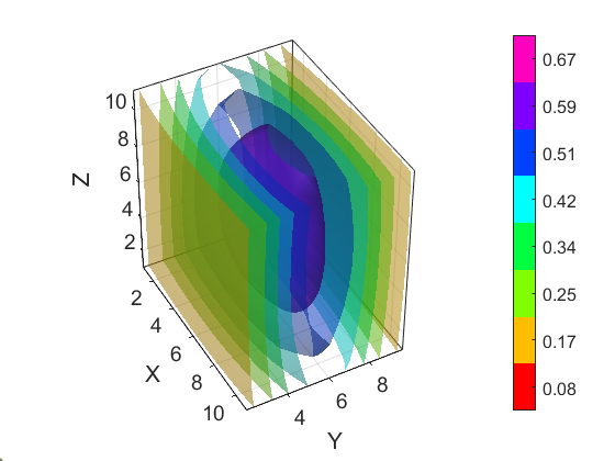
Figure 7: (Color online) The shape of a localized field bunch, with a high field amplitude at the center, $E_{\max}=0.98$, and radius $r=5$ at $t=11$, for $p=0.3$,. The center of the structure is located at the point with coordinates $\left\{x=14,y=18,z=73\right\}$. In the general case, the localized bunches are centered at random positions.

V The transition to the localization

Due to the statistical nature of the field localization, our approach here is based on multiple realizations of the disordered percolating structure, sampled over a statistically identical ensemble of the emitters. In active media (where the time reversibility is broken), such an approach has to develop the description of the localization strength in terms of the time-average states. In this case, the percolating population probability of the host material becomes the control parameter that allows one to distinguish localized and extended modes.

Because of the inhomogeneity of the distribution of the disordered emitters and fractal shape of the percolating clusters, the radiated field acquires an essentially non-uniform shape featuring the above-mentioned dynamical bunches. Therefore, in what follows below, we consider percolation probability $p$ as the parameter which determines the average radius of the bunches. A region where such a radius is a persistent feature is identified as the localization domain. Localization-transition zones are defined as regions where the localization radius changes sharply. It is worth noting that the velocity of the dynamical optical bunches can be well established only beyond the area of the active emitters, as in that area the propagating field is coupled to the light emitters and thus cannot be separated from the narrow point-like field of the static nanoemitters.

In what follows we study the dependence of the number of bunches $M$ at different times $t$ on radius $r$, for a fixed percolation probability, $p=0.3$, which is slightly smaller than the above-mentioned threshold value, $p_{\mathrm{cr}}=0.318$ Stauffer:2003 , Wang:2013a Figure 8 shows such a dependence for scaled times $t=1,...,19$. It is observed that, below the lasing threshold ($t\leq 5$, see Fig. 6), there are many field peaks with small radius $r$. Most of them correspond to narrow point-like field packets generated by the static randomly distributed light emitters, cf. Fig. 6. However, Fig. 8 demonstrates that, after the lasing starts (at $t>5$), the number of the optical bunches with large radius $r$ drastically increases. Besides, Fig. 6 shows that such bunches (with large $r$) are situated mainly beyond the percolation area. Moreover, as the same figure shows, the bunches feature a well-defined shape; they are no longer pinned to the static emitters, migrating to the region where emitters are not present. These features allow one to identify such dynamical bunches as 3D zones of the nonlinear optical-field localization emerging in the active percolating clusters with the fractal structure.

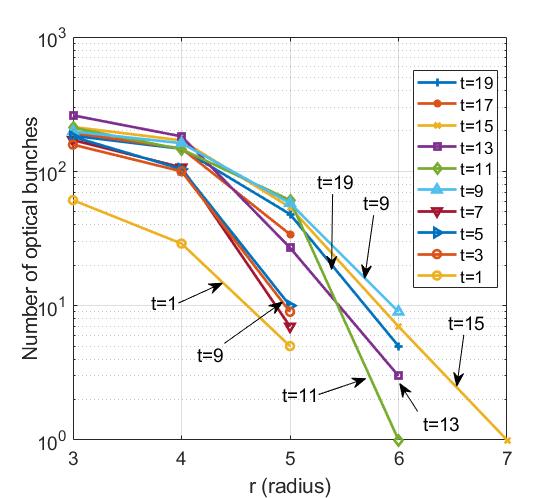
Figure 8: (Color on line) The number of the optical bunches vs. their width (radius $r$) at different times $t$, for the percolation probability $p=0.3$. It is seen that an increasing number of states with larger $r$ are created in the system in the course of the evolution.

While Fig. 8 displays typical dependences of the number of localized optical bunches, at different times, on the bunch’s width (radius) for the fixed percolation probability, $p=0.3$. Due to the statistical nature of the field localization, it is also relevant to calculate the time average of the dependencies shown in Fig. 8. These numerical results allows fitting to an analytical approximation with physically meaningful parameters. Accordingly, Fig. 9 shows a typical dependence the number of localized optical bunches averaged over the simulation time $t=20$ (blue asterisks) as a function of the bunch’s width (radius $r$) at fixed $p=0.30$.

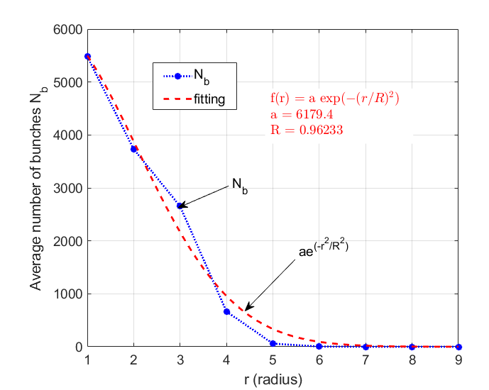
Figure 9: (Color on line) Blue asterisks: the number $N_{b}$ of localized optical bunches, averaged over $100$ different realizatins of the random system with $p=0.3$, for simulation time $t=20$, vs. the bunch’s radius $r$. The red dashed line shows the fitting function defined as per Eq. (9), with the fitting parameter $R$ representing the average width of the bunches. The error of the fitting is less than a few percents.

The red dashed line in Fig. 9 shows the fitting function,

$$f(r)=a\exp(-r^{2}/R^{2}),$$ (9)

with fitting parameters $a(p)$ and $R(p)$, where $R(p)$ is the average radius of the localized bunches at a fixed value of the percolation probability $p$. Additional computations demonstrates that the same fitting, with smooth functions $a(p)$ and $R(p)$, is equally accurate for other relevant values of the percolation probability $p$. The respective dependences $a(p)$ and $R(p)$ are plotted in Fig. 10. One observes in the figure that, close to $p=p_{\mathrm{cr}}\simeq 0.318$, there occurs a well-defined transition from the average bunch’s width $R=3$ to $R=1$. Recall that a narrow field structure with size $r=1$ corresponds to the point-like static field pinned to the emitter position. Thus, these results confirm the above conclusion that $p=p_{\mathrm{cr}}$ is the transition point (the mobility edge) which separates two different areas: at $p>p_{\mathrm{cr}}$ there exist only static fields pinned to the radiating nanoemitters, while at $\ p<p_{\mathrm{cr}}$ the dynamical localized field bunches emerge, which then migrate to the area free of emitters. The existence of a similar transition point was deduced in Ref. Burlak:2017 from different considerations, making use of the above-mentioned Ioffe-Regel criterion, $g=1$ [see Eq. (8)] for the 3D field localization. It is worthy to mention that probability $p\simeq 0.31$ is close to the percolation-transition point $p_{\mathrm{cr}}$ in the cubic 3D lattice Burlak:2017 , cf. Fig. 4.

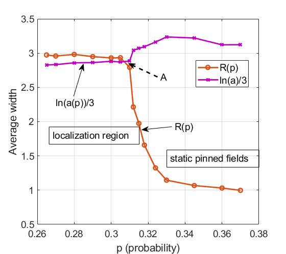
Figure 10: (Color online) The fitting parameters in Eq. (9) vs. the percolation probability $p$. Arrow A indicates the localization transition that matches to the critical point shown by arrow (A) in Fig. 4 and the percolating threshold $p_{c}$.

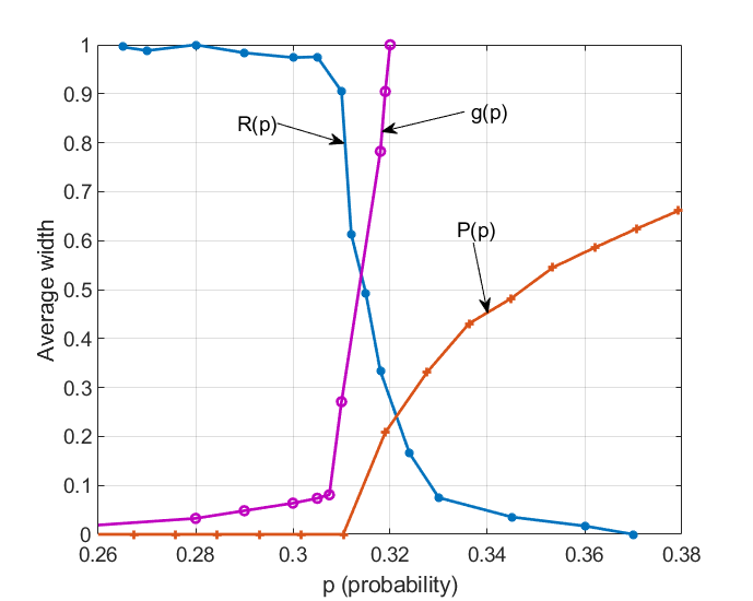
Figure 11: (Color online.) The comparison of the optical localization characteristics close to the percolation threshold $p_{c}=0.318$: the normalized average radius of the localized optical bunches, $R(p)$, the generalized conductivity, $g(p)$ [defined as per Eq. (8)], and the percolation order parameter Percolation , $P=P(p)$, vs. the percolation probability, $p$. The transition points produced by all these dependencies are quite close.

Different approaches are used above to identify the transition for the optical field in the percolating materials. It is instructive to compare the results produced by those approaches near the percolating threshold, $p_{\mathrm{cr}}=0.318$, for normalized average radius of the localized optical bunches, $R(p)$, generalized conductivity $g(p)$ [see Eq. (8)], and the percolation order parameter, $P(p)$, as functions of the percolation probability $p$ [the order parameter is defined as a probability that a particular site of the grid approximating the medium belongs to a percolation cluster piercing the entire sample Percolation . The comparison is produced in Fig. 10, which shows that the points of the localization transition, predicted by these different characteristics, are close to being identical.

VI Experimental studies of the emission spectra

In this Section we present experimental findings concerning optical radiation from nanoemitters incorporated in a porous ceramic matrix, which offers a realization of the setting considered above in the theoretical form.Our experimental study is based on the observation that an important mechanism for the generation of visible light is the up-conversion (UC) process by which at least two low-energy excitation photons, typically in the near infrared, are converted into one visible emission photon of higher energy, see Solis:2010a . In this case the strong green and red visible emissions can be obtained from ZrO${}_{2}:$ Yb⁺³ nanocrystals. The latter nanocrystals with different concentrations were incorporated into porous ceramics (approximately $1~{}$mm size) and then deposited on the inner surface of empty pores. The nanocrystals were prepared in three different configurations, (i) pure (undoped) ZnO2, (ii) ZnO2 dopped by Yb with $1.23\%$ concentration (hereafter referred to as sample E4), and (iii) ZnO₂ doped Yb at $2.36\%$ concentration (referred to as sample E5). For optical measurements, slices with size about $1~{}\mathrm{\mu}$m are cut from the bulk material. The optical measurements of absorption and emission spectra were performed for every sample.

Since the UC emission is strongly influenced by the content of Yb⁺³ ions, the embedded nanoemitters generate random emission, being excited by an external laser. The experimental setup is outlined in Fig. 12 (details of the technology used for synthesizing the nanoemitters are presented in Appendix).

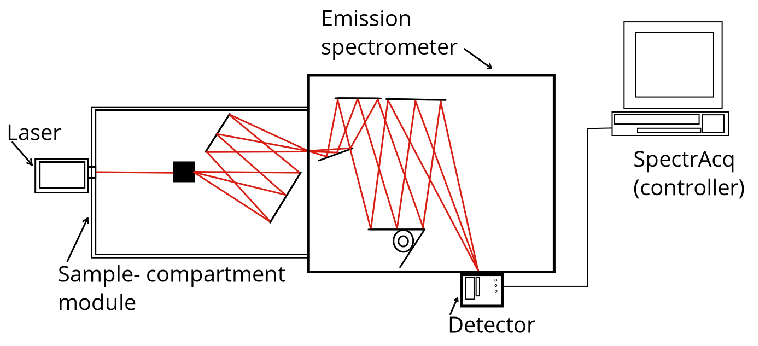
Figure 12: The scheme of the experimental setup built for measuring the emission spectrum. The small black square designates the sample.

We measured the emission spectra of the ceramic samples carrying the embedded undoped and Yb-doped nanocrystals, with the above-mentioned values of the dopant concentration, $1.23\%$ and $2.36\%$, respectively, using a Horiba Jobinyvon NanoLog FR3 spectrofluorometer Horiba . The samples were excited by an external $970$ nm pump. The beam emerging from the sample was coupled into the emission spectrometer module and finally passed to the detector. The signal from the detector was sent to the SpectrAcq controller for data processing.

It is seen that the emission bands for both samples with either value of the concentration are approximately located between $470$ and $570$ nm. It is observed too that the emission from the sample with the $2.36\%$ Yb concentration is $\approx 3$ times more intense than from the one with the $1.23\%$ concentration. Thus, it is demonstrated experimentally that the Yb-based nanocrystals incorporated in the porous ceramics emit in the green-wavelength range when the ceramic sample is excited by the external laser with the central wavelength of $970$ nm (see the inset in Fig. 13). Naturally, the radiation intensity increases with the growth of the concentration of nanocrystals in the ceramic host material.

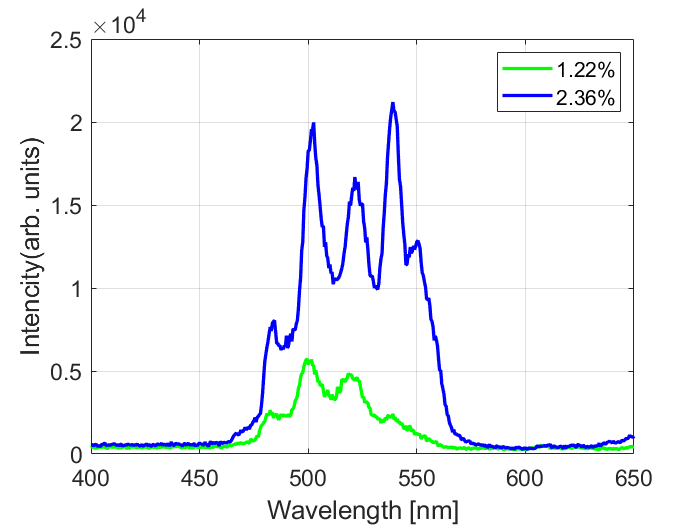
Figure 13: Emission spectra (in arbitrary units) of the Yb-doped ceramics with different Yb concentrations, viz., $1.23\%$ (see details in the text).

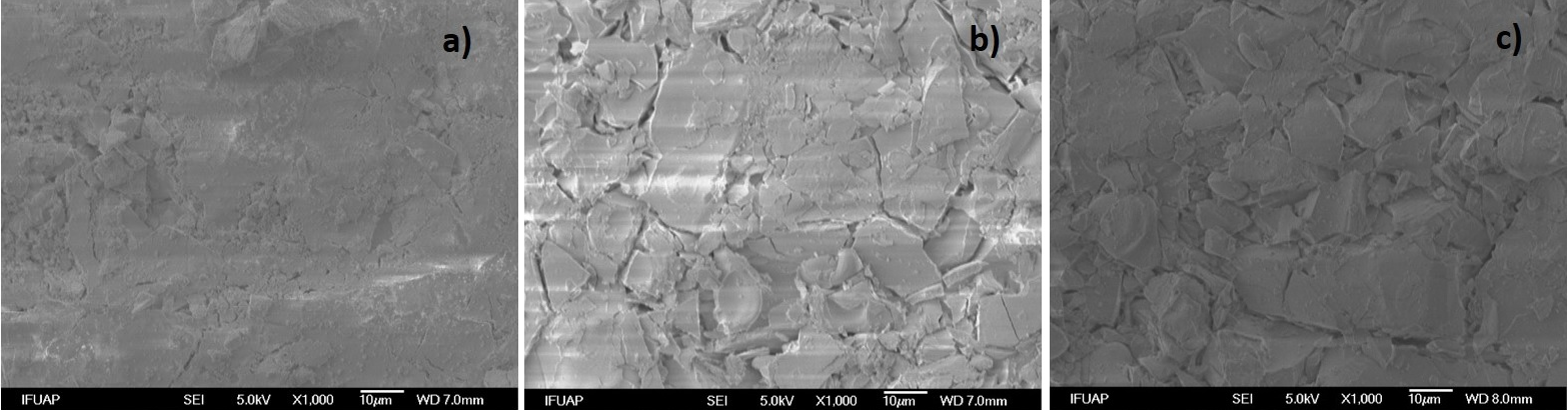
Figure 14: SEM images of a) the undoped ZrO₂ sample, and doped ones, E4 and E5, with the Yb concentration $1.23$% [panel b)], and $2.36$% [panel c)], respectively.

Figure 14 shows the SEM (scanning-electron-microscope) image of the surface morphology of the undoped ZrO₂ sample and Yb-doped ones (E4 and E5 correspond to the $1.23$% and $2.33$% dopant concentrations, respectively). Figure 14 demonstrates that the porosity of the samples increases with the increase of the Yb concentration, in comparison with the undoped sample, which is displayed in Fig. 14a). The aggregate sizes of samples E4 and E5, composed of small crystals, are similar, taking values between $10$ and $30$ $\mathrm{\mu}$m, while more grain boundaries are observed in E5, see Fig. 14c), hence the latter one has a higher level of porosity. The average pore sizes for the samples are $1$ $\mathrm{\mu}$m, $0.5$ $\mathrm{\mu}$m, and $2~{}\mathrm{\mu}$m for a) undoped ZrO₂, and doped samples, viz., E4 in b) and E5 in c), respectively. From the X-ray diffractograms (XRD) and the Debye-Scherrer equation Ingham:2015a , the crystalline sizes extracted from Fig. 14 can be evaluated as $69.8~{}$nm in a), $72.6~{}$nm in b), and $65.9~{}$nm in c). 

VII Conclusion

We have predicted theoretically and confirmed experimentally that the localization of the optical field in the active three-dimensional disordered percolating system has a nontrivial structure, allowing the generation and propagation of localized field bunches. The system includes randomly distributed nanoemitters, which, in general, corresponds to a spatially averaged percolation environment. The localization strength and average width of the corresponding structures have been analyzed, and that the transition between the propagating bunches and point-like fields pinned to the radiating emitters has been identified. The optical emission spectrum from nanoemitters incorporated in the porous ceramic medium, measured in our experiment, is in reasonable agreement with the prediction of the theory.

The analysis in this work is mainly concentrated on the emission pattern in the frequency domain. As an extension of the work, we will study its counterpart in the time domain, which requires the use of a more advanced experimental technique.

Disclosures

The authors declare no conflicts of interest.

Data Availability Statement

Data that support the theoretical and experimental findings of this study are available from the corresponding author upon a reasonable request.

Appendix: The synthesis of sol-gel nanocrystals at room temperatures

Ytterbium-doped zirconium nanocrystals were fabricated using the sol-gel method. The produced nanocrystals feature different Yb percentages and were characterized by EDS (energy dispersive spectrometry), XRD (X-ray diffraction), and UV-Vis NIR (ultraviolet-visible near infrared) spectroscopy. Note that in the theoretical part it was proposed to use pores in the host ceramic medium to create a hybrid solid system with integrated nanoemitters. However, in the experiment such a method is quite time-consuming. It can be replaced by the following simple direct technique. To create a hybrid mixture with incorporated nanoemitters, we apply the well-known Sol-Gel technique sol-gel , which makes it possible to make hybrid medium directly by mixing the zirconium and the dopant. [I have inserted here an obviously missing reference to the sol-gel technique.] For this purpose, a mixture of $1.0$ equivalent of zirconium n-propoxide ($70\%$) in absolute ethanol ($20$ equivalents) was stirred (“agitated”) for two minutes, and then $0.1$ equivalents of HNO₃ ($67\%$) were drop-wise added under intensive agitation. After that, $0.3$ equivalent of HCl ($37\%$) was added under agitation too. A solution of $0.043$ equivalent of ytterbium chloride-YbCl₃6H₂O ($99.99\%$) in $2$ mL of ethanol was added to the mixture, agitated during $60$ min to produce the gel phase, and dried at $100^{\mathrm{o}}$ C for 24 hours. The sample was annealed at $1000^{o}$ C for 10 hours. The solid product was obtained in the form of fine white particles with $1.23\%$ of ytterbium determined by EDS. When $0.087$ equivalents of YbCl₃6H₂O were added, the obtained product featured $2.36\%$ of ytterbium. A hydropneumatic press was used to obtain the product in the form of thin ceramic pellets, which were used for the absorption characterization.

References

- [1] Francesco Riboli, Niccolò Caselli, Silvia Vignolini, Francesca Intonti, Kevin Vynck, Pierre Barthelemy, Annamaria Gerardino, Laurent Balet, Lianhe H. Li, Andrea Fiore, Massimo Gurioli, and Diederik S. Wiersma. Engineering of light confinement in strongly scattering disordered media. Nat. Mater., 13(7):720–725, Jul 2014.
- [2] Kevin Vynck, Matteo Burresi, Francesco Riboli, and Diederik S. Wiersma. Photon management in two-dimensional disordered media. Nat. Mater., 11(12):1017–1022, Dec 2012.
- [3] S. Flach, D. O. Krimer, and Ch. Skokos. Universal spreading of wave packets in disordered nonlinear systems. Phys. Rev. Lett., 102:024101, Jan 2009.
- [4] Ping Sheng. Introduction to Wave Scattering, Localization and Mesoscopic Phenomena, volume 88 of Springer Series in Materials Science. Springer, Berlin, 2006.
- [5] Jing Wang and Azriel Z. Genack. Transport through modes in random media. Nature (London), 471(7338):345–348, Mar 2011.
- [6] F. Jendrzejewski, A. Bernard, K. Muller, P. Cheinet, V. Josse, M. Piraud, L. Pezze, L. Sanchez-Palencia, A. Aspect, and P. Bouyer. Three-dimensional localization of ultracold atoms in an optical disordered potential. Nat. Phys., 8(5):398–403, May 2012.
- [7] Mordechai Segev, Yaron Silberberg, and Demetrios N. Christodoulides. Anderson localization of light. Nat. Photon., 7(3):197–204, Mar 2013.
- [8] Diederik S. Wiersma. Disordered photonics. Nat. Photon., 7(3):188–196, Mar 2013.
- [9] Bernard R. Matis, Steven W. Liskey, Nicholas T. Gangemi, Aaron D. Edmunds, William B. Wilson, Virginia D. Wheeler, Brian H. Houston, Jeffrey W. Baldwin, and Douglas M. Photiadis. Observation of a transition to a localized ultrasonic phase in soft matter. Communications Physics, 5:21, 2022.
- [10] S. E. Skipetrov and I. M. Sokolov. Ioffe-regel criterion for anderson localization in the model of resonant point scatterers. Phys. Rev. B, 98:064207, Aug 2018.
- [11] L. A. Cobus, W. K. Hildebrand, S. E. Skipetrov, B. A. van Tiggelen, and J. H. Page. Transverse confinement of ultrasound through the anderson transition in three-dimensional mesoglasses. Phys. Rev. B, 98:214201, Dec 2018.
- [12] P. W. Anderson. Absence of diffusion in certain random lattices. Phys. Rev., 109:1492–1505, Mar 1958.
- [13] S. E. Skipetrov. Finite-size scaling analysis of localization transition for scalar waves in a three-dimensional ensemble of resonant point scatterers. Phys. Rev. B, 94:064202, Aug 2016.
- [14] Sanli Faez, Anatoliy Strybulevych, John H. Page, Ad Lagendijk, and Bart A. van Tiggelen. Observation of multifractality in anderson localization of ultrasound. Phys. Rev. Lett., 103:155703, Oct 2009.
- [15] Salman Karbasi, Craig R. Mirr, Parisa Gandomkar Yarandi, Ryan J. Frazier, Karl W. Koch, and Arash Mafi. Observation of transverse anderson localization in an optical fiber. Opt. Lett., 37(12):2304–2306, Jun 2012.
- [16] Dietrich Stauffer and Ammon Aharony. Introduction to percolation theory. Taylor & Francis, London, 2003.
- [17] Juliette Billy, Vincent Josse, Zhanchun Zuo, Alain Bernard, Ben Hambrecht, Pierre Lugan, David Clement, Laurent Sanchez-Palencia, Philippe Bouyer, and Alain Aspect. Direct observation of Anderson localization of matter waves in a controlled disorder. Nature (London), 453(7197):891–894, Jun 2008.
- [18] G. Burlak, M. Vlasova, P.A. Márquez Aguilar, M. Kakazey, and L. Xixitla-Cheron. Optical percolation in ceramics assisted by porous clusters. Opt. Commun., 282(14):2850 – 2856, 2009.
- [19] Gennadiy Burlak and Y. G. Rubo. Mirrorless lasing from light emitters in percolating clusters. Phys. Rev. A, 92:013812, Jul 2015.
- [20] G. Burlak and E. Martinez-Sánchez. The optical Anderson localization in three-dimensional percolation system. Opt. Commun., 387:426 – 431, 2017.
- [21] A. E. Siegman. Lasers. University Science Books, Sausalito, 1986.
- [22] Xunya Jiang and C. M. Soukoulis. Time dependent theory for random lasers. Phys. Rev. Lett., 85:70–73, Jul 2000.
- [23] Yang Hao and Raj Mittra. FDTD Modeling of Metamaterials Theory and Application. Artech House, Norwood MA, 2009.
- [24] Azriel Z. Genack and Jing Wang. Speckle statistics in the photon localization transition. In Elihu Abrahams, editor, 50 years of Anderson localization, chapter 22, pages 559–597. World Scientific Publishing, Singapore, 2010.
- [25] William H Press, Saul A Teukolsky, William T Vettering, and Brian P Flannery. Numerical recipes example book (c++): The art of scientific computing. Cambridge University Press, Cambridge, 2002.
- [26] AF Ioffe and AR Regel. Non-crystalline, amorphous, and liquid electronic semiconductors. In Progress in semiconductors, pages 237–291. Wiley, New York, 1960.
- [27] Junfeng Wang, Zongzheng Zhou, Wei Zhang, Timothy M. Garoni, and Youjin Deng. Bond and site percolation in three dimensions. Phys. Rev. E, 87:052107, May 2013.
- [28] Allen Hunt, Robert Ewing, and Behzad Ghanbarian. Percolation theory for flow in porous media, volume 880. Springer, 2014.
- [29] D. Solis, E. De la Rosa, O. Meza, L. A. Diaz-Torres, P. Salas, and C. Angeles-Chavez. Role of Yb3+ and Er3+ concentration on the tunability of green-yellow-red upconversion emission of codoped ZrO2:Yb3+–Er3+ nanocrystals. Journal of Applied Physics, 108(2), 07 2010. 023103.
- [30] Horiba Scientific. Steady state and lifetime nanotechnology eem spectrofluorometer. In Modular Nanolog Spectrofluorometer is specifically designed for research in nanotechnology and nanomaterials. Horiba, 2021.
- [31] Bridget Ingham. X-ray scattering characterisation of nanoparticles. Crystallography Reviews, 21(4):229–303, 2015.
- [32] H Schmidt and Lisa C Klein. Sol-gel optics. processing and applications, 1994.