Quantum Parallelized Variational Quantum Eigensolvers for Excited States

Abstract

Calculating excited-state properties of molecules and solids is one of the main computational challenges of modern electronic structure theory. By combining and advancing recent ideas from the field of quantum computing we propose a more effective variational quantum eigensolver based on quantum parallelism: Initial ansätze for various excited states are prepared into a single pure state through a minimal number of ancilla qubits. Then a global rotation in the targeted subspace is optimized. Our approach thus avoids the progressive accumulation of errors prone to schemes that calculate excited states successively. Energy gaps and transition amplitudes between eigenstates can immediately be extracted. Moreover, the use of variable auxiliary weights makes the algorithm more resilient to noise and greatly simplifies the optimization procedure. We showcase our algorithm and illustrate its effectiveness for different molecular systems. The interaction effects are treated through generalized unitary coupled cluster ansätze and, accordingly, the common unfavorable and artificial extension to the entire Fock space is circumvented.

I Introduction

Describing and understanding excited-state properties of atoms, molecules, and solids, is one of the most important challenges of modern electronic structure theory. While state-of-the-art methodologies can reach a great degree of accuracy for molecular ground states at equilibrium, excited states present themselves as a major computational bottleneck for at least two reasons: the many types of qualitatively different electronic excitations present in chemical processes (valence, Rydberg, or vertical, to list a few) and their inherent stronger multi-configurational character, expanding thus into quite large parts of the Hilbert space González et al. (2012); Onida et al. (2002); Serrano-Andrés and Merchán (2005); Westermayr and Marquetand (2021); Loos et al. (2018); Ghosh et al. (2018). This also makes their manipulation and storage very inefficient on classical computers González and Lindh (2020). A promising strategy to overcome some of these problems is to use quantum devices, whose disruptive potential lies precisely in their capability of representing and manipulating quantum states in such challenging physical setups Cirac and Zoller (2012); Preskill (2018). The possibility of controlling highly multiconfigurational wave functions in near-term quantum technologies has recently made the development of hybrid quantum-classical algorithms for excited states an active field of research Xie et al. (2022); Parrish et al. (2019); Ollitrault et al. (2020); Lyu et al. (2023); Colless et al. (2018); Gocho et al. (2023); Tazi and Thom (2023); Head-Marsden et al. (2021).

Hybrid quantum-classical algorithms were first developed for chemical ground states. Chief among them is the variational quantum eigensolver (VQE) Peruzzo et al. (2014). It prepares trial wave functions on a quantum circuit and optimizes their parameters self-consistently using classical devices, requiring short coherence times in the execution of the circuit McClean et al. (2016a); Fedorov et al. (2022). In virtue of generalized variational principles, several approaches were proposed for calculating excited states in the realm of VQE Cao et al. (2019); Santagati et al. (2018); McArdle et al. (2020); McClean et al. (2017a); Zhang et al. (2022); Wang and Mazziotti (2023). Two of the most prominent, yet conceptually different ones, are the variational quantum deflation (VQD) algorithm and the subspace-search VQE (SSVQE). VQD targets excited states successively: the $K$-th excited state is calculated variationally from the original Hamiltonian modified by suitable energy penalties for the first $K$ eigenstates $\mbox{$|0\rangle$},\ldots,\mbox{$|K-1\rangle$}$, determined beforehand Higgott et al. (2019); Jones et al. (2019); Ibe et al. (2022); Wen et al. (2021); Shirai et al. (2022). In contrast, SSVQE identifies in the first place just the subspace spanned by the $K$ lowest-lying eigenstates. For this, a unitary is sought which rotates $K$ orthogonal initial states in such a way that the average energy of the resulting states is minimized Nakanishi et al. (2019); Yalouz et al. (2021).

While the significance of VQD and SSVQE in the context of quantum computing can hardly be overestimated, they are both plagued by a number of unpleasant limitations and shortcomings. For instance, to determine the $K$-th eigenstate, VQD needs to calculate each of the first $K-1$ eigenstates in separate, preceding calculations. Even worse, as $K$ increases its numerical predictability deteriorates due to an intrinsic accumulation of errors Kuroiwa and Nakagawa (2021). Those deficiencies are overcome by SSVQE in the sense that the orthogonality is fulfilled automatically. The resulting individual eigenstates, however, are optimal only on average, without control over the errors, and their calculation in the first place required additional classical or quantum resources. It will be the ultimate accomplishment of our work to propose a quantum eigensolver for computing excited states which overcomes these and related shortcomings and limitations. In order to achieve this, we exploit the effect of quantum parallelism to variationally determine various excited states simultaneously, rather than individually in separate calculations. At the same time, flexible auxiliary weights still provide full access to various individual states. Due to this and the distinctive nature of our VQE — the simultaneous preparation of various excited states — crucial physical quantities such as energy gaps and transition amplitudes between eigenstates can subsequently be extracted in a straightforward manner.

The structure of the paper is as follows. In Sec. II, we recap in more detail the VQD and SSVQE and their shortcomings. The latter motivates our approach which we then present on a conceptual level in Sec. III. In Sec. IV, we discuss practical aspects, in particular, the implementation of our algorithm and compare its computational cost to those of other known algorithms. Numerical experiments are presented in Sec. V together with an analysis of the effect of noisy gates on our results. Additional technical details are presented in three Appendices.

II Hybrid quantum-classical methods for excited states

In this section, we recall in more detail the most prominent VQEs established in recent years for computing excited states. A particular emphasis lies on their strengths and weaknesses which in turn motivate our more effective VQE to be proposed in the subsequent sections.

In the original VQE algorithm, a set of variational parameters $\bm{\theta}$ is optimized on a classical device. These parameters are used to parameterize a quantum circuit and a respective unitary $U(\bm{\theta})$ that transforms an initial reference state $|\phi\rangle$ to a quantum state $\mbox{$|\psi(\bm{\theta})\rangle$}=U(\bm{\theta})\mbox{$|\phi\rangle$}$. To calculate the ground state $|\psi(\bm{\theta}^{\ast})\rangle$ of a given Hamiltonian $\hat{H}$, the optimal parameters $\bm{\theta}^{*}$ are thus found by minimizing the corresponding energy expectation value

$$E(\bm{\theta})=\mbox{$\langle\psi(\bm{\theta})|$}\hat{H}\mbox{$|\psi(\bm{\theta})\rangle$}\,.$$ (1)

By exploiting the orthogonality of the eigenstates of $\hat{H}$, VQD adds a sequence of penalty terms to the VQE cost function $E(\bm{\theta})$ to estimate excited states Higgott et al. (2019). The effective Hamiltonian for such an optimization of the $K$-th excited state is given by

$$\hat{H}_{K}(\bm{\theta}_{0},\ldots,\bm{\theta}_{K-1})=\hat{H}+\sum^{K-1}_{j=0}\beta_{j}\mbox{$|\psi_{j}(\bm{\theta}_{j})\rangle$}\mbox{$\langle\psi_{j}(\bm{\theta}_{j})|$}\,.$$ (2)

For sufficiently large positive values $\beta_{j}$, this is equivalent to minimizing the energy of the $K$-th excited state $E_{K}(\bm{\theta}_{K})=\mbox{$\langle\psi_{K}(\bm{\theta}_{K})|$}\hat{H}\mbox{$|\psi_{K}(\bm{\theta}_{K})\rangle$}$ subject to the constraint that the minimizer is orthogonal to the states $|\psi_{0}(\bm{\theta}_{0})\rangle$,…, $|\psi_{K-1}(\bm{\theta}_{K-1})\rangle$. The $K$-th eigenstate becomes the ground state of the respective effective Hamiltonian (2). While there are ways to determine the magnitude of the penalty terms $\beta_{0},\ldots,\beta_{K-1}$, leading to faster convergence in the optimization of $\bm{\theta}$ Kuroiwa and Nakagawa (2021), VQD requires in addition all ansätze $|\psi_{j}(\bm{\theta}_{j})\rangle$ to be sufficiently expressive. As a result, a progressive accumulation of errors seems to be unavoidable, especially for the calculation of highly excited states. In a rather similar fashion, the orthogonal state reduction VQE (OSRVE) computes the $K$-th state by eliminating contributions of the lower eigenstates Xie et al. (2022). Instead of requiring penalty terms, OSRVE enforces orthogonality through auxiliary qubits that are added to the circuit. Yet, in complete analogy to VQD, OSRVE requires $K$ rounds of optimization to compute the $K$ energetically lowest eigenenergies and the numerical predictability deteriorates as $K$ increases.

In contrast to VQD and OSRVE, SSVQE in its original form seeks in a first step just the subspace spanned by the first $K$ eigenstates. This is realized in practice through the following state-average calculation. One chooses $K$ initial orthogonal states $\mbox{$|\phi_{0}\rangle$},\ldots,\mbox{$|\phi_{K-1}\rangle$}$, which are then rotated through a unitary $U(\bm{\theta})$ in order to minimize their energy average. This “democratic” distribution of those states results in the corresponding cost function Nakanishi et al. (2019); Yalouz et al. (2021); Xu et al. (2023):

$$\mathcal{L}(\bm{\theta})=\sum^{K-1}_{j=0}\mbox{$\langle\phi_{j}|$}U^{\dagger}(\bm{\theta})\hat{H}U(\bm{\theta})\mbox{$|\phi_{j}\rangle$}\,.$$ (3)

While the orthogonality of various optimized $U(\bm{\theta}^{\ast})\mbox{$|\phi_{j}\rangle$}$ is guaranteed, these individual states are optimal only on average. Indeed, since all states possess equal weight, the cost function (3) is invariant under unitary rotations among them. Hence, an additional optimization scheme within this subspace is necessary to extract the individual eigenstates. An advanced variant of SSVQE assigns distinct weights $w_{j}$ to the subspace states in order to make these supplementary optimization stages obsolete. Then, the generalization of the Rayleigh-Ritz variational principle to ensemble states with spectrum $\bm{w}=(w_{0},\ldots,w_{K-1})$, where $w_{j}>w_{j+1}$ Gross et al. (1988a), guarantees that the energy expectation of the energies is bounded from below by the weighted sum of the eigenenergies,

$$\sum^{K-1}_{j=0}w_{j}\mbox{$\langle\phi_{j}|$}U^{\dagger}(\bm{\theta})\hat{H}U(\bm{\theta})\mbox{$|\phi_{j}\rangle$}\geq\sum^{K-1}_{j=0}w_{j}E_{j}\,,$$ (4)

with $E_{j}\leq E_{j+1}$ being the exact eigenenergies of the system. This ensemble variational principle, which provides the theoretical foundation of weighted SSVQE, offers a unified variational approach to quantum mechanics. The variational principle for ground states is, in fact, just a particular case, corresponding to $\bm{w}=(1,0,0,\ldots)$. The significance of this variational approach has also been recognized in the context of functional theories, where it is being intensively employed (see, e.g., Fromager (2020); Schilling and Pittalis (2021); Liebert et al. (2022); Gould et al. (2023); Liebert and Schilling (2023); Cernatic et al. (2021) and references therein).

The advantages of the weighted SSVQE are rather obvious. Relative to VQD and OSRVE, there is no need anymore to enforce the orthogonality constraint of the states through penalty terms which in turn simplifies the underlying cost function. The optimization of the quantum circuit runs only once, again in stark contrast to VQD and OSRVE which both require $K$ subsequent optimizations. Finally, the spectrum can be exactly reached as long as the quantum circuit has the sufficient expressive power to represent the unitary which maps the input states $|\phi_{j}\rangle$ to the sought-after eigenstates $\mbox{$|\psi_{j}(\bm{\theta}^{*})\rangle$}=U(\bm{\theta}^{*})\mbox{$|\phi_{j}\rangle$}$ of $\hat{H}$ Ding et al. (2023). However, to compute the SSVQE cost function, $K$ different expectation values are needed in each step (namely, $E_{j}(\bm{\theta})=\mbox{$\langle\psi_{j}(\bm{\theta})|$}\hat{H}\mbox{$|\psi_{j}(\bm{\theta})\rangle$}$), resulting in run-time overhead.

From a more general conceptual perspective, neither weighted SSVQE nor any of the other discussed VQEs prepare a quantum state which contains the information about various excited states simultaneously. This would be necessary, however, to determine in a straightforward manner physically relevant quantities such as energy gaps and transition amplitudes between various eigenstates. Moreover, as far as the performance of all these algorithms is concerned, the problem of violating symmetries is even more crucial for excited states than for ground states Seki et al. (2020); Lyu et al. (2023). Symmetries in VQE-based algorithms are usually enforced so far either through circuits that respect these symmetries or by adding extra penalty terms to the cost function. While the former strategy could be rather unpractical Lyu et al. (2020), the latter requires prior knowledge of various symmetries Ryabinkin et al. (2019); Kuroiwa and Nakagawa (2021).

In summary, while all these algorithms represent a landmark in the development of quantum computation for excited states, they leave a lot of room for improvement. We summarize their main shortcomings:

• numerical errors are progressively accumulated as a result of the subsequent computations of various eigenstates,

• determining various eigenstates from a preceding calculation of their spanned subspace requires additional rounds of quantum or classical optimization,

• energy expectation values of individual states need to be summed up in the cost functions which results in run-time overhead at the level of circuit executions, and

• the information about various excited states is never simultaneously present in the circuit and thus energy gaps and transition amplitudes between eigenstates cannot be extracted immediately in a straightforward manner.

Although some algorithms overcome some of these issues, they altogether hamper the development of a unified efficient strategy to compute excited-state properties of many-body systems on near-term quantum devices. As we will discuss in the next section, our proposed quantum-parallelization of VQEs offers a comprehensive solution to the above problems.

III Quantum parallelism and variational computation of excited states

In this section, we introduce our novel VQE for excited states on a conceptual level, while its implementation and technical features are discussed in Section IV.

Our algorithm is designed in such a way that it calculates the weighted cost function

$$\mathcal{L}_{\bm{w}}(\bm{\theta})\equiv\sum_{j}w_{j}E_{j}(\bm{\theta}) = \sum^{K-1}_{j=0}w_{j}\mbox{$\langle\phi_{j}|$}U^{\dagger}(\bm{\theta})\hat{H}U(\bm{\theta})\mbox{$|\phi_{j}\rangle$}$$ (5)

$$= \mbox{Tr}[\hat{H}U(\bm{\theta})\rho(\bm{w})U^{\dagger}(\bm{\theta})]$$

in a direct manner through the mixed quantum state

$$\rho(\bm{w})=\sum_{j=0}^{K-1}w_{j}\mbox{$|\phi_{j}\rangle$}\mbox{$\langle\phi_{j}|$}\,,$$ (6)

with the normalization condition $\sum_{j}w_{j}=1$. In order to achieve this on a unitary quantum circuit, the underlying key idea is to map this state into a single quantum state

$$\rho(\bm{w})\xrightarrow{\mathrm{purification}}\mbox{$|\Phi(\bm{w})\rangle$}=\sum_{j}\sqrt{w_{j}}\,\mbox{$|\phi_{j}\rangle$}\otimes\mbox{$|a_{j}\rangle$}\,.$$ (7)

The auxiliary states $|a_{j}\rangle$ are added to execute the parallelization of the eigenstates. The only formal requirement on $|a_{i}\rangle$ is the orthonormality condition $\langle{a_{i}}\mbox{$|a_{j}\rangle$}=\delta_{ij}$. As a consequence, $\langle\Phi(\bm{w})\mbox{$|\Phi(\bm{w})\rangle$}=1$, and more generally one finds that for any observable $\hat{A}$

$$\mbox{$\langle\Phi(\bm{w})|$}\hat{A}\otimes\openone\mbox{$|\Phi(\bm{w})\rangle$} =\sum_{ij}\sqrt{w_{i}w_{j}}\mbox{$\langle\phi_{i}|$}\hat{A}\mbox{$|\phi_{j}\rangle$}\langle a_{i}\mbox{$|a_{j}\rangle$}$$

$$=\sum_{i}w_{i}\mbox{$\langle\phi_{i}|$}\hat{A}\mbox{$|\phi_{i}\rangle$}$$

$$=\mbox{Tr}[\hat{A}\rho(\bm{w})]\,.$$ (8)

Then, $|\Phi(\bm{w})\rangle$ can be used to recover the cost function (5) which in turn can be rewritten as

$$\mathcal{L}_{\bm{w}}(\bm{\theta})=\mbox{$\langle\Phi(\bm{w})|$}[U^{\dagger}(\bm{\theta})\hat{H}U(\bm{\theta})]\otimes\openone\mbox{$|\Phi(\bm{w})\rangle$}\,.$$ (9)

We believe this way of thinking about quantum spectra — which is possible because of the linearity of quantum mechanics — is not only conceptually more appealing but also computationally more efficient. To be more specific, using the state (7) as the starting point for the variational calculation of the parameters through the cost function $\mathcal{L}_{\bm{w}}(\bm{\theta})$ has the following advantages. First, since optimizing the cost function involves the simultaneous rotation of various eigenstates it can be calculated in one shot, in contrast to, e.g., weighted SSVQE which sums up energies $E_{j}(\bm{\theta})$ obtained in $K$ separate shots. Second, the set $\bm{w}$ of flexible auxiliary weights allows one to control the error ranges of various energy levels systematically and provides direct access to various individual eigenstates. Third, since various eigenstates are prepared simultaneously on a quantum device our scheme facilitates the direct calculation of energy gaps and transition amplitudes between eigenstates. Because of these promising features and due to the key role of quantum parallelism therein we refer to our proposed approach in the following as Quantum Parallelized Variational Quantum Eigensolver (QP-VQE). In particular, we feel that the emphasis on quantum parallelism and the simultaneous preparation of various excited states could stimulate computational advances in terms of both extended scope and improved numerical efficiency.

Another important feature of QP-VQE is a remarkable degree of flexibility offered by the initial quantum state (7). For instance, if each state $|a_{j}\rangle$ is chosen as an exact replica of $|\phi_{j}\rangle$ the new Hilbert space is a twin version of the original one Israel (1976); Takahashi and Umezawa (1996); Borrelli and Gelin (2021); Benavides-Riveros et al. (2022). If, in addition, the initial states are Slater determinants (e.g., the Hartree-Fock solutions), the pure state $|\Phi(\bm{w})\rangle$ can be represented as the well-known Bardeen-Cooper-Schrieffer (BCS) state of conventional superconductivity Benavides-Riveros et al. (2022): $\mbox{$|\Phi_{\rm BCS}(\bm{w})\rangle$}=\prod_{m}\left(\sqrt{1-w_{m}}+\sqrt{w_{m}}c^{\dagger}_{m}\tilde{c}^{\dagger}_{m}\right)\mbox{$|0\rangle$}$, where $c_{m}^{\dagger}$ and $\tilde{c}_{m}^{\dagger}$ are (real and fictitious) fermionic creation operators for mode $m$. Noteworthy, if the unitary ansatz $U(\bm{\theta})$ employed in Eq. (5) is sufficiently expressive, the process of optimizing the cost function $\mathcal{L}_{\bm{w}}(\bm{\theta})$ will always yield eigenstates with the correct physical symmetries. Furthermore, the squeezed representation of the BCS state $\mbox{$|\Phi_{\rm BCS}(\bm{w})\rangle$}=V(\bm{w})\mbox{$|0\rangle$}$, with the unitary $V(\bm{w})=\exp\big{[}\sum_{m}\vartheta_{m}(c^{\dagger}_{m}\tilde{c}^{\dagger}_{m}-\tilde{c}_{m}c_{m})\big{]}$ and $\sin(\vartheta_{m})=\sqrt{w_{m}}$, results in an efficient representation of the cost function $\mathcal{L}^{\rm BCS}_{\bm{w}}(\bm{\theta})=\mbox{$\langle 0|$}U_{\bm{w}}^{\dagger}(\bm{\theta})\hat{H}_{\bm{w}}U_{\bm{w}}(\bm{\theta})\mbox{$|0\rangle$}$, where $\hat{A}_{\bm{w}}=V(\bm{w})^{\dagger}\hat{A}V(\bm{w})$ is a Bogoliubov transformation of the operator $\hat{A}$ and $|0\rangle$ is the real vacuum of the double system (i.e., $c_{m}\mbox{$|0\rangle$}=\tilde{c}_{m}\mbox{$|0\rangle$}=0$). This representation resembles the much simpler cost function of the standard ground-state VQE. Yet, it is also worth noticing that this approach based on the BCS state involves an extension of the electron correlation problem at hand to the entire Fock space. While this is certainly reasonable in the context of macroscopic systems with indefinite particle numbers, it is rather artificial and disadvantageous for microscopic molecular systems as studied in quantum chemistry.

From a more general perspective, the states $|a_{j}\rangle$ can be associated with any kind of auxiliary Hilbert space, be it the Fock space of a single bosonic mode or a sequence of ancilla qubits. All these types of quantum parallelizations allow us to represent the eigenstates we are interested in as a single quantum state which can be implemented directly in a quantum circuit.

Finally, enforcing a given symmetry $\hat{s}$ in the cost function is also possible in our quantum parallelized one-shot scenario. Indeed, instead of computing a cost function for each individual state as it is usually done both in VQE and VQD (i.e., $\mathcal{L}_{j}(\bm{\theta})=\mbox{$\langle\psi_{j}(\bm{\theta})|$}(\hat{s}-\mbox{$\langle\psi_{j}(\bm{\theta})|$}\hat{s}\mbox{$|\psi_{j}(\bm{\theta})\rangle$})^{2}\mbox{$|\psi_{j}(\bm{\theta})\rangle$}$), we could utilize $\mbox{$\langle\Phi^{\prime}(\bm{w})|$}\mathcal{U}^{\dagger}(\bm{\theta})\hat{S}\,\mathcal{U}(\bm{\theta})\mbox{$|\Phi^{\prime}(\bm{w}\rangle$}$, where $\hat{S}=\hat{s}^{2}\otimes\openone\otimes\openone-\hat{s}\otimes\hat{s}\otimes\openone$, $\mathcal{U}(\bm{\theta})=U(\bm{\theta})\otimes U(\bm{\theta})\otimes\openone$, and $\mbox{$|\Phi^{\prime}(\bm{w})\rangle$}=\sum_{j}\sqrt{w_{j}}\,\mbox{$|\phi_{j}\rangle$}\otimes\mbox{$|\phi_{j}\rangle$}\otimes\mbox{$|a_{j}\rangle$}$ would be a generalization of the state (7). This way of computing fluctuation of observables, by doubling the Hilbert space, has already prominently been used in the context of tensor network ansätze for quantum spectra Pollmann et al. (2016). For quantum devices, the preparation of this kind of state has been discussed in Refs. Sagastizabal et al. (2021); Sager and Mazziotti (2022); Wu and Hsieh (2019).

IV Implementation and Features of QP-VQE

IV.1 Initial state preparation

As it was outlined in the previous section, the BCS quantum state $|\Phi_{\rm BCS}(\bm{w})\rangle$ could be useful for dealing with a significant part of the spectrum on the Fock space. This state, however, artificially breaks the particle-number symmetry. Although breaking symmetries enhances the variational flexibility which is known to be beneficial for the study of strong-correlation regimes, their restoration after the optimization is usually quite involved Khamoshi et al. (2022); Jiménez-Hoyos et al. (2012); Khamoshi et al. (2023). Moreover, we are often interested in the spectrum of a specific particle-number symmetry sector; and in practice, the unitary ansatz is never large and expressive enough to cover all transformations in the Fock space. Therefore, whenever the Hamiltonian in question exhibits symmetries it is always instructive to start from states with the desired symmetry and apply unitaries that respect it.

To describe the state preparation of the QP-VQE, we start with $M$ real value orthogonal spatial orbitals $|f_{p}\rangle$, with $p=0,\ldots,M-1$. Under the spin-restricted formalism, we define the corresponding $\alpha$ ($\beta$) spin-orbitals denoted as $|f_{p}\rangle$$|\alpha\rangle$ (and $|f_{p}\rangle$$|\beta\rangle$) for each spatial orbital, resulting in a total of $N=2M$ spin orbitals. In the Jordan-Wigner (JW) encoding Jordan and Wigner (1928), the occupation number of a spin-orbital is represented by the states $|0\rangle$ or $|1\rangle$ of a corresponding qubit state (unoccupied and occupied, respectively). An ‘interleaved’ ordering is utilized to assign numbers to the qubits such that $\mbox{$|f_{0\alpha}\rangle$},\mbox{$|f_{0\beta}\rangle$},\ldots,\mbox{$|f_{(M-1)\alpha}\rangle$},\mbox{$|f_{(M-1)\beta}\rangle$}$. The reference states $|\phi\rangle$ used in Eq. 7 have fixed particle numbers, with $n_{\alpha}$ (the number of spin-up electrons) equal to $n_{\beta}$ (the number of spin-down electrons). These reference states represent Slater determinants with a total spin projection of $S_{z}=0$.

The aim is to prepare an initial quantum state reading $\sum_{j=0}^{K-1}\sqrt{w_{j}}\mbox{$|D_{j}\rangle$}$, where $|D_{j}\rangle$ denotes a computational basis state, corresponding to a bitstring that encodes the occupation of the $N$ spin-orbitals under JW encoding. Different strategies can be employed to achieve this task Mottonen et al. (2004); Tubman et al. (2018); Araujo et al. (2021); Arrazola et al. (2022); Shende et al. (2006). One approach involves introducing a ‘compressed’ register of $\mathcal{O}(\log_{2}K)$ qubits, with its basis states $|l_{j}\rangle$ corresponding to the determinants $|D_{j}\rangle$. We prepare first a state $\sum_{j=0}^{K-1}\sqrt{w_{j}}\mbox{$|l_{j}\rangle$}$ in such a compressed register. This can be achieved with $\mathcal{O}(K)$ gates Shende et al. (2006). By implementing an isometry transformation, the basis states of the compressed register can then be mapped back to the corresponding encoded Slater determinants on $N$ qubits:

$$\mbox{$|l_{j}\rangle$}\mapsto\mbox{$|D_{j}\rangle$},\quad\text{for all }j=0,1,2,\cdots,K-1.$$ (10)

This isometry transformation can be done through the select unitary method introduced in Ref. Childs et al. (2018) or, more generally, through the method introduced in Ref. Babbush et al. (2018). Consequently, the initial states $|\Phi(\bm{w})\rangle$ in Eq. (7) can be prepared as “generalized” Slater determinants, denoted as $\mbox{$|D^{\prime}_{j}\rangle$}=\mbox{$|D_{j}\rangle$}\otimes\mbox{$|a_{j}\rangle$}$, where $|D_{j}\rangle$ corresponds to the desired reference states and $|a_{j}\rangle$ can be any orthogonal state in the ancilla-qubit space:

$$\mbox{$|\Phi(\bm{w})\rangle$}=\sum_{j}\sqrt{w_{j}}\mbox{$|D_{j}^{\prime}\rangle$}=\sum_{j}\sqrt{w_{j}}\mbox{$|D_{j}\rangle$}\otimes\mbox{$|a_{j}\rangle$}\,.$$ (11)

To illustrate the state preparation procedure we have just described, we utilize as an example the H₂ molecular system in the STO-3G basis. In the JW mapping with an interleaved order, the desired reference states (with $S_{z}$=0) are represented as $\mbox{$|1100\rangle$},\mbox{$|1001\rangle$},\mbox{$|0110\rangle$}$ and $|0011\rangle$. Our objective is to prepare a weighted superposition of reference states denoted as $\sqrt{w_{0}}\mbox{$|1100\rangle$}\otimes\mbox{$|a_{0}\rangle$}+\sqrt{w_{1}}\mbox{$|1001\rangle$}\otimes\mbox{$|a_{1}\rangle$}+\sqrt{w_{2}}\mbox{$|0110\rangle$}\otimes\mbox{$|a_{2}\rangle$}+\sqrt{w_{3}}\mbox{$|0011\rangle$}\otimes\mbox{$|a_{3}\rangle$}$. To achieve this, we first create a compressed state in 2 qubits as

$$\sum_{j=0}^{3}\sqrt{w_{j}}\mbox{$|l_{j}\rangle$},\quad{\rm where}\quad\mbox{$|l_{j}\rangle$}=\mbox{$|00\rangle$},\mbox{$|10\rangle$},\mbox{$|01\rangle$},\mbox{$|11\rangle$}\,.$$

Subsequently, we select an isometry unitary to map this state to a 6-qubit space comprising 4 working qubits and 2 ancilla qubits (see below Sec. IV.3 for more details). It is important to note that the quantum state preparation procedure is not unique and depends on the user’s selection of reference states.

IV.2 Unitary ansatz: unitary coupled-cluster generalized singles and doubles

Numerous methodologies already exist for formulating the ansatz circuit for ground and excited states. These include but are not limited to the unitary coupled cluster with single and double excitations (UCCSD) Romero et al. (2018a), the generalized unitary couple cluster (GUCC) Lee et al. (2019); Nooijen (2000), the k-unitary pair coupled-cluster generalized singles and doubles (k-UpCCGSD) Lee et al. (2019), the qubit CC Ryabinkin et al. (2019), the adaptive ansatz Grimsley et al. (2019), as well as the hardware-efficient ansatz Kandala et al. (2017). Unlike unitary coupled cluster, which discriminates between occupied and unoccupied orbitals, GUCC treats all orbitals uniformly. This uniformity makes GUCC couple excited determinants together, thereby elevating its precision compared to the traditional UCC method. The increased expressiveness of GUCC thus results in enhanced accuracy when simulating many-body quantum systems. Given these significant advantages —particularly in scenarios requiring high precision and expressibility— we have employed GUCC as our ansatz. We now offer a brief recap of the GUCC approach.

Inspired by the standard unitary coupled cluster theory, the generalized unitary coupled cluster ansatz can be expressed as:

$$\mbox{$|\psi\rangle$}=e^{T-T^{\dagger}}\mbox{$|\psi_{0}\rangle$}\,,$$ (12)

where $T=\sum_{i}T_{i}$ and

$$T_{1} =\sum_{pq}t_{pq}a_{p}^{\dagger}a_{q}\,,$$ (13)

$$T_{2} =\sum_{pqrs}t_{pqrs}a_{p}^{\dagger}a_{q}^{\dagger}a_{r}a_{s}\,.$$

Higher excitations can be written in a similar way. Here, the term ‘generalized’ means that the excitation terms do not distinguish between occupied and unoccupied spin-orbitals (i.e., the indices $p$, $q$, $r$, and $s$ denote any spin-orbitals, regardless of their occupation). This feature allows GUCC to couple excited determinants effectively, especially at lower truncations Anand et al. (2022); however, it is worth noting that including more and more transitions can result in increased computational complexity. The unitary coupled cluster generalized singles and doubles (UCCGSD) ansatz, first mentioned in the work by Nooijen Nooijen (2000), considers only generalized singles ($T_{1}$) and doubles ($T_{2}$) cluster operators and finds widespread usage in the quantum computing literature Wecker et al. (2015); Lee et al. (2019); Greene-Diniz and Muñoz Ramo (2021); Chan et al. (2021); Anand et al. (2022). In this work, we utilize the UCCGSD approach and specifically concentrate on excitations that preserve the $S_{z}$ value instead of considering all generalized excitations. Similar methods follow the same practice  Greene-Diniz and Muñoz Ramo (2021); Chan et al. (2021). To enable the practical deployment of cluster operator exponentials on quantum computers, we resort to finite step Trotterization. This crucial approach aids in breaking down these exponentials, thus rendering the excitation operators within our ansatz more tractable. In this study, we used a single Trotter step, which has been shown to provide precise results Romero et al. (2018b); Barkoutsos et al. (2018). Although the ansatz we employ is not a novel concept, our targeted approach enables us to reduce the number of variational parameters and gate counts relative to the standard UCCGSD while maintaining the excited states within the desired spin sector.

IV.3 Algorithm and quantum circuit

To target the $K$ lowest-energy eigenstates (including the ground state) of a Hamiltonian $\hat{H}$ simultaneously, we need to use $\mathcal{O}(\log_{2}K)$ ancilla qubits. The QP-VQE algorithm runs as follows:

1. Prepare the state $|\Phi\rangle=\sum_{j=0}^{K-1}\sqrt{w_{j}}|\phi_{j}\rangle\otimes|a_{j}\rangle$ with the procedure described in Sec. IV.1.

2. Find the parameter set $\bm{\theta}^{*}$ that minimizes the ensemble energy $\mathcal{L}_{\bm{w}}(\bm{\theta})=\langle\Phi|(U^{\dagger}(\bm{\theta})\hat{H}U(\bm{\theta}))\otimes\openone|\Phi\rangle$.

3. Extract the eigenstates by applying the unitary transformation $|\varepsilon_{j}\rangle=U(\bm{\theta}^{*})|\phi_{j}\rangle$ and compute the corresponding energies $\varepsilon_{j}$ by measuring: $\langle\varepsilon_{j}|\hat{H}|\varepsilon_{j}\rangle$.

Now we describe each step in detail. First, take $K$ initial reference (orthogonal) states $\{|\phi_{j}\rangle\}$. Once we ensure they have the right symmetries, it is convenient to use knowledge of the problem for choosing them. For instance, in the next section, we select Hartree-Fock states. Those are guaranteed to be close to the actual solutions in some parameter regime. As in any other minimization problem, a clever choice at this stage will impact the convergence rate. This is the only step where operations on the ancilla qubits are needed.

Second, minimizing the ensemble energy is done using standard optimization algorithms such as gradient descent. For VQE implementations, the ensemble energy is extracted by measuring the Hamiltonian $\hat{H}$ in the working qubit register. Only one measurement of the Hamiltonian expectation value is needed, in stark contrast to other methods that require one Hamiltonian measurement per targeted state Nakanishi et al. (2019). Finally, each eigenstate is prepared in the quantum device as $|\varepsilon_{j}\rangle=U(\bm{\theta}^{*})|\phi_{j}\rangle$. Hence, extracting $K$ eigenenergies implies measuring $\hat{H}$ separately for each eigenstate $|\varepsilon_{j}\rangle$.

A sketch of the algorithm and the quantum circuits are depicted in Fig. 1. In the first step, the quantum state preparation procedure operates on both working qubits ($q$) and ancilla qubits ($a$) to prepare the state described by Eq. 11. For the case of the H₂ molecule in the STO-3G basis, the $R_{Y}$ and control $R_{Y}$ act on the first two qubits to prepare the ‘compressed’ states. They contain the parameters that make up the different weights in the ensemble energy. Then, by applying two X and CNOT gates, these compressed states are mapped to obtain the linear superposition of working and ancilla states. The final result is

$$|\Phi_{{\rm H}_{2}}(\bm{w})\rangle =\sqrt{w_{0}}\mbox{$|1100\rangle$}_{q}\mbox{$|00\rangle$}_{a}+\sqrt{w_{1}}\mbox{$|1001\rangle$}_{q}\mbox{$|01\rangle$}_{a}$$

$$+\sqrt{w_{2}}\mbox{$|0110\rangle$}_{q}\mbox{$|10\rangle$}_{a}+\sqrt{w_{3}}\mbox{$|0011\rangle$}_{q}\mbox{$|11\rangle$}_{a}\,.$$ (14)

A step-by-step explanation of the quantum preparation of this state can be found in Appendix A. Subsequently, the parameterized ansatz circuit $U_{q}(\bm{\theta})$ is applied only on the working-qubits space to obtain the ensemble energy $\mathcal{L}_{\bm{w}}(\bm{\theta})$. Once the optimal parameters $\bm{\theta}^{*}$ are obtained, one can extract the eigenstates by applying the unitary transformation to the initial set of working states (e.g., $|\varepsilon_{0}\rangle=U(\bm{\theta}^{*})|1100\rangle$) and compute the corresponding energies as the expectation values $\langle\varepsilon_{j}|\hat{H}|\varepsilon_{j}\rangle=\varepsilon_{j}$.

After locating the optimal unitary $U_{q}(\bm{\theta}^{\ast})$, our algorithm paves the way for the computation of various individual and collective properties of various eigenstates. For instance, with the optimal unitary at hand, the energy gap $\varepsilon_{i}-\varepsilon_{j}$ between two eigenstates can be computed by means of the expectation value of the operator $\hat{H_{q}}\otimes\hat{Z_{a}}$:

$$\varepsilon_{i}-\varepsilon_{j}=2\langle\Psi_{ij}|\hat{H_{q}}\otimes\hat{Z_{a}}|\Psi_{ij}\rangle\,,$$ (15)

where

$$\mbox{$|\Psi_{ij}\rangle$}\equiv\frac{1}{\sqrt{2}}\big{(}U(\bm{\theta}^{*})\mbox{$|\phi_{i}\rangle$}\otimes\mbox{$|0\rangle$}+U(\bm{\theta}^{*})\mbox{$|\phi_{j}\rangle$}\otimes\mbox{$|1\rangle$}\big{)}.$$ (16)

Note that this allows us to compute energy gaps with only one Hamiltonian measurement instead of two. The important transition amplitudes $\mbox{$\langle\varepsilon_{i}|$}\hat{O}\mbox{$|\varepsilon_{j}\rangle$}$ for any operator $\hat{O}$ on the working qubits can also be computed with an additional ancilla qubit. This amplitude can be obtained by the following measurements:

$$\begin{split}\text{Re}\big{(}\mbox{$\langle\varepsilon_{i}|$}\hat{O}\mbox{$|\varepsilon_{j}\rangle$}\big{)}&=\text{Re}\big{(}\mbox{$\langle\phi_{i}|$}U^{\dagger}(\bm{\theta}^{*})\hat{O}U(\bm{\theta}^{*})\mbox{$|\phi_{j}\rangle$}\big{)}\\ &=\mbox{$\langle\Psi_{ij}|$}(\hat{O}_{q}\otimes\hat{X_{a}})\mbox{$|\Psi_{ij}\rangle$},\\ \text{Im}\big{(}\mbox{$\langle\varepsilon_{i}|$}\hat{O}\mbox{$|\varepsilon_{j}\rangle$}\big{)}&=\text{Im}\big{(}\mbox{$\langle\phi_{i}|$}U^{\dagger}(\bm{\theta}^{*})\hat{O}U(\bm{\theta}^{*})\mbox{$|\phi_{j}\rangle$}\big{)}\\ &=\mbox{$\langle\Psi_{ij}|$}(\hat{O}_{q}\otimes\hat{Y_{a}})\mbox{$|\Psi_{ij}\rangle$},\,.\end{split}$$

We remark that although the similar techniques presented above have already been proposed in Ref. Nakanishi et al. (2019); Parrish et al. (2019), they fall nicely under our formalism involving quantum parallelization. Moreover, our approach allows for a one-shot computation of such quantities, thanks to its unique versatility and efficacy. The generalization to arbitrary states is straightforward, as explained in Appendix C.

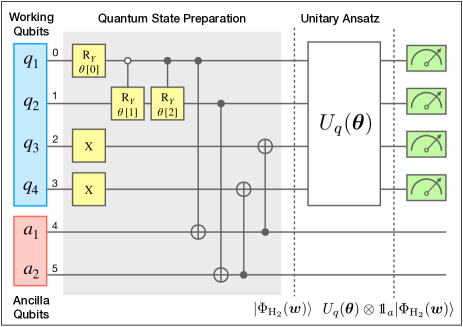
Figure 1: Sketch of the architecture of the QP-VQE algorithm implemented to compute the full spectrum of the dissociation of H₂. The first step is quantum state preparation, designed to prepare the desired state $|\Phi_{{\rm H}_{2}}(\bm{w})\rangle$. After the application of the unitary operation $U_{q}(\bm{\theta})$, a new superposition ${U_{q}(\bm{\theta})\otimes\openone_{a}\mbox{$|\Phi_{{\rm H}_{2}}(\bm{w})\rangle$}}$ is obtained. Eventually, the unitary is optimized and the eigenpairs are extracted.

IV.4 Computational cost: QP-VQE versus other known algorithms

Similar algorithms that employ the Rayleigh-Ritz variational principle have been proposed in the last years McArdle et al. (2020). Our method falls within the category of ‘weighted ensemble energy’-methods. We highlight two novel ingredients: (i) one-shot minimization of all targeted eigenenergies and (ii) a minimal number of ancilla qubits. A comparison of our method with other hybrid approaches is provided in Table 1. The most similar algorithm to QP-VQE is weighted SSVQE Nakanishi et al. (2019). It minimizes the same cost function, yet by computing each individual eigenenergy and adding them up in the classical computation. While this method does not require any ancillas, it demands $K$ times more measurements to evaluate the respective cost function (recall that $K$ is the number of targeted eigenstates). Moreover, it does not prepare a quantum state that contains information about all excited states simultaneously.

Regarding anzätze and hyperparameters $\bm{w}$, QP-VQE and SSVQE admit unitary ansätze of arbitrary complexity. In contrast, other methods suffer from an increase in computational complexity with the number of desired eigenstates Xie et al. (2022). A detailed analysis that will be presented elsewhere Ding et al. (2023) discusses the optimal choice of the QP-VQE hyperparameters $\bm{w}$. To be more specific, under the assumption that $w_{i}\neq w_{j}$ for all $i<j<K$, the sum $\sum_{j}|\varepsilon_{j}-E_{j}|$ of the absolute numerical errors of the energies of the lowest $K$ eigenstates, can be bounded by the numerical error of the value of the weighted energy

$$e_{\bm{w}}=\sum_{j=0}^{K-1}w_{j}(\varepsilon_{j}-E_{j})\,,$$ (17)

which is always positive due to the generalized variational principle Gross et al. (1988b), as follows Ding et al. (2023):

$$\sum_{j=0}^{K-1}|\varepsilon_{j}-E_{j}|\leq\frac{2\,e_{\bm{w}}}{\min_{i<j}|w_{i}-w_{j}|}\,.$$ (18)

As a result, the maximally spaced set of $\{w_{j}\}$ (in contrast to identical ones) not only reduces the upper bound of the individual energy errors, as indicated in Eq. (18), but also makes our algorithm more resilient to noise, as we will show below in Sec. VI.

The QP-VQE complexity of preparing the reference state highly depends on the problem and it is difficult to do a general comparison with other methods. Still, the examples in the next section suggest that the preparation of the reference states is likely to have lower complexity than the commonly used unitary anzätze in quantum chemistry. Another important aspect is the extraction of eigenenergies and eigenstates after optimizing the ensemble energy. By employing different weights $w_{j}$, the optimized state contains approximations of various individual eigenstates. As a direct consequence, only one Hamiltonian measurement per targeted state is needed. This is in striking contrast to democratic weighting Xu et al. (2023) which requires additional classical or quantum resources to identify in a second step the individual states within the initially targeted subspace.

In summary, QP-VQE is a resource-efficient method for excited states when computing the cost function and its gradients, which makes it suitable for near-intermediate noisy quantum (NISQ) Preskill (2018) devices in terms of run-time. Furthermore, the number of ancillas, for a fixed number of targeted states and constant ansatz complexity is the lowest possible up to the best of our knowledge Xie et al. (2022); Tilly et al. (2020); Zhang et al. (2021). The reference state preparations used in this work have at most depth $\mathcal{O}(N)$ and they are still much more shallow than the UCCGSD ansatz. QP-VQE eigenenergies and eigenstates must be extracted in an additional step that only requires $K$ Hamiltonian measurements. This extra step corresponds to a single cost function evaluation for other methods, so it becomes negligible when compared to the entire optimization procedure. Therefore QP-VQE is preferable when there are few qubits to spare and experimental run-time to save, which is the case in today’s quantum computing platforms.

		measurements
METHOD	# ancillas	cost function	$\{\varepsilon_{j}\}$ extraction
QP-VQE (this work)	$\mathcal{O}(\log_{2}K)$	$\mathcal{O}(1)$	$\mathcal{O}(K)$
SSVQE Nakanishi et al. (2019)	None	$\mathcal{O}(K)$	None
OSRVE Xie et al. (2022)	$\mathcal{O}(K)$	$\mathcal{O}(K)$	None

Table 1: Comparison of the computational costs between QP-VQE and other VQE-like methods for excited states. We estimate the resources and run-time needed for computing $K$ eigenpairs using the same unitary ansatz and the same Hamiltonian.

V Numerical experiments

In this section, we present the numerical results validating the effectiveness of our algorithm for the dissociation of H₂, LiH, and the linear H₄. All calculations were performed using the minimal STO-3G basis set. The qubit Hamiltonian was constructed using the OpenFermion McClean et al. (2017b) and OpenFermion-PySCF McClean et al. (2017b); Sun et al. (2018) plugins. Quantum simulations were conducted using PennyLane Bergholm et al. (2022) and Qiskit Qiskit contributors (2023). The optimization of circuit parameters utilized the Adam Kingma and Ba (2017) algorithm. For the calculation of the first $K$ eigenenergies, based on Eq.  18, the vector $\bm{w}$ utilized in all simulations is chosen as $(K,K-1,\cdots,1)$ and then normalized to 1. To ensure accurate results, the convergence criterion for the ensemble energy threshold was set to $10^{-9}$ Hartree. For complete access to the code and settings utilized in this work, please visit the GitHub repository git .

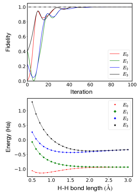
Figure 2: Computation of the spectrum of the dissociation of H₂ using QP-VQE. The upper panel illustrates the evolution of the state fidelities during the optimization process for a fixed bond length. The lower panel presents the comparison between the computed electronic eigenenergies and the exact diagonalization results (solid color line) along the dissociation path.

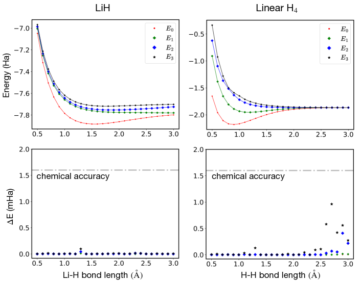
Figure 3: Ground and excited-state energies of (a) LiH and (b) Linear H₄. The lines correspond to the results obtained using the exact diagonalization method, while the dots represent our calculation using QP-VQE. Energy differences ($\Delta E=E_{\rm QP-VQE}-E_{\rm ED}$), measured in mHartree, are presented for (c) LiH and (d) Linear H₄. The dash-dot silver line represents the level of chemical accuracy.

V.1 H₂

For the H₂ molecule, which is described by 2 spatial orbitals in the STO-3G basis set, we required 4 qubits for storing the state information using JW encoding. We calculated the Qubit Hamiltonian for bond lengths ranging from 0.5 to 3.0 Å with intervals of 0.1 Å. For the H₂ molecule, we performed computations for the complete eigenspectrum within the sector $S_{z}=0$. Fig. 2 showcases the fidelity of each individual state through the optimization process. This result gives a first demonstration of the effectiveness of this approach to estimate, simultaneously, the excited states. The potential energy curves are also shown in Fig. 2. The computed results for all excited-state energies are in complete agreement with the exact diagonalization (ED) method. From the chemical perspective, it is understandable why the UCCGSD ansatz was able to generate, in this case, precise outcomes when calculating the electronic states of the hydrogen molecule in a minimal basis set. This is due to the fact that the UCCGSD ansatz considers all electronic excitations of the two electrons in the system, allowing it to exactly capture all the possible configurations of H₂. This ability of UCCGSD to expand the full Hilbert space of 2 electrons (or 2 holes) was also observed for the classical computation of the spinless Fermi-Hubbard model with five sites Benavides-Riveros et al. (2022).

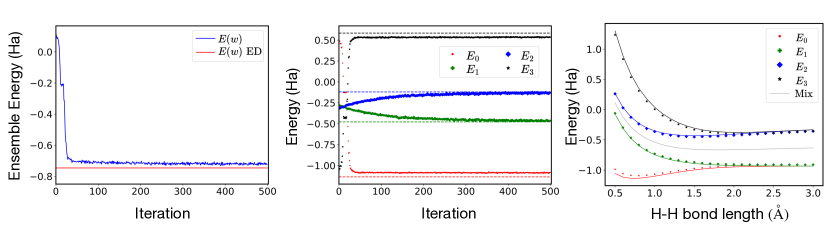
Figure 4: Left: Optimization of the ensemble energy for H-H length=0.7 Å, plotted against the exact ensemble energy (solid red line). Middle: The convergence of individual states during the optimization against the exact value (color dashed line). Right: Potential energy curves and computational errors of H₂ obtained from calculations in the presence of noise. The solid color lines depict the eigenenergies and the equiensemble energy obtained using exact diagonalization. The grey line denotes $\mbox{Tr}(H)/4$ which is the ensemble energy of a totally mixed state.

V.2 LiH

In the case of the LiH molecule, which is described by 6 spatial orbitals (12 spin-orbitals) within the STO-3G basis set, we adopt the frozen core approximation to streamline the computational process. We assume that the 1s orbital of Li is always doubly occupied and freeze it using the frozen core approximation. Accordingly, we only consider the remaining 10 spin-orbitals, which require 10 qubits using the JW encoding scheme. The potential energy curves and corresponding errors are shown in Fig. 3 (a) and (c), respectively, where the ground state ($E_{0}$) and the first three excited states ($E_{1},E_{2}$ and $E_{3}$) are calculated. As expected, the calculated results for all excited states align with the exact diagonalization method Lee et al. (2019). Moreover, the relative errors in the calculations reach chemical accuracy (1.6 mHa).

V.3 Linear H₄

Despite its simplicity, the linear H₄ system has emerged as a popular choice for investigating novel numerical approaches. With only four electrons, this system exhibits strong static electron correlations Benavides-Riveros et al. (2017), making it an ideal platform for investigating the impacts of electron interactions and benchmarking various computational methods. The outcomes of the calculations, including the ground state and the first three excited states, are illustrated in Fig. 3 (b) and (d). It is noteworthy that, based on Fig. 3 (d), higher excited states exhibit larger errors than the lower ones. This behavior can be ascribed to the enhanced complexity inherent to higher excited states, which subsequently imposes further challenges when precisely computing their energies. Also, the smaller value of the hyperparameters $w_{j}$ for higher states, which are less attended during optimization, leads to an increase in error. As the bond length increases, the states demonstrate a trend toward degeneracy. This phenomenon arises from the weakening of interatomic interactions and the gradual transformation of molecular energy levels into atomic ones. It is important to note that the final optimization result is influenced by the selection of reference states and the initial values of variational parameters. If the chosen reference states accurately capture the characteristics of the desired $K$’th excited state, the convergence to the global minimum can be achieved with fewer iterations.

VI Robustness against errors in quantum hardware

After having established the efficacy of the proposed framework in classical noiseless simulation, we proceed now to introduce noise into the simulations. To solely investigate the pure-quantum aspects of the system, we disregard the readout error. The noise model employed is based on the realistic error statistics of the ibmq$\_$manila device (see Appendix B for the comprehensive information of the device). To minimize the required number of qubits and gate operations and optimize resource utilization, we employ Checksum encoding Steudtner and Wehner (2018), instead of JW mapping. By utilizing this encoding technique, we are able to save 2 qubits for the H₂ molecule. Furthermore, we only select effective excitations (only include two independent double excitations), which reduces both the circuit depth and the number of parameters, leading to more practical computations Higgott et al. (2019); Hempel et al. (2018). In the presence of noise, we utilize the simultaneous perturbation stochastic approximation (SPSA) optimization algorithm, which is effective in situations involving measurement uncertainty on quantum computation (when finding a minimum) Kandala et al. (2017). We take $10^{4}$ measurement shots in each iteration to estimate the expectation value of the energy.

Fig. 4 shows that both the ensemble energy and individual energies exhibit convergence in the noisy simulation. We observe this trend: the ensemble energy oscillates about a stabilized average value which lies higher than the exact result. Interestingly, while the first and second excited states reach the exact value, the ground, and third excited states do not. The variational algorithm’s capability in obtaining ‘correct’ parameters McClean et al. (2016b) makes it possible for ensemble energies to stabilize at a specific level. Yet, the effect of noise (in particular, the depolarization errors prevalent in NISQ devices) may not be evenly dispersed across all individual energies. It can be observed in Fig. 4 that the ground and the first-excited energies obtained under noisy conditions are higher than the ED results. Conversely, the second and third excited state results are lower than ED, suggesting that they exhibit characteristics of a totally mixed ensemble (see gray line). We can then predict the trend of the noisy energies according to their position with respect to the totally mixed state $\mbox{Tr}(H)/4$. This fact could be exploited in the development of error mitigation techniques tailored to ensemble energies. Thus, QP-VQE shows intrinsic resilience to noise, which can be potentially improved through error mitigation.

VII Conclusions and outlook

In this work, we have presented a novel quantum parallelized variational quantum eigensolver (QP-VQE) for computing excited states which overcomes some well-known shortcomings and limitations of current hybrid quantum-classical methods. Explicitly designed to prepare eigenstates simultaneously, this variational method treats excited and ground states on the same footing by using quantum parallelism: Instead of computing $K$ eigenstates successively, QP-VQE parallelizes them and thus prepares and manipulates only one entangled state that stores all the relevant information. This simultaneous preparation of eigenstates on a quantum device offers several crucial advantages. First of all, the progressive accumulation of errors prone to schemes that calculate excited states successively is avoided. Then, using variable auxiliary weights allows one to control the error ranges of various energy levels systematically and potentially makes the algorithm more resilient to quantum noise. These unique features make QP-VQE a resource-efficient algorithm when it comes to computing the cost function and its gradients, making its future realization on noisy devices even more appealing. Finally, the simultaneous preparation of various eigenstates is conceptually appealing. In particular, it facilitates the calculation of energy gaps and transition amplitudes between eigenstates in a straightforward manner.

As a demonstration, we have conducted quantum simulations (using PennyLane and Qiskit) for several chemical systems. The computed eigenenergies and eigenstates are in excellent agreement with results from exact diagonalization. In particular, we found for all studied systems that the chosen unitary ansatz is capable of producing both ground and excited states with roughly the same quality. Furthermore, in the presence of gate errors, yet without error mitigation, the minimization procedure still yields decent results. Thus we expect that in more sophisticated implementations of QP-VQE where all available error mitigation techniques are applied Lolur et al. (2023); van den Berg et al. (2022, 2023); Temme et al. (2017), QP-VQE can reach ranges of numerical accuracy comparable to other state-of-the-art methods from quantum computing.

The evidence we provided for the effectiveness of QP-VQE from both a conceptual and computational point of view encourages further explorations in several directions. For instance, the algorithm can be implemented in combination with a wide range of existing numerical methods. Just to give an example, a neural network can be trained to learn the parameters of a quantum circuit preparing thus not only a chemical ground state as in Refs. Ceroni et al. (2023); Shang et al. (2023) but also the quantum parallelized state that encodes various eigenstates. Similarly, since the parallelization technique we have proposed is indifferent to the quantum statistics of the underlying problem, our algorithm can also potentially be applied to study vibrational spectra which could have a tremendous impact on the long-sought full quantum treatment of Fermi-Bose mixtures Fregoni et al. (2022); Marini (2023); Basov et al. (2021).

Appendix A Quantum state preparation for the H₂ molecule

To prepare the quantum state in Eq. 14, we first construct the compressed state on the first two qubits ($q_{1}$, $q_{2}$) with the desired weights $w_{0},w_{1},..$. A simple rotation (control-rotation) achieves this. Indeed, note that we need $3$ rotation angles to perform all possible 4-dimensional real vectors $\bm{w}$. If, in addition, we impose the decreasing order $w_{j}>w_{j+1}$, we can reduce the circuit and rotation angles we used. The preparation of the compressed state is the following:

$$|0_{q_{1}}0_{q_{2}}\rangle \xrightarrow[]{R_{y}}\cos{\frac{\theta_{0}}{2}}\mbox{$|0_{q_{1}}0_{q_{2}}\rangle$}+\sin{\frac{\theta_{0}}{2}}\mbox{$|1_{q_{1}}0_{q_{2}}\rangle$}$$

$$\xrightarrow[]{C_{0}R_{y}}\cos{\frac{\theta_{0}}{2}}\cos{\frac{\theta_{1}}{2}}\mbox{$|0_{q_{1}}0_{q_{2}}\rangle$}+\cos{\frac{\theta_{0}}{2}}\sin{\frac{\theta_{1}}{2}}\mbox{$|0_{q_{1}}1_{q_{2}}\rangle$}+\sin{\frac{\theta_{0}}{2}}\mbox{$|1_{q_{1}}0_{q_{2}}\rangle$}$$

$$\xrightarrow[]{C_{1}R_{y}}\cos{\frac{\theta_{0}}{2}}\cos{\frac{\theta_{1}}{2}}\mbox{$|0_{q_{1}}0_{q_{2}}\rangle$}+\cos{\frac{\theta_{0}}{2}}\sin{\frac{\theta_{1}}{2}}\mbox{$|0_{q_{1}}1_{q_{2}}\rangle$}+\sin{\frac{\theta_{0}}{2}}\cos{\frac{\theta_{2}}{2}}\mbox{$|1_{q_{1}}0_{q_{2}}\rangle$}+\sin{\frac{\theta_{0}}{2}}\sin{\frac{\theta_{2}}{2}}\mbox{$|1_{q_{1}}1_{q_{2}}\rangle$}$$

$$=\sqrt{w_{0}}\mbox{$|0_{q_{1}}0_{q_{2}}\rangle$}+\sqrt{w_{1}}\mbox{$|0_{q_{1}}1_{q_{2}}\rangle$}+\sqrt{w_{2}}\mbox{$|1_{q_{1}}0_{q_{2}}\rangle$}+\sqrt{w_{3}}\mbox{$|1_{q_{1}}1_{q_{2}}\rangle$}\,.$$

Next, one can map it back to our desired state 14 using an X and CNOT gates, as indicated in Fig. 1. Assuming all other qubits ($q_{2}$,$q_{3}$,$a_{0}$,$a_{1}$) are initialized to $0$ we have:

$$\sqrt{w_{0}}\mbox{$|0_{q_{1}}0_{q_{2}}\rangle$}+\sqrt{w_{1}}\mbox{$|0_{q_{1}}1_{q_{2}}\rangle$}+\sqrt{w_{2}}\mbox{$|1_{q_{1}}0_{q_{2}}\rangle$}+\sqrt{w_{3}}\mbox{$|1_{q_{1}}1_{q_{2}}\rangle$}$$

$$\qquad\,\,\xrightarrow[]{X_{q_{3}}X_{q_{4}}}\sqrt{w_{0}}\mbox{$|0_{q_{1}}0_{q_{2}}1_{q_{3}}1_{q_{4}}\rangle$}+\sqrt{w_{1}}\mbox{$|0_{q_{1}}1_{q_{2}}1_{q_{3}}1_{q_{4}}\rangle$}+\sqrt{w_{2}}\mbox{$|1_{q_{1}}0_{q_{2}}1_{q_{3}}1_{q_{4}}\rangle$}+\sqrt{w_{3}}\mbox{$|1_{q_{1}}1_{q_{2}}1_{q_{3}}1_{q_{4}}\rangle$}$$

$$\xrightarrow[{\rm C}_{1}{\rm NOT}(q_{1},a_{1})]{{\rm C}_{1}{\rm NOT}(q_{2},a_{2})}\sqrt{w_{0}}\mbox{$|0_{q_{1}}0_{q_{2}}1_{q_{3}}1_{q_{4}}0_{a_{1}}0_{a_{2}}\rangle$}+\sqrt{w_{1}}\mbox{$|0_{q_{1}}1_{q_{2}}1_{q_{3}}1_{q_{4}}0_{a_{1}}1_{a_{2}}\rangle$}+\sqrt{w_{2}}\mbox{$|1_{q_{1}}0_{q_{2}}1_{q_{3}}1_{q_{4}}1_{a_{1}}0_{a_{2}}\rangle$}+\sqrt{w_{3}}\mbox{$|1_{q_{1}}1_{q_{2}}1_{q_{3}}1_{q_{4}}1_{a_{1}}1_{a_{2}}\rangle$}$$

$$\xrightarrow[{\rm C}_{1}{\rm NOT}(a_{2},q_{4})]{{\rm C}_{1}{\rm NOT}(a_{1},q_{3})}\sqrt{w_{0}}\mbox{$|0_{q_{1}}0_{q_{2}}1_{q_{3}}1_{q_{4}}0_{a_{1}}0_{a_{2}}\rangle$}+\sqrt{w_{1}}\mbox{$|0_{q_{1}}1_{q_{2}}1_{q_{3}}0_{q_{4}}0_{a_{1}}1_{a_{2}}\rangle$}+\sqrt{w_{2}}\mbox{$|1_{q_{1}}0_{q_{2}}0_{q_{3}}1_{q_{4}}1_{a_{1}}0_{a_{2}}\rangle$}+\sqrt{w_{3}}\mbox{$|1_{q_{1}}1_{q_{2}}0_{q_{3}}0_{q_{4}}1_{a_{1}}1_{a_{2}}\rangle$}$$

$$\qquad\,\,\xrightarrow[]{\text{Reorder}}\sqrt{w_{0}}\mbox{$|1100\rangle$}_{q}\mbox{$|00\rangle$}_{a}+\sqrt{w_{1}}\mbox{$|1001\rangle$}_{q}\mbox{$|01\rangle$}_{a}+\sqrt{w_{2}}\mbox{$|0110\rangle$}_{q}\mbox{$|10\rangle$}_{a}+\sqrt{w_{3}}\mbox{$|0011\rangle$}_{q}\mbox{$|11\rangle$}_{a}=\mbox{$|\Phi_{{\rm H}_{2}}(\bm{w})\rangle$}\,,$$

which is the initial state (14).

Appendix B Calibration of the IBMQ MANILA quantum computer

In this section, we present the parameters of the error model used for running the noisy simulations (see Table 2). They were extracted from the ibmq$\_$manila noise model of the Aer Simulator. All the calibration data also can be found in Ref. git .

Qubit	$Q_{0}$	$Q_{1}$	$Q_{2}$	$Q_{3}$	$Q_{4}$
$T_{1}$ in $\mu s$	20.931	145.271	74.739	188.731	138.941
$T_{2}$ in $\mu s$	18.130	63.372	17.264	60.765	37.822
Frequency in GHz	4.962	4.838	5.037	4.951	5.065
Anharmonicity in GHz	-0.34463	-0.34528	-0.34255	-0.34358	-0.34211
SPAM error $\mbox{$|1\rangle$}\rightarrow\mbox{$|0\rangle$}$	0.0574	0.0556	0.0338	0.0384	0.034
SPAM error $\mbox{$|0\rangle$}\rightarrow\mbox{$|1\rangle$}$	0.016	0.0134	0.0198	0.0106	0.0100
Identity,$\sqrt{X}$, X errors ($\times 10^{4}$)	6.2809	2.1191	2.5059	2.0525	3.8590
CNOT error	0 $\leftrightarrow$ 1: 0.0076	1 $\leftrightarrow$ 2 : 0.04386	2 $\leftrightarrow$ 3 : 0.03558	3 $\leftrightarrow$ 4 : 0.00628
CNOT Gate time in ns	277.333	469.333	355.556	334.222

Table 2: Calibration used for the ibmq$\_$manila quantum computer.

Appendix C Measuring observables directly in the ensemble state

As explained in Sec. IV.3, once the optimization procedure is finished, we get a unitary $U$ that produces the $K$ low-lying states such that $|\varepsilon_{i}\rangle=U|\phi_{i}\rangle$ with $i=0,...,K-1$. After preparing each state $|\varepsilon_{i}\rangle$ we can calculate any observable, e.g., the energies result from $\varepsilon_{i}=\langle\varepsilon_{i}|\hat{H}|\varepsilon_{i}\rangle$. However, there is a second approach to the computation of relevant quantities that utilizes quantum parallelism. To give an example, let us prepare the following state in the quantum register:

$$|\Psi\rangle=\dfrac{1}{\sqrt{2}}\left(|\varepsilon_{0}\rangle_{q}|0\rangle_{a}+|\varepsilon_{1}\rangle_{q}|1\rangle_{a}\right).$$ (19)

Preparing this state can be done using techniques similar to the ones shown in the main text. We need only one additional ancilla qubit and, by selecting the reference states $|\phi_{i}\rangle$, we can target any gap in the sup-space we work on. Then we get the energy gap $\varepsilon_{0}-\varepsilon_{1}$ by computing the expectation value of the operator $\hat{H_{q}}\otimes\hat{Z_{a}}$:

$$\langle\Psi|\hat{H_{q}}\otimes\hat{Z_{a}}|\Psi\rangle=\dfrac{\varepsilon_{0}-\varepsilon_{1}}{2}.$$ (20)

This allows us to compute energy gaps with only one Hamiltonian measurement instead of two. The generalization to arbitrary states is straightforward. For instance, in the case of the H₂ molecule, whose final state reads:

$$\mbox{$|\Psi_{{\rm H}_{2}}\rangle$}=\dfrac{1}{2}\left(|\varepsilon_{0}\rangle_{q}|00\rangle_{a}+|\varepsilon_{1}\rangle_{q}|10\rangle_{a}+|\varepsilon_{2}\rangle_{q}|01\rangle_{a}+|\varepsilon_{3}\rangle_{q}|11\rangle_{a}\right)\,,$$ (21)

the energy gap $\varepsilon_{0}-\varepsilon_{1}$ can be computed by means of the expectation value of the operator $\hat{H_{q}}\otimes(\hat{Z}\otimes\tfrac{1}{2}(\openone+\hat{Z}))_{a}$. Similarly, the gaps $\varepsilon_{2}-\varepsilon_{3}$ and $\varepsilon_{0}-\varepsilon_{2}$ can be computed using the operators $\hat{H_{q}}\otimes(\hat{Z}\otimes\tfrac{1}{2}(\openone-\hat{Z}))_{a}$ and $\hat{H_{q}}\otimes(\tfrac{1}{2}(\openone+\hat{Z})\otimes\hat{Z})_{a}$, respectively.

A similar procedure can also give other non-diagonal quantities, such as the molecular dipole moment transition amplitudes. In that case, one needs to compute the expectation value of the operator $\hat{\mathbf{d}_{q}}\otimes\hat{X_{a}}$, where $\hat{\mathbf{d}}$ is the dipole moment operator, with the state (19):

$$\langle\Psi|\hat{\mathbf{d}_{q}}\otimes\hat{X_{a}}|\Psi\rangle=\frac{\mbox{$\langle\varepsilon_{1}|$}\hat{\mathbf{d}}|\varepsilon_{0}\rangle+\mbox{$\langle\varepsilon_{0}|$}\hat{\mathbf{d}}|\varepsilon_{1}\rangle}{2}\,.$$ (22)

Notice that computing the expectation value of operators of the form $\hat{\mathbf{d}_{q}}\otimes(\hat{X}\otimes\tfrac{1}{2}(\openone\pm\hat{Z}))_{a}$ and $\hat{\mathbf{d}_{q}}\otimes(\tfrac{1}{2}(\openone\pm\hat{Z})\otimes\hat{X})_{a}$ with the state $|\Psi_{{\rm H}_{2}}\rangle$ gives transition amplitudes of the eigenstates of H₂.

These examples illustrate the ability of ensemble states to reduce run-time overhead in the computation of observables.

References

- González et al. (2012) L. González, D. Escudero, and L. Serrano-Andrés, “Progress and Challenges in the Calculation of Electronic Excited States,” ChemPhysChem 13, 28 (2012).
- Onida et al. (2002) G. Onida, L. Reining, and A. Rubio, “Electronic excitations: density-functional versus many-body Green’s-function approaches,” Rev. Mod. Phys. 74, 601 (2002).
- Serrano-Andrés and Merchán (2005) L. Serrano-Andrés and M. Merchán, “Quantum chemistry of the excited state: 2005 overview,” J. Mol. Struct.: THEOCHEM 729, 99 (2005).
- Westermayr and Marquetand (2021) J. Westermayr and P. Marquetand, “Machine Learning for Electronically Excited States of Molecules,” Chem. Rev. 121, 9873 (2021).
- Loos et al. (2018) P.-F. Loos, A. Scemama, A. Blondel, Y. Garniron, M. Caffarel, and D. Jacquemin, “A Mountaineering Strategy to Excited States: Highly Accurate Reference Energies and Benchmarks,” J. Chem. Theory Comput. 14, 4360 (2018).
- Ghosh et al. (2018) S. Ghosh, P. Verma, C. J. Cramer, L. Gagliardi, and D. G. Truhlar, “Combining Wave Function Methods with Density Functional Theory for Excited States,” Chem. Rev. 118, 7249 (2018).
- González and Lindh (2020) L. González and R. Lindh, eds., Quantum Chemistry and Dynamics of Excited States: Methods and Applications (John Wiley & Sons, Ltd, 2020).
- Cirac and Zoller (2012) J. I. Cirac and P. Zoller, “Goals and opportunities in quantum simulation,” Nature Phys. 8, 264–266 (2012).
- Preskill (2018) J. Preskill, “Quantum Computing in the NISQ era and beyond,” Quantum 2, 79 (2018).
- Xie et al. (2022) Q.-X. Xie, S Liu, and Y. Zhao, “Orthogonal State Reduction Variational Eigensolver for the Excited-State Calculations on Quantum Computers,” J. Chem. Theory Comput. 18, 3737 (2022).
- Parrish et al. (2019) R. M. Parrish, E. G. Hohenstein, P. L. McMahon, and T. J. Martínez, “Quantum Computation of Electronic Transitions Using a Variational Quantum Eigensolver,” Phys. Rev. Lett. 122, 230401 (2019).
- Ollitrault et al. (2020) P. J. Ollitrault, A. Kandala, C.-F. Chen, P. Kl. Barkoutsos, A. Mezzacapo, M. Pistoia, S. Sheldon, S. Woerner, J. M. Gambetta, and I. Tavernelli, “Quantum equation of motion for computing molecular excitation energies on a noisy quantum processor,” Phys. Rev. Res. 2, 043140 (2020).
- Lyu et al. (2023) C. Lyu, X. Xu, M.-H. Yung, and A. Bayat, “Symmetry enhanced variational quantum spin eigensolver,” Quantum 7, 899 (2023).
- Colless et al. (2018) J. I. Colless, V. V. Ramasesh, D. Dahlen, M. S. Blok, M. E. Kimchi-Schwartz, J. R. McClean, J. Carter, W. A. de Jong, and I. Siddiqi, “Computation of Molecular Spectra on a Quantum Processor with an Error-Resilient Algorithm,” Phys. Rev. X 8, 011021 (2018).
- Gocho et al. (2023) S. Gocho, H. Nakamura, S. Kanno, Q. Gao, T. Kobayashi, T. Inagaki, and M. Hatanaka, “Excited state calculations using variational quantum eigensolver with spin-restricted ansätze and automatically-adjusted constraints,” npj Comput. Mater. 9, 13 (2023).
- Tazi and Thom (2023) L. C. Tazi and A. J. W. Thom, “Folded Spectrum VQE: A quantum computing method for the calculation of molecular excited states,” (2023), arXiv:2305.04783 .
- Head-Marsden et al. (2021) K. Head-Marsden, J. Flick, C. J. Ciccarino, and P. Narang, “Quantum Information and Algorithms for Correlated Quantum Matter,” Chem. Rev. 121, 3061–3120 (2021).
- Peruzzo et al. (2014) A. Peruzzo, J. McClean, P. Shadbolt, M.-H. Yung, X.-Q. Zhou, P. J. Love, A. Aspuru-Guzik, and J. L. O’Brien, “A variational eigenvalue solver on a photonic quantum processor,” Nat. Comm. 5, 4213 (2014).
- McClean et al. (2016a) J. R. McClean, J. Romero, R. Babbush, and A. Aspuru-Guzik, “The theory of variational hybrid quantum-classical algorithms,” New J. Phys. 18, 023023 (2016a).
- Fedorov et al. (2022) D. A. Fedorov, B. Peng, N. Govind, and Y. Alexeev, “VQE method: a short survey and recent developments,” Mater. Theory 6, 2 (2022).
- Cao et al. (2019) Y. Cao, J. Romero, J. P. Olson, M. Degroote, P. D. Johnson, M. Kieferová, I. D. Kivlichan, T. Menke, B. Peropadre, N. P. D. Sawaya, S. Sim, L. Veis, and A. Aspuru-Guzik, “Quantum Chemistry in the Age of Quantum Computing,” Chem. Rev. 119, 10856 (2019).
- Santagati et al. (2018) R. Santagati, J. Wang, A. A. Gentile, S. Paesani, N. Wiebe, J. R. McClean, S. Morley-Short, P. J. Shadbolt, D. Bonneau, J. W. Silverstone, D. P. Tew, X. Zhou, J. L. O’Brien, and G. Thompson M, “Witnessing eigenstates for quantum simulation of Hamiltonian spectra,” Sci. Adv. 4, eaap9646 (2018).
- McArdle et al. (2020) S. McArdle, S. Endo, A. Aspuru-Guzik, S. C. Benjamin, and X. Yuan, “Quantum computational chemistry,” Rev. Mod. Phys. 92, 015003 (2020).
- McClean et al. (2017a) J. R. McClean, M. E. Kimchi-Schwartz, J. Carter, and W. A. de Jong, “Hybrid quantum-classical hierarchy for mitigation of decoherence and determination of excited states,” Phys. Rev. A 95, 042308 (2017a).
- Zhang et al. (2022) D.-B. Zhang, B.-L. Chen, Z.-H. Yuan, and T. Yin, “Variational quantum eigensolvers by variance minimization,” Chin. Phys. B 31, 120301 (2022).
- Wang and Mazziotti (2023) Y. Wang and D. A. Mazziotti, “Electronic Excited States from a Variance-Based Contracted Quantum Eigensolver,” (2023), arXiv:2305.03044 .
- Higgott et al. (2019) O. Higgott, D. Wang, and S. Brierley, “Variational Quantum Computation of Excited States,” Quantum 3, 156 (2019).
- Jones et al. (2019) T. Jones, S. Endo, S. McArdle, X. Yuan, and S. C. Benjamin, “Variational quantum algorithms for discovering Hamiltonian spectra,” Phys. Rev. A 99, 062304 (2019).
- Ibe et al. (2022) Y. Ibe, Y. O. Nakagawa, N. Earnest, T. Yamamoto, K. Mitarai, Q. Gao, and T. Kobayashi, “Calculating transition amplitudes by variational quantum deflation,” Phys. Rev. Res. 4, 013173 (2022).
- Wen et al. (2021) J. Wen, D. Lv, M.-H. Yung, and G.-L. Long, “Variational quantum packaged deflation for arbitrary excited states,” Quantum Eng. 3, e80 (2021).
- Shirai et al. (2022) S. Shirai, T. Horiba, and H. Hirai, “Calculation of Core-Excited and Core-Ionized States Using Variational Quantum Deflation Method and Applications to Photocatalyst Modeling,” ACS Omega 7, 10840 (2022).
- Nakanishi et al. (2019) K. M. Nakanishi, K. Mitarai, and K. Fujii, “Subspace-search variational quantum eigensolver for excited states,” Phys. Rev. Res. 1, 033062 (2019).
- Yalouz et al. (2021) S. Yalouz, B. Senjean, J. Günther, F. Buda, T. O’Brien, and L. Visscher, “A state-averaged orbital-optimized hybrid quantum–classical algorithm for a democratic description of ground and excited states,” Quantum Sci. Technol. 6, 024004 (2021).
- Kuroiwa and Nakagawa (2021) K. Kuroiwa and Y. O. Nakagawa, “Penalty methods for a variational quantum eigensolver,” Phys. Rev. Res. 3, 013197 (2021).
- Xu et al. (2023) G. Xu, Y. B. Guo, X. Li, K. Wang, Z. Fan, Z. S. Zhou, H. J. Liao, and T. Xiang, “Concurrent quantum eigensolver for multiple low-energy eigenstates,” Phys. Rev. A 107, 052423 (2023).
- Gross et al. (1988a) E. K. U. Gross, L. N. Oliveira, and W. Kohn, “Density-functional theory for ensembles of fractionally occupied states. I. Basic formalism,” Phys. Rev. A 37, 2809 (1988a).
- Fromager (2020) E. Fromager, “Individual Correlations in Ensemble Density Functional Theory: State- and Density-Driven Decompositions without Additional Kohn-Sham Systems,” Phys. Rev. Lett. 124, 243001 (2020).
- Schilling and Pittalis (2021) C. Schilling and S. Pittalis, “Ensemble Reduced Density Matrix Functional Theory for Excited States and Hierarchical Generalization of Pauli’s Exclusion Principle,” Phys. Rev. Lett. 127, 023001 (2021).
- Liebert et al. (2022) J. Liebert, F. Castillo, J.-P. Labbé, and C. Schilling, “Foundation of one-particle reduced density matrix functional theory for excited states,” J. Chem. Theory Comput. 18, 124 (2022).
- Gould et al. (2023) T. Gould, D. P. Kooi, P. Gori-Giorgi, and S. Pittalis, “Electronic Excited States in Extreme Limits via Ensemble Density Functionals,” Phys. Rev. Lett. 130, 106401 (2023).
- Liebert and Schilling (2023) J. Liebert and C. Schilling, “An exact one-particle theory of bosonic excitations: from a generalized Hohenberg–Kohn theorem to convexified N-representability,” New J. Phys. 25, 013009 (2023).
- Cernatic et al. (2021) F. Cernatic, B. Senjean, V. Robert, and E. Fromager, “Ensemble Density Functional Theory of Neutral and Charged Excitations,” Top. Curr. Chem. 380, 4 (2021).
- Ding et al. (2023) L. Ding, C. L. Benavides-Riveros, and C. Schilling, “in preparation,” (2023).
- Seki et al. (2020) K. Seki, T. Shirakawa, and S. Yunoki, “Symmetry-adapted variational quantum eigensolver,” Phys. Rev. A 101, 052340 (2020).
- Lyu et al. (2020) C. Lyu, V. Montenegro, and A. Bayat, “Accelerated variational algorithms for digital quantum simulation of many-body ground states,” Quantum 4, 324 (2020).
- Ryabinkin et al. (2019) I. G. Ryabinkin, S. N. Genin, and A. F. Izmaylov, “Constrained Variational Quantum Eigensolver: Quantum Computer Search Engine in the Fock Space,” J. Chem. Theory Comput. 15, 249 (2019).
- Israel (1976) W. Israel, “Thermo-field dynamics of black holes,” Phys. Lett. A 57, 107 (1976).
- Takahashi and Umezawa (1996) Y. Takahashi and H. Umezawa, “Thermo field dynamics,” Int. J. Mod. Phys. B 10, 1755 (1996).
- Borrelli and Gelin (2021) R. Borrelli and M. F. Gelin, “Finite temperature quantum dynamics of complex systems: Integrating thermo-field theories and tensor-train methods,” WIREs Comput. Mol. Sci. 11, e1539 (2021).
- Benavides-Riveros et al. (2022) C. L. Benavides-Riveros, L. Chen, C. Schilling, S. Mantilla, and S. Pittalis, “Excitations of Quantum Many-Body Systems via Purified Ensembles: A Unitary-Coupled-Cluster-Based Approach,” Phys. Rev. Lett. 129, 066401 (2022).
- Pollmann et al. (2016) F. Pollmann, V. Khemani, J. I. Cirac, and S. L. Sondhi, “Efficient variational diagonalization of fully many-body localized Hamiltonians,” Phys. Rev. B 94, 041116 (2016).
- Sagastizabal et al. (2021) R. Sagastizabal, S. P. Premaratne, B. A. Klaver, M. A. Rol, V. Negîrneac, M. S. Moreira, X. Zou, S. Johri, N. Muthusubramanian, M. Beekman, C. Zachariadis, V. P. Ostroukh, N. Haider, A. Bruno, A. Y. Matsuura, and L. DiCarlo, “Variational preparation of finite-temperature states on a quantum computer,” npj Quantum Inf. 7, 130 (2021).
- Sager and Mazziotti (2022) L. M. Sager and D. A. Mazziotti, “Cooper-pair condensates with nonclassical long-range order on quantum devices,” Phys. Rev. Res. 4, 013003 (2022).
- Wu and Hsieh (2019) J. Wu and T. H. Hsieh, “Variational Thermal Quantum Simulation via Thermofield Double States,” Phys. Rev. Lett. 123, 220502 (2019).
- Khamoshi et al. (2022) A. Khamoshi, G. P. Chen, F. A. Evangelista, and G. E. Scuseria, “AGP-based unitary coupled cluster theory for quantum computers,” Quantum Sci. Technol. 8, 015006 (2022).
- Jiménez-Hoyos et al. (2012) C. A. Jiménez-Hoyos, T. M. Henderson, T. Tsuchimochi, and G. E. Scuseria, “Projected Hartree–Fock theory,” J. Chem. Phys. 136, 164109 (2012).
- Khamoshi et al. (2023) A. Khamoshi, R. Dutta, and G. E. Scuseria, “State Preparation of Antisymmetrized Geminal Power on a Quantum Computer without Number Projection,” J. Phys. Chem. A 127, 4005 (2023).
- Jordan and Wigner (1928) P. Jordan and E. Wigner, “Über das paulische Äquivalenzverbot,” Z. Physik 47, 631 (1928).
- Mottonen et al. (2004) M. Mottonen, J. Vartiainen, V. Bergholm, and M. Salomaa, “Transformation of quantum states using uniformly controlled rotations,” (2004), arXiv:quant-ph/0407010 .
- Tubman et al. (2018) N. M. Tubman, C. Mejuto-Zaera, J. M. Epstein, D. Hait, D. S. Levine, W. Huggins, Z. Jiang, J. R. McClean, R. Babbush, M. Head-Gordon, and K. B. Whaley, “Postponing the orthogonality catastrophe: efficient state preparation for electronic structure simulations on quantum devices,” (2018), arXiv:1809.05523 .
- Araujo et al. (2021) I. F. Araujo, D. K. Park, F. Petruccione, and A. J. da Silva, “A divide-and-conquer algorithm for quantum state preparation,” Sci. Rep. 11, 6329 (2021).
- Arrazola et al. (2022) J. M. Arrazola, O. Di Matteo, N. Quesada, S. Jahangiri, A. Delgado, and N. Killoran, “Universal quantum circuits for quantum chemistry,” Quantum 6, 742 (2022).
- Shende et al. (2006) V. V. Shende, S. S. Bullock, and I. L. Markov, “Synthesis of quantum-logic circuits,” IEEE Trans. Comput.-Aided Des. Integr. Circuits Syst. 25, 1000 (2006).
- Childs et al. (2018) A. M. Childs, D. Maslov, Y. Nam, N. J. Ross, and Y. Su, “Toward the first quantum simulation with quantum speedup,” Proc. Natl. Acad. Sci. U.S.A. 115, 9456 (2018).
- Babbush et al. (2018) R. Babbush, C. Gidney, D. W. Berry, N. Wiebe, J. McClean, A. Paler, A. Fowler, and H. Neven, “Encoding Electronic Spectra in Quantum Circuits with Linear T Complexity,” Phys. Rev. X 8, 041015 (2018).
- Romero et al. (2018a) J. Romero, R. Babbush, J. R. McClean, C. Hempel, P. J. Love, and A. Aspuru-Guzik, “Strategies for quantum computing molecular energies using the unitary coupled cluster ansatz,” Quantum Sci. and Technol. 4, 014008 (2018a).
- Lee et al. (2019) J. Lee, W. J. Huggins, M. Head-Gordon, and K. B. Whaley, “Generalized Unitary Coupled Cluster Wave functions for Quantum Computation,” J. Chem. Theory Comput. 15, 311 (2019).
- Nooijen (2000) M. Nooijen, “Can the Eigenstates of a Many-Body Hamiltonian Be Represented Exactly Using a General Two-Body Cluster Expansion?” Phys. Rev. Lett. 84, 2108 (2000).
- Grimsley et al. (2019) H. R. Grimsley, S. E. Economou, E. Barnes, and N. J. Mayhall, “An adaptive variational algorithm for exact molecular simulations on a quantum computer,” Nat. Commun. 10, 3007 (2019).
- Kandala et al. (2017) A. Kandala, A. Mezzacapo, K. Temme, M. Takita, M. Brink, J. M. Chow, and J. M. Gambetta, “Hardware-efficient variational quantum eigensolver for small molecules and quantum magnets,” Nature 549, 242 (2017).
- Anand et al. (2022) A. Anand, P. Schleich, S. Alperin-Lea, P. W. K. Jensen, S. Sim, M. Díaz-Tinoco, J. S. Kottmann, M. Degroote, A. F. Izmaylov, and A. Aspuru-Guzik, “A quantum computing view on unitary coupled cluster theory,” Chem. Soc. Rev. 51, 1659 (2022).
- Wecker et al. (2015) D. Wecker, M. B. Hastings, and M. Troyer, “Progress towards practical quantum variational algorithms,” Phys. Rev. A 92, 042303 (2015).
- Greene-Diniz and Muñoz Ramo (2021) G. Greene-Diniz and D. Muñoz Ramo, “Generalized unitary coupled cluster excitations for multireference molecular states optimized by the variational quantum eigensolver,” Int. J. Quantum Chem. 121, e26352 (2021).
- Chan et al. (2021) H. Chan, N. Fitzpatrick, J. Segarra-Martí, M. Bearpark, and D. Tew, “Molecular excited state calculations with adaptive wavefunctions on a quantum eigensolver emulation: reducing circuit depth and separating spin states,” Phys. Chem. Chem. Phys. 23, 26438 (2021).
- Romero et al. (2018b) J. Romero, R. Babbush, J. R. McClean, C. Hempel, P. J. Love, and A. Aspuru-Guzik, “Strategies for quantum computing molecular energies using the unitary coupled cluster ansatz,” Quantum Sci. Technol. 4, 014008 (2018b).
- Barkoutsos et al. (2018) P. Barkoutsos, J. F. Gonthier, I. Sokolov, N. Moll, G. Salis, A. Fuhrer, M. Ganzhorn, D. J. Egger, M. Troyer, A. Mezzacapo, S. Filipp, and I. Tavernelli, “Quantum algorithms for electronic structure calculations: Particle-hole Hamiltonian and optimized wave-function expansions,” Phys. Rev. A 98, 022322 (2018).
- Gross et al. (1988b) E. K. U. Gross, L. N. Oliveira, and W. Kohn, “Rayleigh-ritz variational principle for ensembles of fractionally occupied states,” Phys. Rev. A 37, 2805–2808 (1988b).
- Tilly et al. (2020) J. Tilly, G. Jones, H. Chen, L. Wossnig, and E. Grant, “Computation of molecular excited states on IBM quantum computers using a discriminative variational quantum eigensolver,” Phys. Rev. A 102, 062425 (2020).
- Zhang et al. (2021) F. Zhang, N. Gomes, Y. Yao, P. P. Orth, and T. Iadecola, “Adaptive variational quantum eigensolvers for highly excited states,” Phys. Rev. B 104, 075159 (2021).
- McClean et al. (2017b) J. McClean et al., “OpenFermion: the electronic structure package for quantum computers,” Quantum Sci. and Technol. 5, 034014 (2017b).
- Sun et al. (2018) Q. Sun, T. C. Berkelbach, N. S. Blunt, G. H. Booth, S. Guo, Z. Li, J. Liu, J. D. McClain, E. R. Sayfutyarova, S. Sharma, S. Wouters, and G. K.-L. Chan, “PySCF: the Python-based simulations of chemistry framework,” WIREs Comput. Mol. Sci. 8, e1340 (2018).
- Bergholm et al. (2022) V. Bergholm et al., “PennyLane: Automatic differentiation of hybrid quantum-classical computations,” (2022), arXiv:1811.04968 .
- Qiskit contributors (2023) Qiskit contributors, “Qiskit: An open-source framework for quantum computing,” (2023).
- Kingma and Ba (2017) D. P. Kingma and J. Ba, “Adam: A Method for Stochastic Optimization,” (2017), arXiv:1412.6980 .
- (85) https://github.com/x0-chenglin/PVQE.
- Benavides-Riveros et al. (2017) C. L. Benavides-Riveros, N. N. Lathiotakis, and M. A. L. Marques, “Towards a formal definition of static and dynamic electronic correlations,” Phys. Chem. Chem. Phys. 19, 12655 (2017).
- Steudtner and Wehner (2018) M. Steudtner and S. Wehner, “Fermion-to-qubit mappings with varying resource requirements for quantum simulation,” New J. Phys. 20, 063010 (2018).
- Hempel et al. (2018) C. Hempel, C. Maier, J. Romero, J. McClean, T. Monz, H. Shen, P. Jurcevic, B. P. Lanyon, P. Love, Ryan Babbush, A. Aspuru-Guzik, R. Blatt, and C. F. Roos, “Quantum Chemistry Calculations on a Trapped-Ion Quantum Simulator,” Phys. Rev. X 8, 031022 (2018).
- McClean et al. (2016b) J. McClean, J. Romero, R. Babbush, and A. Aspuru-Guzik, “The theory of variational hybrid quantum-classical algorithms,” New J. Phys. 18, 023023 (2016b).
- Lolur et al. (2023) P. Lolur et al., “Reference-State Error Mitigation: A Strategy for High Accuracy Quantum Computation of Chemistry,” J. Chem. Theory Comput. 19, 783 (2023).
- van den Berg et al. (2022) E. van den Berg, Z. K. Minev, and K. Temme, “Model-free readout-error mitigation for quantum expectation values,” Phys. Rev. A 105, 032620 (2022).
- van den Berg et al. (2023) E. van den Berg, Z. Minev, A. Kandala, and K. Temme, “Probabilistic error cancellation with sparse Pauli–Lindblad models on noisy quantum processors,” Nat. Phys. (2023), 10.1038/s41567-023-02042-2.
- Temme et al. (2017) K. Temme, S. Bravyi, and J. M. Gambetta, “Error Mitigation for Short-Depth Quantum Circuits,” Phys. Rev. Lett. 119, 180509 (2017).
- Ceroni et al. (2023) J. Ceroni, T. F. Stetina, M. Kieferova, C. O. Marrero, J. M. Arrazola, and N. Wiebe, “Generating Approximate Ground States of Molecules Using Quantum Machine Learning,” (2023), arXiv:2210.05489 [quant-ph] .
- Shang et al. (2023) H. Shang, Y. Fan, L. Shen, C. Guo, J. Liu, X. Duan, F. Li, and Z. Li, “Towards practical and massively parallel quantum computing emulation for quantum chemistry,” npj Quantum Inf. 9, 33 (2023).
- Fregoni et al. (2022) J. Fregoni, F. J. Garcia-Vidal, and J. Feist, “Theoretical Challenges in Polaritonic Chemistry,” ACS Photonics 9, 1096 (2022).
- Marini (2023) A. Marini, “Equilibrium and out-of-equilibrium realistic phonon self-energy free from overscreening,” Phys. Rev. B 107, 024305 (2023).
- Basov et al. (2021) D. N. Basov, A. Asenjo-Garcia, P. J. Schuck, X. Zhu, and A. Rubio, “Polariton panorama,” Nanophotonics 10, 549 (2021).