On Compositionality and Improved Training of NADO

Abstract

NeurAlly-Decomposed Oracle (NADO) is a powerful approach for controllable generation with large language models. Differentiating from finetuning/prompt tuning, it has the potential to avoid catastrophic forgetting of the large base model and achieve guaranteed convergence to an entropy-maximized closed-form solution without significantly limiting the model capacity. Despite its success, several challenges arise when applying NADO to more complex scenarios. First, the best practice of using NADO for the composition of multiple control signals is under-explored. Second, vanilla NADO suffers from gradient vanishing for low-probability control signals and is highly reliant on the forward-consistency regularization. In this paper, we study the aforementioned challenges when using NADO theoretically and empirically. We show we can achieve guaranteed compositional generalization of NADO with a certain practice, and propose a novel alternative parameterization of NADO to perfectly guarantee the forward-consistency. We evaluate the improved training of NADO, i.e. NADO++, on CommonGen. Results show that NADO++ improves the effectiveness of the algorithm on multiple aspects.

1 Introduction

Large pretrained generative transformers (Radford et al., 2019; Brown et al., 2020; Raffel et al., 2020) have achieved remarkable success in a wide range of natural language generation tasks, such as story generation, text summarization, and question answering. Such models benefit from their vast amount of training data, allowing them to learn powerful distributions that contain rich information about the underlying logic of human languages.

One typical way to adapt such models for specific application scenarios is through fine-tuning. Fine-tuning refers to a second-stage training of pre-trained models, usually on a smaller, task-specific dataset that defines the target domain. However, there are a few problems associated with fine-tuning: 1) The computational efficiency of fine-tuning is highly dependent on the number of parameters of the model it uses. In that sense, fine-tuning some extremely large models (provided as services rather than open-sourced checkpoints) can be hardly affordable for the majority of the community. 2) Fine-tuning on smaller datasets risks causing the catastrophic forgetting problem. A pretrained model can overfit to an under-represented task domain, while forgetting important knowledge it once learned during the pre-training stage. This is in particular a problem when the model is examined for some reasoning capabilities like compositional generalization and/or commonsense reasoning.

Prompt-tuning and in-context learning (Dong et al., 2022) are recent approaches to addressing the challenges associated with fine-tuning large pretrained models. These approaches involve adding a few tokens, which can be discrete natural language tokens or continuous trainable vectors, to the input of a task in order to format it. Instead of modifying the parameters of the model, the model is typically fixed during the process, and the selection or embeddings of the added tokens are changed to maximize the probability of the model producing a specific desired output. This allows for the model to adapt to unseen tasks and domains with minimal data, and can also help to avoid the catastrophic forgetting problem associated with traditional fine-tuning methods. However, with very limited capacity, its flexibility is also pretty much narrowed to specific scenarios. In fact, successful in-context models like InstructGPT/ChatGPT usually require much more effort than people originally expect for prompt-based model adaptation. Also, such paradigms require reading the prompt/instructive example thoroughly every time the model is executed. On one hand, this causes computational concerns when a significantly long prompt/instructive example is needed for a complex task. On the other hand, the added tokens or embeddings may not always be able to capture the nuances and complexities of a given task or domain, leading to suboptimal performance.

The NADO algorithm is a unique approach that lies between fine-tuning and prompt-tuning/in-context learning. It adapts pretrained generative transformers by projecting the base distribution to the control signal space. To achieve this, NADO is usually implemented with a smaller transformer model, which helps to preserve some necessary model capacity while still avoiding direct modification of the original model. In the ideal case, NADO adapts the original distribution to the entropy-maximized optimal solution for the target control. It has shown initial success in various scenarios such as formal machine translation and lexically constrained text generation. However, there are still a few remaining questions when applying such models to solving the controlled generation problem in a compositional manner: 1) when the discrepancy between the controlled distribution and the original distribution is large, what is the best practice to train the NADO layers 2) when can we expect the compositionality of different control signals. These questions illustrate the challenges that still need to be addressed when working with the NADO algorithm to achieve optimal results in controlled generation.

In this paper, we address the previous problems related to the NADO algorithm for better training of NADO and its generalization to the composition of multiple controls. Our main contributions are as follows:

• We propose an improved parameterization of NADO that now guarantees the algorithmic consistency for the resulting (edited) distribution $q(x)$ that improves the training stability.

• We demonstrate that it is possible to improve the sample/gradient estimation efficiency when training NADO by further exploiting the likelihood predictions from the base model $p$.

• We show that it is possible to achieve guaranteed compositional generalization with NADO under the assumption of unitarily i.i.d. We will explain this in detail in the methodology section.

2 Background

Controllable Generation with Autoregressive Models

There are multiple paradigms to achieve controllable generation with autoregressive models. According to Zhang et al. (2022), these paradigms can be classified into three general types: fine-tuning, refact/retraining, and post-processing. Most previous attempts to achieve controllable generation have focused on the first two paradigms, including methods such as CTRL (Keskar et al., 2019) and prompt-based learning methods (Shin et al., 2020; Lester et al., 2021; Li and Liang, 2021). The post-processing paradigm includes methods such as constrained decoding (CD) (Anderson et al., 2017; Lu et al., 2021) and auxiliary model guided generation (AG) (Dathathri et al., 2020; Krause et al., 2021; Liu et al., 2021; Lin and Riedl, 2021; Yang and Klein, 2021). These methods have shown some success in controlling the base model using signals like lexical constraints, but each of them has its own limitations. CD methods fail in directly editing the model distribution, and they may struggle to handle sequence-level control signals that are not trivially factorizable into the token/step level. AG methods have the potential to handle sequence-level, abstract control signals, but they often require additional data or annotation. Moreover, most AG methods don’t consider the distribution of the base model, causing distribution discrepancy and degenerated performance in the decoding process.

NeurAlly-Decomposed Oracle (NADO)

NeurAlly-Decomposed Oracle (NADO) is a novel post-processing approach for controllable generation. Given the base distribution $p(\mathbf{x})$ of the large pretrained model NADO controls and the target control signal function $C(\mathbf{x})$, NADO aims to project the base distribution to the probability space with successful control i.e. $C(\mathbf{x})=1$. Formally, the target distribution $q(\mathbf{x})$ NADO produces can be written as:

$$q(x)=\begin{cases}\alpha p(\mathbf{x})&\text{if }C(\mathbf{x})=1\\ 0&\text{if }C(\mathbf{x})=0\end{cases}$$ (1)

where $\alpha$ is the re-normalizing factor that does not need to be calculated explicitly. NADO finds $q(x)$ through learning the step-wise expected satisfaction ratio $R^{C}(\mathbf{x}_{<t})$, which can be defined as:

$$R^{C}(\mathbf{x}_{<t})=\mathbb{E}_{x\sim p(x|\mathbf{x}_{<t})}[C(\mathbf{x})]$$ (2)

where $p(x|\mathbf{x}_{<t})$ means the distribution of all sequences with $\mathbf{x}_{<t}$ as the prefix.

Importance Sampling

tackles the following problem when calculating an integral over an under-sampled distribution. The basic idea behind importance sampling is to reweight the samples generated from a different distribution (known as the proxy distribution) so that they are consistent with the target distribution. This reweighting is done using the ratio of the target distribution to the proxy distribution. The formulation of importance sampling can be written as follows:

$$\mathbb{E}_{\mathbf{x}\sim p}[f(\mathbf{x})]=\mathbb{E}_{\mathbf{x}\sim q}[\frac{p(\mathbf{x})}{q(\mathbf{x})}f(\mathbf{x})]$$ (3)

where p(x) is the target distribution, q(x) is the proxy distribution, and f(x) is the function we want to estimate the expected value of. In reinforcement learning, we use importance sampling to estimate the value of a policy under the target distribution by reweighting the returns generated by the proxy policy.

3 Methodology

We discuss the challenges of applying the vanilla version of NADO in various scenarios. First, under the previous parameterization of NADO, the solution to a particular $q(x)$ is not unique. This means that when using $q(x)$ as a likelihood function to warm up the model, the optimization target is ill-defined. To address this issue, we propose a new parameterization that guarantees algorithmic consistency for the resulting distribution during warmup.

Second, the original random sampling strategy of NADO is inefficient for training a model to tackle control signals with low satisfaction rate. To address this, we introduce importance sampling and discuss how our proxy distribution is constructed.

Third, we analyze the challenges of directly using NADO in a compositional manner. To address this, we re-adjust the dependencies between different hierarchies of NADOs. With some necessary approximations and assumptions, we can achieve guaranteed compositional generalization.

3.1 Notations

General formulation

Following the notations in the original NADO paper, we use $\mathbf{x}\in\mathcal{X}$ and $\mathbf{y}\in\mathcal{Y}$ to denote the input and generated sequence, respectively. We assume the distributions are defined on the set of sequences of tokens in $\Sigma$. We denote the $i-$th token in $\mathbf{y}$ as $y_{i}$ and the sequence prefix from the beginning to the $(i-1)-$th token as $\mathbf{y}_{<i}$. Thus, for the base AR language model, the step-wise distribution can be written as $p(y_{i}|\mathbf{x},\mathbf{y}_{<i}),$ and the joint distribution as $p(\mathbf{y|x})=\prod_{i}p(y_{i}|\mathbf{x},\mathbf{y}_{<i}).$

Formulation in NADO Hierarchies

We hereby consider potentially multiple NADO hierarchies . The sequence-level oracle in layer-$i$ can be defined as a boolean function $C_{i}:\mathcal{X}\times\mathcal{Y}\rightarrow\{0,1\}.$ We also interchangeably use the notation $C_{i}(\mathbf{x})$ or $C_{i}(\mathbf{x},\mathbf{y})$. The resulting step-wise density ratio function can be written as $R^{C}(\mathbf{x},\mathbf{y}_{<t})$ or simply $R^{C}(\mathbf{y}_{<t})$. When we do a one-step enumeration for the next-step likelihood over the vocabulary, we also use the notation $R^{C}_{\theta_{i}}(y_{t}|\mathbf{y}_{<t})=\{R^{C}_{\theta_{i}}(\mathbf{y}_{\leq t})\}_{\forall y_{t}\in\Sigma}$.

3.2 Consistent parameterization of NADO

In the original parameterization of NADO, $R^{C}_{\phi}(\mathbf{x}_{<t})$ reflects the expected value of the decomposed oracle function $C(\mathbf{x})$. For finding the optimal $q(y_{i}|\mathbf{x},\mathbf{y}_{<i}),$, it would be natural to intuitively assume that $R^{C}(\mathbf{x}_{<t})$ is unique for a specific $C(\mathbf{x})$. However, we have the following lemma that disproves it:

Lemma 1 (Ambiguity of the vanilla parameterization) Given the base distribution $p(y_{i}|\mathbf{x},\mathbf{y}_{<i}),$, there are infinite numbers of different unnormalized $R^{C}(\mathbf{x}_{<t})$ (i.e. $C(\mathbf{x}_{<t})$) that consequent to the same $q(y_{i}|\mathbf{x},\mathbf{y}_{<i}),$.

Proof.  For an arbitrary real number $0<\tau<1$, we can construct a new $C^{\tau}(\mathbf{x}_{<t})=\tau C(\mathbf{x}_{<t})$ and the corresponding $R^{\tau C}(\mathbf{x}_{<t})$. We now concern the modified distribution $q^{\tau}(y_{i}|\mathbf{x},\mathbf{y}_{<i})$ it induces.

By definition, obviously:

$$R^{\tau C}(\mathbf{x}_{<t})=\tau R^{C}(\mathbf{x}_{<t})$$ (4)

Since

$$q(y_{i}|\mathbf{x},\mathbf{y}_{<i})\propto\frac{R^{C}(\mathbf{x},\mathbf{y}_{\leq i})}{R^{C}(\mathbf{x},\mathbf{y}_{\leq i-1})}p(y_{i}|\mathbf{x},\mathbf{y}_{<i}),$$ (5)

and

$$q^{\tau}(y_{i}|\mathbf{x},\mathbf{y}_{<i})\propto \frac{R^{\tau}(\mathbf{x},\mathbf{y}_{\leq i})}{R^{\tau}(\mathbf{x},\mathbf{y}_{\leq i-1})}p(y_{i}|\mathbf{x},\mathbf{y}_{<i})$$ (6)

$$= \frac{\tau R^{C}(\mathbf{x},\mathbf{y}_{\leq i})}{\tau R^{C}(\mathbf{x},\mathbf{y}_{\leq i-1})}p(y_{i}|\mathbf{x},\mathbf{y}_{<i})$$ (7)

$$= \frac{R^{C}(\mathbf{x},\mathbf{y}_{\leq i})}{R^{C}(\mathbf{x},\mathbf{y}_{\leq i-1})}p(y_{i}|\mathbf{x},\mathbf{y}_{<i})$$ (8)

This implies $q^{\tau}(y_{i}|\mathbf{x},\mathbf{y}_{<i})=q(y_{i}|\mathbf{x},\mathbf{y}_{<i}).$ Since there are infinite numbers of $\tau$, this successfully disproves the uniqueness of the original unnormalized $R^{C}(\mathbf{x},\mathbf{y}_{\leq i})$ if we concern a certain $q(y_{i}|\mathbf{x},\mathbf{y}_{<i})$. While this does not affect the major part of the original NADO algorithm ($R^{C}(\mathbf{x},\mathbf{y}_{\leq i})$ is still unique given $C$), it leads to an inconsistent objective (and thus sub-optimal performance) for the warmup process with NADO.

We hereby proposes a new parameterization of NADO that tackles this problem. In the original NADO algorithm, we directly estimate the expected oracle with a parameterized model $R^{C}_{\theta}(\mathbf{x},\mathbf{y}_{\leq i})$. In the new parameterization, we try to eliminate the effect of different scaling (i.e. $\tau$ in the previous formulation). Without loss of generality, by assuming that $R^{C}(\mathbf{x},\emptyset)>0$ (otherwise it would be meaningless to control the base distribution anyway), we instead parameterize a probabilistic distribution $r_{\theta}(\mathbf{x},\mathbf{y}_{\leq i})$ that is in proportion to $R^{C}(\mathbf{x},\mathbf{y}_{\leq i})$ in each step. Formally:

$$\forall\mathbf{x},\mathbf{y}_{<i},y_{i}:R^{C}_{\theta}(\mathbf{x},\mathbf{y}_{\leq i})=\beta(\mathbf{x},\mathbf{y}_{<i})r_{\theta}(\mathbf{x},\mathbf{y}_{\leq i})~{}~{}~{}s.t.\sum_{y_{i}\in\Sigma}r_{\theta}(\mathbf{x},\mathbf{y}_{\leq i})=1.0$$

For simplicity of formulation, we assume $r_{\theta}(\mathbf{x},\emptyset)=1.0$ and model $\beta(\mathbf{x},\emptyset)$ accordingly. With this assumption, we now show that we don’t need to parameterize $\beta$ in a sequential manner, but can instead compute it through induction that would eventually result in a more sound formulation of NADO.

Consider the original regularization used in NADO to ensure the forward consistency:

$$L_{reg}(\mathbf{x,y},R^{C}_{\theta})=f_{KL}\left(\sum_{y_{i}}R^{C}_{\theta}(\mathbf{x},\mathbf{y}_{\leq i})p(y_{i}|\mathbf{x},\mathbf{y}_{<i}),R^{C}_{\theta}(\mathbf{x},\mathbf{y}_{\leq i-1})\right),$$

it will only be perfectly satisfied, if and only if:

$$\sum_{y_{i}}R^{C}_{\theta}(\mathbf{x},\mathbf{y}_{\leq i})p(y_{i}|\mathbf{x},\mathbf{y}_{<i})=R^{C}_{\theta}(\mathbf{x},\mathbf{y}_{\leq i-1})$$

Substitute it with our new parameterization, we have:

$$\beta(\mathbf{x},\mathbf{y}_{<i})\sum_{y_{i}\in\Sigma}r_{\theta}(\mathbf{x},\mathbf{y}_{\leq i})p(y_{i}|\mathbf{x},\mathbf{y}_{<i})=\beta(\mathbf{x},\mathbf{y}_{<i-1})r_{\theta}(\mathbf{x},\mathbf{y}_{\leq i-1})$$

Hence,

$$\beta(\mathbf{x},\mathbf{y}_{<i})=\beta(\mathbf{x},\mathbf{y}_{<i-1})\frac{r_{\theta}(\mathbf{x},\mathbf{y}_{\leq i-1})}{\sum_{y_{i}}r_{\theta}(\mathbf{x},\mathbf{y}_{\leq i})p(y_{i}|\mathbf{x},\mathbf{y}_{<i})}$$

At inference time, for each step, we can omit $\beta$ and only consider the following modified distribution:

$$q_{\theta}(y_{i}|\mathbf{x},\mathbf{y}_{<i})\propto p(y_{i}|\mathbf{x},\mathbf{y}_{<i})r_{\theta}(\mathbf{x},\mathbf{y}_{\leq i})$$

Any likelihood-based warmup on this composed distribution will not have an impact on $\beta(\mathbf{x},\mathbf{y}_{<i-1})$. It’s trivial to prove that, given $p(y_{i}|\mathbf{x},\mathbf{y}_{<i})$, $q_{\theta}(y_{i}|\mathbf{x},\mathbf{y}_{<i})$ and $r_{\theta}(\mathbf{x},\mathbf{y}_{\leq i})$ forms a bi-jection. Note that, without loss of generality, we can assume in practice $\forall\mathbf{x},\mathbf{y}_{<i},p(y_{i}|\mathbf{x},\mathbf{y}_{<i})>0,r_{\theta}(\mathbf{x},\mathbf{y}_{\leq i})>0,q_{\theta}(\mathbf{x},\mathbf{y}_{\leq i})>0$ since they’re composed from outputs of neural networks which always predict finite numbers on the log-scale.

3.3 Distributional-Discrepancy Induces Difficulties for a Successful Training of NADO

We now concern the variance of gradient w.r.t. $R^{C}_{\theta}(\mathbf{x},\mathbf{y}_{<i})$. Suppose we are sampling from the original distribution $p$:

$$\text{Var}(\nabla\mathcal{L}(C;R_{\theta};\mathbf{x},\mathbf{y}_{\leq i}))$$

$$= \mathbb{E}_{\mathbf{y}\sim p(\mathbf{y}|\mathbf{x},\mathbf{y}_{\leq i})}[\left(\nabla\mathcal{L}(C;R_{\theta};\mathbf{x},\mathbf{y}_{\leq i})\right)^{2}]-\mathbb{E}_{\mathbf{y}\sim p(\mathbf{y}|\mathbf{x},\mathbf{y}_{\leq i})}[\nabla\mathcal{L}(C;R_{\theta};\mathbf{x},\mathbf{y}_{\leq i})]^{2}$$

$$= \mathbb{E}_{\mathbf{y}\sim p(\mathbf{y}|\mathbf{x},\mathbf{y}_{\leq i})}\left[\left(\frac{(R_{\theta}(\mathbf{x},\mathbf{y}_{\leq i})-C(\mathbf{x},\mathbf{y}))}{R_{\theta}(\mathbf{x},\mathbf{y}_{\leq i})(R_{\theta}(\mathbf{x},\mathbf{y}_{\leq i})-1)}\right)^{2}\right]-\mathbb{E}_{\mathbf{y}\sim p(\mathbf{y}|\mathbf{x},\mathbf{y}_{\leq i})}\left[\frac{(R_{\theta}(\mathbf{x},\mathbf{y}_{\leq i})-C(\mathbf{x},\mathbf{y}))}{R_{\theta}(\mathbf{x},\mathbf{y}_{\leq i})(R_{\theta}(\mathbf{x},\mathbf{y}_{\leq i})-1)}\right]^{2}$$

$$> \mathbb{E}_{\mathbf{y}\sim p(\mathbf{y}|\mathbf{x},\mathbf{y}_{\leq i})}\left[\left(\frac{(R_{\theta}(\mathbf{x},\mathbf{y}_{\leq i})-C(\mathbf{x},\mathbf{y}))}{R_{\theta}(\mathbf{x},\mathbf{y}_{\leq i})}\right)^{2}\right]-\mathbb{E}_{\mathbf{y}\sim p(\mathbf{y}|\mathbf{x},\mathbf{y}_{\leq i})}\left[\frac{(R_{\theta}(\mathbf{x},\mathbf{y}_{\leq i})-C(\mathbf{x},\mathbf{y}))}{R_{\theta}(\mathbf{x},\mathbf{y}_{\leq i})(R_{\theta}(\mathbf{x},\mathbf{y}_{\leq i})-1)}\right]^{2}$$

$$= \mathbb{E}_{\mathbf{y}\sim p(\mathbf{y}|\mathbf{x},\mathbf{y}_{\leq i})}\left[\left(1-\frac{C(\mathbf{x},\mathbf{y})}{R_{\theta}(\mathbf{x},\mathbf{y}_{\leq i})}\right)^{2}\right]-\mathbb{E}_{\mathbf{y}\sim p(\mathbf{y}|\mathbf{x},\mathbf{y}_{\leq i})}\left[\frac{(1-\frac{C(\mathbf{x},\mathbf{y})}{R_{\theta}(\mathbf{x},\mathbf{y}_{\leq i})})}{(R_{\theta}(\mathbf{x},\mathbf{y}_{\leq i})-1)}\right]^{2}$$

$$= \sum_{\mathbf{y}}\left[p(\mathbf{y}|\mathbf{x},\mathbf{y}_{\leq i})\left(1-\frac{C(\mathbf{x},\mathbf{y}))}{R_{\theta}(\mathbf{x},\mathbf{y}_{\leq i})}\right)^{2}\right]-\left[\sum_{\mathbf{y}}p(\mathbf{y}|\mathbf{x},\mathbf{y}_{\leq i})\left(\frac{1-\frac{C(\mathbf{x},\mathbf{y})}{R_{\theta}(\mathbf{x},\mathbf{y}_{\leq i})}}{R_{\theta}(\mathbf{x},\mathbf{y}_{\leq i})-1}\right)\right]^{2}$$

For cases where with a high probability $C(\mathbf{x},\mathbf{y})>>R_{\theta}(\mathbf{x},\mathbf{y}_{\leq i})$, this term in the vanilla parameterization of NADO causes instability due to vanishing/explosive gradient during training.

3.3.1 Tackling Insufficient Presentation of Distribution: Likelihood Re-weighting Importance Sampling

We now consider a better strategy for choosing a proxy distribution and perform importance sampling to reduce the variance of gradient. Recall that, in practice we can only collect a very limited number of samples that are much less than sufficient to express potentially significant likelihood differences by using the empirical distribution of which. See Figure 1.

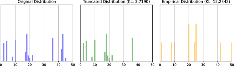
Figure 1: Illustration of the original example distribution, the truncated distribution using the likelihood re-weighting trick and directly approximating the distribution empirically using the same number of random samples.

Specifically, we collect a set (i.e. the collection of unique elements) of decoded data as the truncation basis, and use the original distribution $p$ to assign a normalized weight for each of the unique basis samples. In practice, this can be achieved by either running random sampling multiple times until having collected a sufficient number of unique samples or simply doing a beam search to approximately select the top-$K$ ($K$ is the sample size limit) of $p$ as the truncation basis.

It it trivial to prove that this minimizes the $f_{KL}$ between the truncated distribution and original distribution.

3.4 Compositional Generalization of Different Constraints

In this subsection we concern using NADO to tackle the composition of a collection of constraints $\{C_{i}(\mathbf{x},\mathbf{y})\}$. One straightforward approach is to directly construct a new constraint, denoted as $C$, which is equivalent to taking the logical conjunction (or multiplication of values) of all $C_{i}$. We can then train a single-layered NADO model to handle this composite constraint. This approach is intuitive and avoids the introduction of new assumptions and theoretical analyses. However, its major drawback lies in the implicit assumption of independent and identically distributed (i.i.d.) constraints. In other words, the combination of constraints during the testing phase must exhibit high consistency with the combination of constraints during the training phase. Our primary focus is instead on individually training a NADO layer for each constraint $C_{i}$ in the composition and effectively cascading them to form a structure that ensures a certain level of generalization.

3.4.1 Unitary i.i.d. Constraints and Theoretical Guarantee for Statistically-Independent Constraints

We begin by relaxing the stringent assumption of independent and identically distributed (i.i.d.) constraints, which imposes significant limitations. Instead, we consider a relatively relaxed assumption that we refer to as unitarily i.i.d. Given a combination of constraints, we no longer require the constraint combination during the test phase to be fully i.i.d. with respect to the constraint combination during the training phase. However, we do expect that within each composition, the distribution of each individual constraint maintains a degree of statistical i.i.d. characteristics as observed during the training phase.

We can interpret the impact of each constraint $C_{i}$ on the data distribution as a mapping performed by a single-layered NADO module, which maps the constraint to a corrective term for the original distribution, denoted as $R^{C_{i}}(\mathbf{x},\mathbf{y}_{<t})$. If each constraint within the composition is statistically independent, we can train an individual density ratio function $R$ for each constraint using the base distribution $p$, until we can bound the generalization error of $R$ under the assumption of unitary i.i.d. by $\delta$ on the log-scale. Then, during the test phase, we can directly multiply the corresponding corrective terms induced by the constraints $C_{i}$ with the base distribution $p$. Mathematically, this can be expressed as:

$$q(\mathbf{y}_{<t}|\mathbf{x})=p(\mathbf{y}_{<t}|\mathbf{x})\cdot\prod_{i=1}^{N}R^{C_{i}}(\mathbf{x},\mathbf{y}_{<t})$$

where $q(\mathbf{y}_{<t}|\mathbf{x})$ denotes the distribution of the partial sequence $\mathbf{y}_{<t}$ given input $\mathbf{x}$ during the test phase, and $N$ represents the number of constraints in the composition. It is trivial to bound the error of likelihood from the resulting composed distribution $q$ by $N\cdot\delta$ on the log-scale. This bound is effective for compositionally varied test samples.

Work-around for Weakly-Dependent Constraints

In datasets like CommonGen, although we still assume and aim for compositional generalization, it is important to note that for each set of constraints, the constraints themselves may not be completely statistically independent. Therefore, the aforementioned bound may not hold directly without adjustments. However, considering that in practice, we often use the embedding outputs from the previous NADO layer as inputs for the current layer, we can train each NADO layer to adapt under the following three conditions:

• To accept modified embeddings from the previous NADO layer as input and correctly contextualize them

• To provide an effective embedding for the subsequent NADO layer’s output

• To ensure that the error across the entire embedding distribution can be bounded by $\delta$

By satisfying these conditions, we can still roughly maintain the aforementioned bound. Although this analysis may not be entirely rigorous or comprehensive, given the highly data-specific nature of this problem, extensive assumptions and analyses could be intractable naturally. Nonetheless, this approach provides a significant improvement in terms of generalization guarantees compared to the naive solution of directly multiplying all constraints together.

4 Experiments

We evaluate NADO++ on the supervised Lexically Constrained Generation (LCG) task using the CommonGen dataset(Lin et al., 2020). CommonGen is designed to evaluate the commonsense reasoning ability of neural text generation models, as well as examining their compositional generalization ability. The training set consists of 32,651 unique key concepts, which serve as constraints, and a total of 67,389 annotated description sequences. Additionally, a validation set containing 993 concepts and 4,018 description sequences is provided. To ensure a comprehensive evaluation, the dataset maintains an open leaderboard for benchmarking different approaches on a withheld test set. We closely followed previous paper’s data configurations to ensure consistency with prior work.

We consider the problem as a composition of constraints under two setups: 1) static: lexical + commensensical 2) dynamic the composition of each concept as a independent constraint. For better comparison, we also report the results under a limited setup, where we follow the data setups in vanilla NADO and only concern the algorithmic part of improvements. See Figure 2

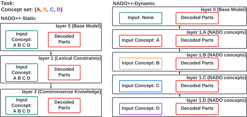
Figure 2: Illustration of the two variants of NADO++ models for CommonGen.

In the following subsections, we would introduce the motivations and technical details for each variant of NADO++.

NADO++-Static: Using an Additional NADO Hierarchy to Remedy Uncommonsensical Generations

The original version of NADO treats CommonGen as a lexically constrained generation problem; however, this perspective is not entirely accurate. Given a set of concepts, for a model that is not finetuned from a sufficiently large checkpoint, ensuring that all lexical conditions are satisfied is insufficient to guarantee that the generated sentences are fully commonsensical. Therefore, we introduce an additional NADO hierarchy to strengthen or, in other words, remedy the flaws of the lexical NADO. To some extent, the commonsensicality of a sentence and the presence of a specific set of lexical constraints are independent of each other. However, considering that we only involve a maximum of two layers in the NADO++ cascaded structure, the aforementioned bound accurately describes the generalization ability between these two layers but does not significantly assist in evaluating the compositional generalization capabilities that CommonGen aims to test.

To provide the $C(\mathbf{x},\mathbf{y})$ for the commonsense layer, we use an semantic role label extractor (the AllenNLP(Gardner et al., 2018) implementation of Shi and Lin (2019)) to parse the given sentence into a series of actions. By using the training set as the positive data and using random replacement of the central verb in the extracted SRLs to construct negative data, we then finetune another t5 model to serve as an approximation of the golden commonsense predictor $C_{\phi}(\mathbf{x},\mathbf{y})$. During training, we use 0/1-quantized version of $C_{\phi}(\mathbf{x},\mathbf{y})$ to serve as commonsense judgements. See Figure3.

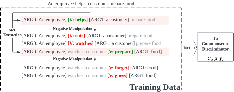
Figure 3: Illustration of the creation of the approximated commonsense $C_{\phi}(\mathbf{x},\mathbf{y})$ model.

For each generated sequence $\mathbf{y}$, the soft-conjunction (i.e. multiplication/AND) of the commonsense prediction on all its extracted SRLs is taken as the approximated $C(\mathbf{x},\mathbf{y})$.

NADO++-Dynamic: A Model that Scales up in Complexity with the Task

Recall that in CommonGen, the difficulty of the task actually varies across instances, largely influenced by the number of constraint words involved. While there is a limit to the number of constraints provided during the test phase, attempting to address a task with varying levels of complexity using a fixed-size model is inherently less practical. This observation forms the basis of NADO++-Dynamic. In this approach, our base model becomes an unsupervised model responsible for learning the overall distribution of commonsensical sequences without any input concepts provided. Each NADO layer aims to address the control of a specific lexical constraint, building upon the weak contextualization introduced by the previous layer’s modified distribution.

Table 1: Results on CommonGen

Model	BLEU	CIDEr	Coverage
T5-Large Finetune	32.81	16.4	92.3%
NADO	34.12	17.4	96.7%
NADO++-Limited	36.71	17.58	97.1%
NADO++-Static	38.42	17.59	96.7%
NADO++-Dynamic (full T5-large NADO layers)	39.91	17.71	98.2%
Naive Bayes	16.4	9.81	45.7%
Naive Bayes w/ Joint Prob. Aug.	29.98	15.9	75.8%

Ablation Study: Has NADO++-Dynamic capture the weakly-dependent nature of constraints?

While we implicitly injected the weak-dependency between layers in a typical NADO structure via passing the hidden output of each hierarchy in the cascading structure, it is unclear whether this practice is sufficient for an effective learning of the mutual correlation of constraints. We add two degraded versions of the model as ablation study towards this matter.

The quantitative results are shown in Table 1.

5 Conclusion

This paper presents an improved training of the NADO algorithm, namely NADO++, and discusses associated theoretical insights. In addition, we discuss the achievable guarantees when using NADO to handle the composition of a set of constraints. The improved training involves a novel parameterization and better sampling/gradient estimation strategy. We demonstrate that NADO++ in general resolves the aforementioned challenges in robustness of NADO, and is able to achieve promising improvements on CommonGen.

References

- Anderson et al. (2017) Peter Anderson, Basura Fernando, Mark Johnson, and Stephen Gould. 2017. Guided open vocabulary image captioning with constrained beam search. In EMNLP, pages 936–945. Association for Computational Linguistics.
- Brown et al. (2020) Tom Brown, Benjamin Mann, Nick Ryder, Melanie Subbiah, Jared D Kaplan, Prafulla Dhariwal, Arvind Neelakantan, Pranav Shyam, Girish Sastry, Amanda Askell, et al. 2020. Language models are few-shot learners. Advances in neural information processing systems, 33:1877–1901.
- Dathathri et al. (2020) Sumanth Dathathri, Andrea Madotto, Janice Lan, Jane Hung, Eric Frank, Piero Molino, Jason Yosinski, and Rosanne Liu. 2020. Plug and play language models: A simple approach to controlled text generation. In ICLR. OpenReview.net.
- Dong et al. (2022) Qingxiu Dong, Lei Li, Damai Dai, Ce Zheng, Zhiyong Wu, Baobao Chang, Xu Sun, Jingjing Xu, and Zhifang Sui. 2022. A survey for in-context learning. arXiv preprint arXiv:2301.00234.
- Gardner et al. (2018) Matt Gardner, Joel Grus, Mark Neumann, Oyvind Tafjord, Pradeep Dasigi, Nelson Liu, Matthew Peters, Michael Schmitz, and Luke Zettlemoyer. 2018. Allennlp: A deep semantic natural language processing platform. arXiv preprint arXiv:1803.07640.
- Keskar et al. (2019) Nitish Shirish Keskar, Bryan McCann, Lav R. Varshney, Caiming Xiong, and Richard Socher. 2019. CTRL: A conditional transformer language model for controllable generation. CoRR, abs/1909.05858.
- Krause et al. (2021) Ben Krause, Akhilesh Deepak Gotmare, Bryan McCann, Nitish Shirish Keskar, Shafiq R. Joty, Richard Socher, and Nazneen Fatema Rajani. 2021. Gedi: Generative discriminator guided sequence generation. In Findings of the Association for Computational Linguistics: EMNLP 2021, Virtual Event / Punta Cana, Dominican Republic, 16-20 November, 2021, pages 4929–4952. Association for Computational Linguistics.
- Lester et al. (2021) Brian Lester, Rami Al-Rfou, and Noah Constant. 2021. The power of scale for parameter-efficient prompt tuning. In EMNLP (1), pages 3045–3059. Association for Computational Linguistics.
- Li and Liang (2021) Xiang Lisa Li and Percy Liang. 2021. Prefix-tuning: Optimizing continuous prompts for generation. In ACL/IJCNLP (1), pages 4582–4597. Association for Computational Linguistics.
- Lin et al. (2020) Bill Yuchen Lin, Wangchunshu Zhou, Ming Shen, Pei Zhou, Chandra Bhagavatula, Yejin Choi, and Xiang Ren. 2020. Commongen: A constrained text generation challenge for generative commonsense reasoning. Findings of EMNLP.
- Lin and Riedl (2021) Zhiyu Lin and Mark O. Riedl. 2021. Plug-and-blend: A framework for plug-and-play controllable story generation with sketches. In AIIDE, pages 58–65. AAAI Press.
- Liu et al. (2021) Alisa Liu, Maarten Sap, Ximing Lu, Swabha Swayamdipta, Chandra Bhagavatula, Noah A. Smith, and Yejin Choi. 2021. Dexperts: Decoding-time controlled text generation with experts and anti-experts. In ACL/IJCNLP (1), pages 6691–6706. Association for Computational Linguistics.
- Lu et al. (2021) Ximing Lu, Peter West, Rowan Zellers, Ronan Le Bras, Chandra Bhagavatula, and Yejin Choi. 2021. Neurologic decoding: (un)supervised neural text generation with predicate logic constraints. In NAACL-HLT, pages 4288–4299. Association for Computational Linguistics.
- Radford et al. (2019) Alec Radford, Jeffrey Wu, Rewon Child, David Luan, Dario Amodei, Ilya Sutskever, et al. 2019. Language models are unsupervised multitask learners. OpenAI blog, 1(8):9.
- Raffel et al. (2020) Colin Raffel, Noam Shazeer, Adam Roberts, Katherine Lee, Sharan Narang, Michael Matena, Yanqi Zhou, Wei Li, and Peter J. Liu. 2020. Exploring the limits of transfer learning with a unified text-to-text transformer. J. Mach. Learn. Res., 21:140:1–140:67.
- Shi and Lin (2019) Peng Shi and Jimmy Lin. 2019. Simple bert models for relation extraction and semantic role labeling. arXiv preprint arXiv:1904.05255.
- Shin et al. (2020) Taylor Shin, Yasaman Razeghi, Robert L. Logan IV, Eric Wallace, and Sameer Singh. 2020. Autoprompt: Eliciting knowledge from language models with automatically generated prompts. In EMNLP (1), pages 4222–4235. Association for Computational Linguistics.
- Yang and Klein (2021) Kevin Yang and Dan Klein. 2021. FUDGE: controlled text generation with future discriminators. In NAACL-HLT, pages 3511–3535. Association for Computational Linguistics.
- Zhang et al. (2022) Hanqing Zhang, Haolin Song, Shaoyu Li, Ming Zhou, and Dawei Song. 2022. A survey of controllable text generation using transformer-based pre-trained language models. CoRR, abs/2201.05337.