m o m o \IfValueTF#2\IfValueTF#4\DeclareAcronym#1short=#2,long=#3,#4 \DeclareAcronym#1short=#2,long=#3 \IfValueTF#4\DeclareAcronym#1short=#1,long=#3,#4 \DeclareAcronym#1short=#1,long=#3 \acro2Dtwo-dimensional \acro3Dthree-dimensional \acro4Dfour-dimensional \acro6Dsix-dimensional \acro1Gfirst generation \acro2Gsecond generation \acro3Gthird generation \acro4Gfourth generation \acro5Gfifth generation \acro5GC5G core network \acro5G-StoRM5G stochastic radio channel for dual mobility \acro6Gsixth generation \acro3GPP3rd generation partnership project \acro3GPP23rd generation partnership project 2 \acroA2Aair-to-air \acroA2Gair-to-ground \acroAAantenna array \acroACadmission control \acroADattack-decay \acroAEantenna element \acroAFamplify and forward \acroABSalmost blank subframe \acroACFautocorrelation function \acroADSLasymmetric digital subscriber line \acroAHWalternate hop-and-wait \acroAIartificial intelligence \acroAMCadaptive modulation and coding \acroAPaccess point \acroAPAadaptive power allocation \acroAPIapplication protocol interface \acroARQautomatic repeat request \acroATaveraged time \acroARMAautoregressive moving average \acroASEaverage squared error \acroASCadaptive satisfaction control \acroATESadaptive throughput-based efficiency-satisfaction trade-off \acroAWGNadditive white gaussian noise \acroBAPbackhaul adaptation protocol \acroBBbranch and bound \acroBCbranch and cut \acroBDblock diagonalization \acroBERbit error rate \acroBFbest fit \acroBLbit loading \acroBLERblock error rate \acroBLPC-1bit loading with power constraint in hop 1 \acroBLPC-2bit loading with power constraint in hop 2 \acroBPCbinary power control \acroBPSKbinary phase-shift keying \acroBRAbalanced random allocation \acroBSbase station \acroBSP\acs*BS placement \acroBSRbuffer status report \acroBoIband of interest \acroC-linkcontrol link \acroCAPcombinatorial allocation problem \acroCAPEXcapital expenditure \acroCBcontextual bandit \acroCBFcoordinated beamforming \acroCBRconstant bit rate \acroCBSclass based scheduling \acroCCcongestion control \acroCCLcommon cell list \acroCDFcumulative distribution function \acroCDLclustered delay line \acroCDMAcode-division multiple access \acroCIRchannel impulse response \acroCHchannel hardening \acroCHOconditional handover \acroC-RANcloud-based radio access network \acroCLclosed loop \acroCLTcentral limit theorem \acroCLPCclosed loop power control \acroCNcore network \acroCNRchannel-to-noise ratio \acroCPcontrol plane \acroCPAcellular protection algorithm \acroCPICHcommon pilot channel \acroCoMPcoordinated multi-point \acroCQIchannel quality indicator \acroCREcell range expansion \acroCRMconstrained rate maximization \acroCRNcognitive radio network \acroC-RNTIcell radio network temporary identifier \acroCRRMcentralized/common radio resource management \acroCRScell-specific reference signal \acroCScoordinated scheduling \acroCSIchannel state information \acroCSI-RSchannel state information reference signal \acroCTSclear to send \acroCUcentralized unit \acroCUEcellular user equipment \acroCWNDcongestion window size \acroD2Ddevice-to-device \acroD2Ndrone-to-network \acroDAAdrone antenna array \acroDAGdirected acyclic graph \acroDBSdrone mounted base station \acroDCdual connectivity \acroDCAdynamic channel allocation \acroDEdifferential evolution \acroDFdecode and forward \acroDFTdiscrete fourier transform \acroDISTdistance \acroDLdownlink \acroDMAdouble moving average \acroDMRSdemodulation reference signal \acroD2DM\acs*D2D mode \acroDMS\acs*D2D mode selection \acroDPdata plane \acroDPCdirty paper coding \acroDRAdynamic resource assignment \acroDSAdynamic spectrum access \acroDSMdelay-based satisfaction maximization \acroDUdistributed unit \acroE2Eend-to-end \acroECCelectronic communications committee \acroEDFearliest deadline first \acroEEenergy efficiency \acroEFLCerror feedback based load control \acroEIefficiency indicator \acroe-ICICenhanced inter-cell interference coordination \acroeMBBenhanced mobile broadband \acroEMelectromagnetic \acroeNBevolved node B \acroEXPexponential \acroEPAequal power allocation \acroEPCevolved packet core \acroEPSevolved packet system \acroE-UTRANevolved universal terrestrial radio access network \acroESexhaustive search \acroFCPfundamental counting principle \acroFCAflow control algorithm \acroFDfull duplex \acroFDDfrequency division duplex \acroFDMfrequency division multiplexing \acroFDMAfrequency division multiple access \acroFERframe erasure rate \acroFIFOfirst in first out \acroFoVfield-of-view \acroFFfast fading \acroFRS[FS]fast-rat scheduling \acroFSfast switching \acroFSBfixed switched beamforming \acroFSTfixed \acs*SNR target \acroFTfourier transform \acroFTPfile transfer protocol \acroFwdforwarding \acroGAgenetic algorithm \acroGAPgeneralized assignment problem \acroGAP-MQgeneralized assignment problem with minimum quantities \acroGATESgeneralized adaptive throughput-based efficiency-satisfaction trade-off \acroGBRguaranteed bit rate \acroGLRgain to leakage ratio \acrogNBgNodeB \acroGOSgenerated orthogonal sequence \acroGPgaussian process \acroGPLGNU general public license \acroGPSglobal positioning system \acroGRPgrouping \acroGSMglobal system for mobile communications \acroGTELwireless telecommunications research group \acroHARQhybrid automatic repeat request \acroHBFhybrid beamforming \acroHCPPhardcore point process \acroHetNetheterogeneous network \acroHDhalf duplex \acroHFhigh-frequency \acroHHhughes-hartogs \acroHardH[HH]hard handover \acroHMSharmonic mode selection \acroHOhandover \acroHOLhead of line \acroHPBWhalf power beamwidth \acroHSDPAhigh speed downlink packet access \acroHSRhigh-speed railway \acroHSPAhigh speed packet access \acroHTTPhypertext transfer protocol \acroIABintegrated access and backhaul \acroICMPinternet control message protocol \acroICIintercell interference \acroICICinter-cell interference coordination \acroIDidentification \acroi.i.d.independent and identically distributed \acroIETFinternet engineering task force \acroIPCindividual power constraint \acroUIDunique identification \acroIIDindependent and identically distributed \acroIIRinfinite impulse response \acroILPinteger linear problem \acroIMTinternational mobile telecommunications \acroINVinverted norm-based grouping \acroIoTinternet of things \acroIPinternet protocol \acroIPv6internet protocol version 6 \acroIRAintegrated resource allocation \acroIRSintelligent reflecting surface \acroISDinter-site distance \acroISIinter symbol interference \acroISMindustrial, scientific and medical \acroITUinternational telecommunication union \acroJOASjoint opportunistic assignment and scheduling \acroJOSjoint opportunistic scheduling \acroJPjoint processing \acroJRAPAPjoint rb assignment and power allocation problem \acroJSjump-stay \acroJSMjoint satisfaction maximization \acroKKTkarush-kuhn-tucker \acroKPIkey performance indicator \acroLAClink admission control \acroLAlink adaptation \acroLBSlocation based service \acroLCload control \acroLOSline of sight \acroLPlinear programming \acroLTElong term evolution \acroLTE-A\acs*LTE-advanced \acroLTE-Advanced\acLTE-A \acroLTE-R\acLTE railway \acroLSPlarge scale parameter \acroMADRDPGmulti-agent deep recurrent deterministic policy gradient \acroMeNBmaster \acs*ENB \acroM2Mmachine-to-machine \acroMACmedium access control \acroMANETmobile ad hoc network \acroMEDSmethod of exact doppler spread \acroMCmodular clock \acroMCPminimal cost power \acroMCSmodulation and coding scheme \acroMDBmeasured delay based \acroMDIminimum \acs*D2D interference \acroMDSMmodified delay-based satisfaction maximization \acroMDUmax-delay-utility \acroMETISmobile and wireless communications enablers for the twenty-twenty information society \acs*5G \acroMFmatched filter \acroMFAPmobile femtocell access point \acroMGmaximum gain \acroMHmulti-hop \acromIABmobile \acIAB \acroMILPmixed integer linear programming \acroMIMOmultiple input multiple output \acroMINLPmixed integer nonlinear programming \acroMIPmixed integer programming \acroMISOmultiple input single output \acroMITmobility interruption time \acroMLmachine learning \acroMLWDFmodified largest weighted delay first \acroMMEmobility management entity \acroMMFmax-min fairness \acrommMAGICmillimetre-wave based mobile radio access network for fifth generation integrated communications \acroMMRPmaximizing the minimal residual power \acroMMRP-LBmaximizing the minimal residual power with lower bound \acroMMSEminimum mean square error \acromMTCmassive machine-type communications \acrommWavemillimeter wave \acroMNmaster node \acroMOSmean opinion score \acroMPFmulticarrier proportional fair \acroMPRPmaximization of the product of the residual powers \acroMRAmaximum rate allocation \acroMRmaximum rate \acroMRCmaximum ratio combining \acroMRNmobile relay node \acroMRTmaximum ratio transmission \acroMRUSmaximum rate with user satisfaction \acroMSmode selection \acroMSEmean squared error \acroMCGmaster cell group \acroMSImulti-stream interference \acroMTmobile termination \acroMTCmachine-type communication \acroIMS\acs*IP multimedia subsystem \acroMTSImultimedia telephony services over \acs*IMS \acroMTSMmodified throughput-based satisfaction maximization \acroMU-MIMOmulti-user multiple input multiple output \acroMUmulti-user \acroMulti-CUTmulti-cell and multi-user and multi-tier \acroNASnon-access stratum \acroNBnode B \acronBSneighbor base station \acroNCLneighbor cell list \acroNCRnetwork-controlled repeater \acroNGnext generation \acroNGCnext generation core network \acroNLPnonlinear programming \acroNLOSnon-line of sight \acroNMSEnormalized mean square error \acroNNneural network \acroNOMAnon-orthogonal multiple access \acroNORMnormalized projection-based grouping \acroNPnon-polynomial time \acroNRnew radio \acroNRTnon-real time \acroNSAnon-stand-alone \acroNSPSnational security and public safety services \acroOBFopportunistic beamforming \acroOFDMAorthogonal frequency division multiple access \acroOFDMorthogonal frequency division multiplexing \acroOFPCopen loop with fractional path loss compensation \acroO2Ioutdoor-to-indoor \acroOLopen loop \acroOLPCopen-loop power control \acroOL-PCopen-loop power control \acroOM[O&M]operational & maintenance \acroOMAorthogonal multiple access \acroOPEXoperational expenditure \acroORAorthogonal resource allocation \acroORBorthogonal random beamforming \acroJO-PFjoint opportunistic proportional fair \acroOSIopen systems interconnection \acroPApower allocation \acroPAIR\acs*D2D pair gain-based grouping \acroPAPRpeak-to-average power ratio \acroP2Ppeer-to-peer \acroPBCHphysical broadcast channel \acroPBSpico base station \acroPCpower control \acroPCIphysical cell \acs*ID \acroPDCPpacket data convergence protocol \acroPDFprobability density function \acroPDUprotocol data unit \acroPERpacket error rate \acroPFproportional fair \acroPGRAprobabilistic graph based resource allocation \acroP-GWpacket data network gateway \acroPHYphysical \acroPLpathloss \acroPLRpacket loss ratio \acroPRABEpower and resource allocation based on quality of experience \acroPRBphysical resource block \acroPROJprojection-based grouping \acroPSDpower spectral density \acroPSDepositive semi-definite \acroProSeproximity services \acroPSpacket scheduling \acroPSOparticle swarm optimization \acroPSSprimary synchronization signal \acroPTASpolynomial-time approximation scheme \acroPTPpoint-to-point \acroPZFprojected zero-forcing \acroQAMquadrature amplitude modulation \acroQHMLWDFqueue-HOL-MLWDF \acroQoEquality of experience \acroQoSquality of service \acroQPSKquadri-phase shift keying \acroQSMqueue-based satisfaction maximization \acroQuaDRiGaquasi deterministic radio channel generator \acroRACHrandom access \acroRAISESreallocation-based assignment for improved spectral efficiency and satisfaction \acroRANradio access network \acroRAresource allocation \acroRAPrb assignment problem \acroRATradio access technology[long-plural-form=radio access technologies] \acroRATErate-based \acroRAUremote antenna unit \acroRBresource block \acroRBGresource block group \acroREFreference grouping \acroRETremote electrical tilt \acroRFradio frequency \acroRLreinforcement learning \acroRLCradio link control \acroRLFradio link failure \acroRMrate maximization \acroRMarural macro \acroRMJ-SNRregion of the minimum joint snr \acroRMECrate maximization under experience constraints \acroRMSEroot-mean-square error \acroRNCradio network controller \acroRNDrandom grouping \acroRNNrecurrent neural network \acroRRAradio resource allocation \acroRRMradio resource management \acroRSCPreceived signal code power \acroRSRPreference signal received power \acroRSRQreference signal received quality \acroRRround robin \acroRISreconfigurable intelligent surfaces \acroRRCradio resource control \acroRSSIreceived signal strength indicator \acroRTreal time \acroRTSrequest to send \acroRUresource unit \acroRUNErudimentary network emulator \acroRVrandom variable \acroRxreceiver \acroRZFregularized zero-forcing \acroSAsubcarrier assignment \acroSACsession admission control \acrosBSserving base station \acroSCsmall cell \acroSCIside control information \acroSCon[SC]single connectivity \acroSCGsecondary cell group \acroSCMspatial channel model \acroSCSsubcarrier spacing \acroSC-FDMAsingle carrier - frequency division multiple access \acroSCRVspatially consistent random variable \acroSDsoft dropping \acroSDAPservice data adaptation protocol \acroS-Dsource-destination \acroSDPCsoft dropping power control \acroSDMspace-division multiplexing \acroSDMAspace-division multiple access \acroSEsquared error \acroSFshadow fading \acroSMDPsemi-markov decision problem \acroSeNBsecondary \acs*ENB \acroSERsymbol error rate \acroSESsimple exponential smoothing \acroS-GWserving gateway \acroSICsuccessive interference cancellation \acroSelfIC[SIC]self interference cancellation \acroSINRsignal to interference-plus-noise ratio \acroSLNRsignal to leakage-plus-noise ratio \acroSNNstrictly non-negative \acroSIsatisfaction indicator \acroSelfI[SI]self interference \acroSIPsession initiation protocol \acroSISOsingle input single output \acroSIMOsingle input multiple output \acroSIRsignal to interference ratio \acroSMsubcarrier matching \acroSMAsimple moving average \acroSMSEspatial-mean-square error \acroSNsecondary node \acroSNRsignal to noise ratio \acroSONself organizing networks \acroSoAstate-of-the-art \acroSoSsum-of-sinusoids \acroSORAsatisfaction oriented resource allocation \acroSORA-NRTsatisfaction-oriented resource allocation for non-real time services \acroSORA-RTsatisfaction-oriented resource allocation for real time services \acroSPsignal processing \acroSPFsingle-carrier proportional fair \acroSRsmart repeater \acroASRadvanced \acSR \acroSRAsequential removal algorithm \acroSRB1signaling radio bearer 1 \acroSRSsounding reference signal \acroSSBsynchronization signal block \acroSSPsmall scale parameter \acroSSSsecondary synchronization signal \acroSTspanning tree \acroSTTDspace time transmit diversity[long-plural-form=space time transmit diversities] \acroSU-MIMOsingle-user multiple input multiple output \acroSUsingle-user \acrotBStarget base station \acroSVDsingular value decomposition \acroTCPtransmission control protocol \acroTDDtime division duplex \acroTDMtime division multiplexing \acroTDMAtime division multiple access \acroTDMedtime division multiplexed \acroTETRAterrestrial trunked radio \acroTPtransmit power \acroTPCtotal power constraint \acroTRtechnical report \acroTTItransmission time interval \acroTTRtime-to-rendezvous \acroTTTtime-to-trigger \acroTSMthroughput-based satisfaction maximization \acroTUtypical urban \acroTVtelevision \acroTVWS\acs*TV white space \acroTxtransmitter \acroUAVunmanned aerial vehicle \acroUABSCuser-assisted bearer split control \acroUDPuser datagram protocol \acroUDNultra-dense networks \acroUEuser equipment \acroUBA\acUE-\acBS association \acroUEPSurgency and efficiency-based packet scheduling \acroUFCfederal university of ceará \acroULAuniform linear array \acroULuplink \acroUMaurban macro \acroUMiurban micro \acroUMTSuniversal mobile telecommunications system \acroUPuser plane \acroUPNuser provided network \acroURAuniform rectangular array \acroURIuniform resource identifier \acroURLLCultra-reliable low-latency communications \acroURMunconstrained rate maximization \acroVBRvariable bit rate \acroVETvariable electrical tilt \acroVMRvehicle-mounted relay \acroVRvirtual resource \acroVoIPvoice over \acs*IP \acroWCDMAwideband code division multiple access \acroWFwater-filling \acroWIDwireless infrastructure drone \acroWi-Fiwireless fidelity \acroWiMAXworldwide interoperability for microwave access \acroWINNERwireless world initiative new radio \acroWLANwireless local area network \acroWMPFweighted multicarrier proportional fair \acroWPwork package \acroWPFweighted proportional fair \acroWSNwireless sensor network \acroWWWworld wide web \acroWFQweighted fair queuing \acroXIXO(single or multiple) input (single or multiple) output \acroXPRcross-polarization power ratio \acroZFzero-forcing \acroZMCSCGzero mean circularly symmetric complex gaussian
System Level Evaluation of Network-Controlled
Repeaters: Performance Improvement of Serving
Cell and Interference Impact on Neighbor Cells
Abstract
Heterogeneous networks have been studied as one of the enablers of network densification. These studies have been intensified to overcome some drawbacks related to propagation in \acpmmWave, such as severe path and penetration losses. One of the promising heterogeneous nodes is \acNCR. It was proposed by the \ac3GPP in Release 18 as a candidate solution to enhance network coverage. In this context, this work performs a system level evaluation to analyze the performance improvement that an \acNCR can cause in its serving cell as well as its interference impact on neighbor cells. Particularly, the results show a considerable improvement on the performance of \acpUE served by the \acNCR, while neighbor \acpUE that receive the \acNCR signal as interference are negatively impacted, but not enough to suffer from outage.
Index Terms:
\acfNCR, wireless backhaul, coverage, \acf5G, \acf6G.I Introduction
Compared to the previous generation of wireless cellular systems, \ac5G networks have explored higher frequencies, e.g., \acpmmWave [1]. Some of the reasons for this interest are the fact that in \acpmmWave there are larger portions of available spectrum and that the required antenna arrays are smaller, which allows the deployment of more antenna elements creating narrow beams with high directional gain [1, 2, 3]. Nonetheless, there are some disadvantages, e.g., suffering from high path and penetration losses [2, 4].
One of the considered solutions to overcome the propagation losses is network densification. However, building from scratch a completely new wired infrastructure is expensive, takes time and, in some places, trenching may not be allowed, like historical areas. Then, nodes with wireless backhaul have emerged as a possible solution for the situations where wired backhaul is not a viable solution [3, 5].
In this context, the present paper focuses on a new node with wireless backhaul called \acNCR [6]. \acNCR was introduced by \ac3GPP in Release 18 [7]. It is an enhanced version of traditional \acRF repeaters. One of the novelties of \acpNCR is the fact that they have beamforming capability that can be controlled by a \acgNB via side control information to improve the communication.
In this paper, we introduce the concept of \acNCR and study the performance of \acNCR-assisted networks. More specifically, this paper performs a system level evaluation to analyze the performance improvement that an \acNCR can cause in its serving cell. Also, we evaluate the effect of the interference that \acpNCR can have on the neighbor cells.
II Network Controlled Repeater
Traditional \acRF repeaters used in previous generations of wireless communications are non-regenerative nodes that amplify and forward a received signal. A direct consequence of this is the increase of interference in the system [8].
The \acNCR concept is an evolution of the \acRF repeaters that use side control information to overcome the negative aspects of traditional repeaters. Side control information that can be used by \acpNCR are [8]:
-
•
ON/OFF information: turn on/off the amplify and forward on a given slot;
-
•
Timing information: dynamic \acDL/\acUL split;
-
•
Spatial \acTx/ \acRx: beamforming capability.
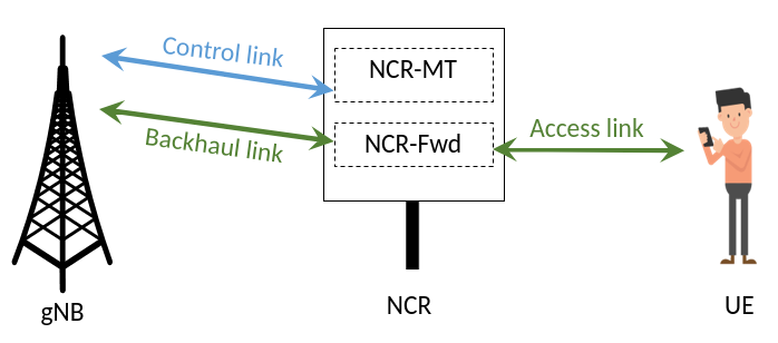
NCR can be split into \acNCR-\acMT and \acNCR-\acFwd, as is shown in Fig. 1. The \acNCR-\acMT is responsible for exchanging side control information with its controlling \acgNB. Its link is called control link, and it is based on \acNR Uu interface. The \acNCR-\acFwd is responsible for executing the \acAF relaying [7].
III System model
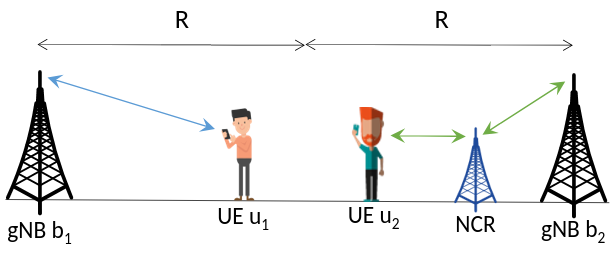
As shown in Fig. 2, consider a scenario with two \acpgNB, i.e., and . The \acISD between them is equal to . Also, consider that there is one \acUE close to each cell edge, i.e., \acpUE and at cells of \acpgNB and , respectively. In the cell of \acgNB , an \acNCR is deployed between and \acUE to enhance the link serving as shown in Fig. 2.
Since we consider that the \acpUE are close to the cell edge, the \acgNB antenna array is deployed such that it steers to the middle point between its respective \acUE and itself. Furthermore, the \acNCR backhaul antenna array is always pointing towards the \acgNB direction, while its access antenna array points towards the \acUE .
Regarding the \acSNR and \acSINR perceived by the \acpUE in the \acDL, their expressions are determined as follows.
Consider a \acPRB as the smallest allocable frequency unit, which consists of a number of adjacent subcarriers in the frequency domain. The system bandwidth is split into \acpPRB. Moreover, consider that \acUE always connects directly to \acgNB , while \acUE connects to \acgNB either directly or through the \acNCR.
The power received by a node from a signal that was transmitted by a node at \acPRB , where the pair can be, for example, , , , , etc., is expressed as
| (1) |
where is the power transmitted by node at \acPRB , is the transmit panel gain of node , is the receive panel gain of node , and is the pathloss between nodes and . Notice that, for the pairs , represents an interfering power, while, for the pairs , represents the useful power.
When \acgNB serves \acUE via \acNCR, the \acNCR transmit power on \acPRB is equal to the \acNCR total receive power, i.e., the sum of the useful power , the noise and the interfering power , amplified by a gain , limited by the \acNCR maximum transmit power per \acPRB . It can be expressed as
| (2) |
We consider that the \acNCR gain can be either fixed or dynamic111Only \acNCR fixed gain has been specified by the \ac3GPP. So, while we try to mimic the model specified by 3GPP Rel-18, the considered setup may have differences with Rel-18 NCR.. When using the dynamic gain, the \acNCR transmit power is always equal to the \acNCR maximum transmit power . For this, the dynamic gain is defined as the ratio between the \acNCR maximum transmit power, i.e., , and \acNCR total receive power, i.e., the sum of the useful power , the noise and the interfering power . We remark that the \acNCR does not need to know the values of , and separately. It just need to know their sum, which is known since it is the total input power that it receives. Thus, the dynamic gain can be expressed as
| (3) |
Regarding the fixed gain, i.e., , it amplifies the total received power with a fixed value, e.g., dB. When the fixed gain implies an \acNCR total transmit power higher than its ceiling , the \acNCR works in a saturated mode. In this mode, it behaves similar to the dynamic gain, where the \acNCR transmit power is equal to the \acNCR maximum transmit power .
Thus, the \acSNR and \acSINR perceived by \acUE at \acPRB are, respectively, given by
| (4) |
and
| (5) |
where is the receiver noise, is the useful power received by at \acPRB and is the interference suffered by at \acPRB .
Regarding , on the one hand, for , the only useful signal received is the one coming from , thus
| (6) |
On the other hand, may receive two components of useful signal, one coming directly from and other being amplified and forwarded by the \acNCR. Thus,
| (7) | |||||
Concerning , with \acNCR, there are two sources of interference for , which are the signal from , with , and this same signal amplified by the \acNCR, thus
| (8) |
Finally, similarly to what has already been presented, regarding , we have
| (9) | |||||
| (10) |
IV Performance Evaluation
IV-A Simulation Assumptions
The simulations were conducted at 28 GHz. The frequency domain was split into \acpPRB consisting of 12 consecutive subcarriers, with subcarrier spacing of 60 kHz. It was adopted the \acRR scheduler for allocating the \acpPRB.
Concerning the time domain, it was split into slots composed of 14 \acOFDM symbols. Each slot had a duration of 0.25 ms. A \acTDD scheme was adopted, where downlink and uplink slots were alternated in time.
Regarding the channel model, the adopted one is based on the \ac3GPP channel model standardized in [9] and its implementation is described in [10]. In this channel model, it is considered a distance-dependent pathloss, a lognormal shadowing component, a small-scale fading, and it is spatially and time consistent. The link types are described in Table I. The \acpgNB and the \acNCR transmissions were performed with a \acDFT codebook based beamforming, where for each transmission a beam management was performed in order to identify the best transmitter beam to be used when serving the \acpUE.
| Link | Scenario | LOS/NLOS |
|---|---|---|
| gNB - UE | Urban Macro | NLOS |
| gNB - NCR | Urban Macro | NLOS |
| NCR - UE | Urban Micro | LOS |
It was used a \acCQI/\acMCS mapping curve standardized in [11] with a target \acBLER of 10 %. An outer loop strategy was considered to avoid the increase of the \acBLER, i.e., when a transmission error occurred, the estimated \acSINR decreased 1 dB, however, when a transmission occurred without error, the estimated SINR had its value added by 0.1 dB. The most relevant simulation parameters are summarized in Tables II and IV-A.
| Parameter | Macro \acgNB | \ac NCR | \ac UE |
|---|---|---|---|
| Height | 25 m | 10 m | 1.5 m |
| Transmit power | 16.8 dBm | 13.8 dBm | 5.8 dBm |
| Antenna array | URA | URA (2 panels) | Single Antenna |
| Antenna element pattern | \ac 3GPP 3D [9] | \ac 3GPP 3D [9] | Omni |
| Max. antenna element gain | 8 dBi | 8 dBi | 0 dBi |
| Parameter | Value |
|---|---|
| Carrier frequency | 28 GHz |
| Subcarrier spacing | 60 kHz |
| Number of subcarriers per \acsRB | |
| Number of \acspRB | |
| Slot duration | 0.25 ms |
| OFDM symbols per slot | |
| Channel generation procedure | As described in [9, Fig.7.6.4-1] |
| Path loss | Eqs. in [9, Table 7.4.1-1] |
| Fast fading | As described in [9, Sec.7.5] and [9, Table 7.5-6] |
| AWGN density power per subcarrier | -174 dBm/Hz |
| Noise figure | 9 dB |
| \acs CBR packet size | bits |
| \Acl ISD | 400 m |
| Distance between \acgNB and \acUE | 150 m |
IV-B Simulation Results
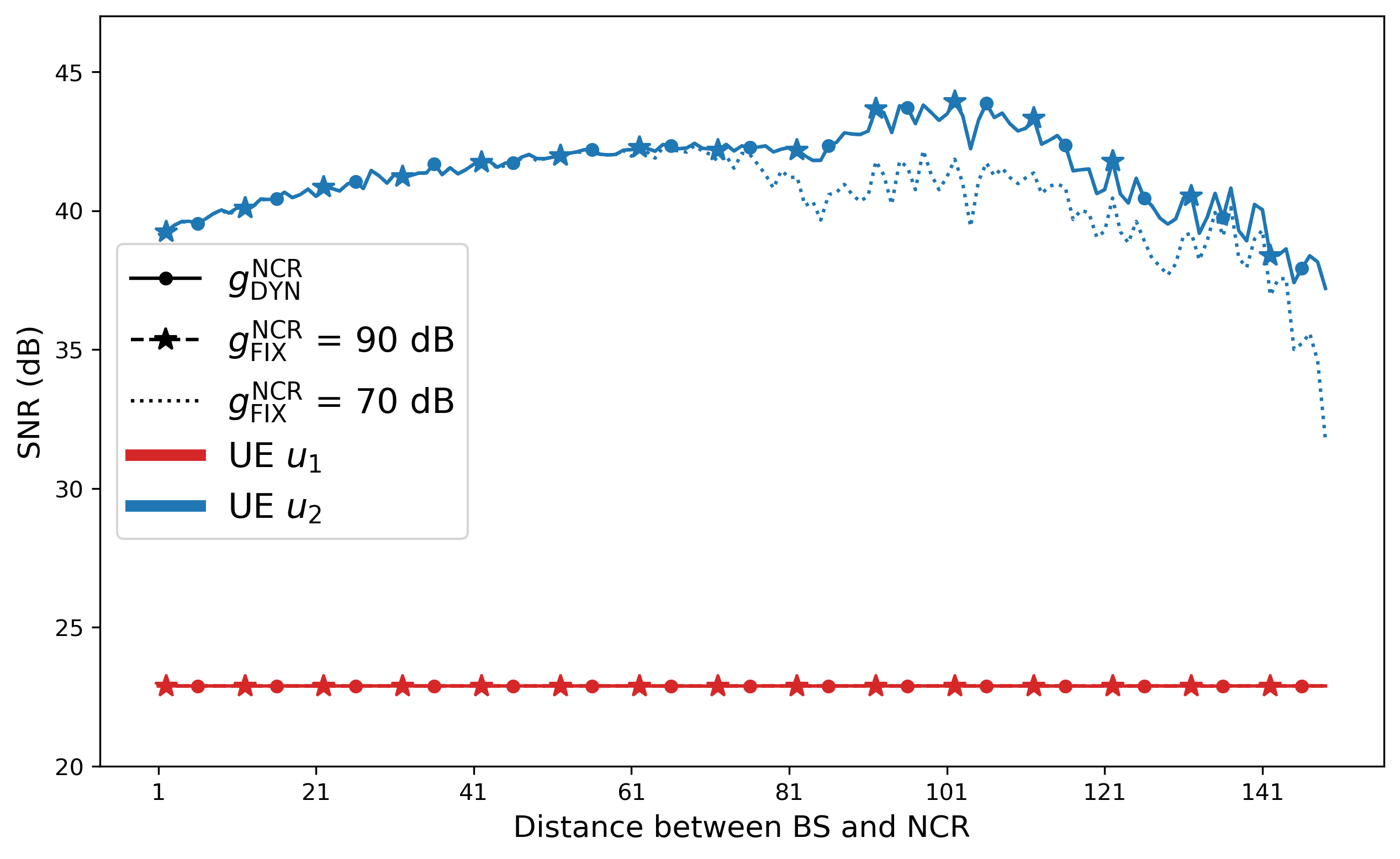
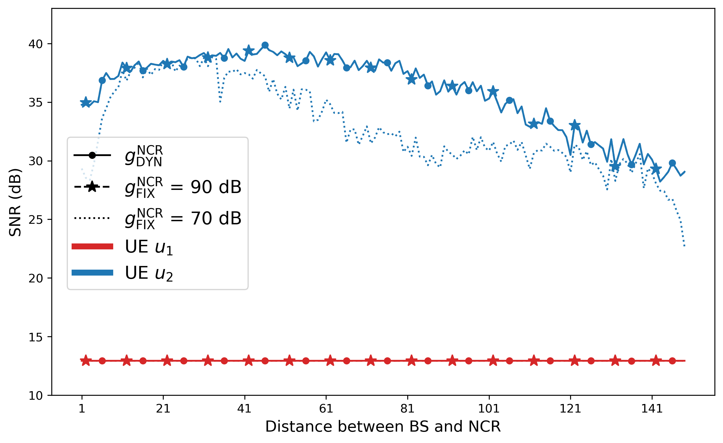
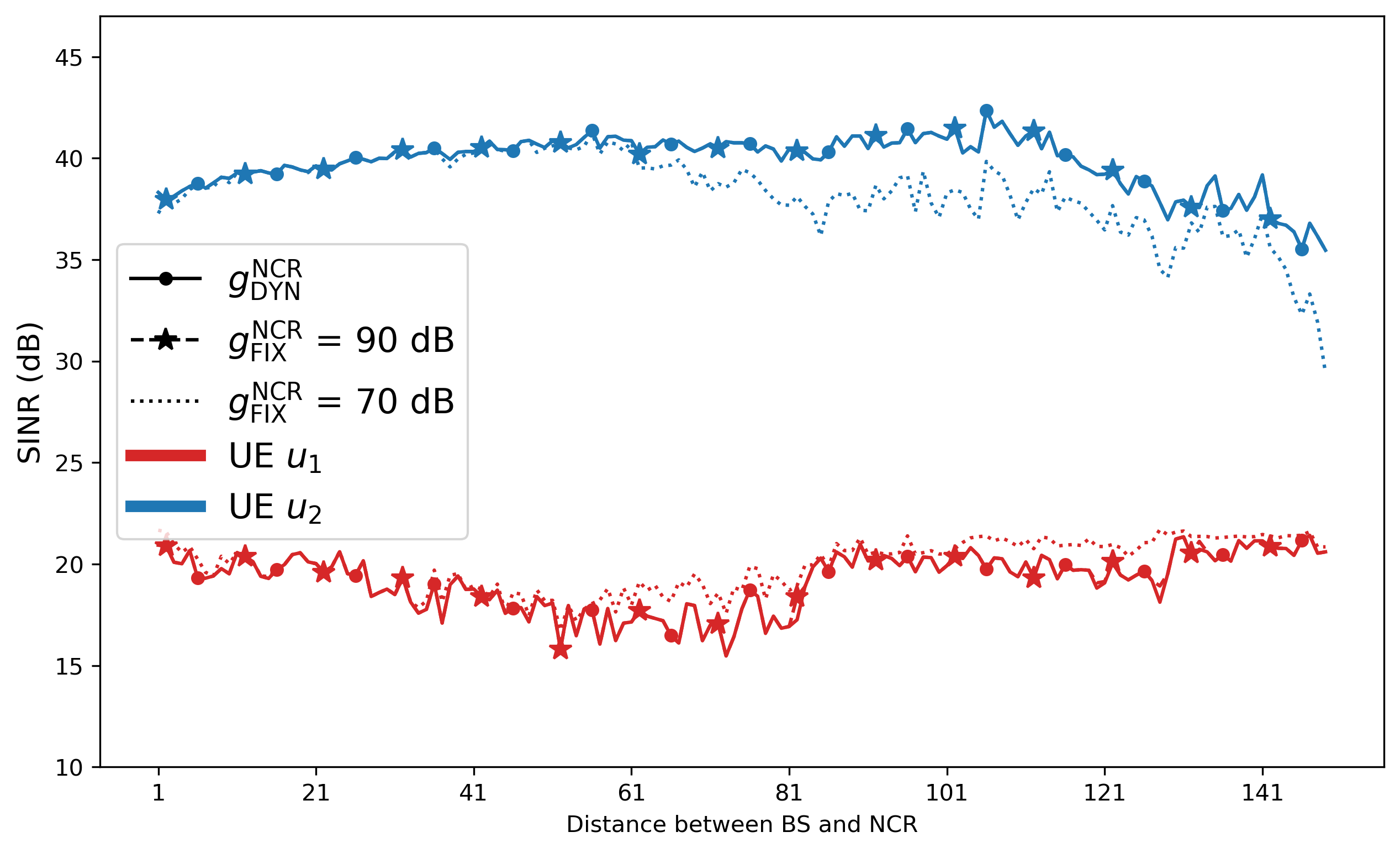
Figures 3 and 4 show the impact of \acNCR position on the \acSNR (quantiles 0.9 and 0.1, respectively) of \acpUE and . Both figures present the results for the two possibilities of the \acNCR gain: dynamic and fixed. For the fixed case, we considered two gain values: 70 dB and 90 dB. Considering the positions of and fixed, the x-axis represents the possible distance between the \acNCR and . As expected, the \acSNR of does not depend of the position of the \acNCR. Also, notice that the \acSNR of , in the beginning, increases and, after a certain distance, starts to decrease. This is due to the product of the two pathlosses in (7), i.e., . Thus, unlike what one could expect, deploying a \acNCR closer to the serving \acUE does not always mean a better connection. In other words, one could expect that the closer a \acUE is to a \acNCR the higher its \acSNR would be due to the shorter distance, and so lower path loss, however as shown in Figs. 3 and 4, this is not true.
Due to the symmetry of the scenario presented in Fig. 2, without the \acNCR, and should present similar values of \acSNR and \acSINR. Thus, by comparing the curves in Fig. 3 and Fig. 4 related to and , we can see that the deployment of an \acNCR considerably improves the \acSNR perceived by . More specifically, the \acSNR perceived by increased in at least 15 dB due to the deployment of the \acNCR. Moreover, notice that the case with fixed \acNCR gain equal to 90 dB presented results similar to the dynamic case, which means that for 90 dB, the \acNCR operated in its saturated mode.
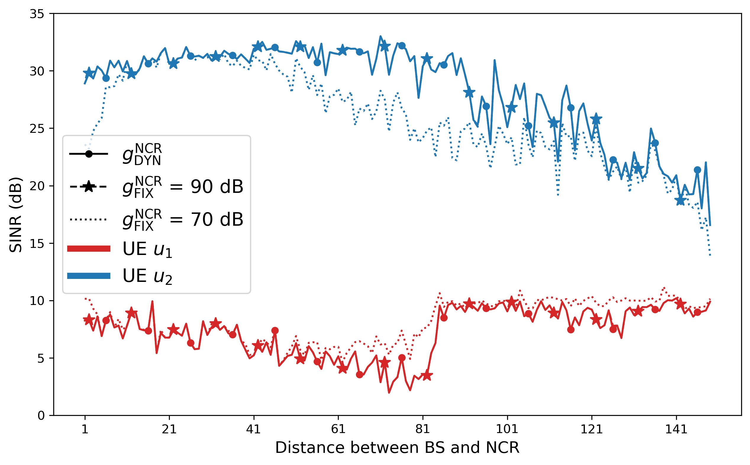
Figures 5 and 6 are similar to Figs. 3 and 4, the main difference is that Figs. 5 and 6 focus on \acSINR instead of \acSNR.
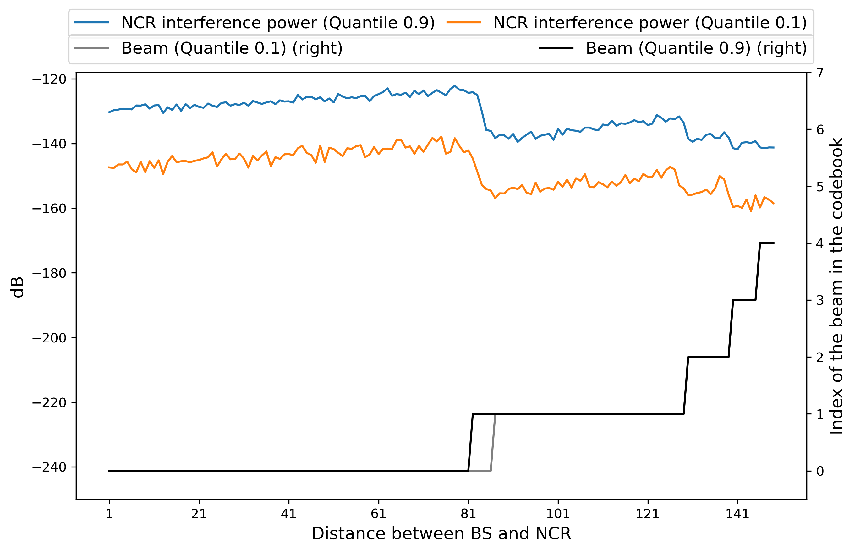
Notice, in Figs. 5 and 6, the trend discontinuity on the \acSINR of when the distance between the \acNCR and is approximately 81 m. This is explained by the change in the interference coming from the \acNCR. More specifically, around that distance the beam used by the \acNCR to serve changes creating a new interference pattern on . Fig. 7 illustrates this behavior.
Fig. 7 presents the impact of the distance between and the \acNCR on the interference suffered by (y-axis of left-hand side) and on the beam index that is used to serve (y-axis of right-hand side). In this figure, we can notice that the interference suffered by has a discontinuity when the distance between and the \acNCR is around 81 m. Around this position, the \acNCR beam serving changes from 0 to 1. Beam 0 points in a direction closer to than Beam 1, that is why when changing from Beam 0 to Beam 1, the interference decreases. This can be seen as a spatial filtering.
Furthermore, notice, in Fig. 7, that within the distance ranges 0 m to 81 m and 81 m to 150 m, the interference suffered by increases when the \acNCR distance between and the \acNCR increases. This is explained by the approximation of the \acNCR to .
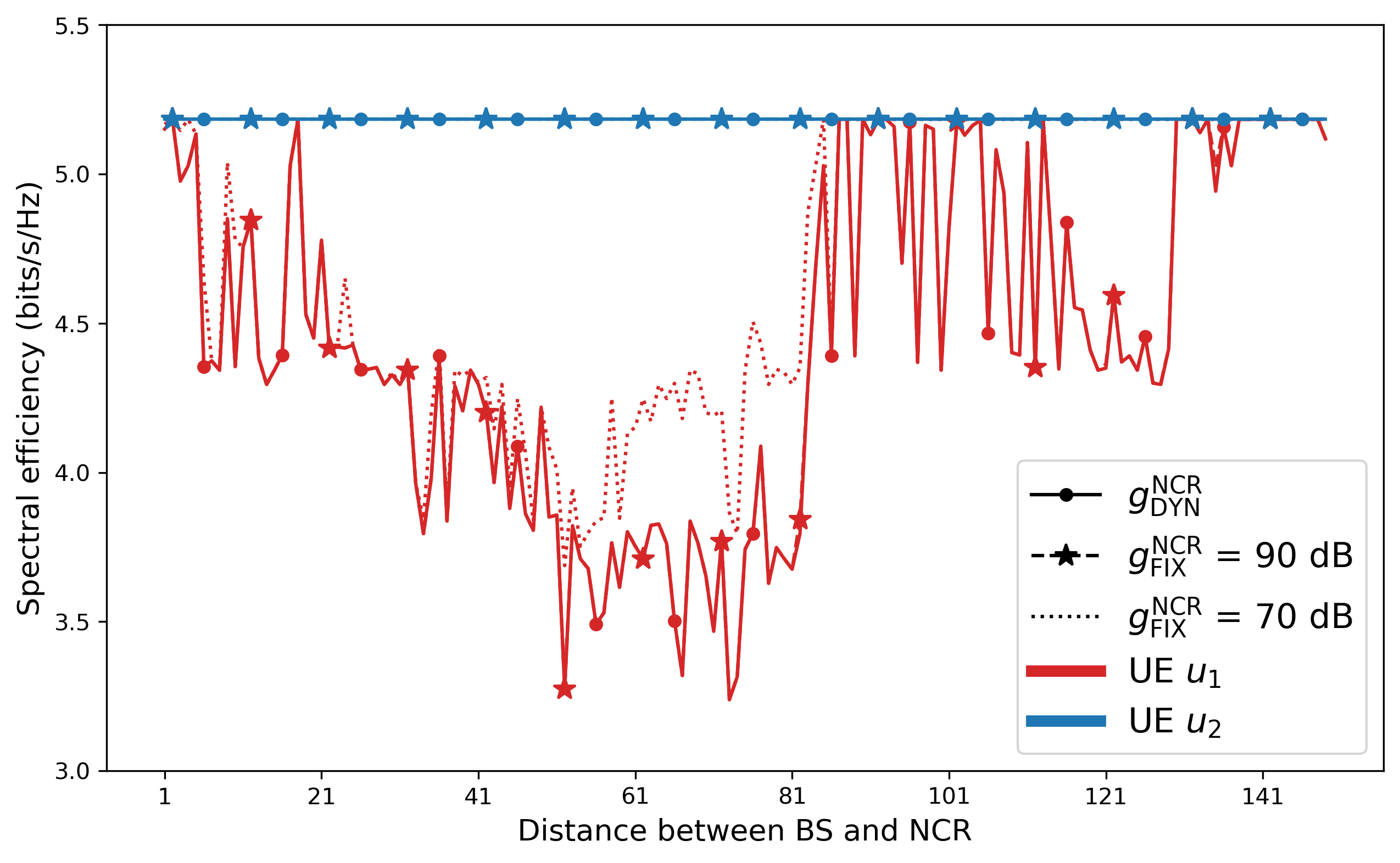
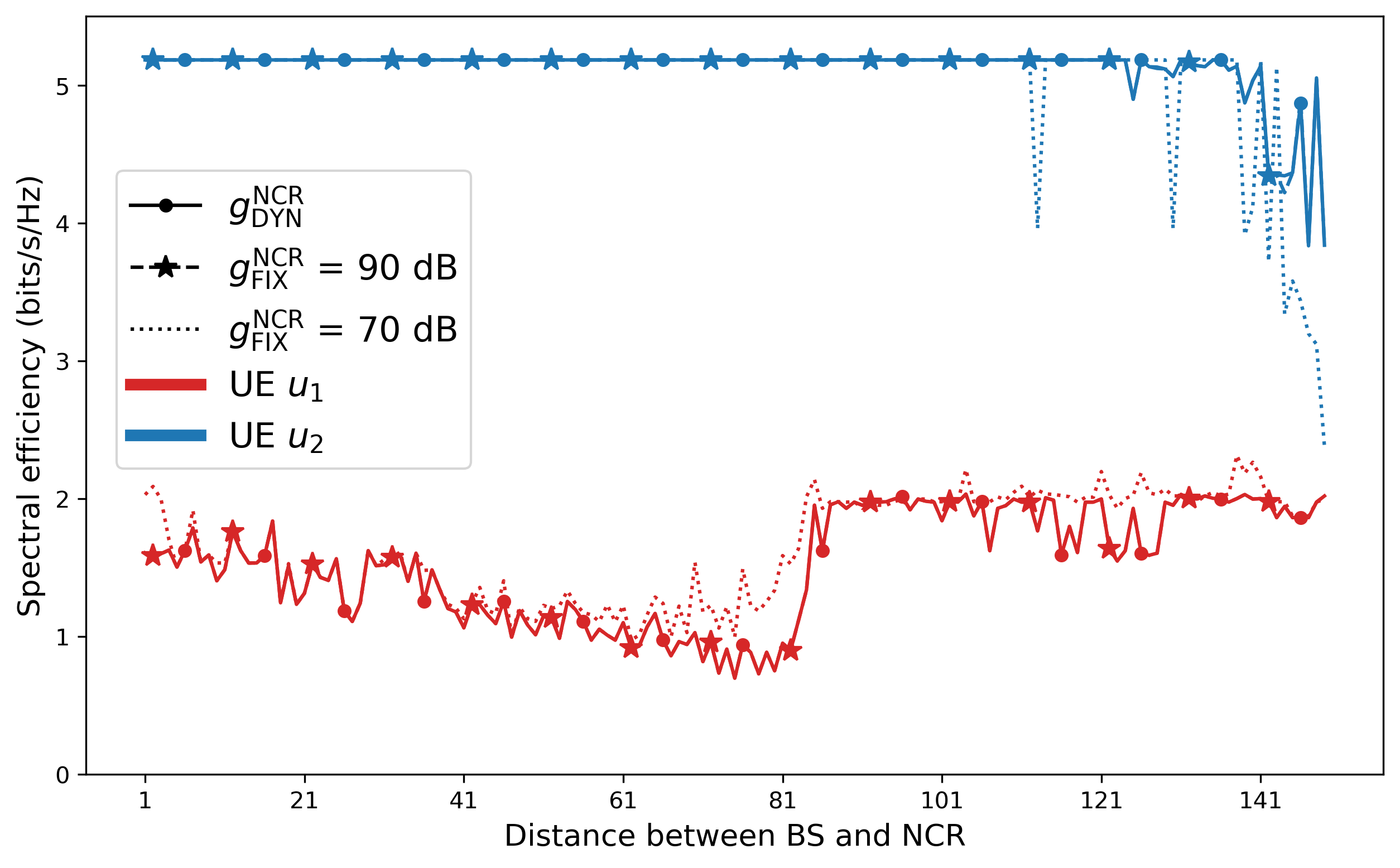
Finally, Figs. 8 and 9 present the impact of the distance between and the \acNCR on the spectral efficiency of the transmissions to and . The maximum spectral efficiency that a transmission could achieve is:
| (11) | |||||
where 5.5547 corresponds to the code rate associated to the \acCQI index 15 in [11]. Remark that achieves the maximum spectral efficiency in the majority of the considered cases, while achieves lower values, but that are still high enough to allow the communication.
V Conclusions
The paper presented a system level evaluation analyzing the performance improvement due to the deployment of a \acNCR on a given cell and its interference impact on neighbor cells. As expected, we have seen that the \acNCR improves the link quality of its serving \acUE. However, unlike what one could expect, deploying a \acNCR closer to its serving \acUE does not necessarily mean a better connection. There is a trade-off given by the product between its distance to its serving \acgNB and its distance to the \acUE that it is serving. We have also seen that the interference caused on neighbor cells can be mitigated by spatial filtering by means of appropriate beam management.
References
- [1] Kai Dong et al. “Advanced Tri-Sectoral Multi-User Millimeter-Wave Smart Repeater”, 2022 arXiv:2210.04859
- [2] Roberto Flamini et al. “Towards a Heterogeneous Smart Electromagnetic Environment for Millimeter-Wave Communications: An Industrial Viewpoint” In IEEE Trans. Antennas Propag. 70.10, 2022, pp. 8898–8910 DOI: 10.1109/TAP.2022.3151978
- [3] Michele Polese et al. “Integrated Access and Backhaul in 5G mmWave Networks: Potential and Challenges” In IEEE Commun. Mag. 58.3, 2020, pp. 62–68 DOI: 10.1109/MCOM.001.1900346
- [4] Reza Aghazadeh Ayoubi et al. “Network-Controlled Repeaters vs. Reconfigurable Intelligent Surfaces for 6G mmW Coverage Extension”, 2022 arXiv:2211.08033
- [5] Charitha Madapatha et al. “On Integrated Access and Backhaul Networks: Current Status and Potentials” In IEEE Open J. Commu. Soc. 1, 2020, pp. 1374–1389 DOI: 10.1109/OJCOMS.2020.3022529
- [6] Hao Guo et al. “A Comparison between Network-Controlled Repeaters and Reconfigurable Intelligent Surfaces”, 2022 arXiv:2211.06974
- [7] 3GPP “Study on NR network-controlled repeaters: Radio Interface Protocol Aspects” v.18.0.0, 2022 URL: http://www.3gpp.org/DynaReport/38867.htm
- [8] “RWS-210019: NR Smart Repeaters”, Qualcomm, 2021
- [9] 3GPP “Study on Channel Model for Frequencies from 0.5 to 100 GHz” v.14.2.0, 2017 URL: http://www.3gpp.org/DynaReport/38901.htm
- [10] Alexandre Matos Pessoa et al. “A Stochastic Channel Model With Dual Mobility for 5G Massive Networks” In IEEE Access 7, 2019, pp. 149971–149987 DOI: 10.1109/ACCESS.2019.2947407
- [11] 3GPP “NR; Physical layer procedures for data” v.15.0.0, 2017 URL: http://www.3gpp.org/ftp/Specs/html-info/38214.htm