Geometric Deep Learning for Structure-Based Drug Design: A Survey

Abstract

Structure-based drug design (SBDD) utilizes the three-dimensional geometry of proteins to identify potential drug candidates. Traditional methods, grounded in physicochemical modeling and informed by domain expertise, are resource-intensive. Recent developments in geometric deep learning, focusing on the integration and processing of 3D geometric data, coupled with the availability of accurate protein 3D structure predictions from tools like AlphaFold, have greatly advanced the field of structure-based drug design. This paper systematically reviews the current state of geometric deep learning in SBDD. We first outline foundational tasks in SBDD, detail prevalent 3D protein representations, and highlight representative predictive and generative models. We then offer in-depth reviews of each key task, including binding site prediction, binding pose generation, de novo molecule generation, linker design, and binding affinity prediction. We provide formal problem definitions and outline each task’s representative methods, datasets, evaluation metrics, and performance benchmarks. Finally, we summarize the current challenges and future opportunities: current challenges in SBDD include oversimplified problem formulations, inadequate out-of-distribution generalization, a lack of reliable evaluation metrics and large-scale benchmarks, and the need for experimental verification and enhanced model understanding; opportunities include leveraging multimodal datasets, integrating domain knowledge, building comprehensive benchmarks, designing criteria based on clinical endpoints, and developing foundation models that broaden the range of design tasks. We also curate https://github.com/zaixizhang/Awesome-SBDD, reflecting ongoing contributions and new datasets in SBDD.

1 Introduction

Structure-based drug design (SBDD) [1, 2, 3] is becoming an essential tool for designing and optimizing drug candidates by effectively leveraging the three-dimensional geometric information of target proteins. Traditionally, the 3D structures of the target protein are obtained with techniques like X-ray crystallography [4], nuclear magnetic resonance (NMR) spectroscopy [5], or cryo-electron microscopy (cryo-EM) [6]. Recently, the progress on high-accurate protein structure prediction such as AlphaFold [7] and ESMFold [8] further boosts the availability of structural data and lays the foundation for its broad applications. SBDD has emerged as an instrumental approach in the development of new kinds of therapies. Several drugs available in the market today owe their genesis to SBDD. For instance, HIV-1 protease inhibitors were identified using this approach [9]. Similarly, raltitrexed, a thymidylate synthase inhibitor [10], and the antibiotic norfloxacin [11] are other exemplars of successful SBDD applications. Nevertheless, conventional SBDD methodologies, which are grounded in physical modeling, the application of hand-engineered scoring functions, and exhaustive search across vast biochemical space, present substantial challenges. In response to these limitations, there has been a burgeoning interest in geometric deep learning [12] to accelerate and refine SBDD.

Geometric deep learning (GDL) [12, 13] refers to neural network architectures designed to capture and encode 3D geometric data. Unlike traditional methods that rely on hand-crafted feature engineering, GDL can autonomously extract salient 3D structural features. Additionally, certain GDL techniques, such as TFN [14], EGNN [15], and GMN [16] that integrate symmetry properties directly into the network design, which serves as an effective inductive bias and potentially leads to enhanced performance. In the realm of 3D Euclidean space, ”symmetry” encompasses transformations like rotations, translations, and reflections. It’s imperative to understand how protein and molecular properties vary under these transformations (Section 2.2). With the rapid development of geometric deep learning, a series of SBDD tasks including binding site prediction [17], binding pose generation [18], de novo ligand generation [19], linker design [20], binding affinity prediction [21], and more [22, 23] have benefited. Geometric deep learning for SBDD has advanced rapidly, drawing more attention from broad communities. Therefore, writing a survey summarizing the recent progress and envisioning the future directions is necessary.

Geometric deep learning for SBDD has two main categories of tasks: predictive [24] and generative tasks [2]. Predictive tasks are concerned with predicting outcomes based on given input protein/molecule data (e.g., binding affinity prediction), demanding high accuracy and reliability due to their applications in drug discovery. On the other hand, generative tasks are centered around the design of new drug molecule data, such as de novo ligand generation. In this paper, we discuss both tasks with an emphasis on exploring the potential and capabilities of the new emerging generative models for SBDD.

1.1 Distinctive Contributions of the Survey

Artificial intelligence is increasingly used to augment all stages of scientific research [25, 26], including designing and developing new therapeutics. We here focus on SBDD, a critical element of therapeutic science underscored by a plethora of surveys detailing its advancements [27, 28, 29, 30, 10, 31, 32]. However, a common thread among these surveys is their vantage point rooted firmly in biochemistry, which may only partially cater to the machine learning research community. Marking a departure from these extant surveys, our review endeavors to bridge this gap. We overview geometric deep-learning methods explicitly tailored for SBDD, elucidated through the lens of machine learning and deep learning paradigms. A standout feature of our review is its meticulous organization, deeply anchored in SBDD task-specific frameworks. More explicitly, we have curated our sections based on distinct SBDD task categories. We have framed each task within a machine learning challenge, ensuring a seamless marriage between domain-specific intricacies and computational methodologies. This entails clearly presenting algorithms, benchmark datasets, evaluation metrics, and model performances for each task. Through this approach, our aim is two-fold: firstly, to enable researchers from the machine learning and deep learning fraternities to gain insights into SBDD tasks without being burdened by intricate domain-specific prerequisites, and secondly, to lay the groundwork that could motivate the development of more sophisticated geometric deep learning algorithms optimally suited for structure-based drug design.

1.2 Organization of the Survey

In this survey, we delve into the interdisciplinary domain bridging geometric deep learning and SBDD. To ensure comprehensive coverage, we curated papers from machine learning conferences and journals, including NeurIPS, ICLR, ICML, KDD, TKDE, and TPAMI. Concurrently, we retrieved publications from natural science journals. Guided by SBDD tasks highlighted in this survey, our search strategy was anchored by key terms, including ”structure-based drug design,” ”protein-ligand docking,” ”protein-ligand affinity prediction,” ”linker design,” and ”protein binding site prediction,” among others, ensuring we amassed a broad spectrum of relevant studies. Given that the majority of FDA-approved drugs fall into the category of small molecules [33], our focus in this survey primarily centers on papers and methodologies that discuss these small molecules. Following our exhaustive search, we meticulously categorized the gathered papers, aligning them with their respective tasks and methodologies. Table I provides a detailed breakdown.

In Section 2.1, we introduce 3D representations of proteins, the SBDD tasks reviewed in this paper, and popular predictive and generative models. The following sections are organized based on the logical order of SBDD tasks as shown in Figure 1: as for the target protein structure, we first need to identify the binding site; then we can conduct binding pose generation, de novo molecule generation, and linker design; with the protein-ligand complex structure, we can use binding affinity prediction and other filtering criteria to filter drug candidates. Admittedly, the order and the category of SBDD tasks are not fixed since SBDD is an iterative process that proceeds through multiple cycles, leading optimized drug candidates to clinical trials [34]. Some methods may also be capable of accomplishing multiple tasks. For example, EquiBind [35] can predict the binding pose of ligands without prior knowledge of the binding site, i.e., blinding docking, to ease readers’ understanding. Finally, Section 4 identifies the open challenges and opportunities, paving the way for the future of designing geometric deep learning methods for structure-based drug design.

2 Preliminaries

Figure 1 provides an overview of the SBDD tasks encompassing binding site prediction, binding pose generation, de novo molecule generation, linker design, and binding affinity prediction. Binding site and affinity prediction are typically formulated as predictive tasks, whereas binding pose generation, de novo molecule generation, and linker design are addressed as generative tasks.

2.1 Protein and Ligand Representations

Protein and ligand molecule representations depend on the SBDD tasks and specific geometric deep learning methods. In SBDD, proteins are usually characterized by 3D representations that capture critical 3D structural information in the form of grids, surfaces, and spatial graphs (Figure 2):

• 3D grids are Euclidean data structures comprised of uniformly spaced 3D elements, termed voxels. These grids have distinct geometric properties: each voxel has a consistent neighborhood structure, making it indistinguishable from other voxels in terms of structure, and the vertices maintain a fixed order determined by their spatial dimensions. Owing to the Euclidean nature of the 3D grid input, 3D CNNs are conventionally employed to encode such data and to handle subsequent tasks.

• The 3D surface of a protein is the exterior layer of the protein’s atoms and is pivotal in protein-ligand interactions. Each point on this protein surface can be distinguished by its associated chemical (e.g., hydrophobic, electrostatic) and geometric (e.g., local shape, curvature) attributes. Protein surfaces can be represented as meshes, polygons that demarcate the surface’s contours, or point clouds, sets of nodes that specify the surface’s position at a particular resolution level.

• 3D graphs are prevalently utilized to describe protein structural data, wherein atoms serve as nodes and covalent bonds as edges. Edges can also be formed by linking the k-nearest neighbors. Geometric GNNs [15, 36] are adept at processing protein 3D graphs.

As for the ligand molecules, their representations vary from 1D strings, e.g., simplified molecular-input line-entry system (SMILES) [37] to 2D and 3D graphs [38] where nodes represent atoms and edges represent bonds (Figure 3).

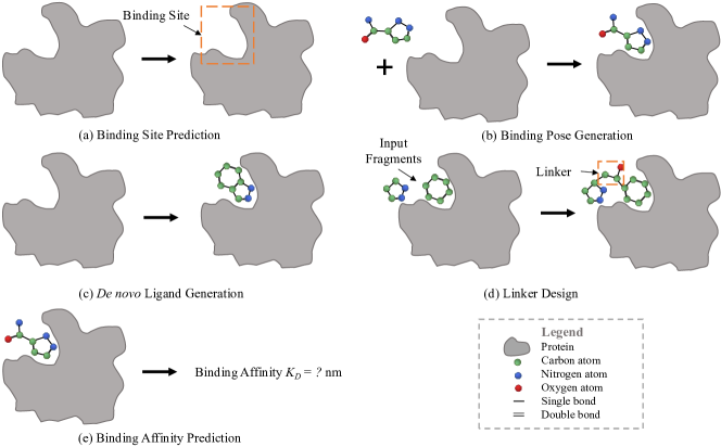
Figure 1: Structure-based drug design tasks discussed in this survey: (a) binding site prediction identifies areas of the protein structure that can act as binding sites for ligands (Section 3.1); (b) binding pose generation or protein-ligand docking focus on predicting the binding conformations of the protein-ligand complex (Section 3.2); (c) de novo ligand generation designs binding ligands from scratch with the structural information of the target protein (Section 3.3); (d) linker design combines disconnected molecular fragments into a combined ligand molecule conditioned on the target protein (Section 3.4); (e) binding affinity prediction predicts the affinity between a protein and a ligand given their binding structure (Section 3.5).

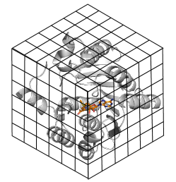
(a) 3D grid

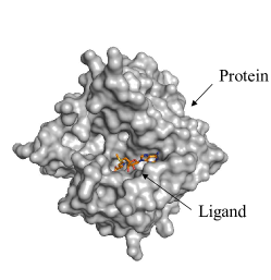
(b) 3D surface

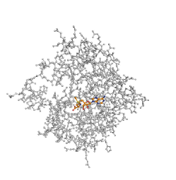
(c) 3D graph

Figure 2: 3D representations of proteins used for geometric deep learning: (a) 3D grid, (b) 3D surface, and (c) 3D graph, illustrated for PDB ID 2avd.

2.2 Symmetries

Incorporating the symmetry priors into neural network architectures as inductive bias is an effective strategy to build generalizable models [39, 12]. The main symmetry groups in protein-ligand systems include the Euclidean group E(3), the particular Euclidean group SE(3), and the permutation group [12]. Both E(3) and SE(3) include rotation and translation transformations in the 3D Euclidean space. E(3) further covers the reflection operation. These transformations are essential for geometric deep learning because the output should obey the underlying physics rules that predicted properties of proteins/ligands should not change under the transformation of coordinate systems and atom orders. SE(3) is applicable when a neural network aims to differentiate chiral systems [40], which are systems that are not superimposable on their mirror images, much like left and right human hands. In chemistry and biology, chiral molecules can exhibit unique properties, e.g., a drug might be therapeutic, while its mirror image might be harmful or inactive. Formally, let $\mathcal{T}$ denote the transformation, $f$ be the neural network, and ${\bm{x}}$ be the input data. The output of the neural network $f({\bm{x}})$ can transform equivariantly or invariantly with respect to $\mathcal{T}$ if satisfy the following constraints:

• Equivariance: $f({\bm{x}})$ is equivariant to a transformation $\mathcal{T}$ if the transformation of input ${\bm{x}}$ commutes with the transformation of $f({\bm{x}})$ via a transformation $\mathcal{T}^{\prime}$ of the same symmetry group, i.e, $f(\mathcal{T}({\bm{x}}))=\mathcal{T}^{\prime}f({\bm{x}})$. Such symmetry is important as the predicted vector outputs (e.g., forces, coordinates) should not depend on the choice of coordinate systems.

• Invariance: Invariance is a special case of equivariance where $f({\bm{x}})$ is invariant to $\mathcal{T}$ if $\mathcal{T}^{\prime}$ is the identity transformation: $f(\mathcal{T}({\bm{x}}))=\mathcal{T}^{\prime}f({\bm{x}})=f({\bm{x}})$. Such symmetry prior is important as the predicted scalar properties of a certain molecule/protein (e.g., energies) should be the same under the transformation of coordinate systems.

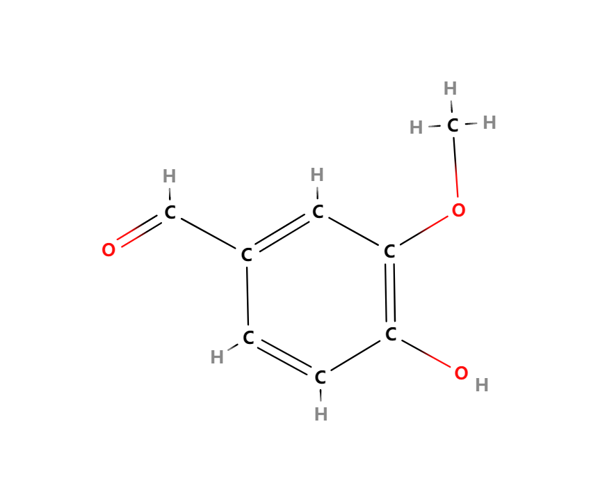
(a) 2D molecular graph

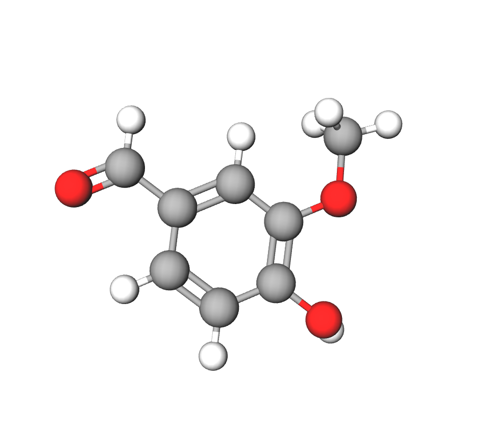
(b) 3D molecular graph

Figure 3: Representing molecules as (a) 2D graphs and (b) 3D graphs.

2.3 Predictive Methods

Next we summarize the main predictive methods for predictive tasks, i.e., binding site and affinity predictions. These methods are also widely used as the structure encoding backbones for generative models.

2.3.1 Convolutional Neural Networks (CNNs)

CNNs are widely used for image processing where the input elements, i.e., pixels, are arranged spatially. CNNs rely on the shared-weight architecture of convolution kernels or filters that slide along input features and provide translation-equivariant outputs. Convolution kernels and filters can vary with data structure. For example, for the 3D surface data, MaSIF [17] defines geodesic convolutional layers with the geodesic polar coordinates. For the 3D grid data, 3D CNNs are widely used [41, 42].

2.3.2 Graph Neural Networks (GNNs)

GNNs are widely used to model relational data. Most GNNs follow a message-passing paradigm. Let the $h_{i}$ be the node feature of the $i$-th node in the graph and $e_{ij}$ be the edge feature for the optional edge connecting node $i$ and $j$. GNNs iteratively conduct message computation and neighborhood aggregation operations for each node (or edge). Generally, we have:

$$m_{ij} =\psi_{m}(h_{i},h_{j},e_{ij}),$$ (1)

$$h_{i}^{\prime} =\psi_{h}(\{m_{ij}\}_{j\in\mathcal{N}(i)},h_{i}),$$ (2)

where $\mathcal{N}(i)$ denote the set of neighbors of node $i$, $h_{i}^{\prime}$ is the updated node feature, and $\psi_{m},\psi_{h}$ are learnable functions.

For the 3D structural data, each node in the 3D graph has scalar features and contains 3D coordinates. Equivariant graph neural networks are proposed to incorporate geometric symmetry into model building [43]. Let $\bm{v}_{i}\in\mathbb{R}^{3}$ denote the 3D coordinate, we have:

$$m_{ij} =\psi_{m}(\bm{v}_{i},\bm{v}_{j},h_{i},h_{j},e_{ij}),$$ (3)

$$\bm{m}_{ij} =\psi_{\bm{m}}(\bm{v}_{i},\bm{v}_{j},h_{i},h_{j},e_{ij}),$$ (4)

$$h_{i}^{\prime} =\psi_{h}(\{m_{ij}\}_{j\in\mathcal{N}(i)},h_{i}),$$ (5)

$$\bm{v}_{i}^{\prime} =\psi_{\bm{v}}(\{\bm{m}_{ij}\}_{j\in\mathcal{N}(i)},\bm{v}_{i}),$$ (6)

where $m_{ij}$ and $\bm{m}_{ij}$ are scalar and vector messages. $\psi_{m}$ and $\psi_{h}$ are geometrically invariant functions while $\psi_{\bm{m}}$ and $\psi_{\bm{v}}$ are geometrically equivariant functions. Compared with traditional 3D CNNs, geometrically equivariant GNNs do not require the voxelization of input data while still maintaining the desirable equivariance. Some representative equivariant GNNs are SchNet [44], EGNN [15], GVP [45], DimeNet [46, 47], GMN [16], SphereNet [48], and ComENet [49].

2.3.3 Graph Transformers

Transformers were originally developed for sequential data [50]. Transformer architectures were recently adapted to 2D and 3D graph data and achieved superior performance [51, 52, 53, 54, 55] than GNNs on node and graph classification tasks. A transformer is composed of stacked transformer blocks, where each block consists of two layers: a self-attention layer followed by a feed-forward layer with normalizations (e.g., LayerNorm [56]) and skip connections for both layers. For an input feature matrix $\textit{{H}}^{(l)}$, the $(l+1)$-th self-attention block works as follows:

$$\textit{{A}}^{(l)} ={\rm softmax}\left(\frac{\textit{{H}}^{(l)}\textit{{W}}^{(l)}_{Q}(\textit{{H}}^{(l)}\textit{{W}}^{(l)}_{K})^{\top}}{\sqrt{d}}\right);$$ (7)

$$\textit{{H}}^{(l+1)} =\textit{{H}}^{(l)}+\sum_{i=1}^{B}\textit{{A}}^{(l)}\textit{{H}}^{(l)}\textit{{W}}^{(l)}_{V}\textit{{W}}^{(l)}_{O},$$ (8)

where A is the attention matrix, $B$ is the total number of attention heads, $d$ is the dimension size, $\textit{{W}}^{(l)}_{Q}$, $\textit{{W}}^{(l)}_{K}$, and $\textit{{W}}^{(l)}_{V}$ are learnable transformation matrices at layer $l$.

To generalize transformers to graphs, positional encodings are indispensable for encoding topological and geometric information [51, 55]. Popular positional encodings are based on shortest paths [51], PageRank [57], and eigenvectors [58]. Positional encodings are necessary for graph transformers to consider graph connectivity–without positional encodings the models would ignore the strong inductive bias of edges and would attend to any pair of nodes. Representative graph transformers include Graphormer [51], Transformer-M [55], and Equiformer [54]. For example, Transformer-M [55] develops two separated channels to encode both 2D and 3D structural information of molecules. The 2D channel uses encodings based on atom degrees, shortest path distance, and 2D graph structure. In the 3D channel, Gaussian basis kernel functions [59] are used to encode 3D spatial distances between atoms.

2.4 Generative Methods

Next section summarizes generative methods for SBDD tasks, including autoregressive models, flow models, variational autoencoders, and diffusion models.

2.4.1 Autoregressive Models (ARs)

A data point ${\bm{x}}$ can be factorized into a set of components $\{x_{0},x_{1},\dots,x_{d-1}\}$, where $d$ is the number of components. These components can be pixels in images and nodes and edges in graphs. The components may have complicated underlying dependencies, making the direct generation of ${\bm{x}}$ challenging. With predefined or learned orders, the autoregressive models factorize the joint distribution of ${\bm{x}}$ into the product of $d$ likelihoods as follows:

$$\small{p({\bm{x}})=\prod_{i=1}^{d}p(x_{i}|x_{1},x_{2},...,x_{i-1}).}$$ (9)

Autoregressive models sequentially generate ${\bm{x}}$: In each step of a generative process, the next subcomponent is predicted based on the previously generated subcomponents.

2.4.2 Flow Models

A flow model aims to learn a parameterized invertible function between a data point x and the latent variable ${\bm{z}}$: $f:{\bm{z}}\in\mathbb{R}^{d}\xrightarrow{}{\bm{x}}\in\mathbb{R}^{d}$. The latent distribution $p({\bm{z}})$ is a predefined probability distribution, e.g., a Gaussian distribution. The data distribution $p({\bm{x}})$ is unknown. But given a data point ${\bm{x}}$, its likelihood can be computed with the change-of-variable theorem:

$$\small{p({\bm{x}})=p({\bm{z}})\Big{|}\text{det}\Big{(}\frac{df^{-1}({\bm{x}})}{d{\bm{x}}}\Big{)}\Big{|},}$$ (10)

where $\text{det}(\cdot)$ is the matrix determinant and $\frac{df^{-1}({\bm{x}})}{d{\bm{x}}}$ is the Jacobian matrix.

In the sampling process, a latent variable ${\bm{z}}$ is first sampled from a predefined latent distribution $p({\bm{z}})$. Then the corresponding data point ${\bm{x}}$ is obtained by performing a feedforward transformation ${\bm{x}}=f({\bm{z}})$. Therefore, $f$ must be differentiable, and the computation of ${\rm det}J$ should be tractable for training and sampling efficiency. A common choice is the affine coupling layers [60, 61] where the computation of ${\rm det}J$ is very efficient because $J$ is an upper triangular matrix.

2.4.3 Variational Autoencoders (VAEs)

Variational autoencoders (VAEs) [62] maximize the evidence lower bound (ELBO) of $p({\bm{x}})$. VAEs introduce the latent variable ${\bm{z}}$ to express the likelihood of ${\bm{x}}$ as:

$$\small\log p({\bm{x}}) =\log\int_{\bm{z}}p({\bm{z}})p({\bm{x}}|{\bm{z}})d{\bm{z}}$$ (11)

$$\geq\mathbb{E}_{q({\bm{z}}|{\bm{x}})}\big{[}\log p({\bm{x}}|{\bm{z}})\big{]}-D_{KL}(q({\bm{z}}|{\bm{x}})||p({\bm{z}}))$$ (12)

$$\triangleq\text{ELBO}.$$ (13)

Here, $p({\bm{z}})$ represents the prior distribution of ${\bm{x}}$. For tractable calculation, parameterized encoder $q({\bm{z}}|{\bm{x}})$ is usually used to approximate $p({\bm{z}}|{\bm{x}})$, also known as the variational inference technique. The first term of ELBO is reconstruction loss, which quantifies the information loss of reconstructing ${\bm{x}}$ from latent representations. The standard Gaussian prior $p({\bm{z}})\sim\mathcal{N}(0,\textit{{I}})$ typically leads to mean-squared error (MSE) loss for the first term. The second term in ELBO is the KL-divergence term, ensuring that our learned distribution $q({\bm{z}}|{\bm{x}})$ is similar to the true prior distribution.

2.4.4 Diffusion Probabilistic Models

Diffusion models [63, 64] are generative models inspired by non-equilibrium thermodynamics. A diffusion model defines a Markovian chain of random diffusion process where each step adds noise to the data, and then it learns the reverse of this process via neural networks to reconstruct data points from noise distributions, e.g., isotropic Gaussian.

Let ${\bm{x}}_{0}\sim p({\bm{x}})$ denote the input data point and ${\bm{x}}_{t}$ for $t=1,\dots,T$ indicate a series of noised representations with the same dimension as ${\bm{x}}_{0}$. The forward diffusion process can be expressed as:

$$q({\bm{x}}_{t}|{\bm{x}}_{t-1}) =\mathcal{N}({\bm{x}}_{t};\sqrt{1-\beta_{t}}{\bm{x}}_{t-1},\beta_{t}\textit{{I}}),$$ (14)

where $\beta_{t}\in(0,1)$ controls the strength of Gaussian noise added in each step. A desirable property of the diffusion process is that a closed form of the intermediate state can be obtained. Let $\alpha_{t}=1-\beta_{t}$, and $\bar{\alpha}_{t}=\prod_{i=1}^{t}\alpha_{i}$, we have:

$$\small{q({\bm{x}}_{t}|{\bm{x}}_{0})=\mathcal{N}({\bm{x}}_{t};\sqrt{\bar{\alpha}_{t}}{\bm{x}}_{0},(1-\bar{\alpha}_{t})\textit{{I}}).}$$ (15)

Another desirable feature of the reverse diffusion process, i.e., the denoising process, is that it can be computed in a closed form when conditioned on ${\bm{x}}_{0}$ using Bayes theorem:

$$p_{\theta}({\bm{x}}_{t-1}|{\bm{x}}_{t}) =\mathcal{N}({\bm{x}}_{t-1};\bm{\mu}_{t}({\bm{x}}_{0},{\bm{x}}_{t}),\widetilde{\beta}_{t}\textit{{I}}),$$ (16)

where the parameters can be obtained analytically:

$$\bm{\mu}_{t}({\bm{x}}_{0},{\bm{x}}_{t}) =\frac{\sqrt{\bar{\alpha}_{t-1}}\beta_{t}}{1-\bar{\alpha}_{t}}{\bm{x}}_{0}+\frac{\sqrt{\alpha_{t}}(1-\bar{\alpha}_{t-1})}{1-\bar{\alpha}_{t}}{\bm{x}}_{t},$$ (17)

$$\widetilde{\beta}_{t} =\frac{1-\bar{\alpha}_{t-1}}{1-\bar{\alpha}_{t}}\beta_{t}.$$

Similar to variational autoencoders, the objective of diffusion models is to maximize the variational lower bound of log-likelihood of $p({\bm{x}})$ as:

$$-\log p({\bm{x}})\leq\underbrace{KL[q({\bm{x}}_{T}|{\bm{x}}_{0})||p_{\theta}({\bm{x}}_{T})]}_{\rm prior\ loss\ \mathcal{L}_{T}}$$

$$~{}~{}~{}+\sum_{t=2}^{T}\underbrace{KL[q({\bm{x}}_{t-1}|{\bm{x}}_{t},{\bm{x}}_{0})||p_{\theta}({\bm{x}}_{t-1}|{\bm{x}}_{t})]}_{\rm diffusion\ loss\ \mathcal{L}_{t-1}}-\underbrace{\mathbb{E}_{q}[\log p_{\theta}({\bm{x}}_{0}|{\bm{x}}_{1})]}_{\rm reconstruction\ loss\ \mathcal{L}_{0}}.$$

Here, $\mathcal{L}_{T}$ is a constant and $\mathcal{L}_{0}$ can be estimated using an auxiliary model [64, 65]. For $\{\mathcal{L}_{t-1}\}_{t=2}^{T}$, diffusion models adopt a neural network $\epsilon_{\theta}$ to predict the noise. More specifically, we can reparameterize Equation 15 as ${\bm{x}}_{t}=\sqrt{\bar{\alpha}_{t}}{\bm{x}}_{0}+\sqrt{(1-\bar{\alpha}_{t})}\epsilon_{t},\epsilon_{t}\sim\mathcal{N}(0,\textit{{I}})$. The following training objective is widely adopted:

$$\small{\mathcal{L}=\mathbb{E}_{t}\Big{[}\|\epsilon_{t}-\epsilon_{\theta}({\bm{x}}_{t},t)\|^{2}\Big{]}.}$$

2.5 Other Methods

Apart from the generative methods previously discussed, several alternative techniques such as Reinforcement Learning (RL) [66], Genetic Algorithm (GA) [67], and Monte Carlo Tree Search (MCTS) [21, 52] are utilized to probe the chemical space for properties of interest. Additionally, drawing inspiration from molecular dynamics and fragment-based drug design, innovative methods grounded on virtual dynamics (VD) [68] and fragment-based molecule generation (Fragment) [69] have been introduced. For instance, in generating 3D molecules suited to a target protein, VD-Gen [68] initializes numerous virtual particles within the pocket. These particles are then iteratively adjusted to mirror the spatial arrangement of molecular atoms. A 3D molecule is subsequently derived from the stabilized virtual particles. In contrast, in fragment-based molecule generation, a motif vocabulary is initially established by isolating prevalent molecular fragments (referred to as motifs) from the dataset. During the generative phase, molecules are generated by autoregressively appending new fragments, ensuring the resulting local structures maintain realism.

TABLE I: Summary of structure-based drug design models with geometric deep learning reviewed in this paper.

Task	Model	Input	Output	Method
Binding site prediction	MaSIF [17]	Protein Surface	Binding Site Probability	CNN
	dMaSIF [70]	Protein Surface	Binding Site Probability	CNN
	PeSTo [71]	Protein 3D-Graph	Binding Site Probability	Transformer
	ScanNet [72]	Protein 3D-Graph	Binding Site Probability	GNN
	PocketMiner [73]	Protein 3D-Graph	Binding Site Probability	GNN
	PIPGCN [74]	Protein 3D-Graph	Binding Site Probability	GNN
	EquiPocket [75]	Protein 3D-Graph	Binding Site Probability	GNN
	NodeCoder [76]	Protein 3D-Graph	Binding Site Probability	GNN
	DeepSite [41]	Protein Grid	Binding Site Probability	3DCNN
	PUResNet [42]	Protein Grid	Binding Site Probability	3DCNN
Binding pose generation	EquiBind [35]	Ligand 2D-Graph+Protein 3D-Graph	Complex 3D-Graph	Keypoint Align
	DeepDock [77]	Ligand 2D-Graph+Protein Surface	Complex 3D-Graph	Dist. Pred.
	TankBind [78]	Ligand 2D-Graph+Protein 3D-Graph	Complex 3D-Graph	Dist. Pred.
	EDM-Dock [79]	Ligand 2D-Graph+Protein 3D-Graph	Complex 3D-Graph	Dist. Pred.
	DPL [80]	Ligand 2D-Graph+Protein Sequence	Complex 3D-Graph	Diffusion
	DiffDock [18]	Ligand 2D-Graph+Protein 3D-Graph	Complex 3D-Graph	Diffusion
	NeuralPLexer [81]	Ligand 2D-Graph+Protein Sequence	Complex 3D-Graph	Diffusion
	DynamicBind [82]	Ligand 2D-Graph+Protein Sequence	Complex 3D-Graph	Diffusion
	E3Bind [83]	Ligand 2D-Graph+Protein 3D-Graph	Complex 3D-Graph	Iterative Update
	DeepRMSD [84]	Ligand 2D-Graph+Protein 3D-Graph	Complex 3D-Graph	Iterative Update
	3T [85]	Ligand 2D-Graph+Protein 3D-Graph	Complex 3D-Graph	Iterative Update
Binding affinity prediction	SIGN [24]	Complex 3D-Graph	Binding Affinity	GNN
	PIGNet [86]	Complex 3D-Graph	Binding Affinity	GNN
	HOLOPROT [87]	Complex 3D-Graph+Surface	Binding Affinity	GNN
	PLIG [88]	Complex 3D-Graph	Binding Affinity	GNN
	PaxNet [89]	Complex 3D-Graph	Binding Affinity	GNN
	IGN [90]	Complex 3D-Graph	Binding Affinity	GNN
	GIGN [91]	Complex 3D-Graph	Binding Affinity	GNN
	GraphscoreDTA [92]	Complex 3D-Graph	Binding Affinity	GNN
	PLANET [93]	Complex 3D-Graph	Binding Affinity	GNN
	DOX_BDW [94]	Complex 3D-Graph	Binding Affinity	GNN
	MBP [95]	Complex 3D-Graph	Binding Affinity	GNN
	Pafnucy [96]	Complex 3D-Grid	Binding Affinity	CNN
	DeepAtom [97]	Complex 3D-Grid	Binding Affinity	CNN
	RoseNet  [98]	Complex 3D-Grid	Binding Affinity	CNN
	IEConv [99]	Complex 3D-Graph	Binding Affinity	CNN
	SGCNN [100]	Complex 3D-Graph	Binding Affinity	CNN
	Fusion [101]	Complex 3D-Grid+3D-Graph	Binding Affinity	CNN + GNN
de novo ligand generation	AutoGrow [102]	Pocket 3D-Graph	Ligand 3D-Graph	GA
	RGA [67]	Pocket 3D-Graph	Ligand 3D-Graph	GA
	liGAN [103]	Pocket Grid	Ligand 3D-Graph	VAE
	RELATION [104]	Pocket Grid	Ligand Smiles	VAE
	SQUID [105]	Target Shape Point Cloud	Ligand 3D-Graph	VAE+Fragment
	DeepLigBuilder [21]	Pocket 3D-Graph	Ligand 3D-Graph	MCTS+RL
	DeepLigBuilder+ [52]	Pocket 3D-Graph	Ligand 3D-Graph	MCTS+RL
	3DSBDD [2]	Pocket 3D-Graph	Ligand 3D-Graph	AR
	Pocket2Mol [19]	Pocket 3D-Graph	Ligand 3D-Graph	AR
	DESERT [106]	Pocket Grid	Ligand 3D-Graph	AR
	PrefixMol [107]	Pocket 3D-Graph	Ligand Smiles	AR
	FLAG [69]	Pocket 3D-Graph	Ligand 3D-Graph	AR+Fragment
	DrugGPS [108]	Pocket 3D-Graph	Ligand 3D-Graph	AR+Fragment
	Lingo3DMol [109]	Pocket 3D-Graph	Ligand 3D-Graph	AR+Fragment
	GraphBP [110]	Pocket 3D-Graph	Ligand 3D-Graph	Flow
	MolCode [111]	Pocket 3D-Graph	Ligand 3D-Graph	Flow
	GraphVF [112]	Pocket 3D-Graph	Ligand 3D-Graph	Flow+Fragment
	SENF  [113]	Pocket 3D-Graph	Ligand 3D-Graph	Flow
	DiffSBDD [1]	Pocket 3D-Graph	Ligand 3D-Graph	Diffusion
	TargetDiff [114]	Pocket 3D-Graph	Ligand 3D-Graph	Diffusion
	DiffBP [115]	Pocket 3D-Graph	Ligand 3D-Graph	Diffusion
	DecompDiff [116]	Pocket 3D-Graph	Ligand 3D-Graph	Diffusion
	ShapeMol [117]	Target Shape Point Cloud	Ligand 3D-Graph	Diffusion
	VD-Gen [68]	Pocket 3D-Graph	Ligand 3D-Graph	VD

TABLE I: Summary of structure-based drug design models with geometric deep learning reviewed in this paper (continued).

Task	Model	Input	Output	Method
Linker design	DeLinker [118]	Pocket 3D-Graph+Ligand Fragments	Ligand 2D-Graph	VAE
	3Dlinker [20]	Pocket 3D-Graph+Ligand Fragments	Ligand 3D-Graph	VAE
	DEVELOP [119]	Pocket 3D-Graph+Ligand Fragments	Ligand 3D-Graph	VAE
	Link-INVENT [120]	Pocket 3D-Graph+Ligand Fragments	Ligand 2D-Graph	RL
	PROTAC-INVENT [66]	Pocket 3D-Graph+Ligand Fragments	Ligand 3D-Graph	RL
	DiffLinker [121]	Pocket 3D-Graph+Ligand Fragments	Ligand 3D-Graph	Diffusion

3 Structure-based Drug Design Tasks

3.1 Binding Site Prediction

3.1.1 Problem Formulation

The protein surface encompasses the outermost regions of proteins, interacting with the environment. It is typically characterized as a continuous shape with added geometric and chemical attributes. Predicting binding sites based on these protein surface representations is fundamental for other SBDD tasks, including binding pose generation and de novo ligand generation. Formally, let’s represent the target protein surface as $\mathcal{S}$ (for instance, in the form of a mesh or point cloud). The goal is to devise a predictive model $f(\mathcal{S})$ that determines the likelihood of each point on the surface being a binding site.

3.1.2 Representative Methods

The Molecular Surface Interaction Fingerprinting (MaSIF) [17] is a pioneering method that use 3D mesh-based geometric deep learning to predict protein interaction sites (first row in Figure 4). In MaSIF, the protein surface data is described in the geodesic space, where the distance between two points on the surface is measured by “walking” between the two points along the surface. To encode the protein surface, MaSIF decomposes the surface into overlapping radial patches with a fixed geodesic radius. Each point within a patch is assigned an array of precomputed geometric (e.g., shape index and distance-dependent curvature) and chemical (e.g., hydropathy, continuum electrostatics, and free electrons/protons) features (Figure 4bc). MaSIF then learns to embed the surface patch’s input features into fingerprints for binding site prediction with convolutional neural networks (Figure 4d).

However, MaSIF [17] is limited by the reliance on precomputed meshes, handcrafted features, and significant computation time. dMaSIF [70] extend MaSIF and proposes an efficient end-to-end prediction framework based on 3D point cloud representations of protein. In Figure 4, it is shown that dMaSIF [70] conducts all the computations on the fly and is 600 times faster than MaSIF [17] while obtaining prediction results with a similar accuracy level.

Furthermore, some recent works model protein surfaces as 3D graphs and design GNN [72] or Graph Transformer-based methods [71] for efficient and precise binding site prediction. For example, ScanNet [72] builds representations of atoms and amino acids based on the spatial-chemical arrangement of protein and leverages GNN with specially designed filters for prediction; PeSTo [71] is a rotation-equivariant transformer-based neural network that acts directly on protein atoms for binding site prediction.

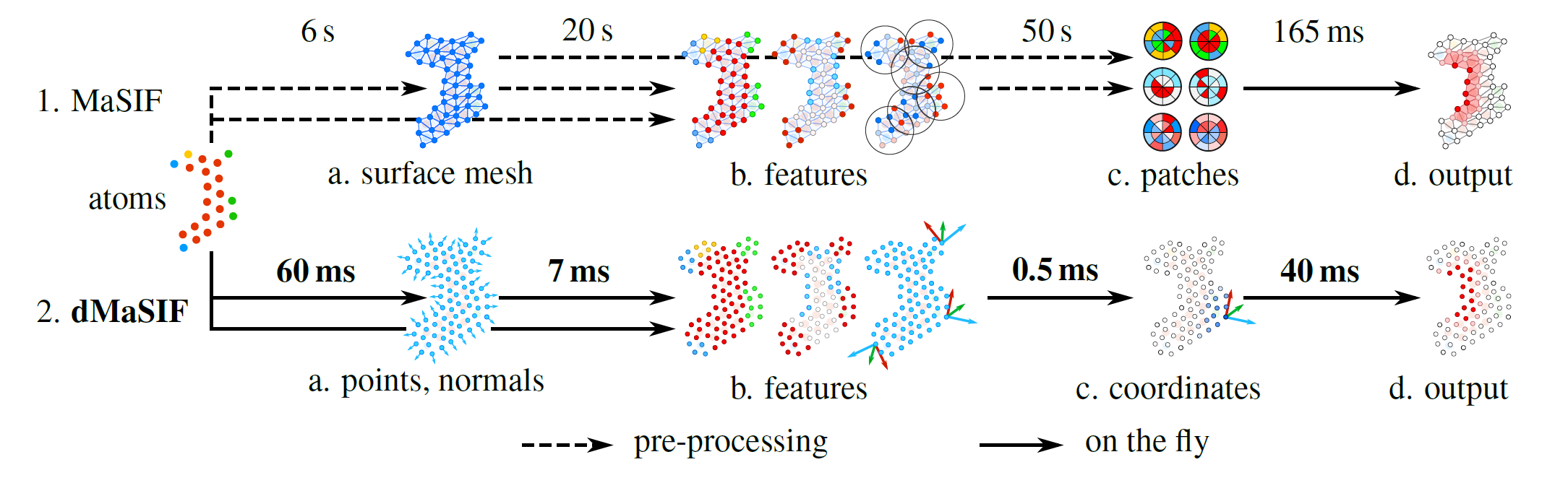
Figure 4: Overview of MaSIF [17] and dMaSIF [70] for binding site prediction. They have similar steps, and each step’s average running time per protein is marked. MaSIF precomputes steps in a-c, whereas dMaSIF computes them on the fly and is 600 times faster than MaSIF.

3.1.3 Datasets

Protein Data Bank (PDB) [122] contains 3D structural protein data obtained by X-ray crystallography, NMR spectroscopy, and cryo-electron microscopy.

Dockground [123] provides a comprehensive set of protein-protein docking complexes extracted from the PDB.

3.1.4 Evaluation Metrics

As there is typically no threshold for the binding site prediction, ROC-AUC is widely used for the evaluation.

3.1.5 Limitations and Future Directions

Although remarkable success has been achieved by applying geometric deep learning for binding site prediction, there are two limitations of existing methods that must be addressed in future research. The first is to predict the binding site conditioned on the binding ligands. Since binding ligands have various biochemical characteristics, such as varying size, polar and hydrophobic groups, binding pockets have specificity to ligands, and it is reasonable to consider ligand information in binding site prediction. The second open question is to predict cryptic pockets that are not apparent in experimentally determined structures. However, caused by protein structural fluctuations [124, 125], ligands can bind to cryptic pockets and modulate protein function via inhibition or activation. Therefore, the ability to accurately and rapidly predict cryptic pockets is an important opportunity to expand the space of druggable proteome. PocketMiner[73] is a pioneering work on cryptic pocket prediction, and we expect to see more research in this area.

3.2 Binding Pose Prediction

3.2.1 Problem Formulation

Predicting the binding mode of a ligand molecule to a target protein, commonly referred to as molecular docking, is a fundamental challenge in drug discovery with a wide range of practical applications. We can represent the target protein structure as $\mathcal{P}$, the ligand’s 2D graph as $G$, and the 3D structure of the ligand as $R$. The primary goal is to develop a model for $p(R|G,\mathcal{P})$ model that can be used to predict the 3D binding pose of the ligand.

3.2.2 Representative Methods

Traditional molecular docking methods rely on manually designed scoring functions and extensive conformation sampling to predict the optimal binding conformation. More recently, this research area has witnessed significant advancements by applying geometric deep-learning techniques, resulting in remarkable progress. One noteworthy progress in this field is EquiBind [35], which marks the first instance of incorporating a geometric deep learning model into the task of molecular docking. Specifically, EquiBind [35] employs an SE(3)-equivariant geometric deep learning model to facilitate direct-shot predictions of both the receptor’s binding site location and the bound pose of the ligand. This is achieved by predicting and aligning key pocket landmarks on the ligand and the protein. In comparative evaluations against traditional methods like VINA [126] and SMINA, EquiBind substantially enhances docking efficiency, outperforming them by orders of magnitude—by a factor ranging from 3 to 5. TANKBind [80] further improves over EquiBind by combining a divide-and-conquer strategy and a Trigonometry-Aware Neural network. TANKBind predicts the inter-molecular distance matrix and then takes a numerical approach to generate specific ligand coordinates based on the inter-molecular distance matrix, coordinates of protein nodes, and the pair distance matrix of ligand nodes. Following in the footsteps of TANKBind, E3Bind [83] uses a divide-and-conquer strategy and designs a trigonometry-aware equivariant graph network to iteratively update the ligand coordinates. This framework can directly predict the coordinates without the employ of a numerical approach-based generation process. Generally, these methods treat the binding pose generation task as a regression problem.

In contrast to the prevalent approach, DiffDock [18] introduces a groundbreaking perspective by framing it as a generative modeling problem (Figure 5). As a diffusion generative model over the non-Euclidean manifold of ligand poses, DiffDock maps the manifold to the product space of the degrees of ligand freedom (translational, rotational, and torsional) involved in docking and develops an efficient diffusion process on this space. The diffusion model generates a set of candidate poses for each input protein-ligand pair, and a trained confidence model is employed to pick out the most likely pose. In scenarios of blind docking, where binding sites are not provided, DiffDock achieves comparable inference efficiency and significant performance improvement over chemoinformatics and geometric deep learning methods.

Generally, previous works predominantly focus on rigid docking, where proteins are considered rigid bodies and the flexibility of protein structures is ignored; it is crucial to acknowledge that protein structures are inherently flexible and can undergo intrinsic or induced conformational changes [127]. Unfortunately, these aspects are overlooked by the methods above. Recent methods, such as NeuralPLexer [81] and DynamicBind [82], consider the flexibility of protein structures, resulting in superior performance in predicting protein-ligand complex structures. NeuralPLexer [81], for instance, incorporates a diffusion model that integrates essential biophysical constraints coupled with a multi-scale geometric deep learning system. This combination enables the iterative sampling of residue-level contact maps and the determination of all heavy-atom coordinates within the protein-ligand complex. Following the path blazed by DiffDock[18], DynamicBind [82] not only considers the degree of ligand freedom (translational, rotational, and torsional) but also takes into account the degree of freedom within protein side chains (torsional). These methods exhibit significant potential for advancing the field of geometric deep learning in dynamic docking scenarios.

TABLE II: Summary of different metrics of representative molecular docking methods on PDBBind dataset for blind docking task. Unless otherwise specified, the default input is assumed to be the holo conformation of the protein. The best results are highlighted in bold.

Method Top-1 Ligand RMSD Top-1 Ligand Centroid Time(s) ($\downarrow$) Percentiles ($\downarrow$) Below threshold ($\uparrow$) Percentiles ($\downarrow$) Below threshold ($\uparrow$) 25th 50th 75th 2 Å 5 Å 25th 50th 75th 2 Å 5 Å VINA [126] 5.7 10.7 21.4 5.5 21.2 1.9 6.2 20.1 26.5 47.1 206 QVINA-W [128] 2.5 7.7 23.7 20.9 40.2 0.9 3.7 22.9 41.0 54.6 10 GNINA [129] 2.4 7.7 17.9 22.9 40.8 0.8 3.7 23.1 40.2 53.6 127 SMINA [130] 3.1 7.1 17.9 18.7 38.0 1.0 2.6 16.1 41.6 59.8 126 GLIDE [131] 2.6 9.3 28.1 21.8 33.6 0.8 5.6 26.9 36.1 48.7 1405 EquiBind [35] 3.8 6.2 10.3 5.5 39.1 1.3 2.6 7.4 40.0 67.5 0.04 TANKBind [78] 2.5 4.0 8.5 20.4 59.0 0.9 1.8 4.4 55.1 77.1 2.5 E3bind [83] 2.1 3.8 7.8 23.4 60.0 0.8 1.5 4.0 60.0 78.8 2.1 DiffDock [18] 1.4 3.3 7.3 38.2 63.2 0.5 1.2 3.2 64.5 80.5 40 DiffDock (Apo) [18] - - - 21.7 - - - - - - 10 NeuralPLexer (Apo) [81] 1.3 2.8 5.9 39.5 69.7 - - - - - 2.1 DynamicBind (Apo) [82] - - - 33.0 65.0 - - - - - -

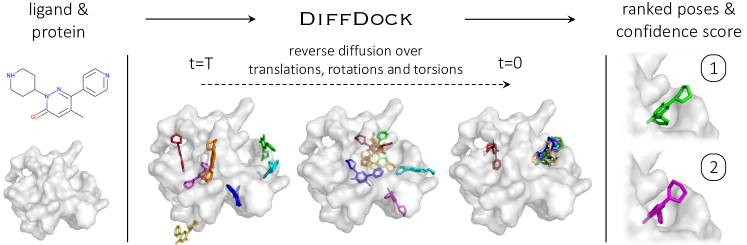
Figure 5: Overview of DiffDock [18] for binding pose prediction. The model takes as input the separate ligand and protein structures. Randomly sampled initial poses are denoised via a reverse diffusion process over translational, rotational, and torsional degrees of freedom. A trained confidence model ranks the sampled poses to produce a final prediction and confidence score.

3.2.3 Datasets

PDBBind [132] is a subset of the PDB [133] that contains experimentally measured 3D structures of protein-ligand complexes. The newest version, PDBBind v2020, contains 19,443 protein-ligand complexes with 3,890 unique receptors and 15,193 unique ligands. This dataset is often used for molecular docking tasks. Nevertheless, while nearly all geometric deep learning methods are trained on this dataset, variations exist in the detailed settings, as outlined in Table IV.

3.2.4 Evaluation Metrics

Centroid Distance calculates the distance between the averaged coordinates of the predicted and truly bound ligand atoms.

Ligand Root Mean Square Deviation (L-RMSD) is the mean squared error between the atoms of the predicted and bound ligands. Formally, let $R\in\mathbb{R}^{n\times 3}$ and $\hat{R}\in\mathbb{R}^{n\times 3}$ be the predicted and the ground truth ligand coordinates, where $n$ is the number of atoms. The L-RMSD is obtained with:

$$\text{L-RMSD}(R,\hat{R})=\big{(}\frac{1}{n}\sum_{i=1}^{n}||R_{i}-\hat{R}_{i}||^{2}\big{)}^{\frac{1}{2}},$$ (18)

where $R_{i}$ and $\hat{R}_{i}$ denote the coordinate of the $i$-th atom.

Kabsch RMSD is the lowest possible RMSD that the roto-translation transformation of the ligand can obtain. It first uses the Kabsch algorithm to superimpose the two structures and then calculates the RMSD score similar to Equation. 18.

PoseBusters [134] is a novel test suite designed to assess the chemical and physical plausibility of ligand poses, complementing accuracy-based metrics like RMSD. The PoseBusters test suite consists of 18 checks in total, organized into three groups of tests to evaluate chemical, intramolecular, and intermolecular validity.

3.2.5 Benchmark Performance

In Table II, the performance of selected molecular docking methods is displayed. NeuralPLexer and DynamicBind focus on dynamic docking, while the remaining methods address rigid docking. Dynamic docking methods use the apo conformation of proteins, and rigid docking methods apply the holo conformation. The table indicates that DiffDock performs well in rigid docking, and NeuralPLexer is effective in dynamic docking scenarios.

3.2.6 Limitations and Future Directions

Ever since EquiBind [35] pioneered the incorporation of geometric deep learning into molecular docking tasks, a series of geometric deep learning-based docking methods have emerged. Although these methods exhibit notable enhancements in the RMSD metric for blind docking tasks, they face challenges in generating physically plausible ligand poses. Research by Buttenschoen et al.[134] demonstrate that even for data with RMSD less than 2.0 Å predicted by DiffDock, only 36.8% of the data represents physically plausible ligand poses (Table III), with steric clashes between the protein and ligand being a prevalent issue. These findings underscore the ongoing challenge for geometric deep-learning models to generate accurate and physically plausible ligand poses. What’s more, the recent development of GPU-accelerated sampling methods, such as VINA-GPU [135] and DSDP [136], achieve significant acceleration in speed. Analyses suggest that current molecular docking has no efficiency advantage and fails to predict physically valid poses. Thus, in the future, it will be imperative to expand more intrinsic advantages of geometric deep learning models, such as considering the protein side chain’s flexibility.

TABLE III: Summary of different metrics of representative molecular docking methods on PoseBuster [134] dataset for blind docking task. Data points pass all PoseBuster tests and are denoted as ”PB-Valid”.

Method	$\%$ RMSD $\leq$ 2.0 Å	$\%$ RMSD $\leq$ 2.0 Å (PB-Valid)
VINA [137]	52	51
EquiBind [35]	2.6	0.0
TANKBind [78]	15	2.6
DiffDock [18]	38	14

TABLE IV: Datasets used by geometric deep learning-based molecular docking methods.

Method	Training and validation sets
EquiBind [35], E3Bind [83], DiffDock [18]	PDBbind 2020 General Set with complexes published before 2019 and without those with ligands found in the test set—17,347 complexes in total.
TankBind [78], DynamicBind[82]	PDBbind 2020 General Set with complexes published before 2019 and without those failing pre-processing—18,755 complexes in total.
NeuralPlexer [81]	Constructing a new dataset, PL2019-74k, based on the PDB accessed in April 2022. PL2019-74k is obtained by removing samples deposited after January 2019 and samples with UniProt ID in the PocketMiner dataset, resulting in 74,477 samples for model training.

TABLE V: Training setting, testing setting, and test performance of binding affinity prediction models.

Method Year Training set Testing set RMSE ($\downarrow$) PCC ($\uparrow$) Pafnucy [96] 2018 PDBbind v2016 general set (N=11,906) PDBbind v2016 core set (N=290) 1.420 0.780 DeepAtom [97] 2019 PDBbind v2016 refined set (N=3,390) PDBbind v2016 core set (N=290) 1.318 0.807 OnionNet [138] 2019 PDBbind v2016 general set (N=11,906) PDBbind v2016 core set (N=290) 1.287 0.816 PIGNet [86] 2021 PDBbind v2019 refined augment set (N=1,656,600) PDBbind v2016 core set (N=283) - 0.749 Fusion [101] 2021 PDBbind v2016 general set (N=-) PDBbind v2016 core set (N=290) 1.270 0.820 OnionNet-2 [139] 2021 PDBbind v2019 general set (N=17,367) PDBbind v2016 core set (N=285) 1.164 0.864 IGN [90] 2021 PDBbind v2016 general set (N=8,298) PDBbind v2016 core set (N=262) 1.220 0.837 SIGN [21] 2021 PDBbind v2016 refined set (N=3,390) PDBbind v2016 core set (N=290) 1.316 0.797 PLIG [88] 2022 PDBbind v2020 general set + PDBbind v2016 refined set (N=19,451) PDBbind v2016 core set (N=285) 1.210 0.840 PaxNet [89] 2022 PDBbind v2016 refined set (N=3,390) PDBbind v2016 core set (N=290) 1.263 0.815 GLI [140] 2022 PDBbind v2016 refined set (N=3,390) PDBbind v2016 core set (N=290) 1.294 - GIGN [91] 2023 PDBbind v2016 general set (N=11,906) PDBbind v2016 core set (N=290) 1.190 0.840 KIDA [100] 2023 PDBbind v2016 general set (N=12,500) PDBbind v2016 core set (N=285) 1.291 0.837 GraphscoreDTA [92] 2023 PDBbind v2019 general set (N=9,869) PDBbind v2016 core set (N=279) 1.249 0.831 PLANET [93] 2023 PDBbind v2020 general set (N=15,616) PDBbind v2016 core set (N=285) 1.247 0.824 MBP [95] 2023 PDBbind v2016 refined set (N=3,390) PDBbind v2016 core set (N=290) 1.263 0.825

3.3 De Novo Ligand Generation

3.3.1 Problem Formulation

The goal of de novo ligand generation is to generate valid 3D molecular structures that can fit and bind to specific protein binding sites. De novo generation involves generating a molecule while no reference ligand molecule is given, i.e., developing molecules from scratch. Formally, let $\mathcal{P}$ denote the protein structure and $\mathcal{G}$ be the 3D ligand molecule. The objective is to learn a conditional generative model $p(\mathcal{G}|\mathcal{P})$ to capture the distribution of protein-ligand pairs.

3.3.2 Representative Methods

Early methods on de novo ligand generation represent the target protein as a 3D grid and employ 3D CNN as the encoder. For example, LiGAN [141] uses a conditional variational autoencoder trained on atomic density grid representations of protein-ligand structures for ligand generation. The molecular structures of ligands are then constructed by further atom fitting and bond inference from the generated atom densities. However, as a preliminary work, LiGAN does not satisfy the desirable equivariance property.

The follow-up methods represent the target protein and ligand as 3D graphs/point clouds, and the equivariance is achieved by leveraging equivariant GNNs for context encoding. For example, 3DSBDD [142] uses SchNet [143] to encode the 3D context of binding sites and estimate the probability density of atom’s occurrences in 3D space. The atoms are sampled auto-regressively until there is no room for new atoms. GraphBP [144] adopts the framework of normalizing flow [145] and constructs local coordinate systems to predict atom types and relative positions.

Pocket2Mol [19] adopts the geometric vector perceptrons [146] and the vector-based neural network [147] as the context encoder. Inspired by AlphaFold [7] for protein structure prediction, Pocket2Mol incorporates a triangular self-attention in the encoder, where the attention bias is designed to capture the geometric constraints. Pocket2Mol jointly predicts frontier atoms, atomic positions, atom types, and covalent chemical bonds. With vector-based neurons, Pocket2Mol can efficiently sample drug molecules from tractable distributions without relying on MCMC.

By leveraging the chemical priors of molecular fragments such as functional groups, FLAG [69] and DrugGPS [108] propose to generate ligand molecules fragment-by-fragment and yield more realistic substructures. For example, in FLAG [69], a motif vocabulary is firstly constructed by preprocessing the dataset and extracting molecular fragments with high occurrence frequencies (i.e., motif). Drug molecules are constructed auto-regressively in the generation process with motifs as the building blocks. At each generation step, as shown in Figure 6, a 3D graph neural network encodes the intermediate context information, selects the focal motif, predicts the next motif type, and attaches the new motif to the generated molecule. Since the bond lengths/angles are largely determined, FLAG leverages cheminformatics tools [148] to effectively determine them and focus on training neural networks for rotation angle prediction.

Building based on FLAG [69], DrugGPS [108] further considers the generalizability issue of structure-based drug design models: the amount of high-quality protein-ligand complex data is rather limited and the target protein pocket may not be in the training dataset. The trained model struggles to generate good drug candidates for the unseen target protein. DrugGPS[108] effectively incorporates the protein subpocket prior to generalizable drug molecule generation. Although two protein pockets might be dissimilar overall, they may still bind the same fragment if they share similar subpockets [149]. To capture the subpocket-level similarities/invariance among the binding pockets, DrugGPS[108] proposes to learn subpocket prototypes and construct a global interaction graph to model the subpocket prototype-molecular motif interactions during training.

Recently, motivated by the powerful generation capability of the Diffusion models, Diffusion-based methods such as DiffSBDD [1], TargetDiff [114], and DecompDiff [116] are proposed for non-autoregressive ligand generation and achieve superior performance. For example, TargetDiff [114] learns a joint drug molecule generative process of both continuous atom coordinates and categorical atom types with an SE(3)-equivariant network conditioned on the protein pocket. Further studies show that TargetDiff [114] can also extract representative features from protein-ligand complexes to estimate the binding affinity, providing an effective virtual screening method. Inspired by pharmaceutical practices, DecompDiff [116] considers different roles of atoms in the ligand and decomposes the ligand molecule and prior into two parts, namely arms and scaffold for drug design. The arms are responsible for the interactions with the binding regions for higher affinity, whereas the scaffold’s role involves placing the arms accurately within the intended binding regions. Moreover, DecompDiff [116] incorporates both bond diffusion in the model and additional validity guidance in the sampling phase to improve the properties of the generated molecules.

TABLE VI: Comparison of the properties of the reference molecules and the generated molecules by different de novo ligand generation methods. Vina Score indicates the Vina scoring function is directly calculated without ligand redocking or local optimization. Vina Min denotes that the ligand is locally minimized. Vina Dock indicates the ligand is locally optimized and redocked.

Vina Score ($\downarrow$) Vina Min ($\downarrow$) Vina Dock ($\downarrow$) High Affinity ($\uparrow$) QED ($\uparrow$) SA ($\uparrow$) Diversity ($\uparrow$) Avg. Med. Avg. Med. Avg. Med. Avg. Med. Avg. Med. Avg. Med. Avg. Med. Reference -6.36 -6.46 -6.71 -6.49 -7.45 -7.26 - - 0.48 0.47 0.73 0.74 - - liGAN [103] - - - - -6.33 -6.20 21.1% 11.1% 0.39 0.39 0.59 0.57 0.66 0.67 GraphBP [110] - - - - -4.80 -4.70 14.2% 6.7% 0.43 0.45 0.49 0.48 0.79 0.78 3DSBDD [2] -5.75 -5.64 -6.18 -5.88 -6.75 -6.62 37.9% 31.0% 0.51 0.50 0.63 0.63 0.70 0.70 Pocket2Mol [19] -5.14 -4.70 -6.42 -5.82 -7.15 -6.79 48.4% 51.0% 0.56 0.57 0.74 0.75 0.69 0.71 TargetDiff [114] -5.47 -6.30 -6.64 -6.83 -7.80 -7.91 58.1% 59.1% 0.48 0.48 0.58 0.58 0.72 0.71 FLAG [69] -5.30 -5.89 -6.46 -6.68 -7.25 -7.17 53.7% 54.8% 0.50 0.51 0.75 0.72 0.70 0.73 DrugGPS[108] -5.45 -5.81 -6.49 -6.88 -7.36 -7.42 54.9% 55.7% 0.59 0.58 0.72 0.73 0.71 0.74 Decompdiff[116] -5.67 -6.04 -7.04 -7.09 -8.39 -8.43 64.4% 71.0% 0.45 0.43 0.61 0.60 0.68 0.68

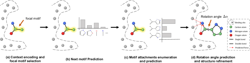
Figure 6: Overview of FLAG [69] for de novo ligand generation. There are four steps in each iteration: (a) context encoding and focal motif selection, (b) next motif prediction, (c) motif attachments enumeration and prediction, and (d) rotation angle prediction and structure refinement.

3.3.3 Datasets

CrossDocked dataset [150] is widely used in structure-based de novo ligand design [2, 19], which contains 22.5 million protein-molecule structures by cross-docking the Protein Data Bank [122]. Considering the variability in the cross-docked complex qualities, existing methods typically employ filtering steps. After filtering out data points whose binding pose RMSD is greater than 1 Å, a refined subset with around 180,000 data points is obtained. For the dataset split, mmseqs2 [151] is widely used to cluster data at 30$\%$ sequence identity, 100,000 protein-ligand pairs are randomly drawn for training and 100 proteins from the remaining clusters for testing. One hundred molecules for each protein pocket in the test set are sampled to evaluate generative models.

Binding MOAD [152] contains experimentally determined complexed protein-ligand structures. The dataset is filtered and split based on the proteins’ enzyme commission number [153]. Specifically, the split ensures different sets do not contain proteins from the same Enzyme Commission Number (EC Number) main class. Finally, there are 40,354 protein-ligand pairs for training and 130 for testing.

3.3.4 Evaluation Metrics

The following metrics are widely used in related works [2, 19, 144, 108, 69] to evaluate the qualities of the sampled molecules: (1) Validity is the percentage of chemically valid molecules among all generated molecules. A molecule is valid if it can be sanitized by RDkit [148]. (2) Vina Score measures the binding affinity between the generated molecules and the protein pockets. It can be calculated with traditional docking methods such as AutoDock Vina [137, 154] or trained CNN scoring functions [155]. Before calculating the vina score, the generated molecular structures are refined by universal force fields [156]. (3) High Affinity is calculated as the percentage of pockets whose generated molecules have higher affinity to the references in the test set. (3) QED measures how likely a molecule is a potential drug candidate. (4) Synthetic Accessibility (SA) indicates the difficulty of drug synthesis (the score is normalized between 0 and 1, and higher values indicate more accessible synthesis). (5) LogP is the octanol-water partition coefficient (LogP values should be between -0.4 and 5.6 to be promising drug candidates [157]). (6) Lipinski (Lip.) calculates how many rules the molecule obeys the Lipinski’s rule of five [158]. (7) Sim. Train represents the Tanimoto similarity [159] with the most similar molecules in the training set. (8) Diversity (Div.) measures the diversity of generated molecules for a binding pocket (It is calculated as 1 - average pairwise Tanimoto similarities). (9) Time records the cost of generating 100 valid molecules for a pocket.

3.3.5 Bechmark Performance

We benchmark representative de novo ligand generation methods on the CrossDocked dataset in Table VI. Generally, there is not a single method that is optimal on all the metrics. We can observe that diffusion-based methods achieve the best performance on binding affinity (Vina-related metrics). This may be attributed to their non-autoregressive generation scheme that facilitates global optimization. As for QED and SA, fragment-based methods such as DrugGPS achieve the most competitive performance. This may be explained by incorporating drug-like fragments, effectively increasing drug-likeliness and synthesizability.

3.3.6 Limitations and Future Directions

Despite the success of applying geometric deep learning for de novo ligand generation, it is still challenging to explore the vast chemical space and generate high-quality drug candidates with satisfied properties. Generally, current methods have the following limitations and require further explorations: (1) failing to consider essential chemical priors; (2) lacking ligand optimization methods; (3) noncomprehensive evaluation metrics.

Firstly, most current methods fail to consider essential chemical priors such as molecular motifs and protein-ligand interaction patterns. Therefore, the generated ligand molecules may have invalid 3D structures and limited binding affinity with the target protein. FLAG [69] and DrugGPS [108] have tried to leverage chemical priors of motifs and subpockets in the model construction. In the future, we expect more methods that leverage the chemical priors for high-quality ligand generation.

Secondly, existing works fail to explicitly optimize drug properties in the generation process. In practice, it is challenging to directly generate drug candidates satisfying a series of property constraints. A common practice is sampling promising lead compounds and then conducting lead optimization. Therefore, exploring multiple-property optimization methods for de novo ligand generation is one future direction.

Thirdly, the current evaluation metrics are noncomprehension, and most focus on 2D molecule properties such as QED and SA. A recent work, PoseCheck [160], proposes four metrics to evaluate the generated molecules’ poses, including interaction profiles, steric clashes, strain energy, and redocking RMSD. Their evaluations show that the ligand molecule generated by existing methods often exhibits nonphysical features such as steric clashes, hydrogen placement issues, and high strain energy. In the future, we expect more comprehensive evaluation metrics and more advanced ligand generative models that address the shortcomings.

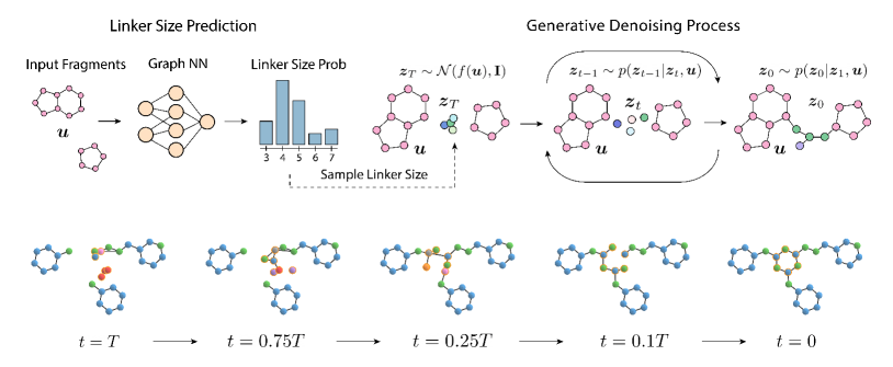
Figure 7: Overview of DiffLinker [121] for linker design. The inputs are the molecular fragments and the protein pocket (optional). The output is the linker that links the fragments into a complete molecule. DiffLinker is an E(3)-equivariant diffusion-based model. In the generation process, the probabilities of linker sizes are first computed for the input fragments. Next, linker atoms are sampled and denoised using a conditioned equivariant diffusion model. The bottom shows the linker generation process with linker atoms highlighted in orange.

3.4 Linker Design

3.4.1 Problem Formulation

Most small molecular drugs bind to the target protein and inhibit its activity. However, due to the complexity of diseases, some amino acids in target proteins may mutate, leading to weak binding affinity and drug falling off. To solve this problem, an emerging therapeutic mechanism involving proteolysis targeting chimera (PROTAC) can inhibit protein functions by prompting complete degradation of the target protein. Specifically, PROTAC contains two molecular fragments and a linker that links the fragments into a complete molecule. One fragment in PROTAC binds the target protein and the other fragment binds another molecule that can degrade the target protein. Because PROTAC only requires high selectivity in binding its targets instead of inhibiting the target protein’s activity, much attention is focused on repurposing previously ineffective inhibitor molecules as PROTAC for the next generation of drugs. One critical problem in PROTAC is linker design, which generates the linker conditioned on the given fragments and the target protein. Formally, denote the target protein as $\mathcal{P}$, the molecular fragments as $\mathcal{F}$, and the linker as $\mathcal{L}$; the objective is to learn a conditional generative model $p(\mathcal{L}|\mathcal{F,P})$.

TABLE VII: Linker design performance comparisons on the ZINC test sets. Given anchors denotes that the anchors are known to the model. Sampled size indicates the linker size is sampled and is not necessarily the same as the ground truth.

Model QED ($\uparrow$) SA ($\uparrow$) Valid ($\uparrow$) Unique ($\uparrow$) Novel ($\uparrow$) DeLinker[118] 0.64 0.77 98.3% 44.2% 47.1% 3DLinker [20] (given anchors) 0.65 0.77 99.3% 29.0% 41.2% 3DLinker [20] 0.65 0.76 71.5% 29.2% 41.9% DiffLinker [121] 0.68 0.78 93.8% 24.0% 30.3% DiffLinker [121] (given anchors) 0.68 0.77 97.6% 22.7% 32.4% DiffLinker [121] (sampled size) 0.65 0.76 90.6% 51.4% 42.9% DiffLinker [121] (given anchors, sampled size) 0.65 0.76 94.8% 50.9% 47.7%

3.4.2 Representative Methods

DeLinker [118] uses VAE and autoregressively generates the atoms and edges of the linker. Only simple geometric information, such as the relative distances and orientations, is considered in DeLinker, and the output is the 2D molecule graph. 3Dlinker [20] also generates linker autoregressively but can further generate the 3D molecule structure without specifying the anchor atoms, i.e., the atoms of fragments for linking. The anchor node, next node type, edge, and coordinate are predicted sequentially in each step.

Link-INVENT [120] and PROTAC-INVENT [66] are reinforcement learning-based methods. Link-INVENT [120] expands the widely used REINVENT [161] model and incorporates a reward function to optimize the length, linearity, and flexibility of generated linkers. However, Link-INVENT [120] only focuses on 2D linker generation. PROTAC-INVENT [66] can jointly sample the 2D molecular graphs and the 3D structures of linkers inside the target protein pocket.

DiffLinker [121] designs a conditional diffusion-based model that generates molecular linkers conditioned on input fragments and the target protein structure (optional). In the generation process (Figure 7), the probabilities of linker sizes are first computed for the input fragments. Next, linker atoms are sampled and denoised using a conditioned equivariant diffusion model. Results show that considering the target protein structure improves the binding affinity of the resulting PROTAC molecules.

3.4.3 Datasets

Zinc [162] is a free database of commercially-available compounds for virtual screening. A subset of 250,000 molecules randomly selected by [163] is used for linker design. The dataset is preprocessed as follows: firstly, 3D conformers are generated using RDKit [148], and a reference 3D structure with the lowest energy conformation is selected for each molecule. Then, these molecules are fragmented by enumerating all double cuts of acyclic single bonds outside functional groups. The results are further filtered by the number of atoms in the linker and fragments, synthetic accessibility [164], ring aromaticity, and pan-assay interference compounds (PAINS) [165] criteria. As a result, a single molecule may yield different combinations of two fragments separated by a linker. The Zinc dataset is randomly split into train, validation, and test sets (438,610/400/400 examples).

CASF [166] includes experimentally verified 3D conformations. The preprocessing procedure is the same as Zinc.

GEOM [167] is considered for real-world applications that require connecting more than two fragments with one or more linkers. The molecules are decomposed into three or more fragments with one or two linkers with an MMPA-based algorithm [168] and BRICS [169].

Binding MOAD [152] contains experimentally determined complexed protein-ligand structures. DiffLinker [121] uses Binding MOAD to assess further the ability to generate valid linkers given additional information about protein pockets. The authors extract amino acids with at least one atom closer than 6 Å to any ligand atom as the pockets. The molecules are preprocessed into fragments using RDKit’s implementation of MMPA-based algorithm [168]. The resulting dataset is split based on the proteins’ Enzyme Commission (EC) numbers.

3.4.4 Evaluation Metrics

The following metrics are widely used to evaluate linker design methods: (1) Validity is the percentage of chemically valid molecules among all generated molecules. (2) Quantitative Estimation of Drug-likeness (QED) measures how likely a molecule is a potential drug candidate. (3) Synthetic Accessibility (SA) indicates the difficulty of drug synthesis. (4) Rings is the average number of rings in the linker. (5) Uniqueness measures the percentage of non-duplicate generated molecules. (6) Novelty calculates the ratio of generated molecules not in the training set. (7) Recovery records the percentage of the original molecules recovered by the generation process. (8) Root Mean Squared Deviation (RMSD) is calculated between the generated and real linker coordinates in the cases where true molecules are recovered. (9) $\rm RD_{scit}$ [170] evaluates the geometric and chemical similarity between the ground truth and generated molecules.

3.4.5 Benchmark Performance

We benchmark representative linker design methods on the Zinc dataset in Table VII. In the default setting, all the methods generate the linker the same size as the ground truth. DiffLinker [121] as the state-of-the-art method achieves the best results on molecule drug-likeliness and synthesizability. We also note that sampling the linker size can significantly improve novelty and uniqueness of the generated linkers without much degradation of the other important metrics.

3.4.6 Limitations and Future Directions

Although impressive progress has been obtained for linker design with geometric deep learning, there remain open questions. Firstly, most existing methods fail to consider the protein pocket context. The generated molecules may have steric clashes or inferior binding affinities with the target protein. We are glad to see some recent methods, such as DiffLinker [121], manage to design linkers conditioned on the pocket and expect to see more progress in this direction. Secondly, existing models for linker design assume that the relative positions of the fragments are known, which may not be practical in real scenarios. Generative models that co-design both fragment poses and linkers are more favorable.

3.5 Binding Affinity Prediction

3.5.1 Problem Formulation

Protein-ligand binding affinity is a measurement of interaction strength. Accurate affinity prediction helps design effective drug molecules and plays a vital role in SBDD. Formally, denoted the bound protein structure as $\mathcal{P}$, the bound ligand as $\mathcal{L}$, and the binding affinity as $y$, our target is to train a model $f(\mathcal{P},\mathcal{L})=y$ for binding affinity prediction.

3.5.2 Representative Methods

The exploration of binding affinity prediction methods has a long-standing history. Early studies focused on utilizing empirical formulas [171] or designing handcrafted features coupled with traditional machine learning algorithms for binding affinity prediction [172]. Despite some advancements, these methods have limited prediction accuracy and require considerable feature engineering to perform well. Recent research has highlighted the application of geometric deep learning methods, representing the protein-ligand complex structure as 3D grids or 3D graphs for processing and prediction. These approaches directly model the relationship between the complex’s 3D structure and binding affinity using CNNs or GNNs. For example, given a complex structure, Pafnucy [96] extracts a 20 Å cubic box focused on the geometric center of the ligand and discretizes it into a $21\times 21\times 21\times 19$ grid with 1 Å resolution. A 3D-CNN is then employed to process the grid, treating it as a multi-channel 3D image. SIGN [21] converts the complex structure into a complex 3D graph and designs a structure-aware interactive graph neural network to capture 3D spatial information and global long-range interactions using polar-inspired graph attention layers in a semi-supervised manner. PIGNet [86] introduces a novel physics-informed graph neural network, which can predict accurate binding affinity based on four physics energy components – van der Waals (vdW) interaction, hydrogen bond, metal-ligand interaction, and hydrophobic interaction (Figure 8). Fusion [101] simultaneously utilizes the complex 3D grid representation and 3D graph to capture different characteristics of interactions. HOLOPROT [87] considers both complex structures and complex surfaces. MBP [95] introduces the first affinity pre-training framework, which involves training the model to predict the ranking of samples from the same bioassay. This pre-training uses a self-constructed ChEMBL-Dock dataset containing over 300,000 experimental affinity labels and about 2.8M docking-generated complex structures. The geometric deep learning-based methods effectively capture the 3D structural information and show superior prediction accuracy.

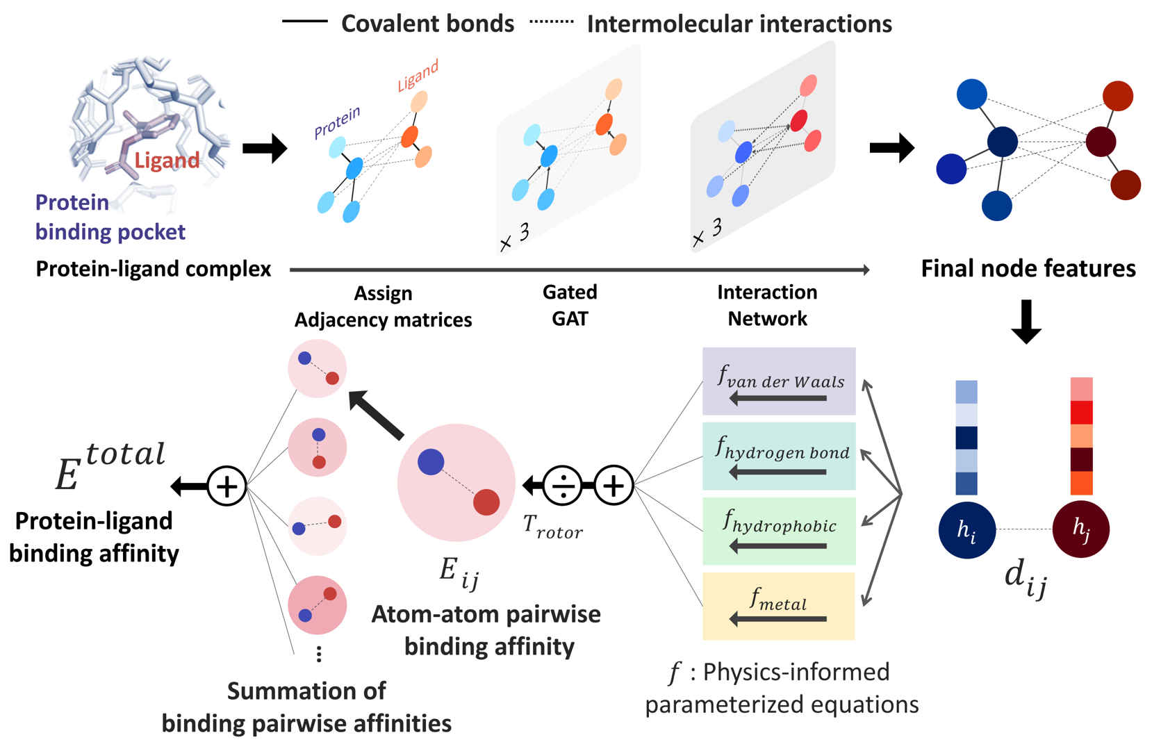
Figure 8: Overview of PIGNet [86] for binding affinity prediction. A protein-ligand complex is represented in a graph, and adjacency matrices are assigned from the binding structure of the complex. Each node feature is updated through neural networks to carry the information of covalent bonds and intermolecular interactions. Given each atom pair’s distance and final node features, four energy components are calculated from the physics-informed parameterized equations. The total binding affinity is obtained as a sum of pairwise binding affinities, a sum of the four energy components divided by an entropy term.

3.5.3 Datasets

PDBBind [132] is the most commonly used dataset for binding affinity prediction. As previously mentioned, the latest version of the dataset consists of 19,443 complexes. Specifically, the dataset comprises three overlapping subsets: the general set (14,127 3D protein-ligand complexes), the refined set (5,316 complexes selected from the general set with higher quality), and the core set (290 complexes selected as the highest quality benchmark for testing). It is customary to train and validate models on either the general or refined sets and evaluate them on the core set. The PDBbind v2016 core set is also known as the CASF-2016 dataset.

CSAR-HiQ [173] is another commonly used dataset, consisting of two subsets containing 176 and 167 complexes, respectively. This dataset is often used as the independent dataset in generalizability benchmarks.

3.5.4 Evaluation Metrics

Root Mean Square Error (RMSE) and Mean Absolute Error (MAE) are widely used to quantify the errors between the predicted values and the ground-truth values [174]. These two metrics are the most direct evaluation metrics for prediction errors.

Pearson’s Correlation Coefficient (PCC) [175] quantifies the linear correlation between the predicted values and the ground-truth values. This metric serves as a means to evaluate prediction accuracy. Unlike RMSE and MAE, PCC is a normalized value ranging from -1 to 1, allowing for a standardized assessment of prediction accuracy.

Spearman’s Correlation Coefficient (SCC) [176] quantifies the ranking correlation between predicted values and experimental values. It is calculated as the PCC between the rank values of the two variables. This metric is relevant, as affinity prediction is frequently employed to identify molecules with the highest rankings in virtual screening.

3.5.5 Benchmark Performance

The field of affinity prediction methods has a rich history, characterized by various methodologies and the utilization of diverse datasets. Consequently, conducting a fair and comprehensive comparison of all these methods presents a formidable challenge. In Table V, we present statistics on training and testing settings and the performance of these binding affinity prediction models. As shown in the table, although the testing settings of these methods are generally the same, their training settings vary significantly. Larger training datasets generally lead to better results. For future research in binding affinity prediction, it is essential to carefully select suitable settings for training and testing.

3.5.6 Limitations and Future Directions

While recent advancements in geometric deep learning for affinity prediction have significantly improved accuracy, several critical limitations remain to be addressed. Firstly, the current geometric deep learning methods are predominantly trained on co-crystal complex structures where all the data are positive, making it challenging for these methods to effectively screen out true active ligands from a large pool of decoys. As exemplified by PIGNet, previous research has aimed to enhance both the scoring power and the screening power of affinity prediction models. Nevertheless, their results suggest that improving screening power often results in a trade-off with reduced scoring power, underscoring the difficulty of simultaneously achieving high performance in both aspects. It is essential to develop robust models capable of excelling in scoring and screening, expanding their practical applications.

Furthermore, generalization to protein structures beyond those encountered during training is crucial. One potential solution to this challenge involves creating additional high-quality training datasets. Currently, there are approximately 5,000 high-quality protein-ligand complexes with experimentally verified affinities, as the PDBBind refined set exemplifies. However, this limited dataset often constrains the full training of deep learning models. Additionally, integrating prior physical knowledge into deep learning models, such as physics-informed deep learning [177], represents a promising avenue for enhancing generalization capabilities.

4 Challenges and Opportunities

We discuss challenges and opportunities in SBDD across various dimensions, including algorithmic innovation, practical considerations concerning model and output evaluation, and integration with experimental systems.

4.1 Challenges

• Oversimplified Problem Formulation: In structure-based drug design (SBDD), problem formulations must align with real-world applications and adhere to established physical and chemical principles. For instance, numerous studies on binding pose generation and de novo ligand generation operate under the assumption that the target protein structure remains static. In reality, protein structures exhibit flexibility and can experience intrinsic or induced conformational alterations [127]. This discrepancy underscores a gap between SBDD models and their practical applications.

• Out-of-distribution Generalization: Most existing studies do not sufficiently address the out-of-distribution challenge. Given the constraints posed by dataset sizes and, occasionally, inappropriate dataset splits, certain studies might overestimate the efficacy of model predictions. For instance, during the COVID-19 pandemic, generative models need to produce ligand molecules for novel protein targets, such as the main protease of SARS-CoV-2. Consequently, the need for generalizable geometric deep learning models becomes evident, especially for real-world applications.

• The Need for Reliable Evaluation Metrics: Establishing robust criteria to define an optimal drug candidate remains challenging. Even though various evaluation metrics have been proposed, they often fall short in their applicability. Some models exploit shortcuts [178] in these metrics, resulting in the generation of molecules with limited real-world utility.

• Lack of Large-scale Benchmarks: While datasets and evaluation splits are available for diverse SBDD tasks, there remains a dearth of large-scale, reliable benchmarks with high-quality data. For example, the refined dataset from PDBbind [132] used in training affinity prediction models encompasses merely 5,000 complexes. The CrossDocked dataset [150], used to benchmark de novo ligand design methods, comprises only 2,922 distinct proteins and 13,780 unique ligand molecules. These datasets pale compared to the size of chemical space and protein universe, underscoring the need for expansive, high-quality benchmarks.

• The Need for Experimental Verification: Computationally evaluating generated drug candidates using a set of metrics, while valuable, is not sufficient. Experimental verification using in vivo or in vitro tests is crucial to validate a candidate’s effectiveness. These experimental outcomes can be harnessed to refine the models, facilitating an integrative loop between computational simulations and empirical experiments.

• Lack of Interpretability: Achieving interpretability is a paramount yet formidable task for deep learning models, often perceived as black boxes. Within SBDD, researchers often seek insights into rationales behind predicted protein-ligand affinities or factors that can explain why a specific protein surface region represents a viable binding site. While the interpretability of SBDD models aids in debugging and model enhancement, current efforts in this direction, such as those outlined in [72, 179, 180], remain in their infancy and warrant further exploration.

4.2 Opportunities

• Leverage Multimodal Datasets: High-quality protein structure data remains limited; for example, CrossDocked and PDBBind datasets contain fewer than 10 thousand unique protein structures. In contrast, UniRef [181] boasts over 260 million protein sequences. As such, the incorporation of protein language models [182, 183, 184] trained on protein sequence data into structure-based drug design holds promise [185]. Additionally, textual data describing protein functions [186] and proteomics [187] can be integrated into SBDD models.

• Incorporate Biological and Chemical Knowledge: Integrating chemical and biomedical knowledge into model development has proven effective across various tasks. For instance, geometric symmetry is incorporated in equivariant neural networks, while molecular fragments are utilized to generate more realistic and valid molecules. Geometric deep learning stands to gain from the further infusion of domain knowledge.

• Build Comprehensive Benchmarks: Standardized benchmarks offer dataset splits and evaluation tools, facilitating straightforward and robust comparison of SBDD models within a consistent framework [188, 189].

• Design Criteria Based on Clinical Endpoints: Structure-based drug design is considered during the early stages of drug discovery and development. However, a palpable chasm exists between early-phase drug discovery and pre-clinical and clinical drug development [190, 191]. This can result in drug candidates faltering in clinical trials. Consequently, leveraging feedback from late drug development and using it to design novel design criteria to guide SBDD may increase therapeutic yield.

• Establish Foundation Models for SBDD: Contemporary research on geometric deep learning methods for SBDD predominantly revolves around single-task models. However, with the emergence of general-purpose pre-trained models[192, 193, 194, 195], there is potential to develop unified foundation models that are compatible with a variety of data formats and tasks in SBDD.

• Consider a Broad Range of Design Tasks: This survey examines geometric deep learning methods tailored for SBDD tasks, emphasizing small molecule drugs. Many methods are broadly applicable and can be adapted to other areas, such as antibody design [196], protein pocket design [197], and crystal material generation [198].

5 Conclusion

We systematically review geometric deep learning methods and applications for structure-based drug design. Our methodology involves categorizing existing research into five distinct categories based on the tasks they address. We present a comprehensive problem formulation for each task, summarizing noteworthy methods and delineating datasets and evaluation metrics. Considering both challenges and prospects for the field, we anticipate that this survey will facilitate a rapid comprehension of existing methodology and lay the groundwork for future structure-based drug design using geometric deep learning.

Zaixi Zhang received the BS degree from the Department of Gifted Young, University of Science and Technology of China (USTC), China, in 2019. He is currently working toward a Ph.D. degree in the School of Computer Science and Technology at USTC. His main research interests include graph representation learning and AI for Drug Discovery. He has published papers in referred conferences and journals, such as ICML, NeurIPS, CVPR, ICLR, and TKDE.

Jiaxian Yan is a master’s student at School of Data Science, University of Science and Technology of China (USTC). His research interests include data mining and AI-driven drug design.

Qi Liu received the Ph.D. degree from University of Science and Technology of China (USTC), Hefei, China, in 2013. He is currently a Professor in the School of Computer Science and Technology at USTC. His general area of research is data mining and knowledge discovery. He has published prolifically in refereed journals and conference proceedings (e.g., TKDE, TOIS, KDD). He is an Associate Editor of IEEE TBD and Neurocomputing. He was the recipient of KDD’ 18 Best Student Paper Award and ICDM’ 11 Best Research Paper Award. He is a member of the Alibaba DAMO Academy Young Fellow. He was also the recipient of China Outstanding Youth Science Foundation in 2019.

Enhong Chen (SM’07) is a professor and vice dean of the School of Computer Science at University of Science and Technology of China (USTC). He received the Ph.D. degree from USTC. His general area of research includes data mining and machine learning, social network analysis and recommender systems. He has published more than 100 papers in refereed conferences and journals, including IEEE Trans. KDE, IEEE Trans. MC, KDD, ICDM, NIPS, and CIKM. He was on program committees of numerous conferences including KDD, ICDM, SDM. He received the Best Application Paper Award on KDD-2008, the Best Student Paper Award on KDD-2018 (Research), the Best Research Paper Award on ICDM-2011 and Best of SDM-2015. His research is supported by the National Science Foundation for Distinguished Young Scholars of China. He is a senior member of the IEEE.

Marinka Zitnik is an Assistant Professor of Biomedical Informatics at Harvard University with additional appointments at the Kempner Institute for the Study of Natural and Artificial Intelligence, Broad Institute of MIT and Harvard, and Harvard Data Science. Zitnik investigates the foundations of AI to enhance scientific discovery and realize individualized diagnosis and treatment. The mission of her lab is to lay the foundations for AI to enhance the understanding of medicine, eventually enabling AI to learn and innovate on its own. Her research won several best paper and research awards, including the Kavli Fellowship of the National Academy of Sciences, awards from the International Society for Computational Biology, International Conference in Machine Learning, Bayer Early Excellence in Science, Amazon Faculty Research, Google Faculty Research, and Roche Alliance with Distinguished Scientists. Zitnik founded Therapeutics Data Commons, a global open-science initiative to access and evaluate AI across stages of development and therapeutic modalities, and she is also the faculty lead of the International AI4Science initiative.

References

- [1] A. Schneuing, Y. Du, C. Harris, A. Jamasb, I. Igashov, W. Du, T. Blundell, P. Lió, C. Gomes, M. Welling, M. Bronstein, and B. Correia, “Structure-based drug design with equivariant diffusion models,” arXiv preprint arXiv:2210.13695, 2022.
- [2] S. Luo, J. Guan, J. Ma, and J. Peng, “A 3D generative model for structure-based drug design,” in NeurIPS, 2021.
- [3] C. Isert, K. Atz, and G. Schneider, “Structure-based drug design with geometric deep learning,” Current Opinion in Structural Biology, vol. 79, p. 102548, 2023.
- [4] J. Drenth, Principles of protein X-ray crystallography. Springer Science & Business Media, 2007.
- [5] J. Mitchell, J. B. W. Webber, and J. H. Strange, “Nuclear magnetic resonance cryoporometry,” Physics Reports, vol. 461, no. 1, pp. 1–36, 2008.
- [6] R. Danev, H. Yanagisawa, and M. Kikkawa, “Cryo-electron microscopy methodology: current aspects and future directions,” Trends in biochemical sciences, vol. 44, no. 10, pp. 837–848, 2019.
- [7] J. Jumper, R. Evans, A. Pritzel, T. Green, M. Figurnov, O. Ronneberger, K. Tunyasuvunakool, R. Bates, A. Žídek, A. Potapenko et al., “Highly accurate protein structure prediction with alphafold,” Nature, vol. 596, no. 7873, pp. 583–589, 2021.
- [8] Z. Lin, H. Akin, R. Rao, B. Hie, Z. Zhu, W. Lu, N. Smetanin, R. Verkuil, O. Kabeli, Y. Shmueli et al., “Evolutionary-scale prediction of atomic-level protein structure with a language model,” Science, vol. 379, no. 6637, pp. 1123–1130, 2023.
- [9] A. Wlodawer and J. Vondrasek, “Inhibitors of hiv-1 protease: a major success of structure-assisted drug design,” Annual review of biophysics and biomolecular structure, vol. 27, no. 1, pp. 249–284, 1998.
- [10] A. C. Anderson, “The process of structure-based drug design,” Chemistry & biology, vol. 10, no. 9, pp. 787–797, 2003.
- [11] E. E. Rutenber and R. M. Stroud, “Binding of the anticancer drug zd1694 to e. coli thymidylate synthase: assessing specificity and affinity,” Structure, vol. 4, no. 11, pp. 1317–1324, 1996.
- [12] K. Atz, F. Grisoni, and G. Schneider, “Geometric deep learning on molecular representations,” Nature Machine Intelligence, pp. 1–10, 2021.
- [13] M. M. Li, K. Huang, and M. Zitnik, “Graph representation learning in biomedicine and healthcare,” Nature Biomedical Engineering, vol. 6, no. 12, pp. 1353–1369, 2022.
- [14] N. Thomas, T. Smidt, S. Kearnes, L. Yang, L. Li, K. Kohlhoff, and P. Riley, “Tensor field networks: Rotation-and translation-equivariant neural networks for 3d point clouds,” arXiv preprint arXiv:1802.08219, 2018.
- [15] V. G. Satorras, E. Hoogeboom, and M. Welling, “E(n) equivariant graph neural networks,” ICML, vol. 139, pp. 9323–9332, 2021.
- [16] W. Huang, J. Han, Y. Rong, T. Xu, F. Sun, and J. Huang, “Equivariant graph mechanics networks with constraints,” arXiv preprint arXiv:2203.06442, 2022.
- [17] P. Gainza, F. Sverrisson, F. Monti, E. Rodola, D. Boscaini, M. Bronstein, and B. Correia, “Deciphering interaction fingerprints from protein molecular surfaces using geometric deep learning,” Nature Methods, vol. 17, no. 2, pp. 184–192, 2020.
- [18] G. Corso, H. Stärk, B. Jing, R. Barzilay, and T. Jaakkola, “Diffdock: Diffusion steps, twists, and turns for molecular docking,” ICLR, 2023.
- [19] X. Peng, S. Luo, J. Guan, Q. Xie, J. Peng, and J. Ma, “Pocket2mol: Efficient molecular sampling based on 3d protein pockets,” in ICML. PMLR, 2022, pp. 17 644–17 655.
- [20] Y. Huang, X. Peng, J. Ma, and M. Zhang, “3dlinker: An e (3) equivariant variational autoencoder for molecular linker design,” ICML, 2022.
- [21] Y. Li, J. Pei, and L. Lai, “Structure-based de novo drug design using 3d deep generative models,” Chemical science, vol. 12, no. 41, pp. 13 664–13 675, 2021.
- [22] J. Dauparas, I. Anishchenko, N. Bennett, H. Bai, R. J. Ragotte, L. F. Milles, B. I. Wicky, A. Courbet, R. J. de Haas, N. Bethel et al., “Robust deep learning–based protein sequence design using proteinmpnn,” Science, vol. 378, no. 6615, pp. 49–56, 2022.
- [23] J. L. Watson, D. Juergens, N. R. Bennett, B. L. Trippe, J. Yim, H. E. Eisenach, W. Ahern, A. J. Borst, R. J. Ragotte, L. F. Milles et al., “De novo design of protein structure and function with rfdiffusion,” Nature, vol. 620, no. 7976, pp. 1089–1100, 2023.
- [24] S. Li, J. Zhou, T. Xu, L. Huang, F. Wang, H. Xiong, W. Huang, D. Dou, and H. Xiong, “Structure-aware interactive graph neural networks for the prediction of protein-ligand binding affinity,” ser. KDD ’21. New York, NY, USA: Association for Computing Machinery, 2021.
- [25] H. Wang, T. Fu, Y. Du, W. Gao, K. Huang, Z. Liu, P. Chandak, S. Liu, P. Van Katwyk, A. Deac et al., “Scientific discovery in the age of artificial intelligence,” Nature, vol. 620, no. 7972, pp. 47–60, 2023.
- [26] X. Zhang, L. Wang, J. Helwig, Y. Luo, C. Fu, Y. Xie, M. Liu, Y. Lin, Z. Xu, K. Yan et al., “Artificial intelligence for science in quantum, atomistic, and continuum systems,” arXiv preprint arXiv:2307.08423, 2023.
- [27] C. L. Verlinde and W. G. Hol, “Structure-based drug design: progress, results and challenges,” Structure, vol. 2, no. 7, pp. 577–587, 1994.
- [28] P. M. Colman, “Structure-based drug design,” Current opinion in structural biology, vol. 4, no. 6, pp. 868–874, 1994.
- [29] T. L. Blundell, “Structure-based drug design.” Nature, vol. 384, no. 6604 Suppl, pp. 23–26, 1996.
- [30] G. Klebe, “Recent developments in structure-based drug design,” Journal of molecular medicine, vol. 78, pp. 269–281, 2000.
- [31] L. G. Ferreira, R. N. Dos Santos, G. Oliva, and A. D. Andricopulo, “Molecular docking and structure-based drug design strategies,” Molecules, vol. 20, no. 7, pp. 13 384–13 421, 2015.
- [32] R. Özçelik, D. van Tilborg, J. Jiménez-Luna, and F. Grisoni, “Structure-based drug discovery with deep learning,” ChemBioChem, p. e202200776, 2022.
- [33] D. Benedetto Tiz, L. Bagnoli, O. Rosati, F. Marini, C. Santi, and L. Sancineto, “Fda-approved small molecules in 2022: Clinical uses and their synthesis,” Pharmaceutics, vol. 14, no. 11, p. 2538, 2022.
- [34] M. Batool, B. Ahmad, and S. Choi, “A structure-based drug discovery paradigm,” International journal of molecular sciences, vol. 20, no. 11, p. 2783, 2019.
- [35] H. Stärk, O.-E. Ganea, L. Pattanaik, R. Barzilay, and T. Jaakkola, “EquiBind: Geometric deep learning for drug binding structure prediction,” arXiv preprint arXiv:2202.05146, 2022.
- [36] B. Jing, S. Eismann, P. Suriana, R. J. L. Townshend, and R. Dror, “Learning from protein structure with geometric vector perceptrons,” in ICLR, 2021.
- [37] D. Weininger, “SMILES, a chemical language and information system. 1. introduction to methodology and encoding rules,” Journal of chemical information and computer sciences, vol. 28, no. 1, pp. 31–36, 1988.
- [38] Y. Du, T. Fu, J. Sun, and S. Liu, “Molgensurvey: A systematic survey in machine learning models for molecule design,” arXiv preprint arXiv:2203.14500, 2022.
- [39] M. M. Bronstein, J. Bruna, Y. LeCun, A. Szlam, and P. Vandergheynst, “Geometric deep learning: going beyond euclidean data,” IEEE Signal Processing Magazine, vol. 34, no. 4, pp. 18–42, 2017.
- [40] K. Adams, L. Pattanaik, and C. W. Coley, “Learning 3d representations of molecular chirality with invariance to bond rotations,” ICLR, 2022.
- [41] J. Jiménez, S. Doerr, G. Martínez-Rosell, A. S. Rose, and G. De Fabritiis, “Deepsite: protein-binding site predictor using 3d-convolutional neural networks,” Bioinformatics, vol. 33, no. 19, pp. 3036–3042, 2017.
- [42] J. Kandel, H. Tayara, and K. T. Chong, “Puresnet: prediction of protein-ligand binding sites using deep residual neural network,” Journal of cheminformatics, vol. 13, no. 1, pp. 1–14, 2021.
- [43] J. Han, Y. Rong, T. Xu, and W. Huang, “Geometrically equivariant graph neural networks: A survey,” arXiv preprint arXiv:2202.07230, 2022.
- [44] K. T. Schütt, H. E. Sauceda, P.-J. Kindermans, A. Tkatchenko, and K.-R. Müller, “Schnet–a deep learning architecture for molecules and materials,” The Journal of Chemical Physics, vol. 148, no. 24, p. 241722, 2018.
- [45] B. Jing, S. Eismann, P. Suriana, R. J. Townshend, and R. Dror, “Learning from protein structure with geometric vector perceptrons,” arXiv preprint arXiv:2009.01411, 2020.
- [46] J. Klicpera, J. Groß, and S. Günnemann, “Directional message passing for molecular graphs,” arXiv preprint arXiv:2003.03123, 2020.
- [47] J. Klicpera, S. Giri, J. T. Margraf, and S. Günnemann, “Fast and uncertainty-aware directional message passing for non-equilibrium molecules,” arXiv preprint arXiv:2011.14115, 2020.
- [48] Y. Liu, L. Wang, M. Liu, X. Zhang, B. Oztekin, and S. Ji, “Spherical message passing for 3d graph networks,” arXiv preprint arXiv:2102.05013, 2021.
- [49] L. Wang, Y. Liu, Y. Lin, H. Liu, and S. Ji, “Comenet: Towards complete and efficient message passing for 3d molecular graphs,” arXiv preprint arXiv:2206.08515, 2022.
- [50] J. Devlin, M. Chang, K. Lee, and K. Toutanova, “BERT: pre-training of deep bidirectional transformers for language understanding,” in Proceedings of the 2019 Conference of the North American Chapter of the Association for Computational Linguistics: Human Language Technologies, NAACL-HLT 2019. Association for Computational Linguistics, 2019, pp. 4171–4186.
- [51] C. Ying, T. Cai, S. Luo, S. Zheng, G. Ke, D. He, Y. Shen, and T.-Y. Liu, “Do transformers really perform badly for graph representation?” NeurIPS, vol. 34, 2021.
- [52] Y. Li, J. Pei, and L. Lai, “Synthesis-driven design of 3d molecules for structure-based drug discovery using geometric transformers,” arXiv preprint arXiv:2301.00167, 2022.
- [53] Y. Rong, Y. Bian, T. Xu, W. Xie, Y. Wei, W. Huang, and J. Huang, “Self-supervised graph transformer on large-scale molecular data,” in NeurIPS, 2020.
- [54] Y.-L. Liao and T. Smidt, “Equiformer: Equivariant graph attention transformer for 3d atomistic graphs,” arXiv preprint arXiv:2206.11990, 2022.
- [55] S. Luo, T. Chen, Y. Xu, S. Zheng, T.-Y. Liu, L. Wang, and D. He, “One transformer can understand both 2d & 3d molecular data,” arXiv preprint arXiv:2210.01765, 2022.
- [56] K. He, X. Zhang, S. Ren, and J. Sun, “Deep residual learning for image recognition,” in Proceedings of the IEEE conference on computer vision and pattern recognition, 2016, pp. 770–778.
- [57] Z. Zhang, Q. Liu, Q. Hu, and C.-K. Lee, “Hierarchical graph transformer with adaptive node sampling,” NeurIPS, vol. 35, pp. 21 171–21 183, 2022.
- [58] D. Kreuzer, D. Beaini, W. Hamilton, V. Létourneau, and P. Tossou, “Rethinking graph transformers with spectral attention,” NeurIPS, vol. 34, pp. 21 618–21 629, 2021.
- [59] B. Scholkopf, K.-K. Sung, C. J. Burges, F. Girosi, P. Niyogi, T. Poggio, and V. Vapnik, “Comparing support vector machines with gaussian kernels to radial basis function classifiers,” IEEE transactions on Signal Processing, vol. 45, no. 11, pp. 2758–2765, 1997.
- [60] L. Dinh, D. Krueger, and Y. Bengio, “NICE: Non-linear independent components estimation,” ICLR (Workshop), 2015.
- [61] L. Dinh, J. Sohl-Dickstein, and S. Bengio, “Density estimation using real NVP,” arXiv preprint arXiv:1605.08803, 2016.
- [62] D. P. Kingma and M. Welling, “Auto-encoding variational bayes,” ICLR, 2013.
- [63] J. Sohl-Dickstein, E. Weiss, N. Maheswaranathan, and S. Ganguli, “Deep unsupervised learning using nonequilibrium thermodynamics,” in ICML. PMLR, 2015, pp. 2256–2265.
- [64] J. Ho, A. Jain, and P. Abbeel, “Denoising diffusion probabilistic models,” arXiv preprint arXiv:2006.11239, 2020.
- [65] L. Weng, “What are diffusion models?” lilianweng.github.io/lil-log, 2021. [Online]. Available: https://lilianweng.github.io/lil-log/2021/07/11/diffusion-models.html
- [66] H. Chen and B. Li, “3d based generative protac linker design with reinforcement learning,” 2023.
- [67] T. Fu, W. Gao, C. Coley, and J. Sun, “Reinforced genetic algorithm for structure-based drug design,” NeurIPS, vol. 35, pp. 12 325–12 338, 2022.
- [68] S. Lu, L. Yao, X. Chen, H. Zheng, and G. Ke, “3d molecular generation by virtual dynamics,” 2023.
- [69] Z. Zhang, Y. Min, S. Zheng, and Q. Liu, “Molecule generation for target protein binding with structural motifs,” in The Eleventh ICLR, 2023.
- [70] F. Sverrisson, J. Feydy, B. E. Correia, and M. M. Bronstein, “Fast end-to-end learning on protein surfaces,” in Proceedings of the IEEE/CVF Conference on Computer Vision and Pattern Recognition, 2021, pp. 15 272–15 281.
- [71] L. F. Krapp, L. A. Abriata, F. Cortés Rodriguez, and M. Dal Peraro, “Pesto: parameter-free geometric deep learning for accurate prediction of protein binding interfaces,” Nature Communications, vol. 14, no. 1, p. 2175, 2023.
- [72] J. Tubiana, D. Schneidman-Duhovny, and H. J. Wolfson, “Scannet: an interpretable geometric deep learning model for structure-based protein binding site prediction,” Nature Methods, vol. 19, no. 6, pp. 730–739, 2022.
- [73] A. Meller, M. D. Ward, J. H. Borowsky, J. M. Lotthammer, M. Kshirsagar, F. Oviedo, J. L. Ferres, and G. Bowman, “Predicting the locations of cryptic pockets from single protein structures using the pocketminer graph neural network,” Nature Communications, 2023.
- [74] A. Fout, J. Byrd, B. Shariat, and A. Ben-Hur, “Protein interface prediction using graph convolutional networks,” NeurIPS, vol. 30, 2017.
- [75] Y. Zhang, W. Huang, Z. Wei, Y. Yuan, and Z. Ding, “Equipocket: an e (3)-equivariant geometric graph neural network for ligand binding site prediction,” arXiv preprint arXiv:2302.12177, 2023.
- [76] N. Abdollahi, S. A. M. Tonekaboni, J. Huang, B. Wang, and S. MacKinnon, “Nodecoder: a graph-based machine learning platform to predict active sites of modeled protein structures,” arXiv preprint arXiv:2302.03590, 2023.
- [77] O. Méndez-Lucio, M. Ahmad, E. A. del Rio-Chanona, and J. K. Wegner, “A geometric deep learning approach to predict binding conformations of bioactive molecules,” Nature Machine Intelligence, vol. 3, no. 12, pp. 1033–1039, 2021.
- [78] W. Lu, Q. Wu, J. Zhang, J. Rao, C. Li, and S. Zheng, “Tankbind: Trigonometry-aware neural networks for drug-protein binding structure prediction,” NeurIPS, pp. 2022–06, 2022.
- [79] M. R. Masters, A. H. Mahmoud, Y. Wei, and M. A. Lill, “Deep learning model for efficient protein–ligand docking with implicit side-chain flexibility,” Journal of Chemical Information and Modeling, vol. 63, no. 6, pp. 1695–1707, 2023.
- [80] P. Nakata, Y. Mori, and S. Tanaka, “End-to-end protein-ligand complex structure generation with diffusion-based generative models,” https://doi.org/10.1101/2022.12.20.521309, 2022.
- [81] Z. Qiao, W. Nie, A. Vahdat, T. F. M. III, and A. Anandkumar, “State-specific protein-ligand complex structure prediction with a multi-scale deep generative model,” arXiv preprint arXiv:2209.15171, 2021.
- [82] W. Lu, J.-X. Zhang, W. Huang, Z. Zhang, X. Jia, Z. Wang, L. Shi, C. Li, P. Wolynes, and S. Zheng, “Dynamicbind: Predicting ligand-specific protein-ligand complex structure with a deep equivariant generative model,” 2023.
- [83] Y. Zhang, H. Cai, C. Shi, B. Zhong, and J. Tang, “E3bind: An end-to-end equivariant network for protein-ligand docking,” ICLR, 2023.
- [84] Z. Wang, L. Zheng, S. Wang, M. Lin, Z. Wang, A. W.-K. Kong, Y. Mu, Y. Wei, and W. Li, “A fully differentiable ligand pose optimization framework guided by deep learning and a traditional scoring function,” Briefings in Bioinformatics, vol. 24, no. 1, p. bbac520, 2023.
- [85] J. P. Mailoa, Z. Ye, J. Qiu, C.-Y. Hsieh, and S. Zhang, “Protein-ligand complex generator & drug screening via tiered tensor transform,” arXiv preprint arXiv:2301.00984, 2023.
- [86] S. Moon, W. Zhung, S. Yang, J. Lim, and W. Y. Kim, “Pignet: a physics-informed deep learning model toward generalized drug–target interaction predictions,” Chemical Science, vol. 13, no. 13, pp. 3661–3673, 2022.
- [87] V. R. Somnath, C. Bunne, and A. Krause, “Multi-scale representation learning on proteins,” NeurIPS, vol. 34, pp. 25 244–25 255, 2021.
- [88] M. A. Moesser, D. Klein, F. Boyles, C. M. Deane, A. Baxter, and G. M. Morris, “Protein-ligand interaction graphs: Learning from ligand-shaped 3d interaction graphs to improve binding affinity prediction,” bioRxiv, pp. 2022–03, 2022.
- [89] S. Zhang, Y. Liu, and L. Xie, “Efficient and accurate physics-aware multiplex graph neural networks for 3d small molecules and macromolecule complexes,” arXiv preprint arXiv:2206.02789, 2022.
- [90] D. Jiang, C.-Y. Hsieh, Z. Wu, Y. Kang, J. Wang, E. Wang, B. Liao, C. Shen, L. Xu, J. Wu et al., “Interactiongraphnet: A novel and efficient deep graph representation learning framework for accurate protein–ligand interaction predictions,” Journal of medicinal chemistry, vol. 64, no. 24, pp. 18 209–18 232, 2021.
- [91] Z. Yang, W. Zhong, Q. Lv, T. Dong, and C. Yu-Chian Chen, “Geometric interaction graph neural network for predicting protein–ligand binding affinities from 3d structures (gign),” The Journal of Physical Chemistry Letters, vol. 14, no. 8, pp. 2020–2033, 2023.
- [92] K. Wang, R. Zhou, J. Tang, and M. Li, “Graphscoredta: optimized graph neural network for protein–ligand binding affinity prediction,” Bioinformatics, vol. 39, 2023. [Online]. Available: https://api.semanticscholar.org/CorpusID:258889283
- [93] X. jun Zhang, H. Gao, H. Wang, Z. Chen, Z. Zhang, X. Chen, Y. Li, Y. Qi, and R. Wang, “Planet: A multi-objective graph neural network model for protein–ligand binding affinity prediction,” bioRxiv, 2023. [Online]. Available: https://api.semanticscholar.org/CorpusID:256617516
- [94] J. Liu, J. Wan, Y. Ren, X. Shao, X. Xu, and L. Rao, “Dox_bdw: Incorporating solvation and desolvation effects of cavity water into nonfitting protein-ligand binding affinity prediction,” Journal of chemical information and modeling, 2023. [Online]. Available: https://api.semanticscholar.org/CorpusID:260485936
- [95] J. Yan, Z. Ye, Z. Yang, C. Lu, S. Zhang, Q. Liu, and J. Qiu, “Multi-task bioassay pre-training for protein-ligand binding affinity prediction,” arXiv preprint arXiv:2306.04886, 2023.
- [96] M. M. Stepniewska-Dziubinska, P. Zielenkiewicz, and P. Siedlecki, “Development and evaluation of a deep learning model for protein–ligand binding affinity prediction,” Bioinformatics, vol. 34, pp. 3666 – 3674, 2018.
- [97] Y. Li, M. A. Rezaei, C. Li, X. Li, and D. O. Wu, “Deepatom: A framework for protein-ligand binding affinity prediction,” 2019 IEEE International Conference on Bioinformatics and Biomedicine (BIBM), pp. 303–310, 2019.
- [98] H. Hassan-Harrirou, C. Zhang, and T. Lemmin, “Rosenet: Improving binding affinity prediction by leveraging molecular mechanics energies with an ensemble of 3d convolutional neural networks,” Journal of chemical information and modeling, 2020.
- [99] P. Hermosilla, M. Schäfer, M. Lang, G. Fackelmann, P. P. Vázquez, B. Kozlíková, M. Krone, T. Ritschel, and T. Ropinski, “Intrinsic-extrinsic convolution and pooling for learning on 3d protein structures,” arXiv preprint arXiv:2007.06252, 2020.
- [100] R. Lu, J. Wang, P. Li, Y. Li, S. Tan, Y. Pan, H. Liu, P. Gao, G. Xie, and X. Yao, “Improving drug-target affinity prediction via feature fusion and knowledge distillation,” Briefings in Bioinformatics, vol. 24, no. 3, p. bbad145, 2023.
- [101] D. Jones, H. Kim, X. Zhang, A. T. Zemla, G. Stevenson, W. F. D. Bennett, D. A. Kirshner, S. E. Wong, F. C. Lightstone, and J. E. Allen, “Improved protein-ligand binding affinity prediction with structure-based deep fusion inference,” Journal of chemical information and modeling, 2020.
- [102] J. O. Spiegel and J. D. Durrant, “Autogrow4: an open-source genetic algorithm for de novo drug design and lead optimization,” Journal of cheminformatics, vol. 12, no. 1, pp. 1–16, 2020.
- [103] T. Masuda, M. Ragoza, and D. R. Koes, “Generating 3d molecular structures conditional on a receptor binding site with deep generative models,” arXiv preprint arXiv:2010.14442, 2020.
- [104] M. Wang, C.-Y. Hsieh, J. Wang, D. Wang, G. Weng, C. Shen, X. Yao, Z. Bing, H. Li, D. Cao et al., “Relation: A deep generative model for structure-based de novo drug design,” Journal of Medicinal Chemistry, vol. 65, no. 13, pp. 9478–9492, 2022.
- [105] K. Adams and C. W. Coley, “Equivariant shape-conditioned generation of 3d molecules for ligand-based drug design,” ICLR, 2023.
- [106] S. Long, Y. Zhou, X. Dai, and H. Zhou, “Zero-shot 3d drug design by sketching and generating,” arXiv preprint arXiv:2209.13865, 2022.
- [107] Z. Gao, Y. Hu, C. Tan, and S. Z. Li, “Prefixmol: Target-and chemistry-aware molecule design via prefix embedding,” arXiv preprint arXiv:2302.07120, 2023.
- [108] Z. Zhang and Q. Liu, “Learning subpocket prototypes for generalizable structure-based drug design,” in ICML, 2023.
- [109] L. Wang, Z. Lin, Y. Zhu, R. Bai, W. Feng, H. Wang, J. Zhou, W. Peng, B. Huang, and W. Zhou, “Lingo3dmol: Generation of a pocket-based 3d molecule using a language model,” arXiv preprint arXiv:2305.10133, 2023.
- [110] M. Liu, Y. Luo, K. Uchino, K. Maruhashi, and S. Ji, “Generating 3d molecules for target protein binding,” in ICML, 2022.
- [111] Z. Zhang, Q. Liu, C.-K. Lee, C.-Y. Kim, and E. Chen, “An equivariant generative framework for molecular graph-structure co-design,” bioRxiv, pp. 2023–04, 2023.
- [112] F. Sun, Z. Zhan, H. Guo, M. Zhang, and J. Tang, “Graphvf: Controllable protein-specific 3d molecule generation with variational flow,” arXiv preprint arXiv:2304.12825, 2023.
- [113] E. Rozenberg, E. Rivlin, and D. Freedman, “Structure-based drug design via semi-equivariant conditional normalizing flows,” in ICLR 2023 - Machine Learning for Drug Discovery workshop, 2023.
- [114] J. Guan, W. W. Qian, X. Peng, Y. Su, J. Peng, and J. Ma, “3d equivariant diffusion for target-aware molecule generation and affinity prediction,” in ICLR, 2023.
- [115] H. Lin, Y. Huang, M. Liu, X. Li, S. Ji, and S. Z. Li, “Diffbp: Generative diffusion of 3d molecules for target protein binding,” arXiv preprint arXiv:2211.11214, 2022.
- [116] J. Guan, X. Zhou, Y. Yang, Y. Bao, J. Peng, J. Ma, Q. Liu, L. Wang, and Q. Gu, “Decompdiff: Diffusion models with decomposed priors for structure-based drug design,” ICML, 2023.
- [117] Z. Chen, B. Peng, S. Parthasarathy, and X. Ning, “Shape-conditioned 3d molecule generation via equivariant diffusion models,” arXiv preprint arXiv:2308.11890, 2023.
- [118] F. Imrie, A. R. Bradley, M. van der Schaar, and C. M. Deane, “Deep generative models for 3d linker design,” Journal of chemical information and modeling, vol. 60, no. 4, pp. 1983–1995, 2020.
- [119] F. Imrie, T. E. Hadfield, A. R. Bradley, and C. M. Deane, “Deep generative design with 3d pharmacophoric constraints,” Chemical science, vol. 12, no. 43, pp. 14 577–14 589, 2021.
- [120] J. Guo, F. Knuth, C. Margreitter, J. P. Janet, K. Papadopoulos, O. Engkvist, and A. Patronov, “Link-invent: generative linker design with reinforcement learning,” Digital Discovery, vol. 2, no. 2, pp. 392–408, 2023.
- [121] I. Igashov, H. Stärk, C. Vignac, V. G. Satorras, P. Frossard, M. Welling, M. Bronstein, and B. Correia, “Equivariant 3d-conditional diffusion models for molecular linker design,” arXiv preprint arXiv:2210.05274, 2022.
- [122] H. M. Berman, J. Westbrook, Z. Feng, G. Gilliland, T. N. Bhat, H. Weissig, I. N. Shindyalov, and P. E. Bourne, “The protein data bank,” Nucleic acids research, vol. 28, no. 1, pp. 235–242, 2000.
- [123] P. J. Kundrotas, I. Anishchenko, T. Dauzhenka, I. Kotthoff, D. Mnevets, M. M. Copeland, and I. A. Vakser, “Dockground: a comprehensive data resource for modeling of protein complexes,” Protein Science, vol. 27, no. 1, pp. 172–181, 2018.
- [124] R. E. Amaro, “Will the real cryptic pocket please stand out?” Biophysical Journal, vol. 116, no. 5, pp. 753–754, 2019.
- [125] C. R. Knoverek, G. K. Amarasinghe, and G. R. Bowman, “Advanced methods for accessing protein shape-shifting present new therapeutic opportunities,” Trends in biochemical sciences, vol. 44, no. 4, pp. 351–364, 2019.
- [126] O. Trott and A. J. Olson, “Autodock vina: Improving the speed and accuracy of docking with a new scoring function, efficient optimization, and multithreading,” Journal of Computational Chemistry, vol. 31, 2010.
- [127] D. E. Koshland Jr, “The key–lock theory and the induced fit theory,” Angewandte Chemie International Edition in English, vol. 33, no. 23-24, pp. 2375–2378, 1995.
- [128] N. Hassan, A. Alhossary, Y. Mu, and C. Kwoh, “Protein-ligand blind docking using quickvina-w with inter-process spatio-temporal integration,” Scientific Reports, vol. 7, 2017.
- [129] A. T. McNutt, P. G. Francoeur, R. Aggarwal, T. Masuda, R. Meli, M. Ragoza, J. Sunseri, and D. R. Koes, “Gnina 1.0: molecular docking with deep learning,” Journal of Cheminformatics, vol. 13, 2021.
- [130] D. R. Koes, M. P. Baumgartner, and C. J. Camacho, “Lessons learned in empirical scoring with smina from the csar 2011 benchmarking exercise,” Journal of chemical information and modeling, vol. 53 8, pp. 1893–904, 2013.
- [131] R. A. Friesner, J. L. Banks, R. B. Murphy, T. A. Halgren, J. Klicic, D. T. Mainz, M. P. Repasky, E. H. Knoll, M. Shelley, J. K. Perry, D. E. Shaw, P. Francis, and P. S. Shenkin, “Glide: a new approach for rapid, accurate docking and scoring. 1. method and assessment of docking accuracy.” Journal of medicinal chemistry, vol. 47 7, pp. 1739–49, 2004.
- [132] Z. Liu, M. Su, L. Han, J. Liu, Q. Yang, Y. Li, and R. Wang, “Forging the basis for developing protein–ligand interaction scoring functions,” Accounts of chemical research, vol. 50, no. 2, pp. 302–309, 2017.
- [133] H. M. Berman, J. D. Westbrook, Z. Feng, G. L. Gilliland, T. N. Bhat, H. Weissig, I. N. Shindyalov, and P. E. Bourne, “The protein data bank,” Acta crystallographica. Section D, Biological crystallography, vol. 58 Pt 6 No 1, pp. 899–907, 2000.
- [134] M. Buttenschoen, G. M. Morris, and C. M. Deane, “Posebusters: Ai-based docking methods fail to generate physically valid poses or generalise to novel sequences,” 2023. [Online]. Available: https://api.semanticscholar.org/CorpusID:260865809
- [135] J. Ding, S. xiong Tang, Z. Mei, L. Wang, Q. Huang, H. Hu, M. Ling, and J. Wu, “Vina-gpu 2.0: Further accelerating autodock vina and its derivatives with graphics processing units,” Journal of chemical information and modeling, 2023. [Online]. Available: https://api.semanticscholar.org/CorpusID:257639425
- [136] Y. Huang, H. Zhang, S. Jiang, D. Yue, X. Lin, J. Zhang, and Y. Q. Gao, “Dsdp: A blind docking strategy accelerated by gpus,” Journal of chemical information and modeling, 2023. [Online]. Available: https://api.semanticscholar.org/CorpusID:257622863
- [137] O. Trott and A. J. Olson, “AutoDock Vina: improving the speed and accuracy of docking with a new scoring function, efficient optimization, and multithreading,” Journal of computational chemistry, vol. 31, no. 2, pp. 455–461, 2010.
- [138] L. Zheng, J. Fan, and Y. Mu, “Onionnet: a multiple-layer intermolecular-contact-based convolutional neural network for protein–ligand binding affinity prediction,” ACS Omega, vol. 4, pp. 15 956 – 15 965, 2019.
- [139] Z. Wang, L. Zheng, Y. Liu, Y. Qu, Y. Li, M. Zhao, Y. Mu, and W. Li, “Onionnet-2: A convolutional neural network model for predicting protein-ligand binding affinity based on residue-atom contacting shells,” Frontiers in Chemistry, vol. 9, 2021.
- [140] Y. Zhang, G. Zhou, Z. Wei, and H. Xu, “Predicting protein-ligand binding affinity via joint global-local interaction modeling,” 2022 IEEE International Conference on Data Mining (ICDM), pp. 1323–1328, 2022. [Online]. Available: https://api.semanticscholar.org/CorpusID:252544919
- [141] M. Ragoza, T. Masuda, and D. R. Koes, “Generating 3d molecules conditional on receptor binding sites with deep generative models,” Chemical science, vol. 13, no. 9, pp. 2701–2713, 2022.
- [142] Y. Luo and S. Ji, “An autoregressive flow model for 3d molecular geometry generation from scratch,” in ICLR, 2021.
- [143] K. Schütt, P.-J. Kindermans, H. E. Sauceda Felix, S. Chmiela, A. Tkatchenko, and K.-R. Müller, “Schnet: A continuous-filter convolutional neural network for modeling quantum interactions,” NeurIPS, vol. 30, 2017.
- [144] M. Liu, Y. Luo, K. Uchino, K. Maruhashi, and S. Ji, “Generating 3d molecules for target protein binding,” ICML, 2022.
- [145] D. Rezende and S. Mohamed, “Variational inference with normalizing flows,” in ICML. PMLR, 2015, pp. 1530–1538.
- [146] B. Jing, S. Eismann, P. N. Soni, and R. O. Dror, “Equivariant graph neural networks for 3d macromolecular structure,” ICML, 2021.
- [147] C. Deng, O. Litany, Y. Duan, A. Poulenard, A. Tagliasacchi, and L. J. Guibas, “Vector neurons: A general framework for so (3)-equivariant networks,” in CVPR, 2021, pp. 12 200–12 209.
- [148] A. P. Bento, A. Hersey, E. Félix, G. Landrum, A. Gaulton, F. Atkinson, L. J. Bellis, M. De Veij, and A. R. Leach, “An open source chemical structure curation pipeline using rdkit,” Journal of Cheminformatics, vol. 12, no. 1, pp. 1–16, 2020.
- [149] T. Kalliokoski, T. S. Olsson, and A. Vulpetti, “Subpocket analysis method for fragment-based drug discovery,” Journal of chemical information and modeling, vol. 53, no. 1, pp. 131–141, 2013.
- [150] P. G. Francoeur, T. Masuda, J. Sunseri, A. Jia, R. B. Iovanisci, I. Snyder, and D. R. Koes, “Three-dimensional convolutional neural networks and a cross-docked data set for structure-based drug design,” Journal of Chemical Information and Modeling, vol. 60, no. 9, pp. 4200–4215, 2020.
- [151] M. Steinegger and J. Söding, “Mmseqs2 enables sensitive protein sequence searching for the analysis of massive data sets,” Nature biotechnology, vol. 35, no. 11, pp. 1026–1028, 2017.
- [152] L. Hu, M. L. Benson, R. D. Smith, M. G. Lerner, and H. A. Carlson, “Binding moad (mother of all databases),” Proteins: Structure, Function, and Bioinformatics, vol. 60, no. 3, pp. 333–340, 2005.
- [153] A. Bairoch, “The enzyme data bank,” Nucleic acids research, vol. 22, no. 17, pp. 3626–3627, 1994.
- [154] A. Alhossary, S. D. Handoko, Y. Mu, and C.-K. Kwoh, “Fast, accurate, and reliable molecular docking with quickvina 2,” Bioinformatics, vol. 31, no. 13, pp. 2214–2216, 2015.
- [155] M. Ragoza, J. Hochuli, E. Idrobo, J. Sunseri, and D. R. Koes, “Protein–ligand scoring with convolutional neural networks,” Journal of chemical information and modeling, vol. 57, no. 4, pp. 942–957, 2017.
- [156] A. K. Rappé, C. J. Casewit, K. Colwell, W. A. Goddard III, and W. M. Skiff, “Uff, a full periodic table force field for molecular mechanics and molecular dynamics simulations,” Journal of the American chemical society, vol. 114, no. 25, pp. 10 024–10 035, 1992.
- [157] A. K. Ghose, V. N. Viswanadhan, and J. J. Wendoloski, “A knowledge-based approach in designing combinatorial or medicinal chemistry libraries for drug discovery. 1. a qualitative and quantitative characterization of known drug databases,” Journal of combinatorial chemistry, vol. 1, no. 1, pp. 55–68, 1999.
- [158] C. A. Lipinski, F. Lombardo, B. W. Dominy, and P. J. Feeney, “Experimental and computational approaches to estimate solubility and permeability in drug discovery and development settings,” Advanced drug delivery reviews, vol. 64, pp. 4–17, 2012.
- [159] D. Bajusz, A. Rácz, and K. Héberger, “Why is tanimoto index an appropriate choice for fingerprint-based similarity calculations?” Journal of cheminformatics, vol. 7, no. 1, pp. 1–13, 2015.
- [160] C. Harris, K. Didi, A. R. Jamasb, C. K. Joshi, S. V. Mathis, P. Lio, and T. Blundell, “Benchmarking generated poses: How rational is structure-based drug design with generative models?” arXiv preprint arXiv:2308.07413, 2023.
- [161] T. Blaschke, J. Arús-Pous, H. Chen, C. Margreitter, C. Tyrchan, O. Engkvist, K. Papadopoulos, and A. Patronov, “REINVENT 2.0: an ai tool for de novo drug design,” Journal of Chemical Information and Modeling, vol. 60, no. 12, pp. 5918–5922, 2020.
- [162] T. Sterling and J. J. Irwin, “ZINC 15–ligand discovery for everyone,” Journal of chemical information and modeling, vol. 55, no. 11, pp. 2324–2337, 2015.
- [163] R. Gómez-Bombarelli, J. N. Wei, D. Duvenaud, J. M. Hernández-Lobato, B. Sánchez-Lengeling, D. Sheberla, J. Aguilera-Iparraguirre, T. D. Hirzel, R. P. Adams, and A. Aspuru-Guzik, “Automatic chemical design using a data-driven continuous representation of molecules,” ACS central science, 2018.
- [164] P. Ertl and A. Schuffenhauer, “Estimation of synthetic accessibility score of drug-like molecules based on molecular complexity and fragment contributions,” Journal of cheminformatics, vol. 1, no. 1, p. 8, 2009.
- [165] J. B. Baell and G. A. Holloway, “New substructure filters for removal of pan assay interference compounds (pains) from screening libraries and for their exclusion in bioassays,” Journal of medicinal chemistry, vol. 53, no. 7, pp. 2719–2740, 2010.
- [166] M. Su, Q. Yang, Y. Du, G. Feng, Z. Liu, Y. Li, and R. Wang, “Comparative assessment of scoring functions: the casf-2016 update,” Journal of chemical information and modeling, vol. 59, no. 2, pp. 895–913, 2018.
- [167] S. Axelrod and R. Gomez-Bombarelli, “Geom, energy-annotated molecular conformations for property prediction and molecular generation,” Scientific Data, vol. 9, no. 1, p. 185, 2022.
- [168] A. G. Dossetter, E. J. Griffen, and A. G. Leach, “Matched molecular pair analysis in drug discovery,” Drug Discovery Today, vol. 18, no. 15-16, pp. 724–731, 2013.
- [169] J. Degen, C. Wegscheid-Gerlach, A. Zaliani, and M. Rarey, “On the art of compiling and using’drug-like’chemical fragment spaces,” ChemMedChem: Chemistry Enabling Drug Discovery, vol. 3, no. 10, pp. 1503–1507, 2008.
- [170] S. Putta, G. A. Landrum, and J. E. Penzotti, “Conformation mining: an algorithm for finding biologically relevant conformations,” Journal of medicinal chemistry, vol. 48, no. 9, pp. 3313–3318, 2005.
- [171] I. A. Guedes, F. S. S. Pereira, and L. E. Dardenne, “Empirical scoring functions for structure-based virtual screening: Applications, critical aspects, and challenges,” Frontiers in Pharmacology, vol. 9, 2018.
- [172] G. Bitencourt-Ferreira, C. Rizzotto, and W. F. de Azevedo Junior, “Machine learning-based scoring functions. development and applications with sandres.” Current medicinal chemistry, 2020.
- [173] J. B. Dunbar, R. D. Smith, K. L. Damm-Ganamet, A. Ahmed, E. X. Esposito, J. Delproposto, K. Chinnaswamy, Y.-N. Kang, G. Kubish, J. E. Gestwicki, J. A. Stuckey, and H. A. Carlson, “Csar data set release 2012: Ligands, affinities, complexes, and docking decoys,” Journal of Chemical Information and Modeling, vol. 53, pp. 1842 – 1852, 2013.
- [174] J. D. Durrant, S. Lindert, and J. A. McCammon, “Autogrow 3.0: an improved algorithm for chemically tractable, semi-automated protein inhibitor design,” Journal of Molecular Graphics and Modelling, vol. 44, pp. 104–112, 2013.
- [175] K. Yeager, “Spss tutorials: Pearson correlation,” University Libraries: Geneva, Switzerland, 2019.
- [176] P. Sedgwick, “Spearman’s rank correlation coefficient,” Bmj, vol. 349, 2014.
- [177] N. Wahlström, A. G. Wills, J. N. Hendriks, A. Gregg, C. M. Wensrich, A. Solin, and S. Särkkä, “Physics-informed machine learning,” 2021. [Online]. Available: https://api.semanticscholar.org/CorpusID:235703044
- [178] R. Geirhos, J.-H. Jacobsen, C. Michaelis, R. Zemel, W. Brendel, M. Bethge, and F. A. Wichmann, “Shortcut learning in deep neural networks,” Nature Machine Intelligence, vol. 2, no. 11, pp. 665–673, 2020.
- [179] H. He, G. Chen, and C. Y.-C. Chen, “Nhgnn-dta: A node-adaptive hybrid graph neural network for interpretable drug-target binding affinity prediction,” Bioinformatics, p. btad355, 2023.
- [180] H. T. Rube, C. Rastogi, S. Feng, J. F. Kribelbauer, A. Li, B. Becerra, L. A. Melo, B. V. Do, X. Li, H. H. Adam et al., “Prediction of protein–ligand binding affinity from sequencing data with interpretable machine learning,” Nature Biotechnology, vol. 40, no. 10, pp. 1520–1527, 2022.
- [181] B. E. Suzek, H. Huang, P. McGarvey, R. Mazumder, and C. H. Wu, “Uniref: comprehensive and non-redundant uniprot reference clusters,” Bioinformatics, vol. 23, no. 10, pp. 1282–1288, 2007.
- [182] N. Ferruz, S. Schmidt, and B. Höcker, “Protgpt2 is a deep unsupervised language model for protein design,” Nature communications, vol. 13, no. 1, p. 4348, 2022.
- [183] Z. Lin, H. Akin, R. Rao, B. Hie, Z. Zhu, W. Lu, N. Smetanin, A. dos Santos Costa, M. Fazel-Zarandi, T. Sercu, S. Candido et al., “Language models of protein sequences at the scale of evolution enable accurate structure prediction,” bioRxiv, 2022.
- [184] A. Madani, B. McCann, N. Naik, N. S. Keskar, N. Anand, R. R. Eguchi, P.-S. Huang, and R. Socher, “Progen: Language modeling for protein generation,” arXiv preprint arXiv:2004.03497, 2020.
- [185] Y. Ektefaie, G. Dasoulas, A. Noori, M. Farhat, and M. Zitnik, “Multimodal learning with graphs,” Nature Machine Intelligence, vol. 5, no. 4, pp. 340–350, 2023.
- [186] M. Xu, X. Yuan, S. Miret, and J. Tang, “Protst: Multi-modality learning of protein sequences and biomedical texts,” arXiv preprint arXiv:2301.12040, 2023.
- [187] B. Aslam, M. Basit, M. A. Nisar, M. Khurshid, and M. H. Rasool, “Proteomics: technologies and their applications,” Journal of chromatographic science, pp. 1–15, 2016.
- [188] K. Huang, T. Fu, W. Gao, Y. Zhao, Y. Roohani, J. Leskovec, C. W. Coley, C. Xiao, J. Sun, and M. Zitnik, “Therapeutics data commons: machine learning datasets and tasks for therapeutics,” NeurIPS Track Datasets and Benchmarks, 2021.
- [189] ——, “Artificial intelligence foundation for therapeutic science,” Nature chemical biology, vol. 18, no. 10, pp. 1033–1036, 2022.
- [190] T. Fu, K. Huang, C. Xiao, L. M. Glass, and J. Sun, “HINT: Hierarchical interaction network for clinical-trial-outcome predictions,” Cell Patterns, p. 100445, 2022.
- [191] T. Fu, C. Xiao, C. Qian, L. M. Glass, and J. Sun, “Probabilistic and dynamic molecule-disease interaction modeling for drug discovery,” in SIGKDD, 2021, pp. 404–414.
- [192] C. Zhou, Q. Li, C. Li, J. Yu, Y. Liu, G. Wang, K. Zhang, C. Ji, Q. Yan, L. He et al., “A comprehensive survey on pretrained foundation models: A history from bert to chatgpt,” arXiv preprint arXiv:2302.09419, 2023.
- [193] K. Huang, P. Chandak, Q. Wang, S. Havaldar, A. Vaid, J. Leskovec, G. Nadkarni, B. S. Glicksberg, N. Gehlenborg, and M. Zitnik, “Zero-shot prediction of therapeutic use with geometric deep learning and clinician centered design,” medRxiv, pp. 2023–03, 2023.
- [194] M. B. McDermott, B. Yap, P. Szolovits, and M. Zitnik, “Structure-inducing pre-training,” Nature Machine Intelligence, pp. 1–10, 2023.
- [195] R. Krishna, J. Wang, W. Ahern, P. Sturmfels, P. Venkatesh, I. Kalvet, G. R. Lee, F. S. Morey-Burrows, I. Anishchenko, I. R. Humphreys et al., “Generalized biomolecular modeling and design with rosettafold all-atom,” bioRxiv, pp. 2023–10, 2023.
- [196] X. Kong, W. Huang, and Y. Liu, “Conditional antibody design as 3d equivariant graph translation,” arXiv preprint arXiv:2208.06073, 2022.
- [197] Z. Zhang, Z. Lu, Z. Hao, M. Zitnik, and Q. Liu, “Full-atom protein pocket design via iterative refinement,” NeurIPS, 2023.
- [198] T. Xie, X. Fu, O.-E. Ganea, R. Barzilay, and T. Jaakkola, “Crystal diffusion variational autoencoder for periodic material generation,” arXiv preprint arXiv:2110.06197, 2021.