Low-complexity Multidimensional DCT Approximations

In this paper, we introduce low-complexity multidimensional discrete cosine transform (DCT) approximations. Three dimensional DCT (3D DCT) approximations are formalized in terms of high-order tensor theory. The formulation is extended to higher dimensions with arbitrary lengths. Several multiplierless $8\times 8\times 8$ approximate methods are proposed and the computational complexity is discussed for the general multidimensional case. The proposed methods complexity cost was assessed, presenting considerably lower arithmetic operations when compared with the exact 3D DCT. The proposed approximations were embedded into 3D DCT-based video coding scheme and a modified quantization step was introduced. The simulation results showed that the approximate 3D DCT coding methods offer almost identical output visual quality when compared with exact 3D DCT scheme. The proposed 3D approximations were also employed as a tool for visual tracking. The approximate 3D DCT-based proposed system performs similarly to the original exact 3D DCT-based method. In general, the suggested methods showed competitive performance at a considerably lower computational cost.

Keywords
DCT approximation, multidimensional DCT, three dimensional DCT, 3D DCT, approximate DCT, image compression, 3D video compression, visual tracking

1 Introduction

The discrete cosine transform (DCT) is an important tool in several practical applications [5, 6]. For highly correlated one-step Markov data, the DCT behaves as an approximation for the Karhunen-Loève transform (KLT) [37], which is the optimum transformation for data decorrelation [22]. While the KLT kernel is based on the input data statistical behavior, the DCT kernel is not, which facilitates the design of fast algorithms that depend only on the transform length [13]. Consequently, the DCT is adopted in a multitude of data compression applications [100], such as audio coding [99], still image compression [113], and video coding [12].

Depending on the nature of data, applications require the computation of the multidimensional DCT [54, 32, 18, 20, 43, 119]. Multidimensional DCT algorithms usually take advantage of the well-known DCT kernel separability property [54, 18, 108, 110] and successively apply one dimensional DCT (1D DCT) algorithms for higher dimensional computation [13, 121]. Such technique is often referred as the row-column method [86]. In the context of still image compression, e.g. JPEG encoding standard [113], the two-dimensional DCT (2D DCT) is applied as the block transformation [101]. In video coding standards, such as MPEG [113, 62], H.261 [63] H.263 [64], H.264 [111], HEVC [65], the 2D DCT is considered for spatial decorrelation of each video frame.

In view of such range of applications, several fast algorithms for the 1D DCT have been proposed [27, 76, 115, 61, 84, 50]. Indeed, the theoretical minimum for the multiplicative complexity  [58] was attained by the Loeffler DCT algorithm [84]. Because exact DCT algorithm design is a mature field of research, it is unlikely that new fast algorithms for the exact 1D DCT could furnish significant improvement in terms of computational complexity. In such scenario, different techniques to further reduce the 1D DCT computational cost were considered, such as the integer DCT [52, 22, 29, 120, 59], the binDCT techinque based on lifting schemes [83, 112, 30], the DCT approximations [57, 78, 34, 10, 14, 15, 17, 97, 33, 36, 85], the pruned DCT algorithms [116, 88, 75], as well as combined approaches [72, 41, 35, 90]. In fact, the HEVC coding standard adopts the integer 2D DCT as a key step for decorrelation [65, 98]. In such scenario, 2D DCT approximations also have been applied successfully, achieving competitive performance at a lower computational cost [97, 41, 35]. DCT approximations are transformations that present low computational cost while preserving important DCT properties, such as energy compaction and decorrelation capability. Unlike the exact DCT, approximations are not subject to theoretical lower bounds of multiplicative complexity [58] and their design is an open field of research. Several multiplierless DCT approximations have been proposed since the introduction of the pioneer signed DCT (SDCT) [57]. State-of-the-art approximations include: the Lengwehasatit-Ortega DCT approximation (LODCT) [78], the Bouguezel-Ahmad-Swamy (BAS) series [14, 15, 16, 17], the rounded DCT (RDCT) [34], the modified rounded DCT (MRDCT) [10], and the improved approximate DCT (IADCT) in [97].

Despite of its wide usage in video compression standards, the 2D DCT does not take into account the correlation between successive video frames. In general, video standards address temporal correlation by means of motion estimation algorithms [74], which present high computational costs [24]. An alternative to avoid such complex methods is the interframe coding approach, which applies block transformation to three dimensional arrays [92, 95, 105]. Consequently, three dimensional transformations emerge as the tool of choice. Three dimensional DCT (3D DCT) based coding exploits both temporal and spatial correlation of pixels, since energy compaction property is extended to temporal dimension. In [91, 106, 107, 20, 19, 73, 24, 25, 77, 108], video compression schemes that divides successive frames into “cubes” of pixels and applied them to 3D DCT are proposed. Chan and Lee proposed a method to generate quantization “volume” for 3D DCT coefficients [24], instead of using usual quantization matrix [12]. Recently, the “SoftCast” architecture for wireless multicast video transmission was proposed [69, 67, 68]. Such method applies the 3D DCT, avoiding motion compensation and differential encoding. In [82], the 3D DCT spatiotemporal decorrelation properties are exploited for a novel no-reference video quality assessment method. The 3D DCT is also considered as feature for liver image segmentation [43], visual tracking [81] and motion analysis [20]. Furthermore, real-time ultrasonic medical and industrial applications require computationally efficient three dimensional data compression [56, 48]. DCT-based designs are an alternative for hardware architectures in such context [31, 96, 23]. In [18], a 3D vector-radix decimation-in-frequency (3D VR DIF) algorithm which compute the 3D DCT directly is proposed, presenting fewer multiplications operations than the row-column method. In [66], an integer 3D DCT FPGA implementation for video compression is proposed. Furthermore, higher dimensional DCT, e.g. the four dimensional DCT (4D DCT), have found practical applicability [42] in several contexts such as light-field rendering [87, 79], lumigraph [55, 123], and video coding [104, 8, 118]. Fast algorithms for multidimensional DCT were proposed in [122, 28, 42].

Despite such wide range of applications, the design of 3D DCT approximations considered as low-complexity tools represent an unexplored field of research. The integer 3D DCT approximation proposed in [66] still requires a large amount of arithmetic operations, including multiplication operations. Moreover, to the best of our knowledge, 3D DCT approximations still lacks a formal mathematical treatment.

The present work addresses the derivation of multiplierless 3D DCT approximations. High-order tensor theory [45, 46] is applied to algebraically formulate the approximate 3D DCT computation. The concept is extended to the multidimensional case. To demonstrate the effectiveness of the sought 3D DCT approximations, we aim at applying them to two major contexts: (i) interframe video coding [92, 91, 106, 107, 20, 19, 73, 24, 25, 77, 108] and (ii) visual tracking [81, 109, 103]. In these two distinct real-world problems, we provide quantitative evidence of the appropriateness of our approach.

The paper is organized as follows. In Section 2, the fundamental mathematical background is presented and high-order tensor theory is reviewed. In Section 3, multidimensional DCT approximations are addressed. The approximate computation for the 3D and muldimensional DCT is formalized in Section 3.1. The complexity assessment is discussed in Section 3.2. A trade-off analysis is presented in Section 3.3. Section 4 covers interframe video coding by means of 3D DCT approximations. A method to modify the quantization step in 3D DCT based video coding is also proposed. To further validate the proposed approximations, in Section 5, we assess a 3D DCT approximation as a tool for visual tracking. Conclusions are summarized in Section 6.

2 Mathematical Background

In this section, we review the necessary mathematical concepts related to the DCT and tensor theory.

2.1 1D and 2D DCT

The 1D DCT maps an $N$-point discrete signal $\mathbf{x}=\begin{bmatrix}x[0]&x[1]&\cdots&x[N-1]\end{bmatrix}^{\top}$ into the $N$-point signal $\mathbf{X}=\begin{bmatrix}X[0]&X[1]&\cdots&X[N-1]\end{bmatrix}^{\top}$, given by the following relation [5]:

$$\begin{split}X[k]\triangleq\alpha_{N}[k]\cdot\sum_{n=0}^{N-1}x[n]\cdot\cos\left(\frac{\pi(2n+1)k}{2N}\right),\\ k=0,1,\ldots,N-1,\end{split}$$ (1)

where

$$\alpha_{N}[k]\triangleq\sqrt{\frac{1}{N}}\cdot\begin{cases}1,&\text{if $k=0$,}\\ \sqrt{2},&\text{otherwise}.\end{cases}$$ (2)

Let $\mathbf{A}$ be a 2D signal of size $N_{1}\times N_{2}$, whose entries are given by $a[n_{1},n_{2}]$, for $n_{i}=1,2,\ldots,N_{i}-1$, and $i=1,2$. The entries of the 2D transform-domain signal $\mathbf{B}$ are computed according to the following expression [32]:

$$\begin{split}b[k_{1},k_{2}]\triangleq&\alpha_{N_{1}}[k_{1}]\cdot\alpha_{N_{2}}[k_{2}]\cdot\sum_{n_{1}=0}^{N_{1}-1}\sum_{n_{2}=0}^{N_{2}-1}a[n_{1},n_{2}]\\ &\cdot\cos\left(\frac{\pi(2n_{1}+1)k_{1}}{2N_{1}}\right)\cdot\cos\left(\frac{\pi(2n_{2}+1)k_{2}}{2N_{2}}\right),\\ &k_{i}=1,2,\ldots,N_{i}-1,\quad i=1,2.\end{split}$$ (3)

Both the 1D DCT and the 2D DCT can be expressed by means of matrix products. For the 1D case, we have:

$$\mathbf{X}=\mathbf{C}_{N}\cdot\mathbf{x},$$ (4)

where $\mathbf{C}_{N}$ is the DCT matrix whose entries are expressed by:

$$\begin{split}c_{N}[k,n]=\alpha_{N}[k]\cdot\cos\left(\frac{\pi(2n+1)k}{2N}\right),\quad\\ k,n=0,1,\ldots,N-1.\end{split}$$ (5)

For the 2D case, the input 2D signal can be understood as a matrix $\mathbf{A}$ of size $N_{1}\times N_{2}$ and its associate transformed signal is furnished by:

$$\mathbf{B}=\mathbf{C}_{N_{1}}\cdot\mathbf{A}\cdot\mathbf{C}_{N_{2}}^{\top}.$$ (6)

2.2 3D DCT and High-order Tensor

The 3D DCT of a discrete signal $\mathcal{T}$ with entries $t[n_{1},n_{2},n_{3}]$, $n_{i}=0,1,\ldots,N_{i}-1$, for $i=1,2,3,$ is given by the signal $\mathcal{Y}$, whose entries are given by [18, 81]:

$$\begin{split}y[k_{1},k_{2},k_{3}]\triangleq&\alpha_{N_{1}}[k_{1}]\cdot\alpha_{N_{2}}[k_{2}]\cdot\alpha_{N_{3}}[k_{3}]\\ &\cdot\sum_{n_{1}=0}^{N_{1}-1}\sum_{n_{2}=0}^{N_{2}-1}\sum_{n_{3}=0}^{N_{3}-1}t[n_{1},n_{2},n_{3}]\\ &\cdot\cos\left(\frac{\pi(2n_{1}+1)k_{1}}{2N_{1}}\right)\cdot\cos\left(\frac{\pi(2n_{2}+1)k_{2}}{2N_{2}}\right)\\ &\cdot\cos\left(\frac{\pi(2n_{3}+1)k_{3}}{2N_{3}}\right),\\ &\quad k_{i}=1,2,\ldots,N_{i}-1,\quad i=1,2,3.\end{split}$$ (7)

Vectors and matrices can be modelled as first- and second-order tensors, respectively [46]. Analogously, a 3D signal can be understood as a third-order tensor [45, 94, 81]. A third-order tensor is simply an array that requires three indices. Let $\mathcal{A}\in\mathbb{F}^{N_{1}\times N_{2}\times\cdots\times N_{R}}$ be an $R$th-order tensor whose entries are given by $a[n_{1},n_{2},\ldots,n_{R}]$, where $\mathbb{F}$ can be either the set of the real or complex numbers and $n_{i}=0,1,\ldots,N_{i}-1$, for $i=1,2,\ldots,R$. The $i$-mode product of the tensor $\mathcal{A}$ by a matrix $\mathbf{M}\in\mathbb{F}^{H\times N_{i}}$ [11, p. xxxv], denoted by $\mathcal{A}\times_{i}\mathbf{M}$, is defined as a tensor $\mathcal{B}\in\mathbb{F}^{N_{1}\times N_{2}\times\cdots\times N_{i-1}\times H\times N_{i+1}\times\cdots\times N_{R}}$, whose entries are expressed by:

$$\begin{split}b[n_{1},\ldots,n_{i-1},h,n_{i+1},\ldots,n_{R}]\triangleq&\sum_{n_{i}=0}^{N_{i}-1}a[n_{1},\ldots,n_{i},\ldots,n_{R}]\\ &\cdot m[h,n_{i}],\end{split}$$ (8)

where $m[h,n_{i}]$ are the entries of $\mathbf{M}$ and $h=0,1,\ldots,H-1$.

The $i$-mode product formalism provided by (8) generalizes vector and matrix products. In fact, considering a column-vector (first-order tensor) $\mathbf{v}\in\mathbb{F}^{N_{1}}$ and matrices (second-order tensor) $\mathbf{A}\in\mathbb{F}^{N_{1}\times N_{2}}$, $\mathbf{M}_{1}\in\mathbb{F}^{L\times N_{1}}$, and $\mathbf{M}_{2}\in\mathbb{F}^{H\times N_{2}}$, the following expressions hold:

$$\mathbf{v}\times_{1}\mathbf{M}_{1} =\mathbf{M}_{1}\cdot\mathbf{v},$$ (9)

$$\mathbf{A}\times_{1}\mathbf{M}_{1} =\mathbf{M}_{1}\cdot\mathbf{A},$$ (10)

$$\mathbf{A}\times_{2}\mathbf{M}_{2} =\mathbf{A}\cdot\mathbf{M}_{2}^{\top}.$$ (11)

Furthermore, the $i$-mode product presents the following properties [46, 81]:

$$\begin{split}\left(\mathcal{T}\times_{i}\mathbf{M}\right)\times_{j}\mathbf{N}=&\left(\mathcal{T}\times_{j}\mathbf{N}\right)\times_{i}\mathbf{M}\\ =&\mathcal{T}\times_{i}\mathbf{M}\times_{j}\mathbf{N},\quad i\neq j.\end{split}$$ (12)

Taking into account two matrices $\mathbf{M}\in\mathbb{F}^{N_{i}\times L}$ and $\mathbf{G}\in\mathbb{F}^{L\times N_{i}}$, and an $R$th-order tensor $\mathcal{T}\in\mathbb{F}^{N_{1}\times N_{2}\times\cdots\times N_{i}\times\cdots\times N_{R}}$, it can be shown that [46]:

$$\mathcal{T}\times_{i}\left(\mathbf{M}\cdot\mathbf{G}\right)=\mathcal{T}\times_{i}\mathbf{G}\times_{i}\mathbf{M}.$$ (13)

In particular, we have that:

$$\mathcal{T}\times_{i}\mathbf{I}_{N_{i}}=\mathcal{T},$$ (14)

where $\mathbf{I}_{N_{i}}$ is the identity matrix of order $N_{i}$.

In view of the above, the 3D DCT can be expressed according to the $i$-mode products of order tensors by the DCT matrix. For the 1D DCT case, (4) becomes $\mathbf{X}=\mathbf{x}\times_{1}\mathbf{C}_{N}$. Likewise, the 2D DCT in (6) is given by: $\mathbf{B}=\mathbf{A}\times_{1}\mathbf{C}_{N_{1}}\times_{2}\mathbf{C}_{N_{2}}$. Accordingly, let $\mathcal{T}\in\mathbb{F}^{N_{1}\times N_{2}\times N_{3}}$ be the input discrete signal as a third-order tensor. The 3D DCT is the third-order tensor given by [81]:

$$\mathcal{Y}=\mathcal{T}\times_{1}\mathbf{C}_{N_{1}}\times_{2}\mathbf{C}_{N_{2}}\times_{3}\mathbf{C}_{N_{3}}.$$ (15)

2.3 DCT Approximations

The main goal of the DCT approximations is to achieve similar mathematical properties relative to the DCT at a significantly lower computational cost. In general, an $N$-point DCT approximation $\hat{\mathbf{C}}_{N}$ is given by the product of a low-complexity matrix $\mathbf{T}_{N}$ and a diagonal matrix $\mathbf{S}_{N}$. Orthogonality or quasi-orthogonality properties are ensured by $\mathbf{S}_{N}=\sqrt{\left[\operatorname{diag}\left(\mathbf{T}_{N}\cdot\mathbf{T}_{N}^{\top}\right)\right]^{-1}}$, where $\operatorname{diag}\left(\cdot\right)$ extracts the diagonal elements of its matrix arguments returning a diagonal matrix [36]. Thus, $\hat{\mathbf{C}}_{N}=\mathbf{S}_{N}\cdot\mathbf{T}_{N}$ [57, 78, 34, 10, 14, 15, 17, 97].

Considering the one dimensional case, an $N$-point input vector $\mathbf{x}$ is transformed into the $N$-point output vector $\mathbf{X}$ given by the following expression:

$$\begin{split}\mathbf{X}&=\hat{\mathbf{C}}_{N}\cdot\mathbf{x}\\ &=\mathbf{S}_{N}\cdot\mathbf{T}_{N}\cdot\mathbf{x},\end{split}$$ (16)

where all matrices are square of order $N$. The inverse transformation is computed according to $\mathbf{x}=\hat{\mathbf{C}}_{N}^{-1}\cdot\mathbf{X}$, where the inverse matrix is given by [36]:

$$\hat{\mathbf{C}}_{N}^{-1}=\begin{cases}\mathbf{T}_{N}^{\top}\cdot\mathbf{S}_{N},&\text{if }\hat{\mathbf{C}}_{N}\text{ is orthogonal,}\\ \mathbf{T}_{N}^{-1}\cdot\mathbf{S}_{N}^{-1},&\text{otherwise.}\end{cases}$$ (17)

For 2D DCT approximations, an $N\times N$ input matrix $\mathbf{A}$ is submitted to the following transformation:

$$\begin{split}\mathbf{B}&=\hat{\mathbf{C}}_{N}\cdot\mathbf{A}\cdot\hat{\mathbf{C}}_{N}^{\top}\\ &=\mathbf{S}_{N}\cdot\mathbf{T}_{N}\cdot\mathbf{A}\cdot\mathbf{T}_{N}^{\top}\cdot\mathbf{S}_{N}^{\top}\\ &=\left(\mathbf{s}_{N}\cdot\mathbf{s}_{N}^{\top}\right)\odot\left(\mathbf{T}_{N}\cdot\mathbf{A}\cdot\mathbf{T}_{N}^{\top}\right),\end{split}$$ (18)

where $\mathbf{s}_{N}$ is an $N$-point column vector containing the diagonal elements of matrix $\mathbf{S}_{N}$, $\mathbf{B}$ is the $N\times N$ transform-domain data, and $\odot$ denotes the Hadamard product [60]. The term $(\mathbf{s}_{N}\cdot\mathbf{s}_{N}^{\top})$ is a matrix populated with multiplicative entries; whereas the operation $(\mathbf{T}_{N}\cdot\mathbf{A}\cdot\mathbf{T}_{N}^{\top})$ is often multiplierless or of very low computational cost.

In some contexts, the term $(\mathbf{s}_{N}\cdot\mathbf{s}_{N}^{\top})$ can be merged into a subsequent operation block. For instance, in image/video coding, the quantization step can fully absorb the complexity of $(\mathbf{s}_{N}\cdot\mathbf{s}_{N}^{\top})$ [22]. In this case, the term $(\mathbf{s}_{N}\cdot\mathbf{s}_{N}^{\top})$ does not introduce any extra arithmetic operation [57, 78, 34, 10, 14, 15, 17, 97, 36]. Table 1 presents several examples of matrices $\mathbf{T}_{N}$ and $\mathbf{S}_{N}$ available in literature for the popular blocklength $N=8$.

Table 1: Several approximate 1D DCT methods for $N=8$

Method	$\mathbf{T}_{8}$	$\mathbf{S}_{8}$
SDCT [57]	$\left[\begin{smallmatrix}1&1&1&1&1&1&1&1\\ 1&1&1&1&-1&-1&-1&-1\\ 1&1&-1&-1&-1&-1&1&1\\ 1&-1&-1&-1&1&1&1&-1\\ 1&-1&-1&1&1&-1&-1&1\\ 1&-1&1&1&-1&-1&1&-1\\ 1&-1&1&-1&-1&1&-1&1\\ 1&-1&1&-1&1&-1&1&-1\end{smallmatrix}\right]$	$\operatorname{diag}\left(\frac{1}{\sqrt{8}},\frac{1}{\sqrt{8}},\frac{1}{\sqrt{8}},\frac{1}{\sqrt{8}},\frac{1}{\sqrt{8}},\frac{1}{\sqrt{8}},\frac{1}{\sqrt{8}},\frac{1}{\sqrt{8}}\right).$
LODCT [78]	$\left[\begin{smallmatrix}1&1&1&1&1&1&1&1\\ 1&1&1&0&0&-1&-1&-1\\ 1&\frac{1}{2}&-\frac{1}{2}&-1&-1&-\frac{1}{2}&\frac{1}{2}&1\\ 1&0&-1&-1&1&1&0&-1\\ 1&-1&-1&1&1&-1&-1&1\\ 1&-1&0&1&-1&0&1&-1\\ \frac{1}{2}&-1&1&-\frac{1}{2}&-\frac{1}{2}&1&-1&\frac{1}{2}\\ 0&-1&1&-1&1&-1&1&0\end{smallmatrix}\right]$	$\operatorname{diag}\left(\frac{1}{\sqrt{8}},\frac{1}{\sqrt{6}},\frac{1}{\sqrt{5}},\frac{1}{\sqrt{6}},\frac{1}{\sqrt{8}},\frac{1}{\sqrt{6}},\frac{1}{\sqrt{5}},\frac{1}{\sqrt{6}}\right)$
RDCT [34]	$\left[\begin{smallmatrix}1&1&1&1&1&1&1&1\\ 1&1&1&0&0&-1&-1&-1\\ 1&0&0&-1&-1&0&0&1\\ 1&0&-1&-1&1&1&0&-1\\ 1&-1&-1&1&1&-1&-1&1\\ 1&-1&0&1&-1&0&1&-1\\ 0&-1&1&0&0&1&-1&0\\ 0&-1&1&-1&1&-1&1&0\end{smallmatrix}\right]$	$\operatorname{diag}\left(\frac{1}{\sqrt{8}},\frac{1}{\sqrt{6}},\frac{1}{2},\frac{1}{\sqrt{6}},\frac{1}{\sqrt{8}},\frac{1}{\sqrt{6}},\frac{1}{2},\frac{1}{\sqrt{6}}\right)$
MRDCT [10]	$\left[\begin{smallmatrix}1&1&1&1&1&1&1&1\\ 1&0&0&0&0&0&0&-1\\ 1&0&0&-1&-1&0&0&1\\ 0&0&-1&0&0&1&0&0\\ 1&-1&-1&1&1&-1&-1&1\\ 0&-1&0&0&0&0&1&0\\ 0&-1&1&0&0&1&-1&0\\ 0&0&0&-1&1&0&0&0\end{smallmatrix}\right]$	$\operatorname{diag}\left(\frac{1}{\sqrt{8}},\frac{1}{\sqrt{2}},\frac{1}{2},\frac{1}{\sqrt{2}},\frac{1}{\sqrt{8}},\frac{1}{\sqrt{2}},\frac{1}{2},\frac{1}{\sqrt{2}}\right)$
BAS-2008 [14]	$\left[\begin{smallmatrix}1&1&1&1&1&1&1&1\\ 1&1&0&0&0&0&-1&-1\\ 1&\frac{1}{2}&-\frac{1}{2}&-1&-1&-\frac{1}{2}&\frac{1}{2}&1\\ 0&0&-1&0&0&1&0&0\\ 1&-1&-1&1&1&-1&-1&1\\ 1&-1&0&0&0&0&1&-1\\ \frac{1}{2}&-1&1&-\frac{1}{2}&-\frac{1}{2}&1&-1&\frac{1}{2}\\ 0&0&0&-1&1&0&0&0\end{smallmatrix}\right]$	$\operatorname{diag}\left(\frac{1}{\sqrt{8}},\frac{1}{2},\frac{1}{\sqrt{5}},\frac{1}{\sqrt{2}},\frac{1}{\sqrt{8}},\frac{1}{2},\frac{1}{\sqrt{5}},\frac{1}{\sqrt{2}}\right)$
BAS-2009 [15]	$\left[\begin{smallmatrix}1&1&1&1&1&1&1&1\\ 1&1&0&0&0&0&-1&-1\\ 1&1&-1&-1&-1&-1&1&1\\ 0&0&-1&0&0&1&0&0\\ 1&-1&-1&1&1&-1&-1&1\\ 1&-1&0&0&0&0&1&-1\\ 1&-1&1&-1&-1&1&-1&1\\ 0&0&0&-1&1&0&0&0\end{smallmatrix}\right]$	$\operatorname{diag}\left(\frac{1}{\sqrt{8}},\frac{1}{2},\frac{1}{\sqrt{8}},\frac{1}{\sqrt{2}},\frac{1}{\sqrt{8}},\frac{1}{2},\frac{1}{\sqrt{8}},\frac{1}{\sqrt{2}}\right)$
BAS-2013 [17]	$\left[\begin{smallmatrix}1&1&1&1&1&1&1&1\\ 1&1&1&1&-1&-1&-1&-1\\ 1&1&-1&-1&-1&-1&1&1\\ 1&1&-1&-1&1&1&-1&-1\\ 1&-1&-1&1&1&-1&-1&1\\ 1&-1&-1&1&-1&1&1&-1\\ 1&-1&1&-1&-1&1&-1&1\\ 1&-1&1&-1&1&-1&1&-1\end{smallmatrix}\right]$	$\operatorname{diag}\left(\frac{1}{\sqrt{8}},\frac{1}{\sqrt{8}},\frac{1}{\sqrt{8}},\frac{1}{\sqrt{8}},\frac{1}{\sqrt{8}},\frac{1}{\sqrt{8}},\frac{1}{\sqrt{8}},\frac{1}{\sqrt{8}}\right)$
IADCT [97]	$\left[\begin{smallmatrix}1&1&1&1&1&1&1&1\\ 0&1&0&0&0&0&-1&0\\ 1&0&0&-1&-1&0&0&1\\ 1&0&0&0&0&0&0&-1\\ 1&-1&-1&1&1&-1&-1&1\\ 0&0&0&1&-1&0&0&0\\ 0&-1&1&0&0&1&-1&0\\ 0&0&1&0&0&-1&0&0\\ \end{smallmatrix}\right]$	$\operatorname{diag}\left(\frac{1}{\sqrt{8}},\frac{1}{\sqrt{2}},\frac{1}{2},\frac{1}{\sqrt{2}},\frac{1}{\sqrt{8}},\frac{1}{\sqrt{2}},\frac{1}{2},\frac{1}{\sqrt{2}}\right)$

3 Multidimensional Approximate DCT

Although widely examined as a tool for image/video compression [57, 78, 34, 10, 14, 15, 17, 97, 33, 36], DCT approximations lack a formal mathematical definition for general multidimensional case. In the present section, we focus on deriving algebraic expressions based on the above-mentioned tensor analysis. As a consequence, we propose approximate 3D methods based on state-of-the-art 1D DCT approximations. We also evaluate the arithmetic complexity of the general multidimensional DCT approximation with emphasis on the 3D case.

3.1 Mathematical Definition

We aim at approximating the multidimensional DCT based on the vector bases of 1D DCT approximations [57, 78, 34, 10, 14, 15, 17, 97]. Such associate basis vectors often lack closed-form expressions, being generally derived from numerical computation and/or brute-force search [36]. Therefore, in general, simple analytic expressions similar to (1), (3), and (7) are not available. However, we can derive multidimensional DCT approximations by means of the high-order tensor formalism. We first focus on the three dimensional case. Let $\mathcal{T}\in\mathbb{F}^{N\times N\times N}$ be a third-order tensor representing a given input discrete signal. The associate transform-domain output third-order tensor $\mathcal{Y}\in\mathbb{F}^{N\times N\times N}$ is given by:

$$\begin{split}\mathcal{Y}&\triangleq\mathcal{T}\times_{1}\hat{\mathbf{C}}_{N}\times_{2}\hat{\mathbf{C}}_{N}\times_{3}\hat{\mathbf{C}}_{N}\\ &=\mathcal{T}\times_{1}(\mathbf{S}_{N}\cdot\mathbf{T}_{N})\times_{2}(\mathbf{S}_{N}\cdot\mathbf{T}_{N})\times_{3}(\mathbf{S}_{N}\cdot\mathbf{T}_{N}).\end{split}$$ (19)

From the properties expressed in (12) and (13), we can recast (19) according to:

$$\mathcal{Y}=\mathcal{T}\times_{1}\mathbf{T}_{N}\times_{2}\mathbf{T}_{N}\times_{3}\mathbf{T}_{N}\times_{1}\mathbf{S}_{N}\times_{2}\mathbf{S}_{N}\times_{3}\mathbf{S}_{N}.$$ (20)

Therefore, the 3D approximate DCT can be computed by first computing the $i$-mode products by the low complexity matrices $\mathbf{T}_{N}$. The operations involving the diagonal matrix $\mathbf{S}_{N}$ can be efficiently combined and computed separately.

The inverse transformation is related to the inverse approximate DCT matrix given in (17). Considering expressions (12), (13), (14), and (19), the inverse 3D DCT approximation is given by:

$$\mathcal{T} =\mathcal{Y}\times_{1}\hat{\mathbf{C}}_{N}^{-1}\times_{2}\hat{\mathbf{C}}_{N}^{-1}\times_{3}\hat{\mathbf{C}}_{N}^{-1}.$$ (21)

We can extend the above expressions to the multidimensional case to derive $R$-dimensional DCT approximations of size $N_{1}\times N_{2}\times\cdots\times N_{R}$. Let $\left\{\hat{\mathbf{C}}_{N_{i}}\right\}_{i=1}^{R}$ be a collection of $N_{i}$-point DCT approximations matrices, where $\hat{\mathbf{C}}_{N_{i}}=\mathbf{S}_{N_{i}}\cdot\mathbf{T}_{N_{i}}$ for $i=1,2,\ldots,R$, as described in Section 2.3. Let $\mathcal{T}\in\mathbb{F}^{N_{1}\times N_{2}\times\cdots\times N_{R}}$ be an $R$th-order tensor representing an input data array. The approximate transform-domain output data is defined by:

$$\begin{split}\mathcal{Y}\triangleq&\mathcal{T}\times_{1}\hat{\mathbf{C}}_{N_{1}}\times_{2}\hat{\mathbf{C}}_{N_{2}}\times_{3}\cdots\times_{R}\hat{\mathbf{C}}_{N_{R}}\\ =&\mathcal{T}\times_{1}(\mathbf{S}_{N_{1}}\cdot\mathbf{T}_{N_{1}})\times_{2}(\mathbf{S}_{N_{2}}\cdot\mathbf{T}_{N_{2}})\times_{3}\cdots\\ &\times_{R}(\mathbf{S}_{N_{R}}\cdot\mathbf{T}_{N_{R}})\\ =&\mathcal{T}\times_{1}\mathbf{T}_{N_{1}}\times_{2}\mathbf{T}_{N_{2}}\times_{3}\cdots\times_{R}\mathbf{T}_{N_{R}}\\ &\times_{1}\mathbf{S}_{N_{1}}\times_{2}\mathbf{S}_{N_{2}}\times_{3}\cdots\times_{R}\mathbf{S}_{N_{R}}.\end{split}$$ (22)

Notice that there can be different 1D DCT approximations for a fixed blocklength. Thus, if $N_{i}=N_{j}$, for $i\neq j$, the approximations for the $i$th and $j$th dimension may not necessarily be the same—although their blocklengths are the same. However, selecting identical approximations for the identical blocklength seems to be a natural choice.

The inverse multidimensional transformation is computed according to the following expression:

$$\mathcal{Y}=\mathcal{T}\times_{1}\hat{\mathbf{C}}_{N_{1}}^{-1}\times_{2}\hat{\mathbf{C}}_{N_{2}}^{-1}\times_{3}\cdots\times_{R}\hat{\mathbf{C}}_{N_{R}}^{-1},$$ (23)

where $\hat{\mathbf{C}}_{N_{i}}^{-1}$ is derived from (17).

3.2 Complexity Assessment

Table 2: Coding efficiency and computational complexity assessment

	Efficiency		1D Complexity			3D Complexity
Method	$C_{g}$ (dB)	$\eta\leavevmode\nobreak\ (\%)$	Mult.	Add.	Shift	Mult.	Add.	Shift
DCT (by definition) [5]	8.83	93.99	64	56	0	12288	10752	0
Loeffler DCT algorithm [27]	8.83	93.99	11	29	0	2112	5568	0
Chen DCT algorithm [27]	8.83	93.99	16	26	0	3072	4992	0
3D VR DIF algorithm [18]	8.83	93.99	–	–	–	1344	5568	0
SDCT [57]	6.03	82.62	0	24	0	0	4608	0
LODCT [78]	8.39	88.70	0	24	2	0	4608	384
RDCT [34]	8.18	87.43	0	22	0	0	4224	0
MRDCT [10]	7.33	80.90	0	14	0	0	2688	0
BAS-2008 [14]	8.12	86.86	0	18	2	0	3456	384
BAS-2009 [15]	7.91	85.38	0	18	0	0	3456	0
BAS-2013 [17, 72]	7.95	85.31	0	24	0	0	4608	0
IADCT [97]	7.33	80.90	0	14	0	0	2688	0

Due to the kernel separability property [71], the exact and approximate multidimensional DCT can be computed by successive instantiations of the 1D DCT [18, 108, 78]. Consequently, a fast algorithm for the approximate 1D DCT can be applied for higher dimensions. In (22), $R$ different $i$-mode products are employed. Thus, applying (8) to (22) for a specific dimension $i$, we obtain an expansion with $N_{1}\cdot N_{2}\cdots N_{i-1}\cdot N_{i+1}\cdots N_{R}$ free indices and $i$-mode products. The same reasoning can be applied to the remaining dimensions.

Let $\mathcal{A}_{\text{1D}}\left(\hat{\mathbf{C}}_{N_{i}}\right)$ be the arithmetic complexity of $\hat{\mathbf{C}}_{N_{i}}$. Such complexity encompasses multiplicative, additive, and bit-shifting costs, which depends on the considered fast algorithm. Then, the arithmetic complexity for the $R$-dimensional case is generally given by:

$$\mathcal{A}_{R\text{D}}\left(\hat{\mathbf{C}}_{N_{1}},\hat{\mathbf{C}}_{N_{2}},\ldots,\hat{\mathbf{C}}_{N_{R}}\right)=\sum_{i=1}^{R}\Omega^{(i)}_{R}\cdot\mathcal{A}_{\text{1D}}\left(\hat{\mathbf{C}}_{N_{i}}\right),$$ (24)

where

$$\Omega^{(i)}_{R}\triangleq\begin{cases}1,&\text{if }R=1,\\ \prod\limits_{\begin{subarray}{c}j=1\\ j\neq i\end{subarray}}^{R}N_{j},&\text{otherwise.}\end{cases}$$ (25)

For the 1D case, the right-hand side of (24) becomes $\mathcal{A}_{\text{1D}}\left(\hat{\mathbf{C}}_{N_{1}}\right)$. If (i) $N_{1}=N_{2}=\cdots=N_{R}\triangleq N$, $R\geq 2$, and (ii) the same approximate matrix $\hat{\mathbf{C}}_{N}$ is considered in all dimensions, then the arithmetic complexity is given by:

$$\mathcal{A}_{R\text{D}}\left(\hat{\mathbf{C}}_{N}\right) =R\cdot N^{R-1}\cdot\mathcal{A}_{\text{1D}}\left(\hat{\mathbf{C}}_{N}\right).$$ (26)

Although our approach is general and suitable for any blocklength, we focus our attention in $N=8$. Indeed, this particular blocklength is relevant in a significant number of practical contexts [65, 75, 62, 99, 113]. Thus we can benefit of state-of-the-art methods.

Table 2 shows the computational costs for $R=3$ for several proposed 3D DCT approximations. Transformations were based on the discussed 1D DCT approximations in Table 1 and computed according to (20). All approximate methods present null multiplicative complexity. For reference, we also included the computational cost of the exact DCT evaluated according to (i) its definition, (ii) to the Loeffler DCT algorithm [84], and (iii) to the Chen DCT algorithm [27]. The Loeffler DCT algorithm achieves the theoretical minimum multiplicative complexity for 1D case [58] and the Chen DCT algorithm is employed in the HEVC standard [65]. We also included the costs of the 3D VR DIF algorithm [18], which computes the exact 3D DCT directly without the row-column approach and requires less multiplications operations than the Loeffler DCT algorithm for 3D case. Table 2 also displays popular coding performance measures [22, p. 163]: (i) coding gain $C_{g}$; and (ii) transform efficiency $\eta$.

Table 3 shows the percent reductions in the coding performance measurements and computational complexity for each 3D method when compared with the exact 3D DCT, considering the 3D VR DIF direct algorithm. The total complexity reduction was obtained considering the sum of all arithmetic operations in Table 2. The percent reductions in complexity offered by the proposed approximations exceeds the percent reductions in performances. This fact suggests a favorable trade-off. The 3D MRDCT and 3D IADCT methods equally present 61.1% and 51.7% reductions in total arithmetic cost and number of additions, respectively, when compared with the 3D VR DIF algorithm. The 3D LODCT shows the smallest performance degradation: 4.9% and 5.6% reductions in coding gain and transform efficiency reduction, respectively, at a total computational saving of 27.8%.

3.3 Trade-off Analysis

The overall performance of a particular approximate 3D DCT in a specific contexts depends on a large number of factors [21]. A variety of trade-off effects are present, being a very hard task to precisely quantify them [75, 35]. However, an initial trade-off analysis can be obtained by means of a combined figure of merit $f$ that takes into consideration computational complexity and coding performance, which are two major metrics in the field [13, 22]. We propose the following convex combination as the figure of merit for assessing the discussed 3D DCT approximations:

$$\begin{split}f\triangleq&\gamma\cdot(\text{normalized computational complexity})\\ &+(1-\gamma)\cdot(\text{normalized performance}),\end{split}$$ (27)

where $\gamma\in[0,1]$ is a weighting factor and the normalization is taken to ensure the variables are comparable. Quantity $\gamma$ adjusts the importance of each component—computational complexity and performance—according to the given context. Such type of figure of merit is often found in optimization literature referred to as ‘cost function’ [49].

For the computational complexity metric in (27), we adopt the arithmetic cost given by the weighted sum of the multiplicative, additive, and bit-shift complexities. Let $M$, $A$, and $S$ be the number of multiplications, additions, and bit-shifting operations, respectively; and $w_{m}$, $w_{a}$, and $w_{s}$ their respective weighting costs. Then, we define:

$$\begin{split}(\text{arithmetic cost})&\triangleq w_{m}\cdot M+w_{a}\cdot A+w_{s}\cdot S\\ &=w_{m}\cdot\left(M+\frac{w_{a}}{w_{m}}\cdot A+\frac{w_{s}}{w_{m}}\cdot S\right)\\ &=w_{m}\cdot\left(M+\beta\cdot A+\beta^{\prime}\cdot S\right),\end{split}$$ (28)

where $\beta=w_{a}/w_{m}$ and $\beta^{\prime}=w_{s}/w_{m}$. However, because bit-shifting operations require considerably lower energy consumption and hardware resources when compared with additions or multiplications [13, 89, 97], we have that $w_{m}\gg w_{s}$; therefore we obtain $\beta^{\prime}\approx 0$. Moreover, because (27) takes the normalized complexity (relative to the largest measured value among all methods), the term $w_{m}$ has no practical effect. Hereafter, for simplicity, we can consider $w_{m}=1$. Consequently, we obtain:

$$(\text{arithmetic cost}) \approx M+\beta A.$$ (29)

Estimating the actual value for $\beta$ is not an easy task, as discussed in [21, p. 395]. However, it is a well-known fact that multiplying is a more complex operation than adding ($w_{m}>w_{a}$) both in hardware and software implementations [13]. Thus, we have that $\beta<1$. Moreover, computational systems tend to satisfy $w_{a}\ll w_{m}$; thus low values of $\beta$ are expected in practice. In view of the above, we adopted $\beta\in[0,1]$ in our analysis. In its turn, for the performance metric in (27), we adopted the negative of the coding gain, so the figure of merit decreases in value as the coding performance improves. Transform efficiency was not included because it is correlated to coding gain.

We submitted all discussed 3D DCT approximations and the exact 3D DCT considering the VR DIF algorithm to the proposed figure of merit for all values of $\gamma$ and $\beta$. In Figure 1, we labeled regions according to the particular 3D transformation that excels in that particular plot area (combinations of $\gamma$ and $\beta$). Low values of $\gamma$ emphasize coding performance; thus—as expected—the exact 3D DCT tends to be the optimum choice. From $\gamma\approx 0.2$, approximations surpass the exact computation. For middle-low, middle-high, and high $\gamma$ values, the 3D LODCT, the 3D BAS-2008, and the 3D MRDCT are the optimized methods, respectively. Analyzing the $\beta$-axis, for low $\beta$ values, which emphasizes the multiplicative over arithmetic complexity, the 3D LODCT tend to outperform the competing approximations. By incrementing $\beta$, which amplifies the importance of the additive complexity for the overall computational cost, the 3D BAS-2008 and the 3D MRDCT become more relevant; occupying a larger area in the plot. Also, the area where the exact 3D DCT is the best method slightly grows as $\beta$ increases. The proposed approximate 3D methods occupy a vastly larger area of the plot; outperforming the exact 3D DCT method in realistic scenarios.

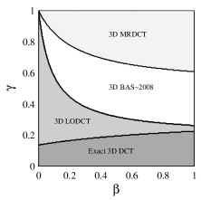
Figure 1: Optimum 3D transformations for different cost function parameters.

Table 3: Coding efficiency and computational complexity percent reduction relative to the exact 3D DCT (considering 3D VR DIF direct algorithm)

	Efficiency		3D Complexity
Method	$C_{g}$	$\eta$	Mult.	Add.	Total
3D SDCT	31.7 %	12.1 %	100 %	17.2 %	33.3 %
3D LODCT	4.9 %	5.6 %	100 %	17.2 %	27.8 %
3D RDCT	7.3 %	7.0 %	100 %	24.1 %	38.9 %
3D MRDCT	16.9 %	13.9 %	100 %	51.7 %	61.1 %
3D BAS-2008	8.0 %	7.6 %	100 %	37.9 %	44.4 %
3D BAS-2009	10.4 %	9.2 %	100 %	37.9 %	50.0 %
3D BAS-2013	10.0 %	9.2 %	100 %	17.2 %	33.3 %
3D IADCT	16.9 %	13.9 %	100 %	51.7 %	61.1 %

4 Interframe Video Coding Based on 3D DCT Approximations

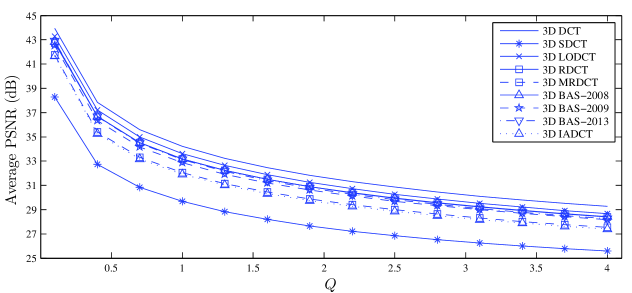
(a) PSNR

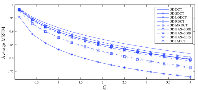
(b) MSSIM

Figure 2: Video compression performance measures.

This section introduces low-complexity interframe video coding schemes [92, 108, 4, 73, 80] equipped with the discussed 3D DCT approximations (cf. Table 1 and (20)). We embed the 3D DCT approximations into a three dimensional block transform coding system based on 3D DCT [92, 108, 4, 73, 80]. We also propose a method to modify a given 3D quantization volume in order to avoid extra computation of such 3D approximate transforms. Then we submit a set of widely employed video sequences to the modified video coding system to evaluate output video quality relative to the original coding scheme.

4.1 Modified Quantization Procedure for Video Compression

In image compression schemes, the quantization step plays a fundamental role since it non-linearly re-scales or discards transform-domain components according to (i) their respective importance to perceived visual quality [12, p. 155] or (ii) data correlational properties [12, p. 156]. In 2D DCT coding, the quantization procedure depends on quantization tables (or matrices) [101, 12] prescribed by adopted standards, such as MPEG [113, 62], H.261 [63] H.263 [64], H.264 [111], and HEVC [65].

As detailed in [22, 112, 83, 78], the diagonal matrix of the approximate DCT (cf. (16)) can be merged into the quantization tables, eliminating the need for additional computation implied by the diagonal elements. However, for the 3D DCT based coding, such tables are not adequate because they are 2D arrays in nature [77, 24, 19, 20]. Instead of a quantization table, a quantization volume is required. In [77, 24, 19], methods to generate 3D quantization volumes are proposed. In this section, we aim at proposing a method for embedding the diagonal matrices described in (20) into a given quantization volume.

Let $\mathcal{Q}\in\mathbb{F}^{N\times N\times N}$ be a previously designed 3D quantization volume, whose entries are given by $q[k_{1},k_{2},k_{3}]$, for $k_{1},k_{2},k_{3}=0,1,\ldots,N-1$. The quantization step performs the following computation [77, 24]:

$$\begin{split}\tilde{y}[k_{1},k_{2},k_{3}]=\operatorname{round}\left(\frac{y[k_{1},k_{2},k_{3}]}{q[k_{1},k_{2},k_{3}]}\right),\\ k_{1},k_{2},k_{3}=0,1,\ldots,N-1,\end{split}$$ (30)

where $y[k_{1},k_{2},k_{3}]$ are transform-domain coefficients according to (20) and $\tilde{y}[k_{1},k_{2},k_{3}]$ are the transform-domain quantized coefficients. The dequantization process is defined by $\hat{y}[k_{1},k_{2},k_{3}]=\tilde{y}[k_{1},k_{2},k_{3}]\cdot q[k_{1},k_{2},k_{3}]$, where $\hat{y}[k_{1},k_{2},k_{3}]$ is an estimative of ${y}[k_{1},k_{2},k_{3}]$ [12].

Now, we split the computation of (20) into two steps: (i) the $i$-mode products involving the low-complexity matrix $\mathbf{T}$, given by:

$$\mathcal{A}=\mathcal{T}\times_{1}\mathbf{T}_{N}\times_{2}\mathbf{T}_{N}\times_{3}\mathbf{T}_{N},$$ (31)

and (ii) the $i$-mode products requiring the diagonal matrix $\mathbf{S}_{N}$. In the Appendix, we demonstrate the following expression:

$$\begin{split}y[k_{1},k_{2},k_{3}]&=a[k_{1},k_{2},k_{3}]\cdot d_{k_{1}}\cdot d_{k_{2}}\cdot d_{k_{3}},\end{split}$$ (32)

where $a[k_{1},k_{2},k_{3}]$ are tensor $\mathcal{A}$ entries given in (31) and $d_{k}$ is the $k$th diagonal element of $\mathbf{S}_{N}$. Applying (32) into (30), we obtain:

$$\begin{split}\tilde{y}[k_{1},k_{2},k_{3}]=\operatorname{round}\left(\frac{a[k_{1},k_{2},k_{3}]\cdot d_{k_{1}}\cdot d_{k_{2}}\cdot d_{k_{3}}}{q[k_{1},k_{2},k_{3}]}\right),\\ k_{1},k_{2},k_{3}=0,1,\ldots,N-1.\end{split}$$ (33)

We propose a new quantization volume $\mathcal{Q}^{*}\in\mathbb{F}^{N\times N\times N}$, whose entries are computed by:

$$q^{*}[k_{1},k_{2},k_{3}]\triangleq\frac{q[k_{1},k_{2},k_{3}]}{d_{k_{1}}\cdot d_{k_{2}}\cdot d_{k_{3}}}.$$ (34)

Replacing (34) in (33), we obtain the modified quantization step as follows:

$$\begin{split}\tilde{y}[k_{1},k_{2},k_{3}]=\operatorname{round}\left(\frac{a[k_{1},k_{2},k_{3}]}{q^{*}[k_{1},k_{2},k_{3}]}\right),\\ k_{1},k_{2},k_{3}=0,1,\ldots,N-1.\end{split}$$ (35)

Notice that only the tensor $\mathcal{A}$ is required to be computed. It is employed as the input data to the modified quantization step (35). Because the computation of $\mathcal{A}$ demands only the low-complexity transformation $\mathbf{T}_{N}$ (see (31)), the computational overhead imposed by diagonal matrix is eliminated. The modified dequantization process can be obtained by a similar procedure and it is furnished by: $\hat{y}[k_{1},k_{2},k_{3}]=\tilde{y}[k_{1},k_{2},k_{3}]\cdot q^{\star}[k_{1},k_{2},k_{3}]$, where

$$q^{\star}[k_{1},k_{2},k_{3}]\triangleq{q[k_{1},k_{2},k_{3}]}\cdot{d_{k_{1}}\cdot d_{k_{2}}\cdot d_{k_{3}}}.$$ (36)

4.2 Video Compression Simulation

A video compression scheme based on [92, 108, 4, 73, 80] was considered. Nine standard CIF [51] YUV video sequences available at [2] were chosen as third-order tensors of size $N_{1}\times N_{2}\times N_{3}$. The CIF video sequences present $N_{1}=352$ and $N_{2}=288$; and we selected 296 consecutive frames ($N_{3}=296$). Each video tensor was divided into $8\times 8\times 8$ smaller tensors, which were applied to the 3D transformation defined in (20), and then submitted to the quantization stage. The 1D DCT approximations shown in Table 1 were considered to derive the 3D approximate methods. In addition, the exact 3D DCT was also included in the experiments for comparison. The quantization volume suggested in [77] was applied to the modified quantization procedure, as described in Section 4.1. The procedure was simulated at quality factors $Q$ ranging in $Q\in[0.1,4.0]$ [12]. The inverse procedure was applied to reconstruct the video sequence. The decoding process includes a modified dequantization and calls to the inverse approximate 3D transformation.

To evaluate the data compression performance, we employed the peak signal to noise ratio (PSNR) [14] and the structural similarity index (SSIM) [117] as figures of merit. The PSNR measure is related to the mean squared error (MSE) according to:

$$\operatorname{PSNR}\triangleq 10\cdot\log_{10}\left(\frac{255^{2}}{\operatorname{MSE}}\right).$$ (37)

Let $t[n_{1},n_{2},n_{3}]$ be the entries of original video tensor $\mathcal{T}$ and $\hat{t}[n_{1},n_{2},n_{3}]$ be the entries of the recovered video tensor $\hat{\mathcal{T}}$. The MSE of the 3D data is computed by [24]:

$$\begin{split}\operatorname{MSE}\triangleq\frac{1}{N_{1}N_{2}N_{3}}\cdot\sum_{n_{1}=0}^{N_{1}-1}\sum_{n_{2}=0}^{N_{2}-1}\sum_{n_{3}=0}^{N_{3}-1}e^{2}[n_{1},n_{2},n_{3}],\end{split}$$ (38)

where $e[n_{1},n_{2},n_{3}]=t[n_{1},n_{2},n_{3}]-\hat{t}[n_{1},n_{2},n_{3}]$. Since SSIM is defined for still images [117], we computed the SSIM between each original frame and its associate compressed frame. Then, the mean SSIM (MSSIM) taken across frames was evaluated, resulting in a performance measure suitable for video sequences.

The average PSNR and average MSSIM for all considered video sequences are shown in Figure 2 at the discussed range of $Q$ values. The 3D DCT effected the highest video quality, whereas the 3D SDCT presented a considerably lower performance when compared to competing approximations. Most approximate methods performed similarly to the exact 3D DCT, specially at low compression rate (small values of $Q$).

In the following analysis, we exclude the 3D SDCT since competing approximations showed considerable higher performance. Generally, the approximate methods presented less than 7% PSNR degradation relative to the exact DCT. For example, for $Q=0.1$, the 3D LODCT shows only $1.53\%$ lower PSNR compared to the exact DCT, whereas the 3D IADCT presents a $5.22\%$ PSNR reduction. For $Q=4$, such values are $2.01\%$ and $6.36\%$, respectively. Figure 3 presents a qualitative comparison for the first frame of the “foreman” video sequence for $Q=0.25$. The frames are essentially indistinguishable. The complete compressed video sequence is available in [39].

(a) Uncompressed

(b) 3D DCT (PSNR=37.8988, MSSIM = 0.9456)

(c) 3D SDCT (PSNR=32.3627, MSSIM = 0.8519)

(d) 3D LODCT (PSNR=37.2166, MSSIM = 0.9393)

(e) 3D RDCT (PSNR=36.7865, MSSIM = 0.9352)

(f) 3D MRDCT (PSNR=36.5764, MSSIM = 0.9280 )

(g) BAS-2008 (PSNR=37.0146, MSSIM = 0.9378)

(h) 3D BAS-2009 (PSNR=36.5367, MSSIM = 0.9341)

(i) 3D BAS-2013 (PSNR=36.3304, MSSIM = 0.9323)

(j) 3D IADCT (PSNR=35.2330, MSSIM = 0.9135)

Figure 3: Qualitative assessment for the first frame of the “foreman” video sequence. The complete compressed video sequence is available in [39].

We assessed the impact of the motion level on the video encoding performance for each discussed methods and for all considered video sequences. As the motion level measure, we adopted the average motion vectors magnitude $\overline{\lvert\mathbf{m}\rvert}$ [44]. The motion vectors were extracted from video frames employing the ARPS motion estimation algorithm [93, 9]. In Table 4, we show the motion level of each considered video sequence.

It is expected that the 3D DCT presents a performance decrease in higher motion level videos since high temporal variation leads to energy dispersion in higher 3D DCT coefficients [82]. However, other factors such as the spatial texture of frames also impacts on the visual quality [44]. Since 3D DCT approximations also aim at preserving the original 3D DCT properties, such behavior is expected to happen in similar fashion. We show in Table 5 the performance of each 3D method at each video sequence, as well as the correlation coefficient $\rho$ between the performance metric and the motion level measure. Indeed, the correlation values show an inverse tendency between performance and motion level, specially for the SSIM metrics, which better captures the perceived visual quality when compared with the PSNR [117]. Furthermore, all approximate methods present similar correlation values to the exact 3D DCT. Therefore, the proposed 3D methods are suitable candidates for replacing the exact 3D DCT in video coding at different motion levels.

Table 4: Motion level of considered video sequences

Sequence index	Sequence	Motion level $\overline{\lvert\mathbf{m}\rvert}$
1	akyio	0.0387
2	container	0.0954
3	news	0.2561
4	silent	0.4877
5	mobile	0.748
6	mother-daughter	0.7594
7	hall-monitor	0.805
8	coastguard	1.7614
9	foreman	2.345

Table 5: Performance of proposed methods for each video sequence and correlation with motion level

Measure	Method	Sequence index									correlation $\rho$
		1	2	3	4	5	6	7	8	9
PSNR (dB)	3D DCT	39.12	35.87	36.33	34.93	26.42	37.74	35.68	30.22	31.69	-0.55
	3D SDCT	34.31	31.41	31.31	30.74	21.05	33.27	32.16	25.77	27.08	-0.51
	3D LODCT	38.27	35.21	35.59	34.42	25.86	37.07	35.24	29.79	31.18	-0.54
	3D RDCT	37.80	34.83	35.06	34.06	25.11	36.66	34.95	29.36	30.82	-0.52
	3D MRDCT	36.71	33.68	33.88	33.13	23.42	35.58	34.28	28.13	29.61	-0.51
	3D BAS-2008	37.88	34.76	35.22	34.12	24.94	36.68	35.06	29.24	30.75	-0.53
	3D BAS-2009	37.52	34.50	34.83	33.87	24.50	36.34	34.81	28.96	30.44	-0.52
	3D BAS-2013	37.69	34.73	35.03	34.10	25.14	36.50	34.90	29.29	30.63	-0.54
	3D IADCT	36.56	33.53	33.76	32.99	23.26	35.41	34.17	28.02	29.51	-0.50
SSIM	3D DCT	0.96	0.93	0.95	0.92	0.87	0.94	0.93	0.86	0.86	-0.84
	3D SDCT	0.92	0.89	0.90	0.84	0.72	0.87	0.89	0.74	0.73	-0.78
	3D LODCT	0.95	0.93	0.94	0.91	0.86	0.93	0.93	0.85	0.84	-0.84
	3D RDCT	0.95	0.92	0.94	0.91	0.84	0.92	0.92	0.84	0.84	-0.82
	3D MRDCT	0.94	0.91	0.93	0.89	0.79	0.91	0.92	0.80	0.80	-0.76
	3D BAS-2008	0.95	0.92	0.94	0.91	0.84	0.93	0.93	0.83	0.84	-0.80
	3D BAS-2009	0.95	0.92	0.94	0.91	0.83	0.92	0.92	0.82	0.83	-0.80
	3D BAS-2013	0.95	0.92	0.94	0.91	0.84	0.92	0.92	0.83	0.83	-0.84
	3D IADCT	0.94	0.91	0.93	0.89	0.78	0.91	0.92	0.79	0.80	-0.76

5 Visual Tracking

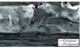
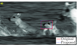
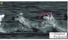
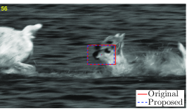
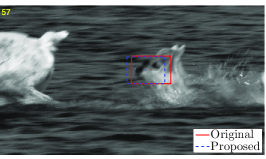
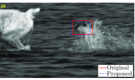
Figure 4: Qualitative tracking results for the “animal” video sequence for representative frames (first, 40th, 43rd, 56th, 57th, and 59th). The full video sequence is available in [40].

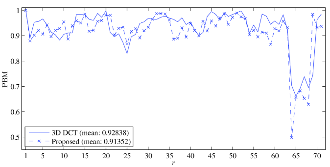
Figure 5: PBM for each $r$th frame of “animal” video sequence.

Visual tracking consists in predicting the location of a target over a frame sequence based on an initial target position. A large variety of tracking methods is available in literature [109]. Immediate applications include: visual surveillance and security control [38, 70, 114], driver assistance and tracking vehicles [38, 7], and wireless sensor visual networks (WSVN) [114, 47]. The class of trackers discussed in [109, 103, 3] employs principal component analysis (PCA) as appearance model [109, 103]. Mathematically, PCA is equivalent to the KLT [53]. Inspired by PCA-based trackers and by the relation between the KLT and the DCT, Li et al. proposed a discriminative learning-based visual tracking method based on the 3D DCT for low-dimensional subspace representation [81]. Such algorithm leads to a computationally more efficient implementation when compared to purely PCA-based techinques [81, 103].

Low-complexity algorithms for visual tracking systems paves the way for real-time computationally demanding applications [26, 7, 124]. As extensively discussed in [83, 112, 22, 57, 78, 34, 10, 14, 15, 17, 97, 33, 36, 41, 35, 59, 102], DCT approximations are emerging tools for DCT-based technologies at a low computational cost. In this section, we embedded a 3D DCT approximation in a video tracking system. We modified the 3D DCT block in [81] in order to compute a 3D DCT approximation, according to (20). The original algorithm in [81] computes $N_{1}\times N_{2}\times N_{3}$ incremental 3D DCT by using a fast Fourier transform (FFT) [5]. Quantities $N_{1}$ and $N_{2}$ were set fixed, whereas $N_{3}$ varied incrementally until a maximum buffer size $T$. The method demands $N_{1}N_{2}\left(\log_{2}N_{1}+\log_{2}N_{2}\right)+N_{1}N_{2}N_{3}\log_{2}N_{3}$ complex multiplications and twice such value of complex additions [81, 13]. We set $N_{1}=N_{2}=T=8$ in order to achieve compatibility with the approximate methods considered in the current work.

Among the DCT approximations shown in Table 1, we selected the MRDCT [10], which possesses the lower additive complexity as shown in Table 2. The IADCT [97] presents the same computational cost, but shows less favorable performance values in 3D video compression simulations. For the transient first frames, where $N_{3}<T$, we employed a combined approximate/exact DCT algorithm using (22) with $R=3$. We utilized the MRDCT matrix for $\hat{\mathbf{C}}_{N_{1}}$ and $\hat{\mathbf{C}}_{N_{2}}$ and exact DCT matrix ${\mathbf{C}}_{N_{3}}$ instead of $\hat{\mathbf{C}}_{N_{3}}$ until $N_{3}$ reaches the final value $N_{3}=T=8$. Then, we computed the 3D MRDCT approximation as proposed in (19) and (20) for all the remaining frames. In this case, the original tracker demands 1920 and 3840 complex multiplications and complex additions, respectively, whereas the modified tracker requires only 2688 real additions, as shown in Table 2. All remaining video tracking parameters were preserved for both original and modified methods.

It is worth mentioning that our main objective is to provide a proof-of-concept for the proposed methods; suggesting low-complexity approximations as a feasible approach for video tracking computation. Consequently, we selected a representative 3D DCT based video tracking system [81] for analysis. Figure 4 shows a qualitative comparison for some representative frames of the “animal” video sequence, from data set available in [1]. Both original and proposed trackers show very close performance. The full video sequence is available in [40].

For a quantitative evaluation, the position-based measure (PBM) [109] was computed. This measure is based on the distance of the tracked bounding box centroid relative to a previously defined ground truth bounding box centroid. The employed ground truth data are provided in [1]. Let $\mathbb{T}_{r}$ and $\mathbb{G}_{r}$ be the tracked and ground truth bounding boxes, respectively, for the $r$th video frame. The PBM is given by [109]:

$$\operatorname{PBM}(r)=1-\frac{\operatorname{D}(r)}{T_{h}(r)},$$ (39)

where $T_{h}(r)=[\operatorname{width}\left(\mathbb{T}_{r}\right)$ $+$ $\operatorname{height}\left(\mathbb{T}_{r}\right)$ $+$ $\operatorname{width}\left(\mathbb{G}_{r}\right)$ $+$ $\operatorname{height}\left(\mathbb{G}_{r}\right)]/2$, and

$$\operatorname{D}(r)=\begin{cases}\parallel\operatorname{cent}\left(\mathbb{T}_{r}\right)-\operatorname{cent}\left(\mathbb{G}_{r}\right)\parallel,&\text{if }\mathbb{G}_{r}\cap\mathbb{T}_{r}\neq\varnothing,\\ T_{h}(r),&\text{otherwise;}\end{cases}$$ (40)

and $\operatorname{cent}(\cdot)$, $\operatorname{width}(\cdot)$, and $\operatorname{height}(\cdot)$ return the centroid, width, and height of the bounding box argument, respectively. The PBM values are confined to the interval $[0,1]$. Value 0 represents a tracking failure and value 1 indicates that the centroid of $\mathbb{T}_{r}$ and $\mathbb{G}_{r}$ are the same. Values close to 1 indicates good tracking performance. Figure 5 shows the PBM for all frames of the “animal” video sequence. The proposed method values tend to follow the original method curve, being sometimes even higher. In average, the proposed method present only $1.6\%$ lower PBM value at a much lower complexity cost, as shown in Table 2 and Table 3.

6 Conclusion

In the current work, an algebraic formulation for linear 3D DCT approximations was proposed in terms of tensor analysis. Several multiplierless 3D DCT approximations were suggested based on state-of-art approximate DCT matrices. The concept was generalized and multidimensional approximate DCT were formulated. Mathematical expressions for the multidimensional complexity cost were derived. Such expressions were considered in the 3D case to assess the computational overhead of the proposed methods.

The approximations were applied for interframe video coding. In such context, we proposed a procedure to modify the quantization volume in order to facilitate the use of low-complexity 3D DCT approximations. The obtained results showed that 3D DCT approximations present competitive performance compared to exact 3D DCT algorithms at a considerably lower computational cost. We also simulated a video tracking system, originally based on the exact 3D DCT, embedded with 3D DCT approximations. Results showed that the modified low-cost method performed very closely to the original method. We conclude that 3D DCT approximations can be effective low-complexity tools for emerging hardware and energy limited 3D DCT-based technologies, and also for current systems that benefit of 3D DCT computation, such as SoftCast broadcasting system [69, 67, 68], 3D quantization-based video encoders [91, 106, 107, 19, 73, 25, 77], transform-based visual trackers [81].

[Proof of Equation (32)]

Let us split (20) into two parts: (i) the $i$-mode products involving only low-complexity matrix $\mathbf{T}_{N}$ and (ii) the $i$-mode products requiring the diagonal matrix $\mathbf{S}_{N}$. Part (i) is given in (31). The next intermediate tensor is

$$\mathcal{B}=\mathcal{A}\times_{1}\mathbf{S}_{N}.$$ (41)

Let the diagonal matrix $\mathbf{S}_{N}$ entries be:

$$s[k,n]\triangleq\begin{cases}d_{k},\quad\text{if }k=n,\\ 0,\quad\text{otherwise},\end{cases}\quad n,k=0,1,\ldots,N-1,$$ (42)

where $d_{k}$ is the $k$th diagonal element of matrix $\mathbf{S}_{N}$. Taking into account (8), tensor $\mathcal{B}$ entries are given by:

$$b[k_{1},n_{2},n_{3}]=\sum_{n_{1}=0}^{N-1}a[n_{1},n_{2},n_{3}]\cdot s[k_{1},n_{1}].$$ (43)

Replacing (42) into (43), we derive:

$$b[k_{1},n_{2},n_{3}]=a[k_{1},n_{2},n_{3}]\cdot d_{k_{1}}.$$ (44)

Now the next intermediate tensor is given by:

$$\mathcal{C}=\mathcal{B}\times_{2}\mathbf{S}_{N}.$$ (45)

In a similar manner, $\mathcal{C}$ entries are furnished by:

$$\begin{split}c[k_{1},k_{2},n_{3}]&=b[k_{1},k_{2},n_{3}]\cdot d_{k_{2}}\\ &=a[k_{1},k_{2},n_{3}]\cdot d_{k_{1}}\cdot d_{k_{2}}.\end{split}$$ (46)

Finally, the tensor $\mathcal{Y}$ given in (20) is also expressed by:

$$\mathcal{Y}=\mathcal{C}\times_{3}\mathbf{S}_{N},$$ (47)

whose entries are analogously obtained by:

$$\begin{split}y[k_{1},k_{2},k_{3}]&=c[k_{1},k_{2},k_{3}]\cdot d_{k_{3}}\\ &=a[k_{1},k_{2},k_{3}]\cdot d_{k_{1}}\cdot d_{k_{2}}\cdot d_{k_{3}}.\end{split}$$ (48)

References

- [1] Computer vision lab. SNU database.
- [2] Xiph.org video test media (2014).
- [3] H. Abdi and L. J. Williams, Principal component analysis, Wiley Interdisciplinary Reviews: Computational Statistics, 2 (2010), pp. 433–459.
- [4] G. P. Abousleman, M. W. Marcellin, and B. R. Hunt, Compression of hyperspectral imagery using the 3-D DCT and hybrid DPCM/DCT, IEEE Transactions on Geoscience and Remote Sensing, 33 (1995), pp. 26–34.
- [5] N. Ahmed, T. Natarajan, and K. R. Rao, Discrete cosine transform, IEEE Transactions on Computers, C-23 (1974), pp. 90–93.
- [6] N. Ahmed and K. R. Rao, Orthogonal Transforms for Digital Signal Processing, Springer, 1975.
- [7] A. Almagambetov, S. Velipasalar, and M. Casares, Robust and computationally lightweight autonomous tracking of vehicle taillights and signal detection by embedded smart cameras, IEEE Transactions on Industrial Electronics, 62 (2015), pp. 3732–3741.
- [8] S. Anitha and B. S. Nagabhushana, Design and development of a novel algorithm for 4D image compression, Digital Image Processing, 3 (2011), pp. 1264–1268.
- [9] A. Barjatya, Block matching algorithms for motion estimation, IEEE Transactions Evolution Computation, 8 (2004), pp. 225–239.
- [10] F. M. Bayer and R. J. Cintra, DCT-like transform for image compression requires 14 additions only, Electronics Letters, 48 (2012), pp. 919–921.
- [11] D. S. Bernstein, Matrix Mathematics: Theory, Facts, and Formulas, Princeton University Press, 2009.
- [12] V. Bhaskaran and K. Konstantinides, Image and Video Compression Standards, Kluwer Academic Publishers, 1997.
- [13] R. E. Blahut, Fast Algorithms for Signal Processing, Cambridge University Press, 2010.
- [14] S. Bouguezel, M. O. Ahmad, and M. N. S. Swamy, Low-complexity 88 transform for image compression, Electronics Letters, 44 (2008), pp. 1249–1250.
- [15] , A fast 88 transform for image compression, in 2009 International Conference on Microelectronics (ICM), 2009, pp. 74–77.
- [16] , A novel transform for image compression, in 53rd IEEE International Midwest Symposium on Circuits and Systems (MWSCAS), 2010, pp. 509–512.
- [17] , Binary discrete cosine and Hartley transforms, IEEE Transactions on Circuits and Systems I: Regular Papers, 60 (2013), pp. 989–1002.
- [18] S. Boussakta, Fast algorithm for the 3-D DCT-II, IEEE Transactions on Signal Processing, 52 (2004), pp. 992–1001.
- [19] N. Bozinović and J. Konrad, Scan order and quantization for 3D-DCT coding, in Proceedings of SPIE Visual Communications and Image Processing, vol. 5150, 2003, p. 1205.
- [20] , Motion analysis in 3D DCT domain and its application to video coding, Signal Processing: Image Communication, 20 (2005), pp. 510–528.
- [21] W. L. Briggs and V. E. Henson, The DFT: an owners’ manual for the discrete Fourier transform, Siam, 1995.
- [22] V. Britanak, P. Yip, and K. R. Rao, Discrete Cosine and Sine Transforms, Academic Press, 2007.
- [23] G. Cardoso and J. Saniie, Performance evaluation of DWT, DCT, and WHT for compression of ultrasonic signals, in IEEE Ultrasonics Symposium, vol. 3, 2004, pp. 2314–2317.
- [24] R. K. W. Chan and M. C. Lee, 3D-DCT quantization as a compression technique for video sequences, Proceedings of the International Conference on Virtual Systems and MultiMedia, (1997), pp. 188–196.
- [25] Y.-L. Chan and W.-C. Siu, Variable temporal-length 3-D discrete cosine transform coding, IEEE Transactions on Image Processing, 6 (1997), pp. 758–763.
- [26] C.-Y. Chang and H. W. Lie, Real-time visual tracking and measurement to control fast dynamics of overhead cranes, IEEE Transactions on Industrial Electronics, 59 (2012), pp. 1640–1649.
- [27] W. H. Chen, C. Smith, and S. Fralick, A fast computational algorithm for the discrete cosine transform, IEEE Transactions on Communications, 25 (1977), pp. 1004–1009.
- [28] X. Chen, Q. Dai, and C. Li, A fast algorithm for computing multidimensional DCT on certain small sizes, IEEE Transactions on Signal Processing, 51 (2003), pp. 213–220.
- [29] Y.-J. Chen, S. Oraintara, and T. Nguyen, Video compression using integer DCT, in Proceedings of International Conference on Image Processing, vol. 2, IEEE, 2000, pp. 844–845.
- [30] Y.-J. Chen, S. Oraintara, T. D. Tran, K. Amaratunga, and T. Q. Nguyen, Multiplierless approximation of transforms using lifting scheme and coordinate descent with adder constraint, in International Conference on Acoustics, Speech, and Signal Processing (ICASSP), vol. 3, IEEE, 2002, pp. III–3136.
- [31] P.-W. Cheng, C.-C. Shen, and P.-C. Li, MPEG compression of ultrasound RF channel data for a real-time software-based imaging system, IEEE Transactions on Ultrasonics, Ferroelectrics, and Frequency Control, 59 (2012), pp. 1413–1420.
- [32] N. Cho, Fast algorithm and implementation of 2-D discrete cosine transform, IEEE Transactions on Circuits and Systems, 38 (1991), pp. 297–305.
- [33] R. J. Cintra, An integer approximation method for discrete sinusoidal transforms, Journal of Circuits, Systems, and Signal Processing, 30 (2011), pp. 1481–1501.
- [34] R. J. Cintra and F. M. Bayer, A DCT approximation for image compression, IEEE Signal Processing Letters, 18 (2011), pp. 579–582.
- [35] R. J. Cintra, F. M. Bayer, V. A. Coutinho, S. Kulasekera, A. Madanayake, and A. Leite, Energy-efficient 8-point DCT approximations: Theory and hardware architectures, Circuits, Systems, and Signal Processing, (2015), pp. 1–21.
- [36] R. J. Cintra, F. M. Bayer, and C. J. Tablada, Low-complexity 8-point DCT approximations based on integer functions, Signal Processing, 99 (2014), pp. 201–214.
- [37] R. J. Clarke, Relation between the Karhunen-Loève and cosine transforms, IEE Proceedings F Communications, Radar and Signal Processing, 128 (1981), pp. 359–360.
- [38] B. Coifman, D. Beymer, P. McLauchlan, and J. Malik, A real-time computer vision system for vehicle tracking and traffic surveillance, Transportation Research Part C: Emerging Technologies, 6 (1998), pp. 271–288.
- [39] V. A. Coutinho, R. J. Cintra, and F. M. Bayer, 3D DCT compressed ‘foreman’ video sequence, July 2016.
- [40] , Approximate tracking: ‘animal’ video sequence, July 2016.
- [41] V. A. Coutinho, R. J. Cintra, F. M. Bayer, S. Kulasekera, and A. Madanayake, A multiplierless pruned DCT-like transformation for image and video compression that requires ten additions only, Journal of Real-Time Image Processing, (2015), pp. 1–9.
- [42] Q. Dai, X. Chen, and C. Lin, Fast algorithms for multidimensional DCT-to-DCT computation between a block and its associated subblocks, IEEE Transactions on Signal Processing, 53 (2005), pp. 3219–3225.
- [43] M. Danciu, M. Gordan, C. Florea, and A. Vlaicu, 3D DCT supervised segmentation applied on liver volumes, in 35th International Conference on Telecommunications and Signal Processing (TSP), IEEE, 2012, pp. 779–783.
- [44] A. M. Dawood and M. Ghanbari, Content-based MPEG video traffic modeling, IEEE Transactions on Multimedia, 1 (1999), pp. 77–87.
- [45] L. De Lathauwer and B. De Moor, From matrix to tensor: Multilinear algebra and signal processing, in Institute of Mathematics and Its Applications Conference Series, vol. 67, Citeseer, 1998, pp. 1–16.
- [46] L. De Lathauwer, B. De Moor, and J. Vandewalle, On the best rank-1 and rank-(r 1, r 2,…, rn) approximation of higher-order tensors, SIAM Journal on Matrix Analysis and Applications, 21 (2000), pp. 1324–1342.
- [47] O. Demigha, W.-K. Hidouci, and T. Ahmed, On energy efficiency in collaborative target tracking in wireless sensor network: a review, IEEE Communications Surveys & Tutorials, 15 (2013), pp. 1210–1222.
- [48] C. Desmouliers, E. Oruklu, and J. Saniie, Adaptive 3D ultrasonic data compression using distributed processing engines, in IEEE International Ultrasonics Symposium (IUS), 2009, pp. 694–697.
- [49] M. Ehrgott, Multicriteria optimization. vol. 491 of lecture notes in economics and mathematical systems, 2005.
- [50] E. Feig and S. Winograd, Fast algorithms for the discrete cosine transform, IEEE Transactions on Signal Processing, 40 (1992), pp. 2174–2193.
- [51] F. H. Fitzek and M. Reisslein, MPEG-4 and H.263 video traces for network performance evaluation, IEEE Network, 15 (2001), pp. 40–54.
- [52] C.-K. Fong and W.-K. Cham, LLM integer cosine transform and its fast algorithm, IEEE Transactions on Circuits and Systems for Video Technology, 22 (2012), pp. 844–854.
- [53] J. J. Gerbrands, On the relationships between SVD, KLT and PCA, Pattern Recognition, 14 (1981), pp. 375–381.
- [54] R. C. Gonzalez and R. Woods, Digital Image Processing, Prentice Hall, 2001.
- [55] S. J. Gortler, R. Grzeszczuk, R. Szeliski, and M. F. Cohen, The lumigraph, in Proceedings of the 23rd annual conference on Computer graphics and interactive techniques, ACM, 1996, pp. 43–54.
- [56] P. Govindan, B. Wang, P. Ravi, and J. Saniie, Hardware and software architectures for computationally efficient three-dimensional ultrasonic data compression, IET Circuits, Devices & Systems, 10 (2016), pp. 54–61.
- [57] T. I. Haweel, A new square wave transform based on the DCT, Signal Processing, 82 (2001), pp. 2309–2319.
- [58] M. T. Heideman, Multiplicative Complexity, Convolution, and the DFT, Signal Processing and Digital Filtering, Springer-Verlag, 1988.
- [59] L. Hnativ, Integer cosine transforms: Methods to construct new order 8, 16 fast transforms and their application, Cybernetics and Systems Analysis, 50 (2014), pp. 913–929.
- [60] R. A. Horn and C. R. Johnson, Matrix analysis, Cambridge university press, 2012.
- [61] H. S. Hou, A fast recursive algorithm for computing the discrete cosine transform, IEEE Transactions on Acoustic, Signal, and Speech Processing, 6 (1987), pp. 1455–1461.
- [62] International Organisation for Standardisation, Generic coding of moving pictures and associated audio information – Part 2: Video, ISO/IEC JTC1/SC29/WG11 - coding of moving pictures and audio, ISO, 1994.
- [63] International Telecommunication Union, ITU-T recommendation H.261 version 1: Video codec for audiovisual services at kbits, tech. rep., ITU-T, 1990.
- [64] , ITU-T recommendation H.263 version 1: Video coding for low bit rate communication, tech. rep., ITU-T, 1995.
- [65] , High efficiency video coding: Recommendation ITU-T H.265, tech. rep., ITU-T Series H: Audiovisual and Multimedia Systems, 2013.
- [66] J. A. Jacob and N. S. Kumar, FPGA implementation of optimal 3D-integer DCT structure for video compression, The Scientific World Journal, 2015 (2015).
- [67] S. Jakubczak and D. Katabi, Softcast: Clean-slate scalable wireless video, in 48th Annual Allerton Conference on Communication, Control, and Computing (Allerton), 2010, pp. 530–533.
- [68] , Softcast: one-size-fits-all wireless video, ACM SIGCOMM Computer Communication Review, 41 (2011), pp. 449–450.
- [69] S. Jakubczak, H. Rahul, and D. Katabi, SoftCast: one-size-fits-all wireless video, ACM SIGCOMM Computer Communication Review, 40 (2010), pp. 449–450.
- [70] O. Javed and M. Shah, Tracking and object classification for automated surveillance, in Computer Vision–ECCV 2002, Springer, 2002, pp. 343–357.
- [71] C. W. Kok, Fast algorithm for computing discrete cosine transform, IEEE Transactions on Signal Processing, 45 (1997), pp. 757 – 760.
- [72] N. Kouadria, N. Doghmane, D. Messadeg, and S. Harize, Low complexity DCT for image compression in wireless visual sensor networks, Electronics Letters, 49 (2013), pp. 1531–1532.
- [73] T. H. Lai and L. Guan, Video coding algorithm using 3-D DCT and vector quantization, in Proceedings of the International Conference on Image Processing, vol. 1, 2002, pp. I–741.
- [74] D. Le Gall, MPEG: A video compression standard for multimedia applications, Communications of the ACM, 34 (1991), pp. 46–58.
- [75] V. Lecuire, L. Makkaoui, and J.-M. Moureaux, Fast zonal DCT for energy conservation in wireless image sensor networks, Electronics Letters, 48 (2012), pp. 125–127.
- [76] B. G. Lee, A new algorithm for computing the discrete cosine transform, IEEE Transactions on Acoustics, Speech and Signal Processing, ASSP-32 (1984), pp. 1243–1245.
- [77] M. Lee, R. K. Chan, and D. A. Adjeroh, Quantization of 3D-DCT coefficients and scan order for video compression, Journal of Visual Communication and Image Representation, 8 (1997), pp. 405–422.
- [78] K. Lengwehasatit and A. Ortega, Scalable variable complexity approximate forward DCT, IEEE Transactions on Circuits and Systems for Video Technology, 14 (2004), pp. 1236–1248.
- [79] M. Levoy and P. Hanrahan, Light field rendering, in Proceedings of the 23rd annual conference on Computer graphics and interactive techniques, ACM, 1996, pp. 31–42.
- [80] L. Li and Z. Hou, Multiview video compression with 3D-DCT, in ITI 5th International Conference on Information and Communications Technology, 2007, pp. 59–61.
- [81] X. Li, A. Dick, C. Shen, A. van den Hengel, and H. Wang, Incremental learning of 3D-DCT compact representations for robust visual tracking, IEEE Transactions on Pattern Analysis and Machine Intelligence, 35 (2013), pp. 863–881.
- [82] X. Li, Q. Guo, and X. Lu, Spatiotemporal statistics for video quality assessment, IEEE Transactions on Image Processing, 25 (2016), pp. 3329–3342.
- [83] J. Liang and T. D. Tran, Fast multiplierless approximation of the DCT with the lifting scheme, IEEE Transactions on Signal Processing, 49 (2001), pp. 3032–3044.
- [84] C. Loeffler, A. Ligtenberg, and G. S. Moschytz, Practical fast 1-D DCT algorithms with 11 multiplications, ICASSP International Conference on Acoustics, Speech, and Signal Processing, 2 (1989), pp. 988–991.
- [85] A. Madanayake, R. J. Cintra, V. Dimitrov, F. M. Bayer, K. A. Wahid, S. Kulasekera, A. Edirisuriya, U. Potluri, S. Madishetty, and N. Rajapaksha, Low-power VLSI architectures for DCT/DWT: precision vs approximation for HD video, biomedical, and smart antenna applications, IEEE Circuits and Systems Magazine, 15 (2015), pp. 25–47.
- [86] V. K. Madisetti, The Digital Signal Processing Handbook, CRC Press, 2009.
- [87] M. Magnor and B. Girod, Data compression for light-field rendering, IEEE Transactions on Circuits and Systems for Video Technology, 10 (2000), pp. 338–343.
- [88] L. Makkaoui, V. Lecuire, and J. Moureaux, Fast zonal DCT-based image compression for wireless camera sensor networks, in 2nd International Conference on Image Processing Theory Tools and Applications (IPTA), IEEE, 2010, pp. 126–129.
- [89] H. S. Malvar, A. Hallapuro, M. Karczewicz, and L. Kerofsky, Low-complexity transform and quantization in H. 264/AVC, IEEE Transactions on circuits and systems for video technology, 13 (2003), pp. 598–603.
- [90] K. Mechouek, N. Kouadria, N. Doghmane, and N. Kaddeche, Low complexity DCT approximation for image compression in wireless image sensor networks, Journal of Circuits, Systems and Computers, (2016).
- [91] A. Mulla, J. Baviskar, A. Baviskar, and C. Warty, Image compression scheme based on zig-zag 3D-DCT and LDPC coding, in Advances in Computing, Communications and Informatics (ICACCI, 2014 International Conference on, 2014, pp. 2380–2384.
- [92] T. R. Natarajan and N. Ahmed, On interframe transform coding, IEEE Transactions on Communications, 25 (1977), pp. 1323–1329.
- [93] Y. Nie and K.-K. Ma, Adaptive rood pattern search for fast block-matching motion estimation, IEEE Transactions on Image Processing, 11 (2002), pp. 1442–1449.
- [94] D. G. Northcott, Multilinear algebra, Cambridge University Press, 2008.
- [95] J.-R. Ohm, M. Van Der Schaar, and J. W. Woods, Interframe wavelet coding-motion picture representation for universal scalability, Signal Processing: Image Communication, 19 (2004), pp. 877–908.
- [96] E. Oruklu and J. Saniie, 3E-1 real-time ultrasonic imaging system based on discrete cosine transform for NDE applications, in IEEE Ultrasonics Symposium, IEEE, 2006, pp. 428–431.
- [97] U. S. Potluri, A. Madanayake, R. J. Cintra, F. M. Bayer, S. Kulasekera, and A. Edirisuriya, Improved 8-point approximate DCT for image and video compression requiring only 14 additions, IEEE Transactions on Circuits and Systems I: Regular Papers, PP (2014), pp. 1–14.
- [98] M. T. Pourazad, C. Doutre, M. Azimi, and P. Nasiopoulos, HEVC: The new gold standard for video compression: How does HEVC compare with H.264/AVC?, IEEE Consumer Electronics Magazine, 1 (2012), pp. 36–46.
- [99] K. R. Rao and J. J. Hwang, Techniques and Standards for Image, Video, and Audio Coding, vol. 70, Prentice Hall New Jersey, 1996.
- [100] K. R. Rao and P. Yip, Discrete Cosine Transform: Algorithms, Advantages, Applications, Academic Press, San Diego, CA, 1990.
- [101] , The Transform and Data Compression Handbook, CRC Press LLC, 2001.
- [102] Y. A. Reznik, A. T. Hinds, and N. Rijavec, Low complexity fixed-point approximation of inverse discrete cosine transform, in International Conference on Acoustics, Speech and Signal Processing (ICASSP), vol. 1, IEEE, 2007, pp. I–1109.
- [103] D. A. Ross, J. Lim, R.-S. Lin, and M.-H. Yang, Incremental learning for robust visual tracking, International Journal of Computer Vision, 77 (2008), pp. 125–141.
- [104] A. J. Sang, T. N. Sun, M. S. Chen, H. X. Chen, and L. L. Liu, 6D vector orthogonal transformation and its application in multiview video coding, The Imaging Science Journal, (2013).
- [105] S. Saponara, Real-time and low-power processing of 3D direct/inverse discrete cosine transform for low-complexity video codec, Journal of Real-Time Image Processing, 7 (2012), pp. 43–53.
- [106] S. Saponara, Real-time and low-power processing of 3D direct/inverse discrete cosine transform for low-complexity video codec, Journal of Real-Time Image Processing, 7 (2012), pp. 43–53.
- [107] S. Sawant and D. A. Adjeroh, Balanced multiple description coding for 3D DCT video, IEEE Transactions on Broadcasting, 57 (2011).
- [108] M. Servais and G. de Jager, Video compression using the three dimensional discrete cosine transform (3D-DCT), in Proceedings of the 1997 South African Symposium on Communications and Signal Processing (COMSIG), IEEE, 1997, pp. 27–32.
- [109] A. W. Smeulders, D. M. Chu, R. Cucchiara, S. Calderara, A. Dehghan, and M. Shah, Visual tracking: An experimental survey, IEEE Transactions on Pattern Analysis and Machine Intelligence, 36 (2014), pp. 1442–1468.
- [110] T. Song and H. Li, Local polar DCT features for image description, IEEE Signal Processing Letters, 20 (2013), pp. 59–62.
- [111] J. V. Team, Recommendation H.264 and ISO/IEC 14 496–10 AVC: Draft ITU-T recommendation and final draft international standard of joint video specification, tech. rep., ITU-T, 2003.
- [112] T. D. Tran, The binDCT: Fast multiplierless approximation of the DCT, IEEE Signal Processing Letters, 7 (2000), pp. 141–144.
- [113] G. K. Wallace, The JPEG still picture compression standard, IEEE Transactions on Consumer Electronics, 38 (1992), pp. xviii–xxxiv.
- [114] X. Wang, S. Wang, and D. Bi, Distributed visual-target-surveillance system in wireless sensor networks, IEEE Transactions on Systems, Man, and Cybernetics, Part B: Cybernetics, 39 (2009), pp. 1134–1146.
- [115] Z. Wang, Fast algorithms for the discrete W transform and for the discrete Fourier transform, IEEE Transactions on Acoustics, Speech and Signal Processing, ASSP-32 (1984), pp. 803–816.
- [116] Z. Wang, Pruning the fast discrete cosine transform, IEEE Transactions on Communications, 39 (1991), pp. 640–643.
- [117] Z. Wang, A. C. Bovik, H. R. Sheikh, and E. P. Simoncelli, Image quality assessment: from error visibility to structural similarity, IEEE Transactions on Image Processing, 13 (2004), pp. 600–612.
- [118] D. Xiangwen, C. Hexin, and Z. Zhijie, 4D-MDCT based adaptive prediction and compensation color video coding, in Proceedings of 7th International Conference on Signal Processing, vol. 2, IEEE, 2004, pp. 1131–1134.
- [119] M. Xue, A. Mian, W. Liu, and L. Li, Automatic 4D facial expression recognition using DCT features, in Winter Conference on Applications of Computer Vision, IEEE, 2015, pp. 199–206.
- [120] Y. Yokotani, R. Geiger, G. D. Schuller, S. Oraintara, and K. Rao, Lossless audio coding using the intMDCT and rounding error shaping, IEEE Transactions on Audio, Speech, and Language Processing, 14 (2006), pp. 2201–2211.
- [121] Y. Zeng, G. Bi, and A. R. Leyman, New polynomial transform algorithm for multidimensional DCT, IEEE Transactions on Signal Processing, 48 (2000), pp. 2814–2821.
- [122] , New polynomial transform algorithm for multidimensional DCT, IEEE Transactions on Signal Processing, 48 (2000), pp. 2814–2821.
- [123] C. Zhang and J. Li, Compression of lumigraph with multiple reference frame (MRF) prediction and just-in-time rendering, in Proceedings of Data Compression Conference, IEEE, 2000, pp. 253–262.
- [124] T. Zhou, X. He, K. Xie, K. Fu, J. Zhang, and J. Yang, Robust visual tracking via efficient manifold ranking with low-dimensional compressive features, Pattern Recognition, 48 (2015), pp. 2459–2473.