Multi-Fidelity Active Learning with GFlowNets

Abstract

In the last decades, the capacity to generate large amounts of data in science and engineering applications has been growing steadily. Meanwhile, the progress in machine learning has turned it into a suitable tool to process and utilise the available data. Nonetheless, many relevant scientific and engineering problems present challenges where current machine learning methods cannot yet efficiently leverage the available data and resources. For example, in scientific discovery, we are often faced with the problem of exploring very large, high-dimensional spaces, where querying a high fidelity, black-box objective function is very expensive. Progress in machine learning methods that can efficiently tackle such problems would help accelerate currently crucial areas such as drug and materials discovery. In this paper, we propose the use of GFlowNets for multi-fidelity active learning, where multiple approximations of the black-box function are available at lower fidelity and cost. GFlowNets are recently proposed methods for amortised probabilistic inference that have proven efficient for exploring large, high-dimensional spaces and can hence be practical in the multi-fidelity setting too. Here, we describe our algorithm for multi-fidelity active learning with GFlowNets and evaluate its performance in both well-studied synthetic tasks and practically relevant applications of molecular discovery. Our results show that multi-fidelity active learning with GFlowNets can efficiently leverage the availability of multiple oracles with different costs and fidelities to accelerate scientific discovery and engineering design.

1 Introduction

Figure 1: Graphic summary of our proposed algorithm for multi-fidelity active learning with GFlowNets. Given a set of $M$ multi-fidelity oracles $f_{1},\ldots,f_{M}$ (center left) with costs $\lambda<\ldots<\lambda_{M}$, respectively, we can construct a data set $\mathcal{D}$ (top left) with annotations from the various oracles. We use this data set to fit a multi-fidelity surrogate model (center) of the posterior $p(f_{m}(x)|x,m,\mathcal{D})$, for instance with Gaussian Processes. The surrogate model is used to calculate the values of a multi-fidelity acquisition function—max-value entropy search (MES) in our experiments—and we train GFlowNet with (a transformation of) the acquisition function as reward. GFlowNet (center right) is trained to sample both an object $x$ and the fidelity $m$ proportionally to the reward function. Once GFlowNet is trained, we can sample $N$ tuples $(x,m)$ and select the top $B$ according to the acquisition function (bottom left). Finally, we annotate each new candidate with the corresponding oracle, add them to the data set and repeat the process. The detailed algorithm is provided in Algorithm 1.

The current most pressing challenges for humanity, such as the climate crisis and the threat of pandemics or antibiotic resistance could be tackled, at least in part, with new scientific discoveries. By way of illustration, materials discovery can play an important role in improving the energy efficiency of energy production and storage; and reducing the costs and duration for drug discovery has the potential to more effectively and rapidly mitigate the consequences of new diseases. In recent years, researchers in materials science, biochemistry and other fields have increasingly adopted machine learning as a tool as it holds the promise to drastically accelerate scientific discovery [9, 74, 5, 15].

Although machine learning has already made a positive impact in scientific discovery applications [62, 31], unleashing its full potential will require improving the current algorithms [2]. For example, typical tasks in potentially impactful applications in materials and drug discovery require exploring combinatorially large, high-dimensional spaces [52, 8], where only small, noisy data sets are available, and obtaining new annotations computationally or experimentally is very expensive. Such scenarios present serious challenges even for the most advanced current machine learning methods.

In the search for a useful discovery, we typically define a quantitative proxy for usefulness, which we can view as a black-box function. One promising avenue for improvement is developing methods that more efficiently leverage the availability of multiple approximations of the target black-box function at lower fidelity but much lower cost than the highest fidelity oracle [12, 17]. For example, the most accurate estimation of the properties of materials and molecules is only typically obtained via synthesis and characterisation in a laboratory. However, this is only feasible for a small number of promising candidates. Approximate quantum mechanics simulations of a larger amount of chemical compounds can be performed via Density Functional Theory (DFT) [46, 57]. However, DFT is still computationally too expensive for high-throughput exploration of large search spaces. Thus, large-scale exploration can only be achieved through cheaper but less accurate oracles. Nonetheless, solely relying on low-fidelity approximations is clearly suboptimal. Ideally, such tasks would be best tackled by methods that can efficiently and adaptively distribute the available computational budget between the multiple oracles depending on the already acquired information.

The past decade has seen significant progress in multi-fidelity Bayesian optimisation (BO) [22, 59], including methods that leverage the potential of deep neural networks [41]. Although highly relevant for scientific discovery, standard BO is not perfectly suited for some of the challenges in materials and drug discovery tasks. First and foremost, BO’s ultimate goal is to find the optimum of an expensive black-box function. However, even the highest fidelity oracles in such problems are underspecified with respect to the actual, relevant, downstream applications. Therefore, it is imperative to develop methods that, instead of “simply” finding the optimum, discover a set of diverse, high-scoring candidates.

Recently, generative flow networks (GFlowNets) [6] have demonstrated their capacity to find diverse candidates through discrete probabilistic modelling, with particularly promising results when embedded in an active learning loop [26]. Here, we propose to extend the applicability of GFlowNets for multi-fidelity active learning.

In this paper, we present an algorithm for multi-fidelity active learning with GFlowNets, depicted in Fig. 1. We provide empirical results in two synthetic benchmark tasks and four practically relevant tasks for biological sequence design and molecular modelling. As a main result, we demonstrate that multi-fidelity active learning with GFlowNets discovers diverse, high-scoring samples when multiple oracles with different fidelities and costs are available, with lower computational cost than its single-fidelity counterpart.

2 Related Work

Our work can be framed within the broad field of active learning (AL), a class of machine learning methods whose goal is to learn an efficient data sampling scheme to accelerate training [56]. For the bulk of the literature in AL, the goal is to train an accurate model $h(x)$ of an unknown target function $f(x)$, as in classical supervised learning. However, in certain scientific discovery problems, which is the motivation of our work, a desirable goal is often to discover multiple, diverse candidates $x$ with high values of $f(x)$. The reason is that the ultimate usefulness of a discovery is extremely expensive to quantify and we always rely on more or less accurate approximations. Since we generally have the option to consider more than one candidate solution, it is safer to generate a set of diverse and apparently good solutions, instead of focusing on the single global optimum of the wrong function.

This distinctive goal is closely connected to related research areas such as Bayesian optimisation [22] and active search [23]. Bayesian optimisation (BO) is an approach grounded in Bayesian inference for the problem of optimising a black-box objective function $f(x)$ that is expensive to evaluate. In contrast to the problem we address in this paper, standard BO typically considers continuous domains and works best in relatively low-dimensional spaces [21]. Nonetheless, in recent years, approaches for BO with structured data [16] and high-dimensional domains [24] have been proposed in the literature. The main difference between BO and the problem we tackle in this paper is that we are interested in finding multiple, diverse samples with high value of $f$ and not only the optimum.

This goal, as well as the discrete nature of the search space, is shared with active search, a variant of active learning in which the task is to efficiently find multiple samples of a valuable (binary) class from a discrete domain $\mathcal{X}$ [23]. This objective was already considered in the early 2000s by Warmuth et al. for drug discovery [66], and more formally analysed in later work [30, 29]. A recent branch of research in stochastic optimisation that considers diversity is so-called Quality-Diversity [11], which typically uses evolutionary algorithms that perform search in the latent space. All these and other problems such as multi-armed bandits [54] and the general framework of experimental design [10] all share the objective of optimising or exploring an expensive black-box function. Formal connections between some of these areas have been established in the literature [60, 20, 27, 18].

Multi-fidelity methods have been proposed in most of these related areas of research. An early survey on multi-fidelity methods for Bayesian optimisation was compiled by Peherstorfer et al. [48], and research on the subject has continued since [50, 59], with the proposal of specific acquisition functions [63] and the use of deep neural networks to improve the modelling [41]. Interestingly, the literature on multi-fidelity active learning [40] is scarcer than on Bayesian optimisation. Recently, works on multi-fidelity active search have also appeared in the literature [45]. Finally, multi-fidelity methods have recently started to be applied in scientific discovery problems [12, 17]. However, the literature is still scarce probably because most approaches do not tackle the specific needs in scientific discovery, such as the need for diverse samples. Here, we aim addressing this need with the use of GFlowNets [6, 28] for multi-fidelity active learning.

3 Method

In this section, we first briefly introduce the necessary background on GFlowNets and active learning. Then, we describe the proposed algorithm for multi-fidelity active learning with GFlowNets.

3.1 Background

GFlowNets

Generative Flow Networks [GFlowNets; 6, 7] are amortised samplers designed for sampling from discrete high-dimensional distributions. Given a space of compositional objects $\mathcal{X}$ and a non-negative reward function $R(x)$, GFlowNets are designed to learn a stochastic policy $\pi$ that generates $x\in\mathcal{X}$ with a probability proportional to the reward, that is $\pi(x)\propto R(x)$. This distinctive property induces sampling diverse, high-reward objects, which is a desirable property for scientific discovery, among other applications [27].

The objects $x\in\mathcal{X}$ are constructed sequentially by sampling transitions $s_{t}{\rightarrow}s_{t+1}\in\mathbb{A}$ between partially constructed objects (states) $s\in\mathcal{S}$, which includes a unique empty state $s_{0}$. The stochastic forward policy is typically parameterised by a neural network $P_{F}(s_{t+1}|s_{t};\theta)$, where $\theta$ denotes the learnable parameters, which models the distribution over transitions $s_{t}{\rightarrow}s_{t+1}$ from the current state $s_{t}$ to the next state $s_{t+1}$. The backward transitions are parameterised too and denoted $P_{B}(s_{t}|s_{t+1};\theta)$. The probability $\pi(x)$ of generating an object $x$ is given by $P_{F}$ and its sequential application:

$$\pi(x)=\sum_{\tau:s_{|\tau|-1}\rightarrow x\in\tau}\prod_{t=0}^{|\tau|-1}P_{F}(s_{t+1}|s_{t};\theta),$$

which sums over all trajectories $\tau$ with terminating state $x$, where $\tau=(s_{0}\rightarrow s_{1}\ldots\rightarrow s_{|\tau|})$ is a complete trajectory. To learn the parameters $\theta$ such that $\pi(x)\propto R(x)$ we use the trajectory balance learning objective [42]

$$\mathcal{L}_{TB}(\tau;\theta)=\left(\log\frac{Z_{\theta}\prod_{t=0}^{n}P_{F}(s_{t+1}|s_{t};\theta)}{R(x)\prod_{t=1}^{n}P_{B}(s_{t}|s_{t+1};\theta)}\right)^{2},$$ (1)

where $Z_{\theta}$ is an approximation of the partition function $\sum_{x\in\mathcal{X}}R(x)$ that is learned. The GFlowNet learning objective supports training from off-policy trajectories, so during training the trajectories are typically sampled from a mixture of the current policy with a uniform random policy. The reward is also tempered to make the policy focus on the modes.

Active Learning

In its simplest formulation, the active learning problem that we consider is as follows: we start with an initial data set $\mathcal{D}=\{(x_{i},f(x_{i}))\}$ of samples $x\in\mathcal{X}$ and their evaluations by an expensive, black-box objective function (oracle) $f:\mathcal{X}\rightarrow\mathbb{R}$, which we use to train a surrogate model $h(x)$. A GFlowNet can then be trained to learn a generative policy $\pi_{\theta}(x)$ using $h(x)$ as reward function, that is $R(x)=h(x)$. Optionally, we can instead train a probabilistic surrogate $p(f|\mathcal{D})$ and use as reward the output of an acquisition function $\alpha(x,p(f|\mathcal{D}))$ that considers the epistemic uncertainty of the surrogate model, as typically done in Bayesian optimisation. Finally, we use the policy $\pi(x)$ to generate a batch of samples to be evaluated by the oracle $f$, we add them to our data set and repeat the process a number of active learning rounds.

While much of the active learning literature [56] has focused on so-called pool-based active learning, where the learner selects samples from a pool of unlabelled data, we here consider the scenario of de novo query synthesis, where samples are selected from the entire object space $\mathcal{X}$. This scenario is particularly suited for scientific discovery [34, 69, 71, 38]. The ultimate goal pursued in active learning applications is also heterogeneous. Often, the goal is the same as in classical supervised machine learning: to train an accurate (surrogate) model $h(x)$ of the unknown target function $f(x)$. For some problems in scientific discovery, we are usually not interested in the accuracy in the entire input space $\mathcal{X}$, but rather in discovering new, diverse objects with high values of $f$. This is connected to other related problems such as Bayesian optimisation [22], active search [23] or experimental design [10], as reviewed in Section 2.

3.2 Multi-Fidelity Active Learning

We now consider the following active learning problem with multiple oracles of different fidelities. Our ultimate goal is to generate a batch of $K$ samples $x\in\mathcal{X}$ according to the following desiderata:

• The samples obtain a high value when evaluated by the objective function $f:\mathcal{X}\rightarrow\mathbb{R}^{+}$.

• The samples in the batch should be distinct and diverse, that is cover distinct high-valued regions of $f$.

Furthermore, we are constrained by a computational budget $\Lambda$ that limits our capacity to evaluate $f$. While $f$ is extremely expensive to evaluate, we have access to a discrete set of surrogate functions (oracles) $\{f_{m}\}_{1\leq m\leq M}:\mathcal{X}\rightarrow\mathbb{R}^{+}$, where $m$ represents the fidelity index and each oracle has an associated cost $\lambda_{m}$. We assume $f_{M}=f$ because there may be even more accurate oracles for the true usefulness but we do not have access to them, which means that even when measured by $f=f_{M}$, diversity remains an important objective. We also assume, without loss of generality, that the larger $m$, the higher the fidelity and that $\lambda_{1}<\lambda_{2}<\ldots<\lambda_{M}$. This scenario resembles many practically relevant problems in scientific discovery, where the objective function $f_{M}$ is indicative but not a perfect proxy of the true usefulness of objects $x$—hence we want diversity—yet it is extremely expensive to evaluate—hence cheaper, approximate models are used in practice.

In multi-fidelity active learning—as well as in multi-fidelity Bayesian optimisation—the iterative sampling scheme consists of not only selecting the next object $x$ (or batch of objects) to evaluate, but also the level of fidelity $m$, such that the procedure is cost-effective.

Our algorithm, MF-GFN, detailed in Algorithm 1, proceeds as follows: An active learning round $j$ starts with a data set of annotated samples $\mathcal{D}_{j}=\{(x_{i},f_{m}(x_{i}),m_{i})\}_{1\leq m\leq M}$. The data set is used to fit a probabilistic multi-fidelity surrogate model $h(x,m)$ of the posterior $p(f_{m}(x)|x,m,\mathcal{D})$. We use Gaussian Processes [53], as is common in Bayesian optimisation, to model the posterior, such that the model $h$ predicts the conditional Gaussian distribution of $f_{m}(x)$ given $(x,m)$ and the existing data set $\mathcal{D}$. We implement a multi-fidelity GP kernel by combining a Matern kernel evaluated on $x$ with a linear downsampling kernel over $m$ [68]. In the higher dimensional problems, we use Deep Kernel Learning [67] to increase the expressivity of the surrogate models. The candidate $x$ is modelled with the deep kernel while the fidelity $m$ is modelled with the same linear downsampling kernel. The output of the surrogate model is then used to compute the value of a multi-fidelity acquisition function $\alpha(x,m)$. In our experiments, we use the multi-fidelity version [63] of max-value entropy search (MES) [65], which is an information-theoretic acquisition function widely used in Bayesian optimisation. MES aims to maximise the mutual information between the value of the queried $x$ and the maximum value attained by the objective function, $f^{\star}$. The multi-fidelity variant is designed to select the candidate $x$ and the fidelity $m$ that maximise the mutual information between $f_{M}^{\star}$ and the oracle at fidelity $m$, $f_{m}$, weighted by the cost of the oracle:

$$\alpha(x,m)=\frac{1}{\lambda_{m}}I(f_{M}^{\star};f_{m}|\mathcal{D}_{j}).$$ (2)

We provide further details about the acquisition function in Section A.3. A multi-fidelity acquisition function can be regarded as a cost-adjusted utility function. Therefore, in order to carry out a cost-aware search, we seek to sample diverse objects with high value of the acquisition function. In this paper, we propose to use a GFlowNet as a generative model trained for this purpose (see further details below in Section 3.3). An active learning round terminates by generating $N$ objects from the sampler (here the GFlowNet policy $\pi$) and forming a batch with the best $B$ objects, according to $\alpha$. Note that $N\gg B$, since sampling from a GFlowNet is relatively inexpensive. The selected objects are annotated by the corresponding oracles and incorporated into the data set, such that $\mathcal{D}_{j+1}=\mathcal{D}_{j}\cup\{(x_{1},f_{m}(x_{1}),m_{1}),\ldots(x_{B},f_{m}(x_{B}),m_{B})\}$.

Input: $\{(f_{m},\lambda_{m})\}$: $M$ oracles and their corresponding costs;

$\mathcal{D}_{0}=\{(x_{i},f_{m}(x_{i}),m_{i})\}$: Initial data set;

$h(x,m)$: Multi-fidelity Gaussian Process surrogate model;

$\alpha(x,m)$: Multi-fidelity acquisition function;

$R(\alpha(x,m),\beta)$: reward function to train the GFlowNet;

$B$: Batch size of oracles queries;

$\Lambda$: Maximum available budget;

$K$: Number of top-scoring candidates to be evaluated at termination;

Result: Top-$K(\mathcal{D})$, Diversity

Initialization: $\Lambda_{j}=0$, $\mathcal{D}=\mathcal{D}_{0}$

while $\Lambda_{j}<\Lambda$ do

       $\bullet$ Fit $h$ on data set $\mathcal{D}$;

       $\bullet$ Train GFlowNet with reward $R(\alpha(x,m),\beta)$ to obtain policy $\pi_{\theta}(x)$;

       $\bullet$ Sample $B$ tuples $(x_{i},m_{i})\sim\pi_{\theta}$;

       $\bullet$ Evaluate each tuple with the corresponding oracle to form batch $\mathcal{B}=\{(x_{1},f_{m}(x_{1}),m_{1}),\ldots,(x_{B},f_{m}(x_{B}),m_{B})\}$;

       $\bullet$ Update data set $\mathcal{D}=\mathcal{D}\cup\mathcal{B}$;

      

end while

Algorithm 1 MF-GFN: Multi-fidelity active learning with GFlowNets. See Section 4.1 for quality (Top-$K({\cal D})$) and diversity metrics. A graphical summary of this algorithm is shown in Fig. 1.

3.3 Multi-Fidelity GFlowNets

In order to use GFlowNets in the multi-fidelity active learning loop described above, we propose to make the GFlowNet sample the fidelity $m$ for each object $x\in\mathcal{X}$ in addition to $x$ itself. Formally, given a baseline GFlowNet with state and transition spaces $\mathcal{S}$ and $\mathbb{A}$, we augment the state space with a new dimension for the fidelity $\mathcal{M^{\prime}}=\{0,1,2,\ldots,M\}$ (including $m=0$, which corresponds to unset fidelity), such that the augmented, multi-fidelity space is $\mathcal{S_{\mathcal{M^{\prime}}}}=\mathcal{S}\cup\mathcal{M^{\prime}}$. The set of allowed transitions $\mathbb{A}_{M}$ is augmented such that a fidelity $m>0$ of a trajectory must be selected once, and only once, from any intermediate state.

Intuitively, allowing the selection of the fidelity at any step in the trajectory should give flexibility for better generalisation. At the end, finished trajectories are the concatenation of an object $x$ and the fidelity $m$, that is $(x,m)\in\mathcal{X}_{\mathcal{M}}=\mathcal{X}\cup\mathcal{M}$. In summary, the proposed approach enables to jointly learn the policy that samples objects in a potentially very large, high-dimensional space, together with the level of fidelity, that maximise a given multi-fidelity acquisition function as reward.

4 Empirical Evaluation

In this section, we describe the evaluation metrics and experiments performed to assess the validity and performance of our proposed approach of multi-fidelity active learning with GFlowNets. Overall, the purpose of this empirical evaluation is to answer the following questions:

• Question 1: Is our multi-fidelity active learning approach able to find high-scoring, diverse samples at lower cost than active learning with a single oracle?

• Question 2: Does our proposed multi-fidelity GFlowNet, which learns to sample fidelities together with objects $(x,m)$, provide any advantage over sampling only objects $x$?

In Section 4.1 we describe the metrics proposed to evaluate the performance our proposed method, as well as the baselines, which we describe in Section 4.2. In Section 4.3, we present results on synthetic tasks typically used in the multi-fidelity BO and active learning literature. In Section 4.4, we present results on more practically relevant tasks for scientific discovery, such as the design of DNA sequences and anti-microbial peptides.

4.1 Metrics

One core motivation in the conception of GFlowNets, as reported in the original paper [6], was the goal of sampling diverse objects with high-score, according to a reward function.

• Mean score, as per the highest fidelity oracle $f_{M}$, of the top-$K$ samples.

• Mean pairwise similarity within the top-$K$ samples.

Furthermore, since here we are interested in the cost effectiveness of the active learning process, in this section we will evaluate the above metrics as a function of the cost accumulated in querying the multi-fidelity oracles. It is important to note that the multi-fidelity approach is not aimed at achieving better mean top-$K$ scores than a single-fidelity active learning counterpart, but rather the same mean top-$K$ scores with a smaller budget.

4.2 Baselines

In order to evaluate our approach, and to shed light on the questions stated above, we consider the following baselines:

• GFlowNet with highest fidelity (SF-GFN): GFlowNet based active learning approach from [26] with the highest fidelity oracle to establish a benchmark for performance without considering the cost-accuracy trade-offs.

• GFlowNet with random fidelities (Random fid. GFN ): Variant of SF-GFN where the candidates are generated with the GFlowNet but the fidelities are picked randomly and a multi-fidelity acquisition function is used, to investigate the benefit of deciding the fidelity with GFlowNets.

• Random candidates and fidelities (Random): Quasi-random approach where the candidates and fidelities are picked randomly and the top $(x,m)$ pairs scored by the acquisition function are queried.

• Multi-fidelity PPO (MF-PPO): Instantiation of multi-fidelity Bayesian optimisation where the acquisition function is optimised using proximal policy optimisation [PPO 55].

4.3 Synthetic Tasks

As an initial assessment of MF-GFNs, we consider two synthetic functions—Branin and Hartmann—widely used in the single- and multi-fidelity Bayesian optimisation literature [50, 59, 32, 41, 19].

Branin

We consider an active learning problem in a two-dimensional space where the target function $f_{M}$ is the Branin function, as modified in [58] and implemented in botorch [3]. We simulate three levels of fidelity, including the true function. The lower-fidelity oracles, the costs of the oracles (0.01, 0.1, 1.0) as well as the number of points queried in the initial training set were adopted from [41]. We provide further details about the task in Section B.1. In order to consider a discrete design space, we map the domain to a discrete $100\times 100$ grid. We model this grid with a GFlowNet as in [6, 42]: starting from the origin $(0,0)$, for any state $s=(x_{1},x_{2})$, the action space consists of the choice between the exit action or the dimension to increment by $1$, provided the next state is in the limits of the grid. Fig. 2(a) illustrates the results for this task. We observe that MF-GFN is able to reach the minimum of the Branin function with a smaller budget than the single-fidelity counterpart and the baselines.

Hartmann

Next, we consider the 6-dimensional Hartmann function as objective $f_{M}$ on a hyper-grid domain. As with Branin, we consider three oracles, adopting the lower-fidelity oracles and the set of costs (0.125, 0.25, 1.0) from [59]. We discretize the domain into a six-dimensional hyper-grid of length 10, yielding $10^{6}$ possible candidate points. The results for the task are illustrated in Fig. 2(b), which indicate that multi-fidelity active learning with GFlowNets (MF-GFN) offers an advantage over single-fidelity active learning (SF-GFN) as well as some of the other baselines in this higher-dimensional synthetic problem as well. Note that while MF-PPO performs better in this task, as shown in the next experiments, MF-PPO tends to collapse to single modes of the function in more complex high-dimensional scenarios.

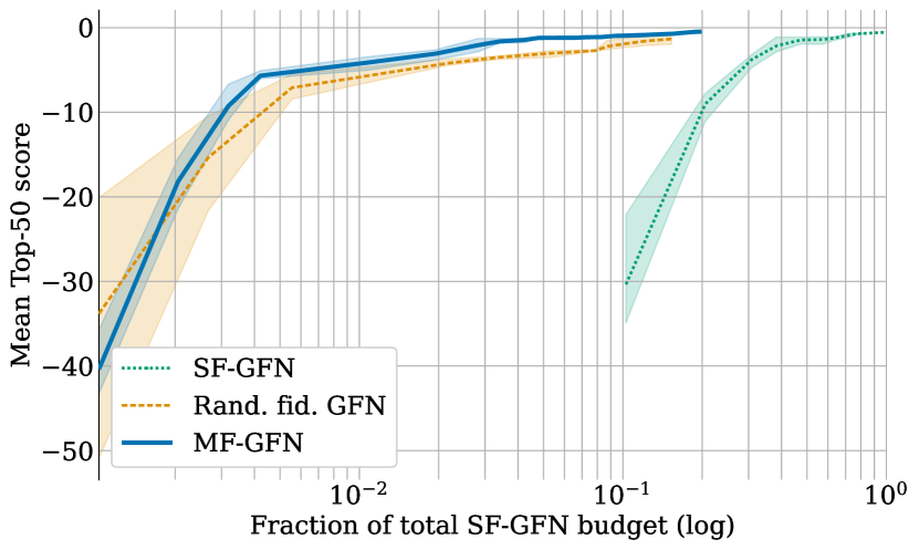
(a) Branin task

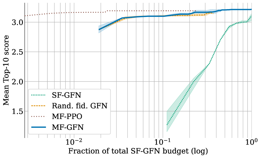
(b) Hartmann task

Figure 2: Results on the synthetic tasks—Branin and Hartmann functions. The curves indicate the mean score $f_{M}$ within the top-50 and top-10 samples (for Branin and Hartmann, respectively) computed at the end of each active learning round and plotted as a function of the budget used. The random baseline is omitted from this plot to facilitate the visualisation since the results were significantly worse in these tasks. We observe that MF-GFN clearly outperforms the single-fidelity counterpart (SF-GFN) and slightly improves upon the GFlowNet baseline that samples random fidelities. On Hartmann, MF-PPO initially outperforms the other methods.

4.4 Benchmark Tasks

While the synthetic tasks are insightful and convenient for analysis, to obtain a more solid assessment of the performance of MF-GFN, we evaluate it, together with the other baselines, on more complex, structured design spaces of practical relevance. We present results on a variety of tasks including DNA aptamers (Section 4.4.1), anti-microbial peptides (Section 4.4.2) and small molecules (Section 4.4.3).

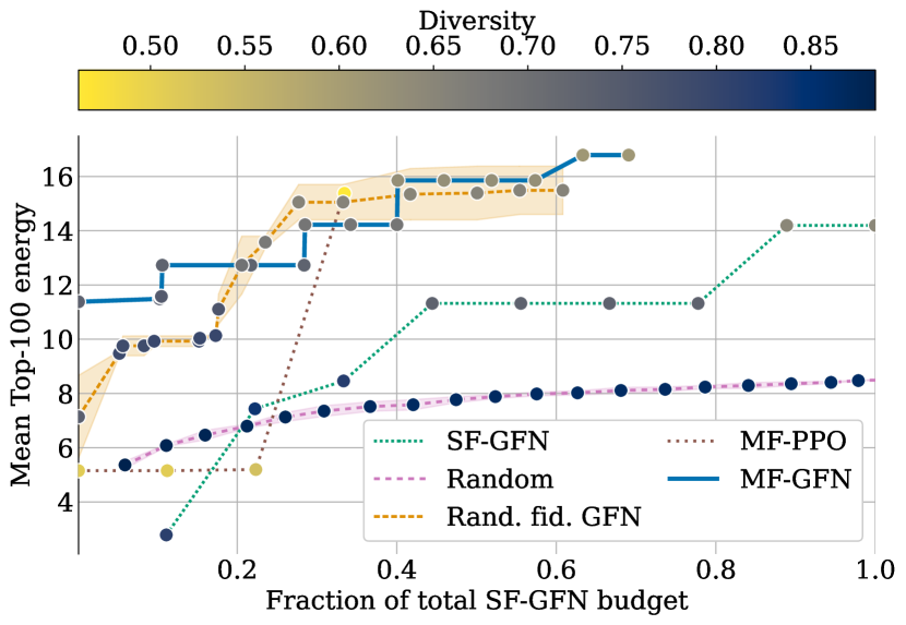
(a) DNA aptamers task

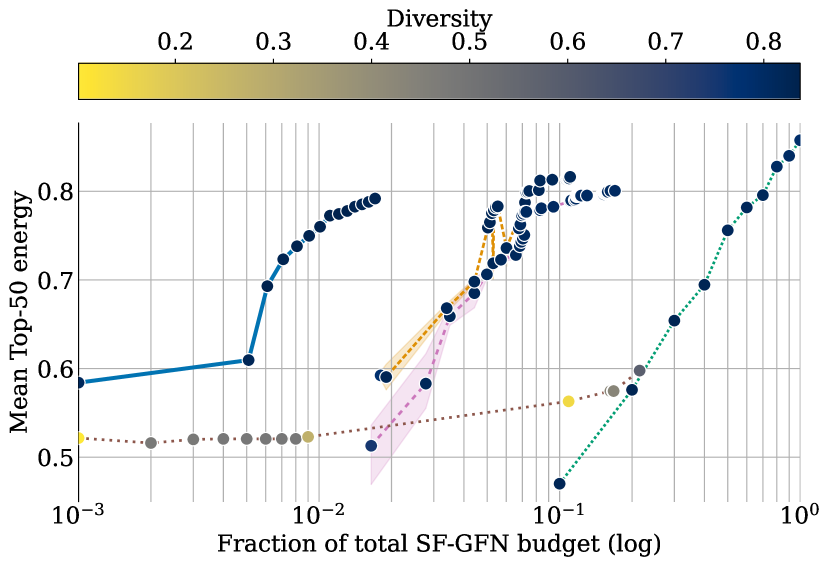
(b) Anti-microbial peptides (AMP) task

Figure 3: Results on the DNA aptamers and AMP tasks. The curves indicate the mean score $f_{M}$ within the top-100 and top-50 samples (for DNA and AMP, respectively) computed at the end of each active learning round and plotted as a function of the budget used. The colour of the markers indicates the diversity within the batch (darker colour of the circular markers indicating more diversity), computed as the average sequence identity (see Appendix C). In both the DNA and AMP tasks, MF-GFN outperforms all baselines in terms of cost efficiency, while obtaining great diversity in the final batch of top-$K$ candidates.

4.4.1 DNA Aptamers

DNA aptamers are single-stranded nucleotide sequences with multiple applications in polymer design due to their specificity and affinity as sensors in crowded biochemical environments [73, 14, 70, 33]. DNA sequences are represented as strings of nucleobases A, C, T or G. In our experiments, we consider fixed-length sequences of 30 bases and design a GFlowNet environment where the action space $\mathbb{A}$ consists of the choice of base to append to the sequence, starting from an empty sequence. This yields a design space of size $|\mathcal{X}|=4^{30}$ (ignoring the selection of fidelity in MF-GFN). As the optimisation objective $f_{M}$ (highest fidelity) we used the free energy of the secondary structure as calculated by NUPACK [72]. As a lower fidelity oracle, we trained a transformer model on 1 million randomly sampled sequences annotated with $f_{M}$, and assigned it a cost $100\times$ smaller than the highest-fidelity oracle. Further details about the task are discussed in Section B.3.

The main results on the DNA aptamers task are presented in Fig. 3(a). We observe that on this task MF-GFN outperforms all other baselines in terms cost efficiency. For instance, MF-GFN achieves the best mean top-$K$ energy achieved by its single-fidelity counterpart with just about $20~{}\%$ of the budget. It is also more efficient than GFlowNet with random fidelities and MF-PPO. Crucially, we also see that MF-GFN maintains a high level of diversity, even after converging to topK reward. On the contrary, MF-PPO is not able to discover diverse samples, as is expected based on prior work [26].

4.4.2 Antimicrobial Peptides

Antimicrobial peptides are short protein sequences which possess antimicrobial properties. As proteins, these are sequences of amino-acids—a vocabulary of 20 along with a special stop token. We consider variable-length protein sequences with up to 50 residues. We use data from DBAASP [51] containing antimicrobial activity labels, which is split into two sets – one used for training the oracle and one as the initial data set in the active learning loop, following  [26]. To establish the multi-fidelity setting, we train different models with different capacities and with different subsets of the data. The details about these oracles along with additional details about the task are discussed in Section B.4.

The results in Fig. 3(b) indicate that even in this task MF-GFN outperforms all other baselines in terms of cost-efficiency. It reaches the same maximum mean top-$K$ score as the random baselines with $10\times$ less budget and almost $100\times$ less budget than SF-GFN. In this task, MF-PPO did not achieve comparable results. Crucially, the diversity of the final batch found by MF-GFN stayed high, satisfying this important criterion in the motivation of this method.

4.4.3 Small Molecules

Molecules are clouds of interacting electrons (and nuclei) described by a set of quantum mechanical descriptions, or properties. These properties dictate their chemical behaviours and applications. Numerous approximations of these quantum mechanical properties have been developed with different methods at different fidelities, with the famous example of Jacob’s ladder in density functional theory [49]. To demonstrate the capability of MF-GFlowNet to function in the setting of quantum chemistry, we consider two proof-of-concept tasks in molecular electronic potentials: maximisation of adiabatic electron affinity (EA) and (negative) adiabatic ionisation potential (IP). These electronic potentials dictate the molecular redox chemistry, and are key quantities in organic semiconductors, photoredox catalysis, or organometallic synthesis. We employed three oracles that correlate with experimental results as approximations of the scoring function, by uses of varying levels of geometry optimisation to obtain approximations to the adiabatic geometries, followed by the calculation of IP or EA with semi-empirical quantum chemistry XTB (see Appendix) [44]. These three oracles had costs of 1, 3 and 7 (respectively), proportional to their computational running demands. We designed the GFlowNet state space by using sequences of SELFIES tokens  [36] (maximum of 64) to represent molecules, starting from an empty sequence; every action consists of appending a new token to the sequence.

The realistic configuration and practical relevance of these tasks allow us to draw stronger conclusions about the usefulness of multi-fidelity active learning with GFlowNets in scientific discovery applications. As in the other tasks evaluated, we here also found MF-GFN to achieve better cost efficiency at finding high-score top-$K$ molecules (Fig. 4), especially for ionization potentials (Fig. 4(a)). By clustering the generated molecules, we find that MF-GFN captures as many modes as random generation, far exceeding that of MF-PPO. Indeed, while MF-PPO seems to outperform MF-GFN in the task of electron affinity (Fig. 4(b)), all generated molecules were from a few clusters, which is of much less utility for chemists.

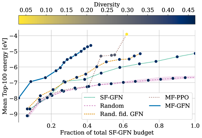
(a) Molecules ionisation potential (IP) task

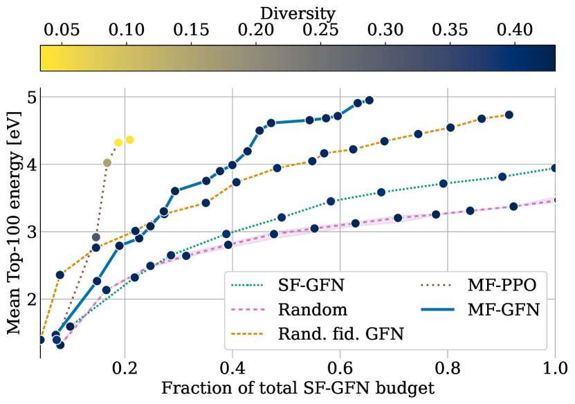
(b) Molecules electron affinity (EA) task

Figure 4: Comparative results on the molecular discovery tasks: (a) ionisation potential (IP), (b) electron affinity (EA). These visualisations are analogous to those in Fig. 3. The diversity of molecules is computed as the average pairwise Tanimoto distance (see Appendix C). Results illustrate the generally faster convergence of MF-GFN to discover a diverse set of molecules with desirable values of the target property.

4.5 Understanding the Impact of Oracle Costs

As discussed in Section 3.2, a multi-fidelity acquisition function like the one we use (defined in Eq. 2) is a cost cost-adjusted utility function. Consequently, the cost of each oracle plays a crucial role in the utility of acquiring each candidate. In our tasks with small molecules (Section 4.4.3), for instance, we used oracles with costs proportional to their computational demands and observed that multi-fidelity active learning largely outperforms single-fidelity active learning. However, depending on the costs of the oracles, the advantage of multi-fidelity methods can diminish significantly.

In order to analyse the impact of the oracle costs on the performance of MF-GFN, we run several experiments on the DNA task (Section 4.4.1), which consists of two oracles, with a variety of oracle costs. In particular, besides the costs used in the experiments presented in Section 4.4.1, with costs $(0.2,20)$ for the lowest and highest fidelity oracles, we run experiments with costs $(1,20)$ and $(10,20)$.

The results, presented in Fig. 5, indeed confirm that the advantage of MF-GFN over SF-GFN decreases as the cost of the lowest-fidelity oracle becomes closer to the cost of the highest-fidelity oracle. However, it is remarkable that even with a ratio of costs as small as $1:2$, MG-GFN still outperforms not only SF-GFN but also MF-PPO in terms of cost effectiveness, without diversity being negatively impacted. It is important to note that in practical scenarios of scientific discovery, the cost of lower fidelity oracles is typically orders of magnitude smaller than the cost of the most accurate oracles, since the latter correspond to wet-lab experiments or expensive computer simulations.

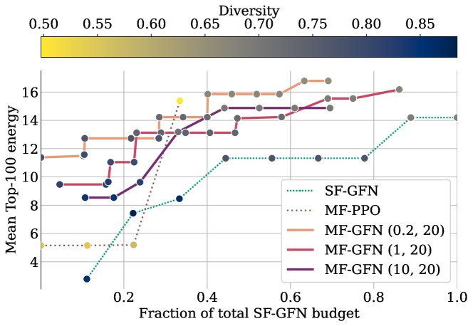
Figure 5: Analysis of the impact of the oracle costs on the performance of MG-GFN on the DNA task. We observe that the advantage over SF-GFN and MF-PPO (0.2, 20) decreases as the cost of the lower fidelity oracle becomes closer to the cost of the highest fidelity oracle. Nonetheless, even with a cost ratio of $1:2$ MF-GFN displays remarkable performance with respect to other methods.

5 Conclusions, Limitations and Future Work

In this paper, we present MF-GFN, the first application of GFlowNets for multi-fidelity active learning. Inspired by the encouraging results of GFlowNets in (single-fidelity) active learning for biological sequence design [26] as a method to discover diverse, high-scoring candidates, we propose MF-GFN to sample the candidates as well as the fidelity at which the candidate is to be evaluated, when multiple oracles are available with different fidelities and costs.

We evaluate the proposed MF-GFN approach in both synthetic tasks commonly used in the multi-fidelity Bayesian optimisation literature and benchmark tasks of practical relevance, such as DNA aptamer generation, antimicrobial peptide design and molecular modelling. Through comparisons with previously proposed methods as well as with variants of our method designed to understand the contributions of different components, we conclude that multi-fidelity active learning with GFlowNets not only outperforms its single-fidelity active learning counterpart in terms of cost effectiveness and diversity of sampled candidates, but it also offers an advantage over other multi-fidelity methods due to its ability to learn a stochastic policy to jointly sample objects and the fidelity of the oracle to be used to evaluate them.

Broader Impact

Our work is motivated by pressing challenges to sustainability and public health, and we envision applications of our approach to drug discovery and materials discovery. However, as with all work on these topics, there is a potential risk of dual use of the technology by nefarious actors [64].

Limitations and Future Work

Aside from the molecular modelling tasks, our empirical evaluations in this paper involved simulated oracles with relatively arbitrary costs. Therefore, future work should evaluate MF-GFN with practical oracles and sets of costs that reflect their computational or financial demands. Furthermore, we believe a promising avenue that we have not explored in this paper is the application of MF-GFN in more complex, structured design spaces, such as hybrid (discrete and continuous) domains [39], as well as multi-fidelity, multi-objective problems [28].

Code availability

The code of the multi-fidelity active learning algorithm presented in this paper is open source and is available on github.com/nikita-0209/mf-al-gfn.

Author contributions

Alex Hernandez-Garcia (AHG) conceived the algorithm, implemented the GFlowNet code and drafted the manuscript. Nikita Saxena (NS) adapted the GFlowNet code to the multi-fidelity setting, implemented the multi-fidelity active learning code and carried out the experiments. The experiments were designed by Moksh Jain (MJ), NS and AHG. Cheng-Hao Liu (CHL) designed the experiments with small molecules and the diversity metrics. Yoshua Bengio (YB) guided the project. All authors contributed to writing the manuscript and analysing the results.

Appendix A Surrogate Models and Acquisition Function

In this appendix, we provide additional details about the surrogate models used in our active learning experiments, as well as about the acquisition function.

A.1 Gaussian Processes

In our multi-fidelity active learning experiments, we model the posterior of $f$ given $x$, $m$ and the current data set $\mathcal{D}_{j}$, assuming that observations are perturbed by noise from a normal distribution $\mathcal{N}(0,\sigma^{2})$. The assumption of normally distributed noise with constant variance is widely used in the BO literature. Consider a set of n points $z_{(1:n)}={(x_{1},m_{1}),(x_{2},m_{2}),\ldots,(x_{n},m_{n})}$ with observed values $y_{(1:n)}={y_{1},y_{2},\ldots,y_{n}}$. We can then use Gaussian Processes such that $f|z_{(1:n)},y_{(1:n)}~{}\sim~{}GP(\mu_{n},K_{n})$ with mean $\mu_{n}$ and covariance function or kernel $K_{n}$ evaluated at point $z=(x,m)$ as

$$\mu_{n}(x)=\mu(x)+K(x,x_{1:n})(K(x_{1:n},x_{1:n})+\sigma^{2}I)^{-1}(y_{1:n}-\mu(x_{1:n}))$$

$$K_{n}(x_{1},x_{2})=K((x_{1},x_{2})-K(x_{1},x_{1:n})(K(x_{1:n},x{1:n})+\sigma^{2}I)^{-1}K(x_{1:n},x_{2}).$$

We adapt the multi-fidelity kernel as proposed in [68], such that the kernel function of the GP is

$$K(z_{1},z_{2})=K_{1}(x_{1},x_{2})\times K_{2}(m_{1},m_{2}),$$

where $K_{1}(\cdot,\cdot)$ is a square-exponential kernel and

$$K_{2}(m_{1},m_{2})=c+(1-m_{1})^{1+\delta}(1-m_{2})^{(1+\delta)},$$

where $c,\delta>0$ are hyper-parameters.

A.2 Deep Kernel Learning

While for the synthetic (simpler) tasks we use exact GPs, for the benchmark tasks we implement deep kernel learning [DKL; 67]. In DKL, the inputs are transformed by

$$k(x_{i},x_{j}|\theta)\rightarrow k(g(x_{i},w),g(x_{j},w)|\theta,w),$$

where the non-linear mapping $g(x,w)$ is a low-dimensional continuous embedding, learnt via a deep neural network—a transformer in our tasks. To scale the GP to large datasets, we implement the stochastic variational GP based on the greedy inducing point method [13]. We adopt the deep kernel learning experimental setup from [61].

A.3 Acquisition Function

Max Value Entropy Search (MES) [65] is an information-theoretic acquisition function. The standard, single-fidelity MES seeks to query the objective function at locations that reduce our current uncertainty in the maximum value of $f^{*}$. It aims to maximise the mutual information between the value of the objective function $f$ when choosing point $x$ and the maximum of the objective function, $f^{\star}$. This contrasts with previously proposed entropy search (ES) criterion, which instead considers the arg max of the objective function. The MES criterion is defined as follows:

$$\alpha=I(f^{\star};y|\mathcal{D}_{j})=H(y|\mathcal{D}_{j})-\mathbb{E}_{f^{\star}}[H(y|\mathcal{D}_{j},f^{\star})|\mathcal{D}_{j}],$$

where $y$ is the outcome of experiment $x$ and $\mathcal{D}_{j}$ is the data set at the $j^{th}$ active learning iteration. and $H(Y)=\mathbb{E}_{Y}[-\log(p(Y))]$ is the differential entropy of random variable $Y$.

The information gain is defined as the reduction in entropy of $y$ provided by knowing the maximal value $f^{\star}$

$$IG(y,m|\mathcal{D}_{n})=H(y|D_{n})-H(y|f^{\star}<m,D_{n})$$

It follows that the MES acquisition function can be expressed in terms of $IG$:

$$\alpha=\mathbb{E}_{m\sim f^{\star}}[IG_{n}(y,m|\mathcal{D}_{n})],$$

where $y\sim\cal{N}(\mu_{A},\sigma_{A})$, $f(x)\sim\cal{N}(\mu_{B},\sigma_{B})$ and the difference between $y$ and $f(x)$ is just independent Gaussian noise.

Replacing the maximisation of an intractable quantity with the maximisation of a lower bound is a well-established strategy. Instead of attempting to evaluate the intractable quantity, $IG$, we evaluate its lower bound $IG^{Approx}$.

Thus, the acquisition function becomes

$$\alpha=\frac{1}{\cal{M}}\sum_{m\in\cal{M}}IG^{Approx}(y,m|\mathcal{D}_{n})$$

$$IG^{Approx}=\frac{1}{2}log|R|-\frac{1}{2\cal{M}}\sum_{m\in\cal{M}}log(1-\rho^{2}\frac{\phi(\gamma(m))}{\Phi(\gamma(m))}[\gamma(m)+\frac{\phi(\gamma(m))}{\Phi(\gamma(m))}]),$$

where $\phi$ and $\Phi$ are the standard normal cumulative distribution and probability density functions (as arising from the expression for the differential entropy of a truncated Gaussian), $\gamma(m)=\frac{m-\mu_{n}(x)}{\sigma_{n}(x)}$ and $R$ is the correlation matrix with elements $R_{i,j}=\frac{\Sigma_{i,j}^{y}}{\Sigma_{i,i}^{y}\Sigma_{j,j}^{y}}$.

This construction is called the General Information-Based Bayesian OptimisatioN (GIBBON) acquisition function [43].

Multi-Fidelity Formulation

Let the maximum of the highest fidelity function $f_{M}$ (when $M$ different fidelities are available to querying) be $f^{\star}_{M}$. We obtain a pair $(x,m)$ which maximally gains information of the optimal value $f^{\star}$ of the highest fidelity per unit cost.

$$\alpha(x,m)=\frac{1}{\lambda_{m}}I(f_{M}^{\star};f_{m}|\mathcal{D}_{j}).$$ (3)

where $\lambda_{m}$ is the cost of the oracle at fidelity $m$.

Appendix B Experimental Details

This appendix presents the details about the experiments presented in the main Section 4. First, we provide general details about all tasks and then present details specific to each task in separate sections.

Policy model architecture

For all tasks, the architecture of the forward policy model to train GFlowNet is multi-layer perceptron with 2 hidden layers and 2048 units per layer. The backward policy model was set to share the parameters with the forward model, except for the parameters of the output layer, which were trained. We use LeakyReLU as our activation function as in [6]. All models are trained with the Adam optimiser [35].

GFlowNet reward

As discussed in Section 3.2, the reward for GFlowNet in our multi-fidelity GFlowNet algorithm is the acquisition function max entropy search (MES) (and its multi-fidelity variant) for all experiments. In order to increase the relative reward of higher values of the acquisition function, we transform the MES value $\alpha$ with the reward function $R(\alpha)=\frac{\alpha\times\rho^{j-1}}{\beta}$, where $j$ is the active learning round.

Budget and initial data set

For each task, we assign a total budget $B=\gamma\times C$, where $C$ is the cost if the highest fidelity oracle. The cost of the lower fidelity oracles are as specified in Section 4. The initial data sets were constructed according to an initial budget. Depending on this initial budget, we set the number of training data points for the single-fidelity baseline, as well as the number of points from each oracle in the multi-fidelity experiments. Task specific information is summarized in Table 2. The initial data set is split into train-validation in the ratio of 9:1 for all tasks.

All the above details for all tasks are summarized in Table 1 and Table 2. Our models are implemented in pytorch [47], and rely on botorch [3] and GPytorch .

Table 1: Implementation details of multi-fidelity experiments of all tasks

Task	Surrogate	$\beta$	$\rho$	$\gamma$
Branin	Exact GP	1	1	300
Hartmann 6D	Exact GP	1e-2	1	100
DNA	DKL	1e-5	2	5120
Antimicrobial Peptides	DKL	1e-5	1	320
Molecules	DKL	1e-6	1.5	1280

Table 2: Oracle costs, initial budget and initial training data sets. Oracles are indexed by increasing level of fidelity.

					Initial training examples
Task	Oracle costs				SF	Multi-Fidelity
	$m=1$	$m=2$	$m=M$	Budget		$m=1$	$m=2$	$m=M$
Branin	0.01	0.1	1	42	4	20	20	2
Hartmann 6D	0.125	0.25	1	200	25	80	40	5
DNA	–	0.2	20	2500	50	2000	2000	10
AMP	0.5	0.5	50	1600	80	–	3000	50
Molecules	1	3	7	1050	150	700	68	16

B.1 Branin

The Branin function is evaluated in the domain $[-5,10]\times[0,15]$ using the following expression:

$$f(x)=(x_{2}-\frac{-1.25x_{1}^{2}}{\pi^{2}}+\frac{5x_{1}}{\pi}-6)^{2}+(10-\frac{5}{4\pi})\cos(x_{1})+10.$$

This corresponds to the modification introduced in [58]. As lower fidelity functions, we used the expressions from [50], which involve non-linear transformations of the true function as well as shifts and non-uniform scalings. The functions, indexed by increasing level of fidelity, are the following:

$$f_{1}(x)=f_{2}(1.2(x+2))-3x_{2}+1$$

$$f_{2}(x)=10\sqrt{f(x-2)}+2(x_{1}-0.5)-3(3x_{2}-1)-1$$

On the discrete set of points obtained after mapping the continuous domain to a $100\times 100$ grid, the explained variance of the oracles are 0.1125, 0.825 and 1, in increasing level of fidelity.

We use the botorch implementation of an exact multi-fidelity Gaussian process as described in A.1 for regression. The active learning batch size $B$ is 30 in the Branin task.

B.2 Hartmann 6D

The true Hartmann function is given by

$$f(x)=\sum_{i=1}^{4}\alpha_{i}exp(-\sum_{j=1}^{3}A_{ij}(x_{j}-P_{ij})^{2}),$$

where $\alpha=[1.0,1.2,3.0,3.2]$ and $A,P\in R^{4\times 6}$ are the following fixed matrices:

$$A=\left[{\begin{array}[]{cccccc}10&3&17&3.5&1.7&8\\ 0.05&10&17&0.1&8&1\\ 3&3.5&1.7&10&17&8\\ 17&8&0.05&10&0.1&1\\ \end{array}}\right]$$

$$P=10^{-4}\times\left[{\begin{array}[]{cccccc}3689&1170&267\\ 4699&4387&7470\\ 1091&8732&5547\\ 381&5743&8828\\ \end{array}}\right]$$

To simulate the lower fidelities, we modify $\alpha$ to $\alpha(m)$ where $\alpha(m)=\alpha+(M-m)\delta$ where $\delta=[0.01,-0.01,-0.1,0.1]$ and $M=3$. The domain is $X=[0,1]^{6}$. This implementation was adopted from [32]. For the surrogate, we use the same exact multi-fidelity GP implementation as of Branin. The active learning batch size is 10.

B.3 DNA

We conduct experiments using a two-oracle setup with costs 20 and 0.2 for the high and low fidelity oracles, respectively. As objective function (highest fidelity oracle) we used the free energy of the secondary structure of DNA sequences obtained via the software NUPACK [72], setting the temperature at 310 K. The free energy can be seen as a proxy of the stability of the sequences. To construct a lower fidelity oracle, we train a transformer with 8 layers, 1024 hidden units per layer and 16 heads. We sampled 1 million random sequences for the training set. The explained variance of the transformer model is 0.8. For the probabilistic surrogate, we implement deep kernel learning. The parameters of the surrogate as well as other details about the DNA task are provided in Table 3.

Table 3: Deep Kernel hyperparameters for the DNA and Antimicrobial tasks

	Hyperparameter	Value
Architecture	Num. of Layers	8
	Num. of Heads	8
	Latent dimension	64
	GP likelihood variance init.	0.25
	GP length scale prior	$\mathcal{N}$(0.7, 0.01)
	Num. of inducing points (SVGP head)	64
Optimisation	Batch Size	128
	Learning Rate	1e-3
	Adam EMA parameters $(\beta 1,\beta 2)$	(0., 1e-2)
	Max. number of Epochs	512
	Early stopping patience (number of epochs)	15
	Early stopping holdout ratio	0.1

B.4 Antimicrobial Peptides

We construct a three-oracle setup where the oracle corresponding to the highest fidelity is trained on data from DBAASP [51]. Each antimicrobial peptide belongs to a group. For the lower fidelity oracles. We divide the data points into two halves such the set of groups present in one half is mutually exclusive of the other. This simulated a setup wherein the lower fidelity oracles specialised only in a specific subregion of the entire sample space. The configurations of the oracle models are present in Table 4. We assigned a cost of 50 to the highest fidelity oracle and 0.5 to both lower fidelity oracles. The explained variance of the oracles was 0.1435, 0.099 and 1 respectively. As for DNA, we implement deep kernel learning with hyperparameters in Table 3.

Table 4: Oracles for the antimicrobial peptides task (indexed by increasing level of fidelity)

Fidelity	# Training points	Model	# Layers	# Hidden units	Epoch
1	3447	MLP	2	512	51
2	3348	MLP	2	512	51
3	6795	MLP	2	1024	101

Table 5: Deep Kernel hyperparameters for the molecular tasks

	Hyperparameter	Value
Architecture	Number of Layers	8
	Number of Heads	8
	Latent dimension	32
	GP likelihood variance init.	0.25
	GP length scale prior	$\mathcal{N}$(0.7, 0.01)
	Number of inducing points (SVGP head)	64
Optimisation	Batch Size	128
	Learning Rate	1e-3
	Adam EMA parameters $(\beta 1,\beta 2)$	(0., 1e-2)
	Max. number of Epochs	512
	Early stopping patience (number of epochs)	15
	Early stopping holdout ratio	0.1

B.5 Small Molecules

We implement the oracles using RDKit 2023.03 [1] and the semi-empirical quantum chemistry package xTB. We use GFN2-xTB [4] method for the single point calculation of ionization potential and electron affinity with empirical correction terms. In the cheapest oracle, we consider one conformer obtained by RDKit with its geometry optimised via force-field (MMFF94[25]), this geometry is used to calculate (vertical) IP/EA. In the second fidelity, we consider two conformers obtained by RDKit, and take the lowest energy conformer after optimisation by MMFF94, and further optimise it via GFN2-xTB to obtain the ground state geometry; this remains a vertical IP/EA calculation. In the highest fidelity oracle, we consider four conformers obtained by RDKit, and take the lowest energy conformer after optimisation by MMFF94, and further optimise it via GFN2-xTB; the corresponding ion is then optimised by GFN2-xTB, and the adiabatic energy difference is obtained via total electronic energy. The fidelities are based on the fact that vertical IP/EA approximates that of adiabatic ones (to varying degrees, depending on the molecule). On a test dataset of 1400 molecules of length<64, the explained variance of the oracles is 0.1359, 0.279, 1 and 0.79, 0.86, 1 for the EA and IP tasks respectively. Further details about the hyperparameters are provided in Table 5.

We note that this is proof-of-concept and hence we do not conduct a full search of conformers, and nor do we use Density Functional Theory calculations, but the highest fidelity oracle has a good correlation with experiments [44].

In the environment for GFN, we consider a set of SELFIES vocabularies containing aliphatic and aromatic carbon, boron, nitrogen, oxygen, fluorine, sulfur, phosphorous, chlorine, and bromine, subject to standard valency rules. We do not consider synthesisability in this study and we note it may negatively impact GFN as unphysical molecules could produce false results for the semi-empirical oracle.

Appendix C Metrics

In this section, we provide additional details about the metrics used for the evaluation of the proposed MF-GFN as well as the baselines.

Mean Top-$K$ Score

We adapt this metric from [6]. At the end of an active learning round, we sample $N$ $(x,m)$ candidates and then select the top-$K$ candidates ($K\ll N$) according to the acquisition function value. In the experiments, we score these top-$K$ candidates with the corresponding oracle. In the figures, we report the mean score according to the highest-fidelity oracle.

Mean Diverse Top-$K$ Score

This is a version of the previous metric by which we restricts the selection of the $K$ candidates to examples that are diverse between each other. We use similarity measures (vide infra) such that we sample the top-$K$ candidates where each candidate it at most similar to each other by a certain threshold. For antimicrobial peptides, the sequence identity threshold is 0.35; for DNA aptamers, the sequence identity threshold is 0.60; for molecules, the Tanimoto similarity distance threshold is 0.35.

Diversity

In order to measure the diversity of a set of candidates, we use the similarity index with the following details for each of the tasks:

• DNA aptamers: The similarity measure is calculated by the mean of pairwise sequence identity between a set of DNA sequences. We utilize global alignment with Needleman-Wunsch algorithm and standard nucleotide substitution matrix, as calculated by biotite package [37].

• Antimicrobial peptides: The similarity measure is calculated by the mean of pairwise sequence identity between a set of peptide sequences. We utilize global alignment with Needleman-Wunsch algorithm and BLOSUM62 substitution matrix, as calculated by biotite package [37].

• Molecules: The similarity measure is calculated by the mean of pairwise Tanimoto distances between a set of molecules. Tanimoto distances are calculated from Morgan Fingerprints (radius of two, size of 2048 bits) as implemented in RDKit package [1].

Appendix D Additional Results

D.1 Energy of Diverse Top-$K$

In this section we complement the results presented in Section 4 with the mean diverse top-$K$ scores, as defined in Appendix C. This metric combines that mean top-$K$ score and the measure of diversity. Figure 6 shows the results on the DNA, AMP and the molecular tasks.

The results with this metric allow us to further confirm that multi-fidelity active learning with GFlowNets is able to discover sets of diverse candidates with high mean scores, as is sought in many scientific discovery applications. In contrast, methods that do not encourage diversity such as RL-based algorithms (MF-PPO) obtain comparatively much lower results with this metric.

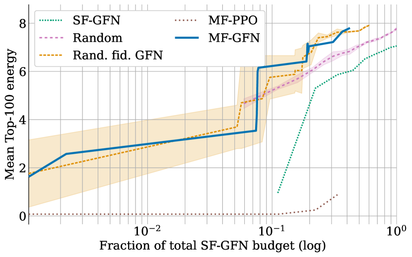
(a) DNA task

(b) Anti-microbial peptides (AMP) task

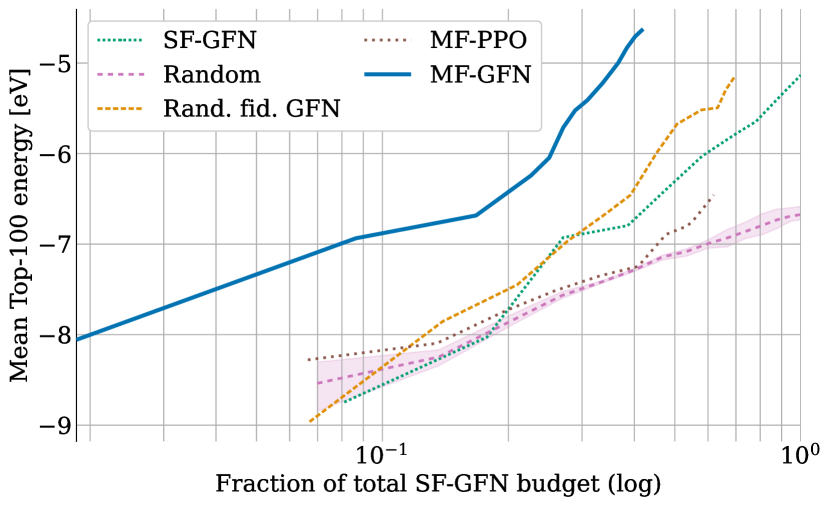
(c) Molecules ionisation potential (IP) task

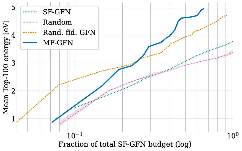
(d) Molecules electron affinity (EA) task

Figure 6: Mean scores (energy) of diverse top-$K$ candidates on the DNA (top left), AMP (top right) and molecular (bottom) tasks. The mean energy is computed across the top-$K$ examples at each active learning round that also satisfy the criteria of diversity. Consistent with the diversity metrics observed in Fig. 3, we here see that GFlowNet-based methods, and especially MF-GFN, obtain good results according to this metric, while MF-PPO achieves comparatively much lower mean energy.

References

- [1] RDKit: Open-source cheminformatics. https://www.rdkit.org.
- [2] Ankit Agrawal and Alok Choudhary. Perspective: Materials informatics and big data: Realization of the “fourth paradigm” of science in materials science. APL Materials, 4(5):053208, 2016.
- [3] Maximilian Balandat, Brian Karrer, Daniel R. Jiang, Samuel Daulton, Benjamin Letham, Andrew Gordon Wilson, and Eytan Bakshy. BoTorch: A Framework for Efficient Monte-Carlo Bayesian Optimization. In Advances in Neural Information Processing Systems (NeurIPS), volume 33, 2020.
- [4] Christoph Bannwarth, Sebastian Ehlert, and Stefan Grimme. GFN2-xTB—an accurate and broadly parametrized self-consistent tight-binding quantum chemical method with multipole electrostatics and density-dependent dispersion contributions. Journal of Chemical Theory and Computation, 15(3):1652–1671, 2019.
- [5] Ali Bashir, Qin Yang, Jinpeng Wang, Stephan Hoyer, Wenchuan Chou, Cory McLean, Geoff Davis, Qiang Gong, Zan Armstrong, Junghoon Jang, et al. Machine learning guided aptamer refinement and discovery. Nature Communications, 12(1):2366, 2021.
- [6] Emmanuel Bengio, Moksh Jain, Maksym Korablyov, Doina Precup, and Yoshua Bengio. Flow network based generative models for non-iterative diverse candidate generation. In Advances in Neural Information Processing Systems (NeurIPS), volume 34, 2021.
- [7] Yoshua Bengio, Salem Lahlou, Tristan Deleu, Edward J. Hu, Mo Tiwari, and Emmanuel Bengio. GFlowNet foundations. arXiv preprint arXiv:2111.09266, 2021.
- [8] Regine S Bohacek, Colin McMartin, and Wayne C Guida. The art and practice of structure-based drug design: a molecular modeling perspective. Medicinal Research Reviews, 16(1):3–50, 1996.
- [9] Keith T Butler, Daniel W Davies, Hugh Cartwright, Olexandr Isayev, and Aron Walsh. Machine learning for molecular and materials science. Nature, 559(7715):547–555, 2018.
- [10] Kathryn Chaloner and Isabella Verdinelli. Bayesian experimental design: A review. Statistical Science, pages 273–304, 1995.
- [11] Konstantinos Chatzilygeroudis, Antoine Cully, Vassilis Vassiliades, and Jean-Baptiste Mouret. Quality-diversity optimization: a novel branch of stochastic optimization. In Black Box Optimization, Machine Learning, and No-Free Lunch Theorems, pages 109–135. Springer, 2021.
- [12] Chi Chen, Yunxing Zuo, Weike Ye, Xiangguo Li, and Shyue Ping Ong. Learning properties of ordered and disordered materials from multi-fidelity data. Nature Computational Science, 1(1):46–53, 2021.
- [13] Laming Chen, Guoxin Zhang, and Hanning Zhou. Fast greedy map inference for determinantal point process to improve recommendation diversity. arXiv preprint arXiv:1709.05135, 2018.
- [14] David R Corey, Masad J Damha, and Muthiah Manoharan. Challenges and opportunities for nucleic acid therapeutics. Nucleic Acid Therapeutics, 32(1):8–13, 2022.
- [15] Payel Das, Tom Sercu, Kahini Wadhawan, Inkit Padhi, Sebastian Gehrmann, Flaviu Cipcigan, Vijil Chenthamarakshan, Hendrik Strobelt, Cicero Dos Santos, Pin-Yu Chen, et al. Accelerated antimicrobial discovery via deep generative models and molecular dynamics simulations. Nature Biomedical Engineering, 5(6):613–623, 2021.
- [16] Aryan Deshwal and Janardhan Rao Doppa. Combining latent space and structured kernels for bayesian optimization over combinatorial spaces. In Advances in Neural Information Processing Systems (NeurIPS), volume 34, 2021.
- [17] Clyde Fare, Peter Fenner, Matthew Benatan, Alessandro Varsi, and Edward O Pyzer-Knapp. A multi-fidelity machine learning approach to high throughput materials screening. npj computational materials, 8(1):257, 2022.
- [18] Francesco Di Fiore, Michela Nardelli, and Laura Mainini. Active learning and Bayesian optimization: a unified perspective to learn with a goal. arXiv preprint arXiv:2303.01560, 2023.
- [19] Jose Pablo Folch, Robert M Lee, Behrang Shafei, David Walz, Calvin Tsay, Mark van der Wilk, and Ruth Misener. Combining multi-fidelity modelling and asynchronous batch Bayesian optimization. Computers & Chemical Engineering, 172:108194, 2023.
- [20] Adam Evan Foster. Variational, Monte Carlo and policy-based approaches to Bayesian experimental design. PhD thesis, University of Oxford, 2021.
- [21] Peter I. Frazier. A tutorial on bayesian optimization. arXiv preprint arXiv:1807.02811, 2018.
- [22] Roman Garnett. Bayesian optimization. Cambridge University Press, 2023.
- [23] Roman Garnett, Yamuna Krishnamurthy, Xuehan Xiong, Jeff Schneider, and Richard Mann. Bayesian optimal active search and surveying. arXiv preprint arXiv:1206.6406, 2012.
- [24] Antoine Grosnit, Rasul Tutunov, Alexandre Max Maraval, Ryan-Rhys Griffiths, Alexander I. Cowen-Rivers, Lin Yang, Lin Zhu, Wenlong Lyu, Zhitang Chen, Jun Wang, Jan Peters, and Haitham Bou-Ammar. High-dimensional Bayesian optimisation with variational autoencoders and deep metric learning. arXiv preprint arXiv:2106.03609, 2021.
- [25] Thomas A Halgren. Merck molecular force field. I. Basis, form, scope, parameterization, and performance of MMFF94. Journal of Computational Chemistry, 17(5-6):490–519, 1996.
- [26] Moksh Jain, Emmanuel Bengio, Alex Hernandez-Garcia, Jarrid Rector-Brooks, Bonaventure FP Dossou, Chanakya Ajit Ekbote, Jie Fu, Tianyu Zhang, Michael Kilgour, Dinghuai Zhang, et al. Biological sequence design with GFlowNets. In International Conference on Machine Learning (ICML), volume 162. PMLR, 2022.
- [27] Moksh Jain, Tristan Deleu, Jason Hartford, Cheng-Hao Liu, Alex Hernandez-Garcia, and Yoshua Bengio. GFlowNets for AI-driven scientific discovery. Digital Discovery, 2023.
- [28] Moksh Jain, Sharath Chandra Raparthy, Alex Hernandez-Garcia, Jarrid Rector-Brooks, Yoshua Bengio, Santiago Miret, and Emmanuel Bengio. Multi-objective GFlowNets. In International Conference on Machine Learning (ICML), 2023.
- [29] Shali Jiang, Roman Garnett, and Benjamin Moseley. Cost effective active search. In Advances in Neural Information Processing Systems (NeurIPS), volume 32, 2019.
- [30] Shali Jiang, Gustavo Malkomes, Geoff Converse, Alyssa Shofner, Benjamin Moseley, and Roman Garnett. Efficient nonmyopic active search. In International Conference on Machine Learning (ICML), volume 70. PMLR, 2017.
- [31] John Jumper, Richard Evans, Alexander Pritzel, Tim Green, Michael Figurnov, Olaf Ronneberger, Kathryn Tunyasuvunakool, Russ Bates, Augustin Žídek, Anna Potapenko, et al. Highly accurate protein structure prediction with AlphaFold. Nature, 596(7873):583–589, 2021.
- [32] Kirthevasan Kandasamy, Gautam Dasarathy, Junier B. Oliva, Jeff Schneider, and Barnabas Poczos. Multi-fidelity gaussian process bandit optimisation. Journal of Artificial Intelligence Research (JAIR), 66:151–196, 2019.
- [33] Michael Kilgour, Tao Liu, Brandon D Walker, Pengyu Ren, and Lena Simine. E2EDNA: Simulation protocol for DNA aptamers with ligands. Journal of Chemical Information and Modeling, 61(9):4139–4144, 2021.
- [34] Ross D King, Kenneth E Whelan, Ffion M Jones, Philip GK Reiser, Christopher H Bryant, Stephen H Muggleton, Douglas B Kell, and Stephen G Oliver. Functional genomic hypothesis generation and experimentation by a robot scientist. Nature, 427(6971):247–252, 2004.
- [35] Diederik P. Kingma and Jimmy Ba. Adam: A method for stochastic optimization. In International Conference on Learning Representations (ICLR), 2015.
- [36] Mario Krenn, Florian Häse, AkshatKumar Nigam, Pascal Friederich, and Alan Aspuru-Guzik. Self-referencing embedded strings (SELFIES): A 100% robust molecular string representation. Machine Learning: Science and Technology, 1(4):045024, 2020.
- [37] Patrick Kunzmann and Kay Hamacher. Biotite: a unifying open source computational biology framework in Python. BMC Bioinformatics, 19:1–8, 2018.
- [38] A Gilad Kusne, Heshan Yu, Changming Wu, Huairuo Zhang, Jason Hattrick-Simpers, Brian DeCost, Suchismita Sarker, Corey Oses, Cormac Toher, Stefano Curtarolo, et al. On-the-fly closed-loop materials discovery via Bayesian active learning. Nature Communications, 11(1):5966, 2020.
- [39] Salem Lahlou, Tristan Deleu, Pablo Lemos, Dinghuai Zhang, Alexandra Volokhova, Alex Hernández-García, Léna Néhale Ezzine, Yoshua Bengio, and Nikolay Malkin. A theory of continuous generative flow networks. In International Conference on Machine Learning (ICML), 2023.
- [40] Shibo Li, Robert M Kirby, and Shandian Zhe. Deep multi-fidelity active learning of high-dimensional outputs. In International Conference on Artificial Intelligence and Statistics (AISTATS), volume 151, pages 1694–1711. PMLR, 2022.
- [41] Shibo Li, Wei Xing, Mike Kirby, and Shandian Zhe. Multi-fidelity bayesian optimization via deep neural networks. In Advances in Neural Information Processing Systems (NeurIPS), volume 33, 2020.
- [42] Nikolay Malkin, Moksh Jain, Emmanuel Bengio, Chen Sun, and Yoshua Bengio. Trajectory balance: Improved credit assignment in GFlowNets. In Advances in Neural Information Processing Systems (NeurIPS), volume 35, 2022.
- [43] Henry B. Moss, David S. Leslie, Javier Gonzalez, and Paul Rayson. GIBBON: General-purpose information-based bayesian optimisation. Journal of Machine Learning Research (JMLR), 22(235):1–49, 2021.
- [44] Hagen Neugebauer, Fabian Bohle, Markus Bursch, Andreas Hansen, and Stefan Grimme. Benchmark study of electrochemical redox potentials calculated with semiempirical and dft methods. The Journal of Physical Chemistry A, 124(35):7166–7176, 2020.
- [45] Quan Nguyen, Arghavan Modiri, and Roman Garnett. Nonmyopic multifidelity active search. In International Conference on Machine Learning (ICML), volume 139. PMLR, 2021.
- [46] Robert G Parr. Density functional theory of atoms and molecules. In Horizons of Quantum Chemistry: Proceedings of the Third International Congress of Quantum Chemistry Held at Kyoto, Japan, October 29-November 3, 1979, pages 5–15. Springer, 1980.
- [47] Adam Paszke, Sam Gross, Francisco Massa, Adam Lerer, James Bradbury, Gregory Chanan, Trevor Killeen, Zeming Lin, Natalia Gimelshein, Luca Antiga, Alban Desmaison, Andreas Köpf, Edward Yang, Zach DeVito, Martin Raison, Alykhan Tejani, Sasank Chilamkurthy, Benoit Steiner, Lu Fang, Junjie Bai, and Soumith Chintala. PyTorch: An imperative style, high-performance deep learning library. In Advances in Neural Information Processing Systems (NeurIPS), volume 32, 2019.
- [48] Benjamin Peherstorfer, Karen Willcox, and Max Gunzburger. Survey of multifidelity methods in uncertainty propagation, inference, and optimization. SIAM Review, 60(3):550–591, 2018.
- [49] John P Perdew and Karla Schmidt. Jacob’s ladder of density functional approximations for the exchange-correlation energy. AIP Conference Proceedings, 577(1):1–20, 2001.
- [50] Paris Perdikaris, M. Raissi, Andreas C. Damianou, ND Lawrence, and George Em Karniadakis. Nonlinear information fusion algorithms for data-efficient multi-fidelity modelling. Proceedings of the Royal Society A: Mathematical, Physical and Engineering Sciences, 473(2198), 2017.
- [51] Malak Pirtskhalava, Anthony A Amstrong, Maia Grigolava, Mindia Chubinidze, Evgenia Alimbarashvili, Boris Vishnepolsky, Andrei Gabrielian, Alex Rosenthal, Darrell E Hurt, and Michael Tartakovsky. DBAASP v3: database of antimicrobial/cytotoxic activity and structure of peptides as a resource for development of new therapeutics. Nucleic Acids Research, 49(D1):D288–D297, 2021.
- [52] Pavel G Polishchuk, Timur I Madzhidov, and Alexandre Varnek. Estimation of the size of drug-like chemical space based on GDB-17 data. Journal of Computer-Aided Molecular Design, 27:675–679, 2013.
- [53] Carl Edward Rasmussen and Christopher K. I. Williams. Gaussian Processes for Machine Learning. The MIT Press, 11 2005.
- [54] Herbert E. Robbins. Some aspects of the sequential design of experiments. Bulletin of the American Mathematical Society, 58:527–535, 1952.
- [55] John Schulman, Filip Wolski, Prafulla Dhariwal, Alec Radford, and Oleg Klimov. Proximal policy optimization algorithms. arXiv preprint arXiv:1707.06347, 2017.
- [56] Burr Settles. Active learning literature survey. Independent Technical Report, 2009.
- [57] David S Sholl and Janice A Steckel. Density functional theory: a practical introduction. John Wiley & Sons, 2022.
- [58] András Sobester, Alexander Forrester, and Andy Keane. Engineering Design via Surrogate Modelling. Appendix: Example Problems, pages 195–203. John Wiley & Sons, Ltd, 2008.
- [59] Jialin Song, Yuxin Chen, and Yisong Yue. A general framework for multi-fidelity Bayesian optimization with Gaussian processes. In International Conference on Artificial Intelligence and Statistics, volume 89. PMLR, 2018.
- [60] Niranjan Srinivas, Andreas Krause, Sham M Kakade, and Matthias Seeger. Gaussian process optimization in the bandit setting: No regret and experimental design. In International Conference on Machine Learning (ICML), 2010.
- [61] Samuel Stanton, Wesley Maddox, Nate Gruver, Phillip Maffettone, Emily Delaney, Peyton Greenside, and Andrew Gordon Wilson. Accelerating Bayesian optimization for biological sequence design with denoising autoencoders. In International Conference on Machine Learning (ICML), volume 162. PMLR, 2022.
- [62] Jonathan M Stokes, Kevin Yang, Kyle Swanson, Wengong Jin, Andres Cubillos-Ruiz, Nina M Donghia, Craig R MacNair, Shawn French, Lindsey A Carfrae, Zohar Bloom-Ackermann, et al. A deep learning approach to antibiotic discovery. Cell, 180(4):688–702, 2020.
- [63] Shion Takeno, Hitoshi Fukuoka, Yuhki Tsukada, Toshiyuki Koyama, Motoki Shiga, Ichiro Takeuchi, and Masayuki Karasuyama. Multi-fidelity Bayesian optimization with max-value entropy search and its parallelization. In International Conference on Machine Learning (ICML), volume 119. PMLR, 2020.
- [64] Fabio Urbina, Filippa Lentzos, Cédric Invernizzi, and Sean Ekins. Dual use of artificial-intelligence-powered drug discovery. Nature Machine Intelligence, 4(3):189–191, 2022.
- [65] Zi Wang and Stefanie Jegelka. Max-value entropy search for efficient Bayesian optimization. In International Conference on Machine Learning (ICML), volume 70. PMLR, 2017.
- [66] Manfred KK Warmuth, Gunnar Rätsch, Michael Mathieson, Jun Liao, and Christian Lemmen. Active learning in the drug discovery process. In Advances in Neural Information Processing Systems (NeurIPS), volume 14, 2001.
- [67] Andrew Gordon Wilson, Zhiting Hu, Ruslan Salakhutdinov, and Eric P Xing. Deep kernel learning. In International Conference on Artificial Intelligence and Statistics (AISTATS), pages 370–378. PMLR, 2016.
- [68] Jian Wu, Saul Toscano-Palmerin, Peter I. Frazier, and Andrew Gordon Wilson. Practical multi-fidelity bayesian optimization for hyperparameter tuning. In Uncertainty in Artificial Intelligence Conference (UAI), volume 115, pages 788–798. PMLR, 2019.
- [69] Dezhen Xue, Prasanna V Balachandran, John Hogden, James Theiler, Deqing Xue, and Turab Lookman. Accelerated search for materials with targeted properties by adaptive design. Nature Communications, 7(1):1–9, 2016.
- [70] Joseph D Yesselman, Daniel Eiler, Erik D Carlson, Michael R Gotrik, Anne E d’Aquino, Alexandra N Ooms, Wipapat Kladwang, Paul D Carlson, Xuesong Shi, David A Costantino, et al. Computational design of three-dimensional RNA structure and function. Nature Nanotechnology, 14(9):866–873, 2019.
- [71] Ruihao Yuan, Zhen Liu, Prasanna V Balachandran, Deqing Xue, Yumei Zhou, Xiangdong Ding, Jun Sun, Dezhen Xue, and Turab Lookman. Accelerated discovery of large electrostrains in BaTiO3-based piezoelectrics using active learning. Advanced Materials, 30(7):1702884, 2018.
- [72] Joseph N Zadeh, Conrad D Steenberg, Justin S Bois, Brian R Wolfe, Marshall B Pierce, Asif R Khan, Robert M Dirks, and Niles A Pierce. NUPACK: Analysis and design of nucleic acid systems. Journal of Computational Chemistry, 32(1):170–173, 2011.
- [73] Wenhu Zhou, Runjhun Saran, and Juewen Liu. Metal sensing by DNA. Chemical Reviews, 117(12):8272–8325, 2017.
- [74] C Lawrence Zitnick, Lowik Chanussot, Abhishek Das, Siddharth Goyal, Javier Heras-Domingo, Caleb Ho, Weihua Hu, Thibaut Lavril, Aini Palizhati, Morgane Riviere, et al. An introduction to electrocatalyst design using machine learning for renewable energy storage. arXiv preprint arXiv:2010.09435, 2020.