A Primal-Dual Data-Driven Method for
Computational Optical Imaging with a Photonic Lantern

Abstract

Optical fibres aim to image in-vivo biological processes. In this context, high spatial resolution and stability to fibre movements are key to enable decision-making processes (e.g., for microendoscopy). Recently, a single-pixel imaging technique based on a multicore fibre photonic lantern has been designed, named computational optical imaging using a lantern (COIL). A proximal algorithm based on a sparsity prior, dubbed SARA-COIL, has been further proposed to enable image reconstructions for high resolution COIL microendoscopy. In this work, we develop a data-driven approach for COIL. We replace the sparsity prior in the proximal algorithm by a learned denoiser, leading to a plug-and-play (PnP) algorithm. We use recent results in learning theory to train a network with desirable Lipschitz properties. We show that the resulting primal-dual PnP algorithm converges to a solution to a monotone inclusion problem. Our simulations highlight that the proposed data-driven approach improves the reconstruction quality over variational SARA-COIL method on both simulated and real data.

Keywords. Multicore fibre, Photonic Lantern, Primal-dual plug-and-play algorithm, Data-driven prior

1 Introduction

Optical fibres are used for imaging in-vivo biological processes, in particular for microendoscopy. To enable decision-making processes for in-vivo observations, the fibre must be stable to movements (e.g., bending), and enable to produce accurate imaging (with high spatial resolution). On the one hand, standard single-fibre coherent fibre bundles can provide resolutions of a few microns, and can facilitate observation of disease processes at the cellular level when combined with fluorescent contrast agents [1, 2]. Nevertheless, they are limited either in resolution or in stability. Instead, multimode fibres can be used, that can potentially deliver an order of magnitude higher spatial resolution, but they often encounter calibration issues when bending the fibre. On the other hand, multicore fibres coupled with a photonic lantern (MCF-PL) have recently been developed, to enable high resolution imaging and robustness to fibre movement [3, 4] (see left part of Fig. 1). Distinct multimode light patterns are projected at the output of the lantern by individually exciting the single-mode MCF cores. Examples of patterns are given in Fig. 1 (right). Imaging through a MCF-PL leads to an ill-posed linear inverse problem, where the objective is to estimate an original unknown image from the photons detected by the single-pixel detector (see Section 2.1).

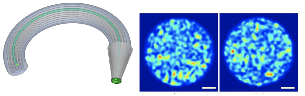
Figure 1: (left) Schematic representation of the MCF-PL. (right) Two examples of multimode pattern images obtained through the MCF.

In [4], an iterative variational method (SARA-COIL) is proposed to estimate the original image from the MCF-PL measurements. It is based on the primal-dual Condat-Vũ iterations [5, 6], for solving a sequence of constrained problems in a redundant wavelet domain. The authors show that it enables accurate reconstruction on simulated data. However, a drop on the reconstruction quality was observed on real data. Further, SARA-COIL is based on a reweighting $\ell_{1}$-scheme approximating a log-sum prior [7], coupled with multiple wavelet transforms, which leads to an overall computationally expensive approach with weak convergence guarantees.

We aim to improve the reconstruction quality, yet ensuring the reliability of the solution. Motivated by the good performance of hybrid optimization method involving neural network (NNs) in computational imaging [8, 9, 10, 11], we develop a new plug-and-play (PnP) algorithm based on the primal-dual iterations. The proposed approach solves a constrained problem, using a learned denoising NN to replace the sparsity prior. We train the NN to hold desirable Lipschitz properties ensuring the stability of the provided solution [12]. In addition, we show that the limit point of the proposed algorithm is a zero of a monotone operator. The proposed approach outperforms SARA-COIL on both simulated and real data.

The remainder of the paper is organized as follows. In Section 2 we describe the formal COIL inverse problem, and provide some backgroung on PnP in the context of monotone inclusion problems. The proposed approach is presented in Section 3. In Section 4 we evaluate the performance of the proposed PnP approach on simulated and real data.

2 Background

2.1 Multicore fibre with photonic lantern and SARA-COIL

Light patterns generated by the PL are projected onto an object (e.g., tissue) and light returned from the object (e.g., fluorescence) is detected by a single-pixel detector. We consider $M$ multimode light patterns. The $m$-th pattern (for $m\in\{1,\ldots,M\}$) produces a scalar measurement $y_{m}\in\mathbb{R}$ corresponding to the sum of the pixelwise multiplication of the pattern and the image of the object of interest. Formally, the observations $y\in{\mathbb{R}}^{M}$ are obtained as

$$y=\Phi\overline{x}+w,$$ (2.1)

where $\overline{x}\in{\mathbb{R}}^{N}$ is the unknown image (reshaped to a column vector), $\Phi\in{\mathbb{R}}^{M\times N}$ is the linear measurement operator, and $w\in{\mathbb{R}}^{M}$ is a realization of a random perturbation. Each row of $\Phi$ contains one pattern (as per Fig. 1), reshaped to a row vector. The distribution of the noise is not known exactly, but assumed to have a bounded energy, i.e., $\|w\|_{2}\leqslant\varepsilon$ for $\varepsilon>0$.

The SARA-COIL method [4] defines the estimate as

$$\widehat{x}\in\underset{\begin{subarray}{c}{x\in[0,+\infty)^{N}}\end{subarray}}{\mathrm{Argmin}}\;\;f(\Psi x)\text{ subject to }\|\Phi x-y\|_{2}\leqslant\varepsilon,$$ (2.2)

where $\Psi\in{\mathbb{R}}^{S\times N}$ is the concatenation of the first eight Daubechies wavelets transforms and the Dirac basis, and $f\colon{\mathbb{R}}^{S}\to(-\infty,+\infty]$ is a log-sum penalization function [7, 13, 14]. The authors in [4] propose to solve (2.2) using a reweighting-$\ell_{1}$ approach [7], combined with a primal-dual algorithm [5, 6]. Formally, the primal-dual algorithm is used to sequentially solve a collection of problems of the form

$$\widehat{x}\in\underset{\begin{subarray}{c}{x\in[0,+\infty)^{N}}\end{subarray}}{\mathrm{Argmin}}\;\;\|\Delta\Psi x\|_{1}\text{ subject to }\|\Phi x-y\|_{2}\leqslant\varepsilon,$$ (2.3)

where $\Delta\in{\mathbb{R}}^{S\times S}$ is a weight diagonal matrix, whose diagonal elements are chosen according to the current estimate of $\overline{x}$ (see, e.g., [14, 15] for more details). SARA-COIL showed a good performance on simulated data, but with a significant drop on real data. In addition, this method suffers from the high computational cost mentioned in the introduction. Finally, although recent works provided theoretical guarantees for some reweighted-$\ell_{1}$ approaches solving log-sum problems [16, 17, 18, 19], SARA-COIL does not satisfy the necessary conditions to ensure its convergence to a solution to (2.2).

2.2 Learning MMOs

Recently, optimization-based approaches have been made more powerful by coupling them with NN models. In particular, unfolded and PnP methods are highly efficient for solving inverse imaging problems [8, 9, 10, 11, 20, 21, 22]. In this work we focus PnP methods. In a nutshell, they consist of replacing some steps in an optimization algorithm by a NN. For image recovery, denoising NNs are often used to replace proximity operators related to the regularization (e.g., replacing the soft-thresholding operator associated with $\ell_{1}$ regularization).

Multiple works studied the PnP methods theoretical guarantees [23, 24, 12, 25, 26, 27, 28]. In general, to ensure convergence of the generated iterate sequence, the NN must be firmly non-expansive (FNE). An operator $J\colon\mathbb{R}^{N}\to\mathbb{R}^{N}$ is FNE [29] if, for every $(x,y)\in(\mathbb{R}^{N})^{2}$, $\|J(x)-J(y)\|_{2}^{2}\leqslant{\left\langle{{x-y}\mid{J(x)-J(y)}}\right\rangle}$. A few works further provide theoretical characterization of the limit point [23, 24, 12, 25].

In [12], the authors propose to use maximally monotone operator (MMO) theory to design PnP algorithms for solving monotone inclusion problems. The objective is to

$$\text{find }\widehat{x}\in\mathbb{R}^{N}\text{ such that }0\in A(\widehat{x})+B(\widehat{x}),$$ (2.4)

where $A$ and $B$ are MMOs, i.e., for every $(x_{1},u_{1})\in(\mathbb{R}^{N})^{2}$, $u_{1}\!\in\!\!A(x_{1})$ if and only if for every $x_{2}\in\mathbb{R}^{N}$ and $u_{2}\!\in\!A(x_{2})$, ${\left\langle{{x_{1}-x_{2}}\mid{u_{1}-u_{2}}}\right\rangle}\!\!\geqslant\!0$. Such problems can be solved by algorithms grounded on MMO theory, including forward-backward (FB), Douglas–Rachford (DR), primal-dual approaches [29, 30, 5, 31, 6, 32]. For these algorithms, $B$ can be handled through its resolvent operator $J_{B}=(\text{Id}+B)^{-1}$ [29]. Depending on the scheme, operator $A$ is then handled either explicitly (e.g., FB algorithm), through its resolvent operator (e.g., DR algorithm), or using further splitting (i.e., primal-dual methods).

In [12], these schemes are used to define generic PnP algorithms to solve (2.4), replacing $J_{B}$ by a learned NN $\widetilde{J}$. The authors showed that if $\widetilde{J}$ is FNE, then any sequence $(x_{n})_{n\in\mathbb{N}}$ generated by the resulting PnP algorithm converges to a limit point $\widehat{x}$. They proposed a FB-PnP algorithm for solving (2.4). To the best of our knowledge, this MMO/PnP perspective has not been used yet with other iterative schemes. In this work, we develop a new primal-dual PnP method for solving monotone inclusion problems involving linear operators.

3 Proposed Primal-Dual PnP algorithm

SARA-COIL solves a collection of problems of the form (2.3), which is a particular case of (2.4) with

$$A=\Phi^{\top}N_{{\mathcal{B}}_{2}(y,\varepsilon)}\Phi,\text{ and }B=\partial\|\Delta\Psi\cdot\|_{1}+N_{[0,+\infty)^{N}},$$ (3.1)

where ${\mathcal{B}}_{2}(y,\varepsilon)$ is the $\ell_{2}$-ball centered in $y$ with radius $\varepsilon$, and $\Phi^{\top}$ denotes the transpose of matrix $\Phi$. The normal cone $N_{S}$ of a subset $S$ of a Hilbert space ${\mathcal{H}}$, equipped with an inner product ${\left\langle{{\cdot}\mid{\cdot}}\right\rangle}$, is defined as $N_{S}\colon x\mapsto\{u\in{\mathcal{H}}\mid(\forall y\in S)\,{\left\langle{{u}\mid{y-x}}\right\rangle}\leqslant 0\}$ if $x\in S$, and $\varnothing$ otherwise.

In this work, we propose to learn a generic operator $B$, i.e.,

$$\text{find }\widehat{x}\text{ such that }0\in\Phi^{\top}N_{{\mathcal{B}}_{2}(y,\varepsilon)}\Phi(\widehat{x})+B(\widehat{x}).$$ (3.2)

An efficient algorithm for solving Problem (3.2) is the primal-dual Condat-Vũ algorithm. The convergence proof of this algorithm is based on MMO theory, and it has the advantage that it does not require operator $\Phi$ to be inverted.

In this work, similarly to [12], we propose to characterize $B$ through its resolvent. Let $\widetilde{J}_{\theta}$ be an operator parameterized by a vector $\theta$. If $\widetilde{J}_{\theta}=\frac{\text{Id}+Q_{\theta}}{2}$, where $Q_{\theta}$ is a $1$-Lipschitz operator, then $\widetilde{J}_{\theta}$ is the resolvent of a MMO $\widetilde{B}$. By modelling $Q_{\theta}$ as a NN, the model parameter vector $\theta$ can thus be learnt to provide an optimal choice for the MMO regularizer. The resulting PnP method is given in Algorithm 1. Then, the following convergence result naturally follows from [5, 6] .

Theorem 3.1

Let $(x_{k})_{k\in\mathbb{N}}$ be a sequence generated by Algorithm 1. Assume that $\tau\sigma\|\Phi\|^{2}<1$, and that $\widetilde{J}_{\theta}$ is chosen as described above. Let $\widetilde{B}$ be the MMO equal to $\widetilde{J}_{\theta}^{-1}-\operatorname{Id}$. Assume that there exists at least a solution $\widehat{x}$ to the inclusion

$$0\in\Phi^{\top}N_{{\mathcal{B}}_{2}(y,\varepsilon)}\Phi(\widehat{x})+\tau^{-1}\widetilde{B}(\widehat{x}).$$ (3.3)

Then $(x_{k})_{k\in\mathbb{N}}$ converges to a such a solution.

In particular, this theorem shows that $B$ is equal to $\widetilde{B}$ up to the multiplicative factor $1/\tau$.

Algorithm 1 PnP primal-dual algorithm for solving (3.3)

  Let $(x_{0},v_{0})\in\mathbb{R}^{N}\times\mathbb{R}^{M}$ and $(\tau,\sigma)\in(0,+\infty)^{2}$.

  for $k=0,1,\ldots$ do

     $\widetilde{x}_{k}=x_{k}-\tau\Phi^{\top}u_{k}$

     $x_{k+1}=\widetilde{J}_{\theta}\big{(}\widetilde{x}_{k}\big{)}$

     $\widetilde{u}_{k}=u_{k}+\sigma\Phi(2x_{k+1}-x_{k})$

     $u_{k+1}=\widetilde{u}_{k}-\sigma\operatorname{proj}_{{\mathcal{B}}_{2}(y,\varepsilon)}\big{(}\widetilde{u}_{k}/\sigma^{-1}\big{)}$

  end for

4 Experimental results

4.1 Training

Similarly to [12], we train $\widetilde{J}_{\theta}$, on a denoising task, to satisfy the desired 1-Lipschitz condition. Let $(\overline{x}_{i},z_{i})_{i\in\mathbb{I}}$ be a set of pairs of ground truth images $(\overline{x}_{i})_{i\in\mathbb{I}}$ and associated noisy images $(z_{i})_{i\in\mathbb{I}}$. For every $i\in\mathbb{I}$, we have $z_{i}=\overline{x}_{i}+\upsilon w_{i}$, where $w_{i}\in\mathbb{R}^{N}$ is a realization of an additive standard normal random variable, and $\upsilon>0$.

The vector of parameters $\theta$ of the NN is learned so as to

$$\underset{\begin{subarray}{c}{\theta}\end{subarray}}{\mathrm{minimize}}\;\;\dfrac{1}{\sharp\,\mathbb{I}}\sum_{i\in\mathbb{I}}\Big{(}\|\widetilde{J}_{\theta}(z_{i})-\overline{x}_{i}\|_{2}^{2}+\lambda\max\big{\{}\|\nabla Q_{\theta}(z_{i})\|_{S}^{2},1-\delta\big{\}}\Big{)}.$$ (4.1)

The first term is the standard $\ell^{2}$ loss for training denoising NNs, while the second term is a Jacobian regularization introduced in [12] to ensure that $Q_{\theta}=2\widetilde{J}_{\theta}-\text{Id}$ is $1$-Lipschitz. Precisely, for every $i\in\mathbb{I}$, $\nabla Q_{\theta}(z_{i})$ denotes the Jacobian of $Q_{\theta}$ computed at $z_{i}$, and $(\lambda,\delta)\in(0,+\infty)^{2}$ are regularization parameters. The spectral norm $\|\nabla Q_{\theta}(z_{i})\|_{S}$ is computed using a power method coupled with back-propagation.

We train three DnCNN networks [33] considering different noise levels $\upsilon\in\{5,10,20\}$, on NVIDIA GeForce RTX 2080 Ti GPUs provided by [34]. We use Adam [35] optimizer on $60\%$ images of the ImageNet [36] validation dataset, converted to grayscale images with values in $[0,255]$, with batch size $40$, patch size $64\times 64$, learning rate $5\times 10^{-5}$, and a scheduler reducing the learning rate by $10\%$ when validation runs without improvement. We further use $20\%$ of the ImageNet validation dataset as test set, and the remainder is used for validation during the training.

Training results are summarized in Table 1, where the $10,000$ images of our test dataset are used to check that $\max_{x}\|\nabla Q(x)\|_{S}\leqslant 1$ and evaluate the PSNR values for the denoising task. For each value of $\upsilon$, we choose the smallest $\lambda$ needed to ensure that the previous inequality holds.

Table 1: Training results on denoising problem.

$\upsilon$	$\lambda$	$\max_{x}\|\nabla Q(x)\|$	PSNR (dB)
$5$	$10^{-3}$	$0.9963$	$36.65$
$10$	$5\times 10^{3}$	$0.9952$	$32.12$
$20$	$10^{-2}$	$0.9797$	$28.40$

4.2 Experimental setting

We use the same MCF-PL setting as in [4, 37]. The PL was added at one end of $\sim 3$m of MCF with $121$ single-mode cores in a $11\times 11$ square array. Each core was individually excited using coherent $514$nm laser light, generating $11^{2}=121$ different multimode patterns of light. To augment the total measurement number $M$, we also consider a setting where the fiber was rotated $9$ times by $40^{\circ}$ around the optical axis, creating a total of $121\times 9=1089$ patterns. The measurement operator $\Phi$ corresponds to the concatenation of the $M=121$ or $M=1089$ patterns, each of size $N=377\times 377$.

These patterns are used for both simulated and experimental data. For simulated data, measurements are created according to Model (2.1), using the $1089$ patterns and a noise level yielding an input SNR of $30$dB. For experimental data, measurements were acquired using the fiber and a single-pixel camera, where the object was moved into the beam path, and the magnitude of the light transmitted through the object was recorded by a detector. We highlight the fact that the MCF was intentionally moved and deformed significantly between pattern calibration and imaging experiments, to further highlight the stability of the PL approach (see [4] for more details). The field of view of all reconstructions using experimentally measured data is $0.9$mm$\times 0.9$mm in the object plane.

Table 2: Simulated data: Average results obtained for PnP-COIL.

$\upsilon$	PSNR (dB)	SSIM
$5$	$37.81$ $(\pm 2.49)$	$0.698$ $(\pm 0.012)$
$10$	$37.61$ $(\pm 2.08)$	$0.687$ $(\pm 0.024)$
$20$	$36.81$ $(\pm 2.42)$	$0.672$ $(\pm 0.022)$
SARA-COIL	$30.72$ $(\pm 1.38)$	$0.544$ $(\pm 0.023)$

Ground truth	SARA-COIL	PnP – $\upsilon=5$	PnP – $\upsilon=10$	PnP – $\upsilon=20$

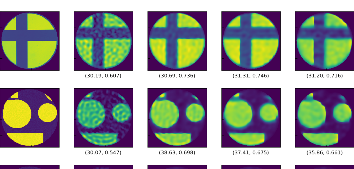
	$(30.19,0.607)$	$(30.69,0.736)$	$(31.31,0.746)$	$(31.20,0.716)$

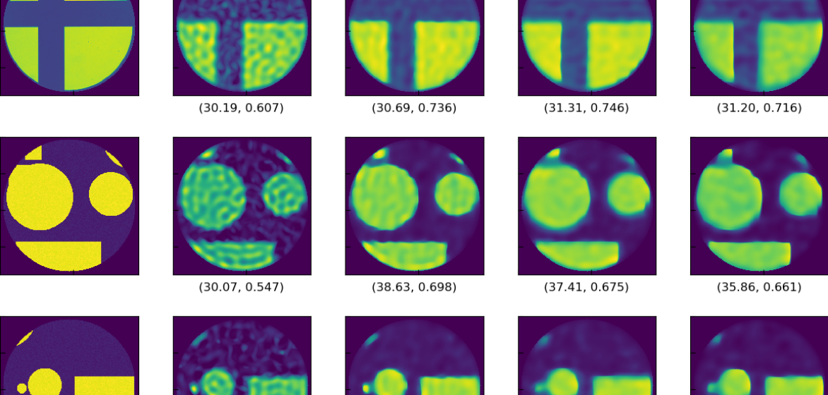
	$(30.07,0.547)$	$(38.63,0.698)$	$(37.41,0.675)$	$(35.86,0.661)$

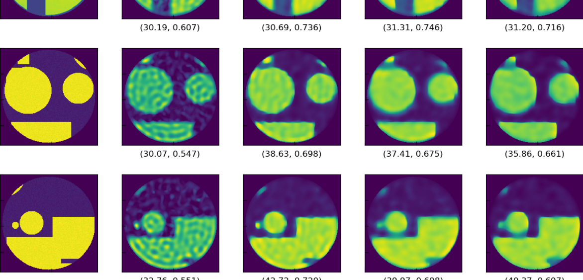
	$(32.76,0.551)$	$(42.72,0.720)$	$(39.97,0.698)$	$(40.37,0.697)$

Figure 2: Simulated data: Comparison between ground truth, results from SARA-COIL, and results from proposed PnP-COIL with DnCNNs trained on noise levels $\upsilon\in\{5,10,20\}$. Values below images indicate (PSNR, SSIM).

4.3 Simulated data

We validate our primal-dual PnP algorithm on simulated COIL data (dubbed PnP-COIL). To this aim, we generate $50$ images with geometric patterns. Examples are shown in Figure 2 (left column). Average PSNR and SSIM values (with associated standard deviation) are reported in Table 2. For these results, we fixed $\varepsilon=50$ in Algorithm 1. Quantitative results are very similar for the three trained DnCNNs, showing that PnP-COIL is fairly stable with respect to the training noise level. Visual inspections for three of these images are reported in Figure 2, for images obtained with the three trained DnCNNs and with SARA-COIL [4]. We observe that PnP-COIL outperforms SARA-COIL on all examples, although the network has been trained on a very different dataset. Further improvement could certainly be obtained by finetuning the network. Finally, we observed that PnP-COIL usually requires less iterations than SARA-COIL to reach convergence.

Ground truth	$M=121$	$M=1089$

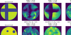
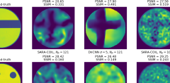
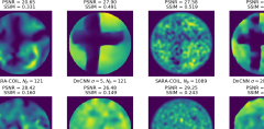
Ground truth	$M=1089$

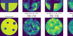
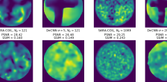
Figure 3: Experimental data: Ground truth and reconstructions obtained with SARA-COIL considering $M=121$ and $M=1089$ patterns for cross image (top) and $M=1089$ patterns for dots image (bottom).

$\qquad\varepsilon=2\qquad$	$\qquad\varepsilon=2.5\qquad$	$\qquad\varepsilon=3\qquad$	$\qquad\varepsilon=3.5\qquad$
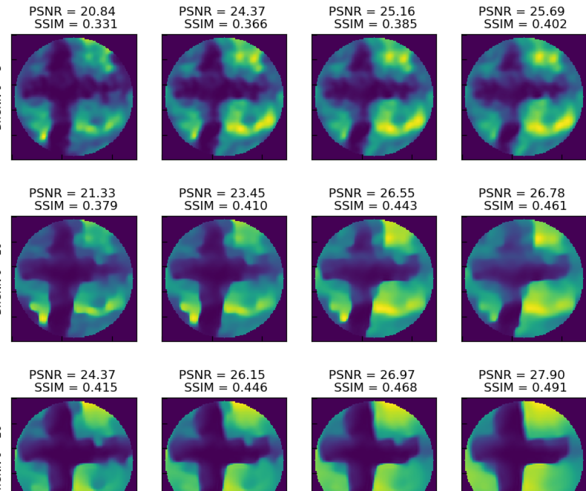
$\qquad\;\;(20.84,0.331)\;\qquad$	$\qquad\qquad\;(24.37,0.366)\;\qquad$	$\qquad\;\;\;(25.16,0.470)\;\qquad$	$\qquad\;\;\;\;(25.69,0.402)\;\qquad$
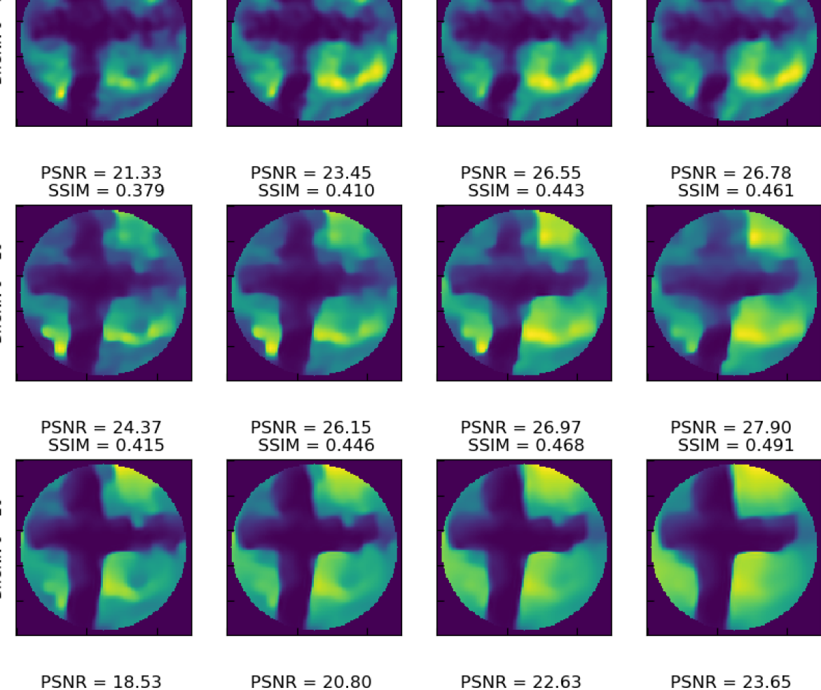
$\;\;(21.33,0.379)\;$	$\;\;(23.45,0.410)\;$	$\;\;(26.55,0.443)\;$	$\;\;(26.78,0.461)\;$
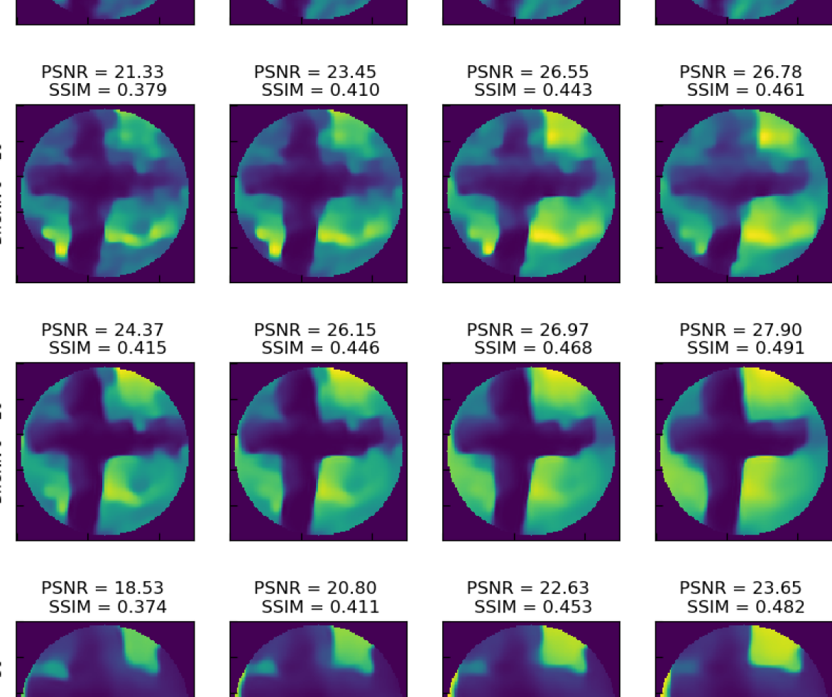
$\;\;(24.37,0.415)\;$	$\;\;(26.15,0.446)\;$	$\;\;(26.97,0.468)\;$	$\;\;(27.90,0.491)\;$

Figure 4: Experimental data: Reconstructions for cross image with $M=121$, obtained with the proposed PnP-COIL, considering different parameters: top to bottom $\upsilon\in\{5,10,20\}$, and left to right $\varepsilon\in\{2,2.5,3,3.5\}$.

$\qquad\varepsilon=6\qquad$	$\qquad\varepsilon=7\qquad$	$\qquad\varepsilon=8\qquad$	$\qquad\varepsilon=9\qquad$
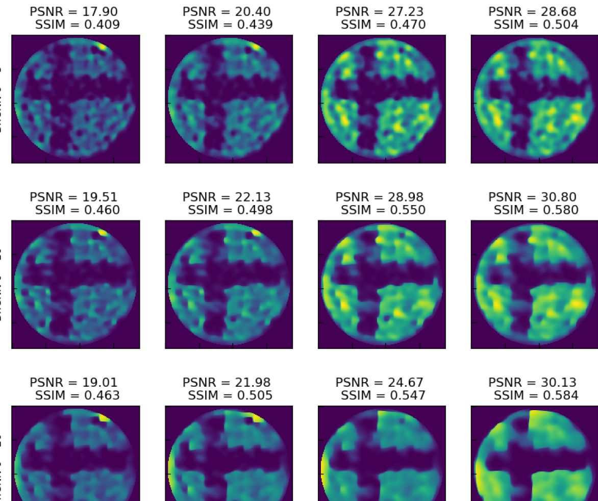
$\qquad\;\;(17.90,0.409)\;\qquad$	$\qquad\quad\;\;(20.40,0.439)\;\qquad$	$\qquad\quad\quad\;(27.23,0.470)\;\qquad$	$\qquad\;\;\;\;(28.68,0.504)\;\qquad$
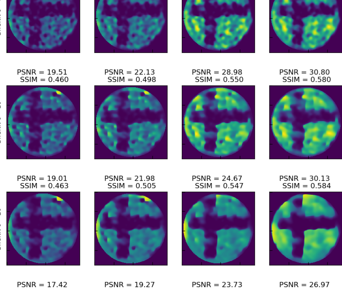
$\;\;(19.51,0.460)\;$	$\;\;(22.13,0.498)\;$	$\;\;(28.98,0.550)\;$	$\;\;(30.80,0.580)\;$
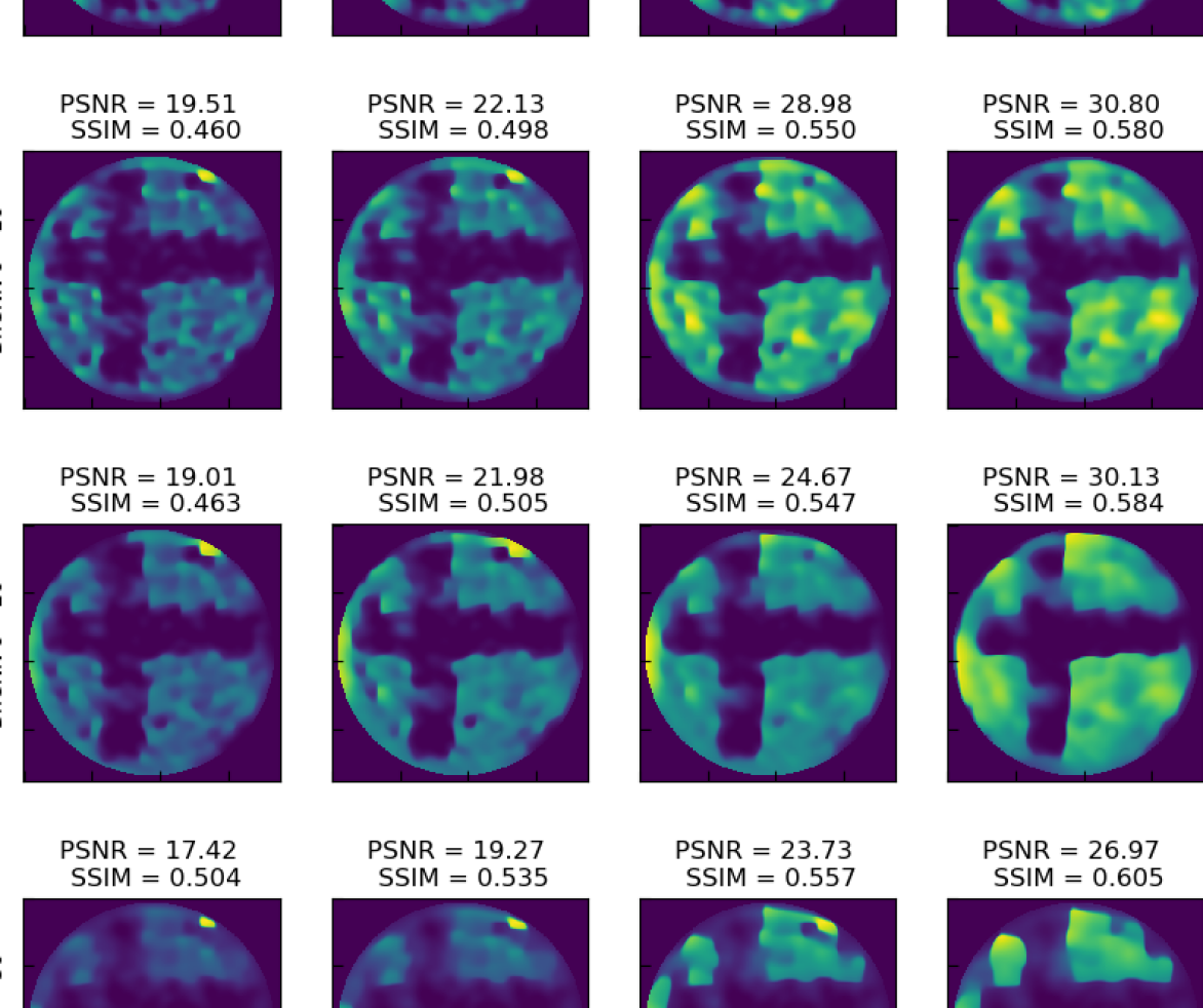
$\;\;(19.01,0.463)\;$	$\;\;(21.98,0.505)\;$	$\;\;(24.67,0.547)\;$	$\;\;(30.13,0.584)\;$

Figure 5: Experimental data: Reconstructions for cross image with $M=1089$, obtained with the proposed PnP-COIL, considering different parameters: top to bottom $\upsilon\in\{5,10,20\}$, and left to right $\varepsilon\in\{6,7,8,9\}$.

$\qquad\varepsilon=12\qquad$	$\qquad\varepsilon=13\qquad$	$\qquad\varepsilon=14\qquad$	$\qquad\varepsilon=15\qquad$
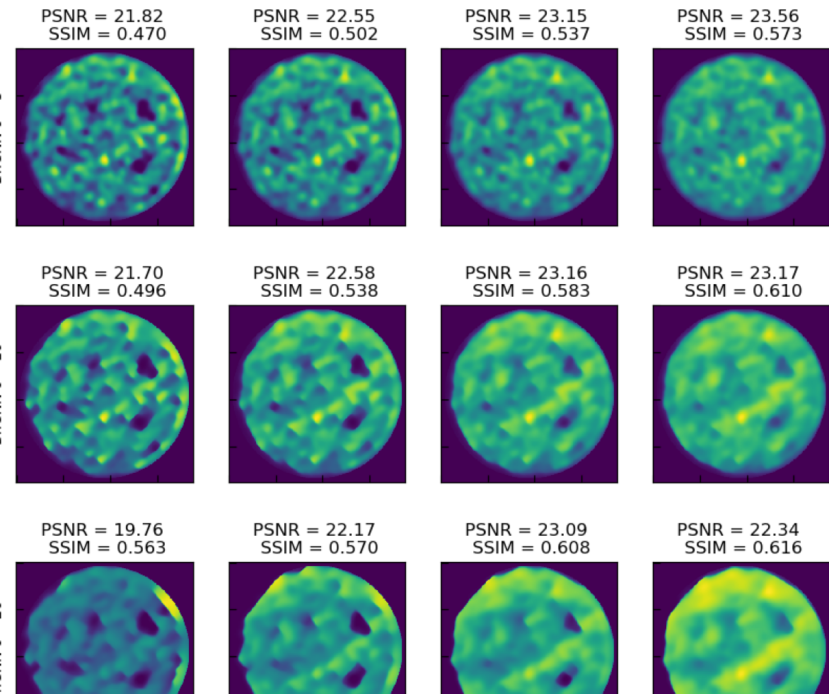
$\qquad\;\;(21.82,0.470)\;\qquad$	$\qquad\quad\;\;(22.55,0.502)\;\qquad$	$\qquad\quad\;\;\;(23.15,0.537)\;\qquad$	$\qquad\quad\;\;(23.56,0.573)\;\qquad$
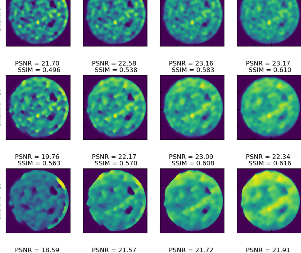
$\;\;(21.70,0.496)\;$	$\;\;(22.58,0.538)\;$	$\;\;(23.16,0.583)\;$	$\;\;(23.17,0.610)\;$
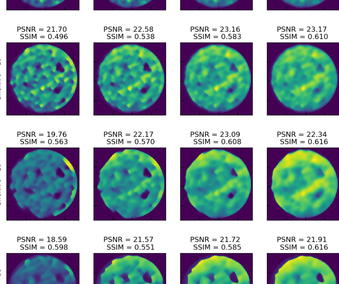
$\;\;(19.76,0.563)\;$	$\;\;(22.17,0.570)\;$	$\;\;(23.09,0.608)\;$	$\;\;(22.34,0.616)\;$

Figure 6: Experimental data: Reconstructions for dots image with $M=1089$, obtained with the proposed PnP-COIL, considering different parameters: top to bottom $\upsilon\in\{5,10,20\}$, and left to right $\varepsilon\in\{12,13,14,15\}$.

4.4 Experimental data

We validate the proposed algorithm on real data, acquired as per Section 4.2, using two images: cross and dots (Figure 3-left). The reconstructions obtained with SARA-COIL for cross are reported in Figure 3. Reconstructions using PnP-COIL are given in Figures 4-6. In each case, we show the results obtained considering the NNs trained on different noise levels $\upsilon$, for different radius of the $\ell_{2}$-ball $\varepsilon$ in (3.2). For all cases, the reconstructed images become smoother when both parameters $(\upsilon,\varepsilon)$ increase. For the cross example, we observe that the proposed primal-dual PnP method leads to higher accuracy in the reconstruction than SARA-COIL (see Figures 4 and 5). For the dots example, we see in Figure 6 that the proposed approach enables finding the 4 dots in the image when $M=1089$, while SARA-COIL could barely see one of them.

5 Conclusion

In this work, we have introduced a new primal-dual PnP algorithm for solving monotone inclusion problems, in the context of computational optical imaging. The proposed approach enables to handle non-smooth data-fidelity terms involving a linear operator, e.g. an ellipsoidal constraint. We showed the outperformance of the proposed PnP-COIL approach on simulated and real COIL data with respect to the state-of-the art variational approach.

References

- [1] H. A. C. Wood, K. Harrington, T. A. Birks, J. C. Knight, and J. M. Stone, “Highresolution air-clad imaging fibers,” Opt. Lett., vol. 43, pp. 5311–5314, 2018.
- [2] A. R. Akram, S. V. Chankeshwara, E. Scholefield, T. Aslam, N. McDonald, A. Megia-Fernandez, A. Marshall, B. Mills, N. Avlonitis, T. H. Craven, A. M. Smyth, D. S. Collie, Gray C., N. Hirani, A.T. Hill, J.R. Govan, T. Walsh, C. Haslett, M. Bradley, and K. Dhaliwal, “In situ identification of gram-negative bacteria in human lungs using a topical fluorescent peptide targeting lipid,” A. Sci. Transl. Med., vol. 10, pp. eaal0033, 2018.
- [3] T. A. Birks, I. Gris-Sánchez, S. Yerolatsitis, S. G. Leon-Saval, and R. R. Thomson, “The photonic lantern,” Adv. Opt. Photon., vol. 7, pp. 107–167, 2015.
- [4] D. Choudhury, D. K. McNicholl, A. Repetti, I. Gris-Sánchez, S. Li, D. B. Phillips, G. Whyte, T. A. Birks, Y. Wiaux, , and R. R. Thomson, “Computational optical imaging with a photonic lantern,” Nat. Commun., vol. 11, no. 1, pp. 5217, 2020.
- [5] L. Condat, “A primal–dual splitting method for convex optimization involving Lipschitzian, proximable and linear composite terms,” J. Optim. Theory Appl., vol. 158, no. 2, pp. 460–479, 2013.
- [6] B. C. Vũ, “A splitting algorithm for dual monotone inclusions involving cocoercive operators,” Adv. Comput. Math., vol. 38, no. 3, pp. 667–681, 2013.
- [7] E. J. Candès, “Compressive sampling,” in Proceedings of the international congress of mathematicians. Madrid, Spain, 2006, vol. 3, pp. 1433–1452.
- [8] J. Adler and O. Öktem, “Learned primal-dual reconstruction,” IEEE Trans. Med. Imag., vol. 37, no. 6, pp. 1322–1332, 2018.
- [9] A. Teodoro, J. M. Bioucas-Dias, and M. A. T. Figueiredo, “Image restoration and reconstruction using targeted plug-and-play priors,” IEEE Trans. Comput. Imag., vol. 5, no. 4, pp. 675–686, 2019.
- [10] R. Ahmad, C. A. Bouman, G. T. Buzzard, S. Chan, S. Liu, E. T. Reehorst, and P. Schniter, “Plug-and-play methods for magnetic resonance imaging: Using denoisers for image recovery,” IEEE Signal Process. Mag, vol. 37, no. 1, pp. 105–116, 2020.
- [11] K. Zhang, Y. Li, W. Zuo, L. Zhang, L. Van Gool, and R. Timofte, “Plug-and-play image restoration with deep denoiser prior,” IEEE Trans. Pattern Anal. Mach. Intell., 2021.
- [12] J.-C. Pesquet, A. Repetti, M. Terris, and Y. Wiaux, “Learning maximally monotone operators for image recovery,” SIAM J. Imaging Sci., vol. 14, no. 3, pp. 1206–1237, 2021.
- [13] E. J. Candès, M. B. Wakin, and S. Boyd, “Enhancing sparsity by reweighted minimization,” J. Fourier Anal. Appl., vol. 14, pp. 877–905, 2007.
- [14] R. E. Carrillo, J. D. McEwen, D. Van De Ville, J.-P. Thiran, and Y. Wiaux, “Sparsity averaging for compressive imaging,” IEEE Signal Process. Lett., vol. 20, no. 6, pp. 591–594, 2013.
- [15] A. Onose, R. E. Carrillo, A. Repetti, J. D. McEwen, J.-P. Thiran, J.-C. Pesquet, and Y. Wiaux, “Scalable splitting algorithms for big-data interferometric imaging in the ska era,” Mon. Not. R. Astron. Soc., vol. 462, no. 4, pp. 4314–4335, 2016.
- [16] A. Repetti and Y. Wiaux, “Variable metric forward-backward algorithm for composite minimization problems,” SIAM J. Optim., vol. 31, no. 2, pp. 1215–1241, 2021.
- [17] J. Geiping and M. Moeller, “Composite optimization by nonconvex majorization-minimization,” SIAM J. Imaging Sci., vol. 11, no. 4, pp. 2494–2598, 2018.
- [18] P. Ochs, A. Dosovitskiy, T. Brox, and T. Pock, “On iteratively reweighted algorithms for nonsmooth nonconvex optimization in computer vision,” SIAM J. Imaging Sci., vol. 8, no. 1, pp. 331–372, 2015.
- [19] P. Ochs, J. Fadili, and T. Brox, “Non-smooth non-convex Bregman minimization: Unification and new algorithms,” J. Optim. Theory. Appl., vol. 181, no. 1, pp. 244–278, 2019.
- [20] D. Ren, W. Zuo, D. Zhang, L. Zhang, and M.-H. Yang, “Simultaneous fidelity and regularization learning for image restoration,” IEEE Trans. Pattern Anal. Mach. Intell., vol. 43, no. 1, pp. 284–299, 2019.
- [21] C. Bertocchi, E. Chouzenoux, M.-C. Corbineau, J.-C. Pesquet, and M. Prato, “Deep unfolding of a proximal interior point method for image restoration,” Inverse Problems, vol. 36, no. 3, pp. 034005, 2020.
- [22] M. Jiu and N. Pustelnik, “A deep primal-dual proximal network for image restoration,” IEEE J. Sel. Topics Signal Process., vol. 15, no. 2, pp. 190–203, 2021.
- [23] M. Terris, A. Repetti, J.-C. Pesquet, and Y. Wiaux, “Building firmly nonexpansive convolutional neural networks,” in IEEE International Conference on Acoustics, Speech and Signal Processing (ICASSP). IEEE, 2020, pp. 8658–8662.
- [24] R. Cohen, M. Elad, and P. Milanfar, “Regularization by denoising via fixed-point projection (RED-PRO),” SIAM J. Imaging Sci., vol. 14, no. 3, pp. 1374–1406, 2021.
- [25] J. Hertrich, S. Neumayer, and G. Steidl, “Convolutional proximal neural networks and plug-and-play algorithms,” Linear Algebra Appli., vol. 631, pp. 203–234, 2021.
- [26] X. Xu, Y. Sun, J. Liu, B. Wohlberg, and U. S. Kamilov, “Provable convergence of plug-and-play priors with MMSE denoisers,” IEEE Signal Process. Lett., vol. 27, pp. 1280–1284, 2020.
- [27] R. Laumont, V. De Bortoli, A. Almansa, J. Delon, A. Durmus, and M. Pereyra, “On maximum a posteriori estimation with plug & play priors and stochastic gradient descent,” J. Math. Imaging Vision, pp. 1–24, 2023.
- [28] S. Hurault, A. Leclaire, and N. Papadakis, “Proximal denoiser for convergent plug-and-play optimization with nonconvex regularization,” in International Conference on Machine Learning. PMLR, 2022, pp. 9483–9505.
- [29] H. H. Bauschke and P. L. Combettes, Convex analysis and monotone operator theory in Hilbert spaces, Springer, 2017.
- [30] P. L. Combettes and J.-C. Pesquet, “Proximal splitting methods in signal processing,” in Fixed-point algorithms for inverse problems in science and engineering, pp. 185–212. Springer, 2011.
- [31] N. Komodakis and J.-C. Pesquet, “Playing with duality: An overview of recent primal-dual approaches for solving large-scale optimization problems,” IEEE Signal Process. Mag, vol. 32, no. 6, pp. 31–54, 2015.
- [32] P. L. Combettes and J.-C. Pesquet, “Fixed point strategies in data science,” IEEE Trans. Image Process., vol. 69, pp. 3878–3905, 2021.
- [33] K. Zhang, W. Zuo, Y. Chen, D. Meng, and L. Zhang, “Beyond a Gaussian denoiser: Residual learning of deep CNN for image denoising,” IEEE Trans. Image Process., vol. 26, no. 7, pp. 3142–3155, 2017.
- [34] J. Fix, S. Vialle, R. Hellequin, C. Mercier, P. Mercier, and J.-B. Tavernier, “Feedback from a data center for education at CentraleSupélec engineering school,” in 2022 IEEE International Parallel and Distributed Processing Symposium Workshops (IPDPSW), 2022, pp. 330–337.
- [35] D. P. Kingma and J. Ba, “Adam: A method for stochastic optimization,” Tech. Rep., 2014, 10.48550/arxiv.1412.6980.
- [36] O. Russakovsky, J. Deng, H. Su, J. Krause, S. Satheesh, S. Ma, Z. Huang, A. Karpathy, A. Khosla, M. Bernstein, A. C. Berg, and L. Fei-Fei, “Imagenet large scale visual recognition challenge,” Tech. Rep., 2014, 10.48550/arxiv.1409.0575.
- [37] R. R. Thomson, D. McNicholl, and A. Repetti, “Supporting data for “computational optical imaging with a photonic lantern” by Choudhury et al,” 2020, DOI:10.17861/a1bebd55-b44f-4b34-82c0-c0fe925762c6.