Pseudorandom unitaries are neither real nor sparse nor noise-robust

Abstract

Pseudorandom quantum states (PRSs) and pseudorandom unitaries (PRUs) possess the dual nature of being efficiently constructible while appearing completely random to any efficient quantum algorithm. In this study, we establish fundamental bounds on pseudorandomness. We show that PRSs and PRUs exist only when the probability that an error occurs is negligible, ruling out their generation on noisy intermediate-scale and early fault-tolerant quantum computers. Additionally, we derive lower bounds on the imaginarity and coherence of PRSs and PRUs, rule out the existence of sparse or real PRUs, and show that PRUs are more difficult to generate than PRSs. We introduce pseudoresource, where states of with low amount of a given resource masquerade as high-resource states. We define pseudocoherence, pseudopurity and pseudoimaginarity, and identify three distinct types of pseudoresources in terms of their masquerading capabilities. Our work also establishes rigorous bounds on the efficiency of property testing, demonstrating the exponential complexity in distinguishing real quantum states from imaginary ones, in contrast to the efficient measurability of unitary imaginarity. Lastly, we show that the transformation from a complex to a real model of quantum computation is inefficient, in contrast to the reverse process, which is efficient. Our results establish fundamental limits on property testing and provide valuable insights into quantum pseudorandomness.

Randomness is a key resource for quantum information processing [1, 2, 3, 4, 5, 6, 7, 8, 9, 10, 11]. However, a simple counting argument reveals that preparing completely random quantum states is computationally intractable. Thus, a core challenge lies in identifying quantum states and unitaries that can be efficiently prepared while remaining indistinguishable from truly random ones.

To solve this problem, the concepts of pseudorandom quantum states (PRSs) and pseudorandom unitaries (PRUs) have been introduced [1]. There is no efficient quantum algorithm that can distinguish Haar random states and unitaries from PRSs and PRUs, respectively, yet we can efficiently prepare them. Further, PRSs can be generated with much shorter circuits compared to state designs [1, 12, 13] and have been shown to be a weaker primitive than one-way functions [14]. They have also been used to design cryptographic functionalities such as commitment schemes [15, 16, 17], pseudo one-time pads [15, 16, 17] and pseudorandom strings [18]. There is an ongoing search to identify PRSs with as simple a structure as possible. Recent work showed that PRSs can have logarithmic entanglement [13] and require at least a linear number of non-Clifford gates [19]. However, for most other properties, the minimal requirements to generate PRSs or PRUs are unknown.

Imaginarity and coherence are key resources in quantum information processing, playing crucial roles in achieving a quantum advantage in various tasks. Imaginarity characterizes the degree to which states and operations require non-real numbers for their description. Surprising differences between real and complex descriptions of quantum mechanics can arise [20, 21, 22] and there are tasks that can be accomplished only with operations described by non-real numbers [23, 24, 25]. On the other hand, coherence, which measures the degree of being in a superposition, is a fundamental resource in quantum processing [26, 27, 28, 29, 30, 31] that is intricately linked to entanglement [32, 33], circuit complexity [34] and serves as a vital ingredient in quantum algorithms [35, 36, 37, 38].

Given their importance, can we verify whether coherence or imaginarity are actually present in a quantum state or unitary? For such tasks, the concept of property testing has been developed [39, 40, 41]. This concept has been studied extensively for other properties [42, 43, 44, 45, 46, 47, 48, 13].

Here, we provide fundamental bounds on PRSs, PRUs, and testing for imaginarity and coherence as a function of the number of qubits $n$. We show that the number of copies needed to test the imaginarity of states scales as $\Omega(2^{n/2})$ with the number of qubits $n$, while for unitaries we require only $O(1)$ copies. For coherence, we provide bounds on the number of copies needed for testing as a function of coherence of the state and unitary. This lower bounds the coherence of PRUs as $\omega(\log(n))$ and their imaginarity as $1-\text{negl}(n)$. With our results, we rule out the existence of real and sparse PRUs. Further, we show that PRSs and PRUs are not robust to noise, with a maximal depolarizing noise probability $p=\text{negl}(n)$. We introduce pseudoresource ensembles that mimic states with high resource value using states with a only a low amount of the given resource, and identify three classes of pseudoresources. Finally, we apply our results to show that there is no efficient way to transform from a complex mode of quantum computing to a real one. Our work establishes rigorous limits on property testing and the generation of pseudorandomness.

I Preliminaries

A keyed family of quantum states is considered pseudorandom if it can be generated efficiently and appears statistically indistinguishable from Haar random states to an observer with limited computational resources. More precisely, a family of PRSs is a set of states $\{|\phi_{k}\rangle\}_{k\in\mathcal{K}}$ of some key space $\mathcal{K}$ which suffices two conditions: First, they can be efficiently prepared on quantum computers. Second, given $t=\text{poly}(n)$ copies of the state, they are indistinguishable from Haar random quantum states $S(\mathcal{H})$ of an $n$-qubit Hilbert space $\mathcal{H}$, for any efficient quantum algorithm [1]. Similarly, one can also define PRUs. A family of unitary operators is considered pseudorandom if it is both efficiently computable and indistinguishable from Haar random unitary operators for an observer with bounded computational power. For details, refer to supplementary material (SM) A.

Property testing checks whether a given state has a particular property or resource $Q$. In particular, given $t$ copies of $|\psi\rangle$, we want to determine whether $|\psi\rangle$ has $Q(|\psi\rangle)\leq\beta$, where $\beta$ is the threshold for the property and $Q(|\psi\rangle)$ is a resource measure with $Q(|\psi\rangle)\geq 0$. The property tester accepts when $Q(|\psi\rangle)\leq\beta$, and rejects when $Q(|\psi\rangle)\geq\delta$, where $\delta$ is the rejection threshold, which is chosen as $\delta>\beta$. A formal definition of property testing is given in Def. 1 and a comprehensive summary of sample complexity for testing various properties.

Property $Q$	Pure states	Unitaries
Purity	$O(1)$ [49]	$O(1)$
Entanglement	$O(1)$ [50]	$O(1)$ [43]
Nonstabilizerness	$O(1)$ [44]	$O(1)$ [44]
Coherence	$O(1)$ [Prop. 1 in SM]	$O(1)$ [29]
Imaginarity	$\Omega(2^{n/2})$ [Thm. 2]	$O(1)$ [51]

Table 1: Copies $M$ needed for tester $\mathcal{A}_{Q}$ for the properties imaginarity, entanglement, nonstabilizerness, coherence and purity, where we regard pure states and unitaries. Here, we assume $\beta=0$, $\delta=\Omega(1)$ for the tester and choose a representative measure with the best known protocol for each property. Further details in SM K.

II Noise

PRSs and PRUs physically prepared on quantum computers are subject to noise originating from the environment or imperfect experimental control. One can characterize the degree of noise via the property of purity $\gamma=1-\text{tr}(\rho^{2})$ of a state $\rho$ [52]. It has been shown that PRSs must have a purity close to $1$ up to a negligible function [16]. As we now show, PRSs and PRUs are very fragile with respect to noise channels:

Theorem 1 (PRSs and PRUs are not robust to noise (SM B)).

Any ensemble of unitaries or states subject to a single-qubit depolarizing noise channel $\Lambda(X)=(1-p)X+p\mathrm{tr}(X)I_{1}/2$ can be PRSs and PRUs only with at most $p=\mathrm{negl}(n)$ depolarizing probability.

Theorem 1 is proven via the SWAP test [49]. In particular, any state or unitary subject to a local depolarizing channel with $p=\Omega(1/\text{poly}(n))$ noise probability can be efficiently distinguished from Haar random states or unitaries.

III Imaginarity of states

Next, we discuss the property of imaginarity. An $n$-qubit quantum state $\rho$ is non-imaginary or real when all the coefficients in the expansion

$$\rho=\sum_{k,\ell}\rho_{k,\ell}|k\rangle\langle\ell|\,$$ (1)

are real, i.e. $\rho_{k,\ell}\in\mathbb{R}$ for all $k,\ell$. Note that here we do not allow for flag qubits that serve as an indicator of imaginarity as used in the rebit model of quantum computation [53]. Further note that imaginarity depends on the chosen canonical basis of the system. For example, redefining the computational basis from $|0\rangle,|1\rangle$ to $|+y\rangle,|-y\rangle$, where $|\pm y\rangle=\frac{1}{\sqrt{2}}(|0\rangle\pm i|1\rangle)$, changes a real state into an imaginary one. Here, we make the usual choice to define imaginarity with respect to the canonical computational basis $|0\rangle$ and $|1\rangle$.

The degree to which a state $\rho$ is imaginary can be quantified using measures of imaginarity such as the robustness of imaginarity [54, 20]

$$R(\rho)=\min_{\tau}\left\{s\geq 0:\frac{\rho+s\tau}{1+s}\,\text{real}\right\}=\frac{1}{2}\|\rho-\rho^{T}\|_{1}$$ (2)

where the minimization is taken over all quantum states $\tau$ and $\|A\|_{1}=\mathrm{tr}(\sqrt{AA^{\dagger}})$ denotes the trace norm. We now consider the imaginarity of pure states $\rho=|\psi\rangle\langle\psi|$

$$\mathcal{I}(|\psi\rangle)\equiv R(|\psi\rangle)^{2}=1-|\langle\psi|\psi^{*}\rangle|^{2}\,$$ (3)

where $\mathcal{I}=0$ only for real states and $0\leq\mathcal{I}\leq 1$. Here, $|\psi^{\ast}\rangle$ indicates the complex conjugate of $|\psi\rangle$ and we used $\frac{1}{2}\left\||\psi\rangle\langle\psi|-|\phi\rangle\langle\phi|\right\|_{1}=\sqrt{1-|\langle\psi|\phi\rangle|^{2}}$.

When given a polynomial number of copies of a state which is promised to be either a non-imaginary state or a state with high imaginarity, can we tell those two apart? The answer to this question is negative, i.e. testing the imaginarity of states requires in general exponentially many copies.

Theorem 2 (Imaginarity cannot be efficiently tested for states (SM C)).

Any tester $\mathcal{A}_{\mathcal{I}}$ for imaginarity according to Def. 1 for an $n$-qubit state $|\psi\rangle$ requires $t=\Omega(2^{n/2})$ copies of $|\psi\rangle$ for any $\delta<1-2^{-n+1}$ and $\beta<\delta$.

The proof idea is to construct an ensemble of highly imaginary states which are indistinguishable from an ensemble of real states.

For the real states, we use the recently introduced $K$-subset phase states [13]

$$|\psi_{S,f}\rangle=\frac{1}{|S|}\sum_{x\in S}(-1)^{f(x)}|x\rangle$$ (4)

where $S$ is a set of binary strings $\{0,1\}^{n}$ with $K=|S|$ elements and $f:\{0,1\}^{n}\to\{0,1\}$ a binary phase function. The ensemble of Eq. (4) over all $f$ has been shown to be pseudorandom [12, 13].

For the highly imaginary states, we use the ensemble $\mathcal{E}_{\mathcal{I}\geq\delta}$ of all pure states with an imaginarity of at least $\delta$. It turns out that this ensemble is hard to distinguish from Haar random states when $\delta<1-2^{-n+1}$. Finally, the ensemble of Haar random states and the ensemble of phase states of all binary phase functions with $K=\omega(\log(n))$ are indistinguishable with polynomial copies [13], which we apply to prove Theorem 2.

Thus, there is no restriction on imaginarity for PRSs as it cannot be tested efficiently:

Corollary 1.

PRSs can be real or imaginary.

Corollary 1 is evidenced by the existence of both real [12] and imaginary PRSs [1].

While testing imaginarity is inefficient in general, the scaling is indeed better than tomography as we show with an explicit algorithm in SM D. Further, for restricted classes of states efficient algorithms can exist. In particular, we consider pure stabilizer states, i.e. states that are generated by compositions of the CNOT, Hadamard, and S gates applied to computational basis states [55].

Claim 1 (Efficient measurement of imaginarity for stabilizer states (SM E)).

For an $n$-qubit stabilizer state $|\psi\rangle\in\mathrm{STAB}$ imaginarity is given by

$$\mathcal{I}(|\psi\rangle)\equiv\mathcal{I}_{\mathrm{STAB}}(|\psi\rangle)=1-2^{-n}\sum_{\sigma\in\mathcal{P}}|\langle\psi|\sigma|\psi^{*}\rangle|^{2}|\langle\psi|\sigma|\psi\rangle|^{2}$$ (5)

where $\mathcal{P}$ is the set of all $n$-qubit Pauli strings with phase $+1$. $\mathcal{I}_{\mathrm{STAB}}$ can be efficiently measured within additive precision $\delta$ with a failure probability $\nu$ using at most $t=O(\delta^{-2}\log(1/\nu))$ copies.

IV Imaginarity of unitaries

A channel is real if and only if its associated Choi-state is a real state [54]. Using this fact, we define imaginarity for an $n$-qubit unitary $U$ via its Choi-state $U\otimes I|\Phi\rangle$ where $|\Phi\rangle=2^{-n/2}\sum_{k=0}^{2^{n}-1}|k\rangle|k\rangle$ is the maximally entangled state

$$\mathcal{I}_{\text{p}}(U)\equiv\mathcal{I}(U\otimes I|\Phi\rangle)=1-4^{-n}\left|\mathrm{tr}(U^{\dagger}U^{\ast})\right|^{2}\,.$$ (6)

In contrast to states, imaginarity of unitaries can be efficiently tested:

Claim 2 (Imaginarity of unitaries can be measured efficiently (SM F or [51])).

Measuring $\mathcal{I}_{\text{p}}(U)$ within additive precision $\delta$ with a failure probability $\nu$ requires at most $t=O(\delta^{-2}\log(1/\nu))$ copies.

The efficient algorithm to measure $\mathcal{I}_{\text{p}}$ is found in SM F or [51]. This surprising difference between unitaries and states can be intuitively understood with the following argument: Efficient measurement of imaginarity for a state $|\psi\rangle$ requires the complex conjugate $|\psi^{\ast}\rangle$ which cannot be efficiently prepared when having only access to copies of $|\psi\rangle$ (see also Corollary 6). In contrast, for unitary $U$ one can use the ricochet property $(U\otimes I_{n})|\Phi\rangle=(I_{n}\otimes(U^{\ast})^{\dagger})|\Phi\rangle$ to gain indirect access to the complex conjugate $U^{\ast}$.

Theorem 3 (SM G).

PRUs require imaginarity $\mathcal{I}_{\text{p}}=1-\mathrm{negl}(n)$.

Theorem 3 is proven using Claim 2. In particular, one can efficiently distinguish Haar random unitaries from low-imaginarity unitaries, which excludes them from being PRUs.

Corollary 2.

Real unitaries are not pseudorandom.

Corollary 2 follows from Theorem 3 by considering the special case when $U$ satisfies $\mathcal{I}_{\text{p}}(U)=0$ .

V Coherence of states

Coherence measures the “amount” of off-diagonal coefficients of a state $\rho$. One measure of coherence is the relative entropy of coherence, which is defined as [26, 27]

$$\mathcal{C}(\rho)=\text{tr}(\rho\ln(\rho))-\text{tr}(\rho_{\text{d}}\ln(\rho_{\text{d}}))=-\sum_{k}{|c_{k}|^{2}}\ln(|c_{k}|^{2}),$$ (7)

where $\rho_{\text{d}}=\sum_{k}\langle k|\rho|k\rangle|k\rangle\!\langle k|$ is obtained by $\rho$ by keeping only the diagonal coefficients and setting all other entries to zero, and $c_{k}$ are the amplitudes of $|\psi\rangle=\sum_{k}c_{k}|k\rangle$ in the computational basis. Coherence is minimal for computational basis states $\mathcal{C}(|k\rangle)=0$ and maximal for $|+\rangle^{\otimes n}$, $|+\rangle=\frac{1}{\sqrt{2}}(|0\rangle+|1\rangle)$ with $\mathcal{C}(|+\rangle^{\otimes n})=n\ln(2)$. We now test for the property of coherence:

Theorem 4 (Lower bound on coherence testing for states (SM H)).

Any tester $\mathcal{A}_{\mathcal{C}}$ for relative entropy of coherence $\mathcal{C}$ according to Def. 1 for an $n$-qubit state $|\psi\rangle$ requires $t=\Omega(2^{\beta/2})$ for any $\delta<n\ln(2)-1$ and $\beta<\delta$.

The proof idea for Theorem 4 is similar to the one for imaginarity testing. First, we construct an ensemble of low coherence states via the ensemble of $K$-subset phase states with $\beta=\ln(K)$. Next, we build the ensemble of highly coherent states $|\psi\rangle\in\mathcal{E}_{\mathcal{C}\geq\delta}$ with coherence $\mathcal{C}(|\psi\rangle)\geq\delta$ which cannot be efficiently distinguished from Haar random states [56]. We then use the closeness between Haar random states and subset phase states [13] to prove Theorem 4.

Claim 3 (SM H).

PRSs require $\mathcal{C}=\omega(\log(n))$ relative entropy of coherence.

To prove Claim 3, we provide an efficient measurement scheme for the coherence measure based on the Hilbert-Schmidt norm $\sum_{k}|c_{k}|^{4}$ [26]. Together with Jensen’s inequality, this implies that one can efficiently distinguish Haar random states from states with $\mathcal{C}=O(\log(n))$.

Corollary 3.

States with polynomial support on the computational basis, i.e. $|\psi\rangle=\sum_{k\in|S|}c_{k}|k\rangle$ with $|S|=\mathrm{poly}(n)$, are not pseudorandom.

To show Corollary 3, assume a state $|\psi\rangle=\sum_{k\in|S|}c_{k}|k\rangle$ with $|S|=O(n^{c})$ with $c>0$. Then, we have for the max relative entropy $\ln(\text{card}(|\psi\rangle))=O(\log(n))$, where $\text{card}(.)$ counts the non-zero coefficients of $|\psi\rangle$ in the computational basis. The state cannot be a PRS due to $\ln(\text{card}(|\psi\rangle))\geq\mathcal{C}(|\psi\rangle)$ and Claim 3.

VI Coherence power of unitaries

Similar to the relative entropy of coherence for states, one can define the coherence power of unitaries [29]. We introduce the relative entropy of coherence power as

$$\mathcal{C}_{\text{p}}(U)=-\sum_{k,\ell}2^{-n}|\langle k|U|\ell\rangle|^{2}\ln(|\langle k|U|\ell\rangle|^{2})$$ (8)

with $0\leq\mathcal{C}_{\text{p}}\leq n\ln(2)$. It measures the amount of off-diagonal coefficients of unitaries, where diagonal unitaries have $\mathcal{C}_{\text{p}}(U_{\text{diag}})=0$ and for the Hadamard gate $H$ we have $\mathcal{C}_{\text{p}}(H^{\otimes n})=n\ln(2)$.

Theorem 5 (PRUs need coherence (SM I)).

PRUs require $\mathcal{C}_{\text{p}}=\omega(\log(n))$ relative entropy of coherence power.

The proof idea is to efficiently measure $\sum_{kl}2^{-n}|\langle k|U|\ell\rangle|^{4}$ (see SM I or [29]). Using Jensen’s inequality, this implies that one can efficiently distinguish unitaries with $\mathcal{C}_{\text{p}}=O(\log(n))$ from Haar random unitaries.

Corollary 4.

Sparse unitaries, i.e. unitaries where rows or columns have at most $\text{poly}(n)$ non-zero entries, cannot be pseudorandom.

To prove Corollary 4, we assume sparse unitaries $U_{\text{sp}}$ with $O(n^{c})$ non-zero entries per column and $c>0$. Thus, the max relative entropy is given by $\ln(2^{-n}\text{card}(U_{\text{sp}}))=O(\log(n))$ where $\text{card}(\cdot)$ counts the number of non-zero zero coefficients. From the inequalities between Rényi entropies, we have $\ln(2^{-n}\text{card}(U_{\text{sp}}))\geq\mathcal{C}_{\text{p}}(U_{\text{sp}})$, which according to Theorem 5 precludes PRUs.

VII Pseudoresource

Quantum resources such as entanglement or coherence are essential ingredients to run quantum computers and devices. We ask now whether ‘high’-resource state ensembles can be mimicked using another ’low´-resource ensemble? This concept was first introduced for the resource of entanglement as pseudoentanglement in Ref. [13]. Ref. [13] introduces pseudorandom states with low entanglement which are computationally indistinguishable from states with high entanglement.

We generalise this concept to pseudoresources for arbitrary resource measures $Q(|\psi\rangle)$ with $0\geq Q\geq Q_{\text{max}}(n)$, where $Q_{\text{max}}(n)$ is the maximal value of $Q$. For formal definition see Def. 5 A pseudoresource ensemble consists of two state ensembles: The first ensemble $|\psi_{k}\rangle$ has a high amount of the resource $Q(|\psi_{k}\rangle)=f(n)$. The second ensemble $|\phi_{k}\rangle$ has a lower amount of the resource $Q(|\psi_{k}\rangle)=g(n)$ while being computationally indistinguishable from the first ensemble, where $f(n)\geq g(n)$ are two functions. Thus, a pseudoresource ensemble can masquerade as having $f(n)$ of the resource, while actually containing only $g(n)$. The difference in resource between the two ensembles is called the pseudoresource gap $f(n)$ vs $g(n)$. We summarize results for various pseudoresources in Table 2.

We introduce three new types of pseudoresources: Pseudocoherence, pseudoimaginarity and pseudopurity.

We find pseudocoherent ensembles with a pseuodcoherence gap of $f(n)=\Theta(n)$ vs $g(n)=\log(n)$, by tuning the rank of the subset phase states. This shows that one can mimic extensive coherence with only logarithmic coherent states. As coherence can be enhanced independently of entanglement and nonstabilizerness via LOCC and Clifford operations, pseudocoherence can be tuned independently of pseudoentanglement and pseudomagic.

In contrast, for purity $\gamma(\rho)=1-\text{tr}(\rho^{2})$, the pseudopurity gap is exponentially small with $g(n)=0$ vs $f(n)=O(2^{-n})$. Thus, one cannot masquerade pure states using mixed states with non-negligible noise.

For imaginarity, we find that the pseudoimaginarity gap is maximal with $f(n)=1--O(2^{-n})$ vs $g(n)=0$. In particular, subset phase states have zero imaginarity, while imaginary pseudorandom states [1] have asymptotically maximal imaginarity.

We can categorize three classes of pseudoresources using the pseudoresource gap ratio $\Delta=(f(n)-g(n))/Q_{\text{max}}$. $\Delta$ indicates the degree a resource can be masqueraded using pseudorandom states. First, pseudopurity has $\Delta=O(2^{-n})$, indicating purity cannot be mimicked. Second, for Pseudoentanglement, pseudomagic and pseudocoherence we find $\Delta=1-\omega(\log(n)/n)$, showing that a low, but non-vanishing amount of the resource is needed to masquerade as high-resource states. Third, for pseudoimaginarity any amount of imaginarity is sufficient.

Resource $Q$	$f(n)$	$g(n)$	$\Delta$
Purity	$O(2^{-n})$	0	$O(2^{-n})$
Entanglement [13]	$\Theta(n)$	$\omega(\log(n))$	$1-\omega(\log(n)/n)$
Nonstabilizerness [57]	$\Theta(n)$	$\omega(\log(n))$	$1-\omega(\log(n)/n)$
Coherence	$\Theta(n)$	$\omega(\log(n))$	$1-\omega(\log(n)/n)$
Imaginarity	$1-O(2^{-n})$	$0$	$1-O(2^{-n})$

Table 2: Pseudoresource gap $f(n)$ vs $g(n)$ for different resources $Q$. We also show the pseudoresource gap ratio $\Delta=(f(n)-g(n))/Q_{\text{max}}$ with respect to the maximal value of the resource $Q_{\text{max}}$.

VIII Transformation limits

Universal quantum computation with qubits usually requires complex-valued operations and states. However, one can also realize the same universal quantum computations using $n+1$ rebits, i.e. qubits with only real coefficients which support only real states and real unitaries [53, 58, 59, 60]. For rebits, the role of imaginarity is mimicked by adding an ancilla rebit which acts as a flag that records the real and imaginary parts of the amplitudes of the quantum states separately. In particular, while a complex $n$-qubit state with coefficients $a_{k},b_{k}\in\mathbb{R}$ is written as

$$|\psi\rangle=\sum_{k=0}^{2^{n}-1}(a_{k}+ib_{k})|k\rangle\,$$ (9)

the corresponding $(n+1)$-rebit state is given by

$$|\psi_{\text{R}}\rangle=\sum_{k=0}^{2^{n}-1}(a_{k}|k\rangle|R\rangle+b_{k}|k\rangle|I\rangle)$$ (10)

where $|R\rangle$, $|I\rangle$ are the computational flag states for real and imaginary value respectively. The rebit representation can naturally perform additional non-linear operations not commonly associated with the usual qubit quantum computing model, and thus it would be highly interesting to transform between the qubit and rebit representations [58]. However, as we show below, qubit-to-rebit transformations are inefficient, in contrast to the reverse process, for which we give an efficient protocol.

Corollary 5.

There is no algorithm $\mathcal{T}(|\psi\rangle^{\otimes t})\rightarrow|\psi_{\text{R}}\rangle$ using $t=\mathrm{poly}(n)$ copies of $n$-qubit state Eq. (9) that returns the $(n+1)$-rebit state Eq. (10) with non-negligible probability.

In the rebit representation, we can efficiently measure the corresponding imaginarity of qubits via the purity of the flag rebit (SM J)

$$\mathcal{I}(|\psi\rangle)\equiv 2(1-\mathrm{tr}(\mathrm{tr}_{1:n}(|\psi_{\text{R}}\rangle\!\langle\psi_{\text{R}}|)^{2}))\,,$$ (11)

where $\mathrm{tr}_{1:n}(\cdot)$ is the partial trace over all rebits except the (${n+1}$)-th rebit. Thus, an efficient $\mathcal{T}$ would allow the efficient testing of imaginarity, which contradicts Theorem 2.

Claim 4.

There is an efficient algorithm $\mathcal{T}_{\text{R}}(|\psi_{\text{R}}\rangle^{\otimes{t}})\rightarrow|\psi\rangle$ using $t=O(1)$ copies of $(n+1)$-rebit state Eq. (10) that returns $n$-qubit state Eq. (9) with a probability arbitrarily close to $1$.

Algorithm $\mathcal{T}_{\text{R}}$ uses the operator $\Pi=I_{n}\otimes\frac{1}{\sqrt{2}}(\langle R|+i\langle I|)$ via $|\psi\rangle=\sqrt{2}\Pi|\psi_{\text{R}}\rangle$, where $I_{n}$ is the $n$-qubit identity operator [58]. $\Pi$ is implemented efficiently by measuring the flag rebit in the $\{\frac{1}{\sqrt{2}}(|R\rangle+i|I\rangle),\frac{1}{\sqrt{2}}(|R\rangle-i|I\rangle)\}$ basis and post-selecting $\frac{1}{\sqrt{2}}(|R\rangle+i|I\rangle)$ with success probability $\left\|\Pi|\psi_{\text{R}}\rangle\right\|=\frac{1}{2}$. By repeating these steps, one can amplify the success probability arbitrarily close to $1$.

Finally, we give a short proof that the complex conjugation of states is inefficient. This was previously proven using more involved techniques [61, 62]:

Corollary 6.

There is no efficient quantum algorithm with access to $\mathrm{poly}(n)$ copies of $|\psi\rangle$ that returns the complex conjugate $|\psi^{*}\rangle$ with non-negligible probability.

This follows by contradiction: When given $t=O(1)$ copies of $|\psi\rangle$ and $|\psi^{*}\rangle$, one can efficiently test imaginarity by measuring $|\langle\psi|\psi^{*}\rangle|^{2}$ via the SWAP test, which contradicts Theorem 2.

IX Conclusion

We have studied the limits of testing purity, imaginarity and coherence. This, in turn, places fundamental limits on the properties of PRSs and PRUs as a function of qubit number $n$. Our work builds upon the fundamental and widely acknowledged principle that a pseudorandom object possesses all the efficiently verifiable properties inherent in its random counterpart [63].

PRSs and PRUs are not robust to noise, and can tolerate depolarizing noise with at most negligible probability. Thus, it is not possible to generate PRSs on noisy intermediate-scale quantum computers [64]. Further, early fault-tolerant quantum computers [65, 66], i.e. quantum computers with limited error correction where not all errors are exponentially suppressed, are expected to be unable to generate PRSs.

We further show that PRSs and PRUs must have a $\mathcal{C}=\omega(\log(n))$ relative entropy of coherence (power), which implies that PRUs are not sparse. PRUs must not be real and require $\mathcal{I}_{\text{p}}=1-\text{negl}(n)$ imaginarity, while PRSs have no restrictions on imaginarity.

We introduce pseudoresource as the ability of a pseudorandom state ensemble with a low amount of a given resource to masquerade as a high-resource ensemble. We observe that pseudoresource behaves fundamentally different depending on the resource: For pseudocoherence (as well as pseudoentanglement and pseudomagic), we find a large, but non-maximal pseudoresource gap between low and high coherence ensembles. For pseudoimaginarity, the gap is maximal, while for pseudopurity the gap is exponentially small. Thus, not all resources can be effectively masqueraded using low-resource states. It would be interesting to draw a fundamental connection between resource theories and the pseudoresource gap.

We show that creating PRUs is more demanding than generating PRSs, an observation first made in Ref. [1]. In particular, while real and diagonal unitaries applied to a product state can create the PRSs of Eq. (4) [1], we show that these unitaries cannot be pseudorandom themselves, providing a separation in the generation complexity of PRSs and PRUs.

Our work implies that transformations between rebit and qubit models of quantum computing are one-way, i.e. one can efficiently transform from rebits to qubits, but not vice-versa.

Finally, we note that for pure states and unitaries, one can efficiently test quantum properties such as entanglement [50, 43], nonstabilizerness [44, 67], coherence [29], purity [49] and imaginarity [51], with the sole exception being the imaginarity of states (see SM K). This curious outlier highlights the special character of the resource theory of imaginarity, which warrants further studies.

Methods

Here we give formal definitions and high-level introductions to the methods used to prove our results. The supplemental materials contain full details on our proofs.

Property testing.—A property tester $\mathcal{A}_{Q}$ has to fulfill two conditions [39, 40, 41, 42]: The completeness condition demands that the tester accepts with high probability if the state has the property within threshold $\beta$. The soundness condition states that the tester rejects with high probability if the state exceeds a threshold value $\delta$ of the property.

Definition 1 (Property tester).

An algorithm $\mathcal{A}_{Q}$ is a tester for property $Q$ using $t=t(n,\delta,\beta)$ copies if, given $\beta>0$, $\delta>\beta$ and $t$ copies of $|\psi\rangle\in\mathbb{C}^{2^{n}}$, it acts as follows:

• (Completeness) If $Q(|\psi\rangle)\leq\beta$, then

  $$\Pr[\mathcal{A}_{Q}\text{ accepts given }|\psi\rangle^{\otimes t}]\geq\frac{2}{3}.$$ (12)

• (Soundness) If $Q(|\psi\rangle)\geq\delta$, then

  $$\Pr[\mathcal{A}_{Q}\text{ accepts given $|\psi\rangle^{\otimes t}$}]\leq\frac{1}{3}.$$ (13)

Relevant notions.—

Definition 2 (Negligible Function).

A real-valued function $\mu:\mathbb{R}\to\mathbb{R}$ is negligible if and only if $\forall c\in\mathbb{N}$, $\exists n_{0}\in\mathbb{N}$ such that $\forall n>n_{0}$, $\mu(n)<n^{-c}$.

Pseudorandomness.— Consider a Hilbert space $\mathcal{H}$ and a key space $\mathcal{K}$, both dependent on a security parameter $\kappa$. The Haar measure on the unitary group $U(\mathcal{H})$ is denoted by $\mu$.

Definition 3 (Pseudorandom Unitary Operators (PRUs) [1]).

A family of unitary operators $\{U_{k}\in U(\mathcal{H})\}_{k\in\mathcal{K}}$ is pseudorandom if the following two conditions hold:

1. Efficient computation: There exists an efficient quantum algorithm $G$, such that for all $k$ and any $|\psi\rangle\in\mathcal{S}(\mathcal{H})$, $G(k,|\psi\rangle)=U_{k}|\psi\rangle$.

2. Pseudorandomness: $U_{k}$ with a random key $k$ is computationally indistinguishable from a Haar random unitary operator. More precisely, for any efficient quantum algorithm $A$ that makes at most polynomially many queries to the oracle,

   $$\left|\Pr_{k\leftarrow K}[A^{U_{k}}(1^{\kappa})=1]-\Pr_{U\leftarrow\mu}[A^{U}(1^{\kappa})=1]\right|=\operatorname{negl}(\kappa).$$

This definition states that a family of unitary operators is considered pseudorandom if it is both efficiently computable and indistinguishable from Haar random unitary operators for an observer with a bounded computational power.

Definition 4 (Pseudorandom Quantum States (PRSs)).

Let $\kappa$ be the security parameter. Consider a Hilbert space $\mathcal{H}$ and a key space $\mathcal{K}$, both dependent on $\kappa$. A keyed family of quantum states ${|\phi_{k}\rangle\in\mathcal{S}(\mathcal{H})}_{k\in\mathcal{K}}$ is defined as pseudorandom if it satisfies the following conditions:

1. Efficient generation: There exists a polynomial-time quantum algorithm $G$ capable of generating the state $|\phi_{k}\rangle$ when given the input $k$. In other words, for every $k\in\mathcal{K}$, $G(k)=|\phi_{k}\rangle$.

2. Pseudorandomness: When given the same random $k\in\mathcal{K}$, any polynomially bounded number of copies of $|\phi_{k}\rangle$ are computationally indistinguishable from the same number of copies of a Haar random state. More specifically, for any efficient quantum algorithm $A$ and any $m\in\operatorname{poly}(\kappa)$,

   $$\left|\Pr_{k\leftarrow K}[A(|\phi_{k}\rangle^{\otimes m})=1]-\Pr_{|\psi\rangle\leftarrow\mu}[A(|\psi\rangle^{\otimes m})=1]\right|=\operatorname{negl}(\kappa),$$

   where $\mu$ represents the Haar measure on $\mathcal{S}(\mathcal{H})$.

In this definition, a keyed family of quantum states is considered pseudorandom if it can be generated efficiently and appears statistically indistinguishable from Haar random states to an observer with limited computational resources.

Pseudoresource state ensemble.—

Definition 5 (Pseudoresource state ensemble).

In respect to resource $Q$, pseudoresource state ensemble with gap $f(n)$ vs. $g(n)$ (where $f(n)\geq g(n)$) consists of two ensembles with key $k\in\mathcal{K}$: A ‘high-resource’ ensemble $|\psi_{k}\rangle$ which has $Q(|\psi_{k}\rangle)=f(n)$ with high probablity over $k$, and ‘low-resource’ ensemble $|\phi_{k}\rangle$ with $Q(|\phi_{k}\rangle)=g(n)$. We demand following conditions for the pseudoresource state ensemble:

• $|\psi_{k}\rangle$ and $|\phi_{k}\rangle$ are efficiently preparable according to Def. 4.1

• No poly-time quantum algorithm $A$ can distinguish between the ensembles $\rho=|\psi_{k}\rangle^{\otimes m}\langle\psi_{k}|^{\otimes m}$ and $\sigma=|\phi_{k}\rangle^{\otimes m}\langle\phi_{k}|^{\otimes m}$ with $m\in\mathrm{poly}(\kappa)$ with more than negligible probability:

  $$\left|\Pr_{k\leftarrow K}[A(|\psi_{k}\rangle^{\otimes m})=1]-\Pr_{k\leftarrow K}[A(|\phi_{k}\rangle^{\otimes m})=1]\right|=\operatorname{negl}(\kappa)\,.$$

Lower bounds on PRS and PRU.— We establish multiple no-go theorems on which properties are needed to have a PRS or PRU. We describe the proof idea for PRSs, they follow analogously for PRUs.

A property $Q(|\psi\rangle)$ is a measurable expectation value of a state $|\psi\rangle$. We show that for given a property $Q$, PRSs must have at least $Q>\beta$ on average, else they are definitely not PRS. To determine $\beta$, we first provide an efficient property tester $\mathcal{A}_{Q}(|\psi\rangle)$ according to Def. 1. This means that the tester can be efficiently implemented on a quantum computer using $t=\text{poly(n)}$ copies for given $\beta$.

Then, we define an arbitrary ensemble of states $\mathcal{E}_{Q,\beta}$ where ${\mathbb{E}}_{|\psi\rangle\leftarrow\mathcal{E}_{Q,\beta}}[Q(|\psi\rangle)]=\beta$. Then, we calculate the probability the tester $\mathcal{A}_{Q}$ accepts Haar random states $\text{Pr}_{\mathcal{H}}=\mathbb{E}_{|}\phi\rangle\leftarrow S(\mathcal{H})[\text{Pr}_{Q}(|\phi\rangle)]$ as well as the probability $\text{Pr}_{\beta}={\mathbb{E}}_{|\psi\rangle\leftarrow\mathcal{E}_{Q,\beta}}[\text{Pr}_{Q}(|\psi\rangle)]$ that the tester accepts the ensemble $\mathcal{E}_{Q,\beta}$. Now, when $|\text{Pr}_{\beta}-\text{Pr}_{\mathcal{H}}|=\Omega(n^{-c})$ for a constant $c>0$, then the tester efficiently distinguishes the ensemble $\mathcal{E}_{Q,\beta}$ and Haar random states using $\text{poly}(n)$ rounds of the tester. According to Def. 4, $\mathcal{E}_{Q,\beta}$ cannot be PRS, ruling out any ensemble of states with $Q=\beta$ as PRS.

Supplemental materials

We provide proofs and additional details supporting the claims in the main text.

toc

SM A:  Primer on PRSs and PRUs

We start with the basics of classical cryptography required to understand PRSs and PRUs. For details, refer to Ref. [63].

1 Classical cryptography basics

First, we start with the concepts of negligible and noticeable functions.

Definition 6 (Negligible Function).

A real-valued function $\mu:\mathbb{R}\to\mathbb{R}$ is negligible if and only if $\forall c\in\mathbb{N}$, $\exists n_{0}\in\mathbb{N}$ such that $\forall n>n_{0}$, $\mu(n)<n^{-c}$.

Definition 7 (Noticeable Function).

A real-valued function $\mu:\mathbb{R}\to\mathbb{R}$ is noticeable if and only if $\exists c\in\mathbb{N}$, $n_{0}\in\mathbb{N}$ such that $\forall n\geq n_{0}$, $\mu(n)\geq n^{-c}$.

Intuitively, a noticeable function is one that is at most polynomially small, while a negligible function must be exponentially small (more precisely, it must be smaller than any polynomial function). For example, since $\mu(n)=2^{-n}$ is exponentially small, it is a negligible function. Conversely, $\mu(n)=n^{-3}$ is only polynomially small and is therefore noticeable.

Finally, a pseudorandom generator (PRG) is a deterministic algorithm that takes a short, truly random input called a seed and expands it into a longer sequence of seemingly random bits. The generated sequence should be indistinguishable from a truly random sequence to any computationally bounded observer or algorithm.

Definition 8 (Pseudorandom Generator (PRG)).

Let $l(\cdot)$ be a polynomial function and let $G$ be a deterministic polynomial-time algorithm. $G$ takes an input $s$ from the set $\{0,1\}^{n}$ and produces a string of length $l(n)$. We define $G$ as a pseudorandom generator if it satisfies the following two conditions:

1. Expansion: For every $n$, the length of the output string, $l(n)$, is greater than $n$.

2. Pseudorandomness: For any probabilistic polynomial-time distinguisher $D$, there exists a negligible function negl such that

   $$|\text{Pr}[D(r)=1]-\text{Pr}[D(G(s))=1]|\leq\mathrm{negl}(n).$$

   Here, $r$ is uniformly chosen at random from $\{0,1\}^{l(n)}$, the seed $s$ is uniformly chosen at random from $\{0,1\}^{n}$, and the probabilities are computed over the random coins used by $D$ and the choices of $r$ and $s$.

The function $l(\cdot)$ is referred to as the expansion factor of the pseudorandom generator $G$.

Pseudorandom generators play a crucial role in cryptography, as they provide a way to generate seemingly random values from a small random seed. They are used in a variety of applications, such as key generation, encryption schemes, and secure communication protocols. PRGs are also used in other areas of computer science, including simulations, random sampling, and probabilistic algorithms. Finally, to illustrate the construction of a PRS from a PRG, we discuss the concept of pseudorandom functions (PRF).

Definition 9 (Pseudorandom Function (PRF)).

A function $F:\{0,1\}^{m}\times\{0,1\}^{n}\rightarrow\{0,1\}$ is called a pseudorandom function if $F$ is computable in polynomial time and for all probabilistic polynomial-time distinguishers $D$, there exists a negligible function $\mathrm{negl}$ such that:

$$|\Pr[D^{F_{k}(\cdot)}(1^{n})=1]-\Pr[D^{f(\cdot)}(1^{n})=1]|\leq\mathrm{negl}(n)$$

where $k$ is chosen uniformly at random from $\{0,1\}^{n}$, and $f$ is chosen uniformly at random from the set of functions mapping $n$-bit strings to $n$-bit strings.

Without knowing the key $k$, it should be computationally infeasible for an adversary to distinguish between the output of the PRF and a truly random function, even if the adversary can make adaptive queries.

PRFs and PRGs are equivalent primitives in cryptography, i.e. PRF $\iff$ PRG [63]. Furthermore, Ref [1] proved that PRF $\implies$ PRS.

2 Relevant notions from Ref. [1] and [13]

Consider a Hilbert space $\mathcal{H}$ and a key space $\mathcal{K}$, both dependent on a security parameter $\kappa$. The Haar measure on the unitary group $U(\mathcal{H})$ is denoted by $\mu$.

Definition 10 (Pseudorandom Unitary Operators (PRUs) [1]).

A family of unitary operators $\{U_{k}\in U(\mathcal{H})\}_{k\in\mathcal{K}}$ is pseudorandom if the following two conditions hold:

1. Efficient computation: There exists an efficient quantum algorithm $Q$, such that for all $k$ and any $|\psi\rangle\in\mathcal{S}(\mathcal{H})$, $Q(k,|\psi\rangle)=U_{k}|\psi\rangle$.

2. Pseudorandomness: $U_{k}$ with a random key $k$ is computationally indistinguishable from a Haar random unitary operator. More precisely, for any efficient quantum algorithm $A$ that makes at most polynomially many queries to the oracle,

   $$\left|\Pr_{k\leftarrow K}[A^{U_{k}}(1^{\kappa})=1]-\Pr_{U\leftarrow\mu}[A^{U}(1^{\kappa})=1]\right|=\operatorname{negl}(\kappa).$$

This definition states that a family of unitary operators is considered pseudorandom if it is both efficiently computable and indistinguishable from Haar random unitary operators for an observer with a bounded computational power.

Definition 11 (Pseudorandom Quantum States (PRSs)).

Let $\kappa$ be the security parameter. Consider a Hilbert space $\mathcal{H}$ and a key space $\mathcal{K}$, both dependent on $\kappa$. A keyed family of quantum states ${|\phi_{k}\rangle\in\mathcal{S}(\mathcal{H})}_{k\in\mathcal{K}}$ is defined as pseudorandom if it satisfies the following conditions:

1. Efficient generation: There exists a polynomial-time quantum algorithm $G$ capable of generating the state $|\phi_{k}\rangle$ when given the input $k$. In other words, for every $k\in\mathcal{K}$, $G(k)=|\phi_{k}\rangle$.

2. Pseudorandomness: When given the same random $k\in\mathcal{K}$, any polynomially bounded number of copies of $|\phi_{k}\rangle$ are computationally indistinguishable from the same number of copies of a Haar random state. More specifically, for any efficient quantum algorithm $A$ and any $m\in\operatorname{poly}(\kappa)$,

   $$\left|\Pr_{k\leftarrow K}[A(|\phi_{k}\rangle^{\otimes m})=1]-\Pr_{|\psi\rangle\leftarrow\mu}[A(|\psi\rangle^{\otimes m})=1]\right|=\operatorname{negl}(\kappa),$$

   where $\mu$ represents the Haar measure on $\mathcal{S}(\mathcal{H})$.

In this definition, a keyed family of quantum states is considered pseudorandom if it can be generated efficiently and appears statistically indistinguishable from Haar random states to an observer with limited computational resources.

Finally, we discuss the notion of pseudoentanglement, as introduced in Ref. [13].

Definition 12 (Pseudoentangled State Ensemble (PES)).

A pseudoentangled state ensemble (PES) with gap $f(n)$ vs. $g(n)$ consists of two ensembles of $n$-qubit states $|\Psi_{k}\rangle$ and $|\Phi_{k}\rangle$, indexed by a secret key $k\in\{0,1\}^{\text{poly}(n)}$, with the following properties:

1. Efficient Preparation: Given $k$, $|\Psi_{k}\rangle$ (or $|\Phi_{k}\rangle$, respectively) is efficiently preparable by a uniform, poly-sized quantum circuit.

2. Entanglement Entropy: With probability $\geq 1-\frac{1}{\text{poly}(n)}$ over the choice of $k$, the entanglement entropy between the first $\frac{n}{2}$ and second $\frac{n}{2}$ qubits of $|\Psi_{k}\rangle$ (or $|\Phi_{k}\rangle$, respectively) is $\Theta(f(n))$ (or $\Theta(g(n))$, respectively).

3. Indistinguishability: For any polynomial $p(n)$, no poly-time quantum algorithm can distinguish between the ensembles $\rho=E_{k}[|\Psi_{k}\rangle\langle\Psi_{k}|^{\otimes p(n)}]$ and $\sigma=E_{k}[|\Phi_{k}\rangle\langle\Phi_{k}|^{\otimes p(n)}]$ with more than negligible probability. That is, for any poly-time quantum algorithm $A$, we have that

   $$|A(\rho)-A(\sigma)|\leq\frac{1}{\mathrm{negl}(n)}.$$

3 The indistinguishability experiment

It is crucial to emphasize that a pseudorandom object possesses any efficiently verifiable property that its random counterpart exhibits. To illustrate this concept, we consider a two-player experiment $\mathcal{E}\left(\mathcal{A},n\right)$ involving a challenger $\mathcal{C}$ and a quantum polynomial time adversary $\mathcal{A}$. Let ${|\phi_{k}\rangle\in\mathcal{S}(\mathcal{H})}_{k\in\mathcal{K}}$ represents a keyed family of $n$-qubit quantum states and $\mu$ represents the Haar measure on $\mathcal{S}(\mathcal{H})$. Let $m=\mathrm{poly}(n)$. The experiment $\mathcal{E}\left(\mathcal{A},n\right)$ proceeds as follows.

1. $\mathcal{C}$ generates a private key $k\leftarrow\mathsf{Gen}(1^{n})$, where $|k|=\mathrm{poly}(n)$.

2. $\mathcal{C}$ samples a bit $b\leftarrow\{0,1\}$.

   1. If b = 0, $\mathcal{C}$ prepares a state $|\psi_{0}\rangle:=|\phi_{k}\rangle^{\otimes m}$.

   2. If b = 1, $\mathcal{C}$ prepares a state $|\psi_{1}\rangle:=|\phi_{\mu}\rangle^{\otimes m}$. Here, $|\phi_{\mu}\rangle$ is a Haar random state.

3. $\mathcal{C}$ sends $|\psi_{b}\rangle$ to $\mathcal{A}$.

4. $\mathcal{A}$ sends $b^{\prime}\in\{0,1\}$ to $\mathcal{C}$.

5. The output of the experiment is defined to be $1$ if $b^{\prime}=b$, else $0$. If $\mathcal{E}\left(\mathcal{A},n\right)=1$, we say $\mathcal{A}$ succeeded.

If ${|\phi_{k}\rangle\in\mathcal{S}(\mathcal{H})}_{k\in\mathcal{K}}$ is PRS, then $\text{Pr}[\mathcal{E}\left(\mathcal{A},n\right)=1]\leq\frac{1}{2}+\text{negl}(n)$. Here, the probability is taken over all the random coins used in the experiment. If $|\phi_{k}\rangle$ does not possess any efficiently verifiable property that its random counterpart exhibits, then it can be used by $\mathcal{A}$ to win the indistinguishability game $\mathcal{E}\left(\mathcal{A},n\right)$ with a probability greater than $\frac{1}{2}+\text{negl}(n)$.

SM B:  PRSs, PRUs and noise

Here, we show that PRSs and PRUs can sustain only a vanishing amount of noise. First, we restate the theorem of the main text:

Theorem S1 (PRUs and PRSs are not robust to noise ).

Any ensemble of unitaries or states subject to a single-qubit depolarizing noise channel $\Lambda_{p}(X)=(1-p)X+p\mathrm{tr}(X)I_{1}/2$ can be PRUs and PRSs only for at most $p=\mathrm{negl}(n)$ depolarizing probability.

Proof.

We define the degree of pureness of a given state $\rho$

$$\gamma(\rho)=1-\mathrm{tr}(\rho^{2})\,$$ (S1)

where $0\leq\gamma\leq 1-2^{-n}$, $\gamma(\rho)=0$ for any pure state $\rho=|\psi\rangle\langle\psi|$, and for maximally mixed state $\rho_{\text{m}}=I_{n}2^{-n}$ we have $\gamma(\rho_{\text{m}})=1-2^{-n}$. For pure Haar random states we find trivially ${\mathbb{E}}_{|\phi\rangle\leftarrow S(\mathcal{H})}[\gamma(|\phi\rangle)]=0$. We can efficiently measure $\gamma(\rho)$ via the SWAP test acting on $\rho\otimes\rho$, which accepts with probability $\text{Pr}_{\text{SWAP}}(\rho)=1-\gamma(\rho)/2$ (see Fig. S1 or [49]). This follows from $\mathrm{tr}(\rho^{2})=\mathrm{tr}(S\rho\otimes\rho)$, where $S$ is the SWAP operator $S=\sum_{k\ell}|k\ell\rangle\langle\ell k|$.

 

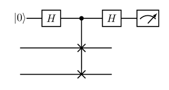
Figure S1: SWAP test.

Now, we regard the local depolarizing channel

$$\Lambda_{p}(\rho)=(1-p)\rho+p/2I_{1}\otimes\mathrm{tr}_{1}(\rho)$$ (S2)

acting on the first qubit with probability $p$ where $\mathrm{tr}_{1}(.)$ is the partial trace over the first qubit. For any pure state $|\psi\rangle$ we find $\gamma(\Lambda_{p}(|\psi\rangle))\geq p-p^{2}/2$.

Let us assume an ensemble of pure states $|\psi\rangle\in\mathcal{E}$. Now, we subject the states to noise, where we define the ensemble of corresponding noisy states $\rho\in\mathcal{E}_{c}$ where $\mathcal{E}_{c}=\{\Lambda_{p}(|\psi\rangle):|\psi\rangle\in\mathcal{E}\}$ with $p=\Omega(n^{-c})$ with $c>0$. For the noisy states we have ${\mathbb{E}}_{\rho\leftarrow\mathcal{E}_{c}}[\gamma(\rho)]=\Omega(n^{-c})$ and thus

$$\left|\underset{\rho\leftarrow\mathcal{E}_{c}}{\mathbb{E}}[\text{Pr}_{\text{SWAP}}(\rho)]-\underset{|\phi\rangle\leftarrow S(\mathcal{H})}{\mathbb{E}}[\text{Pr}_{\text{SWAP}}(|\phi\rangle)]\right|=\Omega(n^{-c})\,.$$ (S3)

We conclude that the SWAP test efficiently distinguishes Haar random states and any ensemble of states affected by $p=\Omega(n^{-c})$ depolarizing noise. Thus, PRSs can have at most $p=\text{negl}(n)$ depolarizing noise.

Next, we consider the case of noisy unitaries. Consider an ensemble of unitaries $U\in\mathcal{G}$. Now, the unitaries are affected by the depolarizing channel Eq. (S2), giving us the ensemble of noisy channels $\Gamma\in\mathcal{G}_{c}$ with $\mathcal{G}_{c}=\{\Lambda_{p}\circ U:U\in\mathcal{G}\}$ where $p=\Omega(n^{-c})$. We now apply the noisy unitaries on a test state $|0\rangle$ and perform the SWAP test. We find

$$\left|\underset{\Gamma\leftarrow\mathcal{G}_{c}}{\mathbb{E}}[\text{Pr}_{\text{SWAP}}(\Gamma(|0\rangle)]-\underset{U\leftarrow\mathcal{U}(\mathcal{H})}{\mathbb{E}}[\text{Pr}_{\text{SWAP}}(U|0\rangle)]\right|=\Omega(n^{-c})\,.$$ (S4)

The SWAP test efficiently distinguishes Haar random unitaries and any unitaries affected by $p=\Omega(n^{-c})$ depolarizing noise. Thus, PRUs can be subject to at most $p=\text{negl}(n)$ depolarizing noise. ∎

SM C:  Proof of inefficient testing of imaginarity for states

Here we show that imaginarity cannot be efficiently tested for states. First, we restate the Theorem 1 the main text:

Theorem S2 (Imaginarity cannot be efficiently tested for states).

Any tester $\mathcal{A}_{\mathcal{I}}$ for imaginarity according to Def. 1 for an $n$-qubit state $|\psi\rangle$ requires $t=\Omega(2^{n/2})$ copies of $|\psi\rangle$ for any $\delta<1-2^{-n+1}$, $\beta<\delta$.

Proof.

Let us first recall Levy’s lemma [68]

Lemma 1 (Levy’s lemma).

Given a function $f:\mathbb{S}(d)\rightarrow\mathbb{R}$ defined on the $d$-dimensional hypersphere $\mathbb{S}(d)$, $\epsilon>0$ and a point $\phi\in\mathbb{S}(d)$ chosen uniformly at random,

$$\mathrm{Pr}(|f(\phi)-\langle f\rangle|\geq\epsilon)\leq 2\exp\left(\frac{-2C(d+1)\epsilon^{2}}{\eta^{2}}\right)$$ (S5)

where $\eta$ is the Lipschitz constant of f, given by $\eta=\mathrm{sup}|\nabla f|$, and $C$ is a positive constant (which can be taken to be $C=(18\pi^{3})^{-1}$.

Due to normalisation, pure states in a $2^{n}$-dimensional Hilbert space can be represented by points on the surface of a ($2\cdot 2^{n}-1$)-dimensional hypersphere $\mathbb{S}(2\cdot 2^{n}-1)$, and hence we can apply Levy’s Lemma to functions of the randomly selected quantum state $|\phi\rangle$ by setting $d=2\cdot 2^{n}-1$.

Next, we bound the Lipschitz constant $\eta$ of imaginarity. For any normalized pure states $|\psi\rangle$, $|\phi\rangle$, we find

$$\eta=\text{max}_{|\psi\rangle,|\phi\rangle}\frac{|\mathcal{I}(|\psi\rangle)-\mathcal{I}(|\phi\rangle)|}{||\psi\rangle-|\phi\rangle|}=2,$$ (S6)

where $||\psi\rangle|$ indicates the Euclidean norm. This can be seen from the following calculation

$$|\mathcal{I}(|\psi\rangle)-\mathcal{I}(|\phi\rangle)| =\frac{1}{4}\left|\||\psi\rangle\langle\psi|-|\psi^{\ast}\rangle\langle\psi^{\ast}|\|_{1}^{2}-\||\phi\rangle\langle\phi|-|\phi^{\ast}\rangle\langle\phi^{\ast}|\|_{1}^{2}\right|$$

$$\leq\frac{1}{4}\||\psi\rangle\langle\psi|-|\phi\rangle\langle\phi|-(|\psi^{\ast}\rangle\langle\psi^{\ast}|-|\phi^{\ast}\rangle\langle\phi^{\ast}|)\|_{1}^{2}$$

$$\leq\frac{1}{4}(\||\psi\rangle\langle\psi|-|\phi\rangle\langle\phi|\|_{1}^{2}+\||\psi^{\ast}\rangle\langle\psi^{\ast}|-|\phi^{\ast}\rangle\langle\phi^{\ast}|\|_{1}^{2})$$

$$=(1-|\langle\psi|\phi\rangle|^{2})\leq||\psi\rangle-|\phi\rangle|^{2}$$ (S7)

where we used the triangle inequalities $|\|x\|-\|y\||\leq\|x-y\|$ and $\|x+y\|\leq\|x\|+\|y\|$. In the last inequality we used

$$1-|\langle\psi|\phi\rangle|^{2} =1-\Re(\langle\psi|\phi\rangle)^{2}-\Im(\langle\psi|\phi\rangle)^{2}\leq 1-\Re(\langle\psi|\phi\rangle)^{2}\leq(1-\Re(\langle\psi|\phi\rangle))(1+\Re(\langle\psi|\phi\rangle))$$

$$\leq 2(1-\Re(\langle\psi|\phi\rangle))=||\psi\rangle-|\phi\rangle|^{2}.$$ (S8)

As we have $||\psi\rangle-|\phi\rangle|\leq 2$, we find $\eta=2$.

From Levy’s lemma and the imaginarity of Haar random states $\mathcal{I}_{\text{Haar}}=\mathbb{E}_{|\psi\rangle\leftarrow S(\mathcal{H})}[\mathcal{I}(|\psi\rangle)]=1-2(2^{n}+1)^{-1}$ (see Eq. (S48)), we have

$$\mathrm{Pr}(|\mathcal{I}(|\psi\rangle)-\mathcal{I}_{\text{Haar}}|\geq\epsilon)\leq 2\exp(-\beta_{0}2^{n}\epsilon^{2}),$$ (S9)

where $\beta_{0}=4C/\eta^{2}=(288\pi^{3})^{-1}\approx 1.8\cdot 10^{-3}$ and $\epsilon>0$. We now drop the absolute value $|.|$ and define $\delta=\mathcal{I}_{\text{Haar}}-\epsilon$ to get

$$\mathrm{Pr}(\mathcal{I}(|\psi\rangle)\leq\delta)\leq 2\exp(-\beta_{0}2^{n}(\mathcal{I}_{\text{Haar}}-\delta)^{2}),$$ (S10)

which is valid for $\delta<\mathcal{I}_{\text{Haar}}$. Thus, the probability that the imaginarity of a randomly sampled state $\mathcal{I}(|\psi\rangle)$ is smaller than any fixed $\delta<\mathcal{I}_{\text{Haar}}(n)=1-2(2^{n}+1)^{-1}$ is super-exponentially small. To simplify the bound we demand $\delta<1-2^{-n+1}<\mathcal{I}_{\text{Haar}}(n)$:

$$P_{\delta}=\underset{|\psi\rangle\leftarrow S(\mathcal{H})}{\text{Pr}}\left[\mathcal{I}(|\psi\rangle)<\delta\right]=2^{-\Omega(2^{n})}\,.$$ (S11)

Let us now define the ensemble $\mathcal{E}_{\mathcal{I}\geq\delta}=\{|\psi\rangle:\mathcal{I}(|\psi\rangle)\geq\delta,|\psi\rangle\in S(\mathcal{H})\}$ of states with imaginarity at least $\delta$ as well as the ensemble $\mathcal{E}_{\mathcal{I}<\delta}=\{|\psi\rangle:\mathcal{I}(|\psi\rangle)<\delta,|\psi\rangle\in S(\mathcal{H})\}$ of states with imaginarity at most $\delta$.

Given the concentration Eq. (S11) and $\delta<1-2^{-n+1}$, the ensemble of states with $\mathcal{I}\geq\delta$ is exponentially close to the ensemble of Haar random states $S(\mathcal{H})$ for any $t$

$$\text{TD}\left(\underset{|\psi\rangle\leftarrow\mathcal{E}_{\mathcal{I}\geq\delta}}{\mathbb{E}}\big{[}|\psi\rangle\langle\psi|^{\otimes t}\big{]},\underset{|\phi\rangle\leftarrow S(\mathcal{H})}{\mathbb{E}}\big{[}|\phi\rangle\langle\phi|^{\otimes t}\big{]}\right)=2^{-\Omega(2^{n})}\,,$$ (S12)

where we have the trace distance $\text{TD}(\rho,\sigma)=\frac{1}{2}\|\rho-\sigma\|_{1}$.

We now prove Eq. (S12) in the following:

$$\text{TD}\left(\underset{|\psi\rangle\leftarrow\mathcal{E}_{\mathcal{I}\geq\delta}}{\mathbb{E}}\big{[}|\psi\rangle\langle\psi|^{\otimes t}\big{]},\underset{|\phi\rangle\leftarrow S(\mathcal{H})}{\mathbb{E}}\big{[}|\phi\rangle\langle\phi|^{\otimes t}\big{]}\right)$$ (S13)

$$=\text{TD}\left((1-P_{\delta})\underset{|\psi\rangle\leftarrow\mathcal{E}_{\mathcal{I}\geq\delta}}{\mathbb{E}}\big{[}|\psi\rangle\langle\psi|^{\otimes t}\big{]}+P_{\delta}\underset{|\psi\rangle\leftarrow\mathcal{E}_{\mathcal{I}<\delta}}{\mathbb{E}}\big{[}|\psi\rangle\langle\psi|^{\otimes t}\big{]}\right.$$

$$\left.\quad-P_{\delta}(\underset{|\psi\rangle\leftarrow\mathcal{E}_{\mathcal{I}<\delta}}{\mathbb{E}}\big{[}|\psi\rangle\langle\psi|^{\otimes t}\big{]}-\underset{|\psi\rangle\leftarrow\mathcal{E}_{\mathcal{I}\geq\delta}}{\mathbb{E}}\big{[}|\psi\rangle\langle\psi|^{\otimes t}\big{]}),\underset{|\phi\rangle\leftarrow S(\mathcal{H})}{\mathbb{E}}\big{[}|\phi\rangle\langle\phi|^{\otimes t}\big{]}\right)$$

$$=\text{TD}\left(\underset{|\phi\rangle\leftarrow S(\mathcal{H})}{\mathbb{E}}\big{[}|\phi\rangle\langle\phi|^{\otimes t}\big{]}-P_{\delta}(\underset{|\psi\rangle\leftarrow\mathcal{E}_{\mathcal{I}<\delta}}{\mathbb{E}}\big{[}|\psi\rangle\langle\psi|^{\otimes t}\big{]}-\underset{|\psi\rangle\leftarrow\mathcal{E}_{\mathcal{I}\geq\delta}}{\mathbb{E}}\big{[}|\psi\rangle\langle\psi|^{\otimes t}\big{]}),\underset{|\phi\rangle\leftarrow S(\mathcal{H})}{\mathbb{E}}\big{[}|\phi\rangle\langle\phi|^{\otimes t}\big{]}\right)$$

$$=P_{\delta}\text{TD}\left(\underset{|\psi\rangle\leftarrow\mathcal{E}_{\mathcal{I}<\delta}}{\mathbb{E}}\big{[}|\psi\rangle\langle\psi|^{\otimes t}\big{]},\underset{|\psi\rangle\leftarrow\mathcal{E}_{\mathcal{I}\geq\delta}}{\mathbb{E}}\big{[}|\psi\rangle\langle\psi|^{\otimes t}\big{]}\right)=2^{-\Omega(2^{n})},$$

where in the second step we used

$$(1-P_{\delta})\underset{|\psi\rangle\leftarrow\mathcal{E}_{\mathcal{I}\geq\delta}}{\mathbb{E}}\big{[}|\psi\rangle\langle\psi|^{\otimes t}\big{]}+P_{\delta}\underset{|\psi\rangle\leftarrow\mathcal{E}_{\mathcal{I}<\delta}}{\mathbb{E}}\big{[}|\psi\rangle\langle\psi|^{\otimes t}\big{]}=\underset{|\phi\rangle\leftarrow S(\mathcal{H})}{\mathbb{E}}\big{[}|\phi\rangle\langle\phi|^{\otimes t}\big{]}$$ (S14)

and in the last step $\text{TD}(\rho,\sigma)\leq 1$ for any valid quantum states $\rho$, $\sigma$.

Next, we recall the $K$-subset phase states introduced in Ref. [13]

$$|\psi_{S,f}\rangle=\frac{1}{|S|}\sum_{x\in S}(-1)^{f(x)}|x\rangle,$$ (S15)

where $S$ is a set of binary strings $\{0,1\}^{n}$ with exactly $K=|S|$ elements and $f:\{0,1\}^{n}\to\{0,1\}$ a binary phase function. Let us also define the set of all $K$-subset phase states $\mathcal{E}_{\text{p}}^{K}=\{|\psi_{S,f}\rangle\}_{S\,\text{with}\,|S|=K,\,f}$ which contains the states $|\psi_{S,f}\rangle$ with all binary phase functions $f$ and all $S$ with $K=|S|$.

The ensemble $\mathcal{E}_{\text{p}}$ of phase states Eq. (S15) has been shown to be statistically close to the ensemble of Haar random states (Theorem 2.1 of Ref. [13])

$$\text{TD}\left(\underset{|\psi\rangle\leftarrow\mathcal{E}_{\text{p}}^{K}}{\mathbb{E}}\big{[}|\psi\rangle\langle\psi|^{\otimes t}\big{]},\underset{|\phi\rangle\leftarrow S(\mathcal{H})}{\mathbb{E}}\big{[}|\phi\rangle\langle\phi|^{\otimes t}\big{]}\right)=O\left(\frac{t^{2}}{K}\right)\,.$$ (S16)

It follows from the triangle inequality $\text{TD}(\rho,\sigma)\leq\text{TD}(\rho,\theta)+\text{TD}(\theta,\sigma)$ applied on Eq. (S12) and Eq. (S16) that

$$\text{TD}\left(\underset{|\psi\rangle\leftarrow\mathcal{E}_{\text{p}}^{K}}{\mathbb{E}}\big{[}|\psi\rangle\langle\psi|^{\otimes t}\big{]},\underset{|\phi\rangle\leftarrow\mathcal{E}_{\mathcal{I}\geq\delta}}{\mathbb{E}}\big{[}|\phi\rangle\langle\phi|^{\otimes t}\big{]}\right)=O\left(\frac{t^{2}}{K}\right)\,.$$ (S17)

Eq. (S17) implies that the ensemble of phase states and the ensemble of states with imaginarity $\mathcal{I}(|\psi\rangle)\geq\delta$ (where $\delta<1-2^{-n+1}$) are exponentially close in trace-distance unless $t=\Omega(\sqrt{K})$.

Two ensembles can be distinguished only if they are sufficiently far in TD distance. In particular, for any state discrimination protocol between two ensembles $\rho$, $\sigma$, the maximal possible discrimination probability is given by the Helstrom bound [69]

$$P_{\text{discr}}(\rho,\sigma)=\frac{1}{2}+\text{TD}(\rho,\sigma)\,.$$ (S18)

In particular, any algorithm trying to distinguish two ensembles with $P_{\text{discr}}\geq 2/3$ requires at least $\text{TD}(\rho,\sigma)\geq 1/6$.

We now consider the case $K=2^{n}$, i.e. subset phase states with support on all $2^{n}$ computational basis states. To achieve $P_{\text{discr}}=\Omega(1)$ between $t$ copies of $\mathcal{E}_{\text{p}}^{2^{n}}$ and $\mathcal{E}_{\mathcal{I}\geq\delta}$, we require $t=\Omega(2^{n/2})$ for $\delta\leq 1-2^{-n+1}$. Thus, testing imaginarity also requires $t=\Omega(2^{n/2})$ copies. ∎

Note that for the proof we used the subset phase states with $\mathcal{I}=0$, and thus our result extends for any state with larger imaginarity for any threshold $0\leq\beta<\delta$. Note that $\delta\leq 1-2^{-n+1}$ converges to maximal imaginarity for large $n$, i.e. testing imaginarity is inefficient for any value of imaginarity in an asymptotic sense.

SM D:  Inefficient algorithm to measure imaginarity of states

Now, we discuss a scheme to measure imaginarity for pure states. In particular, we have

$$\mathcal{I}(|\psi\rangle)=1-2^{n}\langle\psi|^{\otimes 2}(|\Phi\rangle\langle\Phi|)|\psi\rangle^{\otimes 2}\,,$$ (S19)

where $|\Phi\rangle=2^{-n/2}\sum_{k=0}^{2^{n}-1}|k\rangle|k\rangle$ is the maximally entangled state. To measure imaginarity, one computes the probability of the projector $|\Phi\rangle\langle\Phi|$ for two copies of state $|\psi\rangle^{\otimes 2}$. Using the Ricochet property S24, it is easy to see for $|\psi\rangle=U|0\rangle$ with arbitrary unitary $U$ via

$$\langle\psi|^{\otimes 2}|\Phi\rangle\langle\Phi||\psi\rangle^{\otimes 2}=\langle 0|^{\otimes 2}U^{\dagger}\otimes U^{\dagger}|\Phi\rangle\langle\Phi|U\otimes U|0\rangle^{\otimes 2}$$

$$= \langle 0|^{\otimes 2}U^{\dagger}{U^{\text{T}}}^{\dagger}\otimes I|\Phi\rangle\langle\Phi|U^{\text{T}}U\otimes I|0\rangle^{\otimes 2}$$

$$= 2^{-n}\langle 0|{U^{\dagger}U^{\text{T}}}^{\dagger}|0\rangle\langle 0|U^{\text{T}}U|0\rangle=2^{-n}|\langle\psi|\psi^{*}\rangle|^{2},$$

where we made use of Eq. (S24) and ${U^{\text{T}}}^{\dagger}=U^{\ast}$. This completes the proof of Eq. (S19).

We measure the observable $2^{n}|\Phi\rangle\langle\Phi|$ which has two possible outcomes with eigenvalues $\lambda_{1}=2^{n}$ and $\lambda_{2}=0$, occurring with probability $q_{1}=\langle\psi|^{\otimes 2}|\Phi\rangle\langle\Phi||\psi\rangle^{\otimes 2}$ probability and $q_{2}=1-q_{1}$. The range of outcomes is $\Delta\lambda=2^{n}$, which using Hoeffding’s inequality Eq. (S27) gives us the upper bound of measurements $M=O(4^{n})$.

In practice, the bound is loose and one can achieve better performance of $M\sim 2^{n}$ as we argue in the following. Measuring $\mathcal{I}$ is a binomial process, where the standard deviation $\text{std}(\mathcal{I})$ is given by

$$\text{std}(\mathcal{I})=\left(\frac{q_{1}q_{2}}{M}\right)^{1/2}\approx M^{-1/2}2^{n/2}\,,$$ (S20)

where we used $\langle\psi|^{\otimes 2}|\Phi\rangle\langle\Phi||\psi\rangle^{\otimes 2}\approx 2^{-n}$. From this we expect to require $M\sim 2^{n}\text{std}(\mathcal{I})^{-2}$ measurements.

We investigate the number of measurements $M$ needed to estimate $\mathcal{I}$ for a randomly chosen real state in Fig. S2. We generate a random real state by sampling a Haar random unitary $U$, and preparing the state $c(U_{\text{Haar}}+U_{\text{Haar}}^{*})|0\rangle$, where $c$ is an appropriate normalization factor. In Fig. S2a, we show that the measurement error $\Delta\mathcal{I}=|\hat{\mathcal{I}}-\mathcal{I}|$ scales as $\Delta\mathcal{I}\sim M^{-1/2}$. In Fig. S2b, we find that $\Delta\mathcal{I}\sim 2^{0.58n}$. Both results together confirm $M\sim 2^{n}$ for constant $\Delta\mathcal{I}$. Note that the algorithm is likely not optimal as it does not saturate the lower bound of Theorem 2.

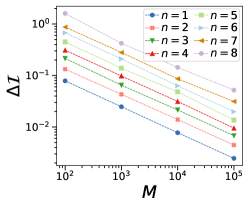
 a  b

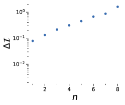
Figure S2: Measurement error $\Delta\mathcal{I}=|\hat{\mathcal{I}}-\mathcal{I}|$ for a random real state as a function of measurements $M$ and qubit number $n$. a) Error $\Delta\mathcal{I}$ against $M$, where we find $\Delta\mathcal{I}\propto M^{-1/2}$. b) $\Delta\mathcal{I}$ against $n$. Dashed line is fit with $\Delta\mathcal{I}\propto 2^{0.58n}$.

SM E:  Efficient measurement of imaginarity for stabilizer states

Claim S1 (Imaginarity of stabilizer states can be measured efficiently).

Given a stabilizer state $|\psi\rangle\in\mathrm{STAB}$, imaginarity can be computed via

$$\mathcal{I}(|\psi\rangle)\equiv\mathcal{I}_{\mathrm{STAB}}(|\psi\rangle)=1-2^{-n}\sum_{\sigma\in\mathcal{P}}|\langle\psi|\sigma|\psi^{*}\rangle|^{2}|\langle\psi|\sigma|\psi\rangle|^{2},$$ (S21)

where $\mathcal{P}$ is the set of all Pauli strings with phase $+1$. $\mathcal{I}_{\mathrm{STAB}}$ can be efficiently measured within additive precision $\delta$ with a failure probability $\nu$ using at most $t=O(\delta^{-2}\log(1/\nu))$ copies.

Proof.

We denote the Pauli matrices by $\sigma_{00}=I_{2}$, $\sigma_{01}=\sigma^{x}$, $\sigma_{10}=\sigma^{z}$ and $\sigma_{11}=\sigma^{y}$. We define the set of all $4^{n}$ Pauli strings $\mathcal{P}=\{\sigma_{\boldsymbol{r}}\}_{\boldsymbol{r}}$ with $+1$ phase by $N$-qubit tensor products of Pauli matrices given by $\sigma_{\boldsymbol{r}}=\bigotimes_{j=1}^{n}\sigma_{\boldsymbol{r}_{2j-1}\boldsymbol{r}_{2j}}$ with $\boldsymbol{r}\in\{0,1\}^{2n}$.

 

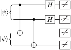
Figure S3: Bell measurement for state $|\psi\rangle$.

A stabilizer state $|\psi_{\mathrm{STAB}}\rangle$ is defined by a commuting subgroup $G$ of $\left|G\right|=2^{n}$ Pauli strings $\sigma$. We have $\langle\psi_{\mathrm{STAB}}|\sigma|\psi_{\mathrm{STAB}}\rangle=\pm 1$ for $\sigma\in G$ and $\langle\psi_{\mathrm{STAB}}|\sigma^{\prime}|\psi_{\mathrm{STAB}}\rangle=0$ for $\sigma^{\prime}\notin G$ [55].

Input :  $4M$ copies of $|\psi\rangle$

Output : $\mathcal{I}_{\mathrm{STAB}}$

1

2$b=0$

3 for $\ell=1,\dots,M$ do

4       Prepare $|\eta\rangle=U_{\text{Bell}}^{\otimes n}|\psi\rangle|\psi\rangle$

5      Sample $\boldsymbol{r}\sim|\langle\boldsymbol{r}|\eta\rangle|^{2}$

6       for $k=1,2$ do

7             Prepare $|\psi\rangle$ and measure in eigenbasis of Paulistring $\sigma_{\boldsymbol{r}}$ to get eigenvalue $\lambda_{k}\in\{+1,-1\}$

8       end for

9      $b=b+\lambda_{1}\lambda_{2}$

10 end for

11$\mathcal{I}_{\mathrm{STAB}}=1-b/M$

Algorithm 1 Imaginarity of stabilizer states

We now propose Algorithm 1 to efficiently measure the imaginarity of stabilizer states. We recall the Bell transformation $U_{\text{Bell}}=(H\otimes I_{1})\text{CNOT}$ (see also Fig. S3), where $H=\frac{1}{\sqrt{2}}(\sigma^{x}+\sigma^{z})$ is the Hadamard gate, and $\text{CNOT}=\exp(i\frac{\pi}{4}(I_{1}-\sigma^{z})\otimes(I_{1}-\sigma^{x}))$. We apply the Bell transformation on two copies $|\psi\rangle\otimes|\psi\rangle$ and measure in the computational basis. The outcome $\boldsymbol{r}$ corresponding to computational basis state $|\boldsymbol{r}\rangle$ is sampled with a probability [70]

$$P(\boldsymbol{r})=\langle\psi|\langle\psi|{U_{\text{Bell}}^{\otimes n}}^{\dagger}|\boldsymbol{r}\rangle\langle\boldsymbol{r}|U_{\text{Bell}}^{\otimes n}|\psi\rangle|\psi\rangle=2^{-n}|\langle\psi|\sigma_{\boldsymbol{r}}|\psi^{*}\rangle|^{2}\,.$$ (S22)

Using a combination of Bell measurements and Pauli measurements [44], we propose to measure the imaginarity of stabilizer states via

$$\mathcal{I}_{\mathrm{STAB}}(|\psi\rangle):=1-\underset{\boldsymbol{r}\sim P(\boldsymbol{r})}{\mathbb{E}}[|\langle\psi|\sigma_{\boldsymbol{r}}|\psi\rangle|^{2}].$$ (S23)

In particular, given a stabilizer state $|\psi\rangle\in\mathrm{STAB}$ we find

$$\mathcal{I}_{\mathrm{STAB}}(|\psi\rangle) =1-2^{-n}\sum_{\sigma\in\mathcal{P}}|\langle\psi|\sigma|\psi^{*}\rangle|^{2}|\langle\psi|\sigma|\psi\rangle|^{2}$$

$$=1-2^{-n}\sum_{\sigma\in G}|\langle\psi|\sigma|\psi^{*}\rangle|^{2}=1-|\langle\psi|\psi^{*}\rangle|^{2}\equiv\mathcal{I}(|\psi\rangle)\,,$$

where in the second line we used $\sigma|\psi\rangle=\pm|\psi\rangle$ for $|\psi\rangle\in\mathrm{STAB}$ with corresponding $\sigma\in G(|\psi\rangle)$, and $\langle\psi|\sigma|\psi\rangle=0$ for $\sigma\notin G(|\psi\rangle)$.

Note that non-real stabilizer states $|\psi_{\mathrm{STAB}}^{I}\rangle\notin\mathbb{R}^{2^{n}}$ are always maximally imaginary, i.e. $\mathcal{I}(|\psi_{\mathrm{STAB}}^{I}\rangle)=1$ and $|\langle\psi_{\mathrm{STAB}}^{I}|{\psi^{I}_{\mathrm{STAB}}}^{*}\rangle|^{2}=0$. This can be easily seen from the fact that $|\langle\psi_{\mathrm{STAB}}|\sigma|\psi_{\mathrm{STAB}}\rangle|^{2}\in\{0,1\}$ and $|\psi^{*}_{\mathrm{STAB}}\rangle=\bigotimes_{k=1}^{n}\sigma_{z}^{\alpha_{k}}|\psi_{\mathrm{STAB}}\rangle$ with some $\alpha_{k}\in\{0,1\}$ [70]. Thus, it follows $|\langle\psi_{\mathrm{STAB}}|\psi^{*}_{\mathrm{STAB}}\rangle|^{2}=|\langle\psi_{\mathrm{STAB}}|\bigotimes_{k=1}^{n}\sigma_{z}^{\alpha_{k}}|\psi_{\mathrm{STAB}}\rangle|^{2}$. For any imaginary stabilizer, we necessarily have $|\langle\psi_{\mathrm{STAB}}^{I}|{\psi^{I}_{\mathrm{STAB}}}^{*}\rangle|^{2}<1$, and therefore $|\langle\psi_{\mathrm{STAB}}^{I}|{\psi^{I}_{\mathrm{STAB}}}^{*}\rangle|^{2}=0$.

Each repetition of the algorithm yields outcome $\lambda_{1}=-1$ or $\lambda_{2}=1$ with range of outcomes $\Delta\lambda=2$. Due to Hoeffding’s inequality Eq. (S27), the number of repetitions $M$ needed to reach an accuracy $\delta$ with a failure probability $\nu$ for Algorithm 1 is bounded by $M=O(\delta^{-2}\log(2/\nu))$. As real stabilizer states have $\mathcal{I}=0$, while imaginary stabilizer states must have $\mathcal{I}=1$, this directly implies that one can efficiently distinguish real and complex-valued stabilizer states with $t=O(1)$ copies of $|\psi\rangle$. ∎

We also propose Eq. (S23) as an efficient witness of non-imaginarity, which we define in analogy to entanglement witnesses [71]. When a non-imaginarity witness is zero, the state must be real. When the witness is greater than zero, then the state may be either real or imaginary.  Eq. (S23) fulfills this condition as it is zero only when for real stabilizer states, and greater than zero for all other states [44].

SM F:  Efficient measurement of imaginarity for unitaries

Here, we show that measuring imaginarity $\mathcal{I}_{\text{p}}(U)$ of an $n$-qubit unitary $U$ is efficient. Imaginarity for unitaries can be defined via its Choi-state

$$\mathcal{I}_{\text{p}}(U) \equiv\mathcal{I}(U\otimes I|\Phi\rangle)=1-|\langle\Phi|(U^{\dagger}\otimes I)(U^{*}\otimes I)|\Phi\rangle|^{2}=1-4^{-n}\left|\mathrm{tr}(U^{\dagger}U^{\ast})\right|^{2}\,.$$

Let us restate the Claim to be proven:

Claim S2 (Imaginarity of unitaries can be measured efficiently).

Measuring $\mathcal{I}_{\text{p}}(U)$ within additive precision $\delta$ with a failure probability $\nu$ requires at most $t=O(\delta^{-2}\log(1/\nu))$ copies.

Proof.

First, we define the maximally entangled state $|\Phi\rangle=2^{-n/2}\sum_{k=0}^{2^{n}-1}|k\rangle|k\rangle$ over $2n$ qubits. Then, we prepare the state $|\eta\rangle=U\otimes U|\Phi\rangle$. We then measure the expectation value $P_{\Phi}(U)=|\langle\Phi|\eta\rangle|^{2}$ of the projector $|\Phi\rangle\langle\Phi|$

$$P_{\Phi}(U) =4^{-n}\Big{|}\sum_{q,k}\langle q|\langle q|U\otimes U|k\rangle|k\rangle\Big{|}^{2}=4^{-n}\Big{|}\sum_{q,k}\langle q|\langle q|UU^{T}\otimes I|k\rangle|k\rangle\Big{|}^{2}=4^{-n}\Big{|}\sum_{k}\langle k|UU^{T}|k\rangle\Big{|}^{2}$$

$$=4^{-n}\left|\mathrm{tr}(UU^{T})\right|^{2}=4^{-n}\left|\mathrm{tr}(U^{\dagger}U^{\ast})\right|^{2},$$

where we used the Ricochet property [72]

$$\sum_{k=0}^{2^{n}-1}A\otimes I_{n}|k\rangle|k\rangle=\sum_{k=0}^{2^{n}-1}I_{n}\otimes A^{T}|k\rangle|k\rangle\,$$ (S24)

for any $n$-qubit operator $A$. Thus, we can write imaginarity as

$$\mathcal{I}_{\text{p}}(U)=1-P_{\Phi}(U)\,.$$ (S25)

$P_{\Phi}(U)$ can be measured efficiently by sampling in the Bell basis and measuring the probability of sampling $|\Phi\rangle$. We upper bound the required number of measurements $M$ with Hoeffding’s inequality

$$\text{Pr}(|\hat{\mathcal{I}}-\mathcal{I}|\geq\delta)=\nu\leq 2\exp\left(-\frac{2\delta^{2}M}{\Delta\lambda^{2}}\right)\,,$$ (S26)

where $\hat{\mathcal{I}}_{\text{p}}$ is the estimation of exact value $\mathcal{I}_{\text{p}}$ from $M$ Bell measurements, $\delta$ is the allowed error, $\Delta\lambda=1$ is the range of possible measurement outcomes and $\nu$ is the failure probability of getting an error larger than $\delta$. By inverting we find

$$M\leq\frac{\Delta\lambda}{2\delta^{2}}\log\left(\frac{2}{\nu}\right)=\frac{1}{2\delta^{2}}\log\left(\frac{2}{\nu}\right)\,,$$ (S27)

To achieve an error of at most $\delta$ with a probability of failure $\nu$, we require at most $M=O(\delta^{-2}\log(\nu^{-1}))$ measurements and $2M$ instances of $U$. The classical post-processing time scales as $O(n)$, which is asymptotically optimal.

∎

SM G:  PRUs require imaginarity

Theorem S3.

PRUs require imaginarity $\mathcal{I}_{\text{p}}=1-\mathrm{negl}(n)$.

Proof.

We measure $P_{|\Phi\rangle}=1-\mathcal{I}_{\text{p}}(U)$ which was introduced in the proof for Claim 2. We can interpret the measurement as a tester: We prepare $U\otimes U|\Phi\rangle$ and measure the projection onto $|\Phi\rangle\langle\Phi|$. The tester accepts when we get $|\Phi\rangle$ as outcome, else the tester rejects.

First, we consider a set of $n$-qubit unitaries $\mathcal{E}_{c}$ with imaginarity $\mathbb{E}_{U\leftarrow\mathcal{E}_{c}}[\mathcal{I}_{\text{p}}(U)]=1-\Omega(n^{-c})$. For the acceptance probability of the test, we find $\mathbb{E}_{U\leftarrow\mathcal{E}_{c}}[P_{\Phi}(U)]=\Omega(n^{-c})$.

In contrast, for Haar random unitaries we find $\mathbb{E}_{U\leftarrow\mathcal{U}(\mathcal{H})}[P_{\Phi}(U)]=2(2^{n}(2^{n}+1))^{-1}=O(4^{-n})$ (SM 2).

Thus, one can efficiently distinguish Haar random unitaries from $\mathcal{E}_{c}$, which places a lower bound the imaginarity of PRUs as $\mathcal{I}_{\text{p}}=1-\mathrm{negl}(n)$. ∎

SM H:  Coherence testing for states

We now show the limits on coherence testing for states. First, we recall the definition of relative entropy of coherence for pure states $|\psi\rangle$

$$\mathcal{C}(|\psi\rangle)=-\sum_{k}{|c_{k}|^{2}}\ln(|c_{k}|^{2}).$$ (S28)

Next, we restate the theorem of the main text:

Theorem S4 (Lower bound on coherence testing for states).

Any tester $\mathcal{A}_{\mathcal{C}}$ for relative entropy of coherence according to Def. 1 for an $n$-qubit state $|\psi\rangle$ requires $t=\Omega(2^{\beta/2})$ for any $\delta<n\ln(2)-1$ and $\beta<\delta$.

Proof.

First, we note that Haar random states concentrate around a large, but non-maximal value of coherence [56]. The coherence of $n$-qubit Haar random states is on average

$$\mathcal{C}_{\text{Haar}}=\underset{|\phi\rangle\leftarrow S(\mathcal{H})}{\mathbb{E}}[\mathcal{C}(|\phi\rangle)]=\sum_{k=2}^{2^{n}}\frac{1}{k}\,,$$ (S29)

where for $n\gg 1$ we have $\mathcal{C}_{\text{Haar}}=\gamma_{\text{EM}}-1+n\ln(2)+O(2^{-n})$, where $\gamma_{\text{EM}}=0.57721$ is the Euler–Mascheroni constant. Haar random states concentrate around their average value with exponentially high probability [56]

$$\mathrm{Pr}(|\mathcal{C}(|\psi\rangle)-\mathcal{C}_{\text{Haar}}|\geq\epsilon)\leq 2\exp\left(-\frac{2^{n}\epsilon^{2}}{36\pi^{3}\ln(2)(n\ln 2)^{2}}\right).$$ (S30)

We relax $\delta\leq n\ln(2)-1\leq n\ln(2)-1+\gamma_{\text{EM}}$. We thus find for any $\delta\leq n\ln(2)-1$

$$\mathrm{Pr}(\mathcal{C}(|\psi\rangle)<\delta)\leq 2^{-\Omega(2^{n})}\,.$$ (S31)

We now define the ensemble $\mathcal{E}_{\mathcal{C}\geq\delta}$ of all states with a relative entropy of coherence greater $\delta$.

Given the concentration Eq. (S31), the ensemble $\mathcal{E}_{\mathcal{C}\geq\delta}$ is exponentially close to the ensemble $S(\mathcal{H})$ of random states for any $t$

$$\text{TD}\left(\underset{|\psi\rangle\leftarrow\mathcal{E}_{\mathcal{C}\geq\delta}}{\mathbb{E}}\big{[}|\psi\rangle\langle\psi|^{\otimes t}\big{]},\underset{|\phi\rangle\leftarrow S(\mathcal{H})}{\mathbb{E}}\big{[}|\phi\rangle\langle\phi|^{\otimes t}\big{]}\right)=2^{-\Omega(2^{n})}\,,$$ (S32)

where the proof follows the one for imaginarity given in Eq. (S13). Further, we recall that Haar random states are close to $K$-subset phase states Eq. (S16). We recall the triangle inequality $\text{TD}(\rho,\sigma)\leq\text{TD}(\rho,\theta)+\text{TD}(\theta,\sigma)$ and apply it on Eq. (S32) and Eq. (S16) to get for any $\delta\leq n\ln(2)-1$

$$\text{TD}\left(\underset{|\psi\rangle\leftarrow\mathcal{E}_{\text{p}}^{K}}{\mathbb{E}}\big{[}|\psi\rangle\langle\psi|^{\otimes t}\big{]},\underset{|\phi\rangle\leftarrow\mathcal{E}_{\mathcal{C}\geq\delta}}{\mathbb{E}}\big{[}|\phi\rangle\langle\phi|^{\otimes t}\big{]}\right)\leq O\left(\frac{t^{2}}{K}\right).$$ (S33)

For any $K$-subset phase state $|\psi\rangle\in\mathcal{E}_{\text{p}}^{K}$, we have $\mathcal{C}(|\psi\rangle)=\ln(K)$. With Eq. (S33) and Helstrom bound Eq. (S18), we require $t=\Omega(\sqrt{K})=\Omega(2^{\mathcal{C}/2})$ copies to distinguish $K$-subset phase states from states drawn from the ensemble of states with $\mathcal{C}\geq\delta$. ∎

Next, we show that one can efficiently test for coherence as defined by the Hilbert-Schmidt norm [26]

$$\mathcal{C}_{2}(|\psi\rangle)=1-\sum_{k}{|c_{k}|^{4}}\,,$$ (S34)

where $|\psi\rangle=\sum_{k}c_{k}|k\rangle$ with amplitudes $c_{k}$ [26]. We have $0\leq\mathcal{C}_{2}\leq 1-2^{-n}$. Further, $\mathcal{C}_{2}(|\psi\rangle)=0$ if and only if $\mathcal{C}(|\psi\rangle)=0$.

For this measure of coherence, we have an efficient measurement protocol:

Proposition 1 (Efficient measurement of coherence).

Measuring $\mathcal{C}_{2}(|\psi\rangle)$ within additive precision $\delta$ with a failure probability $\nu$ requires at most $t=O(\delta^{-2}\log(1/\nu))$ copies.

Proof.

$\mathcal{C}_{2}$ is measured efficiently with the projector $\Pi_{\mathcal{C}}=\bigotimes_{k=1}^{n}(|00\rangle\langle 00|+|11\rangle\langle 11|)$

$$\mathcal{C}_{2}(|\psi\rangle)=1-\langle\psi|^{\otimes 2}\Pi_{\mathcal{C}}|\psi\rangle^{\otimes 2}\,.$$ (S35)

The projector $\Pi_{\mathcal{C}}$ has possible eigenvalues $\lambda=0$ or $\lambda=1$, with eigenvalue range $\Delta\lambda=1$. Using Hoeffding’s inequality Eq. (S27), we can upper bound the number of copies $M=O(1)$ for reaching a fixed precision. ∎

Now, as stated in the main text, we prove that PRSs require sufficient relative entropy of coherence:

Claim S3.

PRSs require $\mathcal{C}=\omega(\log(n))$ coherence.

Proof.

We show that one can efficiently distinguish Haar random states and states with $\mathcal{C}=O(\log(n))$.

We now use the following tester: We measure the projector $\Pi_{\mathcal{C}}$ on the state $|\psi\rangle^{\otimes 2}$ from Eq. (S35). We say the tester accepts when the projector $\Pi_{\mathcal{C}}$ is successful, else we say the tester rejects the state.

Lets regard an ensemble $\mathcal{E}_{c}$ of states which have on average $\mathbb{E}_{|\psi\rangle\leftarrow\mathcal{E}_{c}}[\mathcal{C}_{2}(|\psi\rangle)]=1-\Omega(n^{-c})$. We have acceptance probability $\mathbb{E}_{|\psi\rangle\leftarrow\mathcal{E}_{c}}[\langle\psi|^{\otimes 2}\Pi_{\mathcal{C}}|\psi\rangle^{\otimes 2}]=\Omega(n^{-c})$.

For Haar random states, we can calculate the average coherence by standard Haar integration

$$\mathbb{E}_{|\phi\rangle\leftarrow S(\mathcal{H})}[\mathcal{C}_{2}(|\phi\rangle)] =\int_{U}\mathcal{C}_{2}(U|0\rangle)\text{d}U=1-\sum_{k}\int_{U}|\langle k|U|0\rangle|^{4}\text{d}U=1-2^{n}\int_{U}|\langle 0|U|0\rangle|^{4}\text{d}U$$

$$=1-2^{n}\int_{U}\mathrm{tr}(U^{\dagger}|0\rangle\langle 0|U|0\rangle\langle 0|U^{\dagger}|0\rangle\langle 0|U|0\rangle\langle 0|)\text{d}U=1-\frac{2}{2^{n}+1}$$

where at the third equality we used the left invariance of Haar random unitaries and in the last step a standard identity for Haar random integrals. We thus find $\mathbb{E}_{|\phi\rangle\leftarrow S(\mathcal{H})}[\mathcal{C}_{2}(|\phi\rangle)]=1-O(2^{-n})$ and thus $\mathbb{E}_{|\psi\rangle\leftarrow S(\mathcal{H})}[\langle\psi|^{\otimes 2}\Pi_{\mathcal{C}}|\psi\rangle^{\otimes 2}]=O(2^{-n})$.

By repeating the testing a polynomial number of times, we can distinguish Haar random states and states drawn from $\mathcal{E}_{c}$ with $\Omega(1)$ probability.

As we can efficiently distinguish Haar random states and states with $\mathcal{C}_{2}=1-\Omega(n^{-c})$, PRSs must have $\mathcal{C}_{2}=1-2^{-\omega(\log(n))}$. From Jensen’s inequality, we have $\mathcal{C}(|\psi\rangle)\geq-\ln(1-\mathcal{C}_{2}(|\psi\rangle))$. Thus, PRSs have $\mathcal{C}(|\psi\rangle)=\omega(\log(n))$.

∎

SM I:  PRUs and coherence power

We now show that PRUs require a sufficient amount of coherence. First, we restate the theorem from the main text:

Theorem S5.

PRUs require $\mathcal{C}_{\text{p}}=\omega(\log(n))$ relative entropy of coherence power.

Proof.

Let us define the following efficient testing algorithm for coherence power of an $n$-qubit unitary $U$: We efficiently prepare the $2n$-qubit state

$$\chi(U)=(\mathcal{D}_{n}U\mathcal{D}_{n}U)^{\otimes 2}(|\Phi\rangle\langle\Phi|),$$ (S36)

where $\mathcal{D}_{n}(\rho)=\sum_{k=0}^{2^{n}-1}|k\rangle\langle k|\langle k|\rho|k\rangle$ is the $n$-qubit coherence-destroying channel. $\mathcal{D}_{n}$ can be efficiently implemented by measuring the state $\rho$ in the computational basis. Next, we perform the SWAP test between the bipartition of $\chi(U)$. The SWAP test is shown in Fig. S1. We say the SWAP test accepts when the measurement returns $0$ which occurs with probability $\text{Pr}_{\text{SWAP}}(U)=(1+\text{tr}(S\chi(U)))/2$ where $S=\sum_{k\ell}=|k\ell\rangle\langle\ell k|$ is the SWAP operator. This measurement gives us the coherence power via [29]

$$\text{tr}(S\chi(U))=2^{-n}\sum_{k,\ell}|\langle k|U|\ell\rangle|^{4}\,.$$ (S37)

Let us now consider a set of unitaries $\mathcal{E}_{c}$ with on average $\mathbb{E}_{U\leftarrow\mathcal{E}_{c}}[2^{-n}\sum_{k,\ell}|\langle k|U|\ell\rangle|^{4}]=\Omega(n^{-c})$ with $c>0$. The SWAP test accepts with probability $\mathbb{E}_{U\leftarrow\mathcal{E}_{c}}[\text{Pr}_{\text{SWAP}}(U)]=\frac{1}{2}+\Omega(n^{-c})$. For Haar random states, we have $\mathbb{E}_{U\leftarrow\mathcal{U}(\mathcal{H})}[2^{-n}\sum_{k,\ell}|\langle k|U|\ell\rangle|^{4}]=2^{-n+1}(1+2^{-n})^{-1}$ [29] and thus $\mathbb{E}_{U\leftarrow\mathcal{U}(\mathcal{H})}[\text{Pr}_{\text{SWAP}}(U)]=\frac{1}{2}+O(2^{-n})$. By repeating the test a polynomial number of times, we can distinguish Haar random unitaries and states drawn from $\mathcal{E}_{c}$ with $\Omega(1)$ probability.

Thus, an ensemble of PRUs $\mathcal{E}_{\text{PR}}$ must have $\mathbb{E}_{U\leftarrow{\mathcal{E}_{\text{PR}}}}[2^{-n}\sum_{k,\ell}|\langle k|U|\ell\rangle|^{4}]=2^{-\omega(\log(n))}$. From Jensen’s inequality, we have $\mathbb{E}_{U\leftarrow{\mathcal{E}_{\text{PR}}}}[-\ln(2^{-n}\sum_{k,\ell}|\langle k|U|\ell\rangle|^{4})]=\omega(\log(n))$.

Now, note that we have $2^{-n}\sum_{k,\ell}|\langle k|U|\ell\rangle|^{2}=1$, where $\xi_{k\ell}(U)=2^{-n}|\langle k|U|\ell\rangle|^{2}$ can be thought of as a probability distribution. From the well-known inequalities of Rényi entropies, we have

$$\ln(2^{-n}\text{card}(U))\geq-2^{-n}\sum_{k,\ell}|\langle k|U|\ell\rangle|^{2}\ln(|\langle k|U|\ell\rangle|^{2})\geq-\ln(2^{-n}\sum_{k,\ell}|\langle k|U|\ell\rangle|^{4})\,.$$ (S38)

Finally, we use $-2^{-n}\sum_{k,\ell}|\langle k|U|\ell\rangle|^{2}\ln(|\langle k|U|\ell\rangle|^{2})\geq-\ln(2^{-n}\sum_{k,\ell}|\langle k|U|\ell\rangle|^{4})$ to get $\mathbb{E}_{U\leftarrow{\mathcal{E}_{\text{PR}}}}[\mathcal{C}(U)]=\omega(\log(n))$. ∎

SM J:  Imaginarity for rebits

While rebits are by definition real, we can define imaginarity such that it matches the definition of qubits.

We have the $n$-qubit qubit state

$$|\psi\rangle=\sum_{k=0}^{2^{n}-1}(a_{k}+ib_{k})|k\rangle$$ (S39)

and the corresponding $(n+1)$-rebit state

$$|\psi_{\text{R}}\rangle=\sum_{k=0}^{2^{n}-1}(a_{k}|k\rangle|R\rangle+b_{k}|k\rangle|I\rangle)$$ (S40)

with coefficients $a_{k},b_{k}\in\mathbb{R}$. For normalization, we have

$$|\langle\psi|\psi\rangle|^{2}=|\langle\psi_{\text{R}}|\psi_{\text{R}}\rangle|^{2}=\sum_{k}(a_{k}^{2}+b_{k}^{2})=1\,.$$ (S41)

First, we note

$$|\langle\psi|\psi^{\ast}\rangle|^{2}=\left(\sum_{k}\left(a_{k}^{2}-b_{k}^{2}\right)\right)^{2}+4\left(\sum_{k}a_{k}b_{k}\right)^{2}=\left(\sum_{k}a_{k}^{2}\right)^{2}+\left(\sum_{k}b_{k}^{2}\right)^{2}-2\sum_{k}a_{k}^{2}\sum_{k}b_{k}^{2}+4\left(\sum_{k}a_{k}b_{k}\right)^{2}.$$ (S42)

Then, we have from normalization

$$1=\sum_{k}\left(a_{k}^{2}+b_{k}^{2}\right)=\left(\sum_{k}a_{k}^{2}+\sum_{k}b_{k}^{2}\right)^{2}=\left(\sum_{k}a_{k}^{2}\right)^{2}+\left(\sum_{k}b_{k}^{2}\right)^{2}+2\sum_{k}a_{k}^{2}\sum_{k}b_{k}^{2}.$$ (S43)

Next, a straightforward calculation yields

$$\mathrm{tr}_{1:n}\left(|\psi_{\text{R}}\rangle\!\langle\psi_{\text{R}}|\right)=\sum_{k}a_{k}^{2}|R\rangle\langle R|+b_{k}^{2}|I\rangle\langle I|+a_{k}b_{k}|R\rangle\langle I|+a_{k}b_{k}|I\rangle\langle R|\,,$$ (S44)

where $\mathrm{tr}_{1:n}(\cdot)$ is the partial trace over all rebits except the (${n+1}$)-th rebit. Then, we have

$$\mathrm{tr}\left(\mathrm{tr}_{1:n}\left(|\psi_{\text{R}}\rangle\!\langle\psi_{\text{R}}|\right)^{2}\right)=\left(\sum_{k}a_{k}^{2}\right)^{2}+\left(\sum_{k}b_{k}^{2}\right)^{2}+2\left(\sum_{k}a_{k}b_{k}\right)^{2}.$$ (S45)

Now, we can easily see

$$\mathrm{tr}\left(\mathrm{tr}_{1:n}\left(|\psi_{\text{R}}\rangle\!\langle\psi_{\text{R}}|\right)^{2}\right)=\frac{1}{2}(|\langle\psi^{*}|\psi\rangle|^{2}+1)\,.$$ (S46)

From this, we immediately conclude

$$\mathcal{I}(|\psi\rangle)\equiv 2(1-\mathrm{tr}\left(\mathrm{tr}_{1:n}(|\psi_{\text{R}}\rangle\!\langle\psi_{\text{R}}|)^{2})\right).$$ (S47)

We can measure imaginarity via the rebits efficiently by measuring the purity of the flag rebit. Purity of a single rebit can be efficiently measured, e.g. via tomography on the flag rebit which scales as $O(1)$.

SM K:  Testing for imaginarity, entanglement, nonstabilizerness, coherence and purity

Besides imaginarity and coherence, entanglement and nonstabilizerness (also known as magic) are important resources for quantum information processing [73]. Entanglement, characterized by nonclassical correlations between spatially separated quantum systems, has paved the way for advancements in quantum communication [74, 75], quantum cryptography [76], and quantum computation [77, 78]. On the other hand, nonstabilizerness, which measures the extent of deviation from states producible by Clifford circuits or from transformations effected by such circuits, can be used to perform tasks that are computationally challenging for classical computers [79, 80, 81, 82]. Various measures of nonstabilizerness have been proposed in recent years [83, 84, 85, 86, 87, 88, 67, 89, 90, 91, 92].

Testing for the aforementioned resources is an important task for the certification of quantum information processors. We now discuss the cost of tester $\mathcal{A}_{Q}$ for different properties $Q$, where we assume $\beta=0$ for the tester according to Def. 1. Here, we report on the scaling of the best known protocol for testing a representative measure of each property for the case of qubits. We summarize our findings in Table 1.

1. Imaginarity of states cannot be tested efficiently as we have shown in this work, specifically in SM C. In contrast, imaginarity of unitaries can be measured efficiently as shown in Ref. [51] or SM F.

2. For entanglement, the Bell test can efficiently test bipartite entanglement of pure states [93, 50]. For unitaries, one can efficiently test whether the unitary is a product unitary [43].

3. The nonstabilizerness of states can be efficiently tested with the Bell test both for states [44, 67] and unitaries [94, 95, 44].

4. For states, one can test coherence efficiently using the protocol given in SM H. The protocol for the coherence power of unitaries is given in [29] or SM I.

5. Purity of states can be tested via the SWAP test [49], where the protocol is shown in SM B. Analogously, for channels one can test the degree of being an isometry. For a channel $\Gamma$, one can efficiently test the property $g(\Gamma)=1-\text{tr}((\Gamma\otimes I_{n}(|\Phi\rangle)^{2})$, where one has $g=0$ only when the channel is an isometry, and else $g>0$. One can efficiently measure $g$ by applying the SWAP test on the Choi state.

All mentioned properties can be efficiently measured via protocols involving Bell measurements, with the exception being the imaginarity of states.

SM L:  Imaginarity of Haar-random states and unitaries

Here, we calculate the average imaginarity of both Haar-random states and unitaries.

1 Imaginarity of Haar-random states

Lemma 2.

Let $d\in\mathbb{Z}^{+}$ be a positive integer and let $\eta$ denote the Haar measure on $U(\mathbb{C}^{d})$. For $U\in U(\mathbb{C}^{d})$, let $|\psi_{U}\rangle=U|0\rangle$ denote the state obtained by acting the unitary $U$ on the computational basis state $|0\rangle$. Then,

$$\int\mathrm{d}\eta(U)\left[1-\left|\langle\psi_{U}|\psi_{U}^{\star}\rangle\right|^{2}\right]=1-\frac{2}{d+1}.$$ (S48)

Proof.

By definition,

$$|\psi_{U}\rangle =U|0\rangle.$$

By transposing or complex-conjugating this state, we get

$$|\psi_{U}^{\star}\rangle =U^{\star}|0\rangle,$$

$$\langle\psi_{U}| =\langle 0|U^{\dagger},$$

$$\langle\psi_{U}^{\star}| =\langle 0|U^{T}.$$

These expressions allow us to expand the left-hand side of Eq. (S48) as follows:

$$\int\mathrm{d}\eta(U)\left[1-\left|\langle\psi_{U}|\psi_{U}^{\star}\rangle\right|^{2}\right] =1-\int\mathrm{d}\eta(U)\ \langle\psi_{U}|\psi_{U}^{\star}\rangle\langle\psi_{U}^{\star}|\psi_{U}\rangle$$

$$=1-\int\mathrm{d}\eta(U)\ \sum_{a=0}^{d-1}U^{\dagger}_{0a}U^{\star}_{a0}\sum_{b=0}^{d-1}U^{T}_{0b}U_{b0}$$

$$=1-\sum_{a,b=0}^{d-1}\left[\int\mathrm{d}\eta(U)\ U_{b0}U_{b0}U^{\star}_{a0}U^{\star}_{a0}\right].$$ (S49)

The integral in Eq. (S49) is an integral taken with respect to the Haar measure of a monomial of rank 4; for such an integral, nice closed-form expressions are well-known (for example, see [96, Eq. 10]): for $d\geq 2$,

$$\int\mathrm{d}\eta(U)\ U_{i_{1}j_{1}}U_{i_{2}j_{2}}U^{*}_{i_{1}^{\prime}j_{1}^{\prime}}U^{*}_{i_{2}^{\prime}j_{2}^{\prime}} =\frac{1}{d^{2}-1}\left(\delta_{i_{1}i_{1}^{\prime}}\delta_{i_{2}i_{2}^{\prime}}\delta_{j_{1}j_{1}^{\prime}}\delta_{j_{2}j_{2}^{\prime}}+\delta_{i_{1}i_{2}^{\prime}}\delta_{i_{2}i_{1}^{\prime}}\delta_{j_{1}j_{2}^{\prime}}\delta_{j_{2}j_{1}^{\prime}}\right)$$

$$\quad-\frac{1}{d\left(d^{2}-1\right)}\left(\delta_{i_{1}i_{1}^{\prime}}\delta_{i_{2}i_{2}^{\prime}}\delta_{j_{1}j_{2}^{\prime}}\delta_{j_{2}j_{1}^{\prime}}+\delta_{i_{1}i_{2}^{\prime}}\delta_{i_{2}i_{1}^{\prime}}\delta_{j_{1}j_{1}^{\prime}}\delta_{j_{2}j_{2}^{\prime}}\right).$$ (S50)

Hence, for $d\geq 2$,

$$\int\mathrm{d}\eta(U)U_{b0}U_{b0}U^{\star}_{a0}U^{\star}_{a0} =\frac{1}{d^{2}-1}\left(\delta_{ba}\delta_{ba}\delta_{00}\delta_{00}+\delta_{ba}\delta_{ba}\delta_{00}\delta_{00}\right)-\frac{1}{d\left(d^{2}-1\right)}\left(\delta_{ba}\delta_{ba}\delta_{00}\delta_{00}+\delta_{ba}\delta_{ba}\delta_{00}\delta_{00}\right)$$

$$=\frac{2}{d\left(d+1\right)}\delta_{ab},$$

and so substituting this expression into Eq. (S49) gives us

$$\int\mathrm{d}\eta(U)\left[1-\left|\langle\psi_{U}|\psi_{U}^{\star}\rangle\right|^{2}\right] =1-\sum_{a,b=0}^{d-1}\frac{2}{d+1}\delta_{ab}=1-\frac{2}{d\left(d+1\right)}d=1-\frac{2}{d+1}.$$ (S51)

Next, we show that this expression also holds for $d=1$:

$$\int\mathrm{d}\eta(U)\ \left[1-\left|\langle\psi_{U}|\psi_{U}^{\star}\rangle\right|^{2}\right] =1-\int\mathrm{d}\eta(U)U_{00}U_{b0}U^{\star}_{a0}U^{\star}_{a0}$$

$$=1-\int\mathrm{d}\eta(U)\ \left|U_{00}\right|^{2}=1-\int\mathrm{d}\eta(U)=1-1=0=1-\frac{2}{d+1}.$$

This completes the proof of Eq. (S48) for all $d\in\mathbb{Z}^{+}$. ∎

2 Imaginarity of Haar-random unitaries

Lemma 3.

Let $\mathcal{I}:\mathcal{U}\left(\mathbb{C}^{d}\right)\rightarrow\mathbb{R}$, $d\in\mathbb{Z}_{\geq 2}$ and $\mathcal{I}\left(U\right)=1-\frac{1}{d^{2}}\left\|\mathrm{tr}\left(U^{T}U\right)\right\|^{2}$, then

$$\int\mathrm{d}\eta(U)\ \mathcal{I}\left(U\right)=1-\frac{2}{d\left(d+1\right)}.$$

Proof.

$$\int\mathrm{d}\eta(U)\ \mathcal{I}\left(U\right) =\int\mathrm{d}\eta(U)\left(\frac{1}{d^{2}}\left|\mathrm{tr}\left(U^{T}U\right)\right|^{2}\right)$$

$$=1-\frac{1}{d^{2}}\int\mathrm{d}\eta(U)\ \left|\mathrm{tr}\left(U^{T}U\right)\right|^{2}$$

$$=1-\frac{1}{d^{2}}\int\mathrm{d}\eta(U)\ \mathrm{tr}\left(U^{T}U\right){\mathrm{tr}\left(U^{T}U\right)}^{*}$$

$$=1-\frac{1}{d^{2}}\int\mathrm{d}\eta(U)\ \mathrm{tr}\left(U^{T}U\right)\mathrm{tr}\left(U^{\dagger}{U}^{*}\right)$$

$$=1-\frac{1}{d^{2}}\int\mathrm{d}\eta(U)\ \sum_{w\in\mathbb{Z}_{d}}\langle w|U^{T}U|w\rangle\sum_{y\in\mathbb{Z}_{d}}\langle y|U^{\dagger}U^{*}|y\rangle$$

$$=1-\frac{1}{d^{2}}\sum_{w,x,y,z\in\mathbb{Z}_{d}}\int\mathrm{d}\eta(U)\ \langle w|U^{T}|x\rangle\langle x|U|w\rangle\langle y|U^{\dagger}|z\rangle\langle z|U^{*}|y\rangle$$

$$=1-\frac{1}{d^{2}}\sum_{w,x,y,z\in\mathbb{Z}_{d}}\int\mathrm{d}\eta(U)\ U_{xw}U_{xw}U^{*}_{zy}{U}_{zy}^{*}$$

$$=1-\frac{1}{d^{2}}\sum_{w,x,y,z\in\mathbb{Z}_{d}}\int\mathrm{d}\eta(U)\ U_{xw}^{2}(U^{*}_{zy})^{2}.$$ (S52)

The integral in Eq. (S52) is of the form Eq. (S50), and hence, by taking

$$i_{1} =i_{2}=x$$

$$j_{1} =j_{2}=w$$

$$i_{1}^{\prime} =i_{2}^{\prime}=z$$

$$j_{1}^{\prime} =j_{2}^{\prime}=y$$

in Eq. (S50), we get

$$\int\mathrm{d}\eta(U)\ U_{xw}^{2}(U^{*}_{zy})^{2} =\frac{1}{d^{2}-1}\left(\delta_{xz}\delta_{xz}\delta_{wy}\delta_{wy}+\delta_{xz}\delta_{xz}\delta_{wy}\delta_{wy}\right)-\frac{1}{d\left(d^{2}-1\right)}\left(\delta_{xz}\delta_{xz}\delta_{wy}\delta_{wy}+\delta_{xz}\delta_{xz}\delta_{wy}\delta_{wy}\right)$$

$$=\frac{2}{d\left(d+1\right)}\delta_{xz}\delta_{wy}.$$

Thus, Eq. (S52) may be simplified as

$$\int\mathrm{d}\eta(U)\ \mathcal{I}\left(U\right) =1-\frac{1}{d^{2}}\sum_{w,x,y,z\in\mathbb{Z}^{d}}\frac{2}{d\left(d+1\right)}\delta_{xz}\delta_{wy}$$

$$=1-\frac{1}{d^{2}}\frac{2}{d\left(d+1\right)}d^{2}$$

$$=1-\frac{2}{d\left(d+1\right)},$$

which completes our proof. ∎