Insights of quantum time into quantum evolution

Abstract

If time is emergent, quantum system is entangled with quantum time as it evolves. If the system contains entanglement within itself, which we can call internal entanglement to distinguish it from the “external” time-system entanglement, the speed of evolution is enhanced. In this paper, we explore the insights of quantum time for the evolution of a system that contains two entangled qubits. We consider two cases: (1) two initially entangled qubits that evolve under local dynamics; (2) two interacting qubits such that entanglement between them is generated over time. In the first case, we obtain the main result that increasing internal entanglement speeds up the evolution and makes the system more entangled with time. In the second case, we show the dependence of time-system entanglement entropy on the distance of evolution which is characterized by fidelity. We compare the two cases with each other and find that two interacting qubits can evolve faster than two non-interacting qubits if the interaction is sufficiently strong, and thus they become entangled with time more efficiently. These results could be useful to gain new insights of quantum time into black hole evaporation or cosmological perturbations in an expanding Universe, because we also have an evolving entangled bipartite system in those cases.

I Introduction

The nature of time is a big puzzle. Does time have a quantum structure? Or, in other words, is it emergent? The physics community recently is interested in “extracting space” from entanglement, but what about time? Given the fact that we have a fabric of spacetime (not space and time) in relativity theory, it is therefore not unreasonable to ask for the emergence of time, just like the emergence of space. Of course, unlike space, the arrow of time must somehow emerge as well.

Entanglement is another mysterious feature of the quantum world. While the nature of entanglement is still an open question at the fundamental level, it is both interesting and important to understand different phenomenological aspects of entanglement. Entanglement could be generated by interaction between systems, or interaction between a system and an environment that is crucial to understand decoherence. Entanglement can also be “artificially felt” by different observers when a quantum state is Wigner rotated due to a Lorentz transformation Wigner1 ; Wigner2 .

If time really has a quantum structure, another kind of entanglement appears: a quantum system will be entangled with time as it evolves PaW ; loc . In this paper, we study how an entangled bipartite system is entangled with quantum time as it evolves. We call entanglement existing within the system internal entanglement to distinguish it from the “external” time-system entanglement. We consider two cases: (1) two initially entangled qubits that evolve under some local dynamics; (2) two interacting qubits such that their internal entanglement is time-dependent. In both cases, the key message is that increasing internal entanglement speeds up the evolution and makes the system more entangled with time.

This paper is organized as follows. In Sec. II, we consider the case of two initially entangled but non-interacting qubits. We first show that increasing internal entanglement can make the state vector travel further and faster. We then compute the time-system entanglement measures when there is a single qubit clock. We then generalize our results to the continuous limit. In Sec. III, we study time-system entanglement for a system containing two interacting qubits, focusing on computing the time-system entanglement entropy in the continuous limit. Conclusions and possible further developments are presented in Sec. IV.

II Evolution with quantum time: Two non-interacting qubits

II.1 Speed of evolution

Consider the initial quantum state of two entangled qubits:

$$\ket{\psi(0)}=\alpha\ket{00}+\beta\ket{11},$$ (1)

where $\alpha$ and $\beta$ are complex numbers satisfying the normalization condition $|\alpha|^{2}+|\beta|^{2}=1$. The basis vectors are energy eigenstates of the local Hamiltonians:

$$H_{A}\ket{0}_{A}=0,\hskip 28.45274ptH_{A}\ket{1}_{A}=\epsilon\ket{1}_{A},$$ (2)

$$H_{B}\ket{0}_{B}=0,\hskip 28.45274ptH_{B}\ket{1}_{B}=\epsilon\ket{1}_{B},$$ (3)

where the subscripts indicate the corresponding subsystems, and $\epsilon$ is a positive real number. The total Hamiltonian is given by

$$H_{total}=H_{A}\otimes I_{B}+I_{A}\otimes H_{B}.$$ (4)

This Hamiltonian acts locally on each subsystem and therefore entanglement measures are preserved throughout the state’s evolution.

The entanglement entropy of the quantum state in Eq. 1 is

$$S(A)=-\mathrm{Tr}(\rho_{A}\log_{2}\rho_{A})=-\left(|\alpha|^{2}\log_{2}|\alpha|^{2}+(1-|\alpha|^{2})\log_{2}(1-|\alpha|^{2})\right).$$ (5)

Another useful entanglement measure is the quadratic entanglement entropy determined from the purity of the state instead of its eigenvalues. It is given by

$$S_{2}(A)=2(1-\mathrm{Tr}(\rho_{A}^{2}))=4|\alpha|^{2}(1-|\alpha|^{2}).$$ (6)

The state vector at time $t$ is

$$\ket{\psi(t)}=\alpha\ket{00}+\beta e^{-2i\epsilon t/\hbar}\ket{11}.$$ (7)

The fidelity (or overlap) between the initial and final states is

$$\Delta\psi\equiv|\braket{\psi(t)}{\psi(0)}|=\sqrt{1+2|\alpha|^{2}(1-|\alpha|^{2})\left(\cos{\frac{2\epsilon t}{\hbar}}-1\right)}.$$ (8)

Smaller fidelity means larger distance, so it can also be thought of as a distance measure. We define $\tau$ to be the amount of time for the state to travel through the distance $\Delta\psi$. For convenience, it is given in units of $\hbar/\epsilon$:

$$\frac{\tau}{\hbar/\epsilon}=\frac{1}{2}\arccos\left(\frac{(\Delta\psi)^{2}-1}{2|\alpha|^{2}(1-|\alpha|^{2})}+1\right).$$ (9)

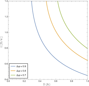
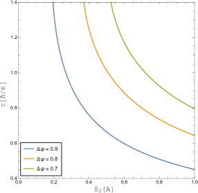
Figure 1: Left panel: Evolution time $\tau$ (in units of $\hbar/\epsilon$) as a function of entanglement entropy $S(A)$ for different distances $\Delta\psi$. Right panel: Evolution time $\tau$ (in units of $\hbar/\epsilon$) as a function of quadratic entanglement entropy $S_{2}(A)$ for different distances $\Delta\psi$.

Using Eqs. 5 and 9, we plot in the left panel of Fig. 1 the evolution time $\tau$ as a function of $S(A)$ for different values of $\Delta\psi$. Similarly, using Eqs. 6 and 9, we plot in the right panel of Fig. 1 the evolution time $\tau$ as a function of $S_{2}(A)$ for different values of $\Delta\psi$. From Fig. 1, we see that the more entanglement the system has, the further and faster its state vector can move.

II.2 A single qubit clock

To gain some initial intuition, we first consider the simplest case of a qubit clock that is entangled with the system as follows boette :

$$\ket{\Psi\rangle}=\frac{1}{\sqrt{2}}\left(\ket{0}_{T}\ket{\psi_{0}}_{S}+\ket{1}_{T}\ket{\psi_{1}}_{S}\right).$$ (10)

The system evolves from the initial state $\ket{\psi_{0}}_{S}$ to the final state $\ket{\psi_{1}}_{S}$ while the qubit clock ticks from $\ket{0}_{T}$ to $\ket{1}_{T}$. The double ket notation of $\ket{\Psi}\rangle$ is just to remind us that it is the static “global state” and not the evolving state of the system. The reduced density matrix of the system is

$$\rho_{S}=\mathrm{Tr}_{T}(\ket{\Psi\rangle}\bra{\langle\Psi})=\frac{1}{2}(\ket{\psi_{0}}\bra{\psi_{0}}+\ket{\psi_{1}}\bra{\psi_{1}}),$$ (11)

whose the nonzero eigenvalues are

$$p_{\pm}=\frac{1\pm|\braket{\psi_{1}}{\psi_{0}}|}{2},$$ (12)

which can also be obtained from Eq. 22 below by substituting $N=2$. The time-system entanglement entropy is then

$$E(T,S)=-\mathrm{Tr}(\rho_{S}\log_{2}\rho_{S})=-\sum_{k=\pm}p_{k}\log_{2}p_{k}.$$ (13)

The quadratic time-system entanglement entropy is

$$E_{2}(T,S)=2(1-\mathrm{Tr}(\rho_{S}^{2}))=4p_{+}p_{-}.$$ (14)

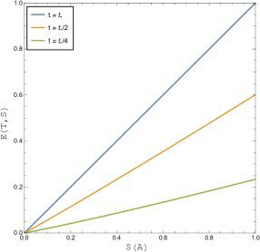
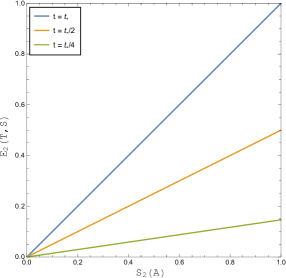
Figure 2: A single qubit clock. Left panel: Time-System entanglement entropy $E(T,S)$ as a function of $S(A)$ for different times. Right panel: Quadratic time-system entanglement entropy $E_{2}(T,S)$ as a function of $S_{2}(A)$ for different times.

From Eq. 12, we see that the more the system evolves, the more it becomes entangled with time. From Eq. 8, we see that, for a given state with a fixed $|\alpha|^{2}$, the minimum time at which the fidelity is minimum is

$$t_{*}=\frac{\pi\hbar}{2\epsilon}.$$ (15)

This time corresponds to the maximum time-system entanglement. Using Eqs. 13 and 5, we can plot $E(T,S)$ as a function of $S(A)$. Similarly, using Eqs. 14 and 6, we can plot $E_{2}(T,S)$ as a function of $S_{2}(A)$. These two plots are shown in Fig. 2.

From Fig. 2, we have two remarks:

• For a given time interval, we see that if the system has more entanglement within itself, then it becomes more entangled with time as it evolves. Combining this result with Fig. 1, we can now see the whole picture: The more internal entanglement the system has, the faster it can evolve. Therefore, during a fixed time interval, the state vector can travel through a larger distance in Hilbert space and thus becomes more entangled with time.

• The patterns of $E(T,S)$ and $E_{2}(T,S)$ are quite similar, though the scale of the former is slightly greater than that of the latter.

II.3 Continuous quantum time

We now generalize our results to the continuous limit where there are infinitely many steps of evolution between the initial and final states. A useful procedure is to consider the global state boette

$$\ket{\Psi\rangle}=\frac{1}{\sqrt{N}}\sum_{t^{\prime}=0}^{N-1}\ket{t^{\prime}}_{T}\otimes\ket{\psi(t^{\prime})}_{S},$$ (16)

and then take the limit $N\rightarrow\infty$ in the end. The normalization factor here indicates that each moment of time is equally likely to be occupied by the system’s evolution. By taking the limit $N\rightarrow\infty$, it is also true to say that the system’s evolution generates an infinite-dimensional Hilbert space of quantum time. The state vector at time $t$ is

$$\ket{\psi(t)}=\alpha\ket{00}+\beta e^{-i\theta_{t}}\ket{11},$$ (17)

where $\theta_{t}\equiv 2\epsilon t/\hbar$ for brevity. Note that $\ket{\psi(t^{\prime})}=\alpha\ket{00}+\beta e^{-i\theta_{t}\frac{t^{\prime}}{N-1}}\ket{11}$, so the state vector moves from the initial state $\ket{\psi(0)}$ to the target state $\ket{\psi(t)}$ in $N-1$ steps.

The reduced density operator of the system is

$$\rho_{S}=\mathrm{Tr}_{T}(\ket{\Psi}\rangle\langle\bra{\Psi})=|\alpha|^{2}\ket{00}\bra{00}+\gamma(t)\ket{00}\bra{11}+\gamma(t)^{*}\ket{11}\bra{00}+|\beta|^{2}\ket{11}\bra{11},$$ (18)

where

$$\gamma(t)\equiv\alpha\beta^{*}\braket{T_{1}}{T_{0}},$$ (19)

$$\ket{T_{0}}\equiv\frac{1}{\sqrt{N}}\sum_{t^{\prime}=0}^{N-1}\ket{t^{\prime}},$$ (20)

$$\ket{T_{1}}\equiv\frac{1}{\sqrt{N}}\sum_{t^{\prime}=0}^{N-1}e^{-i\theta_{t}\frac{t^{\prime}}{N-1}}\ket{t^{\prime}}.$$ (21)

The nonzero eigenvalues of the reduced density matrix $\rho_{S}$ are

$$p_{\pm}=\frac{1\pm\sqrt{1-4(|\alpha|^{2}(1-|\alpha|^{2})-|\gamma(t)|^{2})}}{2},$$ (22)

where

$$|\gamma(t)|^{2}=\frac{|\alpha|^{2}(1-|\alpha|^{2})}{N^{2}}\Bigg{|}\sum_{t^{\prime}=0}^{N-1}e^{i\theta_{t}\frac{t^{\prime}}{(N-1)}}\Bigg{|}^{2}=\frac{|\alpha|^{2}(1-|\alpha|^{2})}{N^{2}}\frac{\cos\left(\frac{N\theta_{t}}{N-1}\right)-1}{\cos\left(\frac{\theta_{t}}{N-1}\right)-1}.$$ (23)

In the continuous limit, this reduces to

$$\lim_{N\rightarrow\infty}|\gamma(t)|^{2}=2|\alpha|^{2}(1-|\alpha|^{2})\frac{1-\cos\theta_{t}}{\theta_{t}^{2}}.$$ (24)

The entanglement measures can then be calculated as usual by taking the continuous limit $N\rightarrow\infty$:

$$E(T,S)=\lim_{N\rightarrow\infty}\left(-\sum_{k=\pm}p_{k}\log_{2}p_{k}\right),$$ (25)

$$E_{2}(T,S)=\lim_{N\rightarrow\infty}\left(4p_{+}p_{-}\right).$$ (26)

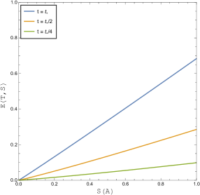
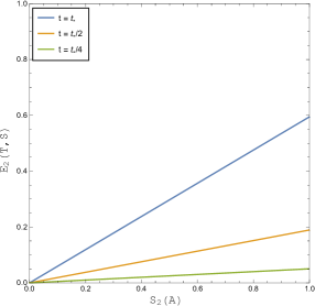
Figure 3: Continuous quantum time. Left panel: Time-System entanglement entropy $E(T,S)$ as a function of $S(A)$ for different times. Right panel: Time-System quadratic entanglement entropy $E_{2}(T,S)$ as a function of $S_{2}(A)$ for different times.

Using Eqs. 25 and 5, we can plot $E(T,S)$ as a function of $S(A)$. Similarly, using Eqs. 26 and 6, we can plot $E_{2}(T,S)$ as a function of $S_{2}(A)$. These plots are shown in Fig. 3. From Fig. 3, we have two remarks:

• The two remarks written in the end of Sec. II.2 continue to hold. Namely, increasing internal entanglement speeds up the evolution and makes the system more entangled with time. The scale of $E_{2}(T,S)$ is slightly less than that of $E(T,S)$.

• In the continuous limit, we see that the time-system entanglement entropies are smaller than that of the single qubit clock case. In other words, if the state vector has to travel through more intermediate steps between the initial and final states, it becomes less entangled with time boette .

III Evolution with quantum time: Two interacting qubits

We now consider the case where entanglement between two qubits is generated by interaction between them. We focus on computing the time-system entanglement entropy in the continuous limit. The Hamiltonian is given by

$$H_{total}=H_{A}\otimes I_{B}+I_{A}\otimes H_{B}+H_{int},$$ (27)

where the local Hamiltonians $H_{A}$ and $H_{B}$ were defined in Eqs. 2 and 3, and the interacting Hamiltonian is

$$H_{int}=-\lambda(\ket{1}\bra{0}\otimes\ket{1}\bra{0}+\ket{0}\bra{1}\otimes\ket{0}\bra{1}),$$ (28)

where $\lambda$ is a real coupling constant that has dimension of energy. This interacting Hamiltonian is capable of generating entanglement between two qubits. One can also add a constant term to the total Hamiltonian but that will only introduce an irrelevant overall phase factor. The initial state is a factorized state:

$$\ket{\psi(0)}=\ket{00}.$$ (29)

The state vector at time $t$ is given by the formal solution to the Schrodinger equation:

$$\ket{\psi(t)} =e^{-i\int H_{tot}dt/\hbar}\ket{00}$$ (30)

$$=\cos\frac{\lambda t}{\hbar}\ket{00}+i\sin\frac{\lambda t}{\hbar}\ket{11}$$ (31)

$$\equiv\cos\phi_{t}\ket{00}+i\sin\phi_{t}\ket{11},$$ (32)

where we used the fact that $H_{A}\ket{0}_{A}=H_{B}\ket{0}_{B}=0$ and $H_{int}\ket{00}=\ket{11}$ and $H_{int}\ket{11}=\ket{00}$. We also defined $\phi_{t}\equiv\lambda t/\hbar$ in the last line for brevity.

The global state is

$$\ket{\Psi}\rangle=\frac{1}{\sqrt{N}}\sum_{t^{\prime}=0}^{N-1}\ket{t^{\prime}}\otimes\ket{\psi(t^{\prime})}.$$ (33)

Here $\ket{\psi(t^{\prime})}=\cos\left(\phi_{t}\frac{t^{\prime}}{N-1}\right)\ket{00}+i\sin\left(\phi_{t}\frac{t^{\prime}}{N-1}\right)\ket{11}$, so the state vector moves from the initial state $\ket{\psi(0)}$ to the target state $\ket{\psi(t)}$ in $N-1$ steps. The reduced density operator of the system is

$$\rho_{S}=\mathrm{Tr}_{T}(\ket{\Psi}\rangle\langle\bra{\Psi})=a(t)\ket{00}\bra{00}+c(t)\ket{00}\bra{11}+c^{*}(t)\ket{11}\bra{00}+b(t)\ket{11}\bra{11},$$ (34)

where

$$a(t)\equiv\frac{1}{N}\sum_{t^{\prime}=0}^{N-1}\cos^{2}\left(\phi_{t}\frac{t^{\prime}}{N-1}\right),$$ (35)

$$b(t)\equiv\frac{1}{N}\sum_{t^{\prime}=0}^{N-1}\sin^{2}\left(\phi_{t}\frac{t^{\prime}}{N-1}\right),$$ (36)

$$c(t)\equiv-\frac{i}{2N}\sum_{t^{\prime}=0}^{N-1}\sin\left(2\phi_{t}\frac{t^{\prime}}{N-1}\right).$$ (37)

The nonzero eigenvalues of the system density operator $\rho_{S}$ are

$$p_{\pm}=\pm\frac{1}{4N}\csc^{2}\left(\frac{\phi_{t}}{N-1}\right)\left[\pm N\left(1-\cos\left(\frac{2\phi_{t}}{N-1}\right)\right)+2\sqrt{\sin^{2}\left(\frac{\phi_{t}}{N-1}\right)\sin^{2}\left(\frac{N\phi_{t}}{N-1}\right)}\right].$$ (38)

In the continuous limit, this reduces to

$$\lim_{N\rightarrow\infty}p_{\pm}=\frac{1}{2}\left(1\pm\frac{\sin\phi_{t}}{\phi_{t}}\right).$$ (39)

Time-system entanglement entropy is then

$$E(T,S)=\lim_{N\rightarrow\infty}\left(-\sum_{k=\pm}p_{k}\log_{2}p_{k}\right).$$ (40)

The fidelity between the initial and final states is

$$\Delta\psi=|\braket{\psi(t)}{\psi(0)}|=\cos\phi_{t},$$ (41)

and thus

$$\phi_{t}=\arccos\Delta\psi.$$ (42)

The minimum time required for the initial state to evolve to the orthogornal final state is

$$t_{*}^{I}=\frac{\pi\hbar}{2\lambda}.$$ (43)

Comparing Eq. 43 with Eq. 15, we see that the speed of evolution of two interacting qubits is greater than that of two non-interacting qubits if the interaction is sufficiently strong compared to the energy scale of the individual subsystems: $\lambda>\epsilon$.

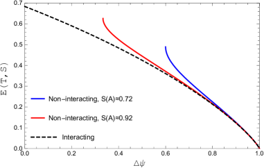
Figure 4: Time-system entanglement entropy E(T,S) as a function of fidelity $\Delta\psi$. Blue line: two non-interacting qubits with $S(A)\approx 0.72$ corresponding to $|\alpha|^{2}=1/5$ or $|\alpha|^{2}=4/5$. Red line: two non-interacting qubits with $S(A)\approx 0.92$ corresponding to $|\alpha|^{2}=1/3$ or $|\alpha|^{2}=2/3$. Dashed black line: two interacting qubits with time-dependent internal entanglement. The line of two maximally entangled but non-interacting qubits ($S(A)=1$) coincides with the interacting line, though it should be noted that the speed of evolution in the two cases is different (see Eqs. 15 and 43).

Using Eqs. 40 and 42, we can plot $E(T,S)$ as a function of fidelity in Fig. 4. The interacting case is represented by dashed black line. From Fig. 4, we see that $E(T,S)$ increases when fidelity decreases. That is because the more the system evolves, the more it becomes entangled with time. When the state vector reaches its maximum distance at $\Delta\psi=0$ (i.e. it evoles to an orthorgonal state), the corresponding entropy it can acquire is $E_{\perp}(T,S)\approx 0.68$.

Also in Fig. 4, we plotted two solid colorful lines to represent the case of two non-interacting qubits by using Eqs. 8 and 24. These lines are cut at the maximum distances that the corresponding state vectors can travel. Among the non-interacting cases, we see that increasing internal entanglement speeds up the evolution, since the state vector can travel further in a fixed time interval, and makes the system more entangled with time. If two non-interacting qubits are maximally entangled, its line coincides with the interacting line, though it should be noted that the speed of evolution in the two cases, in general, is different (see Eqs. 15 and 43).

IV Conclusions

In this paper, we studied the entanglement between quantum time and a quantum system containing two entangled qubits. We considered the case of two initially entangled qubits evolving under local dynamics, as well as the case of two interacting qubits such that their internal entanglement is generated over time. In the first case, we obtained the main result that increasing internal entanglement speeds up the evolution and makes the system more entangled with time. In the second case, we showed the dependence of time-system entanglement entropy on the distance of evolution which is characterized by fidelity. We compared the two cases with each other and found that two interacting qubits can evolve faster than two non-interacting qubits if the interaction is sufficiently strong, and thus they become entangled with time more efficiently.

Our results could be useful to gain new insights of quantum time into black hole evaporation or cosmological perturbations in an expanding Universe, since we also have an evolving entangled bipartite system in those cases. For black hole, the total Hilbert space is decomposed on a spatial slice as $\mathcal{H}_{tot}=\mathcal{H}_{in}\otimes\mathcal{H}_{out}$, where $\mathcal{H}_{in}$ contains infalling degrees of freedom and $\mathcal{H}_{out}$ contains outgoing Hawking quanta. For cosmological perturbations, the Hilbert space can be decomposed in momentum space as $\mathcal{H}_{tot}=\mathcal{H}_{k>aH}\otimes\mathcal{H}_{k<aH}$, where $\mathcal{H}_{k>aH}$ contains subhorizon modes and $\mathcal{H}_{k<aH}$ contains superhorizon modes. In both cases, the system can be an evolving pure state that contains two entangled subsystems. It is therefore interesting to see how our idea can be applied to those cases and if quantum time can offer new insights into the information paradox in each case Hawking ; loc2 . We plan to investigate further along these lines.

References

- (1) Asher Peres, Petra F. Scudo, and Daniel R. Terno, Quantum Entropy and Special Relativity, Phys. Rev. Lett. 88, 230402 (2002).
- (2) Robert M. Gingrich and Christoph Adami, Quantum Entanglement of Moving Bodies, Phys. Rev. Lett. 89, 270402 (2002).
- (3) Don N. Page and William K. Wootters, Evolution without evolution: Dynamics described by stationary observables, Phys. Rev. D 27, 2885 (1983).
- (4) Ngo Phuc Duc Loc, Time-System Entanglement and Special Relativity, arXiv:2212.13348
- (5) A. Boette, R. Rossignoli, N. Gigena, and M. Cerezo, System-time entanglement in a discrete-time model, Phys. Rev. A 93, 062127 (2016).
- (6) L. Mandelstam and I. G. Tamm, J. Phys. (Moscow) 9, 249 (1945).
- (7) N. Margolus and L. B. Levitin, Physica D 120, 188 (1998).
- (8) Ahmed Almheiri, Thomas Hartman, Juan Maldacena, Edgar Shaghoulian, and Amirhossein Tajdini, The entropy of Hawking radiation, Rev. Mod. Phys. 93, 035002 (2021).
- (9) Ngo Phuc Duc Loc, Unitary paradox of cosmological perturbations, Int. J. Mod. Phys. D 32, 2350050 (2023).