GIO: Gradient Information Optimization for Training Dataset Selection

Abstract

It is often advantageous to train models on a subset of the available train examples, because the examples are of variable quality or because one would like to train with fewer examples, without sacrificing performance. We present Gradient Information Optimization (Gio), a scalable, task-agnostic approach to this data selection problem that requires only a small set of (unlabeled) examples representing a target distribution. Gio begins from a natural, information-theoretic objective that is intractable in practice. Our contribution is in showing that it can be made highly scalable through a simple relaxation of the objective and a highly efficient implementation. In experiments with machine translation, spelling correction, and image recognition, we show that Gio delivers outstanding results with very small train sets. These findings are robust to different representation models and hyperparameters for Gio itself. Gio is task- and domain-agnostic and can be applied out-of-the-box to new datasets and domains.

1 Introduction

In situations in which one has a very large train set available, it is often advantageous to train systems on a subset of the data. In the simplest case, the train set may be so large as to run up against resource constraints, and the question arises whether performance goals can be reached with less effort (e.g. Touvron et al., 2021). It can also be the case that the train examples are known to be of variable quality, say, because they were harvested from diverse websites (Luccioni and Viviano, 2021), annotated by crowdworkers (Karpinska et al., 2021), or created by a synthetic data generation process (Edunov et al., 2018). In this case, the goal is to identify a reliable subset of examples.

This is the data selection problem that we address in the current paper. The end goal is to select a subset of the available train examples that leads to models that are at least as performant as (and perhaps even better than) those trained on all the examples. To achieve this goal, we propose Gradient Information Optimization (Gio), a highly scalable, task-agnostic approach to data selection that is based in information theory. Our method assumes access to a (potentially small) set of examples $X$ that represent the desired data distribution and a (presumably very large) set of potential train examples $G$. Our method derives a set $V\subseteq G$ that has as much information content as possible about the target distribution $X$. The method begins from the natural intuition that we want $V$ to minimize the average KL divergence from $X$, and the novelty of the approach lies in making this computationally tractable by relying on properties of the derivative of the KL divergence and implementing the method extremely efficiently. Crucially, our method works in any continuous representation space, is task- and domain-agnostic, and requires no labels on examples.

We motivate Gio with a diverse set of experiments. We first explore machine translation using the WMT14 dataset and Transformer-based models. In this case, $G$ is the WMT14 dataset and $X$ is the dev set. These experiments show that, using Gio, we can can surpass the performance of a model trained on the full WMT14 corpus with only a fraction of the example in $G$, which represents very large efficiency gains. We then turn to spelling correction. In this case, the set $G$ is generated by a noisy synthetic process and the target distribution $X$ is a set of actual spelling errors. Here, we are using Gio to home in on realistic train examples. Our results show that we can do this extremely effectively. Finally, we apply Gio to an image recognition task (FashionMNIST) and show again that our method can reduce the size of the train sets chosen without large drops in performance, this time operating with representations of images. In this case, we trust the train set $G$ to represent the space accurately, and our goal is simply to select a useful subset of $G$. Thus, in this case $X=G$. Finally, we discuss expanding Gio, report on a wide range of robustness experiments and empirical analyses of how and why the method works in practice, and publish a pip-installable package.

2 Related Work

Active learning.

Active learning methods (e.g. Sener and Savarese, 2018, Gal et al., 2017, Kirsch et al., 2019) can be cast as data selection methods in our sense. In active learning, one iteratively chooses new unlabeled training examples to label, with the goal of efficiently creating a powerful train set. By contrast, Gio makes no use of labels and is oriented towards the goal of identifying a subset of existing cases to use for training. Additionally, active learning is most suited to classification problems, whereas Gio works with any arbitrary task.

Heuristic.

Gio is closer to recent methods in which one uses a large language model to generate a large number of candidate texts and then extracts a subset of them based on a specific criteria. For example, Brown et al. (2020) develop a heuristic method to filter CommonCrawl based on a trained classifier’s probability that datapoints are high quality. Similarly, Wenzek et al. (2020) develop a pipeline to clean CommonCrawl based principally on the perplexity of an LM trained on high quality text, and Xie et al. (2023) develop a sampling technique based on approximate n-gram counts.

Like Gio, these heuristic methods aim to select a subset of data that is higher quality and more relevant. However, they are either highly tailored to their particular tasks or they require very large numbers of examples (to develop classifiers or construct target probabilities). By contrast, Gio is task- and domain-agnostic, it can be applied plug-and-play to a new task and dataset, and it requires comparatively few gold examples $X$ to serve as the target distribution.

Similarity Search.

Methods using vector or n-gram similarity search can also be used for data selection at scale (e.g. Johnson et al., 2017, Bernhardsson, 2017, Santhanam et al., 2022). The technique would index $G$ and $X$ and retrieve the top-k datapoints from $G$ for each point in $X$. Like our method, similarity search works in a continuous space. However, similarity search can be prone to selecting suboptimal points; we review such a case in detail in Section 3.4. Additionally, similarity search does not have a natural stopping criterion and requires data size to be chosen arbitrarily. Is 10% data enough? 20%? We don’t know a priori. And if the data in $G$ is far away from $X$, similarity search will still choose it up to the desired data size. Recently, Yao et al. (2022) use a BM25 retrieval method for data selection, with strong results. However, BM25 operates on a bag-of-words model, which can make it challenging when the target set is small, and like any similarity search, requires data size to be chosen arbitrarily beforehand. Further, this method only applies to text tasks, whereas Gio applies to any task with continuous representation.

Data Pruning.

Data pruning has shown promise for the data selection problem (e.g. Paul et al., 2021). Different works in data pruning use varied approaches, but generally iteratively identify and add optimal samples from training data. However, most works in data pruning (e.g. Paul et al., 2021, Yang et al., 2023, Saseendran et al., 2019) apply only to classification. However, recently Sorscher et al. (2022) develop a self-pruning method with strong results that can be applied to any task with continuous representation, like Gio, using clustering-based selection. Unlike Gio and similarity search however, self-pruning does not consider any desired target distribution $X$.

Submodular Optimization.

Submodular optimization methods have also been proposed for data selection (Kaushal et al., 2022), where an optimizer optimizes a submodular function between a general set $G$ and a target set $X$. Like Gio, submodular optimization takes into account a desired target distribution $X$, has a natural stopping criterion that does not require data size to be chosen arbitrarily. Unlike Gio however, submodular optimization is restricted only to submodular functions, which have certain assumptions that may not hold true. For example, submodular functions assume adding each extra datapoint diminishes the return of that datapoint, which is not necessarily the case when constructing a dataset. For example, if we have already have selected data but have unexplored region where $X$ has a mode, adding data in that region does not exhibit a diminishing return. Gio, on the other hand, makes no assumptions on the functions it can use.

Overall, previous work in data selection is typically tailored to a specific domain like NLP (e.g. Wenzek et al., 2020) or image recognition (e.g. Gal et al., 2017), and makes assumptions about the data available, for example, that the target set $X$ is large enough to construct an LM (e.g. Wenzek et al., 2020), or that it has labels (e.g. Sener and Savarese, 2018). In addition, many of these methods use discrete approximations and heuristics (e.g. Xie et al., 2023, Yang et al., 2020). In this work, we provide a general, theoretically-motivated data selection method that works with large or small $X$ and can be applied out-of-the-box to any domain (image, text, etc) without needing labels.

Algorithm 1 Gradient Information Optimization

Quantize $X,D,G$ using K-means and pick the cluster centroids $X_{c},D_{c},G_{c}$ as the new points

while Not Stopping Criterion do

     Gradient-Descend to find $\mathbf{v}_{opt}$:

          $\mathbf{v}_{1}\leftarrow$ previous $\mathbf{v}_{\textit{opt}}$, $\bar{\mathbf{x}}$ or random $\triangleright$ We explore different techniques in our experiments

          Perform $\mathbf{v}_{k+1}\leftarrow\mathbf{v}_{k}-\gamma\cdot\frac{\partial}{\partial\mathbf{v}_{k}}\hat{D}_{\textit{KL}}(P_{X_{c}}\parallel P_{D_{c}\cup\{\mathbf{v}_{k}\}})$ until converged to $\mathbf{v}_{\textit{opt}}$

     Update $D_{c}$ :

          $\mathbf{v}_{b}\leftarrow\operatorname*{argmin}_{\mathbf{v}_{i}\in G_{c}}||\mathbf{v}_{i}-\mathbf{v}_{\textit{opt}}||$ $\triangleright$ The closest point in $G_{c}$ to $\mathbf{v}_{\textit{opt}}$

          $D_{c}\leftarrow D_{c}+\{\mathbf{v}_{b}\}$

          Remove $\mathbf{v}_{b}$ from $G_{c}$

end while

Explode: Select points from full $D$ and $G$ which belong to the chosen centroids’ ($D_{c}\cup V_{c}$) clusters

3 Gradient Information Optimization: Method

We formulate data selection as maximizing information content and outline the natural algorithm for this objective, which is infeasible. We then introduce optimizations which enable the algorithm to work at scale, and conduct tests to show the algorithm is consistent and robust to different scenarios.

3.1 Abstract Formulation of the Data Selection Problem

We assume that all examples are represented in continuous space. We have a set of train examples $G$ and a target ideal state $X$. We allow also that there may be existing train examples $D$ that we definitely want to include in our train set, though $D$ can be empty. Our goal is to identify a subset $V$ of $G$ such that the set $D\cup V$ contains the most information about $X$.

In this setting, it is natural to take an information-theoretic approach. Let $p_{X}(\mathbf{x})$ be the distribution of target $X$, and let $p_{D\cup V}(\mathbf{x})$ be the distribution of selected data $D\cup V$. The information content of $D\cup V$ about $X$ is the negative KL divergence from $p_{X}(\mathbf{x})$ to $p_{D\cup V}(\mathbf{x})$ (Kullback and Liebler, 1951). In this context, the general objective of data selection is as follows:

Choose data $$V\subseteq G \int_{\Omega}p_{X}(\mathbf{x})\log\frac{p_{X}(\mathbf{x})}{p_{D\cup V}(\mathbf{x})}d\mathbf{x}$$ such that is minimized (1)

The implication is that a data selection method which gives the minimum KL divergence will also give the best performance (assuming we are correct that $X$ represents the task to be solved).

3.2 Naive Approach

A natural approach is to hill-climb on the KL divergence objective (1). Given existing data $D$ and points $\mathbf{v}_{1},\ldots,\mathbf{v}_{k}$ of $G$, we recompute the distribution $p_{D\cup\{\mathbf{v}_{i}\}}(\mathbf{x})$ for each $\mathbf{v}_{i}$, pick the one that gives the minimum KL divergence, and add it to our selected set $D$:

$$D\leftarrow D+\operatorname*{argmin}_{\mathbf{v}_{i}\in G}\displaystyle\int_{\Omega}p_{X}(\mathbf{x})\log\frac{p_{X}(\mathbf{x})}{p_{D\cup\{\mathbf{v}_{i}\}}(\mathbf{x})}d\mathbf{x}$$ (2)

Unfortunately, this algorithm is intractable in practice. We need to construct a new distribution $p_{D\cup\{\mathbf{v}_{i}\}}(\mathbf{x})$ and compute KL divergence for every $\mathbf{v}_{i}\in G$, at each step. Therefore, the complexity at each iteration is $\mathcal{O}(|G|\cdot C)$, where $C$ is the cost of computation for the KL divergence. For a dataset of only 1M and 0.1s per iteration, it would take 70 days to complete the algorithm. The method is also prone to adding the same point multiple times.

3.3 Gradient Information Optimization

Gio addresses the shortcomings of (2) with a combination of mathematical and implementational optimizations. The method is described in Algorithm 1.

First, instead of calculating divergence for each point, we use the derivative of the KL divergence to find the optimal point. We rewrite $p_{D\cup\{\mathbf{v}_{i}\}}(\mathbf{x})=g(\mathbf{x},\mathbf{v}_{i})$, a function of only $\mathbf{x}$ and $\mathbf{v}_{i}$ since $D$ is not changing, and thus the optimization term in each iteration becomes:

$$\operatorname*{argmin}_{\mathbf{v}_{i}\in G}\int_{\Omega}p_{X}(\mathbf{x})\log\frac{p_{X}(\mathbf{x})}{g(\mathbf{x},\mathbf{v}_{i})}d\mathbf{x}$$ (3)

We can relax the constraint that $\mathbf{v}_{i}\in G$ to the space of all possible $\mathbf{v}$ and solve this integral minimization for the optimal $\mathbf{v}_{\textit{opt}}$. Since $p_{X}$ is unchanging and the integral implicitly removes $\mathbf{x}$ as a variable, the integral defines a functional $F\left[g(\mathbf{v})\right]$ . Therefore, we partially differentiate with respect to $\mathbf{v}$ and do gradient descent with the partials $\nabla_{\mathbf{v}_{k}}F[g]$ to solve for $\mathbf{v}_{\textit{opt}}$. All together, this becomes:

$$\mathbf{v}_{k+1}\leftarrow\mathbf{v}_{k}-\gamma\cdot\frac{\partial}{\partial\mathbf{v}_{k}}\left(\int_{\Omega}p(\mathbf{x})\log\frac{p(\mathbf{x})}{g(\mathbf{x},\mathbf{v}_{k})}d\mathbf{x}\right)$$ (4)

Once we have $\mathbf{v}_{\textit{opt}},$ we find the nearest $\mathbf{v}_{i}\in G$ and add that to $D$, as the closest $\mathbf{v}_{i}\in G$ is the solution to the original (3). For that to be true, we assume $G$ is locally dense for the extrema of the integral in (4); see Appendix A.2 for details.

The complexity at each iteration, for $S$ gradient descent steps, is $\mathcal{O}(S\cdot C)$ which does not increase with $G$. Therefore, when $|G|>S$, as is common in practice, the derivative trick is faster than the naive algorithm. We time both algorithms in Section 3.4 and show the derivative trick is 80% faster.

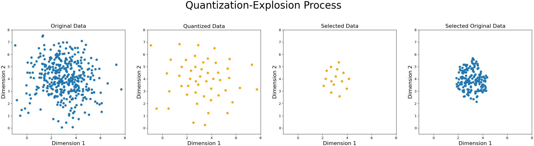
Figure 1: Visualization of the Quantization-Explosion Process. From left to right: original data (400 points), representative K-means centroids (50 points) of the original data (Quantization), selected centroids after data selection, original data represented by the selected centroids (Explosion)

Second, even at its most efficient, an algorithm that adds point-by-point becomes intractable. Therefore, we use a quantization-explosion process. First, we cluster the data with K-means (Arthur and Vassilvitskii, 2007) and pick the centroids $\boldsymbol{\mu}_{i}$ as our new data points. Second, we perform the algorithm using the cluster centroids $\boldsymbol{\mu}_{i}$ instead of the original data. Finally, after having our chosen cluster centroids, we explode back out into the original data based on cluster membership. Figure 1 provides an overview of this process.

Third, to compute the KL Divergence in high-dimensional spaces, we use the k-Nearest Neighbors approximation for continuous KL divergence proposed by Wang et al. (2009), and modify it to be an average across all points to bypass 0 gradient problems (details and proof of modification are in the Appendix A.1). Let $|D|=m$, $|X|=n$ and $d$ be the dimensionality:

$$\hat{D}_{\textit{KL}}(P_{X}\parallel P_{D})=\frac{1}{m}\sum_{k=1}^{m}\frac{1}{n}\left[\sum_{i=1}^{n}d\cdot\log\nu_{k}(i)-d\cdot\log\rho_{l}(i)\right]+\frac{1}{m}\sum_{k=1}^{m}\log\frac{l\cdot m}{k(n-1)}$$ (5)

Where $\nu_{k}(i)$ is the distance from point $X_{i}$ to the $k$th nearest point in $D$ and $\rho_{l}(i)$ is the distance from point $X_{i}$ to the $l$th nearest $X_{j\neq i}$. We use automatic differentiation to compute the derivative.

We can stop when the KL divergence increases, reset $G$ and allow the algorithm to pick again, among a variety of criteria. We explore several in our experiments and list additional criteria in Appendix B.2. Unlike data selection methods that make data size a hyperparameter (e.g. Yao et al., 2022), Gio provides a natural stopping criterion (KL divergence). Finally, initializing $D$ from a uniform start rather than empty leads to same optimal points but a smoother convergence; see Appendix A.3.

Limitations.

We derived Gio from the natural information-theoretic objective, however, we can use any arbitrary statistical distance in the Gio framework. For example, in situations where $G$ is close to $X$ with the exception of a large gap somewhere, the statistical distance $\max|p_{X}(\mathbf{x})-p_{D}(\mathbf{x})|$ may be better suited. We also use gradient descent to iteratively find $\mathbf{v}_{\textit{opt}}$, but we know the space is non-convex. Therefore, replacing gradient descent with a method like particle swarm optimization (Kennedy and Eberhart, 1995) may lead to better selected data. Finally, in practice it is important to ensure that $X$ reasonably represents the space a model might be used on. A narrow $X$ could make a model trained on Gio-selected data perform poorly when confronted with inputs that lie outside $X$. Methods like starting from a subset of training data, which we explore, or adding uniform points to $X$ to encourage generalization, should be explored. We leave these improvements to future work.

3.4 Analytic Checks

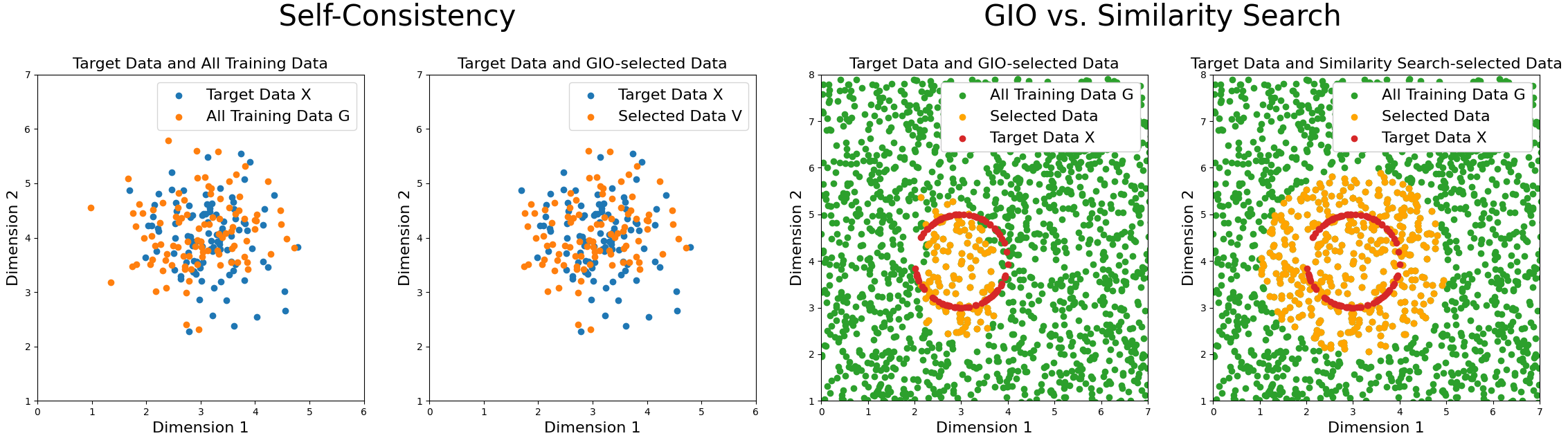
Figure 2: The leftmost graph shows $X$ and $G$, which come from the same distribution. The second graph shows that Gio recovers nearly all of $G$ (self consistency). The right two graphs compare Gio with similarity search. Points within the circle formed by $X$ are more ideal than points outside. By considering the distribution, Gio selects nearly all points inside before terminating (third graph). By comparison, in order to pick points within the circle, similarity search also picks a range of points outside the circle, which is suboptimal (fourth graph).

Gio is self-consistent.

We define self-consistency as follows: if both $G$ and $X$ come from the same distribution, i.e., $p_{G}(\mathbf{x})=p_{X}(\mathbf{x})$, a good data selection method should choose all of $G$. We show Gio is self-consistent with the following setup: let $X$ be 100 points from a normal distribution centered at $(3,4)$ and let $G$ be another 100 points from the same distribution (Figure 2, 1^st graph). We run Gio on this setup; Gio selects 96% of $G$ before termination, showing Gio is self-consistent (Figure 2, 2^nd graph).

Gio is negative-consistent.

We define negative consistency as follows: if $G$ is very far from $X$, i.e. $d(p_{X}(\mathbf{x}),p_{G}(\mathbf{x}))\gg 0$, a good data selection method should not choose any of $G$. Most data selection methods that rely on choosing a desired data size as a stopping criteria (e.g. Yao et al., 2022, Xie et al., 2023, similarity search) are not negative consistent; they will select data regardless of how close or far the data may be from $X$. We show Gio is negative-consistent with the following setup: let $X$ be the same as above, but this time let $G$ be 100 points centered far away at $(300,400)$. We run Gio on this setup; Gio terminates without adding any points from $G$, showing it is negative-consistent.

Quantization in Gio is consistent with the original space.

Quantizing the space with K-means should not change the distribution of data. We show the quantized space is consistent with the original space with the following setup: let $X$ be 400 points from a 2D normal distribution centered at $(3,4)$. We quantize $X$ using K-means with K=50, and compute the KL divergence $\hat{D}_{\textit{KL}}(X\parallel X_{\textit{quant}})$, which should be close to $0$ if the distributions are close. The KL divergence is $0.44$, showing the quantization in Gio is consistent with the original space.

The derivative trick is 80% faster.

We benchmark the wall-clock time between the naive hill-climb method and Gio with the derivative trick, with 100 points in $X$ and 2000 points in $G$ spread uniformly, and run the algorithm for 100 iterations. The regular hill-climb method takes 1369s, whereas the derivative trick takes 257s, representing an 80% speedup.

Gio selects based on a distribution; similarity search does not.

Let $X$ be a circle of 2D points encapsulating a region of space, and let $G$ be 2000 uniformly distributed points (Figure 2, 3^rd and 4^th graphs). The ideal points are the points within the region encapsulated by $X$ and should be chosen with preference over points outside. Figure 2 shows the points selected by semantic search (4^th graph); in order to get the data inside the circle, it also picks the data outside the circle. Figure 2 also shows the Gio-selected points (3^rd graph); by considering the distribution of all of $X$ rather than the simple Euclidean location of each $X$, Gio selects mostly points which are within the circle, as desired.

4 Experiments

We perform four sets of experiments to validate Gio. First, we replicate the setup of Vaswani et al. (2017) on WMT14 and show that using Gio can surpass the performance of the full model with a fraction of the data. Next, we demonstrate Gio is robust to different choices of embedding models and quantization. Third, we use a spelling correction task to show that Gio selects the highest quality data from a pool of mixed-quality synthetic data. Finally, we show Gio reduces the training set size of FashionMNIST image task without a big drop in performance. We show that Gio achieves the lowest KL divergence compared to alternatives, and that this correlates with model performance.

Table 1: Machine translation results. Training data sizes and BLEU scores of models trained on full data, Gio-selected data, comparative methods and random subsets for various initialization states. Bold is the best score in each initialization, italic is the best score overall. Gio outperforms a model trained with the full EN-FR with only 40% of the data and outperforms all comparative methods in 10/12 evaluations. It achieves 99% of the performance in EN-DE with only 60% of the data.

Init. %	System	EN-FR				EN-DE
		Train Size	Dev Test	WMT 14	$\mathbf{\hat{D}_{KL}}$	Train Size	Dev Test	WMT 14	$\mathbf{\hat{D}_{KL}}$
	Ours		34.2	41.2	156		22.1	24.3	148
	BM25		33.9	41.0	172		22.6	24.9	175
0	Pruning	05.6M	33.3	40.3	152	701K	22.0	24.2	177
	Submod.		33.8	40.8	170		22.0	24.5	164
	Random		33.1	40.0	194		21.9	24.0	183
	Ours		34.8	42.2	166		23.9	27.0	159
	BM25		34.6	42.0	179		22.9	26.3	178
25	Pruning	014M	34.1	41.4	174	1.7M	23.0	26.3	171
	Submod.		34.4	41.7	181		22.7	25.5	172
	Random		34.3	41.4	195		23.0	26.7	182
	Ours		34.7	42.3	172		24.2	27.9	164
	BM25		34.3	42.1	185		23.7	27.9	178
50	Pruning	021M	34.2	41.9	183	2.5M	23.6	27.1	179
	Submod.		34.4	41.7	185		21.9	24.5	176
	Random		34.1	41.7	195		24.0	27.3	181
100	Full	35M	-	41.8	188	4M	-	28.2	180

4.1 Machine Translation Experiments

Our first set of experiments seeks to show that Gio can pick data from a general corpus to meet or exceed the performance of a model trained on the full corpus.

Data and Methods

We use Transformer Big from Vaswani et al. (2017), trained for 300k iterations with the same hyperparameters. We use the same processed WMT14 training data. We report the BLEU score (Papineni et al., 2002) on the WMT14 test set.

We apply Gio to select a subset of data from the WMT14 train set using the inputs only (as our method makes no use of labels). $G$ is the training data we can select from. For target state $X$, we collect the dev sets for WMT08–WMT13, extract 3K pairs and report BLEU on this held out dev set, and use the remaining $\approx$12K pairs as $X$. For initial state $D$, we consider starting from an empty set, a 25% random subset of train data, and a 50% random subset of train data, and we report results for each setting. We use MPNet-Base-V2 model (Song et al., 2020) to embed the input sentences in a continuous vector space and use K=1500 for quantization. We compare this embedding model and quantization amount to other settings in our robustness experiments (Section 4.2). As our stopping criteria, we stop when the KL divergence increases. We also deduplicate the data pairs before training.

We compare Gio to a random subset of data of the same size. In addition, we compare against several competitive baselines with different approaches: Yao et al.’s (Yao et al., 2022) recent similarity search approach of BM25 retrieval, the recent data pruning self-pruning method introduced by Sorscher et al. (2022), and the submodular information optimization with mutual information as the function to optimize. To keep the setup equal, we also initialize each of the baselines from a 0%, 25% and 50% random subset and run those algorithms to have the same size as the Gio-selected data. For submodular optimization and self-pruning, we use the same clustering Gio is run with.

Results

We find that Gio outperforms the random baseline at every initialization. A data selection method should always outperform a randomly-selected subset of the same size. Table 1 shows the BLEU score on dev and WMT14 test sets and demonstrates Gio always outperforms random. BM25, submodular optimization and data pruning only outperform random sometimes.

Gio outperforms the EN-FR model trained on the full data using only 40% of the data. At initialization of 25% and 50%, a model trained on Gio-selected data outperforms the full Vaswani et al. (2017) model trained on all data by +0.4 and +0.6 BLEU, respectively. In addition, a model trained on the Gio-selected data at 0% initialization achieves 99% of the performance of the full model with only 16% of the data. It outperforms all comparative methods at all initializations. In EN-DE, it gets 99% of the performance with 60% of the data, and 88% of the performance with only 18% of the data.

Table 2: Training data sizes and BLEU scores of the base version (K=1500 and MPNet) and the variants of K and embedding model. BLEU scores of the variants vary by only 0.4% on average from the base, indicating Gio is robust to different quantization and embedding models

System		EN-FR				EN-DE
		Train Size	Dev Test	WMT 14	$\mathbf{\hat{D}_{KL}}$	Train Size	Dev Test	WMT 14	$\mathbf{\hat{D}_{KL}}$
Base (MPNet, K=1500)		5.6M	34.2	41.2	156	701K	22.1	24.3	148
MiniLM Variant		5.7M	34.0	41.1	-	737K	22.3	24.6	-
K=1000 Variant		5.6M	33.9	41.2	169	701K	22.1	24.3	150
K=3000 Variant		5.7M	34.2	41.3	138	718K	22.3	24.6	133
Average Variance from Base		1.9%	0.5%	0.2%	-	3.7%	0.6%	0.8%	-

Gio outperforms all comparative methods in 10/12 of the evaluations. Gio always matches or outperforms the comparative methods with initializations of 25% or 50%, by an average of +0.7 BLEU on WMT14 and +0.6 BLEU on Dev Test, and only falls short with 0% initialization in EN-DE.

Gio has the lowest KL divergence in 5/6 tests (Table 1), which correlates with model performance. The implication of the objective in (1) is that a method which results in lower KL divergence between train and target will perform the best. From Table 1, the average Spearman rank correlation coefficient between KL divergence and best performance is 0.83 and the median is 1, showing a high degree of correlation between a dataset that minimizes KL divergence and model performance, and thereby confirming the implication from the theory.

In summary, Gio leads to the lowest KL divergence between train and target set out of all the methods, which correlates with model performance and confirms the theory in (1). Notably, a model trained with Gio-selected data outperforms a model trained on the full data in EN-FR despite using only 40% of the total data and came to within 99% of the full model in EN-DE using only 60% of the data. Gio outperforms the random baseline at all initializations and outperforms all comparative methods in 10/12 evaluations. Overall, these experiments show Gio can achieve and surpass the performance of a model trained on full data and comparable baselines, by explicitly optimizing for KL Divergence.

4.2 Robustness

Gio above relies on two approximations to work: an embedding model, and K-means to quantize the space into representative samples of the full data. In this section, we show that Gio is robust to different embedding models and different values of K. The results are summarized in Table 2.

Gio works with different embedding models.

Gio should be robust to different text embedding models. We change the embedding model from MPNet-Base-V2 to MiniLM-L12-v1 (Wang et al., 2020), which has different architecture, training, and produces embeddings of a different size. We then rerun the 0% initialization experiments end-to-end with the new embeddings for both EN-DE and EN-FR. Table 2 shows that using MiniLM in Gio results in roughly similar selected data size (4.4% difference on average) and virtually identical performance (0.7% difference on average), demonstrating that Gio is robust to different embedding models.

Table 3: Spelling correction results. Training data size, % of high quality data and KL Divergence of the full data, Gio data, BM25 data, submodular optimization data, data pruning data and random subset. Bold is the best score overall. Gio selects 73% high quality data which outperforms all other methods.

System	Train Size	%High Quality	$\mathbf{\hat{D}_{KL}}$
Ours		73%	224
BM25		55%	264
Pruning	03.6M	54%	241
Submod.		59%	245
Random		50%	284
Full	14.7M	50%	280

Gio works with different choices of K.

Gio should also be robust to varying amounts of quantization. We decrease the value of K from 1500 to 1000 and increase to 3000 and rerun the 0% initialization experiments end-to-end for both new values of K, in EN-FR and EN-DE. For K=1000 due to the coarser grain, Gio selects more data, therefore we sample from the selected data the same amount as K=1500 in order to maintain parity. Table 2 shows that performance is virtually identical between the different values of K (0.4% difference on average), demonstrating Gio is robust to different values of K. In general, higher values of K have lower KL Divergence and slightly better performance, which is expected as the quantization is more fine grained.

4.3 Spelling Correction Experiments

In this section, we set up a problem with a pool of high and low quality synthetic candidate train examples and show Gio selects mostly high quality data. In addition, we set a new state of the art on the challenging BEA4660 spelling correction benchmark of Jayanthi et al. (2020); see Appendix C.

Data and Methods

We follow the setup of Jayanthi et al. (2020) and collect 15M samples from the 1 Billion Word benchmark corpus and deduplicate. To create high quality data, we use the best noising technique (prob) from Jayanthi et al. (2020) and noise half the data. For low quality data, we use the “word” method with high replacement rate (70%) and noise the other half, and mix the two sets.

We apply Gio to select a subset of data from the training set. $G$ is the training data we can select from. For target state $X$, Jayanthi et al. (2020) provide 40k real spelling mistakes and corrections from the BEA grammar correction corpus. For initial state $D$, we start from an empty set. For the embedding model, we use MPNet and K=1500 for quantization. As our stopping criteria, we experiment with a new scheme: first the algorithm runs until the KL divergence increases, then we reset $G$ and allow the algorithm to pick again from the training data, until the KL divergence decreases. As before, we compare Gio to a random subset of the same size and pruning, submodular and BM25 methods.

Results

Gio selects high quality data. A good data selection method should select mostly from the high quality data. Table 3 shows Gio selects 73% high quality data, compared to 59% for submodular optimization, 55% for BM25 and 54% for pruning. Gio’s KL Divergence is lower than comparative methods and random, indicating KL divergence is also an indicator of data quality in this setup.

4.4 Image Recognition

Table 4: Image recognition results. Training data sizes and accuracy of models trained on Gioselected data and random subset. Bold is the best score between ours and random. Gio gives the best performance under the reduction in training data size. Full model is provided for comparison

System	Size Train/Valid	Accuracy	$\mathbf{\hat{D}_{KL}}$
Ours	15,000/1,700	92.0%	759
Random	15,000/1,700	90.9%	740
Full	56,300/3,700	94.3%	739

For our fourth set of experiments, we seek to show that Gio works well in domains outside of NLP. We focus on the FashionMNIST (Xiao et al., 2017) image recognition problem and show that we can use Gio to dramatically reduce train set sizes without big drops in performance.

Data and Methods

The FashionMNIST task has 10 classes of 28x28x1 images. There are 60,000 images in the training set, and 10,000 images in the test set. Our task will be to select a subset no more than 25% of the total data that best approximates the training data. We then finetune the Resnet50 model (He et al., 2015) for 5 epochs with Adam (Kingma and Ba, 2015) (LR=5e-5) with the chosen data to do FashionMNIST classification. We split the data into train and validation sets, and pick the best checkpoint by validation loss. We report the accuracy on the test set.

We apply Gio to select a subset of data from the training set. We use the training set as both $G$ and also as our target set $X$. We start $D$ from an empty set. We use the normalized and normed vector format of the images themselves in the algorithm, and use K=1000 for quantization. As our stopping criteria, we run the algorithm until we get 250 clusters (250 iterations), which is ~25% of the data. We also report results on a random sample of 25% of the data as a comparison.

Results

Gio outperforms a simple random subset by +1.1%. Gio in this setup is optimized to pick the images which add the most information about the entire training set. Table 4 shows training on Gio-selected data only dropped performance by 2.3% from the full model, compared to a drop of 3.4% for a random subset of the same size.

5 Conclusion

We presented Gio, a task- and domain-agnostic data selection method that works in any continuous space with few assumptions. Gio begins with the natural objective of minimizing KL divergence between a target set and selected set, and uses the gradient of KL divergence and an efficient implementation to find and select the data points that optimize that objective at scale. Gio selected high quality data, selected data that outperformed models trained on full data and on recent data selection techniques, and was able to effectively reduce the training set size under a given resource constraint without big drops in performance. Current models consume large quantities of data, and we hope Gio can help improve the performance of models while using less data and fewer resources. Additionally, with large quantities of synthetic and scraped data of variable quality available, we hope Gio can help home in on high quality data. For example, Gio can be used to select high quality synthetic data output by large language models for a particular task. Improvements and changes to the statistics and optimization in Gio and applications of Gio to varied domains and tasks are promising directions for future work.

Reproducibility

We include all the necessary code to reproduce both our method as well as all the baselines in the supplementary materials under the package gradient-information-optimization. Further, we include detailed instructions on the usage of all the code, including comparative method setup, as well as details on all hyperparameters used and testing setup in Appendix C.

Appendix

Appendix A Theoretical Work

A.1 0 Gradient Problem and KL Divergence Modification

A.1.1 KL Divergence Estimator: Recap

Wang et al. (2009) propose a KL divergence estimator based on k-nearest neighbors (kNN) of points drawn from the probability density functions. We recap their derivation to provide necessary context for the eventual modification: Let $X=\{X_{1}...X_{n}\}$ be samples drawn from distribution $p$ and $Y=\{Y_{1}...Y_{m}\}$ be samples drawn from distribution $q$. Then the kNN estimate of $p$ at $X_{i}$ is:

$$\hat{p}_{k}(\mathbf{X}_{i})=\frac{k}{n-1}\cdot\frac{1}{c_{1}(d)\rho_{k}^{d}(i)}$$ (6)

Where $\rho_{k}(i)$ is the distance from $X_{i}$ to the $k$-nearest $X_{j\neq i}$, and $c_{1}(d)$ is the volume of the unit ball in the $d$-dimensional space. Likewise, the kNN estimate of $q$ at $X_{i}$ is:

$$\hat{q}_{k}(\mathbf{X}_{i})=\frac{k}{m}\cdot\frac{1}{c_{1}(d)\nu_{k}^{d}(i)}$$ (7)

Where $\nu_{k}(i)$ is the distance from $X_{i}$ to the $k$-nearest $Y_{i}$, and $c_{1}(d)$ is the volume of the unit ball in the $d$ dimensional space. They also propose, by the law of large numbers, that the estimate of KL divergence $\hat{D}_{\textit{KL}}(p\parallel q)$ is:

$$\hat{D}_{\textit{KL}}(p\parallel q)=\frac{1}{n}\sum_{i=1}^{n}\log\frac{\hat{p}_{k}(\mathbf{X}_{i})}{\hat{q}_{k}(\mathbf{X}_{i})}$$ (8)

Putting (6), (7) and (8) together, we get the Wang et al. (2009) kNN estimator for KL divergence:

$$\hat{D}_{\textit{KL}}(p\parallel q){} =\frac{1}{n}\sum_{i=1}^{n}\log\frac{\frac{k}{n-1}\cdot\frac{1}{c_{1}(d)\rho_{k}^{d}(i)}}{\frac{k}{m}\cdot\frac{1}{c_{1}(d)\nu_{k}^{d}(i)}}=\frac{1}{n}\sum_{i=1}^{n}\log\frac{m\cdot\nu_{k}^{d}(i)}{(n-1)\cdot\rho_{k}^{d}(i)}$$ (9)

$$=\frac{1}{n}\sum_{i=1}^{n}\left[d\log\nu_{k}(i)-d\log\rho_{k}(i)\right]+\log\frac{m}{n-1}$$

A.1.2 0 Gradient Problem

However, Gio uses the gradient of the estimator to find $\mathbf{v}_{opt}$ by computing $\frac{\partial}{\partial\mathbf{v}}\hat{D}_{\textit{KL}}\left(p_{X}\parallel p_{D\cup\{\mathbf{v}\}}\right)$, in other words, finding how the value of the estimator changes with a change in $\mathbf{v}$. We then run into the 0 Gradient Problem with the following scenario. Suppose $\mathbf{v}$ is far from all points in $X$. Then, adding $\mathbf{v}$ does not change the value of $\nu_{k}(i)$ (the distance from $\textbf{X}_{i}$ to the $k$th nearest point in $D$) as the closest points in $D$ to each point in $X$ are the same before and after adding $\mathbf{v}$. Therefore, the only term that changes in the KL divergence estimator is $m$, a constant, and when computing the derivative, the constant goes to 0. Altogether, this means that for points $\mathbf{v}$ that are far from $X$ and their $k$th nearest neighbors in $D$, the gradient will be 0 and we cannot do gradient descent. We show this problem formally:

Suppose we have $X$, $D$ and a new point $\mathbf{v}$, and are estimating $\hat{D}_{\textit{KL}}\left(p_{X}\parallel p_{D\cup\{\mathbf{v}\}}\right)$. In $\hat{D}_{\textit{KL}}$, $\nu_{k}(i)$ is the distance from $\mathbf{X}_{i}$ to the $k$th nearest neighbor in $D$, and $\rho_{k}(i)$ is the distance from $X_{i}$ to the $k$-nearest $X_{j\neq i}$. Suppose that $\forall\mathbf{x}\in X,\forall\mathbf{y}\in D,\parallel\mathbf{x}-\mathbf{v}\parallel\ >\ \parallel\mathbf{x}-\mathbf{y}_{k}\parallel+\ \epsilon$ for a small $\epsilon$, where $\mathbf{y}_{k}$ is the $k$th nearest $\mathbf{y}$ in $D$ for a $k<K\in\{1...m\}$. Then, the partial gradient of $\hat{D}_{\textit{KL}}$ with respect to $\mathbf{v}$ as calculated in Gio is:

$$\frac{\partial}{\partial\mathbf{v}}\hat{D}_{\textit{KL}}\left(p_{X}\parallel p_{D\cup\{\mathbf{v}\}}\right)=\frac{d}{n}\sum_{i=1}^{n}\frac{\partial}{\partial\mathbf{v}}\log\nu_{k}(i)$$ (10)

As no other terms depend on $\mathbf{v}$. Next, let $f(\mathbf{v})=\log\nu_{k}(i)$. We are then fundamentally computing $\displaystyle\lim_{\epsilon\rightarrow 0}\frac{f(\mathbf{v}+\epsilon)-f(\mathbf{v})}{\epsilon}$. However, because $\forall\mathbf{x}\in X,\forall\mathbf{y}\in D,\parallel\mathbf{x}-\mathbf{v}\parallel\ >\ \parallel\mathbf{x}-\mathbf{y}_{k}\parallel+\ \epsilon$, then $\nu_{k}(i)$ with $\mathbf{v}$ and $\nu_{k}(i)$ with $\mathbf{v}+\epsilon$ are the same, and therefore $f(\mathbf{v}+\epsilon)=f(\mathbf{v})$. But then:

$$\lim_{\epsilon\rightarrow\mathbf{0}}\frac{f(\mathbf{v}+\epsilon)-f(\mathbf{v})}{\epsilon}=\lim_{\epsilon\rightarrow\mathbf{0}}\frac{\mathbf{0}}{\epsilon}=\mathbf{0}$$ (11)

And we have the 0 Gradient Problem. Note: division and addition symbols above are taken element-wise in the vector space.

A.1.3 KL Divergence Modification

We now modify the KL divergence estimator to overcome the 0 gradient problem. In order to ensure that $\nu_{k}(i)$ with $\mathbf{v}$ and $\nu_{k}(i)$ with $\mathbf{v}+\epsilon$ are never the same, we take the average of estimators from $k=1$ to $k=m$ ($m$ is the size of $D$), i.e. calculate the divergence estimator from $X$ to every point in $D$. In fact, Wang et al. (2009) also recommend taking an average across different values of $k$, as a method to reduce variance. We formally derive this modification. Let $\nu_{k}(i)$ be the distance from $\mathbf{X}_{i}$ to the $k$th nearest neighbor in $D$, and $\rho_{l}(i)$ be the distance from $X_{i}$ to the $l$-nearest $X_{j\neq i}$. The mean of the estimator in (9) across all values of $k$ ranging from $1$ to $m$ is:

$$\hat{D}_{\textit{KL}}(p\parallel q){} =\frac{1}{m}\sum_{k=1}^{m}\left(\frac{1}{n}\sum_{i=1}^{n}\left[d\log\nu_{k}(i)-d\log\rho_{l}(i)\right]+\log\frac{l\cdot m}{k(n-1)}\right)$$ (12)

$$=\frac{1}{m}\sum_{k=1}^{m}\frac{1}{n}\sum_{i=1}^{n}\left[d\log\nu_{k}(i)-d\log\rho_{l}(i)\right]+\frac{1}{m}\sum_{k=1}^{m}\log\frac{l\cdot m}{k(n-1)}$$

Given this modified estimator, we show that we no longer have the 0 gradient problem. Let us have the same setup, i.e. $\forall\mathbf{x}\in X,\forall\mathbf{y}\in D,\parallel\mathbf{x}-\mathbf{v}\parallel\ >\ \parallel\mathbf{x}-\mathbf{y}_{k}\parallel+\ \epsilon$, and further suppose this is true for all $k=1...m$. Thus, the derivative is:

$$\frac{\partial}{\partial\mathbf{v}}\hat{D}_{\textit{KL}}\left(p_{X}\parallel p_{D\cup\{\mathbf{v}\}}\right)=\frac{1}{m+1}\sum_{k=1}^{m+1}\frac{d}{n}\sum_{i=1}^{n}\frac{\partial}{\partial\mathbf{v}}\log\nu_{k}(i)$$ (13)

From before, we have shown that for all $k=1...m$, we arrive at a 0 gradient. However, this expression also has the term $\frac{\partial}{\partial\mathbf{v}}\log\nu_{m+1}(i)$, which mandatorily describes the distance from $\mathbf{X}_{i}$ to $\mathbf{v}$, as this value describes the distance from $\mathbf{X}_{i}$ to the furthest point in $D\cup\{\mathbf{v}\}$. Therefore, we also have that $\parallel\mathbf{X}_{i}-(\mathbf{v}+\epsilon)\parallel\ \neq\ \parallel\mathbf{X}_{i}-\mathbf{v}\parallel$ and therefore $\nu_{m+1}(i)$ with $\mathbf{v}$ cannot equal $\nu_{m+1}(i)$ with $\mathbf{v}+\epsilon$. As a result, $f(\mathbf{v}+\epsilon)\neq f(\mathbf{v})$ and $\displaystyle\lim_{\epsilon\rightarrow\mathbf{0}}\frac{f(\mathbf{v}+\epsilon)-f(\mathbf{v})}{\epsilon}\neq\mathbf{0}$, as desired, and we avoid the 0 gradient problem. This is the estimator that Gio uses in practice.

We note that with the modified estimator, $\hat{D}_{\textit{KL}}\left(p_{X}\parallel p_{X}\right)\neq 0$, as the first probability estimator is not averaged over $k$ but the second probability estimator is. In general, this is not an issue, as we are concerned with minimizing the KL divergence, but not concerned with the magnitude of the values themselves.

A.2 Local Density Assumption

The derivative trick in Gio finds a $\mathbf{v}_{opt}$ and then finds the closest $\mathbf{v}_{i}\in G$ to add to the selected data, as the closest $\mathbf{v}_{i}\in G$ is the solution to the original objective (3):

$$\operatorname*{argmin}_{\mathbf{v}_{i}\in G}\int_{\Omega}p_{X}(\mathbf{x})\log\frac{p_{X}(\mathbf{x})}{g(\mathbf{x},\mathbf{v}_{i})}d\mathbf{x}$$ (14)

This holds true under the assumption of local density of the extrema of that integral, or more specifically, the minima of that integral. We outline the assumption:

Local Density Assumption: Let $$\mathbf{v_{opt}} \int_{\Omega}p_{X}(\mathbf{x})\log\frac{p_{X}(\mathbf{x})}{g(\mathbf{x},\mathbf{v}_{i})}d\mathbf{x}$$ represent the global minimum of . (15)

Then, for the closest $$\mathbf{v}_{i}\in G \mathbf{v}_{opt} \mathbf{v}_{b}$$ to , , to also be the solution to the original (14), we assume

$$\exists\mathbf{v}_{b}\in G\ \text{s.t.}\ \displaystyle\int_{\Omega}p_{X}(\mathbf{x})\log\frac{p_{X}(\mathbf{x})}{g(\mathbf{x},\mathbf{v}_{b})}d\mathbf{x}\leq\displaystyle\int_{\Omega}p_{X}(\mathbf{x})\log\frac{p_{X}(\mathbf{x})}{g(\mathbf{x},\mathbf{v}_{j})}d\mathbf{x}\ \forall\mathbf{v}_{j\neq b}\in G$$.

In essence, for the closest $\mathbf{v}_{i}\in G$ to $\mathbf{v}_{opt}$ to also be the best solution, there needs to exist a point in $G$ close enough to the global minimum such that that point represents the greatest decrease in divergence if it were added over all other points. In practice, this is almost always true; if $G$ covers the space of $X$ well and has many points in it, which is true if $G$ is large enough, then this assumption is likely satisfied. We note that additionally, we assumed $\mathbf{v}_{opt}$ to represent the global minimum, but as we outlined in Section 3 limitations, since we use gradient descent on a non-convex space this is not guaranteed to be true. We leave improvements of finding a more global $\mathbf{v}_{opt}$ to future work, as described in Section 3 limitations. Even with gradient descent, it may be possible to attain more global values by simultaneously gradient-descending different parts of the space and picking the final $\mathbf{v}_{i}\in G$ based on lowest KL divergence.

We additionally note that even if the local density assumption is violated, the results are not necessarily catastrophic. Even if we add a point that is the second or third best (or $n$th best, up to a limit), we are likely to continue to attain very close KL divergence values to if we followed the ideal optimization trajectory defined by (14).

A.3 Uniform Start

In order to smooth the convergence of the algorithm when starting from an empty set $D=\{\}$, we propose beginning with a uniform random spread of points as a good initialization basis. Intuitively, the uniform prior is the completely uninformative prior (Jaynes, 1968), and therefore does not change the values of $\mathbf{v}_{opt}$. We prove this property formally. Let $U(\mathbf{x})=A$ be a uniform distribution with fixed, $\mathbf{x}\text{-independent}$ probability $A$. Then, let us initialize $D\sim U(\mathbf{x})$, and then the resulting KL divergence optimization objective is a mixture of the uniform prior and whichever distribution of new points the algorithm is adding: $\frac{1}{c_{1}}A+\frac{1}{c_{2}}g(\mathbf{x},\mathbf{v})$. In the regular version (4), the gradient to find $\mathbf{v}_{opt}$ is:

$$\frac{\partial}{\partial\mathbf{v}}\int_{\Omega}p_{X}(\mathbf{x})\log\frac{p_{X}(\mathbf{x})}{g(\mathbf{x},\mathbf{v})}d\mathbf{x}\equiv\int_{\Omega}p_{X}(\mathbf{x})\frac{\partial}{\partial\mathbf{v}}\log g(\mathbf{x},\mathbf{v})d\mathbf{x}=\int_{\Omega}p_{X}(\mathbf{x})\frac{\frac{\partial}{\partial\mathbf{v}}g(\mathbf{x},\mathbf{v})}{g(\mathbf{x},\mathbf{v})}d\mathbf{x}$$ (16)

With the uniform start expressed as a mixture, the gradient to find $\mathbf{v}_{opt}$ is:

$$\frac{\partial}{\partial\mathbf{v}}\int_{\Omega}p_{X}(\mathbf{x})\log\frac{p_{X}(\mathbf{x})}{\frac{1}{c_{1}}A+\frac{1}{c_{2}}g(\mathbf{x},\mathbf{v})}d\mathbf{x}{} \equiv\int_{\Omega}p_{X}(\mathbf{x})\frac{\partial}{\partial\mathbf{v}}\log\left(\frac{1}{c_{1}}A+\frac{1}{c_{2}}g(\mathbf{x},\mathbf{v})\right)d\mathbf{x}$$ (17)

$$=\int_{\Omega}p_{X}(\mathbf{x})\frac{\frac{\partial}{\partial\mathbf{v}}g(\mathbf{x},\mathbf{v})}{B+g(\mathbf{x},\mathbf{v})}d\mathbf{x}$$

Where we divide by the constant $\frac{1}{c_{2}}$ on numerator and denominator and set $B=\frac{1}{c_{1}}A\cdot c_{2}$, another constant. The only difference between the gradient in (16) and (17) is that the denominator $g(\mathbf{x},\mathbf{v})$ has a constant added to it. But then, it is possible to create an $\mathbf{x}$- and $\mathbf{v}$-independent bijection from (16) to (17) via $f:g(\mathbf{x},\mathbf{v})\rightarrow g(\mathbf{x},\mathbf{v})+B$. Since we are optimizing over $\mathbf{v}$ and implicitly $\mathbf{x}$ defined by $\Omega$, neither of which appear in the mapping, then the value $\mathbf{v}_{opt}$ that optimizes (16) also optimizes (17), and therefore adding a uniform start does not change the value of $\mathbf{v}_{opt}$, as desired. Intuitively, the uniform prior adds a constant $B$ to $g$ in the derivative, and adding a constant to a function does not change the location of the extrema or the shape of that function. We give an example (from FashionMNIST experiment):

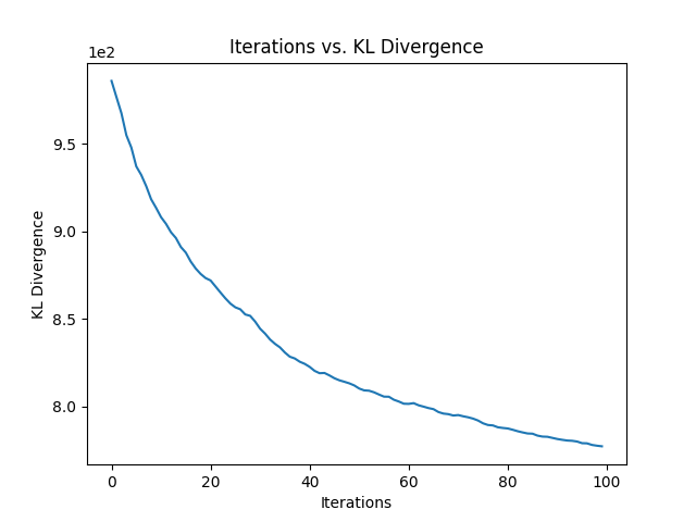
(a) With uniform start

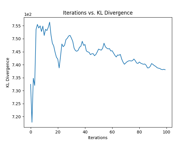
(b) No uniform start

Figure 3: Left: KL divergence over iterations with uniform start, Right: KL divergence over iterations without uniform start. They follow the same trajectory (except the erratic behavior at the beginning), but adding a uniform start greatly improves the stability of the algorithm and convergence.

Appendix B Algorithm

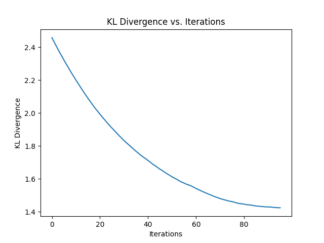
(a)

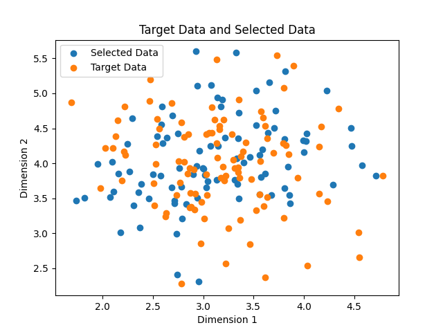
(b)

Figure 4: Sample plots for 2D example (Self-Consistency). Left: KL divergence over iterations, Right: Chosen data and target data

B.1 Usage

The code package for Gio is available on github at https://github.com/daeveraert/gradient-information-optimization. An example use in 2D (the self-consistency test, in this example):

⬇

from GIO import GIOKL

import numpy as np

import jax.numpy as jnp

import matplotlib.pyplot as plt

# Create some data

def getX():

mean = [3,4]

cov = [[0.5,0],[0,0.5]]

np.random.seed(1)

x, y = np.random.multivariate_normal(mean, cov, 100).T

return jnp.array([[x[i],y[i]] for i in range(len(x))])

def getXTest():

mean = [3,4]

cov = [[0.5,0],[0,0.5]]

np.random.seed(5)

x, y = np.random.multivariate_normal(mean, cov, 100).T

return jnp.array([[x[i],y[i]] for i in range(len(x))])

X = getX()

X_test = getXTest()

# Initialize class

gio_kl = GIOKL.GIOKL(uniform_low=0, uniform_high=8, \

uniform_start_size=100, dim=2)

# Perform the Algorithm

W, kl_divs, _ = gio_kl.fit(X_test, X, normalize=False)

W = W[100:] # Remove the uniform start

# Plot results

plt.plot(kl_divs)

plt.title("KL Divergence vs. Iterations")

plt.xlabel("Iterations")

plt.ylabel("KL Divergence")

plt.show()

plt.clf()

plt.scatter([each[0] for each in W], [each[1] for each in W], \

label="Selected Data")

plt.scatter([each[0] for each in X], [each[1] for each in X], \

label="Target Data")

plt.title("Target Data and Selected Data")

plt.xlabel("Dimension 1")

plt.ylabel("Dimension 2")

plt.legend()

plt.show()

The above code will print the KL divergence at each iteration and produce the plots in Figure 4.

A complex example using the quantization-explosion technique on big data with Spark:

⬇

from GIO import GIOKL

import jax.numpy as jnp

import matplotlib.pyplot as plt

import pyspark.sql.functions as F

# Initialize class

gio_kl = GIOKL.GIOKL(uniform_low=-1, uniform_high=1, uniform_start_size=20, dim=768)

# Read data

train_df, target_df = gio_kl.read_data_from_csv(PATH_TRAIN, PATH_TARGET)

# Quantize data

model_train, model_X, transform_train, transformed_X = \

gio_kl.quantize(train, target, k=1500)

X = jnp.array(model_X.clusterCenters())

train = jnp.array(model_train.clusterCenters())

data = [(i, each.tolist()) for i, each in \

enumerate(model_train.clusterCenters())]

centroids_df = gio_kl.spark.createDataFrame(data=data,\

schema=["id", "centroid"])

# Perform the Algorithm

W, kl_divs, _ = gio_kl.fit(train, X, max_iter=300, k=5, \

stop_criterion="sequential_increase_tolerance",\

v_init="jump",\

lr=0.01)

# Explode back to original data and write resulting data

full_selections_df = gio_kl.explode(W, centroids_df, transform_train)

full_selections_df.select(F.col("_c0"), F.col("_c1")).write \

.option("delimiter", "\t").csv(OUTPUT_PATH)

# Plot results

plt.plot(kl_divs)

plt.title("KL Divergence vs. Iterations")

plt.xlabel("Iterations")

plt.ylabel("KL Divergence")

plt.show()

The main function, GIOKL.fit, takes the following arguments:

• train: training data as a jnp array (jnp is almost identical to numpy) [M, D] shape

• X: target data as a jnp array [N, D] shape

• D: initial data as a jnp array, default None. Use None to initialize from 0 (uniform) or a subset of training data

• k: kth nearest neighbor to use in the KL divergence estimation, default 5

• max_iter: maximum iterations for the algorithm. One iteration adds one point (cluster)

• stop_criterion: a string for the stopping criterion, one of the following: 'increase', 'max_resets', 'min_difference', 'sequential_increase_tolerance', 'min_kl', 'data_size'. Default is 'increase'

  • min_difference: the minimum difference between prior and current KL divergence for 'min_difference'stop criterion only. Default is 0

  • resets_allowed: whether if KL divergence increases, resetting G to the full train is allowed (allows the algorithm to pick duplicates). Must be set to true if the stop criterion is 'max_resets'. Default is False

  • max_resets: the number of resets allowed for the 'max_resets'  stop criterion only (a reset resets G to the full train set and allows the algorithm to pick duplicates). Default is 2

  • max_data_size: the maximum size of data to be selected for the 'data_size'  stop criterion only, as a percentage (of total data) between 0 and 1. Default is 1

  • min_kl: the minimum kl divergence for the 'min_kl'stop criterion only. Default is 0

  • max_sequential_increases: the maximum number of sequential KL divergence increases for the 'sequential_increase_tolerance'  stop criterion only. Default is 3

• random_init_pct: the percent of training data to initialize the algorithm from. Default is 0

• random_restart_prob: probability at any given iteration to extend the gradient descent iterations by 3x, to find potentially better extrema. Higher values come at the cost of efficiency. Default is 0

• scale_factor: factor to scale the gradient by, or 'auto'. Default is 'auto', which is recommended

• v_init: how to initialize v in gradients descent, one of the following: 'mean', 'prev_opt', 'jump'. Default is 'mean'

• grad_desc_iter: the number of iterations to use in gradient descent. Default is 50

• discard_nearest_for_xy: discard nearest in the xy calculation of KL divergence, for use when X and the train set are the same, comes at the cost of efficiency. Default is False

• normalize: Whether to normalize the uniform start values. Use when the values of X and Train are normalized, as when using embeddings generated by MPNet or MiniLM, for example. Default is True

• lr: Learning rate for gradient descent. Default is 0.01

B.2 Stopping Criteria

We discuss several possible stopping criteria implemented in the code package and outline the pros and cons of each.

• Strict: The strictest stopping criterion (stopping_criterion="increase") is to stop immediately when the KL divergence increases from the previous value. This stopping criterion makes the most theoretical sense, as a KL divergence increase indicates the point being added does not add any information about the target X. This is the criterion we use for our text experiments. In practice however, it may be wise to allow some tolerance of KL divergence increase, which we discuss under the Sequential Increase Tolerance item.

• Convergence Tolerance: Closely related to the strictest stopping criterion is to specify a tolerance of the difference between the prior and current KL divergence and terminate when the difference falls below this tolerance (stopping_criterion="min_difference"). The tolerance is similar to tolerance arguments for gradient descent algorithms and is designed to heuristically identify when the algorithm has converged and is no longer decreasing by more than the specified amount.

• Minimum KL Divergence: The algorithm can terminate when it reaches a pre-determined KL divergence (stopping_criterion="min_kl"). In practice, however, it may be difficult to know beforehand what a good value of KL divergence may be, particularly in high dimensions.

• Maximum Data Size: The algorithm can terminate when it reaches a certain data size. This is a particularly useful stopping criterion when data size/resource constraints are the primary reason for data selection (stopping_criterion="max_data_size"). However, as it does not use intrinsic properties of the data that was selected (e.g. Kl divergence), it is the least theoretically-motivated stopping criterion. We use this stopping criterion for the FashionMNIST task in Section 4.4 (see Appendix C.5 for more details)

• Sequential Increase Tolerance: Instead of stopping when the KL divergence increases as in the strict criterion, we can allow the algorithm a certain amount of sequential increases in KL divergence before terminated. For example, a value of 3 would tell the algorithm to terminate after 3 consecutive points added each increased the KL divergence. If the KL divergence increases, then decreases again, the algorithm can continue. This criterion can allow the algorithm to attain better minima. Primarily, the space is non-convex, and allowing temporary increases in KL divergence can enable the algorithm to get over certain "humps" and descend into more ideal space. However, it could potentially lead to divergence in KL divergence, and also add many suboptimal points if KL divergence increases happen frequently or the tolerance is set too high.

Gio restricts points chosen to only be unique points. However, in some cases, allowing the algorithm to choose duplicate points can be beneficial. Intuitively, this would allow the algorithm to weight points in certain areas of the space it feels are most important. In practice, we can let the algorithm run until it reaches the chosen stopping criterion, then reset $G$ and allow the algorithm to pick again. We use this concept in our spelling correction experiments. In the code package, these options are given by the arguments resets_allowed (True or False) and max_resets, which specifies how many resets are allowed until full termination.

B.3 Initial v in Gradient Descent

We discuss the initial value of $\mathbf{v}$ in the gradient descent implemented in the code package and outline the pros and cons of each.

• Mean: The simplest initialization for $\mathbf{v}_{0}$ is to set it equal to the mean of the target $X$ at each iteration of Gio (v_init="mean"). This is motivated by the fact that the optimal $\mathbf{v}_{opt}$ lies somewhere in the space of $X$, and taking the mean will make $\mathbf{v}_{0}$ close to $X$ and is a good place to start searching. In unimodal symmetric distributions, the mean will essentially be the optimal point to add. In multimodal distributions, the mean provides a neutral starting point from gradient descent by which it can choose which mode to strike out for, based on the gradient. However, particularly in high dimensions, the mean may be far from the optimal point. Additionally, in scenarios where the modes are far apart and the distribution (and therefore the mean) is skewed to one section, starting from the skewed mean can miss the other sections of the space.

• Previous Optimal Point: We can also start $\mathbf{v}_{0}=\mathbf{v}_{opt}$, the previous optimal point found by gradient descent (v_init="prev_opt"). This is motivated by the fact that adding a new point is unlikely to alter the distribution much, and therefore the next optimal point is likely close to the previous optimal point. This is the setting we use in our text tasks. However in multimodal distributions with modes that are far apart, this may settle for only one or a few modes and not explore the rest of the space, as we are biasing the gradient descent to already-explored areas of the space. At the first iteration we can start from the mean.

• Random Jump: Instead of a deterministic starting point, we can set $\mathbf{v}_{0}$ to a random value from the target $X$ at each point in the iteration. This setting will explore various parts of the space, and algorithms better suited to non-convex spaces (e.g. particle swarm optimization (Kennedy and Eberhart, 1995)) also utilize stochastic methods as an instrument to achieve better convergence. Therefore, this setting can yield more diverse values and potentially better optima, with the risk of not being able to fully explore a particular area of the space. We use this technique in the FashionMNIST task, as in that task we know that the 10 classes of images will be multimodally distributed and the modes relatively delineated from each other, a setup which could cause issues with the previous two settings.

A combination of the methods, and additional methods, could perform even better and we leave this exploration to future work.

Appendix C Experiments

We provide the details of our experiments. All code to replicate experiments is included in the github repository (https://github.com/daeveraert/gradient-information-optimization), see Appendix B for details on usage.

C.1 Analytic Checks

We provide the sample code files to run the analytic checks in our code package at the path gradient-information-optimization/experiments/checks/:

• Self-Consistency: self_consistency.py

• Negative-Consistency: negative_consistency.py

• Quantization-Consistency: quantization_consistency.py

None of these code files require arguments, usage is python FILE.py. Figure 5 shows a visualization of the quantization consistency by plotting the estimated probability density functions of the original and quantized space. Figure 4 shows a visualization of self consistency by plotting the target and selected data.

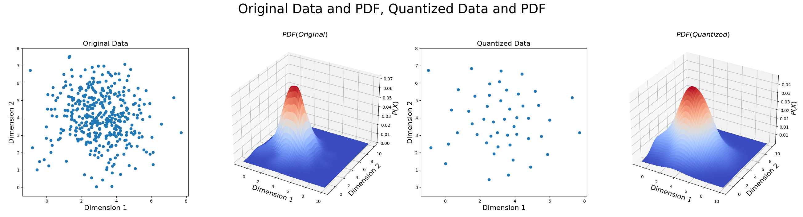
Figure 5: Visualization of quantization consistency. Left to right: Original data and kernel density-estimated PDF, Quantized data and kernel density-estimated PDF. The distributions are very close between the quantized space and original space.

C.2 WMT14

This experiment aims to demonstrate using Gio on a well-known dataset with a well-known setup, and shows Gio can achieve similar and even superior performance with significantly less data. See Section 4.1 for details on the results of this experiment. We follow Fairseq’s recommendations for replicating Vaswani et al. (2017) setup.

C.2.1 Data

We load and preprocess the data using https://github.com/facebookresearch/fairseq/blob/main/examples/translation/prepare-wmt14en2de.sh for EN-DE and https://github.com/facebookresearch/fairseq/blob/main/examples/translation/prepare-wmt14en2fr.sh for EN-FR. These scripts handle downloading, preprocessing, tokenizing and preparing the train, valid and test data. For our experiments, we combine the train and valid data from this to use in all of ours, competitive methods and random setups, and recut new validation sets for each experiment.

For the dev sets as our target $X$, we collect the dev sets for EN-FR and EN-DE from WMT08-WMT13 from the provided official dev sets of https://www.statmt.org/wmt14/translation-task.html and preprocess them using the same techniques and tokenizers given by the Fairseq processing scripts above. We then shuffle and cut 3k from the resulting combined dev sets to be used as our Dev Test set, and keep the remaining 12k as our target $X$.

C.2.2 Gio

We first generate embeddings for the train and dev sets using MPNet-Base-V2 (Song et al., 2020) on the input side of the data, using the following code from the code package:

⬇

from GIO import generate_text_embeddings

gen_embeds = generate_text_embeddings.GenerateEmbeddings("all-mpnet-base-v2")

gen_embeds.generate_embeddings(PATH_2_INPUT_SIDE_OF_DATA, OUTPUT_PATH)

We then paste the original "input \t output" with the embeddings file to create a file of the format "input \t output \t embedding" and use this as our CSV in Gio. We used AWS p3dn.24xlarge machines to generate the embeddings, which have 8 NVIDIA Tesla V100 GPUs and as a benchmark, takes roughly 4 hours to generate 15M embeddings (therefore approx. 8 hours for EN-FR and approx. 1 hour for EN-DE). This process is highly parallelizable for speed, and additionally, more lightweight models like MiniLM (which takes roughly half the time) and even non-neural methods like Sentence2Vec can be used under speed and resource constraints. Across all initializations, we use the following parameters:

• K: 1500

• k in $\mathbf{\hat{D}_{KL}}$: 5

• Max iterations: 1000

• Stopping Criterion: increase

• v_init: prev_opt

• Resets Allowed: false

• Iterations in Gradient Descent: 50

• Gradient Descent Learning Rate: 0.01

For 0% initialization, we use a uniform start of 20 points, spread from -1 to 1 with 768 dimensions. For 25% and 50% initialization, we start with a random subsample of 375 and 750 clusters respectively, out of the 1500. The following is the quantization and main method signatures for 0% initialization:

⬇

...

# Initialize class

gio_kl = GIOKL.GIOKL()

# Read data

train, target = gio_kl.read_data_from_csv(PATH_TRAIN, PATH_TARGET)

# Quantize data

model_train, model_X, transform_train, transformed_X = \

gio_kl.quantize(train, target, k=1500)

X = jnp.array(model_X.clusterCenters())

train = jnp.array(model_train.clusterCenters())

data = [(i, each.tolist()) for i, each in \

enumerate(model_train.clusterCenters())]

centroids_df = gio_kl.spark.createDataFrame(data=data,\

schema=["id", "centroid"])

# Perform the Algorithm

W, kl_divs, _ = gio_kl.fit(train, X, max_iter=1000, k=5, \

stop_criterion="increase",\

v_init="prev_opt",\

resets_allowed=False, grad_desc_iter=50,\

lr=0.01)

W = W[20:] # Remove uniform start

# Explode back to original data and write resulting data

full_selections_df = gio_kl.explode(W, transform_train, centroids_df)

full_selections_df.select(F.col("_c0"), F.col("_c1")).write \

.option("delimiter", "\t").csv(OUTPUT_PATH)

For 0% initialization, remove the variable D (both from when it is assigned to a random sample and from the main fit function call). For 50% initialization, increase 375 to 750.

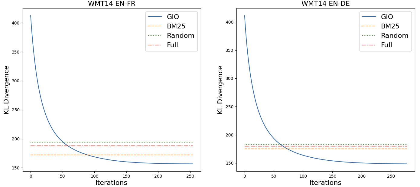
Figure 6: Gio surpasses the KL divergence of the most competitive baseline, BM25, at around 80 iterations and ends significantly lower

We performed this algorithm in a Spark environment on a cluster of 30 AWS r4.8xlarge CPU-only instances. For EN-DE, the algorithm took 40min end-to-end. For EN-FR, the algorithm took 50min end-to-end. We saved the initial K means quantized data for reuse in the different initialization states and during experimentation, which saves 10min for DE and 20min for FR on subsequent runs of the algorithm. In Figure 6, we show the KL divergence graphs over the iterations for EN-FR and EN-DE at 0% initialization, and include lines indicating the divergence for BM25, Pruning, Submodular Optimization, Random and Full baselines.

C.2.3 Baselines

For the random baselines, after running Gio, we take a random sample of the same size as that chosen by Gio. For BM25, we also select sample of the same size as that chosen by Gio. Yao et al. (2022) provide a Github implementation of their data selection technique at https://github.com/yaoxingcheng/TLM (Yao and Zhang, 2021). We use the data_selection.py, for example:

⬇

python src/data_selection.py \

--index_name example_bm25_source \

--source_file SOURCE.csv \

--target_file TARGET.csv \

--output_dir ./example_data \

--output_name selected.csv \

--top_k K

The source file is the (input only) data we can select from, $G$, and the target file is the (input only) $X$, in this case the collected dev sets. Top K is the parameter that tells BM25 how much data to retrieve for each data point in $X$. Since BM25 can output a score of 0 and discard data, we cannot calculate K as $K=\frac{|G|}{|X|}$, and typically, we need to overestimate K to collect enough data to match the desired size. We also need to pre and post process our data to conform to their code, which we address and provide scripts for.

Preproccessing.

Their implementation requires a CSV with columns text,id, but data given to us with the WMT14 scripts is in plain text format with no ID. We provide a script at gradient-information-optimization/experiments/bm25_scripts/make_csv.py which transforms a single-column file of inputs into the format needed by the Yao et al. (2022) code:

⬇

python make_csv.py INPUT_FILE TO_OUTPUT_FILE

Postprocessing.

Their implementation will output a CSV with the format chosen_data,input ID,rank. The rank is the value of "K" for which this data was retrieved. For example, if this was the 5th most relevant to a data point, then the rank will read 5. As addressed, we need to overestimate K to collect enough samples. Inevitably, we end up with too many samples, and need to trim down the data by removing the least relevant retrievals. We provide a script at gradient-information-optimization/experiments/bm25_scripts/get_less.py which takes in the file output by their code, an output path, and a value of rank to filter; we keep the values under the specified rank value, and discard any over. This is a trial-and-error process, repeatedly trying different values of K until we get the desired data size. Usage is:

⬇

python get_less.py INPUT_FILE TO_OUTPUT_FILE K_FILTER_VALUE

Finally, we need to recover the input-output pairs, as the output file only has input-side data. We provide a script at gradient-information-optimization/experiments/bm25_scripts/get_pairs.py that retrieves the pairs from input side given the input data and original data of the format input \t output:

⬇

python get_pairs.py ORIGINAL_DATA INPUT_FILE TO_OUTPUT_FILE

For submodular optimization, we use the same cluster centers as Gio, the LazyGreedy optimizer and facility location mutual information function, and run to have the same data size as the Gio-selected data. We provide a script at gradient-information-optimization/experiments/submod/submod.py which takes three inputs and an output argument. The first input should be a parquet file with one column of array<double> for the data and the second input should be the same for the target $X$. The third input should be the threshold data size, determined by $\frac{\text{Desired Data Size}}{\text{Total Data Size}}\cdot\text{Cluster Size}$, and the output should also be a parquet file with a column array<double>.

⬇

python submod.py DATA_CLUSTERS X_CLUSTERS THRESHOLD TO_OUTPUT_FOLDER

For self-pruning, we use the same cluster centers as Gio. We adapt their technique in gradient-information-optimization/experiments/pruning/prune.py which takes three inputs and one output argument. The first input should be a parquet file of the cluster centers and the second input should be the transformed dataframe from Spark’s KMeans. The third input should be the threshold, which is calculated by the formula $\frac{\text{Desired Data Size}}{\text{Cluster Size}}$. The output should be output folder.

⬇

python prune.py INPUT_CLUSTERS TRANSFORMED_DF THRESHOLD TO_OUTPUT_FOLDER

C.2.4 Training

We preprocess and train using Fairseq (Ott et al., 2019). We cut 3k pairs from the data for validation and keep the rest as training data. We use the subword-nmt package to apply BPE Sennrich et al. (2016), Sennrich (2021) using the codes already computed and provided by the Fairseq scripts to download data (Appendix C.2.1). We then use fairseq-preprocess to preprocess the data into Fairseq-readable format. We then follow the Vaswani et al. (2017) setup and train for 300k iterations, saving every 15k iterations. We use Fairseq’s pre-built transformer_vaswani_wmt_en_fr_big architecure for EN-FR and transformer_vaswani_wmt_en_fr_big for EN-DE. The pre-built architectures preset essentially all of the model parameters described by Vaswani et al. (2017). We followed the recommendation in https://github.com/facebookresearch/fairseq/issues/346 to set the LR at 0.0007 for close replication of Vaswani et al. (2017) with the Fairseq framework. We varied the max_tokens parameter to ensure approximately 25k tokens per batch, as recommended in the paper (Vaswani et al., 2017).

EN-FR CLI

⬇

$(which fairseq-train) DATA_PREPROCESSED \

--arch transformer_vaswani_wmt_en_fr_big \

--share-all-embeddings \

--optimizer adam --lr 0.0007 \

--dropout 0.1 \

--max-tokens 3512 \

--lr-scheduler inverse_sqrt --weight-decay 0.0 \

--criterion label_smoothed_cross_entropy --label-smoothing 0.1 \

--fp16 --save-dir SAVE_DIR --save-interval-updates 15000 \

--max-update 300000 --clip-norm 0.0 --warmup-updates 4000 \

--warmup-init-lr 1e-07 --min-lr 1e-09 --adam-betas ’(0.9,0.98)’

EN-DE CLI

⬇

$(which fairseq-train) DATA_PREPROCESSED \

--arch transformer_vaswani_wmt_en_de_big \

--share-all-embeddings \

--optimizer adam --lr 0.0007 \

--dropout 0.3 \

--max-tokens 3512 \

--lr-scheduler inverse_sqrt --weight-decay 0.0 \

--criterion label_smoothed_cross_entropy --label-smoothing 0.1 \

--fp16 --save-dir SAVE_DIR --save-interval-updates 15000 \

--max-update 300000 --clip-norm 0.0 --warmup-updates 4000 \

--warmup-init-lr 1e-07 --min-lr 1e-09 --adam-betas ’(0.9,0.98)’

We trained on one AWS p3dn.24xlarge, which has 8 NVIDIA Tesla V100 GPUs and takes about 10 hours to train the full 300k iterations.

C.2.5 Testing

We use the script provided by Fairseq moderators in https://gist.github.com/myleott/da0ea3ce8ee7582b034b9711698d5c16 (Ott, 2019) for the evaluation process. In order to generate the predictions on the preprocessed test data from the best model by validation loss, we use the checkpoint_best.pt model produced by Fairseq and the command:

⬇

fairseq-generate TEST_DATA --path MODEL --beam 4 --lenpen 0.6 \

--remove-bpe > outfile

The outfile then gets fed into the script provided by the Fairseq moderators to give the BLEU score.

C.3 Robustness

The robustness experiments follow a nearly identical setup to the above WMT14 setup. We outline the differences:

MiniLM.

To use MiniLM to generate the embeddings for Gio, we replace "all-mpnet-base-v2" with "all-MiniLM-L12-v1" in the GenerateEmbeddings class instantiation:

⬇

from GIO import generate_text_embeddings as gte

gen_embeds = gte.GenerateEmbeddings("all-MiniLM-L12-v1")

gen_embeds.generate_embeddings(PATH_2_INPUT_SIDE_OF_DATA, OUTPUT_PATH)

MiniLM takes roughly half the time than MPNet to generate embeddings. On an AWS p3dn.24xlarge machine with 8 NVIDIA Tesla V100 GPUs, it takes roughly 30min for EN-DE and roughly 4 hours for EN-FR. In addition, we alter the instantiation of the GIOKL class to specify dimensions of 384:

⬇

...

gio_kl = GIOKL.GIOKL(dim=384)

...

All else stays the same as the WMT14 setup.

K=1000 and K=3000.

For the experiments altering the value of K, we reuse all the embeddings generated with MPNet for the main experiments. The only difference is to the quantize method signature with the difference values of K:

⬇

...

model_train , model_X , transformed_train , transformed_X = \

gio_kl.quantize(train, target , k=1000) # Or k=3000

...

All else stays the same as the WMT14 setup.

When computing the variance from the base setup for data size, we omit the K=1000 data size since (as covered in Section 4.2) we need to artificially subsample to keep the selected data size the same as in the base setup. This is due to the coarser grain of K=1000 selecting more data. Interestingly, K=3000 and MiniLM selects roughly the same data as the base setup.

C.4 Speller

This experiment aims to demonstrate using Gio on a mix of high and low quality data, and aims to show Gio selects the high quality data. We use the spelling correction domain for this problem, as the process of noising training data to create training pairs makes it easy to create high and low quality synthetic data by varying the noise. We determine the % of high quality data selected by each method, and also train a model and show spelling performance of our method, random subset, BM25, pruning and submodular optimization and show the results of Gio-selected data are better than that trained on the full mix of low and high quality data Table 6. We generally follow the recent work of Jayanthi et al. (2020) for this problem.

C.4.1 Data

Jayanthi et al. (2020) use the 1 Billion Word Corpus and extract roughly 1M pairs for creating synthetic data. In order to show our method at scale, we download the full 1 Billion Word Corpus from https://www.statmt.org/lm-benchmark/ and extract 15M data. We add in the 1M pairs used by Jayanthi et al. (2020) and deduplicate on label, which results in roughly 14.7M data. When we have the labels, we need to noise them to create the inputs. Jayanthi et al. (2020) implement and use 3 different synthetic data noising methods: random, word and prob. They show "prob" is the best method, followed by "word" and then "random". We use the "prob" method on half the data to create our high quality input-output pairs, and use the "word" method on the remaining half. The "word" method takes in a probability that a word will be replaced by a misspelled version of it contained in a lookup table, if it exists. Jayanthi et al. (2020) use a probability of 20%, but to make very low quality data, we use a high probability of 70%. They provide a Github implementation of their methods and data at https://github.com/neuspell/neuspell (Jayanthi, 2021), which we use to noise the data accordingly. We give an example of the quality difference in Table 5.

Table 5: Right: High Quality "Prob" data. Left: Low Quality "Word" data. High quality data represents reasonable spelling mistakes, low quality data is barely intelligible. Gio selects 73% from the high quality data.

High Quality "Prob"	Low Quality "Word"
It is still a big poblem though	It ls sttel a beig probelma thouigh
It apoeared they were not serousay injured , the BBC said	It appered thiy whir nt serioulsly ingerd , whe BBC sayd
Were they aarried on Feb	Were thwey marreid ong Feb
More of us are tuning in to tha irwaves than ever	More th uus spe tuning inf tome vthe airwaves thanx ef

The high quality "prob" data is more reflective of real spelling mistakes, and in fact the "prob" method uses a context matrix to make applicable misspellings in context. The "word" method at 70%, on the other hand, severely mangles the sentences to the point where we barely make out what they mean, making for very low quality data to train with. After generating half with prob and half with word, we recombine and shuffle to create our training data. For our target $X$ set, Jayanthi et al. (2020) provide 40k pairs of real mistakes by humans taken from the BEA grammar correction corpus (Bryant et al., 2019), which we use as our ideal target $X$.

C.4.2 Gio

We first generate embeddings for the train and target sets using MPNet-Base-V2 (Song et al., 2020) on the input side of the data; see Appendix C.2 for an example, we use the same process as in our WMT experiments. On an AWS p3dn.24xlarge machine with 8 NVIDIA Tesla V100 GPUs, it takes about 4 hours to generate the embeddings for the 15M data. As we mention in Section 4.3, we experiment with a new scheme. Instead of stopping on an increase, we allow the algorithm to reset $G$ once when the KL divergence increases, and pick again until the divergence increases a second time. We hope this will allow the algorithm to pick not only high quality data, but emphasize (by picking duplicates) the points that are also the most relevant for $X$. We use the following parameters in the algorithm:

• K: 1500

• k in $\mathbf{\hat{D}_{KL}}$: 5

• Max iterations: 1000

• Stopping Criterion: increase

• v_init: prev_opt

• Resets Allowed: True

• Maximum Resets: 1

• Iterations in Gradient Descent: 50

• Gradient Descent Learning Rate: 0.01

The method is as follows:

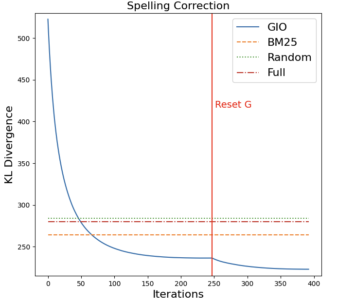
Figure 7: Resetting G enables the algorithm to make further progress reducing KL divergence.

⬇

...

# Initialize class

gio_kl = GIOKL.GIOKL()

# Read data

train, target = gio_kl.read_data_from_csv(PATH_TRAIN, PATH_TARGET)

# Quantize data

model_train, model_X, transform_train, transformed_X = \

gio_kl.quantize(train, target, k=1500)

X = jnp.array(model_X.clusterCenters())

train = jnp.array(model_train.clusterCenters())

data = [(i, each.tolist()) for i, each in \

enumerate(model_train.clusterCenters())]

centroids_df = gio_kl.spark.createDataFrame(data=data,\

schema=["id", "centroid"])

# Perform the Algorithm

W, kl_divs, _ = gio_kl.fit(train, X, max_iter=1000, k=5, \

stop_criterion="increase",\

resets_allowed=True, max_resets=1, \

v_init="prev_opt", grad_desc_iter=50,\

lr=0.01)

W = W[20:] # Remove uniform start

# Explode back to original data and write resulting data

full_selections_df = gio_kl.explode(W, transform_train, centroids_df)

full_selections_df.select(F.col("_c0"), F.col("_c1")).write \

.option("delimiter", "\t").csv(OUTPUT_PATH)

We performed this algorithm in the same Spark environment on a cluster of 30 AWS r4.8xlarge CPU-only instances, which took around 1h15m to complete. In Figure 7, we show the KL divergence graphs over the iterations and include lines indicating the divergence for BM25, Pruning, Submodular Optimization, Random and Full baselines. We mark where the algorithm reset $G$; we can see the KL divergence further decreases.

C.4.3 Baselines

For the random baseline, after running Gio, we take a random sample of the same size as that chosen by Gio. For BM25, submodular optimization and pruning, please see Appendix C.2.3, as we follow exactly the same process as in our WMT experiments, using the same scripts but on different data. We also train a model on the full data for comparison.

C.4.4 Training

We preprocess and train using Fairseq (Ott et al., 2019). We cut 3k pairs from the data for validation and keep the rest as training data. We use the subword-nmt package (Sennrich, 2021) to learn and apply a 40k BPE from the combined source and target data. We then use fairseq-preprocess to preprocess the data into Fairseq-readable format. We train with a seq2seq setup proposed by Zhou et al. (2019) that learns to map input (noised) to output labels (regular, no noise). We use the BART base architecture (Lewis et al., 2020) as our seq2seq model, since the denoising objective they used when developing BART is naturally suited to the spelling correction task. We train for 50k iterations and pick the best model checkpoint by validation loss, saving every 5000 iterations. We use 4096 max tokens per batch, the Adam (Kingma and Ba, 2015) optimizer with LR of 0.0001, and generally keep the rest of the settings the same as in the BART paper (Lewis et al., 2020). For our method and all baselines, we train twice and take the average.

Speller CLI

⬇

$(which fairseq-train) DATA_PREPROCESSED \

--arch bart_base \

--share-all-embeddings \

--optimizer adam --lr 0.0001 \

--dropout 0.1 \

--max-tokens 4096 \

--lr-scheduler inverse_sqrt \

--fp16 --save-dir SAVE_DIR --save-interval-updates 5000 \

--max-update 50000 --clip-norm 0.0 --warmup-updates 4000 \

--warmup-init-lr 1e-07 --min-lr 1e-09 --adam-betas ’(0.9,0.98)’

We trained on one AWS p3dn.24xlarge, which has 8 NVIDIA Tesla V100 GPUs and takes about 2 hours to train the full 50k iterations.

C.4.5 Testing

As test data, Jayanthi et al. (2020) provide several sets. We cannot use the BEA 60k they provide as we used 40k from this as our target $X$. Instead, Jayanthi et al. (2020) provide an even more challenging set of 4660 intentionally ambiguous pairs curated from BEA60k (the 4660 pairs have no overlap with our $X$), and we use this test set. We tokenize and preprocess this test set with the same codes as our training data. For metrics, Jayanthi et al. (2020) report word-level accuracy and word-level correction rate. Word-level accuracy is the fraction of words that the model gets correct, and word-level correction rate is the fraction of words that should be corrected that do get corrected. We also report the F1 score as a balance between these two metrics. In theory it is possible to arbitrarily correct every single word randomly and get 100% correction rate but 0% accuracy, or keep every word the same and get near 100% accuracy but 0% correction rate.

An additional complexity arises with our particular use of a seq2seq framework. The models of Jayanthi et al. (2020) use a classification objective to classify each input word, which means the output and input sequence will mandatorily have the same number of words. However, this property is not necessarily guaranteed for a seq2seq setup with subword tokenization, and after inferencing our models on test data we see a small number (roughly 1%) where the input and output number of words do not match. For fairness, when evaluating the models we remove the few sequences that have a misalignment from the evaluation. In order to generate the predictions on the preprocessed test data from the best model by validation loss, we use the checkpoint_best.pt model produced by Fairseq and the command:

⬇

fairseq-generate TEST_DATA --path MODEL --beam 1 \

--remove-bpe > outfile

grep ^H outfile | cut -f3- > hypotheses

grep ^T outfile | cut -f2- > targets

grep ^S outfile | cut -f2- > sources

We then feed the hypotheses, targets and sources into a script we provide at gradient-information-optimization/experiments/speller_scripts/calculate_scores.py which computes the word-level accuracy and correction rate.

Table 6: Spelling correction results. Training data size, accuracy/correction rate/F1 scores, % of high quality data and KL Divergence of the full data, the Gio-selected data, competitive methods and random subset. Bold is the best score overall. Gio selects 73% high quality data, outperforms all other methods and sets a new state-of-the-art on spelling correction.

System	Train Size	Accuracy	Correction Rate	F1	%High Quality	$\mathbf{\hat{D}_{KL}}$
Ours		95.9	99.6	97.7	73%	224
BM25		95.6	99.3	97.4	55%	264
Pruning	03.6M	95.7	99.6	97.6	54%	-
Submod.		95.7	99.5	97.6	59%	245
Random		95.9	99.4	97.6	50%	284
Full	14.7M	95.7	99.5	97.6	50%	280

Results

Gio outperforms random, all comparative methods, and the full model. Gio outperforms all comparative baselines on accuracy, correction rate and overall F1, and matches random baseline on accuracy and outperforms on correction rate and overall F1. It outperforms the full model by +0.2pps for accuracy and +0.1pps for correction rate, despite using only 24% of the data. We set a new state-of-the-art in correction rate and overall F1 score on BEA4660 over the best model reported by Jayanthi et al. (2020) (+2.3 pps F1 and +7.2 pps correction rate). See Table 6 for details.

C.5 FashionMNIST

This experiment aims to demonstrate using Gio can effectively reduce the training data size under a resource constraint without big drops in performance. We use the FashionMNIST image recognition task (Xiao et al., 2017) to demonstrate using Gio outside language tasks. Our goal is to reduce the train set size to 25% of the total size. Experiment results are available at Section 4.4.

C.5.1 Data

The FashionMNIST task has 60k 28x28x1 images for training and 10k images for testing. We load the images in CSV format from https://www.kaggle.com/datasets/zalando-research/fashionmnist (Pankaj, 2019). In our dataloader, we resize our images to 224x224 for Resnet50 using skimage’s resize function, normalize each channel, and additionally normalize the values to fall within 0 and 1. The dataloader code is available in the main file we publish at gradient-information-optimization/experiments/fashion_mnist/train.py. We based the dataloader code on code provided at https://www.kaggle.com/code/pankajj/fashion-mnist-with-pytorch-93-accuracy. We use the vector format of the images themselves in Gio. $G$ is the training set, but in this case, $X$ is also the training set. Since our goal is to reduce the training set size, we want to select a subset of $G$ that contains the most information about the whole set, so the target set is the whole set itself.

C.5.2 Gio

In order to read the images using the code package, we do a simple processing to make the image CSV into a string representing an array, the script is available at gradient-information-optimization/experiments/fashion_mnist/csv_to_image.py; first argument is input, second is output. We also normalize each channel and norm each image. For the algorithm itself, we stop at 25% data size, and use K=1000. With this problem, we know that there are 10 classes and the images are likely to be clustered relatively distinctly, by class. Therefore, for the initial $\mathbf{v}$ in gradient descent, we choose the random jump scheme, as we will therefore be able to cover more of the space. We use the following parameters in the algorithm:

• K: 1000

• k in $\mathbf{\hat{D}_{KL}}$: 5

• Max iterations: 300

• Stopping Criterion: data_size

• Maximum Data Size: 0.25

• v_init: jump

• Iterations in Gradient Descent: 50

• Gradient Descent Learning Rate: 0.01

The method is as follows:

⬇

...

# Initialize class

gio_kl = GIOKL.GIOKL()

# Read data

train, target = gio_kl.read_data_from_csv(PATH_TRAIN, PATH_TARGET)

# Quantize data

model_train, model_X, transform_train, transformed_X = \

gio_kl.quantize(train, target, k=1000)

X = jnp.array(model_X.clusterCenters())

train = jnp.array(model_train.clusterCenters())

data = [(i, each.tolist()) for i, each in \

enumerate(model_train.clusterCenters())]

centroids_df = gio_kl.spark.createDataFrame(data=data,\

schema=["id", "centroid"])

# Perform the Algorithm

W, kl_divs, _ = gio_kl.fit(train, X, max_iter=300, k=5, \

stop_criterion="data_size",\

max_data_size=0.25, v_init="jump", \

resets_allowed=False, grad_desc_iter=50,\

lr=0.01)

W = W[20:] # Remove uniform start

# Explode back to original data and write resulting data

full_selections_df = gio_kl.explode(W, transform_train, centroids_df)

full_selections_df.select(F.col("_c0"), F.col("_c1")).write \

.option("delimiter", "\t").csv(OUTPUT_PATH)

We performed this algorithm in the same Spark environment on a cluster of 30 AWS r4.8xlarge CPU-only instances, which took around 20m to complete. We show the KL divergence over the iterations. In this case, the minimum KL divergence is not 0, but 739. We explain why the KL divergence is not 0 in Appendix A.1. The graph of KL divergence is shown in Figure 8.

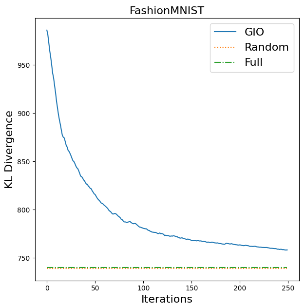
Figure 8: Gio approaches the KL divergence of the full data

Baselines.

For the random baseline, after running Gio, we take a random sample of the same size as that chosen by Gio. We also train a model on full data for comparison, but the goal in this setup is not to match or exceed the full model, but minimize the drop in performance under the resource constraint.

C.5.3 Training and Testing

We finetune a pretrained Resnet50 model with the data. For Gio and random, we cut 1,700 as validation and leave the remaining 15,000 (25%) as our training data. For the full model, we follow this percentage and cut 3,700 as validation and keep 56,300 as the training data. In order to get the images back into the correct CSV format for the dataloader from a string-array format, we provide a script at gradient-information-optimization/experiments/fashion_mnist/image_to_csv.py; first argument is input, second is output. We edit the architecture of the Resnet50 model on the input layer to take 1 channel instead of 3, and edit the output layer to output to 10 classes. We finetune for 5 epochs with Adam and a small learning rate of 0.00005 so as not to overwrite the existing weights in the pretrained model. We use batch size 100 and take the best checkpoint by validation loss and report the test score on this. The code to read and train a model is available at gradient-information-optimization/experiments/fashion_mnist/train.py. We based this training script on code provided at https://github.com/kjamithash/Pytorch_DeepLearning_Experiments/blob/master/FashionMNIST_ResNet_TransferLearning.ipynb (J, 2020). Usage:

⬇

python train.py TRAIN_CSV TEST_CSV VALID_CSV

For testing, the above code will output the test accuracy at each epoch. We train on one AWS p3dn.24xlarge machine, which has 8 NVIDIA Tesla V100 GPUs and takes around 15min to train.

Appendix D Further FashionMNIST

D.1 Gio KL Divergence vs. Random KL Divergence

It is interesting that despite achieving a higher KL divergence than the random baseline, Gio performs better. We hypothesize that this is due to the fact that Gio is optimizing explicitly for choosing images that add the most information about the whole, i.e., discarding outlier data and focusing on "core" data under the size constraint, which leads to higher KL divergence than random but better performance, as the model will be less confused. For example, in the "bag" category, conceivably a good portion of the bags look very similar, but there is also a portion that are more strange. Random would choose both the core portion of bags that looks similar but also include some of the stranger examples. Gio, on the other hand, will focus almost exclusively on choosing the core portion, as that is the set that adds the most information, or best represents, the bag category overall. In short, outliers are less important to know under a size constraint, and the core is more important to get right, which Gio chooses. We validate this hypothesis in three ways.

2D Embeddings.

First, we perform a tSNE dimensionality reduction on the random set and Gio set in Figure 9. The diagrams show that Gio selects more core, densely clustered data and leads to better separability between classes. It does not choose much outlier data for each class that is spread around the space and could confuse the model. Random, on the other hand, is generally less separable and more sparse, and includes potentially confusing points in each class that are spread around the space and overlapping with other classes, which could confuse the model. In short, Gio-selected data is more dense and separable than random and is likely to lead to better classification performance, but will have higher KL divergence from full data than the random data because of this effect on the distribution.

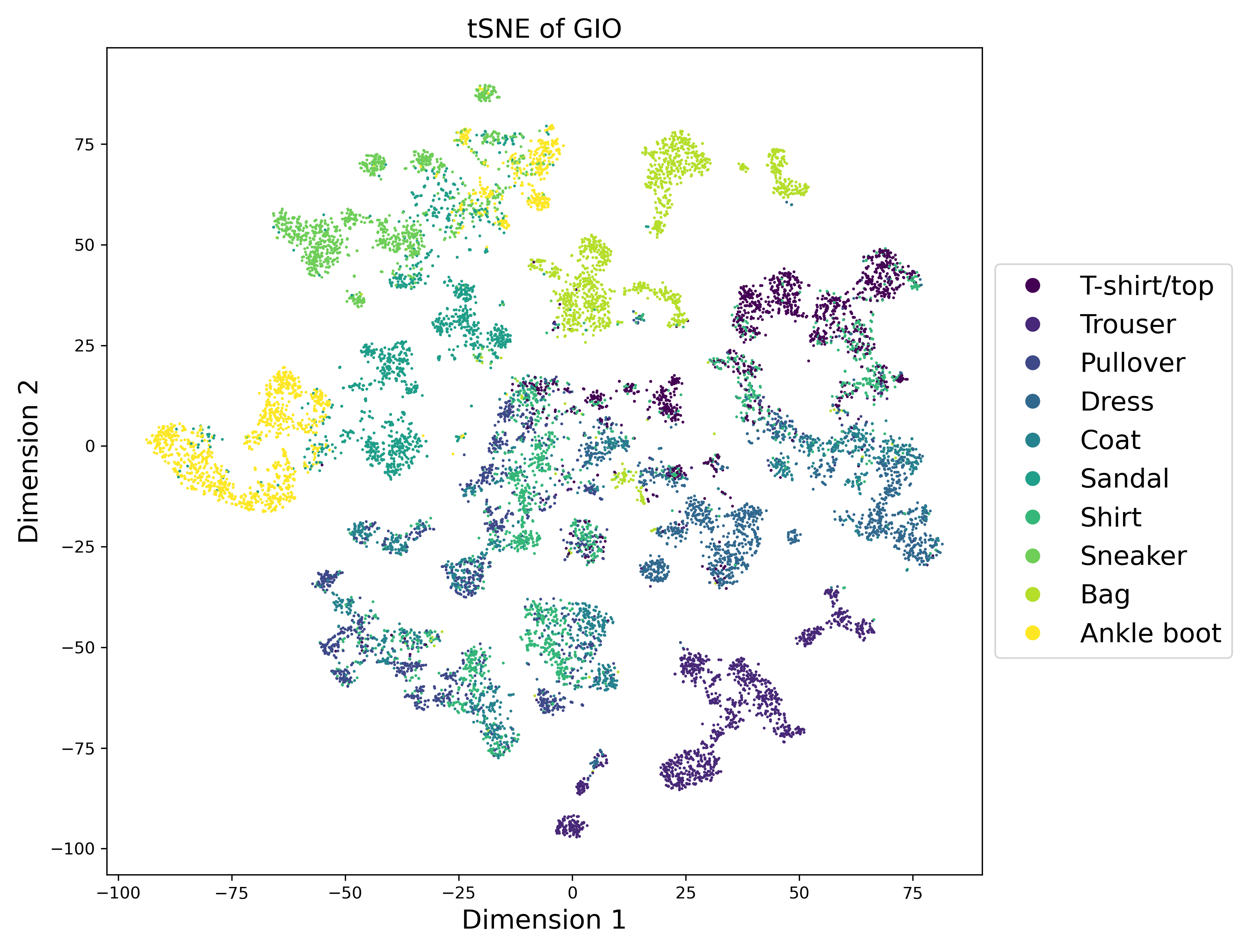
(a)

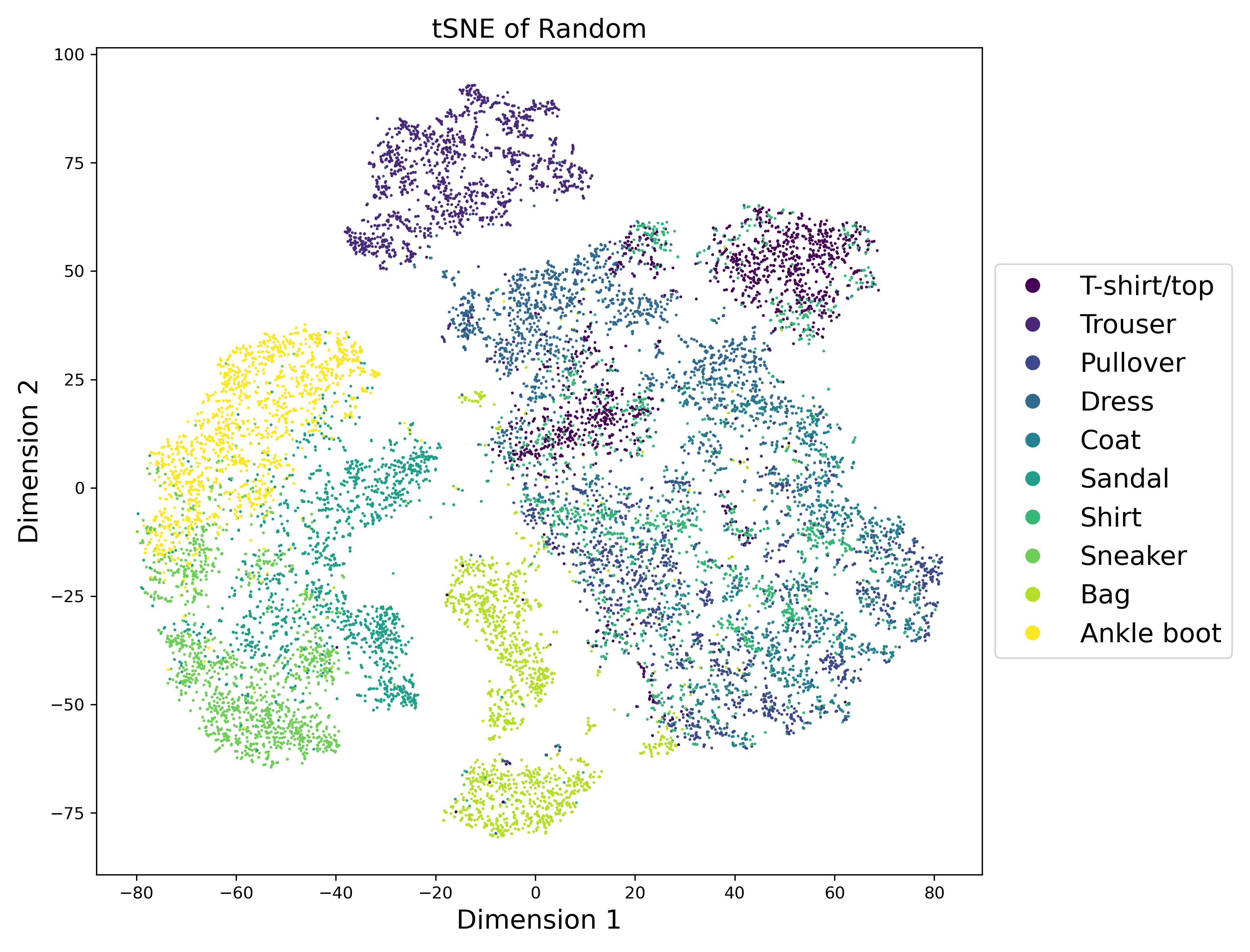
(b)

Figure 9: Left: tSNE of Gio, Right: tSNE of Random. Gio is more separable and dense in each class, indicating Gio chooses more core data and fewer outliers

(a)

(b)

Figure 10: Left: Chosen "Bag" images of Gio, Right: Chosen "Bag" images of Random. Rectangular shaped bags form the core of the full bag class (by visual inspection). The bags chosen by Gio are consistent and similar, and are all rectangular in shape and similar sizes. Random bags, however, also include a variety of more uncommon outlier shapes, including a tote bag and triangular bag. Under a data constraint, it is more important to get the core rectangular bag correct, as Gio chooses.

Visualization.

As an additional sanity check, we visually inspect the images chosen by Gio and random images in Figure 10. We show the bag class as an example. Gio selects more consistent bags that conform to each other. They are all rectangular and similar in size, and represent the core set of bag images, as regular rectangular bags form most of the class (as determined by visualizing samples from the full set). Random images, on the other hand, contain more strange images like triangular bags and tote bags and are less consistent. Under a data constraint, Gio focuses on the core rectangular bags that best represent the class and discards outliers, which leads to better performance.

Separability.

Finally, we examine the separability between classes as an indicator of whether Gio selects images that are more core and less spread/confusing. We compute the Euclidean mean for each class and compute the average distance of that mean to the means of all other classes, for Gio-selected data and random images. Table 7 shows the results, and demonstrates that Gio classes are further away from each other in every class. This implies Gio selects more distinct and less confusing points, and likely explains the improved classification performance over random images.

Table 7: Mean Euclidean distance between the mean of each class and the means of all other classes. Higher is better, as it indicates the class is further apart from others and therefore more separable. Gio is higher in every class, indicating Gio-selected data is more separable than random images.

Class	Gio	Random
0	2469	2383
1	2500	2451
2	2482	2447
3	2380	2360
4	2475	2442
5	2733	2649
6	2321	2294
7	2614	2550
8	2674	2667
9	2774	2696

D.2 Label Distribution

One of the core assumptions of the method is that we can utilize only the input side of data without consideration for labels. By reconstructing an approximate $X$ using $G$ with only the input side, we implicitly reconstruct the label side of $X$ as well, and therefore there is no need to consider the labels explicitly. We verify this assumption with FashionMNIST, as it has distinct, quantifiable labels unlike the text generation tasks. Table 8 shows the distribution of labels recovered by Gio, and shows that we approximately recover an even 10% for each class, which is the distribution of the full $X$. Therefore, Gio recovers the distribution of labels in $X$ implicitly, despite not including them in the algorithm, as desired. This is not to say labels are not important in data selection. We note that for the algorithm to work well, there should exist a quality relation between input and label. Specifically, we require that either input and label are good quality, or input and label are bad quality. If a good quality input maps to a wrong or bad quality label, we may recover bad labels.

Table 8: Distribution of labels per class. Despite only considering inputs, Gio also recovers the label distribution of the target $X$.

Class	0	1	2	3	4	5	6	7	8	9
% of Total	9.9%	9.3%	9.3%	10.8%	10.5%	9.6%	12.2%	8.2%	10.1%	10.4%

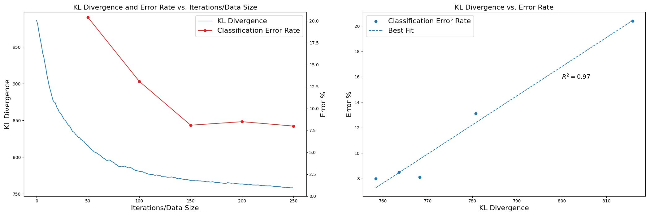
Figure 11: Left: KL divergence and Classification Error Rate over different data sizes. The shape of the two curves are very similar. Right: KL divergence and Classification Error Rate. High $R^{2}=0.97$ indicates Kl divergence can accurately predict performance.

Table 9: Performance of the model using the different datasizes chosen as the algorithm progresses.

Iterations/Data %	Size Train/Valid	Accuracy	$\mathbf{\hat{D}_{KL}}$
50/5%	3,200/200	79.6%	816
100/10%	6,000/400	86.9%	781
150/15%	9,100/600	91.9%	768
200/20%	12,500/900	91.5%	764
250/25%	15,000/1,700	92.0%	759

D.3 Correlation Between Performance and KL Divergence

We know that under the FashionMNIST problem setup for reducing training set size, a data size was chosen beforehand, which in practice would represent a budget. However, beyond budget concerns, we endeavored to find out if we could use the KL divergence to predict what a good, convergent data size would be. Perhaps 25% is more than enough and we could do just as well with less, or perhaps 25% is too little to get good performance, and we might want to increase our resources before experimenting. In this setup, we know the KL divergence values at each data size (each iteration), and we want to see whether the shape of the KL divergence curve could indicate the shape of the performance curve at the different data sizes. We repeat the same experiment described in Section 4.4, but using 50 iterations (5% data), 100 iterations (10% data), 150 iterations (15% data) and 200 iterations (20% data). We plot the results of both KL divergence and performance (classification error rate) in Figure 11 and describe the results in Table 9. In Figure 11, we additionally plot error rate as a function of KL divergence and compute the coefficient of determination $R^{2}$. We find that the shape of classification error vs. data size and KL divergence vs. data size are very similar. Additionally, $R^{2}=0.97$, which indicates a high degree of correlation between KL divergence with data size and performance. Theoretically, this implies that we can use the KL divergence to pick an ideal data size if we are under budget constraints: where the KL divergence curve flattens, we are unlikely to receive much gain in performance from increasing the data size further and can use that data size with the expectation of decent performance. We only have a few datapoints to support this hypothesis, however, and we leave exploration of this property of the algorithm to future work.

References

- Arthur and Vassilvitskii (2007) David Arthur and Sergei Vassilvitskii. k-means++: the advantages of careful seeding. In SODA ’07: Proceedings of the eighteenth annual ACM-SIAM symposium on Discrete algorithms, pages 1027–1035. Association for Computing Machinery, January 2007. doi: 10.5555/1283383.1283494. URL https://dl.acm.org/doi/10.5555/1283383.1283494.
- Bernhardsson (2017) Erik Bernhardsson. Annoy (approximate nearest neighbors oh yeah), 2017. URL https://github.com/spotify/annoy. Apache-2.0 license.
- Brown et al. (2020) Tom B. Brown, Benjamin Mann, Nick Ryder, Melanie Subbiah, Jared Kaplan, Prafulla Dhariwal, Arvind Neelakantan, Pranav Shyam, Girish Sastry, Amanda Askell, Sandhini Agarwal, Ariel Herbert-Voss, Gretchen Krueger, Tom Henighan, Rewon Child, Aditya Ramesh, Daniel M. Ziegler, Jeffrey Wu, Clemens Winter, Christopher Hesse, Mark Chen, Eric Sigler, Mateusz Litwin, Scott Gray, Benjamin Chess, Jack Clark, Christopher Berner, Sam McCandlish, Alec Radford, Ilya Sutskever, and Dario Amodei. Language models are few-shot learners. arXiv preprint arXiv:2005.14165, 2020.
- Bryant et al. (2019) Christopher Bryant, Mariano Felice, Øistein E. Andersen, and Ted Briscoe. The BEA-2019 shared task on grammatical error correction. In Proceedings of the Fourteenth Workshop on Innovative Use of NLP for Building Educational Applications, pages 52–75, Florence, Italy, August 2019. Association for Computational Linguistics. doi: 10.18653/v1/W19-4406. URL https://aclanthology.org/W19-4406.
- Edunov et al. (2018) Sergey Edunov, Myle Ott, Michael Auli, and David Grangier. Understanding back-translation at scale. In Proceedings of the 2018 Conference on Empirical Methods in Natural Language Processing, pages 489–500, Brussels, Belgium, October-November 2018. Association for Computational Linguistics. doi: 10.18653/v1/D18-1045. URL https://aclanthology.org/D18-1045.
- FAIR (2022) FAIR. Fairseq, 2022. URL https://github.com/facebookresearch/fairseq. MIT license.
- Gal et al. (2017) Yarin Gal, Riashat Islam, and Zoubin Ghahramani. Deep bayesian active learning with image data. arXiv preprint arXiv:1703.02910, 2017.
- He et al. (2015) Kaiming He, Xiangyu Zhang, Shaoqing Ren, and Jian Sun. Deep residual learning for image recognition. arXiv preprint arXiv:1512.03385, 2015.
- J (2020) Amithash K J. Using resnet for fashion mnist in pytorch, 2020. URL https://github.com/kjamithash/Pytorch_DeepLearning_Experiments/blob/master/FashionMNIST_ResNet_TransferLearning.ipynb. Public Google Colab.
- Jayanthi (2021) Sai Muralidhar Jayanthi. Neuspell: A neural spelling correction toolkit, 2021. URL https://github.com/neuspell/neuspell. MIT license.
- Jayanthi et al. (2020) Sai Muralidhar Jayanthi, Danish Pruthi, and Graham Neubig. NeuSpell: A neural spelling correction toolkit. In Proceedings of the 2020 Conference on Empirical Methods in Natural Language Processing: System Demonstrations, pages 158–164, Online, October 2020. Association for Computational Linguistics. doi: 10.18653/v1/2020.emnlp-demos.21. URL https://aclanthology.org/2020.emnlp-demos.21.
- Jaynes (1968) Edwin T. Jaynes. Prior probabilities. IEEE Transactions on Systems Science and Cybernetics, 4(3):227–241, 1968.
- Johnson et al. (2017) Jeff Johnson, Matthijs Douze, and Herve Jegou. Billion-scale similarity search with gpus. arXiv preprint arXiv:1702.08734, 2017.
- Karpinska et al. (2021) Marzena Karpinska, Nader Akoury, and Mohit Iyyer. The perils of using Mechanical Turk to evaluate open-ended text generation. In Proceedings of the 2021 Conference on Empirical Methods in Natural Language Processing, pages 1265–1285, Online and Punta Cana, Dominican Republic, November 2021. Association for Computational Linguistics. doi: 10.18653/v1/2021.emnlp-main.97. URL https://aclanthology.org/2021.emnlp-main.97.
- Kaushal et al. (2022) Vishal Kaushal, Ganesh Ramakrishnan, and Rishabh Iyer. Submodlib: A submodular optimization library, 2022.
- Kennedy and Eberhart (1995) J. Kennedy and R. Eberhart. Particle swarm optimization. In Proceedings of ICNN’95 - International Conference on Neural Networks, volume 4, pages 1942–1948 vol.4, 1995. doi: 10.1109/ICNN.1995.488968.
- Kingma and Ba (2015) Diederik P. Kingma and Jimmy Ba. Adam: A method for stochastic optimization. arXiv preprint arXiv:1412.6980, 2015.
- Kirsch et al. (2019) Andreas Kirsch, Joost van Amersfoort, and Yarin Gal. Batchbald: Efficient and diverse batch acquisition for deep bayesian active learning. In H. Wallach, H. Larochelle, A. Beygelzimer, F. d'Alché-Buc, E. Fox, and R. Garnett, editors, Advances in Neural Information Processing Systems, volume 32. Curran Associates, Inc., 2019. URL https://proceedings.neurips.cc/paper_files/paper/2019/file/95323660ed2124450caaac2c46b5ed90-Paper.pdf.
- Kullback and Liebler (1951) Solomon Kullback and Richard Liebler. On information and sufficiency. Annals of Mathematics, 22(1):79–86, 1951. doi: 10.1214/aoms/1177729694.
- Lewis et al. (2020) Mike Lewis, Yinhan Liu, Naman Goyal, Marjan Ghazvininejad, Abdelrahman Mohamed, Omer Levy, Veselin Stoyanov, and Luke Zettlemoyer. BART: Denoising sequence-to-sequence pre-training for natural language generation, translation, and comprehension. In Proceedings of the 58th Annual Meeting of the Association for Computational Linguistics, pages 7871–7880, Online, July 2020. Association for Computational Linguistics. doi: 10.18653/v1/2020.acl-main.703. URL https://aclanthology.org/2020.acl-main.703.
- Luccioni and Viviano (2021) Alexandra Luccioni and Joseph Viviano. What’s in the box? an analysis of undesirable content in the Common Crawl corpus. In Proceedings of the 59th Annual Meeting of the Association for Computational Linguistics and the 11th International Joint Conference on Natural Language Processing (Volume 2: Short Papers), pages 182–189, Online, August 2021. Association for Computational Linguistics. doi: 10.18653/v1/2021.acl-short.24. URL https://aclanthology.org/2021.acl-short.24.
- Ott (2019) Myle Ott. compound_split_bleu.sh, 2019. URL https://gist.github.com/myleott/da0ea3ce8ee7582b034b9711698d5c16. MIT license.
- Ott et al. (2019) Myle Ott, Sergey Edunov, Alexei Baevski, Angela Fan, Sam Gross, Nathan Ng, David Grangier, and Michael Auli. fairseq: A fast, extensible toolkit for sequence modeling. In Proceedings of the 2019 Conference of the North American Chapter of the Association for Computational Linguistics (Demonstrations), pages 48–53, Minneapolis, Minnesota, June 2019. Association for Computational Linguistics. doi: 10.18653/v1/N19-4009. URL https://aclanthology.org/N19-4009.
- Pankaj (2019) Pankaj. Fashion mnist with pytorch (93% accuracy), 2019. URL https://www.kaggle.com/code/pankajj/fashion-mnist-with-pytorch-93-accuracy. Apache-2.0 license.
- Papineni et al. (2002) Kishore Papineni, Salim Roukos, Todd Ward, and Wei-Jing Zhu. Bleu: a method for automatic evaluation of machine translation. In Proceedings of the 40th Annual Meeting of the Association for Computational Linguistics, pages 311–318, Philadelphia, Pennsylvania, USA, July 2002. Association for Computational Linguistics. doi: 10.3115/1073083.1073135. URL https://aclanthology.org/P02-1040.
- Paul et al. (2021) Mansheej Paul, Surya Ganguli, and Gintare Karolina Dziugaite. Deep learning on a data diet: Finding important examples early in training. In M. Ranzato, A. Beygelzimer, Y. Dauphin, P.S. Liang, and J. Wortman Vaughan, editors, Advances in Neural Information Processing Systems, volume 34, pages 20596–20607. Curran Associates, Inc., 2021. URL https://proceedings.neurips.cc/paper_files/paper/2021/file/ac56f8fe9eea3e4a365f29f0f1957c55-Paper.pdf.
- Santhanam et al. (2022) Keshav Santhanam, Omar Khattab, Jon Saad-Falcon, Christopher Potts, and Matei Zaharia. ColBERTv2: Effective and efficient retrieval via lightweight late interaction. In Proceedings of the 2022 Conference of the North American Chapter of the Association for Computational Linguistics: Human Language Technologies, pages 3715–3734, Seattle, United States, July 2022. Association for Computational Linguistics. doi: 10.18653/v1/2022.naacl-main.272. URL https://aclanthology.org/2022.naacl-main.272.
- Saseendran et al. (2019) Arun Thundyill Saseendran, Lovish Setia, Viren Chhabria, Debrup Chakraborty, and Aneek Barman Roy. Impact of data pruning on machine learning algorithm performance, 2019.
- Sener and Savarese (2018) Ozan Sener and Silvio Savarese. Active learning for convolutional neural networks: A core-set approach. In International Conference on Learning Representations, 2018. URL https://openreview.net/forum?id=H1aIuk-RW.
- Sennrich (2021) Rico Sennrich. Subword neural machine translation, 2021. URL https://github.com/rsennrich/subword-nmt. MIT license.
- Sennrich et al. (2016) Rico Sennrich, Barry Haddow, and Alexandra Birch. Neural machine translation of rare words with subword units. In Proceedings of the 54th Annual Meeting of the Association for Computational Linguistics (Volume 1: Long Papers), pages 1715–1725, Berlin, Germany, August 2016. Association for Computational Linguistics. doi: 10.18653/v1/P16-1162. URL https://aclanthology.org/P16-1162.
- Song et al. (2020) Kaitao Song, Xu Tan, Tao Qin, Jianfeng Lu, and Tie-Yan Liu. Mpnet: Masked and permuted pre-training for language understanding. arXiv preprint arXiv:2004.09297, 2020.
- Sorscher et al. (2022) Ben Sorscher, Robert Geirhos, Shashank Shekhar, Surya Ganguli, and Ari Morcos. Beyond neural scaling laws: beating power law scaling via data pruning. In S. Koyejo, S. Mohamed, A. Agarwal, D. Belgrave, K. Cho, and A. Oh, editors, Advances in Neural Information Processing Systems, volume 35, pages 19523–19536. Curran Associates, Inc., 2022. URL https://proceedings.neurips.cc/paper_files/paper/2022/file/7b75da9b61eda40fa35453ee5d077df6-Paper-Conference.pdf.
- Touvron et al. (2021) Hugo Touvron, Matthieu Cord, Matthijs Douze, Francisco Massa, Alexandre Sablayrolles, and Herve Jegou. Training data-efficient image transformers and distillation through attention. In Marina Meila and Tong Zhang, editors, Proceedings of the 38th International Conference on Machine Learning, volume 139 of Proceedings of Machine Learning Research, pages 10347–10357. PMLR, 18–24 Jul 2021. URL https://proceedings.mlr.press/v139/touvron21a.html.
- Vaswani et al. (2017) Ashish Vaswani, Noam Shazeer, Niki Parmar, Jakob Uszkoreit, Llion Jones, Aidan N Gomez, Ł ukasz Kaiser, and Illia Polosukhin. Attention is all you need. In I. Guyon, U. Von Luxburg, S. Bengio, H. Wallach, R. Fergus, S. Vishwanathan, and R. Garnett, editors, Advances in Neural Information Processing Systems, volume 30. Curran Associates, Inc., 2017. URL https://proceedings.neurips.cc/paper_files/paper/2017/file/3f5ee243547dee91fbd053c1c4a845aa-Paper.pdf.
- Wang et al. (2009) Qing Wang, Sanjeev R. Kulkarni, and Sergio Verdu. Divergence estimation for multidimensional densities via -nearest-neighbor distances. IEEE Transactions on Information Theory, 55(5):2392–2405, 2009. doi: 10.1109/TIT.2009.2016060.
- Wang et al. (2020) Wenhui Wang, Furu Wei, Li Dong, Hangbo Bao, Nan Yang, and Ming Zhou. Minilm: Deep self-attention distillation for task-agnostic compression of pre-trained transformers, 2020.
- Wenzek et al. (2020) Guillaume Wenzek, Marie-Anne Lachaux, Alexis Conneau, Vishrav Chaudhary, Francisco Guzmán, Armand Joulin, and Edouard Grave. CCNet: Extracting high quality monolingual datasets from web crawl data. In Proceedings of the Twelfth Language Resources and Evaluation Conference, pages 4003–4012, Marseille, France, May 2020. European Language Resources Association. ISBN 979-10-95546-34-4. URL https://aclanthology.org/2020.lrec-1.494.
- Xiao et al. (2017) Han Xiao, Kashif Rasul, and Roland Vollgraf. Spelling correction as a foreign language. arXiv preprint arXiv:1708.07747, 2017.
- Xie et al. (2023) Sang Michael Xie, Shibani Santurkar, Tengyu Ma, and Percy Liang. Data selection for language models via importance resampling. arXiv preprint arXiv:2302.03169, 2023.
- Yang et al. (2020) Kai-Cheng Yang, Onur Varol, Pik-Mai Hui, and Filippo Menczer. Scalable and generalizable social bot detection through data selection. Proceedings of the AAAI Conference on Artificial Intelligence, 34(01):1096–1103, Apr. 2020. doi: 10.1609/aaai.v34i01.5460. URL https://ojs.aaai.org/index.php/AAAI/article/view/5460.
- Yang et al. (2023) Shuo Yang, Zeke Xie, Hanyu Peng, Min Xu, Mingming Sun, and Ping Li. Dataset pruning: Reducing training data by examining generalization influence, 2023.
- Yao and Zhang (2021) Xingcheng Yao and Zongmeng Zhang. Nlp from scratch without large-scale pretraining, 2021. URL https://github.com/yaoxingcheng/TLM. MIT license.
- Yao et al. (2022) Xingcheng Yao, Yanan Zheng, Xiaocong Yang, and Zhilin Yang. NLP from scratch without large-scale pretraining: A simple and efficient framework. In Kamalika Chaudhuri, Stefanie Jegelka, Le Song, Csaba Szepesvari, Gang Niu, and Sivan Sabato, editors, Proceedings of the 39th International Conference on Machine Learning, volume 162 of Proceedings of Machine Learning Research, pages 25438–25451. PMLR, 17–23 Jul 2022. URL https://proceedings.mlr.press/v162/yao22c.html.
- Zhou et al. (2019) Yingbo Zhou, Utkarsh Porwal, and Roberto Konow. Spelling correction as a foreign language. arXiv preprint arXiv:1705.07371, 2019.