Neural Astrophysical Wind Models

Abstract

The bulk kinematics and thermodynamics of hot supernovae-driven galactic winds is critically dependent on both the amount of swept up cool clouds and non-spherical collimated flow geometry. However, accurately parameterizing these physics is difficult because their functional forms are often unknown, and because the coupled non-linear flow equations contain singularities. We show that deep neural networks embedded as individual terms in the governing coupled ordinary differential equations (ODEs) can robustly discover both of these physics, without any prior knowledge of the true function structure, as a supervised learning task. We optimize a loss function based on the Mach number, rather than the explicitly solved-for 3 conserved variables, and apply a penalty term towards near-diverging solutions. The same neural network architecture is used for learning both the hidden mass-loading and surface area expansion rates. This work further highlights the feasibility of neural ODEs as a promising discovery tool with mechanistic interpretability for non-linear inverse problems.

1 Introduction

Mathematics and the physical laws that have followed suit are unreasonably effective in creating models with predictive power for the natural sciences (Wigner, 1960). In physics, understanding implies that the governing principles are written in the form of explicit differential equations of motion (Meiss, 2007). However, when modelling real world systems, we do not always know what the true underlying physics is.

In the context of explaining observations of nearby galactic superwinds, recent works have suggested the inclusion of additional physics can help overcome the so-called “cloud-crushing problem” (Klein et al., 1994), which challenges the existence of observed high velocity cool clouds. These efforts include incorporation of efficient multi-phase mixing (Gronke & Oh, 2018, 2020), cosmic ray acceleration (Quataert et al., 2022b, a), among many other mechanisms (Faucher-Giguere & Oh, 2023). While incorporation of new physics into semi-analytic models and 3D simulations are a vibrant and active field of research (e.g., Schneider & Robertson, 2015; Kim et al., 2020; Pandya et al., 2022; Wibking & Krumholz, 2022; Smith et al., 2023; Nguyen et al., 2023; Tan & Fielding, 2023, and many others), the development of optimization methods to systematically discover and characterize the structure of physics from observational data has not received similar attention. Namely, descriptions of superwinds from nearby starburst prototype M82 have relied on parameter estimation of classic theoretical models (Chevalier & Clegg, 1985; Strickland & Heckman, 2009; Lopez et al., 2020; Nguyen & Thompson, 2021; Yuan et al., 2023). Methods for developing new data-driven models have not yet been explored for such systems.

Deep neural networks (LeCun et al., 2015; Goodfellow et al., 2016) can be used as a universal approximator for unknown functions and operators (Hornik et al., 1990; Lu et al., 2021). Recently, deep neural networks have been used as numerical discretization schemes of ODEs/PDEs (Chen et al., 2019) based on the adjoint sensitivity method. This idea has been expanded to a hybrid model termed the Universal Differential Equation (UDE, Rackauckas et al., 2020) that allows one to freely augment ODEs/PDEs with universal approximators such as neural networks. Embedded neural networks are guaranteed to obey conservation laws, as they can only influence the dynamics of the system term by term. In this paper, neural ODEs are ODEs with a neural network as a part of the equations and are solved using standard numerical methods (unlike Physics-Informed Neural Networks, where the numerical solver is a “black box”). Neural networks embedded within ODEs/PDEs are a new and active field of research and have been used to predict COVID-19 pandemic waves (Kuwahara & Bauch, 2023), and various other applications within biology, chemistry, mathematics, and physics (Vortmeyer-Kley et al., 2021; Gelbrecht et al., 2021; Keith et al., 2021; Fronk & Petzold, 2023; Stepaniants et al., 2023; Yin et al., 2023; Santana et al., 2023).

We present the first analysis of neural coupled ODEs, within the UDE framework, that contain singularities. To illustrate generality, we consider two experiments where the embedded neural network learns two different types of physics: 1. mass-loading of swept up clouds, and, 2. the surface area expansion rate attributed to flow geometry. We define a custom loss function based solely on the Mach number, rather than the 3 individual conserved variables, and adopt linear scaling towards early integration steps. Additionally, this loss function penalizes solutions that approach the sonic point, which is infamously known to lead to numerical instability (Lamers & Cassinelli, 1999). We will show that regression on such a loss function is sufficient to characterize the underlying $v$, $\rho$, and $P$ profiles and discover the hidden physics embedded within the training data.

2 Methods

The hydrodynamic equations for a non-radiative highly supersonic steady-state hot flow moving in the $x$ direction are (Cowie et al., 1981; Nguyen & Thompson, 2021)

$$\frac{1}{A}\frac{d}{dx}(\rho vA)=\dot{\mu},$$ (1)

$$v\frac{dv}{dx}=-\frac{1}{\rho}\frac{dP}{dx}-\frac{\dot{\mu}v}{\rho},$$ (2)

$$v\frac{d\epsilon}{dx}-\frac{vP}{\rho^{2}}\frac{d\rho}{dx}=\frac{\dot{\mu}}{\rho}\bigg{(}\frac{v^{2}}{2}-\epsilon-\frac{P}{\rho}\bigg{)},$$ (3)

where $v$, $\rho$, $P$, $\epsilon$, $\dot{\mu}$, and $A(x)$ are the bulk velocity, density, pressure, specific internal energy, volumetric mass-loading rate, and flow area, respectively. By substituting the equations into each other, the derivatives will each contain the singularity: $(\mathcal{M}^{2}-1)^{-1}$ (i.e., is a pole at the sonic point where $\mathcal{M}=1$. See Lamers & Cassinelli, 1999). We consider two experiments of training a neural network to learn: 1. the volumetric mass-loading rate, $\dot{\mu}$, and 2. the surface area expansion rate $d\,\ln A/dx$. In each, the training dataset is calculated with the analytic functional form of either $\dot{\mu}(x)$ or $d\,\ln A/dx$. After generating the training dataset, we forget the true physical variable and replace it with neural network $\Phi(x)$ that has a total of 5 layers (See Fig. 1 for details).

Figure 1: Architecture of neural network $\Phi(x)$. The input is a single position $x$, which then gets passed through a total of 5 Dense layers where the three hidden layers contain skip connections and 64 nodes. Each layer uses swish as the activation function, with the output layer using relu to ensure positivity.

The dimensions of each simulation is $0.3\,\mathrm{kpc}\leq x\leq 2\mathrm{kpc}$ and number of steps $n_{x}=500$. We have assumed the flow to have already left the starburst volume $R=0.3\,$kpc (Chevalier & Clegg, 1985). The initial conditions are then $v_{0}=1500\,\mathrm{km\,s^{-1}}$, $n_{0}=10\,\mathrm{cm^{-3}}$, and $T_{0}=10^{7}\,\mathrm{K}$, which corresponds to a highly supersonic $(\mathcal{M}_{0}\sim 3)$ non-radiative wind that has asymptotic velocities roughly within the allowed range for starburst galaxy M82 (Strickland & Heckman, 2009).

We calculate the loss function using the Mach number $\mathcal{M}=v/(\gamma P/\rho)^{1/2}$. We find this method to outperform summing Mean-Squared-Error (MSE) of the individual conserved variables $v$, $\rho$, and $P$, even when using min-max normalization. The loss function is

$$\mathcal{L}=\sum_{i}^{n_{x}}\bigg{[}\mathcal{W}_{i}\times\bigg{(}\mathcal{M}_{i}-\hat{\mathcal{M}}_{i}\bigg{)}^{2}\bigg{]}+\zeta_{\mathrm{penalty}}(\mathcal{M})$$ (4)

The first term is a weighted MSE, where the weights $\mathcal{W}_{i}$ linearly scale the MSE as a function of $n_{x}$, where $\mathcal{W}_{0}=1$ and $\mathcal{W}_{n_{x}}=\kappa<1$. We do not include division by $n_{x}$, as it does not impact training. We vary $\kappa$ during training for each optimization algorithm (details below). This scaling increases sensitivity to early solutions, which is important for non-linear problems. The latter term $\zeta_{\mathrm{penalty}}(\mathcal{M})$ penalizes solutions with Mach numbers close to $1$, as to prevent the neural network from sampling diverging solutions ($\mathcal{M}=1$) and is a function of the total loss $\mathcal{L}_{j}$ and $\mathcal{M}_{i}$ as:

$$\zeta_{\mathrm{penalty},j}=\mathcal{L}_{j}\times\omega\sum_{i}^{nx}\bigg{[}1-\bigg{(}1-\hat{\mathcal{M}}_{i}\bigg{)}^{2}\bigg{]}$$ (5)

$$\quad\quad\quad\quad\quad\quad(\mathcal{M}_{\mathrm{min}}\leq\hat{\mathcal{M}}_{i}\leq\mathcal{M}_{\mathrm{max}}),$$ (6)

where $j$ is the training iteration, $\omega$ is the penalty weight, $\mathcal{M}_{\mathrm{min}}=1$, and $\mathcal{M}_{\mathrm{max}}=1.5$ sets the threshold for penalization. We summarize the training process in the pseudo-code below.

Algorithm 1 Training Psuedo-Code

  Input: Initial Condition Array $(v_{0},\rho_{0},P_{0})$ size $1\times 3$

  1. Calculate true solution using $\dot{\mu}(x)$ or $A(x)$ in Eqs. 1,2,3. The solution is then a matrix $y$ of size $n_{x}\times 3$. Use $y$ to calculate $\mathcal{M}$ which is size $n_{x}\times 1$.

  2. Calculate prediction using neural network $\Phi(x)_{p_{0}}$ within neural equations. $p_{0}$ is initial parameters array for constructing $\Phi(x)_{p_{0}}$. The solution is a matrix $\hat{y}_{0}$ of size $n_{x}\times 3$. Use $\hat{y}_{0}$ to calculate $\hat{\mathcal{M}_{0}}$ which is size $n_{x}\times 1$.

  for $j=0$ to $n_{\mathrm{iters}}$ do

     Reconstruct neural net $\Phi(x)_{p_{j}}$ using parameters $p_{j}$.

     Calculate $\hat{y}_{j}$, then $\hat{\mathcal{M}}_{j}$.

     Calculate loss $\mathcal{L}_{j}$ using MSE between $\mathcal{M}$ and $\hat{\mathcal{M}}_{j}$ (batched over all positions $n_{x}$)

     if $\mathcal{M}_{\mathrm{min}}\leq\hat{\mathcal{M}}_{j}\leq\mathcal{M}_{\mathrm{max}}$ (batch) then

        $\mathcal{L}_{j}+=\mathcal{L}_{j}*\mathrm{Penalty\ Term}$

     end if

     Optimize for new set of parameters $p_{j}$ that minimize $\mathcal{L}_{j}$ using ADAM or BFGS optimization algorithms.

  end for if $j=n_{\mathrm{iters}}$ or gradient tolerance met

We solve the equations (both classical and neural) using standard numerical methods involving 5th order RK4 (Tsitouras, 2011) with adaptive step size control (Rackauckas & Nie, 2017). We calculate gradients using forward-mode automatic differentiation (Revels et al., 2016). All of the work is done using packages contained within Julia’s Scientific Machine Learning (SciML) ecosystem (Rackauckas et al., 2020).

3 Results

Learning Mass-loading: We test the neural network’s ability to learn mass-loading $\dot{\mu}(x)=\dot{\mu}(\lambda/x)^{\Delta}$. This represents intense cloud entrainment immediately after the wind leaves the host galaxy ($\lambda=0.3\,\mathrm{kpc}$, $\Delta=4$, and $\dot{\mu}_{0}=500\,\mathrm{M_{\odot}\,yr^{-1}\,kpc^{-3}}$). Here we take the flow geometry to be spherical (i.e., $A(x)\propto x^{2}$). After calculating the training (true) solution with this function, we “forget” $\dot{\mu}(x)$ and replace it with a neural network $\Phi(x)$ (See Fig. 1) such that Equations 1, 2, and 3 are re-written as neural wind equations:

$$\frac{1}{x^{2}}\frac{d}{dx}(\rho vx^{2})=\Phi,$$ (7)

$$v\frac{dv}{dx}=-\frac{1}{\rho}\frac{dP}{dx}-\frac{\Phi v}{\rho},$$ (8)

$$v\frac{d\epsilon}{dx}-\frac{vP}{\rho^{2}}\frac{d\rho}{dx}=\frac{\Phi}{\rho}\bigg{(}\frac{v^{2}}{2}-\epsilon-\frac{P}{\rho}\bigg{)}.$$ (9)

We initialize the neural network with an output of approximately 0 (using Flux.jl’s default Glorot initialization). This implies that the first prediction solution is identical to an adiabatic spherical wind with no mass-loading (i.e., $\dot{\mu}\simeq 0$). We train for $n_{\mathrm{iters}}=300$ iterations using ADAM with a learning rate of $0.01$ and exponential decay rate of $0.98$, followed by additional iterations using BFGS. We use $\kappa=0.1$ for scaling solutions. We use penalty term $\omega=0.1$ and $\omega=0.75$ for ADAM and BFGS, respectively. Optimization with BFGS converges to the set gradient tolerance of $10^{-9}$ after 304 iterations.

In the left three panels of Figure 2, we plot three different solutions for velocity, number density ($n=\rho/\mu m_{p})$, and temperature ($T=P/nk_{B})$ radial profile predictions from: the true solution (solid black), the untrained model (orange dashed), the ADAM trained model (purple dashed), and the ADAM + BFGS trained (blue dashed). Although we explicitly train on only the Mach number, the three conserved variables ($v$, $\rho$, and $P$) end up getting well-matched (blue dashed lines). In the right most panel of Figure 2, we plot various volumetric mass-loading rates calculated with the true function $\dot{\mu}=\dot{\mu}_{0}(\lambda/x)^{\Delta}$ (black solid) and the output of the neural networks (colored dashed). In Figure 3, we plot the learning curve. The bumps in the ADAM portion of the learning curve (first 300 iterations), demonstrate the optimizer sampling solutions within the penalty threshold, and then updating the mass-loading rate, encoded by $\Phi(x)$, for new predictions that move away from such penalties. Training decreases the normalized loss by nearly 7 orders of magnitude. The predictions of the neural ODEs agree with the true solutions, and the output of the neural network indicate that it has learned the true mass-loading function.

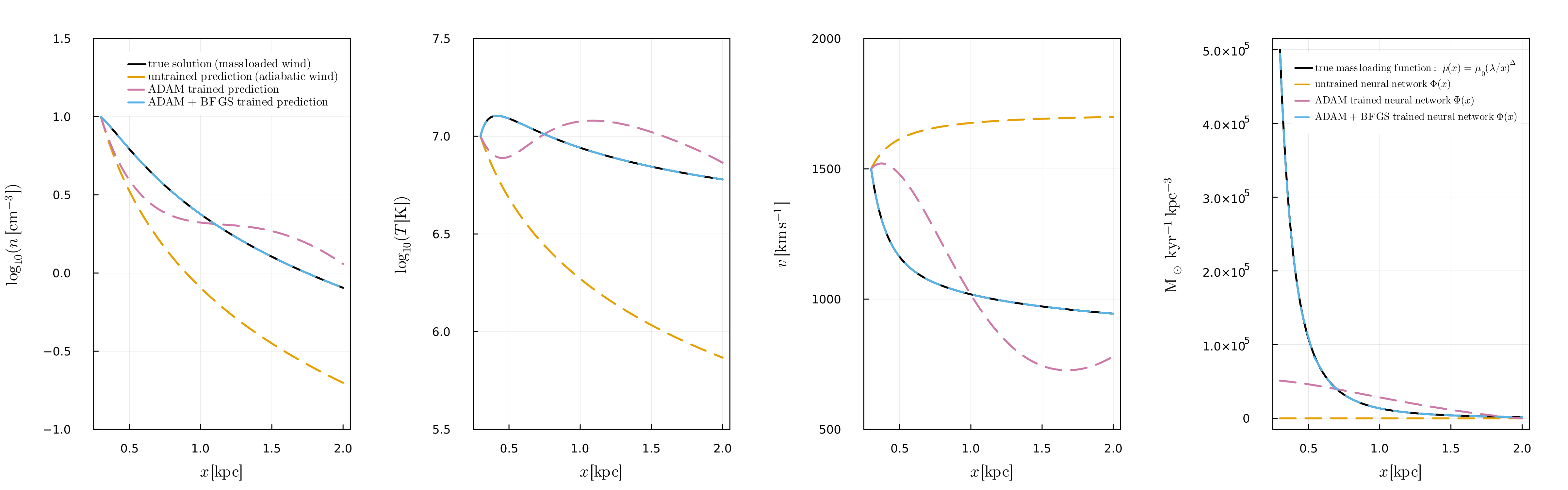
Figure 2: Density, temperature, and velocity profiles for solutions (left 3 panels) calculated with the mass-loading (right panel) given by the true function (black solid) and the output of neural networks (colored dashed). After BFGS and ADAM training, the three kinematic and thermodynamic profiles are well-matched (blue dashed on black lines), and the underlying mass-loading function was learned.

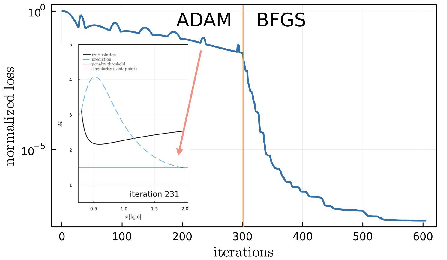
Figure 3: Learning curve for training neural network $\Phi(x)$ to learn underlying volumetric mass-loading rate $\dot{\mu}$ from the solved wind solutions. The bumps in the loss function during ADAM training epochs are attributed to penalties for near-diverging solutions.

Learning Surface Area Expansion: We now test the neural network’s ability to learn properties of the flow geometry $A(x)=A_{0}(1+(x/\eta)^{2})$, which describes a flared-cylinder flow tube that has previously been used for solar coronal hole flux tubes (Kopp & Holzer, 1976) and Milky-Way disk winds (Everett et al., 2008). Qualitatively, this function implies a roughly constant flow area up until $\eta$ when the flow begins to undergo spherical expansion. For illustration, Equation 1 can be expanded into differential form as: $d\ln\rho/dx+d\ln v/dx+d\ln A/dx=\dot{\mu}/\rho v$. This means that the effects of flow geometry are governed specifically by the surface area expansion rate $d\,\ln A/dx$, and not the magnitude of $A(x)$ (e.g., flows expanding into $4\pi x^{2}$ or $2\pi x^{2}$ behave the same). Setting $\dot{\mu}=0$ we generate the training dataset using $A(x)=A_{0}(1+(x/\eta)^{2})$ so that $d\ln A/dx=2x/(\eta^{2}+x^{2})$, where $A_{0}=0.25\,\mathrm{kpc}$ and $\eta=1.0\,$kpc. We now “forget” $d\ln A/dx$, replacing it with neural network $\Phi(x)$. Again, we initialize the neural network with output of approximately 0. This implies that the first prediction solution is identical to an adiabatic planar wind (i.e., $A(x)\simeq\mathrm{constant}$). We train for 300 iterations using ADAM with a learning rate of $0.01$ and exponential decay rate of $0.98$, followed by additional iterations using BFGS. We take $\kappa=0.1$ and $\omega=0.1$. Optimization with BFGS converges to the set gradient tolerance after 47 iterations.

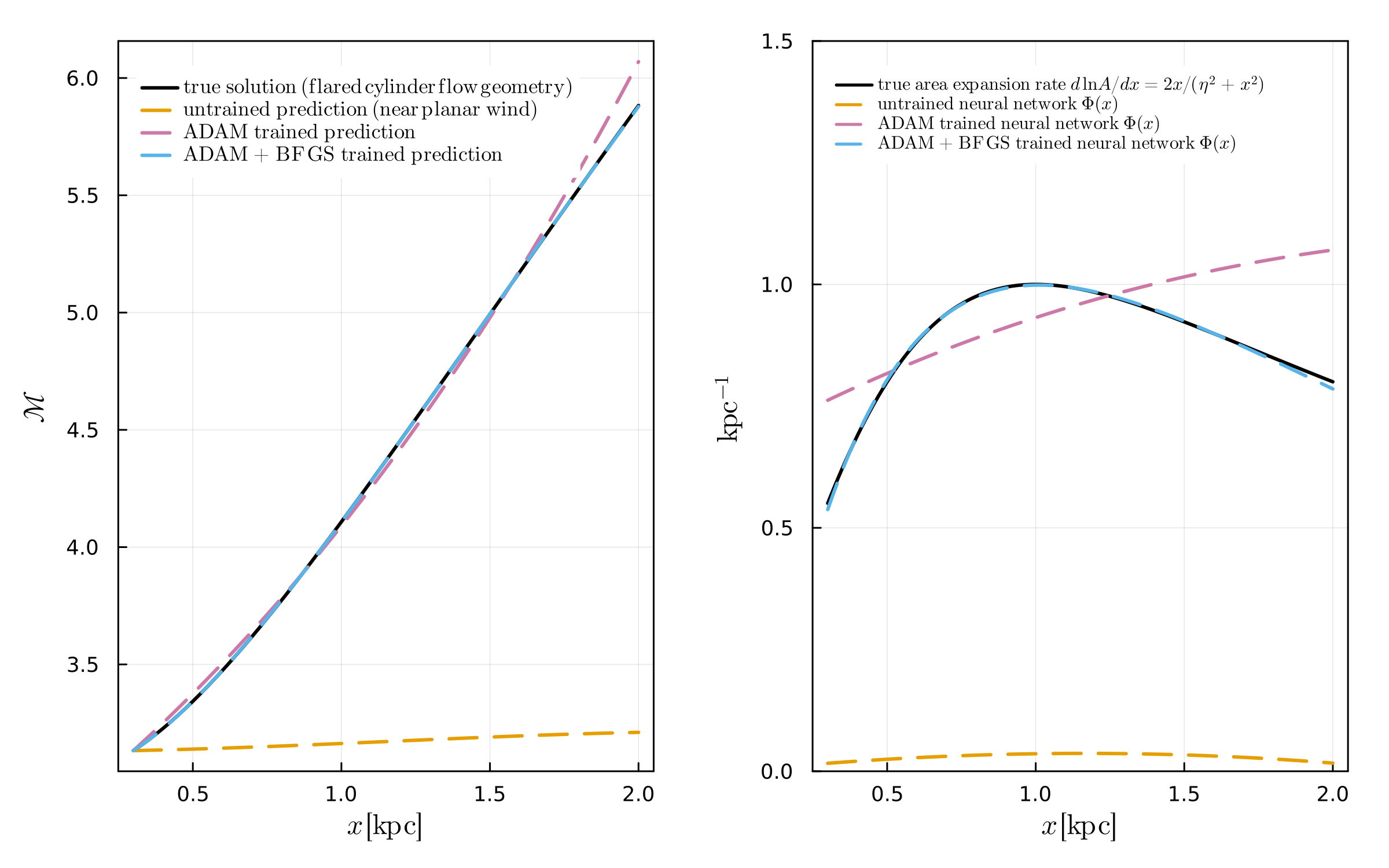
Figure 4: Left: Mach number solutions calculated with the true area function (black solid), predictions from the neural ODEs (colored dashed lines). Right: The true surface area expansion rate for a flared cylinder $d\log A/dx$ (black solid) and the output from neural network $\Phi(x)$ for various degrees of training.

In the left panel of Figure 4, we plot the Mach number solution calculated with the true area function (black line) and from predictions of the neural ODEs with varied degrees of training (colored dashed lines). We see that the best fitting line is, again, the model that underwent both ADAM and BFGS optimization. In the right panel we plot the surface area expansion rate calculated for the true surface area function (black), and the direct output of neural networks (colored dashed), finding agreement between the two (blue dashed and solid black).

4 Conclusion and Future Work

In this work we show that deep neural networks embedded as individual terms within astrophysical wind equations can discover the true functional form of both mass-loading and flow geometry expansion, without any prior knowledge. Additionally, to our knowledge at the time of writing, this is the first use of the UDE framework for coupled ODEs that contain singularities (i.e., poles at $\mathcal{M}=1$). To avoid diverging solutions, we introduced a penalty term that activates when the predicted solution falls within a threshold. This method is shown to be effective, and guides the optimization away from diverging solutions (Fig. 3). We require BFGS optimization after ADAM to converge to the functional form of the true solution. BFGS is a quasi-Newton method that uses second-order derivative information that outperforms ADAM here at low values of normalized loss. We note that using ADAM at the beginning of training is still beneficial, as it is faster and can overcome local minima better. We demonstrate the same neural network architecture can be used to learn two very different types of physics. We show that the outputs of the neural network are interpretable (Figs. 2 and 4). We find that training on the Mach number $\mathcal{M}$ outperformed training on the conserved variables $v$, $\rho$, and $P$. Beyond winds, we expect neural ODEs to be useful in discovering physics in other non-linear systems.

In future work we would like to explore the predictive power of the trained neural networks, beyond the training dataset. Here, we specifically studied the ability of a neural network embedded within coupled ODEs to accurately capture physics during supervised training, and showcase the interpretability of the result. One possible direction is to use the SINDy (Brunton et al., 2016) algorithm to extract symbolic representations of the trained neural networks which has been shown to be useful in creating hybrid models capable of making accurate long-term predictions for partially observed non-linear systems (Rackauckas et al., 2020; Santana et al., 2023; Fronk & Petzold, 2023). However, this approach requires the creation of a basis function library, which may not be generally applicable, especially when complicated non-polynomial functions are involved. If we continue to use the direct output of the trained neural network, careful considerations will need to be made towards: 1. more advanced neural network architectures that better capture long-term dependencies such as LSTMs (as opposed to the simple forward-feed neural network used here), and 2. overfitting. Additionally, future work will investigate how noisy data may affect learning outcomes. We note that even in cases where predictive power beyond the training dataset is limited, the use of neural ODEs as a discovery tool for a contained dataset is still useful, as we demonstrate here.

References

- Brunton et al. (2016) Brunton, S. L., Proctor, J. L., and Kutz, J. N. Discovering governing equations from data by sparse identification of nonlinear dynamical systems. Proceedings of the National Academy of Sciences, 113(15):3932–3937, 2016. doi: 10.1073/pnas.1517384113.
- Chen et al. (2019) Chen, R. T. Q., Rubanova, Y., Bettencourt, J., and Duvenaud, D. Neural ordinary differential equations, 2019.
- Chevalier & Clegg (1985) Chevalier, R. A. and Clegg, A. W. Wind from a starburst galaxy nucleus. Nature, 317(6032):44–45, Sep 1985. doi: 10.1038/317044a0.
- Cowie et al. (1981) Cowie, L. L., McKee, C. F., and Ostriker, J. P. Supernova remnant revolution in an inhomogeneous medium. I - Numerical models. The Astrophysical Journal, 247:908–924, Aug 1981. doi: 10.1086/159100.
- Everett et al. (2008) Everett, J. E., Zweibel, E. G., Benjamin, R. A., McCammon, D., Rocks, L., and Gallagher, III, J. S. The Milky Way’s Kiloparsec-Scale Wind: A Hybrid Cosmic-Ray and Thermally Driven Outflow. The Astrophysical Journal, 674:258–270, February 2008. doi: 10.1086/524766.
- Faucher-Giguere & Oh (2023) Faucher-Giguere, C.-A. and Oh, S. P. Key Physical Processes in the Circumgalactic Medium. arXiv e-prints, art. arXiv:2301.10253, January 2023. doi: 10.48550/arXiv.2301.10253.
- Fronk & Petzold (2023) Fronk, C. and Petzold, L. Interpretable polynomial neural ordinary differential equations. Chaos: An Interdisciplinary Journal of Nonlinear Science, 33(4):043101, 2023. doi: 10.1063/5.0130803.
- Gelbrecht et al. (2021) Gelbrecht, M., Boers, N., and Kurths, J. Neural partial differential equations for chaotic systems. New Journal of Physics, 23(4):043005, April 2021. doi: 10.1088/1367-2630/abeb90.
- Goodfellow et al. (2016) Goodfellow, I., Bengio, Y., and Courville, A. Deep Learning. The MIT Press, Cambridge, MA, 2016. ISBN 9780262035613.
- Gronke & Oh (2018) Gronke, M. and Oh, S. P. The growth and entrainment of cold gas in a hot wind. Monthly Notices of the Royal Astronomical Society, 480(1):L111–L115, October 2018. doi: 10.1093/mnrasl/sly131.
- Gronke & Oh (2020) Gronke, M. and Oh, S. P. How cold gas continuously entrains mass and momentum from a hot wind. Monthly Notices of the Royal Astronomical Society, 492(2):1970–1990, February 2020. doi: 10.1093/mnras/stz3332.
- Hornik et al. (1990) Hornik, K., Stinchcombe, M., and White, H. Universal approximation of an unknown mapping and its derivatives using multilayer feedforward networks. Neural Networks, 3(5):551–560, 1990. ISSN 0893-6080. doi: https://doi.org/10.1016/0893-6080(90)90005-6. URL https://www.sciencedirect.com/science/article/pii/0893608090900056.
- Keith et al. (2021) Keith, B., Khadse, A., and Field, S. E. Learning orbital dynamics of binary black hole systems from gravitational wave measurements. Physical Review Research, 3(4):043101, November 2021. doi: 10.1103/PhysRevResearch.3.043101.
- Kim et al. (2020) Kim, C.-G., Ostriker, E. C., Fielding, D. B., Smith, M. C., Bryan, G. L., Somerville, R. S., Forbes, J. C., Genel, S., and Hernquist, L. A Framework for Multiphase Galactic Wind Launching Using TIGRESS. The Astrophysical Journal Letters, 903(2):L34, November 2020. doi: 10.3847/2041-8213/abc252.
- Klein et al. (1994) Klein, R. I., McKee, C. F., and Colella, P. On the Hydrodynamic Interaction of Shock Waves with Interstellar Clouds. I. Nonradiative Shocks in Small Clouds. The Astrophysical Journal, 420:213, January 1994. doi: 10.1086/173554.
- Kopp & Holzer (1976) Kopp, R. A. and Holzer, T. E. Dynamics of coronal hole regions. I. Steady polytropic flows with multiple critical points. solphys, 49(1):43–56, July 1976. doi: 10.1007/BF00221484.
- Kuwahara & Bauch (2023) Kuwahara, B. S. and Bauch, C. T. Predicting covid-19 pandemic waves with biologically and behaviorally informed universal differential equations. In medRxiv, 2023.
- Lamers & Cassinelli (1999) Lamers, H. J. G. L. M. and Cassinelli, J. P. Introduction to Stellar Winds. 1999.
- LeCun et al. (2015) LeCun, Y., Bengio, Y., and Hinton, G. Deep Learning. Nature, New York, NY, 2015. doi: 10.1038/nature14539. URL https://www.nature.com/articles/nature14539.
- Lopez et al. (2020) Lopez, L. A., Mathur, S., Nguyen, D. D., Thompson, T. A., and Olivier, G. M. Temperature and Metallicity Gradients in the Hot Gas Outflows of M82. The Astrophysical Journal, 904(2):152, December 2020. doi: 10.3847/1538-4357/abc010.
- Lu et al. (2021) Lu, Q., Mao, Z., Zuo, W., and Dong, B. Learning nonlinear operators via deeponet based on the universal approximation theorem of operators. Nature Machine Intelligence, 3:270–278, 2021. doi: 10.1038/s42256-021-00302-5. URL https://www.nature.com/articles/s42256-021-00302-5.
- Meiss (2007) Meiss, J. D. Differential Dynamical Systems. Society for Industrial and Applied Mathematics, 2007. doi: 10.1137/1.9780898718232. URL https://epubs.siam.org/doi/abs/10.1137/1.9780898718232.
- Nguyen & Thompson (2021) Nguyen, D. D. and Thompson, T. A. Mass-loading and non-spherical divergence in hot galactic winds: implications for X-ray observations. Monthly Notices of the Royal Astronomical Society, October 2021. doi: 10.1093/mnras/stab2910.
- Nguyen et al. (2023) Nguyen, D. D., Thompson, T. A., Schneider, E. E., Lopez, S., and Lopez, L. A. Dynamics of hot galactic winds launched from spherically-stratified starburst cores. Monthly Notices of the Royal Astronomical Society, 518(1):L87–L91, January 2023. doi: 10.1093/mnrasl/slac141.
- Pandya et al. (2022) Pandya, V., Fielding, D. B., Bryan, G. L., Carr, C., Somerville, R. S., Stern, J., Faucher-Giguere, C.-A., Hafen, Z., and Angles-Alcazar, D. A unified model for the co-evolution of galaxies and their circumgalactic medium: the relative roles of turbulence and atomic cooling physics. arXiv e-prints, art. arXiv:2211.09755, November 2022. doi: 10.48550/arXiv.2211.09755.
- Quataert et al. (2022a) Quataert, E., Jiang, Y.-F., and Thompson, T. A. The physics of galactic winds driven by cosmic rays - II. Isothermal streaming solutions. Monthly Notices of the Royal Astronomical Society, 510(1):920–945, February 2022a. doi: 10.1093/mnras/stab3274.
- Quataert et al. (2022b) Quataert, E., Thompson, T. A., and Jiang, Y.-F. The physics of galactic winds driven by cosmic rays I: Diffusion. Monthly Notices of the Royal Astronomical Society, 510(1):1184–1203, February 2022b. doi: 10.1093/mnras/stab3273.
- Rackauckas & Nie (2017) Rackauckas, C. and Nie, Q. Differentialequations.jl–a performant and feature-rich ecosystem for solving differential equations in julia. Journal of Open Research Software, 5(1):15, 2017.
- Rackauckas et al. (2020) Rackauckas, C., Ma, Y., Martensen, J., Warner, C., Zubov, K., Supekar, R., Skinner, D., and Ramadhan, A. Universal differential equations for scientific machine learning. arXiv preprint arXiv:2001.04385, 2020.
- Revels et al. (2016) Revels, J., Lubin, M., and Papamarkou, T. Forward-mode automatic differentiation in Julia. arXiv:1607.07892 [cs.MS], 2016. URL https://arxiv.org/abs/1607.07892.
- Santana et al. (2023) Santana, V. V., Costa, E., Rebello, C. M., Mafalda Ribeiro, A., Rackauckas, C., and Nogueira, I. B. R. Efficient hybrid modeling and sorption model discovery for non-linear advection-diffusion-sorption systems: A systematic scientific machine learning approach. arXiv e-prints, art. arXiv:2303.13555, March 2023. doi: 10.48550/arXiv.2303.13555.
- Schneider & Robertson (2015) Schneider, E. E. and Robertson, B. E. CHOLLA: A New Massively Parallel Hydrodynamics Code for Astrophysical Simulation. The Astrophysical Journal Supplement Series, 217(2):24, April 2015. doi: 10.1088/0067-0049/217/2/24.
- Smith et al. (2023) Smith, M. C., Fielding, D. B., Bryan, G. L., Kim, C.-G., Ostriker, E. C., Somerville, R. S., Stern, J., Su, K.-Y., Weinberger, R., Hu, C.-Y., Forbes, J. C., Hernquist, L., Burkhart, B., and Li, Y. Arkenstone I: A Novel Method for Robustly Capturing High Specific Energy Outflows In Cosmological Simulations. arXiv e-prints, art. arXiv:2301.07116, January 2023. doi: 10.48550/arXiv.2301.07116.
- Stepaniants et al. (2023) Stepaniants, G., Hastewell, A. D., Skinner, D. J., Totz, J. F., and Dunkel, J. Discovering dynamics and parameters of nonlinear oscillatory and chaotic systems from partial observations. arXiv e-prints, art. arXiv:2304.04818, April 2023. doi: 10.48550/arXiv.2304.04818.
- Strickland & Heckman (2009) Strickland, D. K. and Heckman, T. M. Supernova Feedback Efficiency and Mass Loading in the Starburst and Galactic Superwind Exemplar M82. The Astrophysical Journal, 697:2030–2056, June 2009. doi: 10.1088/0004-637X/697/2/2030.
- Tan & Fielding (2023) Tan, B. and Fielding, D. B. Cloud Atlas: Navigating the Multiphase Landscape of Tempestuous Galactic Winds. arXiv e-prints, art. arXiv:2305.14424, May 2023. doi: 10.48550/arXiv.2305.14424.
- Tsitouras (2011) Tsitouras, C. Runge–kutta pairs of order 5(4) satisfying only the first column simplifying assumption. Computers & Mathematics with Applications, 62(2):770–775, 2011. ISSN 0898-1221. doi: https://doi.org/10.1016/j.camwa.2011.06.002. URL https://www.sciencedirect.com/science/article/pii/S0898122111004706.
- Vortmeyer-Kley et al. (2021) Vortmeyer-Kley, R., Nieters, P., and Pipa, G. A trajectory-based loss function to learn missing terms in bifurcating dynamical systems. Scientific Reports, 11:21181, Oct 2021. doi: 10.1038/s41598-021-99609-x. URL https://www.nature.com/articles/s41598-021-99609-x.
- Wibking & Krumholz (2022) Wibking, B. D. and Krumholz, M. R. QUOKKA: a code for two-moment AMR radiation hydrodynamics on GPUs. Monthly Notices of the Royal Astronomical Society, 512(1):1430–1449, May 2022. doi: 10.1093/mnras/stac439.
- Wigner (1960) Wigner, E. P. The unreasonable effectiveness of mathematics in the natural sciences. Communications on Pure and Applied Mathematics, 13(1):1–14, 1960.
- Yin et al. (2023) Yin, S., Wu, J., and Song, P. Optimal control by deep learning techniques and its applications on epidemic models. Journal of Mathematical Biology, 87:2121–2148, Apr 2023. doi: 10.1007/s00285-023-01873-0. URL https://link.springer.com/article/10.1007/s00285-023-01873-0.
- Yuan et al. (2023) Yuan, Y., Krumholz, M. R., and Martin, C. L. The observable properties of cool winds from galaxies, AGN, and star clusters - II. 3D models for the multiphase wind of M82. Monthly Notices of the Royal Astronomical Society, 518(3):4084–4105, January 2023. doi: 10.1093/mnras/stac3241.