Symplectic lattice gauge theories in the grid framework: Approaching the conformal window

Abstract

Symplectic gauge theories coupled to matter fields lead to symmetry enhancement phenomena that have potential applications in such diverse contexts as composite Higgs, top partial compositeness, strongly interacting dark matter, and dilaton-Higgs models. These theories are also interesting on theoretical grounds, for example in reference to the approach to the large-$N$ limit. A particularly compelling research aim is the determination of the extent of the conformal window in gauge theories with symplectic groups coupled to matter, for different groups and for field content consisting of fermions transforming in different representations. Such determination would have far-reaching implications, but requires overcoming huge technical challenges.

Numerical studies based on lattice field theory can provide the quantitative information necessary to this endeavour. We developed new software to implement symplectic groups in the Monte Carlo algorithms within the Grid framework. In this paper, we focus most of our attention on the $Sp(4)$ lattice gauge theory coupled to four (Wilson-Dirac) fermions transforming in the 2-index antisymmetric representation, as a case study. We discuss an extensive catalogue of technical tests of the algorithms and present preliminary measurements to set the stage for future large-scale numerical investigations. We also include the scan of parameter space of all asymptotically free $Sp(4)$ lattice gauge theories coupled to varying number of fermions transforming in the antisymmetric representation.

I Introduction

Gauge theories with symplectic group, $Sp(2N)$, in four space-time dimensions have been proposed as the microscopic origin of several new physics models that stand out in the literature for their simplicity and elegance. We list some compelling examples later in this introduction. Accordingly, lattice field theory methods have been deployed to obtain numerically a first quantitative characterisation of the strongly coupled dynamics of such gauge theories Bennett:2017kga ; Lee:2018ztv ; Bennett:2019jzz ; Bennett:2019cxd ; Bennett:2020hqd ; Bennett:2020qtj ; Lucini:2021xke ; Bennett:2021mbw ; Bennett:2022yfa ; Bennett:2022gdz ; Bennett:2022ftz ; AS ; Lee:2022elf ; Hsiao:2022kxf ; Bennett:2023rsl ; Maas:2021gbf ; Zierler:2021cfa ; Kulkarni:2022bvh ; Bennett:2023wjw . Different regions of lattice parameter space have been explored; by varying the rank of the group, $N$, the number, $N_{\rm f,as}$, and mass, $m^{\rm f,as}$, of (Dirac) fermions transforming in the fundamental (${\rm f}$) and 2-index antisymmetric (${\rm as}$) representation, one can tabulate the properties of these theories. And, after taking infinite volume and continuum limits, the results can be used by model builders, phenomenologists, and field theorists working on potential applications.

A prominent role in the recent literature is played by the theory with $N=2$, $N_{\rm f}=2$, and $N_{\rm as}=3$. It gives rise, at low energies, to the effective field theory (EFT) entering the minimal Composite Higgs model (CHM) that is amenable to lattice studies Barnard:2013zea , and also realises top (partial) compositeness Kaplan:1991dc (see also Refs. Grossman:1999ra ; Gherghetta:2000qt ). It hence provides an economical way of explaining the microscopic origin of the two heaviest particles in the standard model, the Higgs boson and the top quark, singling them out as portals to new physics.

The $Sp(2N)$ gauge theories with $N_{\rm f}=2$ and $N_{\rm as}=0$ find application also in the simplest realisations of the strongly interacting massive particle (SIMP) scenario for dark matter Hochberg:2014dra ; Hochberg:2014kqa ; Hochberg:2015vrg ; Bernal:2017mqb ; Berlin:2018tvf ; Bernal:2019uqr ; Tsai:2020vpi ; Kondo:2022lgg ; Bernal:2015xba . They can address observational puzzles such as the ‘core vs. cusp’ deBlok:2009sp and ‘too big to fail’ Boylan-Kolchin:2011qkt problems. In addition, they might have profound implications in the physics of the early universe and be testable in present and future gravitational wave experiments Seto:2001qf ; Kawamura:2006up ; Crowder:2005nr ; Corbin:2005ny ; Harry:2006fi ; Hild:2010id ; Yagi:2011wg ; Sathyaprakash:2012jk ; Thrane:2013oya ; Caprini:2015zlo ; LISA:2017pwj ; LIGOScientific:2016wof ; Isoyama:2018rjb ; Baker:2019nia ; Brdar:2018num ; Reitze:2019iox ; Caprini:2019egz ; Maggiore:2019uih . This is because they can give rise to a relic stochastic background of gravitational waves Witten:1984rs ; Kamionkowski:1993fg ; Allen:1996vm ; Schwaller:2015tja ; Croon:2018erz ; Christensen:2018iqi , that are the current subject of active study Huang:2020crf ; Halverson:2020xpg ; Kang:2021epo .

On a more abstract, theoretical side, in $Sp(2N)$ Yang-Mills theories one can compute numerically the spectra of glueballs and strings Lucini:2001ej ; Lucini:2004my ; Lucini:2010nv ; Lucini:2012gg ; Athenodorou:2015nba ; Lau:2017aom ; Hernandez:2020tbc ; Athenodorou:2021qvs ; Yamanaka:2021xqh ; Bonanno:2022yjr , as well as the topological charge and susceptibility Luscher:1981zq ; Campostrini:1989dh ; DelDebbio:2002xa ; Lucini:2004yh ; DelDebbio:2004ns ; Luscher:2010ik ; Panagopoulos:2011rb ; Bonati:2015sqt ; Bonati:2016tvi ; Ce:2016awn ; Alexandrou:2017hqw ; Bonanno:2020hht ; Borsanyi:2021gqg ; Cossu:2021bgn ; Teper:2022mmj ; Bonanno:2022vot ; Bonanno:2022hmz . This allows for a comparison with other gauge groups ($SU(N_{c})$ in particular), by means of which to test non-perturbative ideas about field theories and their approach to the large-$N_{c}$ limit—see, e.g., Refs. Bochicchio:2016toi ; Bochicchio:2013sra ; Hong:2017suj ; Bennett:2020hqd ; Bennett:2022gdz . Indeed, even the pioneering lattice study of symplectic theories in Ref. Holland:2003kg was performed to the purpose of better characterising on general grounds the deconfinement phase transition.

A special open problem is that of the highly non-trivial determination of the extent of the conformal window in strongly coupled gauge theories with matter field content. It has both theoretical and phenomenological implications, of general interest to model-builders, phenomenologists, and field theorists alike. Particular attention has been so far paid to $SU(N_{c})$ theories, more than $Sp(2N)$ (with $N>1$) ones. Let us pause and explain what the problem is, on general grounds. Robust perturbation-theory arguments show that if the number of matter fields is large enough—but not so much as to spoil asymptotic freedom—gauge theories can be realised in a conformal phase. This is the case when long distance physics is governed by a fixed point of the renormalisation group (RG) evolution Caswell:1974gg ; Banks:1981nn , and the fixed point is described by a conformal field theory (CFT). It is reasonable to believe that such fixed points may exist also outside the regime of validity of perturbation theory, when the number of matter fields is smaller. What is the smallest number of fermions for which the theory still admits a fixed point, rather than confining in the infrared (IR), is an open question. While gaining some control over non-perturbative physics is possible in supersymmetric theories (see Ref. Intriligator:1995au and references therein), the non-supersymmetric ones are the subject of a rich and fascinating literature Appelquist:1988yc ; Cohen:1988sq ; Sannino:2004qp ; Dietrich:2006cm ; Ryttov:2007cx ; Pica:2010mt ; Pica:2010xq ; Kim:2020yvr ; Lee:2020ihn , part of which uses perturbative instruments and high-loop expansions Baikov:2016tgj ; Herzog:2017ohr ; Ryttov:2016ner ; Ryttov:2016hdp ; Ryttov:2016asb ; Ryttov:2016hal ; Ryttov:2017toz ; Ryttov:2017kmx ; Ryttov:2017dhd ; Gracey:2018oym ; Ryttov:2018uue ; Ryttov:2020scx ; Ryttov:2023uzc , but there is no firm agreement on the results—we include a brief overview of work in this direction, in the body of the paper.

Knowledge of the extent of the conformal window also has relevant phenomenological implications. Various arguments suggest that at the lower edge of the conformal window, the anomalous dimensions of the CFT operators might be so large as to invalidate naive dimensional analysis (NDA) expectations for the scaling of observable quantities Cohen:1988sq ; Kaplan:2009kr . And it has been speculated that this might affect even confining theories that live outside the conformal window, with applications to technicolor, CHMs, top (partial) compositeness, SIMP dark matter (e.g., see Refs. Panico:2015jxa ; Witzel:2019jbe ; Cacciapaglia:2020kgq ; Chivukula:2000mb ; Lane:2002wv ; Hill:2002ap ; Martin:2008cd ; Sannino:2009za ; Piai:2010ma and references therein).

Lattice studies of the extent of the conformal window have mostly focused on $SU(N_{c})$ groups, with fermion matter in various representations of the gauge group. Closely related to these studies is the emergence, in $SU(3)$ gauge theories with eight (Dirac) fermions transforming in the fundamental representation LatKMI:2014xoh ; Appelquist:2016viq ; LatKMI:2016xxi ; Gasbarro:2017fmi ; LatticeStrongDynamics:2018hun ; LatticeStrongDynamicsLSD:2021gmp ; Hasenfratz:2022qan ; LSD:2023uzj ; LatticeStrongDynamics:2023bqp , or (Dirac) fermions transforming in the 2-index symmetric representation Fodor:2012ty ; Fodor:2015vwa ; Fodor:2016pls ; Fodor:2017nlp ; Fodor:2019vmw ; Fodor:2020niv , of numerical evidence pointing to the existence of a light isosinglet scalar state, that is tempting to identify with the dilaton, the PNGB associated with dilatations.

It has been predicted long ago that a light dilaton should exist in strongly coupled, confining theories living in proximity of the lower end of the conformal window Leung:1985sn ; Bardeen:1985sm ; Yamawaki:1985zg , and the EFT description of such state has a remote historical origin Migdal:1982jp ; Coleman:1985rnk . It might have huge consequences in extensions of the standard model Goldberger:2008zz . A plethora of phenomenological studies exists on the dilaton (see, for example, Refs. Hong:2004td ; Dietrich:2005jn ; Hashimoto:2010nw ; Appelquist:2010gy ; Vecchi:2010gj ; Chacko:2012sy ; Bellazzini:2012vz ; Bellazzini:2013fga ; Abe:2012eu ; Eichten:2012qb ; Hernandez-Leon:2017kea ; CruzRojas:2023jhw and references therein). The $SU(3)$ lattice evidence for the existence of this state has triggered renewed interest in the dilaton effective field theory (dEFT), which combines the chiral Lagrangian description of the PNGBs associated with the internal global symmetries of the system, with the additional, light scalar, interpreted as a dilaton Matsuzaki:2013eva ; Golterman:2016lsd ; Kasai:2016ifi ; Hansen:2016fri ; Golterman:2016cdd ; Appelquist:2017wcg ; Appelquist:2017vyy ; Golterman:2018mfm ; Cata:2019edh ; Cata:2018wzl ; Appelquist:2019lgk ; Golterman:2020tdq ; Golterman:2020utm ; Appelquist:2020bqj ; Appelquist:2022qgl ; Appelquist:2022mjb .

The aforementioned lattice studies of symplectic theories, motivated by CHMs and SIMPs, can be carried out with comparatively modest resources, and using lattices of modest sizes, because they require exploring the intermediate mass range for the mesons in the theory. By contrast, the study of the deep-IR properties of $Sp(2N)$ gauge theories requires investigating the low mass regime of the fermions, for which one needs lattices and ensembles big enough to overcome potentially large finite size effects and long autocorrelation times. The supercomputing demands (both on hardware and software) of these calculations are such that a new dedicated set of instruments, and a long-term research strategy, is needed to make these investigations feasible. With this paper, we make the first, propaedeutic, technical steps on the path towards determining on the lattice the extent of the conformal window in theories with $Sp(2N)$ group, for $N>1$.

To this end, we elected to build, test, and make publicly available new software githubsp2n , that supplements previous releases of the Grid library Boyle:2015tjk ; Boyle:2016lbp ; Yamaguchi:2022feu ; github , by adding to it new functionality specifically designed to handle $Sp(2N)$ theories with matter fields in multiple representations. The resulting software takes advantage of all the features offered by the modularity and flexibility of Grid, in particular its ability to work both on CPU- as well as GPU-based architectures. We present two types of preliminary results relevant to this broader endeavour: technical tests of the algorithm and of the physics outcomes are supplemented by preliminary analyses, conducted on coarse lattices, of the parameter space of the lattice theory. The latter set the stage for future large-scale numerical studies, by identifying the regions of parameter space connected to continuum physics. The former are intended to validate the software, and test its performance for symplectic theories on machines with GPU architecture. Unless otherwise specified, we use the $Sp(4)$ theory, coupled to $N_{\rm as}=4$ Wilson-Dirac fermions transforming in the 2-index antisymmetric representation, as a case study. The lessons we learn from the results we report have general validity and applicability.

This paper is organised as follows. We start by defining the $Sp(2N)$ gauge theories of interest in Sect. II, both in the continuum and on the lattice. We also summarise briefly the current understanding of the extent of the conformal window in these theories. Section III discusses the software implementation of $Sp(2N)$ on Grid, and the basic tests we performed on the algorithm. In Sect. IV we concentrate on lattice theories in which the fermions do not contribute to the dynamics, focusing both on the Yang-Mills theory and the quenched approximation. New results about the bulk structure of all the $Sp(4)$ theories coupled to (Wilson-Dirac) fermions transforming in the 2-index antisymmetric representation can be found in Sect. V, while Sect. VI discusses scale setting (Wilson flow) and topology. A brief summary and outlook concludes the paper, in Sect. VII. Additional technical details are relegated to the appendix.

II Gauge theories with symplectic group

The $Sp(2N)$ continuum field theories of interest (with $N>1$), written in Minkowski space with signature mostly ‘$-$’, have the following Lagrangian density (we borrow notation and conventions from Ref. Bennett:2019cxd ):

$${\cal L} = -\frac{1}{2}{\rm Tr}\ G_{\mu\nu}G^{\mu\nu}\,+\,\frac{1}{2}\sum_{i}^{N_{\rm f}}\left(i\overline{Q^{i}}_{a}\gamma^{\mu}\left(D_{\mu}Q^{i}\right)^{a}\,-\,i\overline{D_{\mu}Q^{i}}_{a}\gamma^{\mu}Q^{i\,a}\right)\,-\,m^{\rm f}\sum_{i}^{N_{\rm f}}\overline{Q^{i}}_{a}Q^{i\,a}+$$ (1)

$$\,+\,\frac{1}{2}\sum_{k}^{N_{\rm as}}\left(i\overline{\Psi^{k}}_{ab}\gamma^{\mu}\left(D_{\mu}\Psi^{k}\right)^{ab}\,-\,i\overline{D_{\mu}\Psi^{k}}_{ab}\gamma^{\mu}\Psi^{k\,ab}\right)\,-\,m^{\rm as}\sum_{k}^{N_{\rm as}}\overline{\Psi^{k}}_{ab}\Psi^{k\,ab}\,.$$

The fields $Q^{i\,a}$, with $i=1,\,\cdots,\,N_{\rm f}$, are Dirac fermions that transform in the fundamental representation of $Sp(2N)$, as indicated by the index $a=1,\,\cdots,\,2N$, while the $\Psi^{k\,ab}$ ones, with $k=1,\,\cdots,\,N_{\rm as}$, transform in the 2-index antisymmetric representation of the gauge group. The covariant derivatives are defined by making use of the transformation properties under the action of an element $U$ of the $Sp(2N)$ gauge group, according to which

$$Q\rightarrow UQ\,,~{}~{}~{}{\rm and}~{}~{}~{}\Psi\rightarrow U\Psi U^{\mathrm{T}}\,.$$ (2)

They can be written in terms of the gauge field $A_{\mu}\equiv A_{\mu}^{a}t^{a}$, where $t^{a}$ are the generators of $Sp(2N)$, normalised so that ${\rm Tr}\ t^{a}t^{b}=\frac{1}{2}\delta^{ab}$, to read as follows:

$$D_{\mu}Q^{i} = \partial_{\mu}Q^{i}\,+\,igA_{\mu}Q^{i}\,,$$ (3)

$$D_{\mu}\Psi^{j} = \partial_{\mu}\Psi^{j}\,+\,igA_{\mu}\Psi^{j}\,+\,ig\Psi^{j}A_{\mu}^{\mathrm{T}}\,,$$ (4)

where $g$ is the gauge coupling. The field-strength tensor is given by

$$G_{\mu\nu} \equiv \partial_{\mu}A_{\nu}-\partial_{\nu}A_{\mu}+ig\left[A_{\mu}\,,\,A_{\nu}\right]\,,$$ (5)

where $[\cdot\,,\cdot]$ is the commutator.

The form of Eq. (1) makes it easy to show that the $SU(N_{\rm f})_{L}\times SU(N_{\rm f})_{R}$ and $SU(N_{\rm as})_{L}\times SU(N_{\rm as})_{R}$ global symmetries acting on the flavor indexes of $Q^{i}$ and $\Psi^{k}$, respectively, are enhanced to $SU(2N_{\rm f})$ and $SU(2N_{\rm as})$. By rewriting Eq. (1) in terms of 2-component fermions Lewis:2011zb ; Bennett:2019cxd ,

$$Q^{i\,a}=\begin{pmatrix}q^{i\,a}\\ \Omega^{ab}\left(-\tilde{C}q^{i+2,*}\right)_{b}\end{pmatrix}\,,\;\Psi^{k\,ab}=\begin{pmatrix}\psi^{k\,ab}\\ \Omega^{ab}\Omega^{bd}\left(-\tilde{C}q^{k+3,*}\right)_{cd}\end{pmatrix}\,,$$ (6)

($\tilde{C}=-i\tau^{2}$, $\tau^{2}$ is the second Pauli matrix) we get the Lagrangian where the global symmetries are manifest

$${\cal L} = -\frac{1}{2}{\rm Tr}\ G_{\mu\nu}G^{\mu\nu}\,+\,\frac{1}{2}\sum_{j}^{2N_{\rm f}}\left(i\left(q^{j}\right)^{\dagger}_{a}\bar{\sigma}^{\mu}\left(D_{\mu}q^{j}\right)^{a}-i\left(D_{\mu}q^{j}\right)^{\dagger}_{a}\bar{\sigma}^{\mu}\left(q^{j}\right)^{a}\right)+$$ (7)

$$\,-\,\dfrac{1}{2}m^{\rm f}\sum_{j,\,k}^{2N_{\rm f}}\Omega_{jk}\left(q^{j\,a\,T}\Omega_{ab}\tilde{C}q^{k\,b}-\left(q^{j}\right)^{\dagger}_{a}\Omega^{ab}\tilde{C}\left(q^{k\,*}\right)_{b}\right)+$$

$$\,+\,\dfrac{1}{2}\sum_{k}^{2N_{\rm as}}\left(i\left(\psi^{k}\right)^{\dagger}_{ab}\bar{\sigma}^{\mu}\left(D_{\mu}\psi^{k}\right)^{ab}-i\left(D_{\mu}\psi^{k}\right)^{\dagger}_{ab}\bar{\sigma}^{\mu}\left(\psi^{k}\right)^{ab}\right)+$$

$$\,-\ \dfrac{1}{2}m^{\rm as}\sum_{j,\,k}^{2N_{\rm as}}\omega_{jk}\left(\psi^{j\,ab\,T}\Omega_{ac}\Omega_{bd}\tilde{C}\psi^{k\,cd}-\left(\psi^{j}\right)^{\dagger}_{ab}\Omega^{ac}\Omega^{bd}\tilde{C}\left(\psi^{k\,*}\right)_{cd}\right)\,,$$

where we defined $\bar{\sigma}^{\mu}\equiv\left(\mathbb{1}_{2\times 2},\tau^{i}\right)$ and $\omega_{jk}=\omega^{jk}\equiv\begin{pmatrix}\begin{matrix}\mathbb{0}\end{matrix}&\mathbb{1}_{N_{\rm as}}\\ \mathbb{1}_{N_{\rm as}}&\begin{matrix}\mathbb{0}\end{matrix}\end{pmatrix}$. The antisymmetric matrix $\Omega$ has the same form, as defined in Eq. (43) of Appendix A, for both the gauge and fundamental flavour symmetries, but the indices run with $a=1,\cdots,2N$ for the former and with $j=1,\cdots,2N_{\rm f}$ for the latter.

The mass terms break the symmetries to the maximal $Sp(2N_{\rm f})$ and $SO(2N_{\rm as})$ subgroups. Bilinear fermion condensates arise non-perturbatively, breaking the symmetries according to the same pattern, and hence one expects the presence of $N_{\rm f}(2N_{\rm f}-1)-1$ PNGBs in the $(\rm f)$ sector (for $N_{f}>1$), and $N_{\rm as}(2N_{\rm as}+1)-1$ in the $(\rm as)$ sector.

The main parameters governing the system are hence $N$, $N_{\rm f}$, and $N_{\rm as}$, and in most of the paper we refer to the theory with $N=2$, $N_{\rm f}=0$, and $N_{\rm as}=4$ as a case study. The running coupling, $g$, obeys a renormalisation group equation (RGE) in which the beta function at the 1-loop order is scheme-independent,

$$\beta = -\frac{g^{3}}{(4\pi)^{2}}b_{1},$$ (8)

and is governed by the coefficient $b_{1}$, which for a non-Abelian theory coupled to Dirac fermions can be written as

$$b_{1}=\frac{11}{3}C_{2}(G)-\frac{4}{3}N_{\rm f}\frac{d_{\rm f}}{d_{G}}C_{2}({\rm f})-\frac{4}{3}N_{\rm as}\frac{d_{\rm as}}{d_{G}}C_{2}({\rm as})\,\\$$ (9)

and, specifically for $Sp(2N)$ groups, becomes

$$b_{1}=\frac{11}{3}(N+1)-\frac{2}{3}N_{\rm f}-\frac{4}{3}N_{\rm as}\frac{N(2N-1)-1}{N(2N+1)}N\,.$$ (10)

The coefficients $C_{2}(G)$, $C_{2}(\rm{f})$, $C_{2}(\rm{as})$ are quadratic Casimir operators in the adjoint, fundamental and antisymmetric representations, while $d_{G}$, $d_{\rm f}$, $d_{\rm as}$ are the dimensions of these representations, respectively. We restrict attention to asymptotically free theories, for which $b_{1}$ is positive. For $Sp(2N)$ theories with $N_{\rm f}=0$, this requirement sets the upper bound $N_{\rm as}<\frac{11(N+1)}{4(N-1)}$, which for $N=2$ yields $N_{\rm as}<33/4$—perturbatively, ${\rm as}$-type fermions make double the contribution of ${\rm f}$-type ones, in $Sp(4)$. The spectrum of mesons depends on the mass, $m^{\rm f,as}$, of the fermions, by varying which we can test which of the following three possible classes the theory falls into.

1. The theory confines, similarly to Yang-Mills theories. One expects to find a gapped spectrum, and a set of PNGBs that become parametrically light in respect to other states, when $m^{\rm f,as}\rightarrow 0$. The small mass and momentum regime is described by chiral perturbation theory ($\chi$PT) Coleman:1969sm ; Weinberg:1978kz ; Gasser:1984gg ; Leutwyler:1993iq .

2. The theory is IR conformal. In this case, a gap arises only because of the presence of the mass terms, and would disappear into a continuum for $m^{\rm f,as}\rightarrow 0$. The spectrum and spectral density exhibit scaling, in the form described for example in Refs. Luty:2008vs ; DelDebbio:2009fd ; DeGrand:2009hu ; DelDebbio:2010hu ; DelDebbio:2010ze ; DelDebbio:2010jy ; Patella:2012da —see also Ref. Hasenfratz:2023sqa .

3. The theory is confining, but has near-conformal dynamics. As in the confining case, when $m^{\rm f,as}\rightarrow 0$ one finds massless PNGBs. An additional isosinglet scalar state, the dilaton, is also light, compared to the other mesons, and long distance physics is described by dEFT Matsuzaki:2013eva ; Golterman:2016lsd ; Kasai:2016ifi ; Hansen:2016fri ; Golterman:2016cdd ; Appelquist:2017wcg ; Appelquist:2017vyy ; Golterman:2018mfm ; Cata:2019edh ; Cata:2018wzl ; Appelquist:2019lgk ; Golterman:2020tdq ; Golterman:2020utm ; Appelquist:2020bqj ; Appelquist:2022qgl ; Appelquist:2022mjb —see also the discussions in Refs. Crewther:2020tgd ; DelDebbio:2021xwu ; Zwicky:2023bzk , and references therein.

II.1 The conformal window

The three possible classes of gauge theories described above are determined by whether the theory is, respectively, far outside, inside or just outside the boundary of the conformal window. The determination of the conformal window is tantamount to showing the existence of the IR fixed point at non-zero coupling so that the theory is interacting and IR conformal. We provide here some more detail and information about this challenging endeavour and what is known to date, starting from perturbative arguments. The coefficient of the (scheme-independent) $2$-loop RG beta function, $b_{2}$, which is found to be, for generic non-abelian gauge theories,

$$b_{2}=\frac{34}{3}C_{2}(G)^{2}-\frac{4}{3}\left(5C_{2}(G)+3C_{2}(\rm{f})\right)\frac{d_{\rm f}}{d_{G}}C_{2}(\rm{f})N_{\rm{f}}-\frac{4}{3}\left(5C_{2}(G)+3C_{2}(\rm{as})\right)\frac{d_{\rm as}}{d_{G}}C_{2}(\rm{as})N_{\rm{as}}\,,\\$$ (11)

and for $Sp(2N)$ groups reduces to

$$b_{2}=\frac{34}{3}(N+1)^{2}-\frac{2}{3}N_{\rm f}\left[5(N+1)+\frac{3}{4}\left(2N+1\right)\right]-\frac{4}{3}N_{\rm as}\left[3N+5\left(N+1\right)\right]\frac{N(2N-1)-1}{2N+1}\,,$$ (12)

When $b_{2}$ is negative, one finds that for a positive and sufficiently small value of $b_{1}$, a perturbative IR fixed point at coupling $\alpha_{\rm IR}\simeq\alpha_{\rm BZ}=-4\pi b_{1}/b_{2}\ll 1$ arises. This is referred to as a Banks-Zaks (BZ) fixed point Caswell:1974gg ; Banks:1981nn . The upper bound of the conformal window therefore coincides with that of asymptotically free theories, given by $b_{1}=0$.

The determination of the lower bound of the conformal window is hindered by the vicinity of the strong coupling regime. To see this, one can fix the value of $N$ and decrease the number of flavors $N_{\rm{f,as}}$. The coefficient $b_{2}$ then becomes less negative and eventually approaches zero, while $b_{1}$ remains finite and positive. Accordingly, the coupling at the (perturbative) BZ fixed point, $\alpha_{\rm BZ}$, becomes larger and larger and the perturbative analysis of the $\beta$ function is no longer reliable. Despite such inherent limitations, several (approximate) analytical methods have been proposed to estimate the critical value $N_{\rm{f,as}}^{\rm cr}$ corresponding to the lower edge of the conformal window. We now briefly summarise known results, for the theories of interests, that can be used to guide dedicated studies using non-perturbative numerical techniques, such as those based on lattice field theory.

Let us start by setting $N_{\rm f}=0$ and varying $N_{\rm{as}}$. A naíve estimate can be derived by taking the perturbative 2-loop beta function to hold beyond perturbation theory, using it to compute $N_{\rm as}^{\rm BZ,\,cr}$, and assuming that the fixed point disappears when $\alpha_{\rm BZ}\rightarrow\infty$, or equivalently by looking for solutions of the condition $b_{2}\rightarrow 0$. Doing so yields $N_{\rm as}^{{\rm BZ},\,{\rm cr}}\simeq 3.7$ for $Sp(4)$. This approach can be systematically improved by including higher-order loops, up to ${\ell}_{\rm max}>2$, in the expansion of the beta function $\beta(\alpha)$. One then seeks values of $N_{\rm as}$ for which $\alpha_{\rm IR}\rightarrow\infty$, with $\alpha_{\rm IR}$ determined by solving $\beta(\alpha)\equiv-2\alpha\sum_{\ell=1}^{\ell_{\rm max}}b_{\ell}\left(\frac{\alpha}{4\pi}\right)^{\ell}=0$. In particular, one finds $N_{\rm as}^{\rm 4-loop,\,cr}\simeq 4.1$ from the perturbative beta function at four loops in the $\overline{\rm MS}$-scheme vanRitbergen:1997va . It should be noted, however, that the results are affected by uncontrolled systematics, since the coefficients, $b_{\ell}$, of the beta function, $\beta(\alpha)$, depend on the renormalisation scheme at three or higher loops, when $\ell\geq 3$.

An alternative approach makes use of the Schwinger-Dyson (SD) equation in the ladder approximation, in which case conformality is assumed to be lost when $\alpha_{\rm IR}\equiv\alpha^{\rm cr}$, with $\alpha^{\rm cr}=\pi/3C_{2}(R)$, which yields $N_{\rm as}^{\rm SD}\simeq 6$ for $Sp(4)$. Going beyond the perturbative coupling expansion, a conjectured all-orders beta function $\beta^{\rm all-orders}(\alpha)$ Ryttov:2007cx , which involves the first two universal coefficients of $\beta(\alpha)$ and the anomalous dimension of fermion bilinear operator, $\gamma_{\bar{\psi}\psi}(\alpha)$, has been proposed. In this case, the conformal window is determined by solving the condition $\beta^{\textnormal{all-orders}}=0$ with the physical input for the value of $\gamma_{\bar{\psi}{\psi}}$ at the IR fixed point. For $\gamma_{\bar{\psi}\psi}=1$, one finds $N_{\rm as}^{\rm all-orders,\,cr}\simeq 5.5$ for $Sp(4)$.

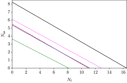
Figure 1: Estimates of the extent of the conformal window in $Sp(4)$ theories coupled to $N_{\rm f}$ Dirac fermions transforming in the fundamental and $N_{\rm as}$ in the 2-index antisymmetric representation. The black solid line denotes the upper bound of the conformal window, while different colored and shaped lines denote alternative analytical estimates of the lower bound, obtained with different approximations. The dashed line is obtained by imposing the constraint $b_{2}(N_{\rm f},\,N_{\rm as})=0$. The dot-dashed line is the result of the all-order beta function with the assumption that the anomalous dimensions of the fermion bilinears are $\gamma_{\bar{\Psi}\Psi}=\gamma_{\bar{Q}Q}=1$. The dotted line is the result of the SD analysis. The BZ expansion leads to the lower (blue) solid line. Details about these approximations can be found in the main text and in the reference list.

More recently, the scheme-independent BZ expansion in the small parameter $\Delta_{N_{\rm{as}}}=N_{\rm{as}}^{\rm AF}-N_{\rm{as}}^{\rm IR}$ has been extensively applied to the determination of physical quantities such as the anomalous dimension, $\gamma_{\bar{\psi}\psi}$, at the IR fixed point—see Ref. Ryttov:2017kmx and refs. therein. In Ref. Kim:2020yvr , the authors determined the lower edge of the conformal window by imposing the critical condition of $\gamma_{\bar{\psi}\psi}(2-\gamma_{\bar{\psi}\psi})=1$. This condition is identical to $\gamma_{\bar{\psi}\psi}=1$ at infinite order, but displays better convergence at finite order in the $\Delta_{N_{\rm{as}}}$ expansion. The 4th order calculation yields $N_{\rm as}^{\gamma cc,\,{\rm cr}}\simeq 5.5$ for $Sp(4)$ Lee:2020ihn .

These analytical approaches can be extended to determine the conformal window for the theory containing fermions in the multiple representations, $\{R_{1},\,R_{2},\,\cdots,\,R_{k}\}$, in which case the upper and lower bounds of the conformal window are described by $(k-1)$-dimensional hyper-surfaces. For the $Sp(4)$ theories of interest with $N_{\rm f}$ Dirac fermions transforming in the fundamental and $N_{\rm as}$ in the 2-index antisymmetric representation, the results are summarised in Fig. 1. The upper bound is determined by the condition $b_{1}(N_{\rm f},\,N_{\rm as})=0$. The various alternative determinations of the lower bound are estimated as follows. The dashed line is obtained by setting $b_{2}(N_{\rm f},\,N_{\rm as})=0$. The dot-dashed line corresponds to the result of the all-order beta function with the input of $\gamma_{\bar{\Psi}\Psi}=\gamma_{\bar{Q}Q}=1$. The dotted and solid lines are the results of the SD analysis and the BZ expansion of $\gamma_{\bar{\Psi}\Psi}$ at the 3rd order in $\Delta_{N_{\rm f}(n_{\rm as})}$ Ryttov:2018uue with the critical conditions applied to the antisymmetric fermions, $\alpha_{\rm BZ}=\alpha^{\rm cr}_{\rm as}=\pi/3C_{2}({\rm AS})$ and $\gamma_{\bar{\Psi}\Psi}(2-\gamma_{\bar{\Psi}\Psi})=1$, respectively, as fermions in the higher representation are expected to condense first, resulting in the larger values of $\alpha^{\rm cr}$ and $\gamma_{\rm IR}$ Ryttov:2010hs . It might be possible to make use of the five-loop computations in Refs. Herzog:2017ohr ; Baikov:2016tgj , to further improve these estimations of the conformal window, but this goes beyond the purposes of this discussion. For the purpose of phenomenological applications, the most interesting physical quantities one would like to determine within the conformal window are the anomalous dimensions of fermion bilinear operators (mesons) and chimera baryon operators. Perturbative calculations of the former are available in the literature, up to the 4th order of the coupling expansion Chetyrkin:2016ruf and at the 3rd order of the BZ expansion Ryttov:2018uue , while that of the latter is only available at the leading order in $\alpha$ BuarqueFranzosi:2019eee . All of these considerations, summarised in Fig. 1, offer some intuitive guidance for what can be expected, but non-perturbative instruments are needed to test these predictions and put Fig 1 on firmer grounds.

II.2 The lattice theory

In presenting the lattice theory, we borrow again notation and conventions from Ref. Bennett:2022yfa . The theory is defined on a Euclidean, hypercubic, four-dimensional lattice with spacing $a$, with $L/a$ sites in the space directions and $T/a$ in the time direction. The generic lattice site is denoted as $x$, and the link in direction $\mu$ as $(x,\,\mu)$. The total number of sites is thus $\tilde{V}/a^{4}=T\times L^{3}/a^{4}$. Unless stated otherwise, in the following we set $L=T$. The action is the sum of two terms

$$S\equiv S_{g}+S_{f}\,,$$ (13)

where $S_{g}$ and $S_{f}$ are the gauge and fermion action, respectively. Among the several choices for the former–the Iwasaki, Symanzik, DBW2 and Wilson gauge actions–for simplicity, we show our results using the Wilson action, defined as

$$S_{g}\equiv\beta\sum_{x}\sum_{\mu<\nu}\left(1-\frac{1}{2N}{\rm Re}\,{{\rm Tr}}\,{\cal P}_{\mu\nu}(x)\right),$$ (14)

where ${\cal P}_{\mu\nu}(x)\equiv U_{\mu}(x)U_{\nu}(x+\hat{\mu})U_{\mu}^{\dagger}(x+\hat{\nu})U_{\nu}^{\dagger}(x)$ is known as the elementary plaquette operator, $U_{\mu}(x)\in Sp(2N)$ is the link variable defined on link $(x,\mu)$, and $\beta\equiv 4N/g_{0}^{2}$, where $g_{0}$ is the bare gauge coupling. For the fermions, we adopt the massive Wilson-Dirac action,

$$S_{f} \equiv a^{4}\sum_{j=1}^{N_{\rm f}}\sum_{x}\overline{Q}^{j}(x)D^{\mathrm{(f)}}_{m}Q^{j}(x)+a^{4}\sum_{j=1}^{N_{\rm as}}\sum_{x}\overline{\Psi}^{j}(x)D^{\mathrm{(as)}}_{m}\Psi^{j}(x)\,,$$ (15)

where $Q^{j}$ and $\Psi^{j}$ are the fermion fields transforming, respectively, in the fundamental and 2-index antisymmetric representation and $j$ is a flavor index, while color and spinor indices are omitted for simplicity. The massive Wilson-Dirac operators in Eq. (15) are defined as

$$D^{\mathrm{(f)}}_{m}Q^{j}(x) \equiv (4/a+m^{\mathrm{f}}_{0})Q^{j}(x)$$

$$-\frac{1}{2a}\sum_{\mu}\left\{(1-\gamma_{\mu})U^{\mathrm{(f)}}_{\mu}(x)Q^{j}(x+\hat{\mu})+(1+\gamma_{\mu})U^{\mathrm{(f)},\,\dagger}_{\mu}(x-\hat{\mu})Q^{j}(x-\hat{\mu})\frac{}{}\right\}\,,$$

and

$$D^{\mathrm{(as)}}_{m}\Psi^{j}(x) \equiv (4/a+m^{\mathrm{as}}_{0})\Psi^{j}(x)$$

$$-\frac{1}{2a}\sum_{\mu}\left\{(1-\gamma_{\mu})U^{\mathrm{(as)}}_{\mu}(x)\Psi^{j}(x+\hat{\mu})+(1+\gamma_{\mu})U^{\mathrm{(as)},\,\dagger}_{\mu}(x-\hat{\mu})\Psi^{j}(x-\hat{\mu})\frac{}{}\right\}\,,$$

where $m_{0}^{\mathrm{f}}$ and $m_{0}^{\mathrm{as}}$ are the bare fermion masses in the fundamental and $2$-index antisymmetric representation, and $U^{\mathrm{(f)}}_{\mu}(x)=U_{\mu}(x)$. The link variables $U^{\mathrm{(as)}}_{\mu}(x)$ are defined as in Ref. Bennett:2022yfa , as follows:

$$U^{\mathrm{(as)}}_{\mu,\,(ab)(cd)}={\rm Tr}\left(e^{(ab)\,T}U^{(\rm f)}_{\mu}e^{(cd)}U^{(\rm f)\,T}_{\mu}\right)\,,$$ (18)

where $e^{(ab)}$ are the elements of an orthonormal basis in the $(N(2N-1)-1)$-dimensional space of $2N\times 2N$ antisymmetric and $\Omega$-traceless matrices, and the multi-indices $(ab)$ run over the values $1\leq a<b\leq 2N$. The entry $ij$ of each element of the basis is defined as follows. For $b\neq N+a$,

$$e^{(ab)}_{ij}\equiv\frac{1}{\sqrt{2}}\left(\delta_{aj}\delta_{bi}-\delta_{ai}\delta_{bj}\right)\;,$$ (19)

while for $b=N+a$ and $2\leq a\leq N$,

$$e^{(ab)}_{i,i+N}=-e^{(ab)}_{i+N,i}\equiv\begin{cases}\frac{1}{\sqrt{2a(a-1)}}\;,\;\;\;\text{for}\;\;i<a\,,\\ \frac{1-a}{\sqrt{2a(a-1)}}\;,\;\;\;\text{for}\;\;i=a\,.\end{cases}$$ (20)

It is easy to verify that each element of this basis satisfies the $\Omega$-traceless condition ${\rm Tr}(e^{(ab)}\Omega)=0$, where the symplectic matrix $\Omega$ is defined in Eq. (43).

Finally, we impose periodic boundary conditions on the lattice for the link variables, while for the fermions we impose periodic boundary conditions along the space-like directions, and anti-periodic boundary conditions along the time-like direction.

III Numerical Implementation: Grid

Our numerical studies are performed using Grid Boyle:2015tjk ; Boyle:2016lbp ; Yamaguchi:2022feu : a high level, architecture-independent, C++ software library for lattice gauge theories. The portability of its single source-code across the many architectures that characterise the exascale platform landscape makes it an ideal tool for a long-term computational strategy. Grid has already been used to study theories based on $SU(N_{c})$ gauge groups with $N_{c}\geq 3$, and fermions in multiple representations Cossu:2019hse ; DelDebbio:2022qgu . In this section, we describe the changes that have been implemented in Grid in order to enable the sampling of $Sp(2N)$ gauge field configurations. With the aim of including dynamical fermions in future explorations of $Sp(2N)$ gauge theories, we focused our efforts on the Hybrid Monte Carlo (HMC) algorithm and on its variation, the Rational HMC (RHMC), used whenever the number of fermion species is odd.

The (R)HMC algorithms generate a Markov chain of gauge configurations distributed as required by the lattice action described in Sect. II.2. The ideas underpinning these two algorithms can be summarized as follows. Firstly, bosonic degrees of freedom $\phi$ and $\phi^{\dagger}$, known as pseudofermions, are introduced replacing a generic number $n_{f}$ of fermions. Powers of the determinant of the hermitian Dirac operator, $Q^{R}_{m}=\gamma_{5}D^{R}_{m}$, in representation $R$ can then be expressed as

$$(\det{D^{R}_{m}})^{n_{f}}=(\det{Q^{R}_{m}})^{n_{f}}=\int\mathcal{D}\phi\mathcal{D}\phi^{\dagger}e^{-a^{4}\sum_{x}\phi^{\dagger}(x)(Q^{2}_{m})^{-n_{f}/2}\phi(x)}~{},$$ (21)

where flavor and color indices of $\phi$ and $\phi^{\dagger}$ have been suppressed for simplicity. For odd values of $n_{f}$, the rational approximation is used to compute odd powers of the determinant above, resulting in the RHMC.

Second, a fictitious classical system is defined, with canonical coordinates given by the elementary links and Lie-algebra-valued conjugate momenta $\pi(x,\,\mu)=\pi^{a}(x,\,\mu)\,t^{a}$, where $t^{a}$ are the generators of the $\mathfrak{sp}(2N)$ algebra in the fundamental representation. The fictitious hamiltonian is

$$H=\frac{1}{2}\sum_{x,\mu,a}\pi^{a}(x,\,\mu)\pi^{a}(x,\,\mu)+H_{g}+H_{f}\,,$$ (22)

where $H_{g}=S_{g}$ and $H_{f}=S_{f}$. The molecular dynamics (MD) evolution in fictitious time $\tau$ is dictated by

$$\frac{\mathrm{d}U_{\mu}(x)}{\mathrm{d}\tau}=\pi(x,\,\mu)U_{\mu}(x)~{},\quad\frac{\mathrm{d}\pi(x,\,\mu)}{\mathrm{d}\tau}=F(x,\mu)\,,$$ (23)

where $F(x,\mu)$, known as the HMC force, is defined on the Lie algebra $\mathfrak{sp}(2N)$, and can be expressed as $F(x,\,\mu)=F_{g}(x,\,\mu)+F_{f}(x,\,\mu)$. The detailed form for $F_{g}(x,\,\mu)$ and $F_{f}(x,\,\mu)$ DelDebbio:2008zf , the gauge and fermion force can be found in Section IIIA of Ref. DelDebbio:2008zf .
Numerical integration of the MD equations thus leads to a new configuration of the gauge field, which is then accepted or rejected according to a Metropolis test. The update process can hence be described as follows:

• pseudofermions distributed according to the integrand in Eq. (21) are generated with the Heat Bath algorithm,

• starting with Gaussian random conjugate momenta, the MD equations in Eqs. (23) are integrated numerically,

• the resulting gauge configuration is accepted or rejected by a Metropolis test.

In this section we provide details on the implementation of the operations listed above, focusing on the alterations made to the pre-existing structure of the code designed for $SU(N_{c})$ gauge theories. We then describe and carry out three types of technical checks, following Ref. DelDebbio:2008zf . We test the behaviour of the HMC and RHMC algorithms. We produce illustrative examples of the behaviour of the molecular dynamics (MD). Finally, we carry out a comparison between HMC and RHMC algorithms. The purpose of these tests is to verify that the dynamics is implemented correctly.

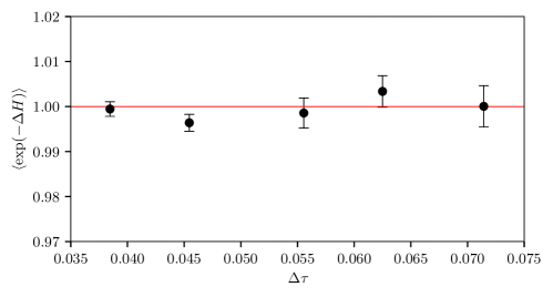
Figure 2: Test of Creutz equality, $\langle\exp(-\Delta H)\rangle=1$; dependence of $\langle\exp(-\Delta H)\rangle$ on the time–step $\Delta\tau$ in the MD integration, for $N=2$, $N_{\rm f}=0$, and $N_{\rm as}=4$. The relevant parameters of this study are the trajectory length $\tau=1$, number of steps $n_{\rm steps}=14,16,18,22,26$ ($\Delta\tau=\tau/n_{\rm steps}$), for an ensemble with lattice volume $\tilde{V}/a^{4}=8^{4}$, $\beta=6.8$, and $am_{0}^{\rm as}=-0.6$.

III.1 Software development

As in the case for the pre-existing routines handling the theories with gauge group $SU(N_{c})$, our implementation of $Sp(2N)$ allows for a generic number of colors. The starting point of the MD is the generation of random Lie-algebra-valued conjugate momenta. The generators of the $\mathfrak{sp}(2N)$ Lie Algebra in the fundamental representation, as they appear in Grid, are provided by the relations described in Appendix B, where conventions for their normalisation are also established. Generators in higher representations of the gauge group can be derived from the fundamental ones DelDebbio:2008zf ; Cossu:2019hse . In particular, the generators of the algebra of $Sp(2N)$ in the antisymmetric representation can be obtained from the definition in Eq. (18), by Taylor expanding to first order around the unit transformation,

$$(t_{\mathrm{as}}^{a})_{(ab)(cd)}={\rm Tr}\left(e^{(ab)\,T}t_{\mathrm{f}}^{a}e^{(cd)}+e^{(ab)\,T}e^{(cd)}t_{\mathrm{f}}^{a\,T}\right)\;.$$ (24)

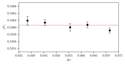
Figure 3: Test of independence of the plaquette on the time–step $\Delta\tau$ used for the MD integration, for $N=2$, $N_{\rm f}=0$, and $N_{\rm as}=4$. The relevant parameters of this study are the trajectory length $\tau=1$, number of steps $n_{\rm steps}=14,16,18,22,26$, $\Delta\tau=\tau/n_{\rm steps}$, for an ensemble with lattice volume $\tilde{V}/a^{4}=8^{4}$, $\beta=6.8$, and $am_{0}^{\rm as}=-0.6$. The horizontal line corresponds to the plaquette value obtained averaging over trajectories having different a number of step values, $n_{\rm steps}$.

In the numerical integration of Eq. (23), it is required to project the HMC force on the Lie algebra of the gauge group. In Grid, the embedding of the force-projection within the integrator requires the forces to be anti-hermitian. Hence, a projection operation to the matrices of the algebra $\mathfrak{sp}(2N)$ must be defined. This can be done in analogy with the projection to $\mathfrak{su}(N_{c})$, defined for a generic matrix $M$ as

$$P_{\text{tr}}P_{\text{aH}}M\;,$$ (25)

where $P_{\text{tr}}M\equiv M-\mathbb{1}_{N_{c}}\mathrm{Tr}(M)/N_{c}$ and $P_{\text{aH}}M\equiv(M-M^{\dagger})/2$ are the projectors to its traceless and to its anti-hermitian parts, respectively. For $\mathfrak{sp}(2N)$, the projection is instead defined as,

$$P_{\text{aH}}P^{-}_{\text{Sp}}P_{\text{tr}}\,M\;,$$ (26)

where

$$P^{\pm}_{\text{Sp}}M\equiv\frac{M\pm\Omega M^{*}\Omega}{2}\;.$$ (27)

Notice that $P^{-}_{\text{Sp}}$ returns an anti-hermitian matrix, while $P^{+}_{\text{Sp}}$ projects on a space of hermitian matrices.

The resympleticisation of gauge links to the $Sp(2N)$ group manifold has also been implemented in Grid. The algorithm Bennett:2017kga is a modification of the Gram-Schmidt process designed to take into account the condition in Eq. (45). After normalising the first column of the matrix $U$, the $(N+1)$-th column is set to

$$\mathrm{col}(U)_{j+N}=-\Omega\,\mathrm{col}(U)_{j}^{*}\;.$$ (28)

The second column is then obtained by orthonormalisation with respect to both the first and the $N+1$-th column. An iteration of this process leads to a $Sp(2N)$ matrix. This procedure, performed after every update, prevents the gauge fields from drifting away from the group manifold due to the finite precision of the simulation.

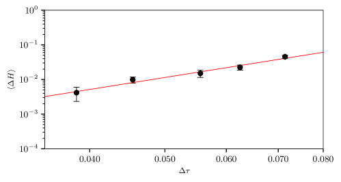
Figure 4: Dependence of $\langle\Delta H\rangle$ on the time-step, $\Delta\tau$, used for the MD integration, for $N=2$, $N_{\rm f}=0$, and $N_{\rm as}=4$. The expectation value $\langle\Delta H\rangle$ is proportional to $(\Delta\tau)^{4}$, consistently with the use of a second-order integrator. The plot is shown in log-log scale. The relevant parameters of this study are the trajectory length $\tau=1$, number of steps $n_{steps}=14,16,18,22,26$ ($\Delta\tau=\tau/n_{\textnormal{steps}}$), for an ensemble with lattice volume $\tilde{V}/a^{4}=8^{4}$, $\beta=6.8$, and $am_{0}=-0.6$.

III.2 Basic tests of the algorithm

In this subsection, we follow closely Sects. III and IV of Ref. DelDebbio:2008zf . Our MD evolution is implemented using a second-order Omelyan integrator Takaishi:2005tz . However, in this work, the inversion of the fermion matrix is treated without preconditioning DeGrand:1990dk ; Bennett:2022yfa .

We now restrict attention to the theory with $N=2$, $N_{\rm f}=0$, and $N_{\rm as}=4$, and perform a set of preliminary checks on the algorithms we use. We present the results in Figs. 2, 3, 4, 5, and 6, obtained, for convenience, setting the lattice parameters to $\beta=6.8$, and $am_{0}=-0.6$, on an isotropic lattice with volume $\tilde{V}=(8a)^{4}$.

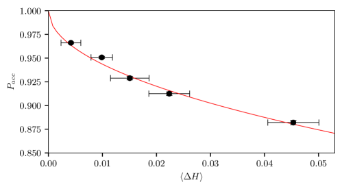
Figure 5: Test of the relation between acceptance probability and $\Delta H$, for $N=2$, $N_{\rm f}=0$, and $N_{\rm as}=4$. The expected behaviour $P_{acc}=\hbox{erfc}(\sqrt{\Delta H}/2)$ is supported. The relevant parameters of this study are the trajectory length $\tau=1$, number of steps $n_{\rm steps}=14,16,18,22,26$ ($\Delta\tau=\tau/n_{\rm steps}$), for an ensemble with lattice volume $\tilde{V}/a^{4}=8^{4}$, $\beta=6.8$, and $am_{0}=-0.6$.

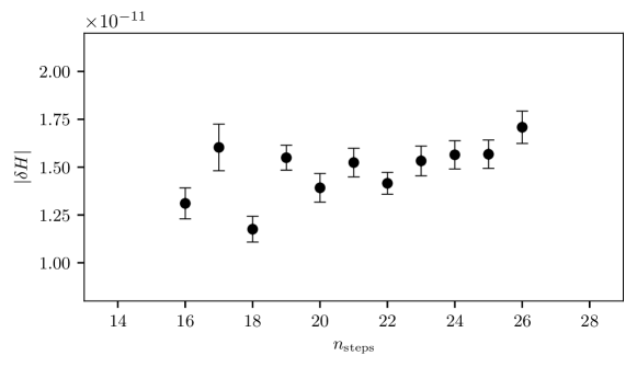
Figure 6: Reversibility test, showing $|\delta H|$ for various choices of $\Delta\tau$, for $N=2$, $N_{\rm f}=0$, and $N_{\rm as}=4$. The relevant parameters of this study are the trajectory length $\tau=1$, number of steps $n_{\rm steps}\in[16,26]$ ($\Delta\tau=\tau/n_{\rm steps}$), for an ensemble with lattice volume $\tilde{V}/a^{4}=8^{4}$, $\beta=6.8$, and $am_{0}=-0.6$.

The first test pertains to Creutz equality Creutz:1988wv : by measuring the difference in Hamiltonian, $\Delta H$, evaluated before and after the MD evolution, one should find that

$$\left\langle\exp\left(-\frac{}{}\Delta H\right)\right\rangle = 1\,.$$ (29)

This is supported by our numerical results: Fig. 2 shows the value of $\left\langle\exp\left(-\frac{}{}\Delta H\right)\right\rangle$ for five different choices of the time-step used in the MD integration, with $\Delta\tau=\tau/n_{steps}$, and the choice $\tau=1$. The numerical results are obtained by considering a thermalised ensemble consisting of $3400$ trajectories, that we find has integrated auto-correlation time $\tau_{c}=6.1(2)$, measured using the Madras-Sokal windowing process Madras:1988ei . A closely related test is shown in Fig. 3: the value of the ensemble average of the plaquette is independent of $\Delta\tau$.

A third test pertains to the dependence of $\langle\Delta H\rangle$ on $\Delta\tau$, which for a second-order integrator is supposed to scale as $\langle\Delta H\rangle\propto(\Delta\tau)^{4}$ Takaishi:1999bi . In Fig. 4 we show our measurements, together with the result of a best-fit to the curve $\log\langle\Delta H\rangle={\cal K}_{1}\,\log(\Delta\tau)+{\cal K}_{2}$, with ${\cal K}_{1}=3.6(4)$ determined by minimising a simple $\chi^{2}$. We find good agreement, as quantified by the value of the reduced $\chi^{2}/N_{\rm d.o.f.}=0.6$, and ${\cal K}_{1}$ is compatible to $4$. A closely related test is displayed in Fig. 5, confirming the prediction that the acceptance probability of the algorithm, $P_{\rm acc}$, obeys the relation Gupta:1990ka :

$$P_{\rm acc} = {\rm erfc}\left(\frac{1}{2}\sqrt{\left\langle\Delta\frac{}{}H\right\rangle}\right)\,.$$ (30)

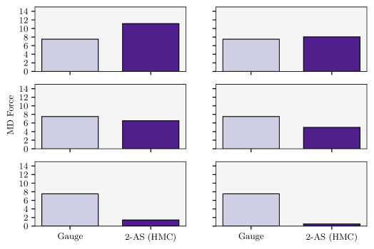
Figure 7: Field contribution to the MD force for the theory with $N=2$, $N_{\rm f}=0$, and $N_{\rm as}=4$, on isotropic lattice with $\tilde{V}=(8a)^{4}$, and lattice coupling $\beta=6.8$. The two blocks are respectively indicating the gauge (light shading, left) and the fermion (dark shading, right) contribution, the latter computed with the HMC algorithm. Fermion contributions are summed over flavor. The six panels correspond to different choices of bare mass: $am_{0}^{\rm as}=-0.9,\,-0.1,\,+0.6,\,+1.8,\,+15,\,+50$ (left to right, top to bottom).

The final test of this subsection is displayed in Fig. 6. Following Refs. DelDebbio:2008zf ; Joo:2000dh , we also want to ensure that the reversibility of our updates is respected. Reversibility is one of the fundamental properties required in order to pursue a correct HMC update. Our update algorithm, based on leapfrog, is reversible analytically. Yet, when using this algorithm numerically on computers, because of the finite precision, exact reversibility is lost. It is therefore important to verify that implementation of the fundamental steps of the algorithm can be considered as reversible to good approximation, in order to avoid that rounding errors introduce a significant bias in our calculations. One can show that the quantity $|\delta H|$—the average difference of the Hamiltonian evaluated by evolving the MD forward and backward and flipping the momenta at $\tau=1$—doesn’t change significantly in our simulations. Since the Hamiltonian in these tests is of order $\sim 10^{6}$ and the typical $\delta H\sim 10^{-11}$, the results show that the violation of reversibility is consistent with having $|\delta H|/H$ of the order of the numerical accuracy. This is the expected relative precision for double-precision floating-point numbers. Moreover, the violation $|\delta H|$ is independent of $\Delta\tau$. As a “microscopic” and related effect, reversibility violations may occur while updating the gauge link variables and momenta updates during the MD evolution. To ensure this doesn’t occur we update the gauge links through the exponentiation of the momenta, so that $U(\pi)\,U(-\pi)=1$. Moreover, thanks to the double-precision nature of the variables we use, the entity of relative violations for momenta results to be within machine-accuracy in our simulations, as in the global reversibility violation case.

III.3 More about the Molecular Dynamics

Figure 8: Compatibility between plaquette averages $\langle P\rangle$ obtained with HMC and RHMC algorithms for the theory with $N=2$, $N_{\rm f}=0$, and $N_{\rm as}=4$. $\langle P\rangle_{\rm HMC}$ is obtained running two couples of fermions with HMC. For $\langle P\rangle_{\rm RHMC}$ (top panel), RHMC was applied individually to each of the fermions. $\langle P\rangle_{\rm 2HMC+2RHMC}$ (bottom panel) is obtained running two fermions with HMC, while the other two were run with RHMC. The lattice coupling is $\beta=6.8$, with the bare mass in the range $-1.4\leq am^{\rm as}_{0}\leq 0.0$. The lattice is isotropic and has volume $\tilde{V}=(8a)^{4}$.

For illustration purposes, we find it useful to monitor the contribution to the MD of the fields, and how this changes as we dial the lattice parameters. We focus on the theory with $N=2$, $N_{\rm f}=0$, and $N_{\rm as}=4$, and consider a few ensembles with isotropic lattice with $\tilde{V}=(8a)^{4}$, and lattice coupling $\beta=6.8$, but vary the mass $am_{0}^{\rm as}$. We show in Fig. 7 the force, $F$, as defined in Eq. (23), split in its contribution from the gauge and fermion dynamics, the latter computed using the HMC for all fermions. The results are normalised so that the gauge contribution is held constant. As can be clearly appreciated, for large and positive values of $am_{0}^{\rm as}$ the fermions can be neglected, as for these choices of the mass, one expects to be in the quenched regime. When decreasing the mass, the fermion contribution increases. For large, negative values of the Wilson bare mass (close to the chiral limit), the fermion contribution is even larger than the contribution of the gauge part of the action.

III.4 Comparing HMC and RHMC

While in this paper we are mostly interested in the theory with $N=2$, $N_{\rm f}=0$, and $N_{\rm as}=4$, and hence we can use the HMC algorithm, for the general purpose of identifying the extent of the conformal window in this class of lattice gauge theories it may be necessary to consider also odd numbers of fermions, for which we resort to the RHMC algorithm. The latter relies on a rational approximation in the computation of the fermion force, but the presence of a Metropolis accept-reject step ensures that the algorithm is exact. Thus, a preliminary test must be made to check the consistency of the implementation—as was done for $SU(3)$ theories, see for instance Ref. Clark:2003na . To gauge whether the numerical implementation is working at the desired level of accuracy and precision, we performed the exercise leading to Fig. 8. We computed the average plaquette, $\langle P\rangle$, where $P$ is defined as

$$P\equiv\dfrac{a^{4}}{6\tilde{V}}\sum_{x}\sum_{\mu<\nu}\left[\frac{1}{2N}{\rm Re}\,{{\rm Tr}}\,{\cal P}_{\mu\nu}(x)\right]$$ (31)

for ensembles having lattice volume $\tilde{V}=(8a)^{4}$ and coupling $\beta=6.8$, for a few representative choices of the bare mass $-1.4\leq am^{\rm as}_{0}\leq 0.0$. We repeated this exercise three times: at first, we treated all fermions with the HMC, then we treated them all with the RHMC, and finally we used a mixed strategy, treating two fermions with the HMC, and two with the RHMC. We display, in the two plots in the figure, the differences of the second and third approaches to the first one, respectively. For most of the data, the differences are compatible with zero within the statistical uncertainties. More generally, given the number of observables, the probability to find a deviation larger than $3\sigma$ from the null value results to be $\sim 12\%$.

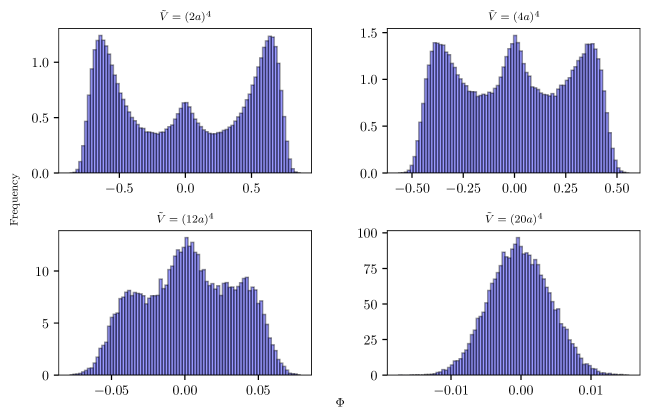
Figure 9: Study of finite-size effects on the lattice, for the $Sp(4)$ Yang-Mills theory. The histograms depict the distribution of (real) Polyakov loops for ensembles with $\beta=9.0$ and four choices of space-time volume: $\tilde{V}=(2a)^{4},\,(4a)^{4},\,(12a)^{4},\,(20a)^{4}$. The histograms’ areas are normalised to $1$.

IV The $N=2$ lattice Yang-Mills theory

In this section, we start to analyse the physics of the $Sp(4)$ theory of interest. We begin from the pure Yang-Mills dynamics, with $N_{\rm f}=0=N_{\rm as}$. We verify that centre symmetry, $\left({\mathbb{Z}}_{2}\right)^{4}$, is broken at small volumes, but restored at large volumes, by looking at the (real) Polyakov loop, in a way that is reminiscent of Ref. Athenodorou:2014eua . Following Ref. Cossu:2019hse , we then consider the spectrum of the Dirac operator in the quenched approximation, both for fundamental and 2-index antisymmetric fermions, to verify the symmetry-breaking pattern expected from random matrix theory.

The results for the first of these tests are shown in Fig. 9. At a coupling $\beta=9.0$, we generate four ensembles in the pure $Sp(4)$ theory, at different values of the space-time volume, $\tilde{V}=(2a)^{4},\,(4a)^{4},\,(12a)^{4},\,(20a)^{4}$. For each configuration, we compute the spatial averaged (real) Polyakov loop, defined as

$$\Phi \equiv \frac{1}{N_{c}N_{s}^{3}}\sum_{\vec{x}}{\rm Tr}\left(\prod_{t=0}^{t=N_{t}-1}U_{0}(t,\vec{x})\right)\,,$$ (32)

where $U_{0}(t,\vec{x})$ is the time-like link variable. For our current purposes, we choose the lattice to be isotropic in all four directions, $N_{t}=N_{s}=L/a$. For each ensemble, we display the frequency histogram of the values of $\Phi$. The expectation is that the zero-temperature $Sp(4)$ lattice theory should preserve the $\left({\mathbb{Z}}_{2}\right)^{4}$ symmetry of the centre of the group in four Euclidean space-time dimensions. This is indeed the case for sufficiently large volumes, as shown by the bottom-right panel of Fig. 9, for which $N_{t}=N_{s}=20$, that exhibits a Gaussian distribution centred at the origin. But for small enough lattice volumes, this expectation is violated. This is visible in the other three panels in Fig. 9, in which the distribution is non-Gaussian, and two other peaks emerge. In the extreme case of $N_{s}=N_{t}=2$, the two peaks at finite value of $\Phi$ dominate the distribution, which is otherwise symmetrical around zero. Interestingly, Polyakov loops can be used also to perform the more physical study of the finite-temperature confinement/deconfinement phase transition. In this case, one would consider $N_{t}\neq N_{s}$, vary the coupling $\beta$ to identify the transition temperature, and then perform continuum and infinite volume extrapolations. The characterisation of the deconfinement phase transition is of interest for both theoretical as well as phenomenological reasons—see Ref. Holland:2003kg and the review in Ref. Bennett:2023wjw —but requires a dedicated, extensive programme of numerical work, and possibly cutting-edge new technology to address some of the difficulties faced by conventional Monte Carlo sampling methods (see, e.g., the discussions in Refs. Borsanyi:2022xml and Lucini:2023irm ), while the simpler analysis performed here suffices for the more modest purposes of this paper.

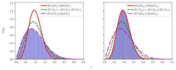
Figure 10: Distribution of the folded density of spacing between subsequent eigenvalues of the hermitian Dirac-Wilson operator $Q_{m}=\gamma_{5}D_{m}$, and comparison with predictions from chRMT, computed in the quenched approximation, with ensembles having $\beta=8.0$, $am_{0}=-0.2$, and lattice volume $\tilde{V}=(4a)^{4}$, in the $Sp(4)$ theory. The left panel shows the case of fermions transforming in the fundamental representation, and the right is for fermions in the 2-index antisymmetric one.

Ensembles of gauge configurations without dynamical fermions can also be used to verify that our implementation of the Dirac operators is correct. To this purpose, following Ref. Cossu:2019hse (and Ref. Bennett:2022yfa ), we consider the theory with quenched fermions in either the fundamental or 2-index antisymmetric representation, and compute the spectrum of eigenvalues of the hermitian Wilson-Dirac operator $Q_{m}=\gamma_{5}D_{m}$. The numbers of configurations are $N_{\rm{conf,f}}=88$ and $N_{\rm{conf,as}}=47$, while the number of eigenvalues in each configuration used is $3696$ for fundamental fermions and $5120$ for antisymmetric fermions. Then, we compute the distribution of the folded density of spacing, $P(s)$. Finally, we compare the results to the exact predictions of chiral Random Matrix Theory (chRMT) Verbaarschot:1994qf ; Verbaarschot:2000dy . Because the spectrum captures the properties of the theory, in particular the pattern of chiral symmetry breaking Banks:1979yr , the distribution $P(s)$ differs, depending on the symmetry-breaking pattern predicted. The folded density of spacing is

$$P(s)=N_{\tilde{\beta}}s^{\tilde{\beta}}\exp\left(-c_{\tilde{\beta}}s^{2}\right)\,,\quad\hbox{where}\quad N_{\tilde{\beta}}=2\dfrac{\Gamma^{\tilde{\beta}+1}\left(\frac{\tilde{\beta}}{2}+1\right)}{\Gamma^{\tilde{\beta}+2}\left(\frac{\tilde{\beta}+1}{2}\right)},\,c_{\tilde{\beta}}=\dfrac{\Gamma^{2}\left(\frac{\tilde{\beta}}{2}+1\right)}{\Gamma^{2}\left(\frac{\tilde{\beta}+1}{2}\right)}\,,$$ (33)

where $\tilde{\beta}$ is the Dyson index. This index can take three different values: $\tilde{\beta}=2$ corresponds to the symmetry breaking pattern $SU(N_{f})\times SU(N_{f})\to SU(N_{f})$, $\tilde{\beta}=1$ to $SU(2N_{f})\to Sp(2N_{f})$, and $\tilde{\beta}=4$ to $SU(2N_{f})\to SO(2N_{f})$. The latter two are the cases we are interested in, corresponding to fundamental and 2-index antisymmetric fermions for the symplectic theory.

In order to make a comparison with the chRMT prediction in Eq. (33), we compute the eigenvalues of $Q_{m}$ for $N_{\rm conf}$ configurations. This process yields a set of eigenvalues $\lambda^{(c)}_{i}$ with $c=1,\cdots,N_{\rm conf}$. The eigenvalues are arranged in one long list, in which $\lambda^{(c)}_{i}$ are ordered in ascending order. Any degeneracy that is present in the 2-antisymmetric case is discarded. Then, for each $c=1,\cdots,N_{\rm conf}$, a new list of values is produced, that contains $n^{(c)}_{i}$, the positive integer position of the eigenvalue $\lambda^{(c)}_{i}$ in the long list ordered in ascending order, instead of $\lambda^{(c)}_{i}$. The density of spacing, $s$, is replaced by the expression

$$s=\dfrac{n^{(c)}_{i+1}-n^{(c)}_{i}}{\mathcal{N}}\,.$$ (34)

The constant $\mathcal{N}$ is defined so that the density of spacing has unit average over the whole ensemble, $\langle s\rangle=1$. Finally, the (discretised) unfolded density of spacings, $P(s)$, is obtained by binning numerical results for $s$ and normalising it.

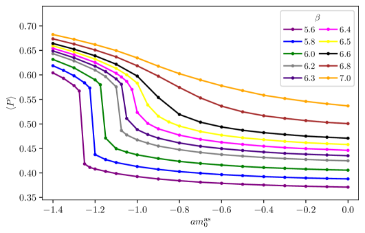
Figure 11: Parameter scan of the $Sp(4)$ theory with $N_{\rm as}=4$ fermions transforming in the 2-index antisymmetric representation, with ensembles generated from a cold start, using the HMC. We show the value of the average plaquette, $\langle P\rangle$, as a function of the bare mass, for a few representative values of the coupling. The lattice size is $\tilde{V}=(8a)^{4}$, and each point is obtained by varying the lattice coupling $\beta=7.0,6.8,6.6,6.5,6.4,6.3,6.2,6.0,5.8,5.6$ and the bare mass $-1.4\leq am_{0}^{\rm as}\leq 0.0$.

In Fig. 10, we show an example of the folded distribution of eigenvalues of the Wilson-Dirac operator, computed numerically. As it can be seen, in the case of fermions in the fundamental representation, one finds a distribution that is compatible with the symmetry breaking pattern leading to the coset $SU(2N_{\rm f})/Sp(2N_{\rm f})$. Conversely, for fermions in the 2-index antisymmetric representation, our numerical results reproduce the prediction associated with the coset $SU(2N_{\rm as})/SO(2N_{\rm as})$. The spectacular agreement with chRMT confirms that there are no inconsistencies in our way of treating fermions. The size of the lattices we have considered has been chosen in order to reduce finite-size effects. These effects, as shown in Ref. Bennett:2022yfa , can become evident in smaller lattices and they lead to discrepancies due to some abnormally large spacings for the smallest and largest eigenvalues. This was interpreted to be an artefact due to the finiteness of the lattice size. We observe that, as in previous studies, the antisymmetric representation already matches the predictions in a $4^{4}$ volume, while for the fundamental to reproduce the predictions chRMT, we had to remove the $200$ lowest and highest eigenvalues (reducing the number of eigenvalues from $4096$ to $3696$). In this fashion, the differences with chRMT are no longer visible to the naked eye even for lattices with modest volume, $\tilde{V}=(4a)^{4}$.

V The $N=2$ theories coupled to fermions: bulk phase structure

In this section, we present our main results for the theory with $N=2$, $N_{\rm f}=0$, and varying number of fermions transforming in the antisymmetric representation, starting from $N_{\rm as}=4$—for which we apply the HMC algorithm. We performed a coarse scan of the lattice parameter space, to identify phase transitions in the $(\beta,m_{0})$ plane, by studying the average plaquette, $\langle P\rangle$, its hysteresis, and its susceptibility. We provide an approximate estimate of the upper bound coupling for the bulk phase, $\beta_{\ast}$, above which there is no bulk phase transition, and hence one can safely perform lattice numerical calculations at finite lattice spacing, yet confident that the results can be extrapolated to the appropriate continuum limit.

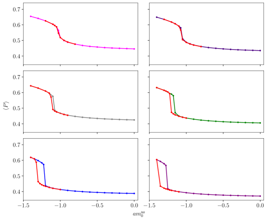
Figure 12: Hysteresis between hot (red) and cold (other colors) starts for the $Sp(4)$ theory with $N_{\rm as}=4$ fermions in the 2-index antisymmetric representation. The lattice coupling is $\beta=6.4,6.3,6.2,6.0,5.8,5.6$ (left to right, and top to bottom). The lattice size is $\tilde{V}=(8a)^{4}$, and each point is obtained by varying the bare mass $-1.4\leq am_{0}^{\rm as}\leq 0.0$.

Figure 11 displays the average plaquette, $\langle P\rangle$, obtained in ensembles generated using a cold start. The lattice size is $\hat{V}=(8a)^{4}$, and each point is obtained by varying the lattice coupling $\beta=7.0,6.8,6.6,6.5,6.4,6.3,6.2,6.0,5.8,5.6$ and the bare mass $-1.4\leq am_{0}^{\rm as}\leq 0.0$. The figure shows that, for small values of $\beta$ and large, negative values of the bare mass, the average plaquette displays an abrupt change at a particular value $am_{0}^{{\rm as}\,\ast}$, while being a smooth, continuous function elsewhere. This is a first indication of the existence of a first-order bulk phase transition.

To better understand whether a first-order phase transition is taking place, we study the effect of adopting two different strategies in the generation of the ensembles, repeating it using of thermalised (hot) starts, and redoing the measurements. Figure 12 shows the comparison of the average plaquette, $\langle P\rangle$, computed for several fixed choices of the coupling $\beta$, while varying the bare mass $-1.4\leq am_{0}^{\rm as}\leq 0.0$. The two curves in the plots represent the behaviour measured in ensembles obtained from a cold and hot start configuration. The effects of hysteresis are clearly visible for $\beta<6.4$ and are an indication of the presence of a first-order phase transition taking place at a critical value of the bare mass $am_{0}^{{\rm as}\,\ast}$.

The final test of the nature of the phase transition is shown in Fig. 13. For illustration purposes, we choose two values of the coupling for which we have evidence of a phase transition ($\beta=6.2$), or of smooth behaviour of $\langle P\rangle$ for all value of $am_{0}^{\rm as}$ ($\beta=6.5$), respectively. We compute the plaquette susceptibility, defined as

$$\chi_{P} \equiv \frac{\tilde{V}}{a^{4}}\left(\langle P^{2}\rangle-\left(\langle P\rangle\right)^{2}\right)\,,$$ (35)

and compare the numerical results obtained with ensembles having two different volumes, $\tilde{V}=(8a)^{4}$ and $\tilde{V}=(16a)^{4}$. The results indicate that the peak height scales as the $4$-volume when $\beta$ is small, in which case the position of the peak also moves to a different value of $am_{0}^{\rm as}$. These are indeed the expected signature of a first order phase transition. For large $\beta$, we observe a shift in values of $am_{0}^{\rm as}$ and no clear and large change in entity for the peak heights between the two volumes. This is a clear indication of a smooth crossover. We hence conclude that, in the theory with $N=2$, $N_{\rm f}=0$, and $N_{\rm as}=4$, there is numerical evidence of a line of first-order phase transitions turning into a crossover at $\beta>\beta_{\ast}=6.4$.

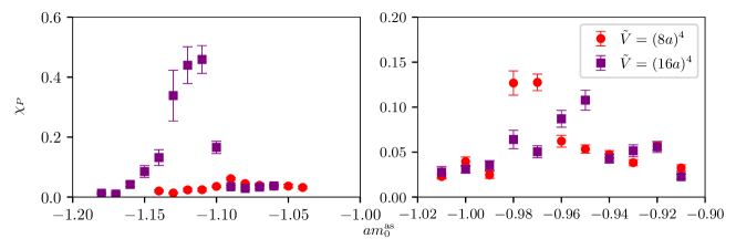
Figure 13: Plaquette susceptibility, $\chi_{P}$, in the $Sp(4)$ lattice theory with $N_{\rm as}=4$ fermions in the 2-index antisymmetric representation. We use two values of the lattice size, $\tilde{V}=(8a)^{4}$ and $\tilde{V}=(16a)^{4}$. The ensembles have $\beta=6.2$, $-1.18\leq am_{0}\leq-1.04$ (left panel), and $\beta=6.5$, $-1.01\leq am_{0}\leq-0.91$ (right panel).

Figure 14: Parameter scan in the $Sp(4)$ theory with $N_{\rm as}=0,\,1,\,2,\,3,\,5,\,6,\,7,\,8$ (left to right and top to bottom panels) fermions in the 2-index antisymmetric representation, obtained with ensembles generated from a cold start. For $N_{\rm as}>0$, we show the value of the average plaquette, $\langle P\rangle$, as a function of the bare mass, for a few representative values of the coupling. For pure gauge, we just vary the value of $\beta$. All the fermions are treated with the HMC/RHMC algorithms. The lattice size is $\tilde{V}=(8a)^{4}$ and the base mass is chosen in the range $-1.4\leq am_{0}^{\rm as}\leq 0.0$ for $N_{\rm as}\geq 2$, and $-1.5\leq am_{0}^{\rm as}\leq 0.0$ for $N_{\rm as}=1$. For the pure gauge theory, the coupling is chosen to be $1.0\leq\beta\leq 16.0$. For $N_{\rm as}=1$, we have chosen $\beta=7.1,7.0,6.9,6.8,6.7,6.6$, while for $N_{\rm as}=2$ we have $\beta=6.8,6.7,6.6,6.5,6.4,6.2$. For $N_{\rm as}=3$, the coupling is $\beta=6.8,6.7,6.6,6.5,6.4,6.2,6.0,5.8$, while for $N_{\rm as}=5$ we’ve chosen $\beta=6.6,6.5,6.4,6.3,6.2,6.1,6.0,5.8$. For $N_{\rm as}=6$, $\beta=6.4,6.3,6.2,6.1,6.0,5.8$. For $N_{\rm as}=7$, $\beta=6.4,6.2,6.1,6.0,5.9,5.8$ and for $N_{\rm as}=8$, $\beta=6.3,6.1,6.0,5.9,5.8,5.7$.

V.1 Varying $N_{\rm as}$

We repeat the parameter scan for other choices of $N_{\rm as}$, using the RHMC for all fermions when $N_{\rm as}$ is odd, and the HMC algorithm otherwise. The purpose of the exercise is to study the dependence of the upper bound coupling for the bulk phase $\beta_{\ast}$ on the number of fermions, $N_{\rm as}$. Indeed, it is expected that for small $N_{\rm as}$ we expect the theory to confine, while for larger values of $N_{\rm as}\sim N_{\rm as}^{c}$ the theory should approach the lower end of the conformal window, and eventually lose asymptotic freedom—we recall that the latter requires to impose the bound $N_{\rm as}<33/4$ in $Sp(4)$, while setting the stage for a first truly non-perturbative determination of the former is the main motivation for this study.

The results of these studies are shown in Fig. 14, which displays our measurements of the average plaquette, $\langle P\rangle$, as a function of the bare parameters of the theories. For the pure gauge $Sp(4)$ theory, we get plaquette values that are in agreement with the ones shown in Ref. Holland:2003kg . The corresponding upper bound value of the coupling is roughly estimated to be $\beta_{\ast}\simeq 7.2$.

For theories with dynamical fermions, we vary both the masses and the coupling of the theories. As can be seen from Fig 14, for $N_{\rm as}=1$ the upper bound is $\beta_{\ast}\simeq 6.7$. For $N_{\rm as}=2$ the upper bound is $\beta_{\ast}\simeq 6.7$, and for $N_{\rm as}=3$ it is $\beta_{\ast}\simeq 6.5$, in agreement with the values found in Ref. Lee:2018ztv . At a larger number of fermions species, we obtain progressively smaller values of $\beta$ for the upper bound of the bulk phase $\beta$: for $N_{\rm as}=5$, we get $\beta_{\ast}\simeq 6.3$. For $N_{\rm as}=6$, the upper bound coupling is $\beta_{\ast}\simeq 6.2$. For $N_{\rm as}=7$, we get $\beta_{\ast}\simeq 6.1\div 6.2$ and for $N_{\rm as}=8$, $\beta_{\ast}\simeq 6.1$.
Overall, we notice a trend according to which the more fermion flavors are present in the $Sp(4)$, the smaller the upper bound value of the coupling we find and the bigger is the corresponding critical bare mass $am_{0}^{\mathrm{(as)}\ast}$.

VI Scale setting and topology

We return now to the theory with $N=2$, $N_{\rm f}=0$, and $N_{\rm as}=4$. We discuss a scale setting procedure that uses the Wilson flow. We also monitor the evolution of the topological charge, to show that topological freezing was avoided. We focus the discussion on a few representative examples, although we checked that our conclusions have general validity for all choices of parameter relevant to this study.

Figure 15: Wilson Flow Luscher:2010iy ; Luscher:2013vga energy density ${\cal E}(t)$ (left panel) and ${\cal W}(t)$ (right), computed as in Refs. Bennett:2017kga ; Bennett:2022ftz , from the standard (pl) and the clover-leaf (cl) plaquette defined in Refs. Sheikholeslami:1985ij ; Hasenbusch:2002ai , for the $Sp(4)$ theory with $N_{\rm as}=4$ fermions transforming in the 2-index antisymmetric representation. The lattice size is $\tilde{V}=(12a)^{4}$, and we display two representative choices of bare parameters, with $\beta=6.8$ or $6.9$ and common bare mass $am_{0}^{\rm as}=-0.8$. The time step is $0.01$, $t_{max}=4.5$ to reduce finite-size effects. Errors are computed by bootstrapping. We have chosen ${\cal W}_{0}=\frac{1}{2}C_{2}(F)$ for the topological charge. The corresponding values of $w_{0}$ from the plaquette and the clover-leaf are $w_{0,pl.}=1.485(3)$ and $w_{0,cl.}=1.495(2)$ for $\beta=6.8$ and $w_{0,pl.}=2.005(2)$ and $w_{0,cl.}=2.026(2)$ for $\beta=6.9$. We have set $a=1$, for notational convenience.

Figure 16: Evolution with the ensemble trajectories of the topological charge $Q_{L}(t=w_{0}^{2})\equiv\sum_{x}\frac{1}{32\pi^{2}}\varepsilon^{\mu\nu\rho\sigma}{\rm Tr}\left[{\cal C}_{\mu\nu}(x){\cal C}_{\rho\sigma}(x)\right]$, computed (without rounding) at flow time $t=w_{0}^{2}$ for the $Sp(4)$ theory with $N_{\rm as}=4$ fermions transforming in the 2-index antisymmetric representation. The lattice size is $\tilde{V}=(12a)^{4}$. The lattice parameters characterising the ensembles are $\beta=6.8$ (top panel) and $\beta=6.9$ (bottom), with bare mass $am_{0}^{\rm as}=-0.8$. The histograms of the measurements (right panels) are compatible with a normal distribution centered at zero, with reduced chi-square $\chi^{2}/N_{\rm d.o.f}=\tilde{\chi}^{2}=1.1$ for both panels. The integrated autocorrelation time computed using the Madras-Sokal windowing algorithm is $\tau_{Q}=31(3)$ (top) and $\tau_{Q}=238(12)$ (bottom)

.

The gradient flow Luscher:2010iy , and its discretised counterpart, the Wilson flow Luscher:2013vga , are useful for two complementary purposes. On the one hand, the Wilson flow provides a universal, well defined way to set the scale in a lattice theory, that is unambiguously defined irrespectively of the properties of the theory and of model-dependent considerations. On the other hand, the process we will describe momentarily consists of taking gauge configurations and evolving them with a flow equation, which results in the smoothening of such configurations, and the softening of short-distance fluctuations. The former property is beneficial because it allows to compare to one another different theories for which no experimental information is available (yet), and that might have different matter content. The latter characteristic allows, in practical terms, to reduce the short-distance numerical noise and the effects of discretisation in the lattice calculation of observables, such as the topological charge, $Q$, which are sensitive to fluctuations at all scales.

We follow Refs. Bennett:2017kga ; Bennett:2022ftz (and references therein). One introduces the flow time, $t$, as an additional, fifth component of the space-time variables, and solves the defining differential equation

$$\frac{\mathrm{d}B_{\mu}(x,\,t)}{\mathrm{d}t} = D_{\nu}G_{\nu\mu}(x,\,t)\,,$$ (36)

subject to the boundary conditions $B_{\mu}(x,\,0)=A_{\mu}(x)$. Here $A_{\mu}(x)$ are the gauge fields, and the covariant derivatives are $D_{\mu}\equiv\partial_{\mu}+\left[B_{\mu},\,\cdot\,\right]$, and $G_{\mu\nu}(t)=\left[D_{\mu},\,D_{\nu}\right]$. As anticipated, the main action of the flow is to introduce a Gaussian smoothening of the configurations, with mean-square radius $\sqrt{8t}$.

In order to use this object to introduce a scale, one defines the quantities

$${\cal E}(t) \equiv \frac{t^{2}}{2}\left\langle\mathrm{Tr}\,\left[G_{\mu\nu}(t)G_{\mu\nu}(t)\right]\right\rangle\,,$$ (37)

$${\cal W}(t) \equiv t\frac{d}{dt}\mathcal{E}(t)\,,$$ (38)

and introduces a prescription that defines the scale on the basis of a reference value for either of the two. Two common choices in the literature are the scale, $t_{0}$, defined by setting

$$\left.\mathcal{E}(t)\right|_{t=t_{0}}=\mathcal{E}_{0}\,,$$ (39)

or the scale, $w_{0}$, defined implicitly by the condition

$$\left.{\cal W}(t)\right|_{t=w_{0}^{2}}=\mathcal{W}_{0}\,.$$ (40)

Both $\mathcal{E}_{0}$ and $\mathcal{W}_{0}$ are set on the basis of theoretical considerations. For example, Ref. Bennett:2022ftz advocates to set ${\cal W}_{0}=c_{w}C_{2}(F)$, where $C_{2}(F)=(1+2N)/4$ is the quadratic Casimir operator of the fundamental representation in $Sp(2N)$ theories, and one sets $c_{w}=0.5$, though other choices are possible.

On the discretised lattice, one replaces the gauge field, $A_{\mu}(x)$, with the link variable, $U_{\mu}(x)$, and the flow equation is rewritten by replacing $B_{\mu}(x,\,t)$ with the new $V_{\mu}(x,\,t)$ (with $V_{\mu}(x,\,0)=U_{\mu}(x)$). There are then at least two ways to replace $G_{\mu\nu}$ with a discretised variable. We introduced the elementary plaquette ${\cal P}_{\mu\nu}$ when defining the lattice action in Eq. (14). The clover-leaf plaquette operator, ${\cal C}_{\mu\nu}$, provides an alternative to the elementary plaquette, and can be seen as a simple form of improvement. We borrow the definition from Refs. Sheikholeslami:1985ij ; Hasenbusch:2002ai , that for generic link variables $U_{\mu}(x)$ reads:

$$\mathcal{C}_{\mu\nu}(x) \equiv \frac{1}{8}\left\{\frac{}{}U_{\mu}(x)U_{\nu}(x+\hat{\mu})U^{\dagger}_{\mu}(x+\hat{\nu})U_{\nu}^{\dagger}(x)+\right.$$

$$\left.+U_{\nu}(x)U^{\dagger}_{\mu}(x+\hat{\nu}-\hat{\mu})U^{\dagger}_{\nu}(x-\hat{\mu})U_{\mu}(x-\hat{\mu})\,+\right.$$

$$\left.+\,U^{\dagger}_{\mu}(x-\hat{\mu})U^{\dagger}_{\nu}(x-\hat{\nu}-\hat{\mu})U_{\mu}(x-\hat{\nu}-\hat{\mu})U_{\nu}(x-\hat{\nu})+\right.$$

$$\left.+U^{\dagger}_{\nu}(x-\hat{\nu})U_{\mu}(x-\hat{\nu})U_{\nu}(x-\hat{\nu}+\hat{\mu})U_{\mu}^{\dagger}(x)-{\rm h.c.}\frac{}{}\right\}\,.$$

In principle, one would like to set the scale in a way that does not depend crucially on microscopic details. The scale setting using Wilson flow depends on the way the flow equation in Eq. (36) is latticised and how the observable ${\rm Tr}[G_{\mu\nu}G_{\mu\nu}]$ in Eq. (37) is discretised. Therefore, different choices lead to different values for the scale at a given cutoff, but choosing a suitable flow time $t$ allows us to set the scale while reducing drastically these effects. To this purpose, in Fig. 15 we consider the $Sp(4)$ theory with $N_{\rm f}=0$ and $N_{\rm as}=4$, for two representative choices of $\beta$, and a representative choice of volume, $\tilde{V}$, and bare mass, $am_{0}^{\rm as}$, and we show ${\cal E}(t)$ and ${\cal W}(t)$ as functions of the flow time, $t$, by comparing explicitly the results obtained by adopting either the elementary or the clover-leaf plaquette as defining the lattice regularisation of the action. The plots illustrate the general trend evidenced elsewhere in the literature, according to which the function ${\cal W}(t)$ displays a milder dependence on the short distance regulator. In the following, we set the scale $w_{0}$ by conventionally setting ${\cal W}_{0}=\frac{1}{2}C_{2}(F)$. Recently, several studies for the usage of the Wilson flow observables were performed to define a non-perturbative running coupling–see, e.g., Refs. Fodor:2012td ; DallaBrida:2016kgh ; Hasenfratz:2022zsa ; DelDebbio:2021ryq ; Fritzsch:2013je and DallaBrida:2020pag for a review. This is a very intriguing application of these tools, but it requires a dedicated study with non-negligible effort and large lattices, which exceed the lattice sizes we explored in this introductory paper.

The topological charge density is defined as

$$q_{L}(x,t) \equiv \frac{1}{32\pi^{2}}\varepsilon^{\mu\nu\rho\sigma}{\rm Tr}\,\left[{\cal C}_{\mu\nu}(x,t){\cal C}_{\rho\sigma}(x,t)\right]\,,$$ (42)

and the topological charge is $Q_{L}(t)\equiv\sum_{x}q_{L}(x,t)$, where, again, $t$ is the flow time. In general, the topological charge on the lattice is not quantised, and in cases where it is the physical quantity of interest—for example because one is working towards a determination of the topological susceptibility, as in Ref. Bennett:2022ftz and references therein—one needs to evolve to large $t$, and introduce a rounding process.

For the current purposes, we do not need a discretisation algorithm: what we want to verify is that there is no evidence of topological freezing, and to this purpose we perform three simple tests. In Fig. 16 we display the value of $Q_{L}(t=w_{0}^{2})$ in the $Sp(4)$ theory coupled to $N_{\rm f}=0$ and $N_{\rm as}=4$ fermion species, for two values of the coupling, $\beta$, and a common value of the bare mass. We show how the topological charge evolves along the trajectories, and supplement it with a histogram displaying its distribution. Both visual tests confirm that there is no evidence of topological freezing. We can make these tests more quantitative by applying the standard Madras-Sokal windowing algorithm Madras:1988ei , and provide estimates of the integrated autocorrelation time $\tau_{Q}$ of the topological charge, which in both examples, as shown in Fig. 15, turns out to be many orders of magnitude smaller than the number of trajectories. Furthermore, fits of the histograms are compatible with a Gaussian distribution centered at $\langle Q_{L}(t=w_{0}^{2})\rangle=0$.

The main message from this section is that the behaviour of the Wilson flow and of the topological charge, computed using the new software based on Grid, and tested on GPU architecture machines, to examine the properties of the lattice $Sp(2N)$ gauge theory with $N=2$, $N_{\rm f}=0$, and $N_{\rm as}=4$, provide results that are broadly comparable to those in the literature for related, though different, field theories. This suggests that the implementation of the simulation routines and of the observables are both free from unwanted effects.

VII Summary and outlook

A number of new physics models based upon $Sp(2N)$ gauge theories has been proposed in the literature, in such diverse contexts to include Composite Higgs Models, top partial compositeness, dilaton-Higgs models, strongly interacting dark matter models, among others. It is essential to the development of all these new physics ideas to provide model builders and phenomenologists with non-trivial information about the non-perturbative dynamics.

The programme of systematic characterisation of $Sp(2N)$ theories is still in its early stages, though. Prominently, the challenging question of identifying the lower end of the conformal window in these theories coupled to matter fields in various representations of the group requires the non-perturbative instruments of lattice field theory. As a necessary step in this direction, we developed and tested new software, embedded into the Grid environment to take full advantage of its flexibility. In this paper we reported the (positive) results of our tests of the algorithms, that set the stage for future large-scale dedicated studies. We focused particularly on the $Sp(4)$ theory coupled to $N_{\rm as}=4$ (Dirac) fermions transforming in the antisymmetric representation, that might be close to the onset of conformality.

We performed a long list of non-trivial exercises. We both tested the effectiveness of the algorithm and software implementation, but also provided a first characterisation of lattice theories that had never been studied before—although for present purposes we used comparatively small and coarse lattices. We reported in this paper illustrative examples demonstrating that there are no obvious problems in the software implementation. We computed effectively such observables as the averages of the plaquette and (real) Polyakov loop, the plaquette susceptibility, the Wilson flow, and the topological charge. We catalogued the first measurements of the critical couplings in $Sp(4)$ lattice theories with $N_{\rm as}<33/4$—below the bound imposed by asymptotic freedom—hence identifying the portion of lattice parameter space connected with the continuum theories of interest.

This paper, and the software we developed for it, set the stage needed to explore and quantify the extent of the conformal window in these theories. The tools we developed can be used also in the context of the recent literature discussing the spectroscopy of $Sp(2N)$ theories with various representations Bennett:2017kga ; Lee:2018ztv ; Bennett:2019jzz ; Bennett:2019cxd ; Bennett:2020hqd ; Bennett:2020qtj ; Lucini:2021xke ; Bennett:2021mbw ; Bennett:2022yfa ; Bennett:2022gdz ; Bennett:2022ftz ; AS ; Lee:2022elf ; Hsiao:2022kxf ; Bennett:2023rsl ; Maas:2021gbf ; Zierler:2021cfa ; Kulkarni:2022bvh ; Bennett:2023wjw , in broad regions of their parameter space, considering both bosonic bound states as well as fermionic ones, relevant for example in $Sp(2N)$ theories with mixed representations. This effort can be complemented and further extended by applying new techniques based on the spectral densities Hansen:2019idp —see also the applications in Refs. Hansen:2017mnd ; Bulava:2019kbi ; Bailas:2020qmv ; Gambino:2020crt ; Bruno:2020kyl ; Lupo:2021nzv ; Gambino:2022dvu ; DelDebbio:2022qgu ; Bulava:2021fre ; Lupo:2022nuj . One can envision many more uses and applications of this powerful and flexible open-source software.

Appendix A Group-theoretical definitions

We denote as $Sp(2N)$ the subgroup of $SU(2N)$ preserving the norm induced by the antisymmetric matrix $\Omega$,

$$\Omega=\begin{pmatrix}0&\mathbb{1}_{N}\\ -\mathbb{1}_{N}&0\end{pmatrix}\;,$$ (43)

where $\mathbb{1}_{N}$ is the $N\times N$ identity matrix. This definition can be converted into a constraint on the group element $U$

$$U\Omega U^{T}=\Omega\;.$$ (44)

Due to unitarity, the previous condition can be also written as

$$U\Omega=\Omega U^{*}\;,$$ (45)

which implies the following block structure

$$U=\begin{pmatrix}A&B\\ -B^{*}&A^{*}\end{pmatrix}\;,$$ (46)

where Eq. (44) implies, for $A$ and $B$, that

$$AB^{T}=BA^{T}\;,\;\;\;\;\;AA^{\dagger}+BB^{\dagger}=\mathbb{1}_{N}\;.$$ (47)

The algebra can be defined by expanding $U\Omega=\Omega U^{*}$ in terms of the hermitian generators $t^{a}$, i.e. $U=\exp(i\omega^{a}t^{a})$ for real parameters $\omega^{a}$. We arrive at the following condition on the generic element of the algebra $T=\sum_{a}\omega^{a}t^{a}$

$$T\Omega=-\Omega T^{*}\;,$$ (48)

which also implies that

$$T=\begin{pmatrix}X&Y\\ Y^{*}&-X^{*}\end{pmatrix}\;.$$ (49)

Hermiticity imposes the conditions $X=X^{\dagger}$ and $Y=Y^{T}$. The number of independent degrees of freedom is then $2N(N+1)$, the dimension of the group.

Appendix B Generators of the algebra in Grid

Let $t^{a}_{\rm f}$ be the generators of the Lie Algebra of $Sp(2N)$ in the fundamental representation. They are implemented in Grid as hermitian, meaning that they follow the block structure of Eq. (49). Their normalisation is such that

$$\mathrm{Tr}\left(t_{\rm f}^{a}t_{\rm f}^{b}\right)=\frac{\delta^{ab}}{2}\;.$$ (50)

The generators $t^{a}_{\rm f}$, with $a=1,\dots,\,2N^{2}+N$, are implemented in Grid according to the following scheme. The $2N^{2}$ off-diagonal generators are identified by the following six relations among their matrix elements:

$$t^{a}_{i,j}=t^{a}_{j,i}=-t^{a}_{i+N,j+N}=-t^{a}_{j+N,i+N}=\frac{1}{2\sqrt{2}}\;,\;\;\;\;\;i=1,\dots N-1\;,\;\;\;\;\;i<j\leq N\;,$$ (51)

with $a=1\dots N(N-1)/2$,

$$t^{a}_{i,j}=-t^{a}_{j,i}=t^{a}_{i+N,j+N}=-t^{a}_{j+N,i+N}=\frac{i}{2\sqrt{2}}\;,\;\;\;\;\;i=1,\dots,N-1\;,\;\;\;\;\;i<j\leq N\;,$$ (52)

with $a=N(N-1)/2+1\dots N(N-1)$,

$$t^{a}_{i,j+N}=t^{a}_{j,i+N}=t^{a}_{i+N,j}=t^{a}_{j+N,i}=\frac{1}{2\sqrt{2}}\;,\;\;\;\;\;i=1,\dots,N-1,\;\;\;\;\;i<j\leq N-1\;,$$ (53)

with $a=N(N-1)+1\dots 3N(N-1)/2$,

$$t^{a}_{i,j+N}=t^{a}_{j,i+N}=-t^{a}_{i+N,j}=-t^{a}_{j+N,i}=\frac{i}{2\sqrt{2}}\;,\;\;\;\;\;i=1,\dots,N-1\;,\;\;\;\;\;i<j\leq N-1\;,$$ (54)

with $a=3N(N-1)/2+1\dots 2N(N-1)$

$$t^{a}_{i,i+N}=t^{a}_{i+N,i}=\frac{1}{2}\;,\;\;\;\;\;i=1,\dots,N\;,$$ (55)

with $a=2N^{2}-2N+1\,\dots,\,2N^{2}-N$,

$$t^{a}_{i,i+N}=-t^{a}_{i+N,i}=\frac{i}{2}\;,\;\;\;\;\;i=1,\dots,N\;,$$ (56)

with $a=2N^{2}-N+1,\,\dots,\,2N^{2}$. The remaining $N$ generators in the Cartan subalgebra are

$$(t^{a})_{i,i}=-(t^{a})_{i+N,i+N}=\frac{1}{2}\;,\;\;\;\;\;i=1,\dots N\;,$$ (57)

with $a=2N^{2}+1\dots 2N^{2}+N$, the dimension of the group. It is useful to provide an explicit representation for $2N=4$:

$$\begin{split}&t_{\rm f}^{1}=\frac{1}{2\sqrt{2}}\begin{pmatrix}0&1&0&0\\ 1&0&0&0\\ 0&0&0&-1\\ 0&0&-1&0\\ \end{pmatrix}\;\;\;\;\;t_{\rm f}^{6}=\frac{1}{2}\begin{pmatrix}0&0&0&0\\ 0&0&0&1\\ 0&0&0&0\\ 0&1&0&0\\ \end{pmatrix}\\ &t_{\rm f}^{2}=\frac{1}{2\sqrt{2}}\begin{pmatrix}0&i&0&0\\ -i&0&0&0\\ 0&0&0&i\\ 0&0&-i&0\\ \end{pmatrix}\;\;\;\;\;t_{\rm f}^{7}=\frac{1}{2}\begin{pmatrix}0&0&i&0\\ 0&0&0&0\\ -i&0&0&0\\ 0&0&0&0\\ \end{pmatrix}\\ &t_{\rm f}^{3}=\frac{1}{2\sqrt{2}}\begin{pmatrix}0&0&0&1\\ 0&0&1&0\\ 0&1&0&0\\ 1&0&0&0\\ \end{pmatrix}\;\;\;\;\;\;\;\;\;\;t_{\rm f}^{8}=\frac{1}{2}\begin{pmatrix}0&0&0&0\\ 0&0&0&i\\ 0&0&0&0\\ 0&-i&0&0\\ \end{pmatrix}\\ &t_{\rm f}^{4}=\frac{1}{2\sqrt{2}}\begin{pmatrix}0&0&0&i\\ 0&0&i&0\\ 0&-i&0&0\\ -i&0&0&0\\ \end{pmatrix}\;\;\;\;\;t_{\rm f}^{9}=\frac{1}{2}\begin{pmatrix}1&0&0&0\\ 0&0&0&0\\ 0&0&-1&0\\ 0&0&0&0\\ \end{pmatrix}\\ &t_{\rm f}^{5}=\frac{1}{2}\begin{pmatrix}0&0&1&0\\ 0&0&0&0\\ 1&0&0&0\\ 0&0&0&0\\ \end{pmatrix}\;\;\;\;\;\;\;\;\;\;\;\;\;\;t_{\rm f}^{10}=\frac{1}{2}\begin{pmatrix}0&0&0&0\\ 0&1&0&0\\ 0&0&0&0\\ 0&0&0&-1\\ \end{pmatrix}\;.\end{split}$$ (58)

References

- (1) E. Bennett, D. K. Hong, J. W. Lee, C.-J. D. Lin, B. Lucini, M. Piai and D. Vadacchino, “Sp(4) gauge theory on the lattice: towards SU(4)/Sp(4) composite Higgs (and beyond),” JHEP 1803, 185 (2018) doi:10.1007/JHEP03(2018)185 [arXiv:1712.04220 [hep-lat]].
- (2) J. W. Lee, E. Bennett, D. K. Hong, C. J. D. Lin, B. Lucini, M. Piai and D. Vadacchino, “Progress in the lattice simulations of Sp(2) gauge theories,” PoS LATTICE 2018, 192 (2018) doi:10.22323/1.334.0192 [arXiv:1811.00276 [hep-lat]].
- (3) E. Bennett, D. K. Hong, J. W. Lee, C. J. D. Lin, B. Lucini, M. Piai and D. Vadacchino, “Sp(4) gauge theories on the lattice: dynamical fundamental fermions,” JHEP 12 (2019), 053 doi:10.1007/JHEP12(2019)053 [arXiv:1909.12662 [hep-lat]].
- (4) E. Bennett, D. K. Hong, J. W. Lee, C. J. D. Lin, B. Lucini, M. Mesiti, M. Piai, J. Rantaharju and D. Vadacchino, “ gauge theories on the lattice: quenched fundamental and antisymmetric fermions,” Phys. Rev. D 101 (2020) no.7, 074516 doi:10.1103/PhysRevD.101.074516 [arXiv:1912.06505 [hep-lat]].
- (5) E. Bennett, J. Holligan, D. K. Hong, J. W. Lee, C. J. D. Lin, B. Lucini, M. Piai and D. Vadacchino, “Color dependence of tensor and scalar glueball masses in Yang-Mills theories,” Phys. Rev. D 102, no.1, 011501 (2020) doi:10.1103/PhysRevD.102.011501 [arXiv:2004.11063 [hep-lat]].
- (6) E. Bennett, J. Holligan, D. K. Hong, J. W. Lee, C. J. D. Lin, B. Lucini, M. Piai and D. Vadacchino, “Glueballs and strings in Yang-Mills theories,” Phys. Rev. D 103 (2021) no.5, 054509 doi:10.1103/PhysRevD.103.054509 [arXiv:2010.15781 [hep-lat]].
- (7) B. Lucini, E. Bennett, J. Holligan, D. K. Hong, H. Hsiao, J. W. Lee, C. J. D. Lin, M. Mesiti, M. Piai and D. Vadacchino, “Sp(4) gauge theories and beyond the standard model physics,” EPJ Web Conf. 258, 08003 (2022) doi:10.1051/epjconf/202225808003 [arXiv:2111.12125 [hep-lat]].
- (8) E. Bennett, J. Holligan, D. K. Hong, H. Hsiao, J. W. Lee, C. J. D. Lin, B. Lucini, M. Mesiti, M. Piai and D. Vadacchino, “Progress in lattice gauge theories,” PoS LATTICE2021, 308 (2022) doi:10.22323/1.396.0308 [arXiv:2111.14544 [hep-lat]].
- (9) E. Bennett, D. K. Hong, H. Hsiao, J. W. Lee, C. J. D. Lin, B. Lucini, M. Mesiti, M. Piai and D. Vadacchino, “Lattice studies of the Sp(4) gauge theory with two fundamental and three antisymmetric Dirac fermions,” Phys. Rev. D 106, no.1, 014501 (2022) doi:10.1103/PhysRevD.106.014501 [arXiv:2202.05516 [hep-lat]].
- (10) E. Bennett, D. K. Hong, J. W. Lee, C. J. D. Lin, B. Lucini, M. Piai and D. Vadacchino, “Color dependence of the topological susceptibility in Yang-Mills theories,” Phys. Lett. B 835, 137504 (2022) doi:10.1016/j.physletb.2022.137504 [arXiv:2205.09254 [hep-lat]].
- (11) E. Bennett, D. K. Hong, J. W. Lee, C. J. D. Lin, B. Lucini, M. Piai and D. Vadacchino, “Sp(2N) Yang-Mills theories on the lattice: Scale setting and topology,” Phys. Rev. D 106, no.9, 094503 (2022) doi:10.1103/PhysRevD.106.094503 [arXiv:2205.09364 [hep-lat]].
- (12) E. Bennett, D. K. Hong, H. Hsiao, J. W. Lee, C. J. D. Lin, B. Lucini, M. Piai, and D. Vadacchino, “Sp(4) theories on the lattice: dynamical antisymmetric fermions,” in preparation.
- (13) J. W. Lee, E. Bennett, D. K. Hong, H. Hsiao, C. J. D. Lin, B. Lucini, M. Piai and D. Vadacchino, “Spectroscopy of lattice gauge theory with antisymmetric fermions,” PoS LATTICE2022, 214 (2023) doi:10.22323/1.430.0214 [arXiv:2210.08154 [hep-lat]].
- (14) H. Hsiao, E. Bennett, D. K. Hong, J. W. Lee, C. J. D. Lin, B. Lucini, M. Piai and D. Vadacchino, “Spectroscopy of chimera baryons in a lattice gauge theory,” PoS LATTICE2022, 211 (2023) doi:10.22323/1.430.0211 [arXiv:2211.03955 [hep-lat]].
- (15) E. Bennett, H. Hsiao, J. W. Lee, B. Lucini, A. Maas, M. Piai and F. Zierler, “Singlets in gauge theories with fundamental matter,” [arXiv:2304.07191 [hep-lat]].
- (16) A. Maas and F. Zierler, “Strong isospin breaking in Sp(4) gauge theory,” PoS LATTICE2021, 130 (2022) doi:10.22323/1.396.0130 [arXiv:2109.14377 [hep-lat]].
- (17) F. Zierler and A. Maas, “ SIMP Dark Matter on the Lattice,” PoS LHCP2021, 162 (2021) doi:10.22323/1.397.0162.
- (18) S. Kulkarni, A. Maas, S. Mee, M. Nikolic, J. Pradler and F. Zierler, “Low-energy effective description of dark Sp(4) theories,” SciPost Phys. 14, 044 (2023) doi:10.21468/SciPostPhys.14.3.044 [arXiv:2202.05191 [hep-ph]].
- (19) E. Bennett, J. Holligan, D. K. Hong, H. Hsiao, J. W. Lee, C. J. D. Lin, B. Lucini, M. Mesiti, M. Piai and D. Vadacchino, “ Lattice Gauge Theories and Extensions of the Standard Model of Particle Physics,” [arXiv:2304.01070 [hep-lat]].
- (20) J. Barnard, T. Gherghetta and T. S. Ray, “UV descriptions of composite Higgs models without elementary scalars,” JHEP 1402, 002 (2014) doi:10.1007/JHEP02(2014)002 [arXiv:1311.6562 [hep-ph]].
- (21) D. B. Kaplan and H. Georgi, “SU(2) x U(1) Breaking by Vacuum Misalignment,” Phys. Lett. B 136, 183-186 (1984) doi:10.1016/0370-2693(84)91177-8
- (22) H. Georgi and D. B. Kaplan, “Composite Higgs and Custodial SU(2),” Phys. Lett. 145B, 216 (1984). doi:10.1016/0370-2693(84)90341-1
- (23) M. J. Dugan, H. Georgi and D. B. Kaplan, “Anatomy of a Composite Higgs Model,” Nucl. Phys. B 254, 299 (1985). doi:10.1016/0550-3213(85)90221-4
- (24) G. Panico and A. Wulzer, “The Composite Nambu-Goldstone Higgs,” Lect. Notes Phys. 913, pp.1 (2016) doi:10.1007/978-3-319-22617-0 [arXiv:1506.01961 [hep-ph]].
- (25) O. Witzel, “Review on Composite Higgs Models,” PoS LATTICE 2018, 006 (2019) doi:10.22323/1.334.0006 [arXiv:1901.08216 [hep-lat]].
- (26) G. Cacciapaglia, C. Pica and F. Sannino, “Fundamental Composite Dynamics: A Review,” Phys. Rept. 877, 1-70 (2020) doi:10.1016/j.physrep.2020.07.002 [arXiv:2002.04914 [hep-ph]].
- (27) G. Ferretti and D. Karateev, “Fermionic UV completions of Composite Higgs models,” JHEP 03, 077 (2014) doi:10.1007/JHEP03(2014)077 [arXiv:1312.5330 [hep-ph]].
- (28) G. Ferretti, “Gauge theories of Partial Compositeness: Scenarios for Run-II of the LHC,” JHEP 06, 107 (2016) doi:10.1007/JHEP06(2016)107 [arXiv:1604.06467 [hep-ph]].
- (29) G. Cacciapaglia, G. Ferretti, T. Flacke and H. Serôdio, “Light scalars in composite Higgs models,” Front. Phys. 7, 22 (2019) doi:10.3389/fphy.2019.00022 [arXiv:1902.06890 [hep-ph]].
- (30) E. Katz, A. E. Nelson and D. G. E. Walker, “The Intermediate Higgs,” JHEP 0508, 074 (2005) doi:10.1088/1126-6708/2005/08/074 [hep-ph/0504252].
- (31) R. Barbieri, B. Bellazzini, V. S. Rychkov and A. Varagnolo, “The Higgs boson from an extended symmetry,” Phys. Rev. D 76, 115008 (2007) doi:10.1103/PhysRevD.76.115008 [arXiv:0706.0432 [hep-ph]].
- (32) P. Lodone, “Vector-like quarks in a composite Higgs model,” JHEP 0812, 029 (2008) doi:10.1088/1126-6708/2008/12/029 [arXiv:0806.1472 [hep-ph]].
- (33) B. Gripaios, A. Pomarol, F. Riva and J. Serra, “Beyond the Minimal Composite Higgs Model,” JHEP 0904, 070 (2009) doi:10.1088/1126-6708/2009/04/070 [arXiv:0902.1483 [hep-ph]].
- (34) J. Mrazek, A. Pomarol, R. Rattazzi, M. Redi, J. Serra and A. Wulzer, “The Other Natural Two Higgs Doublet Model,” Nucl. Phys. B 853, 1-48 (2011) doi:10.1016/j.nuclphysb.2011.07.008 [arXiv:1105.5403 [hep-ph]].
- (35) D. Marzocca, M. Serone and J. Shu, “General Composite Higgs Models,” JHEP 1208, 013 (2012) doi:10.1007/JHEP08(2012)013 [arXiv:1205.0770 [hep-ph]].
- (36) C. Grojean, O. Matsedonskyi and G. Panico, “Light top partners and precision physics,” JHEP 1310, 160 (2013) doi:10.1007/JHEP10(2013)160 [arXiv:1306.4655 [hep-ph]].
- (37) G. Cacciapaglia and F. Sannino, “Fundamental Composite (Goldstone) Higgs Dynamics,” JHEP 1404, 111 (2014) doi:10.1007/JHEP04(2014)111 [arXiv:1402.0233 [hep-ph]].
- (38) G. Ferretti, “UV Completions of Partial Compositeness: The Case for a SU(4) Gauge Group,” JHEP 06, 142 (2014) doi:10.1007/JHEP06(2014)142 [arXiv:1404.7137 [hep-ph]].
- (39) A. Arbey, G. Cacciapaglia, H. Cai, A. Deandrea, S. Le Corre and F. Sannino, “Fundamental Composite Electroweak Dynamics: Status at the LHC,” Phys. Rev. D 95, no. 1, 015028 (2017) doi:10.1103/PhysRevD.95.015028 [arXiv:1502.04718 [hep-ph]].
- (40) G. Cacciapaglia, H. Cai, A. Deandrea, T. Flacke, S. J. Lee and A. Parolini, “Composite scalars at the LHC: the Higgs, the Sextet and the Octet,” JHEP 1511, 201 (2015) doi:10.1007/JHEP11(2015)201 [arXiv:1507.02283 [hep-ph]].
- (41) F. Feruglio, B. Gavela, K. Kanshin, P. A. N. Machado, S. Rigolin and S. Saa, “The minimal linear sigma model for the Goldstone Higgs,” JHEP 1606, 038 (2016) doi:10.1007/JHEP06(2016)038 [arXiv:1603.05668 [hep-ph]].
- (42) T. DeGrand, M. Golterman, E. T. Neil and Y. Shamir, “One-loop Chiral Perturbation Theory with two fermion representations,” Phys. Rev. D 94, no. 2, 025020 (2016) doi:10.1103/PhysRevD.94.025020 [arXiv:1605.07738 [hep-ph]].
- (43) S. Fichet, G. von Gersdorff, E. Pontòn and R. Rosenfeld, “The Excitation of the Global Symmetry-Breaking Vacuum in Composite Higgs Models,” JHEP 1609, 158 (2016) doi:10.1007/JHEP09(2016)158 [rXiv:1607.03125 [hep-ph]].
- (44) J. Galloway, A. L. Kagan and A. Martin, “A UV complete partially composite-pNGB Higgs,” Phys. Rev. D 95, no. 3, 035038 (2017) doi:10.1103/PhysRevD.95.035038 [arXiv:1609.05883 [hep-ph]].
- (45) A. Agugliaro, O. Antipin, D. Becciolini, S. De Curtis and M. Redi, “UV complete composite Higgs models,” Phys. Rev. D 95, no. 3, 035019 (2017) doi:10.1103/PhysRevD.95.035019 [arXiv:1609.07122 [hep-ph]].
- (46) A. Belyaev, G. Cacciapaglia, H. Cai, G. Ferretti, T. Flacke, A. Parolini and H. Serodio, “Di-boson signatures as Standard Candles for Partial Compositeness,” JHEP 01, 094 (2017) doi:10.1007/JHEP01(2017)094 [arXiv:1610.06591 [hep-ph]].
- (47) C. Csaki, T. Ma and J. Shu, “Maximally Symmetric Composite Higgs Models,” Phys. Rev. Lett. 119, no. 13, 131803 (2017) doi:10.1103/PhysRevLett.119.131803 [arXiv:1702.00405 [hep-ph]].
- (48) M. Chala, G. Durieux, C. Grojean, L. de Lima and O. Matsedonskyi, “Minimally extended SILH,” JHEP 1706, 088 (2017) doi:10.1007/JHEP06(2017)088 [arXiv:1703.10624 [hep-ph]].
- (49) M. Golterman and Y. Shamir, “Effective potential in ultraviolet completions for composite Higgs models,” Phys. Rev. D 97, no. 9, 095005 (2018) doi:10.1103/PhysRevD.97.095005 [arXiv:1707.06033 [hep-ph]].
- (50) C. Csaki, T. Ma and J. Shu, “Trigonometric Parity for Composite Higgs Models,” Phys. Rev. Lett. 121, no. 23, 231801 (2018) doi:10.1103/PhysRevLett.121.231801 [arXiv:1709.08636 [hep-ph]].
- (51) T. Alanne, D. Buarque Franzosi and M. T. Frandsen, “A partially composite Goldstone Higgs,” Phys. Rev. D 96, no. 9, 095012 (2017) doi:10.1103/PhysRevD.96.095012 [arXiv:1709.10473 [hep-ph]].
- (52) T. Alanne, D. Buarque Franzosi, M. T. Frandsen, M. L. A. Kristensen, A. Meroni and M. Rosenlyst, “Partially composite Higgs models: Phenomenology and RG analysis,” JHEP 1801, 051 (2018) doi:10.1007/JHEP01(2018)051 [arXiv:1711.10410 [hep-ph]].
- (53) F. Sannino, P. Stangl, D. M. Straub and A. E. Thomsen, “Flavor Physics and Flavor Anomalies in Minimal Fundamental Partial Compositeness,” Phys. Rev. D 97, no. 11, 115046 (2018) doi:10.1103/PhysRevD.97.115046 [arXiv:1712.07646 [hep-ph]].
- (54) T. Alanne, N. Bizot, G. Cacciapaglia and F. Sannino, “Classification of NLO operators for composite Higgs models,” Phys. Rev. D 97, no. 7, 075028 (2018) doi:10.1103/PhysRevD.97.075028 [arXiv:1801.05444 [hep-ph]].
- (55) N. Bizot, G. Cacciapaglia and T. Flacke, “Common exotic decays of top partners,” JHEP 1806, 065 (2018) doi:10.1007/JHEP06(2018)065 [arXiv:1803.00021 [hep-ph]].
- (56) C. Cai, G. Cacciapaglia and H. H. Zhang, “Vacuum alignment in a composite 2HDM,” JHEP 1901, 130 (2019) doi:10.1007/JHEP01(2019)130 [arXiv:1805.07619 [hep-ph]].
- (57) A. Agugliaro, G. Cacciapaglia, A. Deandrea and S. De Curtis, “Vacuum misalignment and pattern of scalar masses in the SU(5)/SO(5) composite Higgs model,” JHEP 1902, 089 (2019) doi:10.1007/JHEP02(2019)089 [arXiv:1808.10175 [hep-ph]].
- (58) G. Cacciapaglia, T. Ma, S. Vatani and Y. Wu, “Towards a fundamental safe theory of composite Higgs and Dark Matter,” Eur. Phys. J. C 80, no.11, 1088 (2020) doi:10.1140/epjc/s10052-020-08648-7 [arXiv:1812.04005 [hep-ph]].
- (59) H. Gertov, A. E. Nelson, A. Perko and D. G. E. Walker, “Lattice-Friendly Gauge Completion of a Composite Higgs with Top Partners,” JHEP 1902, 181 (2019) doi:10.1007/JHEP02(2019)181 [arXiv:1901.10456 [hep-ph]].
- (60) V. Ayyar, M. F. Golterman, D. C. Hackett, W. Jay, E. T. Neil, Y. Shamir and B. Svetitsky, “Radiative Contribution to the Composite-Higgs Potential in a Two-Representation Lattice Model,” Phys. Rev. D 99, no. 9, 094504 (2019) doi:10.1103/PhysRevD.99.094504 [arXiv:1903.02535 [hep-lat]].
- (61) G. Cacciapaglia, H. Cai, A. Deandrea and A. Kushwaha, “Composite Higgs and Dark Matter Model in SU(6)/SO(6),” JHEP 1910, 035 (2019) doi:10.1007/JHEP10(2019)035 [arXiv:1904.09301 [hep-ph]].
- (62) D. Buarque Franzosi and G. Ferretti, “Anomalous dimensions of potential top-partners,” SciPost Phys. 7, no. 3, 027 (2019) doi:10.21468/SciPostPhys.7.3.027 [arXiv:1905.08273 [hep-ph]].
- (63) G. Cacciapaglia, S. Vatani and C. Zhang, “Composite Higgs Meets Planck Scale: Partial Compositeness from Partial Unification,” Phys. Lett. B 815, 136177 (2021) doi:10.1016/j.physletb.2021.136177 [arXiv:1911.05454 [hep-ph]].
- (64) G. Cacciapaglia, A. Deandrea, T. Flacke and A. M. Iyer, “Gluon-Photon Signatures for color octet at the LHC (and beyond),” JHEP 05, 027 (2020) doi:10.1007/JHEP05(2020)027 [arXiv:2002.01474 [hep-ph]].
- (65) Z. Y. Dong, C. S. Guan, T. Ma, J. Shu and X. Xue, “UV completed composite Higgs model with heavy composite partners,” Phys. Rev. D 104, no.3, 035013 (2021) doi:10.1103/PhysRevD.104.035013 [arXiv:2011.09460 [hep-ph]].
- (66) G. Cacciapaglia, T. Flacke, M. Kunkel and W. Porod, “Phenomenology of unusual top partners in composite Higgs models,” [arXiv:2112.00019 [hep-ph]].
- (67) A. Banerjee, D. B. Franzosi and G. Ferretti, “Modelling vector-like quarks in partial compositeness framework,” [arXiv:2202.00037 [hep-ph]].
- (68) G. Ferretti, “Compositeness above the electroweak scale and a proposed test at LHCb,” EPJ Web Conf. 258, 08002 (2022) doi:10.1051/epjconf/202225808002
- (69) R. Contino, Y. Nomura and A. Pomarol, “Higgs as a holographic pseudoGoldstone boson,” Nucl. Phys. B 671 (2003), 148-174 doi:10.1016/j.nuclphysb.2003.08.027 [arXiv:hep-ph/0306259 [hep-ph]].
- (70) K. Agashe, R. Contino and A. Pomarol, “The Minimal composite Higgs model,” Nucl. Phys. B 719, 165 (2005) doi:10.1016/j.nuclphysb.2005.04.035 [hep-ph/0412089].
- (71) K. Agashe and R. Contino, “The Minimal composite Higgs model and electroweak precision tests,” Nucl. Phys. B 742 (2006), 59-85 doi:10.1016/j.nuclphysb.2006.02.011 [arXiv:hep-ph/0510164 [hep-ph]].
- (72) K. Agashe, R. Contino, L. Da Rold and A. Pomarol, “A Custodial symmetry for ,” Phys. Lett. B 641 (2006), 62-66 doi:10.1016/j.physletb.2006.08.005 [arXiv:hep-ph/0605341 [hep-ph]].
- (73) R. Contino, L. Da Rold and A. Pomarol, “Light custodians in natural composite Higgs models,” Phys. Rev. D 75, 055014 (2007) doi:10.1103/PhysRevD.75.055014 [hep-ph/0612048].
- (74) A. Falkowski and M. Perez-Victoria, “Electroweak Breaking on a Soft Wall,” JHEP 12, 107 (2008) doi:10.1088/1126-6708/2008/12/107 [arXiv:0806.1737 [hep-ph]].
- (75) R. Contino, “The Higgs as a Composite Nambu-Goldstone Boson,” doi:10.1142/9789814327183_0005 [arXiv:1005.4269 [hep-ph]].
- (76) R. Contino, D. Marzocca, D. Pappadopulo and R. Rattazzi, “On the effect of resonances in composite Higgs phenomenology,” JHEP 10 (2011), 081 doi:10.1007/JHEP10(2011)081 [arXiv:1109.1570 [hep-ph]].
- (77) F. Caracciolo, A. Parolini and M. Serone, “UV Completions of Composite Higgs Models with Partial Compositeness,” JHEP 02, 066 (2013) doi:10.1007/JHEP02(2013)066 [arXiv:1211.7290 [hep-ph]].
- (78) J. Erdmenger, N. Evans, W. Porod and K. S. Rigatos, “Gauge/gravity dynamics for composite Higgs models and the top mass,” Phys. Rev. Lett. 126, no.7, 071602 (2021) doi:10.1103/PhysRevLett.126.071602 [arXiv:2009.10737 [hep-ph]].
- (79) J. Erdmenger, N. Evans, W. Porod and K. S. Rigatos, “Gauge/gravity dual dynamics for the strongly coupled sector of composite Higgs models,” JHEP 02, 058 (2021) doi:10.1007/JHEP02(2021)058 [arXiv:2010.10279 [hep-ph]].
- (80) D. Elander, M. Frigerio, M. Knecht and J. L. Kneur, “Holographic models of composite Higgs in the Veneziano limit. Part I. Bosonic sector,” JHEP 03, 182 (2021) doi:10.1007/JHEP03(2021)182 [arXiv:2011.03003 [hep-ph]].
- (81) D. Elander, M. Frigerio, M. Knecht and J. L. Kneur, “Holographic models of composite Higgs in the Veneziano limit. Part II. Fermionic sector,” JHEP 05, 066 (2022) doi:10.1007/JHEP05(2022)066 [arXiv:2112.14740 [hep-ph]].
- (82) D. Elander and M. Piai, “Towards top-down holographic composite Higgs: minimal coset from maximal supergravity,” JHEP 03, 049 (2022) doi:10.1007/JHEP03(2022)049 [arXiv:2110.02945 [hep-th]].
- (83) D. Elander, A. Fatemiabhari and M. Piai, “Towards composite Higgs: minimal coset from a regular bottom-up holographic model,” [arXiv:2303.00541 [hep-th]].
- (84) J. Erdmenger, N. Evans, Y. Liu and W. Porod, “Holographic Non-Abelian Flavour Symmetry Breaking,” [arXiv:2304.09190 [hep-th]].
- (85) D. B. Kaplan, “Flavor at SSC energies: A New mechanism for dynamically generated fermion masses,” Nucl. Phys. B 365 (1991), 259-278 doi:10.1016/S0550-3213(05)80021-5
- (86) Y. Grossman and M. Neubert, “Neutrino masses and mixings in nonfactorizable geometry,” Phys. Lett. B 474, 361-371 (2000) doi:10.1016/S0370-2693(00)00054-X [arXiv:hep-ph/9912408 [hep-ph]].
- (87) T. Gherghetta and A. Pomarol, “Bulk fields and supersymmetry in a slice of AdS,” Nucl. Phys. B 586, 141-162 (2000) doi:10.1016/S0550-3213(00)00392-8 [arXiv:hep-ph/0003129 [hep-ph]].
- (88) Y. Hochberg, E. Kuflik, T. Volansky and J. G. Wacker, “Mechanism for Thermal Relic Dark Matter of Strongly Interacting Massive Particles,” Phys. Rev. Lett. 113, 171301 (2014) doi:10.1103/PhysRevLett.113.171301 [arXiv:1402.5143 [hep-ph]].
- (89) Y. Hochberg, E. Kuflik, H. Murayama, T. Volansky and J. G. Wacker, “Model for Thermal Relic Dark Matter of Strongly Interacting Massive Particles,” Phys. Rev. Lett. 115, no.2, 021301 (2015) doi:10.1103/PhysRevLett.115.021301 [arXiv:1411.3727 [hep-ph]].
- (90) Y. Hochberg, E. Kuflik and H. Murayama, “SIMP Spectroscopy,” JHEP 05, 090 (2016) doi:10.1007/JHEP05(2016)090 [arXiv:1512.07917 [hep-ph]].
- (91) A. Berlin, N. Blinov, S. Gori, P. Schuster and N. Toro, “Cosmology and Accelerator Tests of Strongly Interacting Dark Matter,” Phys. Rev. D 97, no.5, 055033 (2018) doi:10.1103/PhysRevD.97.055033 [arXiv:1801.05805 [hep-ph]].
- (92) N. Bernal, X. Chu and J. Pradler, “Simply split strongly interacting massive particles,” Phys. Rev. D 95, no.11, 115023 (2017) doi:10.1103/PhysRevD.95.115023 [arXiv:1702.04906 [hep-ph]].
- (93) N. Bernal, X. Chu, S. Kulkarni and J. Pradler, “Self-interacting dark matter without prejudice,” Phys. Rev. D 101, no.5, 055044 (2020) doi:10.1103/PhysRevD.101.055044 [arXiv:1912.06681 [hep-ph]].
- (94) Y. D. Tsai, R. McGehee and H. Murayama, “Resonant Self-Interacting Dark Matter from Dark QCD,” Phys. Rev. Lett. 128, no.17, 172001 (2022) doi:10.1103/PhysRevLett.128.172001 [arXiv:2008.08608 [hep-ph]].
- (95) D. Kondo, R. McGehee, T. Melia and H. Murayama, “Linear Sigma Dark Matter,” [arXiv:2205.08088 [hep-ph]].
- (96) N. Bernal and X. Chu, “ SIMP Dark Matter,” JCAP 01 (2016), 006 doi:10.1088/1475-7516/2016/01/006 [arXiv:1510.08527 [hep-ph]].
- (97) W. J. G. de Blok, “The Core-Cusp Problem,” Adv. Astron. 2010, 789293 (2010) doi:10.1155/2010/789293 [arXiv:0910.3538 [astro-ph.CO]].
- (98) M. Boylan-Kolchin, J. S. Bullock and M. Kaplinghat, “Too big to fail? The puzzling darkness of massive Milky Way subhaloes,” Mon. Not. Roy. Astron. Soc. 415, L40 (2011) doi:10.1111/j.1745-3933.2011.01074.x [arXiv:1103.0007 [astro-ph.CO]].
- (99) N. Seto, S. Kawamura and T. Nakamura, “Possibility of direct measurement of the acceleration of the universe using 0.1-Hz band laser interferometer gravitational wave antenna in space,” Phys. Rev. Lett. 87, 221103 (2001) doi:10.1103/PhysRevLett.87.221103 [arXiv:astro-ph/0108011 [astro-ph]].
- (100) S. Kawamura, T. Nakamura, M. Ando, N. Seto, K. Tsubono, K. Numata, R. Takahashi, S. Nagano, T. Ishikawa and M. Musha, et al. “The Japanese space gravitational wave antenna DECIGO,” Class. Quant. Grav. 23, S125-S132 (2006) doi:10.1088/0264-9381/23/8/S17
- (101) J. Crowder and N. J. Cornish, “Beyond LISA: Exploring future gravitational wave missions,” Phys. Rev. D 72, 083005 (2005) doi:10.1103/PhysRevD.72.083005 [arXiv:gr-qc/0506015 [gr-qc]].
- (102) V. Corbin and N. J. Cornish, “Detecting the cosmic gravitational wave background with the big bang observer,” Class. Quant. Grav. 23, 2435-2446 (2006) doi:10.1088/0264-9381/23/7/014 [arXiv:gr-qc/0512039 [gr-qc]].
- (103) G. M. Harry, P. Fritschel, D. A. Shaddock, W. Folkner and E. S. Phinney, “Laser interferometry for the big bang observer,” Class. Quant. Grav. 23, 4887-4894 (2006) [erratum: Class. Quant. Grav. 23, 7361 (2006)] doi:10.1088/0264-9381/23/15/008
- (104) S. Hild, M. Abernathy, F. Acernese, P. Amaro-Seoane, N. Andersson, K. Arun, F. Barone, B. Barr, M. Barsuglia and M. Beker, et al. “Sensitivity Studies for Third-Generation Gravitational Wave Observatories,” Class. Quant. Grav. 28, 094013 (2011) doi:10.1088/0264-9381/28/9/094013 [arXiv:1012.0908 [gr-qc]].
- (105) K. Yagi and N. Seto, “Detector configuration of DECIGO/BBO and identification of cosmological neutron-star binaries,” Phys. Rev. D 83, 044011 (2011) [erratum: Phys. Rev. D 95, no.10, 109901 (2017)] doi:10.1103/PhysRevD.83.044011 [arXiv:1101.3940 [astro-ph.CO]].
- (106) B. Sathyaprakash, M. Abernathy, F. Acernese, P. Ajith, B. Allen, P. Amaro-Seoane, N. Andersson, S. Aoudia, K. Arun and P. Astone, et al. “Scientific Objectives of Einstein Telescope,” Class. Quant. Grav. 29, 124013 (2012) [erratum: Class. Quant. Grav. 30, 079501 (2013)] doi:10.1088/0264-9381/29/12/124013 [arXiv:1206.0331 [gr-qc]].
- (107) E. Thrane and J. D. Romano, “Sensitivity curves for searches for gravitational-wave backgrounds,” Phys. Rev. D 88, no.12, 124032 (2013) doi:10.1103/PhysRevD.88.124032 [arXiv:1310.5300 [astro-ph.IM]].
- (108) C. Caprini, M. Hindmarsh, S. Huber, T. Konstandin, J. Kozaczuk, G. Nardini, J. M. No, A. Petiteau, P. Schwaller and G. Servant, et al. “Science with the space-based interferometer eLISA. II: Gravitational waves from cosmological phase transitions,” JCAP 04, 001 (2016) doi:10.1088/1475-7516/2016/04/001 [arXiv:1512.06239 [astro-ph.CO]].
- (109) P. Amaro-Seoane et al. [LISA], “Laser Interferometer Space Antenna,” [arXiv:1702.00786 [astro-ph.IM]].
- (110) B. P. Abbott et al. [LIGO Scientific], “Exploring the Sensitivity of Next Generation Gravitational Wave Detectors,” Class. Quant. Grav. 34, no.4, 044001 (2017) doi:10.1088/1361-6382/aa51f4 [arXiv:1607.08697 [astro-ph.IM]].
- (111) S. Isoyama, H. Nakano and T. Nakamura, “Multiband Gravitational-Wave Astronomy: Observing binary inspirals with a decihertz detector, B-DECIGO,” PTEP 2018, no.7, 073E01 (2018) doi:10.1093/ptep/pty078 [arXiv:1802.06977 [gr-qc]].
- (112) J. Baker, J. Bellovary, P. L. Bender, E. Berti, R. Caldwell, J. Camp, J. W. Conklin, N. Cornish, C. Cutler and R. DeRosa, et al. “The Laser Interferometer Space Antenna: Unveiling the Millihertz Gravitational Wave Sky,” [arXiv:1907.06482 [astro-ph.IM]].
- (113) V. Brdar, A. J. Helmboldt and J. Kubo, “Gravitational Waves from First-Order Phase Transitions: LIGO as a Window to Unexplored Seesaw Scales,” JCAP 02, 021 (2019) doi:10.1088/1475-7516/2019/02/021 [arXiv:1810.12306 [hep-ph]].
- (114) D. Reitze, R. X. Adhikari, S. Ballmer, B. Barish, L. Barsotti, G. Billingsley, D. A. Brown, Y. Chen, D. Coyne and R. Eisenstein, et al. “Cosmic Explorer: The U.S. Contribution to Gravitational-Wave Astronomy beyond LIGO,” Bull. Am. Astron. Soc. 51, no.7, 035 (2019) [arXiv:1907.04833 [astro-ph.IM]].
- (115) C. Caprini, M. Chala, G. C. Dorsch, M. Hindmarsh, S. J. Huber, T. Konstandin, J. Kozaczuk, G. Nardini, J. M. No and K. Rummukainen, et al. “Detecting gravitational waves from cosmological phase transitions with LISA: an update,” JCAP 03, 024 (2020) doi:10.1088/1475-7516/2020/03/024 [arXiv:1910.13125 [astro-ph.CO]].
- (116) M. Maggiore, C. Van Den Broeck, N. Bartolo, E. Belgacem, D. Bertacca, M. A. Bizouard, M. Branchesi, S. Clesse, S. Foffa and J. García-Bellido, et al. “Science Case for the Einstein Telescope,” JCAP 03, 050 (2020) doi:10.1088/1475-7516/2020/03/050 [arXiv:1912.02622 [astro-ph.CO]].
- (117) E. Witten, “Cosmic Separation of Phases,” Phys. Rev. D 30, 272-285 (1984) doi:10.1103/PhysRevD.30.272
- (118) M. Kamionkowski, A. Kosowsky and M. S. Turner, “Gravitational radiation from first order phase transitions,” Phys. Rev. D 49, 2837-2851 (1994) doi:10.1103/PhysRevD.49.2837 [arXiv:astro-ph/9310044 [astro-ph]].
- (119) B. Allen, “The Stochastic gravity wave background: Sources and detection,” [arXiv:gr-qc/9604033 [gr-qc]].
- (120) P. Schwaller, “Gravitational Waves from a Dark Phase Transition,” Phys. Rev. Lett. 115, no.18, 181101 (2015) doi:10.1103/PhysRevLett.115.181101 [arXiv:1504.07263 [hep-ph]].
- (121) D. Croon, V. Sanz and G. White, “Model Discrimination in Gravitational Wave spectra from Dark Phase Transitions,” JHEP 08, 203 (2018) doi:10.1007/JHEP08(2018)203 [arXiv:1806.02332 [hep-ph]].
- (122) N. Christensen, “Stochastic Gravitational Wave Backgrounds,” Rept. Prog. Phys. 82, no.1, 016903 (2019) doi:10.1088/1361-6633/aae6b5 [arXiv:1811.08797 [gr-qc]].
- (123) W. C. Huang, M. Reichert, F. Sannino and Z. W. Wang, “Testing the dark SU(N) Yang-Mills theory confined landscape: From the lattice to gravitational waves,” Phys. Rev. D 104, no.3, 035005 (2021) doi:10.1103/PhysRevD.104.035005 [arXiv:2012.11614 [hep-ph]].
- (124) J. Halverson, C. Long, A. Maiti, B. Nelson and G. Salinas, “Gravitational waves from dark Yang-Mills sectors,” JHEP 05, 154 (2021) doi:10.1007/JHEP05(2021)154 [arXiv:2012.04071 [hep-ph]].
- (125) Z. Kang, J. Zhu and S. Matsuzaki, “Dark confinement-deconfinement phase transition: a roadmap from Polyakov loop models to gravitational waves,” JHEP 09, 060 (2021) doi:10.1007/JHEP09(2021)060 [arXiv:2101.03795 [hep-ph]].
- (126) B. Lucini and M. Teper, “SU(N) gauge theories in four-dimensions: Exploring the approach to N = infinity,” JHEP 06 (2001), 050 doi:10.1088/1126-6708/2001/06/050 [arXiv:hep-lat/0103027 [hep-lat]].
- (127) B. Lucini, M. Teper and U. Wenger, “Glueballs and k-strings in SU(N) gauge theories: Calculations with improved operators,” JHEP 06, 012 (2004) doi:10.1088/1126-6708/2004/06/012 [arXiv:hep-lat/0404008 [hep-lat]].
- (128) B. Lucini, A. Rago and E. Rinaldi, “Glueball masses in the large N limit,” JHEP 08 (2010), 119 doi:10.1007/JHEP08(2010)119 [arXiv:1007.3879 [hep-lat]].
- (129) B. Lucini and M. Panero, “SU(N) gauge theories at large N,” Phys. Rept. 526, 93-163 (2013) doi:10.1016/j.physrep.2013.01.001 [arXiv:1210.4997 [hep-th]].
- (130) A. Athenodorou, R. Lau and M. Teper, “On the weak N -dependence of SO(N) and SU(N) gauge theories in 2+1 dimensions,” Phys. Lett. B 749, 448-453 (2015) doi:10.1016/j.physletb.2015.08.023 [arXiv:1504.08126 [hep-lat]].
- (131) R. Lau and M. Teper, “SO(N) gauge theories in 2 + 1 dimensions: glueball spectra and confinement,” JHEP 10, 022 (2017) doi:10.1007/JHEP10(2017)022 [arXiv:1701.06941 [hep-lat]].
- (132) P. Hernández and F. Romero-López, “The large limit of QCD on the lattice,” Eur. Phys. J. A 57, no.2, 52 (2021) doi:10.1140/epja/s10050-021-00374-2 [arXiv:2012.03331 [hep-lat]].
- (133) A. Athenodorou and M. Teper, “SU(N) gauge theories in 3+1 dimensions: glueball spectrum, string tensions and topology,” [arXiv:2106.00364 [hep-lat]].
- (134) N. Yamanaka, A. Nakamura and M. Wakayama, “Interglueball potential in lattice SU(N) gauge theories,” [arXiv:2110.04521 [hep-lat]].
- (135) C. Bonanno, M. D’Elia, B. Lucini and D. Vadacchino, “Towards glueball masses of large- pure-gauge theories without topological freezing,” [arXiv:2205.06190 [hep-lat]].
- (136) M. Luscher, “Topology of Lattice Gauge Fields,” Commun. Math. Phys. 85, 39 (1982) doi:10.1007/BF02029132
- (137) M. Campostrini, A. Di Giacomo, H. Panagopoulos and E. Vicari, “Topological Charge, Renormalization and Cooling on the Lattice,” Nucl. Phys. B 329, 683-697 (1990) doi:10.1016/0550-3213(90)90077-Q
- (138) L. Del Debbio, H. Panagopoulos and E. Vicari, “theta dependence of SU(N) gauge theories,” JHEP 08, 044 (2002) doi:10.1088/1126-6708/2002/08/044 [arXiv:hep-th/0204125 [hep-th]].
- (139) B. Lucini, M. Teper and U. Wenger, “Topology of SU(N) gauge theories at T =~ 0 and T =~ T(c),” Nucl. Phys. B 715 (2005), 461-482 doi:10.1016/j.nuclphysb.2005.02.037 [arXiv:hep-lat/0401028 [hep-lat]].
- (140) L. Del Debbio, L. Giusti and C. Pica, “Topological susceptibility in the SU(3) gauge theory,” Phys. Rev. Lett. 94, 032003 (2005) doi:10.1103/PhysRevLett.94.032003 [arXiv:hep-th/0407052 [hep-th]].
- (141) M. Luscher and F. Palombi, “Universality of the topological susceptibility in the SU(3) gauge theory,” JHEP 09, 110 (2010) doi:10.1007/JHEP09(2010)110 [arXiv:1008.0732 [hep-lat]].
- (142) H. Panagopoulos and E. Vicari, “The 4D SU(3) gauge theory with an imaginary term,” JHEP 11, 119 (2011) doi:10.1007/JHEP11(2011)119 [arXiv:1109.6815 [hep-lat]].
- (143) C. Bonati, M. D’Elia and A. Scapellato, “ dependence in Yang-Mills theory from analytic continuation,” Phys. Rev. D 93, no.2, 025028 (2016) doi:10.1103/PhysRevD.93.025028 [arXiv:1512.01544 [hep-lat]].
- (144) C. Bonati, M. D’Elia, P. Rossi and E. Vicari, “ dependence of 4D gauge theories in the large- limit,” Phys. Rev. D 94, no.8, 085017 (2016) doi:10.1103/PhysRevD.94.085017 [arXiv:1607.06360 [hep-lat]].
- (145) M. Cè, M. García Vera, L. Giusti and S. Schaefer, “The topological susceptibility in the large- limit of SU() Yang–Mills theory,” Phys. Lett. B 762, 232-236 (2016) doi:10.1016/j.physletb.2016.09.029 [arXiv:1607.05939 [hep-lat]].
- (146) C. Alexandrou, A. Athenodorou, K. Cichy, A. Dromard, E. Garcia-Ramos, K. Jansen, U. Wenger and F. Zimmermann, “Comparison of topological charge definitions in Lattice QCD,” Eur. Phys. J. C 80 (2020) no.5, 424 doi:10.1140/epjc/s10052-020-7984-9 [arXiv:1708.00696 [hep-lat]].
- (147) C. Bonanno, C. Bonati and M. D’Elia, “Large- Yang-Mills theories with milder topological freezing,” JHEP 03, 111 (2021) doi:10.1007/JHEP03(2021)111 [arXiv:2012.14000 [hep-lat]].
- (148) S. Borsanyi and D. Sexty, “Topological susceptibility of pure gauge theory using Density of States,” Phys. Lett. B 815, 136148 (2021) doi:10.1016/j.physletb.2021.136148 [arXiv:2101.03383 [hep-lat]].
- (149) G. Cossu, D. Lancastera, B. Lucini, R. Pellegrini and A. Rago, “Ergodic sampling of the topological charge using the density of states,” Eur. Phys. J. C 81, no.4, 375 (2021) doi:10.1140/epjc/s10052-021-09161-1 [arXiv:2102.03630 [hep-lat]].
- (150) M. Teper, “More methods for calculating the topological charge (density) of SU(N) lattice gauge fields in 3+1 dimensions,” [arXiv:2202.02528 [hep-lat]].
- (151) C. Bonanno, M. D’Elia, B. Lucini and D. Vadacchino, “Towards glueball masses of large- Yang-Mills theories without topological freezing via parallel tempering on boundary conditions,” PoS LATTICE2022, 392 (2023) doi:10.22323/1.430.0392 [arXiv:2210.07622 [hep-lat]].
- (152) C. Bonanno, “Lattice determination of the topological susceptibility slope ’ of 2d CPN-1 models at large N,” Phys. Rev. D 107, no.1, 014514 (2023) doi:10.1103/PhysRevD.107.014514 [arXiv:2212.02330 [hep-lat]].
- (153) M. Bochicchio, “An asymptotic solution of Large-N QCD, for the glueball and meson spectrum and the collinear S-matrix,” AIP Conf. Proc. 1735, no.1, 030004 (2016) doi:10.1063/1.4949387
- (154) M. Bochicchio, “Glueball and meson spectrum in large-N massless QCD,” [arXiv:1308.2925 [hep-th]].
- (155) D. K. Hong, J. W. Lee, B. Lucini, M. Piai and D. Vadacchino, “Casimir scaling and Yang–Mills glueballs,” Phys. Lett. B 775, 89-93 (2017) doi:10.1016/j.physletb.2017.10.050 [arXiv:1705.00286 [hep-th]].
- (156) K. Holland, M. Pepe and U. J. Wiese, “The Deconfinement phase transition of Sp(2) and Sp(3) Yang-Mills theories in (2+1)-dimensions and (3+1)-dimensions,” Nucl. Phys. B 694, 35-58 (2004) doi:10.1016/j.nuclphysb.2004.06.026 [arXiv:hep-lat/0312022 [hep-lat]].
- (157) W. E. Caswell, “Asymptotic Behavior of Nonabelian Gauge Theories to Two Loop Order,” Phys. Rev. Lett. 33, 244 (1974) doi:10.1103/PhysRevLett.33.244
- (158) T. Banks and A. Zaks, “On the Phase Structure of Vector-Like Gauge Theories with Massless Fermions,” Nucl. Phys. B 196, 189-204 (1982) doi:10.1016/0550-3213(82)90035-9
- (159) K. A. Intriligator and N. Seiberg, “Lectures on supersymmetric gauge theories and electric-magnetic duality,” Nucl. Phys. B Proc. Suppl. 45BC, 1-28 (1996) doi:10.1016/0920-5632(95)00626-5 [arXiv:hep-th/9509066 [hep-th]].
- (160) T. Appelquist, K. D. Lane and U. Mahanta, “On the Ladder Approximation for Spontaneous Chiral Symmetry Breaking,” Phys. Rev. Lett. 61, 1553 (1988) doi:10.1103/PhysRevLett.61.1553
- (161) A. G. Cohen and H. Georgi, “Walking Beyond the Rainbow,” Nucl. Phys. B 314, 7-24 (1989) doi:10.1016/0550-3213(89)90109-0
- (162) F. Sannino and K. Tuominen, “Orientifold theory dynamics and symmetry breaking,” Phys. Rev. D 71, 051901 (2005) doi:10.1103/PhysRevD.71.051901 [arXiv:hep-ph/0405209 [hep-ph]].
- (163) D. D. Dietrich and F. Sannino, “Conformal window of SU(N) gauge theories with fermions in higher dimensional representations,” Phys. Rev. D 75, 085018 (2007) doi:10.1103/PhysRevD.75.085018 [arXiv:hep-ph/0611341 [hep-ph]].
- (164) T. A. Ryttov and F. Sannino, “Supersymmetry inspired QCD beta function,” Phys. Rev. D 78, 065001 (2008) doi:10.1103/PhysRevD.78.065001 [arXiv:0711.3745 [hep-th]].
- (165) C. Pica and F. Sannino, “Beta Function and Anomalous Dimensions,” Phys. Rev. D 83, 116001 (2011) doi:10.1103/PhysRevD.83.116001 [arXiv:1011.3832 [hep-ph]].
- (166) C. Pica and F. Sannino, “UV and IR Zeros of Gauge Theories at The Four Loop Order and Beyond,” Phys. Rev. D 83, 035013 (2011) doi:10.1103/PhysRevD.83.035013 [arXiv:1011.5917 [hep-ph]].
- (167) B. S. Kim, D. K. Hong and J. W. Lee, “Into the conformal window: Multirepresentation gauge theories,” Phys. Rev. D 101 (2020) no.5, 056008 doi:10.1103/PhysRevD.101.056008 [arXiv:2001.02690 [hep-ph]].
- (168) J. W. Lee, “Conformal window from conformal expansion,” Phys. Rev. D 103 (2021) no.7, 076006 doi:10.1103/PhysRevD.103.076006 [arXiv:2008.12223 [hep-ph]].
- (169) P. A. Baikov, K. G. Chetyrkin and J. H. Kühn, “Five-Loop Running of the QCD coupling constant,” Phys. Rev. Lett. 118, no.8, 082002 (2017) doi:10.1103/PhysRevLett.118.082002 [arXiv:1606.08659 [hep-ph]].
- (170) F. Herzog, B. Ruijl, T. Ueda, J. A. M. Vermaseren and A. Vogt, “The five-loop beta function of Yang-Mills theory with fermions,” JHEP 02, 090 (2017) doi:10.1007/JHEP02(2017)090 [arXiv:1701.01404 [hep-ph]].
- (171) T. A. Ryttov and R. Shrock, “Infrared Zero of and Value of for an SU(3) Gauge Theory at the Five-Loop Level,” Phys. Rev. D 94, no.10, 105015 (2016) doi:10.1103/PhysRevD.94.105015 [arXiv:1607.06866 [hep-th]].
- (172) T. A. Ryttov, “Consistent Perturbative Fixed Point Calculations in QCD and Supersymmetric QCD,” Phys. Rev. Lett. 117, no.7, 071601 (2016) doi:10.1103/PhysRevLett.117.071601 [arXiv:1604.00687 [hep-th]].
- (173) T. A. Ryttov and R. Shrock, “Scheme-independent calculation of for an SU(3) gauge theory,” Phys. Rev. D 94, no.10, 105014 (2016) doi:10.1103/PhysRevD.94.105014 [arXiv:1608.00068 [hep-th]].
- (174) T. A. Ryttov and R. Shrock, “Scheme-Independent Series Expansions at an Infrared Zero of the Beta Function in Asymptotically Free Gauge Theories,” Phys. Rev. D 94, no.12, 125005 (2016) doi:10.1103/PhysRevD.94.125005 [arXiv:1610.00387 [hep-th]].
- (175) T. A. Ryttov and R. Shrock, “Higher-Order Scheme-Independent Calculations of Physical Quantities in the Conformal Phase of a Gauge Theory,” Phys. Rev. D 95, no.8, 085012 (2017) doi:10.1103/PhysRevD.95.085012 [arXiv:1701.06083 [hep-th]].
- (176) T. A. Ryttov and R. Shrock, “Higher-order scheme-independent series expansions of and in conformal field theories,” Phys. Rev. D 95, no.10, 105004 (2017) doi:10.1103/PhysRevD.95.105004 [arXiv:1703.08558 [hep-th]].
- (177) T. A. Ryttov and R. Shrock, “Infrared fixed point physics in SO() and Sp() gauge theories,” Phys. Rev. D 96, no.10, 105015 (2017) doi:10.1103/PhysRevD.96.105015 [arXiv:1709.05358 [hep-th]].
- (178) J. A. Gracey, T. A. Ryttov and R. Shrock, “Scheme-Independent Calculations of Anomalous Dimensions of Baryon Operators in Conformal Field Theories,” Phys. Rev. D 97, no.11, 116018 (2018) doi:10.1103/PhysRevD.97.116018 [arXiv:1805.02729 [hep-th]].
- (179) T. A. Ryttov and R. Shrock, “Scheme-Independent Calculations of Properties at a Conformal Infrared Fixed Point in Gauge Theories with Multiple Fermion Representations,” Phys. Rev. D 98, no.9, 096003 (2018) doi:10.1103/PhysRevD.98.096003 [arXiv:1809.02242 [hep-th]].
- (180) T. A. Ryttov and R. Shrock, “Scheme-Independent Series for Anomalous Dimensions of Higher-Spin Operators at an Infrared Fixed Point in a Gauge Theory,” Phys. Rev. D 101, 076018 (2020) doi:10.1103/PhysRevD.101.076018 [arXiv:2002.08979 [hep-ph]].
- (181) T. A. Ryttov and R. Shrock, “Anomalous dimensions at an infrared fixed point in an SU(Nc) gauge theory with fermions in the fundamental and antisymmetric tensor representations,” Phys. Rev. D 108, no.5, 056007 (2023) doi:10.1103/PhysRevD.108.056007 [arXiv:2307.12426 [hep-lat]].
- (182) D. B. Kaplan, J. W. Lee, D. T. Son and M. A. Stephanov, “Conformality Lost,” Phys. Rev. D 80, 125005 (2009) doi:10.1103/PhysRevD.80.125005 [arxiv:0905.4752 [hep-th]].
- (183) R. S. Chivukula, “Lectures on technicolor and compositeness,” [arXiv:hep-ph/0011264 [hep-ph]].
- (184) K. Lane, “Two Lectures on Technicolor,” [arXiv:hep-ph/0202255 [hep-ph]].
- (185) C. T. Hill and E. H. Simmons, “Strong Dynamics and Electroweak Symmetry Breaking,” Phys. Rept. 381, 235-402 (2003) [erratum: Phys. Rept. 390, 553-554 (2004)] doi:10.1016/S0370-1573(03)00140-6 [arXiv:hep-ph/0203079 [hep-ph]].
- (186) A. Martin, “Predicted Signals at the LHC from Technicolor: Erice Lecture,” Subnucl. Ser. 46, 135-159 (2011) doi:10.1142/9789814340212_0004 [arXiv:0812.1841 [hep-ph]].
- (187) F. Sannino, “Conformal Dynamics for TeV Physics and Cosmology,” Acta Phys. Polon. B 40, 3533-3743 (2009) [arXiv:0911.0931 [hep-ph]].
- (188) M. Piai, “Lectures on walking technicolor, holography and gauge/gravity dualities,” Adv. High Energy Phys. 2010, 464302 (2010) doi:10.1155/2010/464302 [arXiv:1004.0176 [hep-ph]].
- (189) K. Rummukainen and K. Tuominen, “Lattice Computations for Beyond Standard Model Physics,” Universe 8, no.3, 188 (2022) doi:10.3390/universe8030188
- (190) S. Catterall and F. Sannino, “Minimal walking on the lattice,” Phys. Rev. D 76, 034504 (2007) doi:10.1103/PhysRevD.76.034504 [arXiv:0705.1664 [hep-lat]].
- (191) L. Del Debbio, A. Patella and C. Pica, “Higher representations on the lattice: Numerical simulations. SU(2) with adjoint fermions,” Phys. Rev. D 81, 094503 (2010) doi:10.1103/PhysRevD.81.094503 [arXiv:0805.2058 [hep-lat]].
- (192) A. J. Hietanen, J. Rantaharju, K. Rummukainen and K. Tuominen, “Spectrum of SU(2) lattice gauge theory with two adjoint Dirac flavours,” JHEP 05, 025 (2009) doi:10.1088/1126-6708/2009/05/025 [arXiv:0812.1467 [hep-lat]].
- (193) T. Appelquist, G. T. Fleming and E. T. Neil, “Lattice Study of Conformal Behavior in SU(3) Yang-Mills Theories,” Phys. Rev. D 79, 076010 (2009) doi:10.1103/PhysRevD.79.076010 [arXiv:0901.3766 [hep-ph]].
- (194) A. J. Hietanen, K. Rummukainen and K. Tuominen, “Evolution of the coupling constant in SU(2) lattice gauge theory with two adjoint fermions,” Phys. Rev. D 80, 094504 (2009) doi:10.1103/PhysRevD.80.094504 [arXiv:0904.0864 [hep-lat]].
- (195) L. Del Debbio, B. Lucini, A. Patella, C. Pica and A. Rago, “Conformal versus confining scenario in SU(2) with adjoint fermions,” Phys. Rev. D 80, 074507 (2009) doi:10.1103/PhysRevD.80.074507 [arXiv:0907.3896 [hep-lat]].
- (196) T. Appelquist et al. [LSD], “Toward TeV Conformality,” Phys. Rev. Lett. 104, 071601 (2010) doi:10.1103/PhysRevLett.104.071601 [arXiv:0910.2224 [hep-ph]].
- (197) F. Bursa, L. Del Debbio, L. Keegan, C. Pica and T. Pickup, “Mass anomalous dimension in SU(2) with two adjoint fermions,” Phys. Rev. D 81, 014505 (2010) doi:10.1103/PhysRevD.81.014505 [arXiv:0910.4535 [hep-ph]].
- (198) Z. Fodor, K. Holland, J. Kuti, D. Nogradi and C. Schroeder, “Chiral symmetry breaking in nearly conformal gauge theories,” PoS LAT2009, 055 (2009) doi:10.22323/1.091.0055 [arXiv:0911.2463 [hep-lat]].
- (199) L. Del Debbio, B. Lucini, A. Patella, C. Pica and A. Rago, “The infrared dynamics of Minimal Walking Technicolor,” Phys. Rev. D 82, 014510 (2010) doi:10.1103/PhysRevD.82.014510 [arXiv:1004.3206 [hep-lat]].
- (200) T. DeGrand, Y. Shamir and B. Svetitsky, “Running coupling and mass anomalous dimension of SU(3) gauge theory with two flavors of symmetric-representation fermions,” Phys. Rev. D 82, 054503 (2010) doi:10.1103/PhysRevD.82.054503 [arXiv:1006.0707 [hep-lat]].
- (201) A. Patella, L. Del Debbio, B. Lucini, C. Pica and A. Rago, “Confining vs. conformal scenario for SU(2) with adjoint fermions. Gluonic observables,” PoS LATTICE2010, 068 (2010) doi:10.22323/1.105.0068 [arXiv:1011.0864 [hep-lat]].
- (202) M. Hayakawa, K. I. Ishikawa, Y. Osaki, S. Takeda, S. Uno and N. Yamada, “Running coupling constant of ten-flavor QCD with the Schrödinger functional method,” Phys. Rev. D 83, 074509 (2011) doi:10.1103/PhysRevD.83.074509 [arXiv:1011.2577 [hep-lat]].
- (203) Z. Fodor, K. Holland, J. Kuti, D. Nogradi, C. Schroeder, K. Holland, J. Kuti, D. Nogradi and C. Schroeder, “Twelve massless flavors and three colors below the conformal window,” Phys. Lett. B 703, 348-358 (2011) doi:10.1016/j.physletb.2011.07.037 [arXiv:1104.3124 [hep-lat]].
- (204) F. Bursa, L. Del Debbio, D. Henty, E. Kerrane, B. Lucini, A. Patella, C. Pica, T. Pickup and A. Rago, “Improved Lattice Spectroscopy of Minimal Walking Technicolor,” Phys. Rev. D 84, 034506 (2011) doi:10.1103/PhysRevD.84.034506 [arXiv:1104.4301 [hep-lat]].
- (205) T. Appelquist, G. T. Fleming, M. F. Lin, E. T. Neil and D. A. Schaich, “Lattice Simulations and Infrared Conformality,” Phys. Rev. D 84, 054501 (2011) doi:10.1103/PhysRevD.84.054501 [arXiv:1106.2148 [hep-lat]].
- (206) T. DeGrand, “Finite-size scaling tests for spectra in SU(3) lattice gauge theory coupled to 12 fundamental flavor fermions,” Phys. Rev. D 84, 116901 (2011) doi:10.1103/PhysRevD.84.116901 [arXiv:1109.1237 [hep-lat]].
- (207) T. Karavirta, J. Rantaharju, K. Rummukainen and K. Tuominen, “Determining the conformal window: SU(2) gauge theory with = 4, 6 and 10 fermion flavours,” JHEP 05, 003 (2012) doi:10.1007/JHEP05(2012)003 [arXiv:1111.4104 [hep-lat]].
- (208) T. DeGrand, Y. Shamir and B. Svetitsky, “SU(4) lattice gauge theory with decuplet fermions: Schrödinger functional analysis,” Phys. Rev. D 85, 074506 (2012) doi:10.1103/PhysRevD.85.074506 [arXiv:1202.2675 [hep-lat]].
- (209) T. Appelquist, R. C. Brower, M. I. Buchoff, M. Cheng, S. D. Cohen, G. T. Fleming, J. Kiskis, M. Lin, H. Na and E. T. Neil, et al. “Approaching Conformality with Ten Flavors,” [arXiv:1204.6000 [hep-ph]].
- (210) C. J. D. Lin, K. Ogawa, H. Ohki and E. Shintani, “Lattice study of infrared behaviour in SU(3) gauge theory with twelve massless flavours,” JHEP 08, 096 (2012) doi:10.1007/JHEP08(2012)096 [arXiv:1205.6076 [hep-lat]].
- (211) Y. Aoki, T. Aoyama, M. Kurachi, T. Maskawa, K. i. Nagai, H. Ohki, A. Shibata, K. Yamawaki and T. Yamazaki, “Lattice study of conformality in twelve-flavor QCD,” Phys. Rev. D 86, 054506 (2012) doi:10.1103/PhysRevD.86.054506 [arXiv:1207.3060 [hep-lat]].
- (212) A. Cheng, A. Hasenfratz, G. Petropoulos and D. Schaich, “Scale-dependent mass anomalous dimension from Dirac eigenmodes,” JHEP 07, 061 (2013) doi:10.1007/JHEP07(2013)061 [arXiv:1301.1355 [hep-lat]].
- (213) T. DeGrand, Y. Shamir and B. Svetitsky, “Near the Sill of the Conformal Window: Gauge Theories with Fermions in Two-Index Representations,” Phys. Rev. D 88, no.5, 054505 (2013) doi:10.1103/PhysRevD.88.054505 [arXiv:1307.2425 [hep-lat]].
- (214) A. Hasenfratz, A. Cheng, G. Petropoulos and D. Schaich, “Finite size scaling and the effect of the gauge coupling in 12 flavor systems,” PoS LATTICE2013, 075 (2014) doi:10.22323/1.187.0075 [arXiv:1310.1124 [hep-lat]].
- (215) T. Appelquist et al. [LSD], “Lattice simulations with eight flavors of domain wall fermions in SU(3) gauge theory,” Phys. Rev. D 90, no.11, 114502 (2014) doi:10.1103/PhysRevD.90.114502 [arXiv:1405.4752 [hep-lat]].
- (216) M. P. Lombardo, K. Miura, T. J. Nunes da Silva and E. Pallante, “On the particle spectrum and the conformal window,” JHEP 12, 183 (2014) doi:10.1007/JHEP12(2014)183 [arXiv:1410.0298 [hep-lat]].
- (217) A. Hasenfratz, D. Schaich and A. Veernala, “Nonperturbative function of eight-flavor SU(3) gauge theory,” JHEP 06, 143 (2015) doi:10.1007/JHEP06(2015)143 [arXiv:1410.5886 [hep-lat]].
- (218) A. Athenodorou, E. Bennett, G. Bergner and B. Lucini, “Infrared regime of SU(2) with one adjoint Dirac flavor,” Phys. Rev. D 91, no.11, 114508 (2015) doi:10.1103/PhysRevD.91.114508 [arXiv:1412.5994 [hep-lat]].
- (219) Z. Fodor, K. Holland, J. Kuti, S. Mondal, D. Nogradi and C. H. Wong, “The running coupling of 8 flavors and 3 colors,” JHEP 06, 019 (2015) doi:10.1007/JHEP06(2015)019 [arXiv:1503.01132 [hep-lat]].
- (220) Z. Fodor, K. Holland, J. Kuti, S. Mondal, D. Nogradi and C. H. Wong, “The running coupling of the minimal sextet composite Higgs model,” JHEP 09, 039 (2015) doi:10.1007/JHEP09(2015)039 [arXiv:1506.06599 [hep-lat]].
- (221) J. Rantaharju, T. Rantalaiho, K. Rummukainen and K. Tuominen, “Running coupling in SU(2) gauge theory with two adjoint fermions,” Phys. Rev. D 93, no.9, 094509 (2016) doi:10.1103/PhysRevD.93.094509 [arXiv:1510.03335 [hep-lat]].
- (222) J. Rantaharju, “Gradient Flow Coupling in the SU(2) gauge theory with two adjoint fermions,” Phys. Rev. D 93, no.9, 094516 (2016) doi:10.1103/PhysRevD.93.094516 [arXiv:1512.02793 [hep-lat]].
- (223) Z. Fodor, K. Holland, J. Kuti, S. Mondal, D. Nogradi and C. H. Wong, “Fate of the conformal fixed point with twelve massless fermions and SU(3) gauge group,” Phys. Rev. D 94, no.9, 091501 (2016) doi:10.1103/PhysRevD.94.091501 [arXiv:1607.06121 [hep-lat]].
- (224) R. Arthur, V. Drach, M. Hansen, A. Hietanen, C. Pica and F. Sannino, “SU(2) gauge theory with two fundamental flavors: A minimal template for model building,” Phys. Rev. D 94, no.9, 094507 (2016) doi:10.1103/PhysRevD.94.094507 [arXiv:1602.06559 [hep-lat]].
- (225) A. Athenodorou, E. Bennett, G. Bergner, D. Elander, C. J. D. Lin, B. Lucini and M. Piai, “Large mass hierarchies from strongly-coupled dynamics,” JHEP 06, 114 (2016) doi:10.1007/JHEP06(2016)114 [arXiv:1605.04258 [hep-th]].
- (226) R. Arthur, V. Drach, A. Hietanen, C. Pica and F. Sannino, “ Gauge Theory with Two Fundamental Flavours: Scalar and Pseudoscalar Spectrum,” [arXiv:1607.06654 [hep-lat]].
- (227) A. Hasenfratz and D. Schaich, “Nonperturbative function of twelve-flavor SU(3) gauge theory,” JHEP 02, 132 (2018) doi:10.1007/JHEP02(2018)132 [arXiv:1610.10004 [hep-lat]].
- (228) V. Leino, J. Rantaharju, T. Rantalaiho, K. Rummukainen, J. M. Suorsa and K. Tuominen, “The gradient flow running coupling in SU(2) gauge theory with fundamental flavors,” Phys. Rev. D 95, no.11, 114516 (2017) doi:10.1103/PhysRevD.95.114516 [arXiv:1701.04666 [hep-lat]].
- (229) V. Leino, K. Rummukainen, J. M. Suorsa, K. Tuominen and S. Tähtinen, “Infrared fixed point of SU(2) gauge theory with six flavors,” Phys. Rev. D 97, no.11, 114501 (2018) doi:10.1103/PhysRevD.97.114501 [arXiv:1707.04722 [hep-lat]].
- (230) A. Amato, V. Leino, K. Rummukainen, K. Tuominen and S. Tähtinen, “From chiral symmetry breaking to conformality in SU(2) gauge theory,” [arXiv:1806.07154 [hep-lat]].
- (231) Z. Fodor, K. Holland, J. Kuti, D. Nogradi and C. H. Wong, “Fate of a recent conformal fixed point and -function in the SU(3) BSM gauge theory with ten massless flavors,” PoS LATTICE2018, 199 (2018) doi:10.22323/1.334.0199 [arXiv:1812.03972 [hep-lat]].
- (232) A. Hasenfratz, C. Rebbi and O. Witzel, “Gradient flow step-scaling function for SU(3) with twelve flavors,” Phys. Rev. D 100, no.11, 114508 (2019) doi:10.1103/PhysRevD.100.114508 [arXiv:1909.05842 [hep-lat]].
- (233) A. Hasenfratz, C. Rebbi and O. Witzel, “Gradient flow step-scaling function for SU(3) with ten fundamental flavors,” Phys. Rev. D 101, no.11, 114508 (2020) doi:10.1103/PhysRevD.101.114508 [arXiv:2004.00754 [hep-lat]].
- (234) T. Appelquist et al. [Lattice Strong Dynamics], “Near-conformal dynamics in a chirally broken system,” Phys. Rev. D 103, no.1, 014504 (2021) doi:10.1103/PhysRevD.103.014504 [arXiv:2007.01810 [hep-ph]].
- (235) C. Lopez, G. Bergner, I. Montvay and S. Piemonte, “Measurement of the mass anomalous dimension of near-conformal adjoint QCD with the gradient flow,” [arXiv:2011.02815 [hep-lat]].
- (236) A. Athenodorou, E. Bennett, G. Bergner and B. Lucini, “Investigating the conformal behavior of SU(2) with one adjoint Dirac flavor,” Phys. Rev. D 104, no.7, 7 (2021) doi:10.1103/PhysRevD.104.074519 [arXiv:2103.10485 [hep-lat]].
- (237) E. Bennett, A. Athenodorou, G. Bergner and B. Lucini, “New lattice results for SU(2) gauge theory with one adjoint Dirac flavor,” PoS LATTICE2021, 204 (2022) doi:10.22323/1.396.0204 [arXiv:2110.12979 [hep-lat]].
- (238) G. Bergner, J. C. Lopez, S. Piemonte and I. S. Calero, “Lattice simulations of adjoint QCD with one Dirac overlap fermion,” Phys. Rev. D 106 (2022) no.9, 094507 doi:10.1103/PhysRevD.106.094507 [arXiv:2205.00792 [hep-lat]].
- (239) E. Bennett, A. Athenodorou, G. Bergner, P. Butti and B. Lucini, “Update on SU(2) with one adjoint Dirac flavor,” PoS LATTICE2022, 204 (2023) doi:10.22323/1.430.0204 [arXiv:2212.09173 [hep-lat]].
- (240) G. Bergner, S. Piemonte, I. Soler Calero and J. C. Lopez, “One flavour adjoint QCD with overlap fermions,” PoS LATTICE2022 (2023), 206 doi:10.22323/1.430.0206 [arXiv:2212.10210 [hep-lat]].
- (241) A. Hasenfratz, E. T. Neil, Y. Shamir, B. Svetitsky and O. Witzel, “Infrared fixed point of the SU(3) gauge theory with flavors,” [arXiv:2306.07236 [hep-lat]].
- (242) Y. Aoki et al. [LatKMI], “Light composite scalar in eight-flavor QCD on the lattice,” Phys. Rev. D 89, 111502 (2014) doi:10.1103/PhysRevD.89.111502 [arXiv:1403.5000 [hep-lat]].
- (243) T. Appelquist, R. C. Brower, G. T. Fleming, A. Hasenfratz, X. Y. Jin, J. Kiskis, E. T. Neil, J. C. Osborn, C. Rebbi and E. Rinaldi, et al. “Strongly interacting dynamics and the search for new physics at the LHC,” Phys. Rev. D 93, no.11, 114514 (2016) doi:10.1103/PhysRevD.93.114514 [arXiv:1601.04027 [hep-lat]].
- (244) Y. Aoki et al. [LatKMI], “Light flavor-singlet scalars and walking signals in QCD on the lattice,” Phys. Rev. D 96, no.1, 014508 (2017) doi:10.1103/PhysRevD.96.014508 [arXiv:1610.07011 [hep-lat]].
- (245) A. D. Gasbarro and G. T. Fleming, “Examining the Low Energy Dynamics of Walking Gauge Theory,” PoS LATTICE2016, 242 (2017) doi:10.22323/1.256.0242 [arXiv:1702.00480 [hep-lat]].
- (246) T. Appelquist et al. [Lattice Strong Dynamics], “Nonperturbative investigations of SU(3) gauge theory with eight dynamical flavors,” Phys. Rev. D 99, no.1, 014509 (2019) doi:10.1103/PhysRevD.99.014509 [arXiv:1807.08411 [hep-lat]].
- (247) T. Appelquist et al. [Lattice Strong Dynamics (LSD)], “Goldstone boson scattering with a light composite scalar,” Phys. Rev. D 105, no.3, 034505 (2022) doi:10.1103/PhysRevD.105.034505 [arXiv:2106.13534 [hep-ph]].
- (248) A. Hasenfratz, “Emergent strongly coupled ultraviolet fixed point in four dimensions with eight Kähler-Dirac fermions,” Phys. Rev. D 106, no.1, 014513 (2022) doi:10.1103/PhysRevD.106.014513 [arXiv:2204.04801 [hep-lat]].
- (249) T. Appelquist et al. [LSD], “Hidden Conformal Symmetry from the Lattice,” [arXiv:2305.03665 [hep-lat]].
- (250) R. C. Brower et al. [Lattice Strong Dynamics], “Light Scalar Meson and Decay Constant in SU(3) Gauge Theory with Eight Dynamical Flavors,” [arXiv:2306.06095 [hep-lat]].
- (251) Z. Fodor, K. Holland, J. Kuti, D. Nogradi, C. Schroeder and C. H. Wong, “Can the nearly conformal sextet gauge model hide the Higgs impostor?,” Phys. Lett. B 718, 657-666 (2012) doi:10.1016/j.physletb.2012.10.079 [arXiv:1209.0391 [hep-lat]].
- (252) Z. Fodor, K. Holland, J. Kuti, S. Mondal, D. Nogradi and C. H. Wong, “Toward the minimal realization of a light composite Higgs,” PoS LATTICE2014, 244 (2015) doi:10.22323/1.214.0244 [arXiv:1502.00028 [hep-lat]].
- (253) Z. Fodor, K. Holland, J. Kuti, S. Mondal, D. Nogradi and C. H. Wong, “Status of a minimal composite Higgs theory,” PoS LATTICE2015, 219 (2016) doi:10.22323/1.251.0219 [arXiv:1605.08750 [hep-lat]].
- (254) Z. Fodor, K. Holland, J. Kuti, D. Nogradi and C. H. Wong, “The twelve-flavor -function and dilaton tests of the sextet scalar,” EPJ Web Conf. 175, 08015 (2018) doi:10.1051/epjconf/201817508015 [arXiv:1712.08594 [hep-lat]].
- (255) Z. Fodor, K. Holland, J. Kuti and C. H. Wong, “Tantalizing dilaton tests from a near-conformal EFT,” PoS LATTICE2018, 196 (2019) doi:10.22323/1.334.0196 [arXiv:1901.06324 [hep-lat]].
- (256) Z. Fodor, K. Holland, J. Kuti and C. H. Wong, “Dilaton EFT from p-regime to RMT in the -regime,” PoS LATTICE2019, 246 (2020) doi:10.22323/1.363.0246 [arXiv:2002.05163 [hep-lat]].
- (257) C. N. Leung, S. T. Love and W. A. Bardeen, “Spontaneous Symmetry Breaking in Scale Invariant Quantum Electrodynamics,” Nucl. Phys. B 273, 649-662 (1986) doi:10.1016/0550-3213(86)90382-2
- (258) W. A. Bardeen, C. N. Leung and S. T. Love, “The Dilaton and Chiral Symmetry Breaking,” Phys. Rev. Lett. 56, 1230 (1986) doi:10.1103/PhysRevLett.56.1230
- (259) K. Yamawaki, M. Bando and K. i. Matumoto, “Scale Invariant Technicolor Model and a Technidilaton,” Phys. Rev. Lett. 56, 1335 (1986) doi:10.1103/PhysRevLett.56.1335
- (260) A. A. Migdal and M. A. Shifman, “Dilaton Effective Lagrangian in Gluodynamics,” Phys. Lett. 114B, 445 (1982). doi:10.1016/0370-2693(82)90089-2
- (261) S. Coleman, “Aspects of Symmetry: Selected Erice Lectures,” Cambridge University Press, 1985, ISBN 978-0-521-31827-3 doi:10.1017/CBO9780511565045
- (262) W. D. Goldberger, B. Grinstein and W. Skiba, “Distinguishing the Higgs boson from the dilaton at the Large Hadron Collider,” Phys. Rev. Lett. 100, 111802 (2008) doi:10.1103/PhysRevLett.100.111802 [arxiv:0708.1463 [hep-ph]].
- (263) D. K. Hong, S. D. H. Hsu and F. Sannino, “Composite Higgs from higher representations,” Phys. Lett. B 597, 89 (2004) doi:10.1016/j.physletb.2004.07.007 [hep-ph/0406200].
- (264) D. D. Dietrich, F. Sannino and K. Tuominen, “Light composite Higgs from higher representations versus electroweak precision measurements: Predictions for CERN LHC,” Phys. Rev. D 72, 055001 (2005) doi:10.1103/PhysRevD.72.055001 [hep-ph/0505059].
- (265) M. Hashimoto and K. Yamawaki, “Techni-dilaton at Conformal Edge,” Phys. Rev. D 83, 015008 (2011) doi:10.1103/PhysRevD.83.015008 [arxiv:1009.5482 [hep-ph]].
- (266) T. Appelquist and Y. Bai, “A Light Dilaton in Walking Gauge Theories,” Phys. Rev. D 82, 071701 (2010) doi:10.1103/PhysRevD.82.071701 [arxiv:1006.4375 [hep-ph]].
- (267) L. Vecchi, “Phenomenology of a light scalar: the dilaton,” Phys. Rev. D 82, 076009 (2010) doi:10.1103/PhysRevD.82.076009 [arxiv:1002.1721 [hep-ph]].
- (268) Z. Chacko and R. K. Mishra, “Effective Theory of a Light Dilaton,” Phys. Rev. D 87, no. 11, 115006 (2013) doi:10.1103/PhysRevD.87.115006 [arxiv:1209.3022 [hep-ph]].
- (269) B. Bellazzini, C. Csaki, J. Hubisz, J. Serra and J. Terning, “A Higgslike Dilaton,” Eur. Phys. J. C 73, no. 2, 2333 (2013) doi:10.1140/epjc/s10052-013-2333-x [arxiv:1209.3299 [hep-ph]].
- (270) B. Bellazzini, C. Csaki, J. Hubisz, J. Serra and J. Terning, “A Naturally Light Dilaton and a Small Cosmological Constant,” Eur. Phys. J. C 74, 2790 (2014) doi:10.1140/epjc/s10052-014-2790-x [arXiv:1305.3919 [hep-th]].
- (271) T. Abe, R. Kitano, Y. Konishi, K. y. Oda, J. Sato and S. Sugiyama, “Minimal Dilaton Model,” Phys. Rev. D 86, 115016 (2012) doi:10.1103/PhysRevD.86.115016 [arxiv:1209.4544 [hep-ph]].
- (272) E. Eichten, K. Lane and A. Martin, “A Higgs Impostor in Low-Scale Technicolor,” [arXiv:1210.5462 [hep-ph]].
- (273) P. Hernandez-Leon and L. Merlo, “Distinguishing A Higgs-Like Dilaton Scenario With A Complete Bosonic Effective Field Theory Basis,” Phys. Rev. D 96, no. 7, 075008 (2017) doi:10.1103/PhysRevD.96.075008 [arxiv:1703.02064 [hep-ph]].
- (274) J. Cruz Rojas, D. K. Hong, S. H. Im and M. Järvinen, “Holographic light dilaton at the conformal edge,” [arXiv:2302.08112 [hep-ph]].
- (275) S. Matsuzaki and K. Yamawaki, “Dilaton Chiral Perturbation Theory: Determining the Mass and Decay Constant of the Technidilaton on the Lattice,” Phys. Rev. Lett. 113, no. 8, 082002 (2014) doi:10.1103/PhysRevLett.113.082002 [arxiv:1311.3784 [hep-lat]].
- (276) M. Golterman and Y. Shamir, “Low-energy effective action for pions and a dilatonic meson,” Phys. Rev. D 94, no. 5, 054502 (2016) doi:10.1103/PhysRevD.94.054502 [arxiv:1603.04575 [hep-ph]].
- (277) A. Kasai, K. i. Okumura and H. Suzuki, “A dilaton-pion mass relation,” arXiv:1609.02264 [hep-lat].
- (278) M. Hansen, K. Langaeble and F. Sannino, “Extending Chiral Perturbation Theory with an Isosinglet Scalar,” Phys. Rev. D 95, no. 3, 036005 (2017) doi:10.1103/PhysRevD.95.036005 [arxiv:1610.02904 [hep-ph]].
- (279) M. Golterman and Y. Shamir, “Effective pion mass term and the trace anomaly,” Phys. Rev. D 95, no. 1, 016003 (2017) doi:10.1103/PhysRevD.95.016003 [arxiv:1611.04275 [hep-ph]].
- (280) T. Appelquist, J. Ingoldby and M. Piai, “Dilaton EFT Framework For Lattice Data,” JHEP 1707, 035 (2017) doi:10.1007/JHEP07(2017)035 [arxiv:1702.04410 [hep-ph]].
- (281) T. Appelquist, J. Ingoldby and M. Piai, “Analysis of a Dilaton EFT for Lattice Data,” JHEP 1803, 039 (2018) doi:10.1007/JHEP03(2018)039 [arxiv:1711.00067 [hep-ph]].
- (282) M. Golterman and Y. Shamir, “Large-mass regime of the dilaton-pion low-energy effective theory,” Phys. Rev. D 98, no. 5, 056025 (2018) doi:10.1103/PhysRevD.98.056025 [arxiv:1805.00198 [hep-ph]].
- (283) O. Cata and C. Muller, “Chiral effective theories with a light scalar at one loop,” Nucl. Phys. B 952, 114938 (2020) doi:10.1016/j.nuclphysb.2020.114938 [arxiv:1906.01879 [hep-ph]].
- (284) O. Catà, R. J. Crewther and L. C. Tunstall, “Crawling technicolor,” Phys. Rev. D 100, no.9, 095007 (2019) doi:10.1103/PhysRevD.100.095007 [arxiv:1803.08513 [hep-ph]].
- (285) T. Appelquist, J. Ingoldby and M. Piai, “Dilaton potential and lattice data,” Phys. Rev. D 101, no.7, 075025 (2020) doi:10.1103/PhysRevD.101.075025 [arxiv:1908.00895 [hep-ph]].
- (286) M. Golterman, E. T. Neil and Y. Shamir, “Application of dilaton chiral perturbation theory to , spectral data,” Phys. Rev. D 102, no.3, 034515 (2020) doi:10.1103/PhysRevD.102.034515 [arXiv:2003.00114 [hep-ph]].
- (287) M. Golterman and Y. Shamir, “Explorations beyond dilaton chiral perturbation theory in the eight-flavor SU(3) gauge theory,” Phys. Rev. D 102, 114507 (2020) doi:10.1103/PhysRevD.102.114507 [arXiv:2009.13846 [hep-lat]].
- (288) T. Appelquist, J. Ingoldby and M. Piai, “Nearly Conformal Composite Higgs Model,” Phys. Rev. Lett. 126, no.19, 191804 (2021) doi:10.1103/PhysRevLett.126.191804 [arXiv:2012.09698 [hep-ph]].
- (289) T. Appelquist, J. Ingoldby and M. Piai, “Composite two-Higgs doublet model from dilaton effective field theory,” Nucl. Phys. B 983, 115930 (2022) doi:10.1016/j.nuclphysb.2022.115930 [arXiv:2205.03320 [hep-ph]].
- (290) T. Appelquist, J. Ingoldby and M. Piai, “Dilaton Effective Field Theory,” Universe 9, no.1, 10 (2023) doi:10.3390/universe9010010 [arXiv:2209.14867 [hep-ph]].
- (291) Grid contributors, “Grid commit 2f3d03f1887a057a17ba3e093ac1b28be0d3799e”, doi:10.5281/zenodo.8136357
- (292) P. Boyle, A. Yamaguchi, G. Cossu and A. Portelli, “Grid: A next generation data parallel C++ QCD library,” [arXiv:1512.03487 [hep-lat]].
- (293) P. A. Boyle, G. Cossu, A. Yamaguchi and A. Portelli, “Grid: A next generation data parallel C++ QCD library,” PoS LATTICE2015, 023 (2016) doi:10.22323/1.251.0023
- (294) A. Yamaguchi, P. Boyle, G. Cossu, G. Filaci, C. Lehner and A. Portelli, “Grid: OneCode and FourAPIs,” PoS LATTICE2021, 035 (2022) doi:10.22323/1.396.0035 [arXiv:2203.06777 [hep-lat]].
- (295) Github Grid repository—https://github.com/paboyle/Grid (accessed 2023-06-15)
- (296) R. Lewis, C. Pica and F. Sannino, “Light Asymmetric Dark Matter on the Lattice: SU(2) Technicolor with Two Fundamental Flavors,” Phys. Rev. D 85, 014504 (2012) doi:10.1103/PhysRevD.85.014504 [arXiv:1109.3513 [hep-ph]].
- (297) S. R. Coleman, J. Wess and B. Zumino, “Structure of phenomenological Lagrangians. 1.,” Phys. Rev. 177, 2239-2247 (1969) doi:10.1103/PhysRev.177.2239
- (298) S. Weinberg, “Phenomenological Lagrangians,” Physica A 96, no.1-2, 327-340 (1979) doi:10.1016/0378-4371(79)90223-1
- (299) J. Gasser and H. Leutwyler, “Chiral Perturbation Theory: Expansions in the Mass of the Strange Quark,” Nucl. Phys. B 250, 465-516 (1985) doi:10.1016/0550-3213(85)90492-4
- (300) H. Leutwyler, “On the foundations of chiral perturbation theory,” Annals Phys. 235, 165-203 (1994) doi:10.1006/aphy.1994.1094 [arXiv:hep-ph/9311274 [hep-ph]].
- (301) M. A. Luty, “Strong Conformal Dynamics at the LHC and on the Lattice,” JHEP 04, 050 (2009) doi:10.1088/1126-6708/2009/04/050 [arXiv:0806.1235 [hep-ph]].
- (302) T. DeGrand, “Finite-size scaling tests for SU(3) lattice gauge theory with color sextet fermions,” Phys. Rev. D 80, no.11, 114507 (2009) doi:10.1103/PhysRevD.80.114507 [arXiv:0910.3072 [hep-lat]].
- (303) L. Del Debbio, B. Lucini, A. Patella, C. Pica and A. Rago, “Mesonic spectroscopy of Minimal Walking Technicolor,” Phys. Rev. D 82, 014509 (2010) doi:10.1103/PhysRevD.82.014509 [arXiv:1004.3197 [hep-lat]].
- (304) L. Del Debbio and R. Zwicky, “Hyperscaling relations in mass-deformed conformal gauge theories,” Phys. Rev. D 82, 014502 (2010) doi:10.1103/PhysRevD.82.014502 [arXiv:1005.2371 [hep-ph]].
- (305) L. Del Debbio and R. Zwicky, “Scaling relations for the entire spectrum in mass-deformed conformal gauge theories,” Phys. Lett. B 700, 217-220 (2011) doi:10.1016/j.physletb.2011.04.059 [arXiv:1009.2894 [hep-ph]].
- (306) A. Patella, “A precise determination of the psibar-psi anomalous dimension in conformal gauge theories,” Phys. Rev. D 86, 025006 (2012) doi:10.1103/PhysRevD.86.025006 [arXiv:1204.4432 [hep-lat]].
- (307) A. Hasenfratz, E. T. Neil, Y. Shamir, B. Svetitsky and O. Witzel, “Infrared fixed point and anomalous dimensions in a composite Higgs model,” [arXiv:2304.11729 [hep-lat]].
- (308) R. J. Crewther, “Genuine Dilatons in Gauge Theories,” Universe 6, no.7, 96 (2020) doi:10.3390/universe6070096 [arXiv:2003.11259 [hep-ph]].
- (309) L. Del Debbio and R. Zwicky, “Dilaton and massive hadrons in a conformal phase,” JHEP 08, 007 (2022) doi:10.1007/JHEP08(2022)007 [arXiv:2112.11363 [hep-ph]].
- (310) R. Zwicky, “QCD with an Infrared Fixed Point – Pion Sector,” [arXiv:2306.06752 [hep-ph]].
- (311) T. van Ritbergen, J. A. M. Vermaseren and S. A. Larin, “The Four loop beta function in quantum chromodynamics,” Phys. Lett. B 400, 379-384 (1997) doi:10.1016/S0370-2693(97)00370-5 [arXiv:hep-ph/9701390 [hep-ph]].
- (312) G. Mack, “All unitary ray representations of the conformal group SU(2,2) with positive energy,” Commun. Math. Phys. 55, 1 (1977) doi:10.1007/BF01613145
- (313) T. A. Ryttov and R. Shrock, “Infrared Evolution and Phase Structure of a Gauge Theory Containing Different Fermion Representations,” Phys. Rev. D 81, 116003 (2010) [erratum: Phys. Rev. D 82, 059903 (2010)] doi:10.1103/PhysRevD.82.059903 [arXiv:1006.0421 [hep-ph]].
- (314) K. G. Chetyrkin and M. F. Zoller, JHEP 06 (2016), 175 doi:10.1007/JHEP06(2016)175 [arXiv:1604.00853 [hep-ph]].
- (315) G. Cossu, L. Del Debbio, M. Panero and D. Preti, “Strong dynamics with matter in multiple representations: gauge theory with fundamental and sextet fermions,” Eur. Phys. J. C 79, no.8, 638 (2019) doi:10.1140/epjc/s10052-019-7137-1 [arXiv:1904.08885 [hep-lat]].
- (316) L. Del Debbio, A. Lupo, M. Panero and N. Tantalo, “Multi-representation dynamics of SU(4) composite Higgs models: chiral limit and spectral reconstructions,” Eur. Phys. J. C 83, no.3, 220 (2023) doi:10.1140/epjc/s10052-023-11363-8 [arXiv:2211.09581 [hep-lat]].
- (317) N. Cabibbo and E. Marinari, “A New Method for Updating SU(N) Matrices in Computer Simulations of Gauge Theories,” Phys. Lett. B 119, 387-390 (1982) doi:10.1016/0370-2693(82)90696-7
- (318) M. A. Clark and A. D. Kennedy, “The RHMC algorithm for two flavors of dynamical staggered fermions,” Nucl. Phys. B Proc. Suppl. 129, 850-852 (2004) doi:10.1016/S0920-5632(03)02732-4 [arXiv:hep-lat/0309084 [hep-lat]].
- (319) T. Takaishi and P. de Forcrand, “Testing and tuning new symplectic integrators for hybrid Monte Carlo algorithm in lattice QCD,” Phys. Rev. E 73, 036706 (2006) doi:10.1103/PhysRevE.73.036706 [arXiv:hep-lat/0505020 [hep-lat]].
- (320) T. A. DeGrand and P. Rossi, “Conditioning Techniques for Dynamical Fermions,” Comput. Phys. Commun. 60, 211-214 (1990) doi:10.1016/0010-4655(90)90006-M
- (321) M. Creutz, “Global Monte Carlo algorithms for many-fermion systems,” Phys. Rev. D 38, 1228-1238 (1988) doi:10.1103/PhysRevD.38.1228
- (322) N. Madras and A. D. Sokal, “The Pivot algorithm: a highly efficient Monte Carlo method for selfavoiding walk,” J. Statist. Phys. 50, 109-186 (1988) doi:10.1007/BF01022990
- (323) T. Takaishi, “Choice of integrator in the hybrid Monte Carlo algorithm,” Comput. Phys. Commun. 133, 6-17 (2000) doi:10.1016/S0010-4655(00)00161-2 [arXiv:hep-lat/9909134 [hep-lat]].
- (324) S. Gupta, A. Irback, F. Karsch and B. Petersson, “The Acceptance Probability in the Hybrid Monte Carlo Method,” Phys. Lett. B 242, 437-443 (1990) doi:10.1016/0370-2693(90)91790-I
- (325) B. Joo et al. [UKQCD], “Instability in the molecular dynamics step of hybrid Monte Carlo in dynamical Fermion lattice QCD simulations,” Phys. Rev. D 62, 114501 (2000) doi:10.1103/PhysRevD.62.114501 [arXiv:hep-lat/0005023 [hep-lat]].
- (326) S. Borsanyi, K. R., Z. Fodor, D. A. Godzieba, P. Parotto and D. Sexty, “Precision study of the continuum SU(3) Yang-Mills theory: How to use parallel tempering to improve on supercritical slowing down for first order phase transitions,” Phys. Rev. D 105, no.7, 074513 (2022) doi:10.1103/PhysRevD.105.074513 [arXiv:2202.05234 [hep-lat]].
- (327) B. Lucini, D. Mason, M. Piai, E. Rinaldi and D. Vadacchino, “First-order phase transitions in Yang-Mills theories and the density of state method,” [arXiv:2305.07463 [hep-lat]].
- (328) J. J. M. Verbaarschot, “The Spectrum of the QCD Dirac operator and chiral random matrix theory: The Threefold way,” Phys. Rev. Lett. 72, 2531-2533 (1994) doi:10.1103/PhysRevLett.72.2531 [arXiv:hep-th/9401059 [hep-th]].
- (329) J. J. M. Verbaarschot and T. Wettig, “Random matrix theory and chiral symmetry in QCD,” Ann. Rev. Nucl. Part. Sci. 50, 343-410 (2000) doi:10.1146/annurev.nucl.50.1.343 [arXiv:hep-ph/0003017 [hep-ph]].
- (330) T. Banks and A. Casher, “Chiral Symmetry Breaking in Confining Theories,” Nucl. Phys. B 169, 103-125 (1980) doi:10.1016/0550-3213(80)90255-2
- (331) M. Lüscher, “Properties and uses of the Wilson flow in lattice QCD,” JHEP 08, 071 (2010) [erratum: JHEP 03, 092 (2014)] doi:10.1007/JHEP08(2010)071 [arXiv:1006.4518 [hep-lat]].
- (332) M. Lüscher, “Future applications of the Yang-Mills gradient flow in lattice QCD,” PoS LATTICE2013, 016 (2014) doi:10.22323/1.187.0016 [arXiv:1308.5598 [hep-lat]].
- (333) Z. Fodor, K. Holland, J. Kuti, D. Nogradi and C. H. Wong, JHEP 11 (2012), 007 doi:10.1007/JHEP11(2012)007 [arXiv:1208.1051 [hep-lat]].
- (334) M. Dalla Brida et al. [ALPHA], Phys. Rev. D 95 (2017) no.1, 014507 doi:10.1103/PhysRevD.95.014507 [arXiv:1607.06423 [hep-lat]].
- (335) A. Hasenfratz, C. Rebbi and O. Witzel, Phys. Rev. D 107, no.11, 114508 (2023) doi:10.1103/PhysRevD.107.114508 [arXiv:2210.16760 [hep-lat]].
- (336) L. Del Debbio and A. Ramos, doi:10.1016/j.physrep.2021.03.005 [arXiv:2101.04762 [hep-lat]].
- (337) P. Fritzsch and A. Ramos, JHEP 10, 008 (2013) doi:10.1007/JHEP10(2013)008 [arXiv:1301.4388 [hep-lat]].
- (338) M. Dalla Brida, Eur. Phys. J. A 57 (2021) no.2, 66 doi:10.1140/epja/s10050-021-00381-3 [arXiv:2012.01232 [hep-lat]].
- (339) B. Sheikholeslami and R. Wohlert, “Improved Continuum Limit Lattice Action for QCD with Wilson Fermions,” Nucl. Phys. B 259, 572 (1985) doi:10.1016/0550-3213(85)90002-1
- (340) M. Hasenbusch and K. Jansen, “Speeding up lattice QCD simulations with clover improved Wilson fermions,” Nucl. Phys. B 659, 299-320 (2003) doi:10.1016/S0550-3213(03)00227-X [arXiv:hep-lat/0211042 [hep-lat]].
- (341) M. Hansen, A. Lupo and N. Tantalo, “Extraction of spectral densities from lattice correlators,” Phys. Rev. D 99, no.9, 094508 (2019) doi:10.1103/PhysRevD.99.094508 [arXiv:1903.06476 [hep-lat]].
- (342) M. T. Hansen, H. B. Meyer and D. Robaina, “From deep inelastic scattering to heavy-flavor semileptonic decays: Total rates into multihadron final states from lattice QCD,” Phys. Rev. D 96, no.9, 094513 (2017) doi:10.1103/PhysRevD.96.094513 [arXiv:1704.08993 [hep-lat]].
- (343) J. Bulava and M. T. Hansen, “Scattering amplitudes from finite-volume spectral functions,” Phys. Rev. D 100, no.3, 034521 (2019) doi:10.1103/PhysRevD.100.034521 [arXiv:1903.11735 [hep-lat]].
- (344) G. Bailas, S. Hashimoto and T. Ishikawa, “Reconstruction of smeared spectral function from Euclidean correlation functions,” PTEP 2020, no.4, 043B07 (2020) doi:10.1093/ptep/ptaa044 [arXiv:2001.11779 [hep-lat]].
- (345) P. Gambino and S. Hashimoto, “Inclusive Semileptonic Decays from Lattice QCD,” Phys. Rev. Lett. 125, no.3, 032001 (2020) doi:10.1103/PhysRevLett.125.032001 [arXiv:2005.13730 [hep-lat]].
- (346) M. Bruno and M. T. Hansen, “Variations on the Maiani-Testa approach and the inverse problem,” JHEP 06, 043 (2021) doi:10.1007/JHEP06(2021)043 [arXiv:2012.11488 [hep-lat]].
- (347) A. Lupo, M. Panero, N. Tantalo and L. Del Debbio, “Spectral reconstruction in SU(4) gauge theory with fermions in multiple representations,” PoS LATTICE2021, 092 (2022) doi:10.22323/1.396.0092 [arXiv:2112.01158 [hep-lat]].
- (348) P. Gambino, S. Hashimoto, S. Mächler, M. Panero, F. Sanfilippo, S. Simula, A. Smecca and N. Tantalo, “Lattice QCD study of inclusive semileptonic decays of heavy mesons,” JHEP 07, 083 (2022) doi:10.1007/JHEP07(2022)083 [arXiv:2203.11762 [hep-lat]].
- (349) J. Bulava, M. T. Hansen, M. W. Hansen, A. Patella and N. Tantalo, “Inclusive rates from smeared spectral densities in the two-dimensional O(3) non-linear -model,” JHEP 07, 034 (2022) doi:10.1007/JHEP07(2022)034 [arXiv:2111.12774 [hep-lat]].
- (350) A. Lupo, L. Del Debbio, M. Panero and N. Tantalo, “Fits of finite-volume smeared spectral densities,” PoS LATTICE2022, 215 (2023) doi:10.22323/1.430.0215 [arXiv:2212.08019 [hep-lat]].
- (351) E. Bennett, P. A. Boyle, L. Del Debbio, N. Forzano, D.K. Hong, J.-W. Lee, J. Lenz, C.-J.D. Lin, B. Lucini, A. Lupo, M. Piai, D. Vadacchino,“Symplectic lattice gauge theories on Grid: approaching the conformal window—data release,” doi:10.5281/zenodo.8136452.
- (352) E. Bennett, P. A. Boyle, L. Del Debbio, N. Forzano, D.K. Hong, J.-W. Lee, J. Lenz, C.-J.D. Lin, B. Lucini, A. Lupo, M. Piai, D. Vadacchino,“Symplectic lattice gauge theories on Grid: approaching the conformal window—analysis code,” doi:10.5281/zenodo.8136514.