Learning to Model and Plan for Wheeled Mobility on
Vertically Challenging Terrain

Abstract

Most autonomous navigation systems assume wheeled robots are rigid bodies and their 2D planar workspaces can be divided into free spaces and obstacles. However, recent wheeled mobility research, showing that wheeled platforms have the potential of moving over vertically challenging terrain (e.g., rocky outcroppings, rugged boulders, and fallen tree trunks), invalidate both assumptions. Navigating off-road vehicle chassis with long suspension travel and low tire pressure in places where the boundary between obstacles and free spaces is blurry requires precise 3D modeling of the interaction between the chassis and the terrain, which is complicated by suspension and tire deformation, varying tire-terrain friction, vehicle weight distribution and momentum, etc. In this paper, we present a learning approach to model wheeled mobility, i.e., in terms of vehicle-terrain forward dynamics, and plan feasible, stable, and efficient motion to drive over vertically challenging terrain without rolling over or getting stuck. We present physical experiments on two wheeled robots and show that planning using our learned model can achieve up to 60% improvement in navigation success rate and 46% reduction in unstable chassis roll and pitch angles.

I INTRODUCTION

Wheeled robots, arguably the most commonly used mobile robot type, have autonomously moved from one point to another in a collision-free and efficient manner in the real world, e.g., transporting materials in factories or warehouses [1], vacuuming our homes or offices [2], and delivering food or packages on sidewalks [3]. Thanks to their simple motion mechanism, most wheeled robots are treated as rigid bodies moving through planar workspaces. After tessellating their 2D workspaces into obstacles and free spaces, classical planning algorithms plan feasible paths in the free spaces that are free of collisions with the obstacles [4, 5, 6, 7, 8, 9].

However, recent advances in wheeled mobility have shown that even conventional wheeled robots (i.e., without extensive hardware modification such as active suspensions [10, 11, 12] or adhesive materials [13]) have previously unrealized potential to move over vertically challenging terrain (e.g., in mountain passes with large boulders or dense forests with fallen trees) [14, 15, 16], where vehicle motion is no longer constrained to a 2D plane [17] (Fig. 1). In those environments, neither assumptions of rigid vehicle chassis and clear delineation between obstacles and free spaces in a simple 2D plane are valid [18, 19, 20, 21]. Thanks to the long suspension travel and reduced tire pressure, off-road vehicle chassis are able to drive over obstacles (rather than to avoid them) and experience significant deformation to conform with the irregular terrain underneath the robot, which will be otherwise deemed as non-traversable according to conventional navigation systems. Therefore, autonomously navigating wheeled robots in vertically challenging terrain without rolling over or getting stuck requires a precise understanding of the 3D vehicle-terrain interaction.

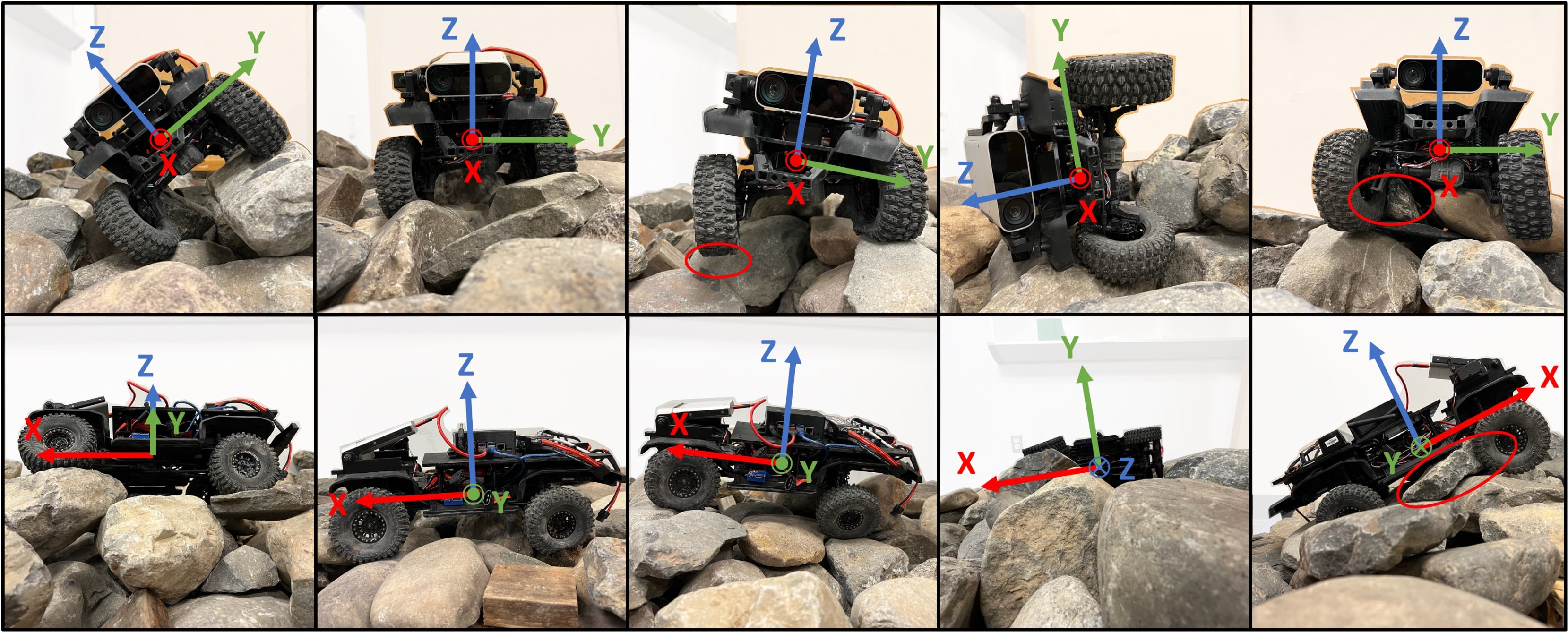
Figure 1: Front and side view (1st and 2nd row) of a wheeled robot navigating vertically challenging terrain: (from left to right) large roll angle, stable chassis, suspended wheel, roll-over, and get-stuck.

In this paper, we develop a learning approach to model 3D vehicle-terrain interactions and plan vehicle trajectories to drive wheeled robots on vertically challenging terrain. Considering the difficulty in analytically modeling and computing vehicle poses using complex vehicle dynamics [22, 23, 24] in real time, we adopt a data-driven approach to model the forward vehicle-terrain dynamics based on terrain elevation maps along potential future trajectories. We develop a Wheeled Mobility on Vertically Challenging Terrain (wm-vct) planner, which uses our learned model’s output in a novel cost function in 3D and produces feasible, stable, and efficient motion plans to autonomously navigate wheeled robots on vertically challenging terrain. We present extensive physical experiment results on two wheeled robot platforms and compare our learning approach against four existing baselines and show that our learned model can achieve up to 60% improvement in navigation success rate and 46% reduction in unstable chassis roll and pitch angles.

II RELATED WORK

We review related work in 2D robot navigation in planar workspaces, facilitating mobility on vertically challenging terrain, and machine learning approaches for mobile robots.

II-A 2D Rigid-Body Navigation in Planar Workspaces

Roboticists have been developing classical ground navigation planners for decades [4, 5, 6]. Recently, researchers have also investigated high-speed [25, 26], off-road [27, 28, 29], and social [30, 31, 32, 33, 34, 35, 36] navigation. In the aforementioned research thrusts, most robots are modeled as 2D rigid bodies (e.g., bounding boxes) and most feasible navigation plans are in 2D and collision-free, regardless of the robot type (e.g., wheeled or tracked). In order to allow wheeled mobile robots to venture into other difficult-to-reach spaces, recent work has extended wheeled mobility to vertically challenging terrain [17], considering that vertical protrusions from the ground are not uncommon in real-world unstructured environments [14, 15]. However, both rigid body and planar workspace assumptions are no longer valid in such spaces, requiring new methods to model the interactions between the non-rigid robots and 3D environments.

II-B Robot Mobility on Vertically Challenging Terrain

Most research aiming at allowing robots to move in vertically challenging environments are from the hardware side. Still treating vehicles as rigid bodies, tracked vehicles are expected to crawl over more rugged terrain than wheeled platforms due to the increased surface contact and therefore propulsion [37], while adhesive materials [13] and tethers [16] allow robots to overcome gravity while climbing vertical slopes. Relaxing the assumption of rigid body, vehicles with active suspensions have been developed [10, 11, 12] to proactively maintain a stable pose of the chassis on vertically challenging terrain. Highly articulated systems, e.g., legged [38, 39], wheel-legged [40, 41], or snake [42, 18] robots, are another choice to negotiate through such terrain with a stable torso, or virtual chassis for limbless snake robots [43], by solving many Degrees-of-Freedom (DoFs) of the robot joints. However, despite the versatility to overcome verticality, such specialized hardware are expensive, inefficient (especially on flat terrain), and not as common as conventional wheeled robots.

II-C Machine Learning for Robot Mobility

In addition to the aforementioned classical methods, roboticists have also started utilizing data-driven approaches for robot mobility [44]. Learning from data, robots no longer need hand-crafted models [26, 45, 46], cost functions [47, 48, 33, 49], or planner parameters [50, 51, 52, 53, 54, 55], see beyond sensor range [56, 57], and acquire navigation behaviors end-to-end from sensor data [58, 59, 60, 61, 62, 63, 64, 65, 66]. Researchers have also used end-to-end Behavior Cloning (BC) [67] to address wheeled mobility on vertically challenging terrain [17]. Considering the power of machine learning and drawbacks of end-to-end BC (e.g., data-hungry, prone to overfitting, and not generalizable), this work takes a structured learning approach to only model the vehicle-terrain forward dynamics, then constructs a novel cost function in 3D specifically tailored for vertically challenging terrain, and finally plans trajectories to move robots toward their goal.

III APPROACH

The difficulties in navigating a wheeled mobile robot on vertically challenging terrain are two fold: (1) the high variability of vehicle poses due to the irregular terrain underneath the robot may overturn the vehicle (rolling-over, 4th column in Fig. 1); (2) not being able to identify that a certain terrain patch is beyond the robot’s mechanical limit and therefore needs to be circumvented may get the robot stuck (immobilization, 5th column in Fig. 1). Therefore, this work takes a structured learning approach to address both challenges by learning a vehicle-terrain forward dynamics model based on the vertically challenging terrain underneath the vehicle, using it to rollout sampled receding-horizon trajectories, and minimizing a cost function to reduce the chance of rolling-over and immobilization and to move the vehicle toward the goal.

III-A Motion Planning Problem Formulation

Consider a discrete vehicle dynamics model of the form $\mathbf{x}_{t+1}=f(\mathbf{x}_{t},\mathbf{u}_{t})$, where $\mathbf{x}_{t}\in X$ and $\mathbf{u}_{t}\in U$ denote the state and input space respectively. In the normal case of 2D navigation planning (Fig. 2 left), $X\subset\mathbb{SE}(2)$ and $X=X_{\textrm{free}}\cup X_{\textrm{obs}}$, where $X_{\textrm{free}}$ and $X_{\textrm{obs}}$ denote free spaces and obstacle regions. $\mathbf{x}_{t}$ includes the translations along the $\mathbf{x}$ and $\mathbf{y}$ axis ($x$ and $y$) and the rotation along the $\mathbf{z}=\mathbf{x}\times\mathbf{y}$ axis (yaw) of a fixed global coordinate system. For input, $\mathbf{u}_{t}=(v_{t},\omega_{t})\in U\subset\mathbb{R}^{2}$, where $v_{t}$ and $\omega_{t}$ are the linear and angular velocity. Finally, let $X_{\textrm{goal}}\subset X$ denote the goal region. The motion planning problem for the conventional 2D navigation case is to find a control function $u:\{t\}_{t=0}^{T-1}\rightarrow U$ that produces an optimal path $\mathbf{x}_{t}\in X_{\textrm{free}},\forall t\in\{t\}_{t=0}^{T}$ from an initial state $\mathbf{x}_{0}=\mathbf{x}_{\textrm{init}}$ to the goal region $\mathbf{x}_{T}\in X_{\textrm{goal}}$ that follows the system dynamics $f(\cdot,\cdot)$ and minimizes a given cost function $c(x)$, which maps from a state trajectory $x:\{t\}_{t=0}^{T}\rightarrow X$ to a positive real number. In many cases, $c(x)$ is simply the total time step $T$ to reach the goal. Considering the difficulty in finding the absolute minimal-cost state trajectory, many mobile robots use sampling-based motion planners to find near-optimal solutions [68, 69].

Conversely, in our case of wheeled mobility on vertically challenging terrain, vehicle state $X\subset\mathbb{SE}(3)$ (i.e., translations and rotations along the $\mathbf{x}$, $\mathbf{y}$, and $\mathbf{z}$ axis) with the same input $\mathbf{u}_{t}=(v_{t},\omega_{t})\in U\subset\mathbb{R}^{2}$. The system dynamics enforces that $\mathbf{x}_{t}$ is always “on top of” a subset of $X_{\textrm{obs}}$ (i.e., vertically challenging terrain underneath and supporting the robot) or some boundary of $X$ (i.e., on a flat ground) due to gravity, requiring a 3D, 6-DoF vehicle-terrain dynamics model in $\mathbb{SE}(3)$ (Fig. 2 right).

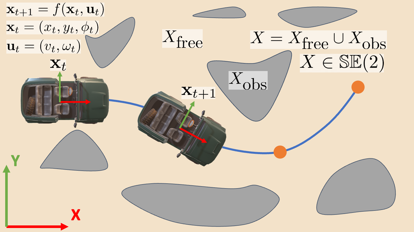
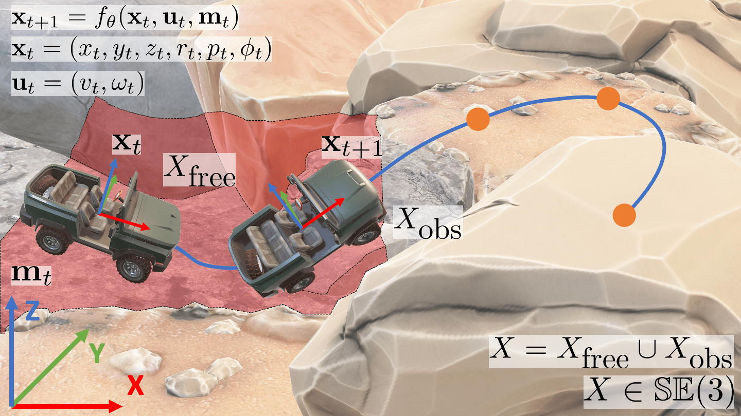
Figure 2: 2D navigation in $\mathbb{SE}(2)$ vs. 3D, 6-DoF navigation on vertically challenging terrain in $\mathbb{SE}(3)$.

III-B Vehicle-Terrain Dynamics Model Learning

Compared to the simple 2D vehicle dynamics in $\mathbb{SE}(2)$, our non-rigid vehicle-terrain dynamics on vertically challenging terrain in $\mathbb{SE}(3)$ becomes more difficult to model, considering the complex interaction between the terrain and chassis via the long suspension travel and deflated tire pressure of off-road vehicles to assure adaptivity and traction (Fig. 1). Therefore, this work adopts a data-driven approach to learn the vehicle-terrain dynamics model, which can be used to rollout trajectories for subsequent planning.

To be specific, $\mathbf{x}_{t}=(x_{t},y_{t},z_{t},r_{t},p_{t},\phi_{t})$, where the first and last three denote the translational ($x$, $y$, $z$) and rotational (roll, pitch, yaw) component respectively along the $\mathbf{x}$, $\mathbf{y}$, and $\mathbf{z}$ axis. Note that unlike most 2D navigation problems in which the next vehicle state $\mathbf{x}_{t+1}$ only relies on the current vehicle state $\mathbf{x}_{t}$ and input $\mathbf{u}_{t}$ alone, our next vehicle state is additionally affected by the vertically challenging terrain underneath and in front of the vehicle in the current time step, denoted as $\mathbf{m}_{t}$. Therefore, the forward dynamics on vertically challenging terrain can be formulated as

$$\mathbf{x}_{t+1}=f_{\theta}(\mathbf{x}_{t},\mathbf{u}_{t},\mathbf{m}_{t}),$$ (1)

which is parameterized by $\theta$ and will be learned in a data-driven manner. Training data of size $N$ can be collected by driving a wheeled robot on different vertically challenging terrain and recording the current and next state, current terrain, and current input: $\mathcal{D}=\{\langle\mathbf{x}_{t},\mathbf{x}_{t+1},\mathbf{m}_{t},\mathbf{u}_{t}\rangle_{t=1}^{N}$}. Then we learn $\theta$ by minimizing a supervised loss function:

$$\theta^{*}=\operatorname*{argmin}_{\theta}\sum_{(\mathbf{x}_{t},\mathbf{x}_{t+1},\mathbf{m}_{t},\mathbf{u}_{t})\in\mathcal{D}}\lVert f_{\theta}(\mathbf{x}_{t},\mathbf{u}_{t},\mathbf{m}_{t})-\mathbf{x}_{t+1}\rVert_{H},$$ (2)

where $||\mathbf{v}||_{H}=\mathbf{v}^{T}H\mathbf{v}$ is the norm induced by a positive definite matrix $H$, used to weigh the learning loss of the different dimensions of the vehicle state $\mathbf{x}_{t}$. The learned vehicle-terrain forward dynamics model $f_{\theta}(\cdot,\cdot,\cdot)$ can then be used to rollout future trajectories for minimal-cost planning.

III-C Sampling-Based Receding-Horizon Planning

We adopt a sampling-based receding-horizon planning paradigm, in which the planner first uniformly samples input sequences up until a short horizon $H$, uses the learned model $f_{\theta}$ to rollout state trajectories, evaluates their cost based on a pre-defined cost function, finds the minimal-cost trajectory, executes the first input, replans, and thus gradually moves the horizon closer to the final goal. In this way, the modeling error can be corrected by frequent replanning. However, an under-actuated wheeled robot, i.e., using $\mathbf{u}_{t}=(v_{t},\omega_{t})\in U\subset\mathbb{R}^{2}$ to actuate $\mathbf{x}_{t}=(x_{t},y_{t},z_{t},r_{t},p_{t},\phi_{t})\in X\subset\mathbb{SE}(3)$ subject to $f_{\theta}$, may easily end up in many terminal states outside of $X_{\textrm{goal}}$, which the vehicle cannot escape and recover from, i.e., rolling over or immobilization (getting stuck) due to excessive roll and pitch angles, irregular terrain geometry, and large height change, e.g., on a large rock. Therefore, while our goal is still to minimize the traversal time $T$ leading to $X_{\textrm{goal}}$, for our receding-horizon planner, we seek to optimize five cost terms on a state trajectory $\mathbf{x}_{0:H}=\{\textbf{x}_{t}\}_{t=0}^{H},\textrm{s.t.},\mathbf{x}_{t+1}=f_{\theta}(\mathbf{x}_{t},\mathbf{u}_{t},\mathbf{m}_{t}),\forall t<H$, which starts at the current time $0$ and ends at the horizon $H$, to avoid these two types of terminal states on vertical challenging terrain and also move the robot towards the goal:

$$\begin{split}c(\mathbf{x}_{0:H})=w_{1}c_{\textrm{rp}}(\mathbf{x}_{0:H})+w_{2}c_{\textrm{tg}}(\mathbf{x}_{0:H})+w_{3}c_{\textrm{hc}}(\mathbf{x}_{0:H})\\ +w_{4}c_{\textrm{mb}}(\mathbf{x}_{0:H})+w_{5}c_{\textrm{est}}(x_{H}),\end{split}$$ (3)

where $c_{\textrm{rp}}(\cdot)$, $c_{\textrm{tg}}(\cdot)$, and $c_{\textrm{hc}}(\cdot)$ denote the cost corresponding to the robot’s (extensive) roll and pitch angle, (irregular) underneath terrain geometry, and (large) terrain height change respectively; $c_{\textrm{mb}}(\cdot)$ is the cost of moving out of the observable map boundary; $c_{\textrm{est}}(\cdot)$ is the estimated cost to reach the final goal region $X_{\textrm{goal}}$ from the state on the horizon $x_{H}$, which can be computed by the Euclidean distance $c_{\textrm{est}}(x_{H})=||x_{H}-x_{G}||_{2}$, where $x_{G}$ is any state inside $X_{\textrm{goal}}$. $w_{1}$ to $w_{5}$ are corresponding weights for the cost terms.

III-D Modeling Rolling-Over and Immobilization

Vehicle roll-over is often associated with large roll and pitch angles, which we therefore seek to minimize along the state trajectory. Note that roll $r_{t}$ and pitch $p_{t}$ are part of the vehicle state $\mathbf{x}_{t}$. Therefore, we design a cost term that considers the absolute values of roll and pitch:

$$c_{\textrm{rp}}(\mathbf{x}_{0:H})=w_{1,1}\sum_{t=0}^{H}|r_{t}|+w_{1,2}\sum_{t=0}^{H}|p_{t}|,$$ (4)

where $w_{1,1}$ and $w_{1,2}$ weigh the effect of the absolute value of roll and pitch.

Similarly, vehicle immobilization often happens when the vehicle state does not change from time to time due to irregular underneath terrain geometry. Therefore, trajectories on which vehicle state significantly changes, especially along the translational dimension $x$ and $y$, are encouraged:

$$c_{\textrm{tg}}(\mathbf{x}_{0:H})=-w_{2,1}\sum_{t=1}^{H}|x_{t}-x_{t-1}|-w_{2,2}\sum_{t=1}^{H}|y_{t}-y_{t-1}|,$$ (5)

where $w_{2,1}$ and $w_{2,2}$ weigh the effect of the displacement along $x$ and $y$ direction.

Furthermore, the vehicle should prefer gentle slope rather than large height change to avoid immobilization, so we encourage small displacement in the $z$ direction along the trajectory:

$$c_{\textrm{hc}}(\mathbf{x}_{0:H})=\sum_{t=1}^{H}|z_{t}-z_{t-1}|.$$ (6)

With the cost function (Equation (3)) and cost terms (Equation (4), (5), and (6)) defined, we can use any motion planner to find the minimal-cost 6-DoF state trajectory $\mathbf{x}_{0:H}$ (see details in Section IV).

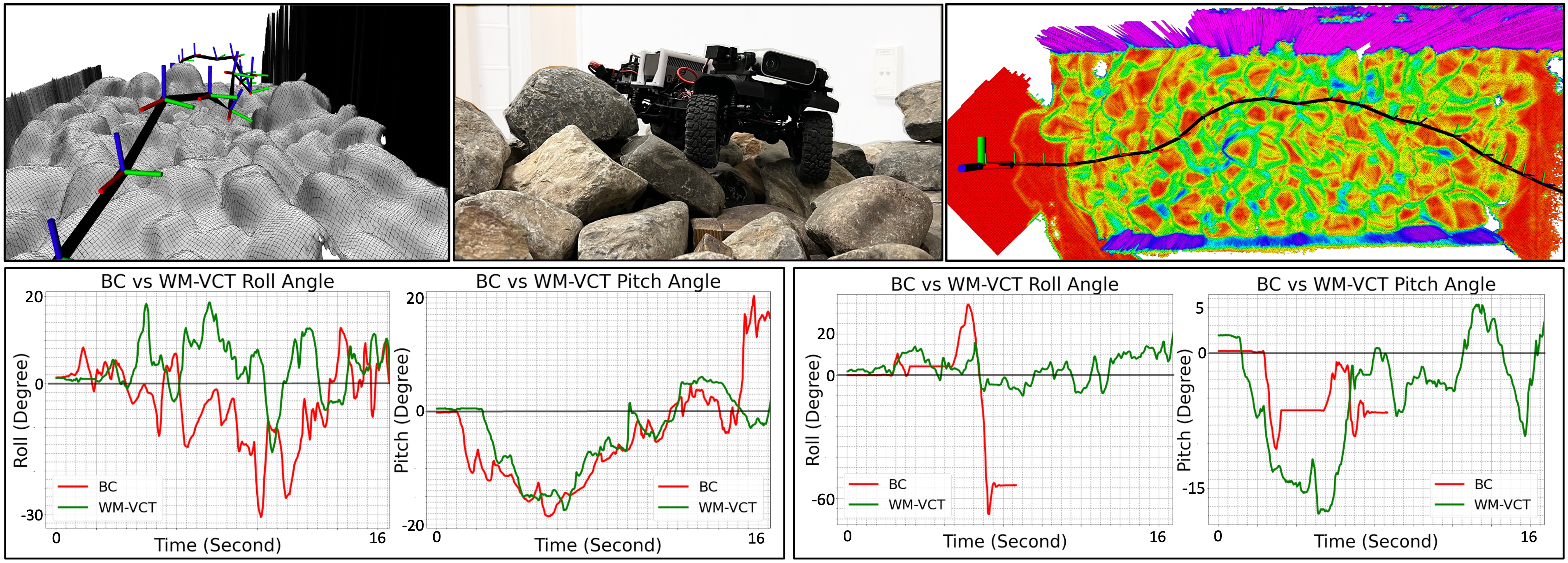
Figure 3: Physical Experiments: The V6W (top middle) navigates through a vertical challenging environment (front and top view of the elevation map shown in top left and top right with the planned 6-DoF vehicle poses and trajectory in black); roll and pitch values of two successful wm-vct trials (green lines at the bottom) are shown, while BC suffers from larger values in the first (red lines bottom left) and fails the second (red lines bottom right).

IV IMPLEMENTATION

We present implementation details of our wm-vct navigation planner onboard two physical wheeled vehicles.

Algorithm 1 wm-vct Planner

1:  Parameters: max iteration $I$ (10), steering sample number $N$ (11), steering range $\Omega_{\textrm{min}}$ and $\Omega_{\textrm{max}}$ ($\pm 0.78\textrm{rad}$), roll-out horizon $H_{\textrm{r}}$ (5), linear velocity $V$ ($0.1\textrm{m/s}$), step size $S$ (1s), update horizon $H_{\textrm{u}}$ (3), and goal_tolerance $G$ (0.02m)

2:  Input: robot pose $P_{\textrm{robot}}$ and goal pose $P_{\textrm{goal}}$

3:  $s_{1}=(x_{1},y_{1},z_{1},r_{1},p_{1},\phi_{1})=P_{\textrm{robot}}$, $T_{\textrm{final}}=\{s_{1}\}$

4:  while max iteration $I$ not reached do

5:     for $\Omega_{i}$ , $i\in[1,N]$, from range $\Omega_{\textrm{min}}$ to $\Omega_{\textrm{max}}$ do

6:        $T_{i}=\{s_{1}\}$

7:        for $t\in[1,H_{\textrm{r}}]$ do

8:           $x_{t+1},y_{t+1},\phi_{t+1}$ = Ackermann($x_{t}$, $y_{t}$, $\phi_{t}$, $V$, $\Omega_{i}$, S)

9:           $z_{t+1}$ = Elevation_Map_Height($x_{t+1}$, $y_{t+1}$)

10:           $\mathbf{m}_{t}$ = Elevation_Map_Patch($x_{t}$, $y_{t}$, $\phi_{t}$, $x_{t+1}$, $y_{t+1}$, $\phi_{t+1}$)

11:           $r_{t+1},p_{t+1}=f_{\theta}(\mathbf{m}_{t},r_{t},p_{t})$ $\triangleright$ learned roll & pitch model

12:           $s_{t+1}=(x_{t+1},y_{t+1},z_{t+1},r_{t+1},p_{t+1},\phi_{t+1})$

13:           $T_{i}.\textrm{add}(s_{t+1})$

14:           if Distance($s_{t+1}$, $P_{\textrm{goal}}$) $\leq$ $G$ then

15:              break $\triangleright$ goal reached, stop rollout

16:           end if

17:        end for

18:        $C_{i}$ = Calculate_Cost($T_{i}$)

19:     end for

20:     $T_{\textrm{best}}=T_{\operatorname*{argmin}_{i}(C_{i})}$ $\triangleright$ minimal-cost traj. up to roll-out horizon

21:     for $s_{j}$ in $T_{\textrm{best}}$, $j\in[1,H_{\textrm{u}}]$  do

22:        $T_{\textrm{final}}.\textrm{add}(s_{j}$) $\triangleright$ backtrack to and add only up till update horizon

23:     end for

24:     if Distance($T_{\textrm{final}}$[last], $P_{\textrm{goal}}$) $\leq$ $G$ then

25:        Return $T_{\textrm{final}}$

26:     end if

27:     $s_{1}=T_{\textrm{final}}$[last] $\triangleright$ update and restart new samples

28:  end while

29:  Return $T_{\textrm{final}}$

IV-A Physical Robots and Vertically Challenging Testbed

We implement our wm-vct planner on two open-source wheeled robot platforms, the Verti-Wheelers (VWs) [17], one with six wheels (V6W, $0.863\textrm{m}\times 0.249\textrm{m}\times 0.2\textrm{m}$) and the other with four wheels (V4W, $0.523\textrm{m}\times 0.249\textrm{m}\times 0.2\textrm{m}$). Both robots are equipped with a Microsoft Azure Kinect RGB-D camera with a 1-DoF gimbal actuated by a servo to fixate the field of view on the terrain in front of the vehicle regardless of chassis pose. NVIDIA Jetson computers (ORIN and Xavier for V6W and V4W respectively) provide onboard computation. We use low-gear and lock both front and rear differentials to improve mobility on vertically challenging terrain. Both robots are tested on a $3.1\textrm{m}\times 1.3\textrm{m}$ rock testbed (with the highest vertical point of $X_{\textrm{obs}}$ reaching 0.6m) composed of hundreds of rocks and boulders of an average size of 30cm, similar to the size of the robots (Fig. 1). The rocks and boulders on the testbed are shuffled many times during experiments. The vehicle state estimation for $\mathbf{x}_{t}$ is provided by an online Visual Inertia Odometry system provided by the rtabmap_ros package [70]. In order to represent $\mathbf{m}_{t}$, we process the RGB-D input into an elevation map [71], a 2D grid where each pixel ($8$mm resolution) indicates the height of the terrain at that point.

IV-B wm-vct Planner Implementation

Our planner implementation is shown in Algorithm 1.

IV-B1 Dynamics Model Decomposition

We decompose the full 6-DoF vehicle-terrain dynamics model $\mathbf{x}_{t+1}=(x_{t+1},y_{t+1},z_{t+1},r_{t+1},p_{t+1},\phi_{t+1})=f_{\theta}(\mathbf{x}_{t},\mathbf{u}_{t},\mathbf{m}_{t})$ into three parts: We utilize a planar Ackermann-steering model to obtain approximate $(x_{t+1},y_{t+1},\phi_{t+1})$ based on $(x_{t},y_{t},\phi_{t})$ and $\mathbf{u}_{t}$ (line 8 in Algorithm 1); $z_{t+1}$ is determined by the value of the elevation map $\mathbf{m}_{t}$ at $(x_{t+1},y_{t+1})$ (line 9); We use a neural network to predict the roll $r_{t+1}$ and pitch $p_{t+1}$ angles based on $\mathbf{m}_{t}$, $r_{t}$, and $p_{t}$ (line 11, potentially with additional history values). In practice, we find such a decomposition very efficient and sufficiently accurate in capturing the 6-DoF vehicle dynamics with a very small amount of training data (approximately 30 minutes) and leave learning the full dynamics model as future work. We use two $40$$\times$$100$ ($0.32$m$\times 0.8$m) elevation maps centered at both the robot’s current and next position and aligned with the current and next yaw angle, i.e., underneath $(x_{t},y_{t})$/$(x_{t+1},y_{t+1})$ and aligned with $\phi_{t}$/$\phi_{t+1}$ (line 10). In our neural network model (Fig. 4), a fully connected sequential head (8000-64-32-8 neurons) processes the $2\times 40\times 100$ elevation maps into a 8-dimensional embedding, which is then concatenated with the 8-dimensional embedding from the last and current roll and pitch angles, $r_{t-1}$, $r_{t}$, $p_{t-1}$, and $p_{t}$, and fed into two more fully connected layers (16-8-2), before finally producing the next roll $r_{t+1}$ and pitch $p_{t+1}$ values. To train the model for each vehicle, we use 43161 data frames for V6W and 41367 for V4W in the open-source Verti-Wheelers datasets [17], roughly 30 minutes of data each demonstrating both VWs crawling over different vertically challenging testbeds.

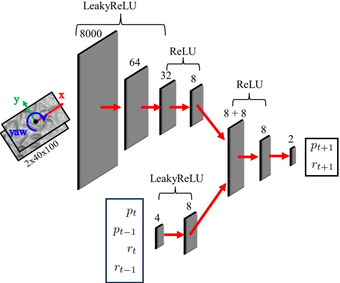
Figure 4: Neural Network Architecture for Roll and Pitch.

IV-B2 Sampling and Roll-Out

For the sampling-based receding-horizon planner, we keep the linear velocity $v$ constant ($0.1\textrm{m/s}$) and sample 11 angular velocities $\omega$, or in our case, steering curvatures evenly from $[-0.78\textrm{rad},0.78\textrm{rad}]$ (line 1). With a step size of 1 second, we roll out our vehicle dynamics model with the 11 $(v,\omega)$ pairs five times (roll-out horizon $H_{\textrm{r}}$, lines 7-17), evaluate the trajectory costs (Equation (3) to (6), line 18) with corresponding cost weights listed in Table I, and expand the search tree again from the 3rd state (update horizon $H_{\textrm{u}}$, lines 21-23) on the lowest-cost trajectory using the same 11 velocity pairs. We repeat this process ten times (max iteration $I$) and find the overall minimal-cost trajectory of horizon 30 ($\mathbf{x}_{0:30}$). Fig. 5 shows the wm-vct sampling and roll-out strategy depicted in Algorithm 1.

TABLE I: Cost Function Weights

$w_{1}$	$w_{2}$	$w_{1,1}$	$w_{1,2}$	$w_{2,1}$	$w_{2,2}$	$w_{3}$	$w_{4}$	$w_{5}$
1	8	0.4	0.4	1	1	0.07	10	4

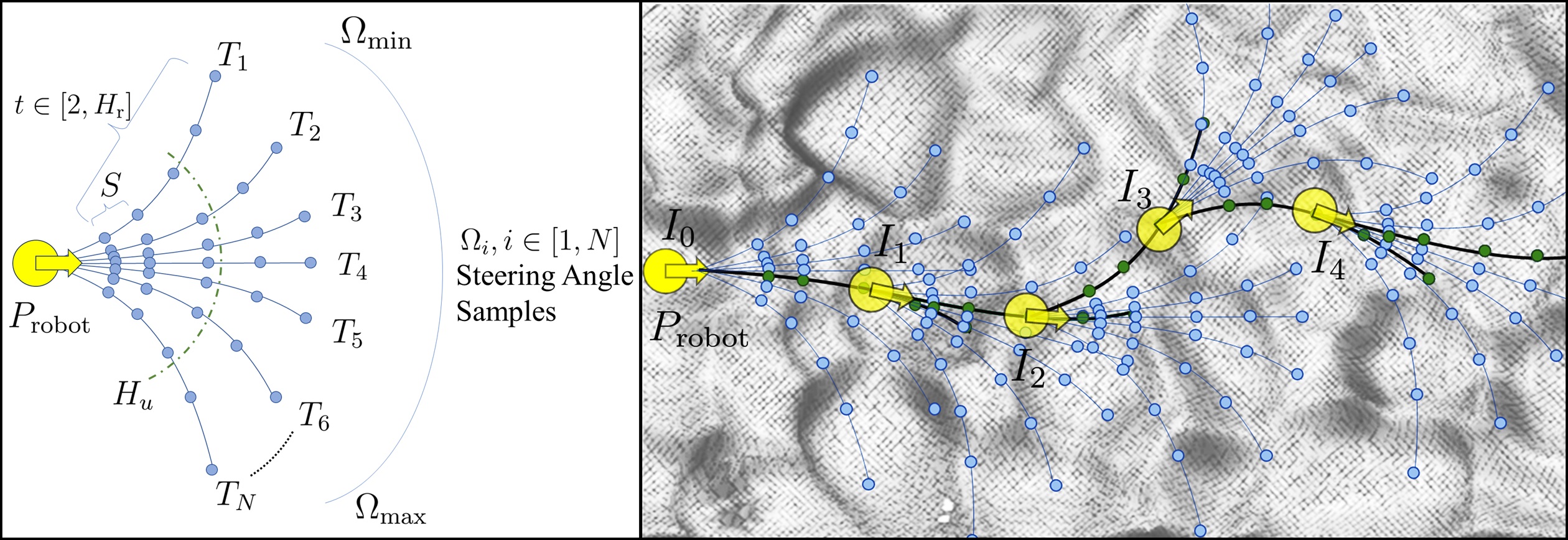
Figure 5: wm-vct Sampling and Roll-Out Strategy.

IV-B3 Motion Controller

We implement a low-level controller operating at a frequency of 30Hz, with the objective of tracking the trajectory that incurs the lowest cost. Specifically, aiming to reach the next state $\mathbf{x}_{t+1}$ from the current state $\mathbf{x}_{t}$, the linear velocity controller determines the throttle command (ranging from $[-1.0,1.0]$) by considering the current pitch angle $p_{t}$: the controller switches throttle command among three intervals, i.e., $0.15$ for pitch less than -5°, 0.20 for pitch from -5° to 5°, and 0.30 for pitch greater than 5°. Such a mechanism approximately maintains constant velocity with respect to changing terrain. The steering angle is calculated by measuring the angle between the current yaw angle $\phi_{t}$ and the line connecting the current 2D position $(x_{t},y_{t})$ to the next position $(x_{t+1},y_{t+1})$. Meanwhile, while the receding-horizon planner constantly replans at 2Hz, the controller will also trigger instant replanning when the distance between the robot and the planned trajectory exceeds a predefined threshold (0.4m).

V EXPERIMENTS

TABLE II: Experiment Results of bc and wm-vct: Number of successful trials (out of 5), mean traversal time (of successful trials in seconds), and average roll/pitch angles (in degrees). ol, rb, and Art fail all trials. Best results are shown in bold.

	V6W		V4W
	bc	wm-vct	bc	wm-vct
Easy	5/5, 15.8s, 7.3°/7.9°	5/5, 24s, 5.1°/7.5°	2/5, 18.0s, 9.2°/17.5°	2/5, 27.5s, 5.8°/9.5°
Medium	3/5, 17.0s, 9.4°/8.3°	4/5, 24.5s, 6.1°/8.6°	1/5, 16.0s, 12°/8.5°	2/5, 32.5s, 7.9°/11.4°
Difficult	1/5, 20.0s, 8.3°/10.7°	4/5, 22.7s, 6.2°/7.4°	N/A	N/A

We provide experiment results and compare wm-vct’s performance against other baselines designed for vertically challenging terrain.

V-A Baselines

Our proposed wm-vct navigation planner is compared against four baselines. The three baseline algorithms developed with the open-source Verti-Wheelers project [17], i.e., Open-Loop (ol), Rule-Based (rb), and Behavior Cloning (bc), are implemented on our robots and compared against wm-vct. We also compare our method against the Art planner [72], a state-of-the-art motion planner based on learned motion cost for quadruped robots to navigate on rough terrain, which is shown to be not applicable for our wheeled vehicle-terrain dynamics. In Fig. 3, we show the V6W navigating the testbed (top middle), front (top left) and top (top right) view of the elevation map with the planned 6-DoF vehicle state trajectory, and pitch and roll values in two example environments (bottom left and right). In the first environment, while both bc (red) and wm-vct (green) succeed, the former experiences larger roll and pitch values; in the second environment, bc (red) fails due to the excessive roll angle around 7.5s, while wm-vct is able to successfully navigate through.

V-B Testbed Experiment Results

We randomly shuffle the testbed three times and test all four baselines against our wm-vct planner. In all our three test environments, neither ol nor rb finish one single trial, either rolling over or getting stuck on challenging rocks. The Art planner aims at planning trajectories that go through flat surfaces for a quadruped to have stable foothold, while the quadruped torso’s roll and pitch angles can be simply stabilized by the many DoFs on the four limbs, which does not apply to wheeled vehicles. It is also designed for a large quadruped robot carrying heavy-duty onboard computation and takes more than 10 seconds for one single planning cycle on the small VWs. Without timely replanning, our controller is not able to follow the outdated trajectory tailored for legged robots and therefore fails every time at difficult scenarios after deviating from the planned path.

We present our experiment results in Table II. The left half shows the V6W results while the right half V4W in the three obstacle courses labeled with three difficulty levels, five trials each. In general, our wm-vct planner achieves better results on both six-wheeled and four-wheeled platforms, compared to bc, the only baseline that can occasionally navigate through, in terms of navigation success rate and average roll and pitch angles. For V6W, both bc and wm-vct finish all five trials in the easy environment, with bc being more aggressive and therefore achieve faster traversal time but larger roll and pitch angles; for the medium difficulty, bc fails two trials due to rolling-over and immobilization, while wm-vct fails only one; in the difficult environment, bc succeeds only one while wm-vct fails only one. Note the shorter traversal time of bc is calculated based on only the successful trials, showing its aggressiveness, while wm-vct has lower roll and pitch angles in most cases (other than slightly larger pitch for Medium). V4W is a much less mechanically capable platform, and therefore fails more than V6W (it fails all trials in the difficult environment with both bc and wm-vct). But the overall comparison between bc and wm-vct remains the same: wm-vct finishes more trials, is slower but more stable, and achieves lower roll and pitch angles overall (except pitch for Medium).

V-C Outdoor Mobility Demonstration

In addition to the controlled testbed experiments, we also deploy wm-vct outdoors in natural vertically challenging terrain with different rock sizes to test our planner’s generalizability. The outdoor environment is unseen in the training set and will challenge bc’s generalizability, while we expect that the limited learning scope of wm-vct can overcome such out-of-distribution scenarios. In fact, wm-vct indeed allows both V6W and V4W to avoid excessive roll and pitch angles and getting stuck on large, unseen rocks in the outdoor environment. As shown in Figure 6, bc fails because the learned end-to-end policy causes excessive roll angle and leads to roll-over (left), while wm-vct’s dynamic model successfully generalizes to the unseen outdoor environment.

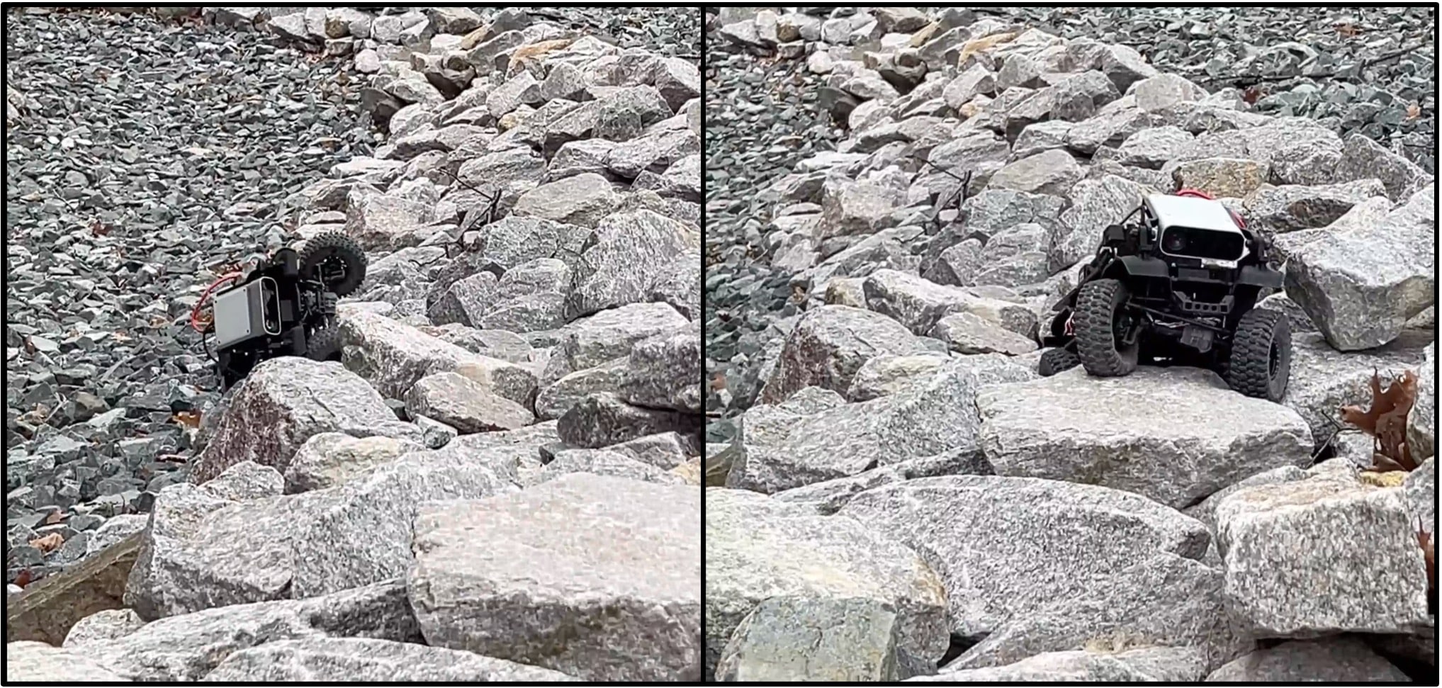
Figure 6: Outdoor Mobility Demonstration: bc rolls over (left) and wm-vct succeeds (right).

VI CONCLUSIONS

We present a learning approach to enable wheeled mobility on vertically challenging terrain. Going beyond the current 2D motion planning assumptions of rigid vehicle bodies and 2D planar workspaces which can be divided into free spaces and obstacles, our wm-vct planner first learns to model the non-rigid vehicle-terrain forward dynamics in $\mathbb{SE}(3)$ based on the current vehicle state, input, and underlying terrain. Leveraging the trajectory roll-outs under a sampling-based receding-horizon planning paradigm using the learned vehicle-terrain forward dynamics, wm-vct constructs a novel cost function in 3D to prevent the vehicle from rolling-over and immobilization when facing previously non-traversable obstacles. We show that our wm-vct planner can produce feasible, stable, and efficient motion plans to drive robots over vertically challenging terrain toward their goal and outperform several state-of-the-art baselines on two physical wheeled robot platforms.

References

- [1] IEEE Spectrum, “Kiva systems – three engineers, hundreds of robots, one warehouse,” https://spectrum.ieee.org/three-engineers-hundreds-of-robots-one-warehouse, 2008, accessed: 2023-05-16.
- [2] iRobot, “iRobot – robot vacuum and mop,” https://www.irobot.com/, 2023, accessed: 2023-05-16.
- [3] Amazon, “Meet scout,” https://www.aboutamazon.com/news/transportation/meet-scout, 2023, accessed: 2023-05-16.
- [4] D. Fox, W. Burgard, and S. Thrun, “The dynamic window approach to collision avoidance,” IEEE Robotics & Automation Magazine, vol. 4, no. 1, pp. 23–33, 1997.
- [5] S. Quinlan and O. Khatib, “Elastic bands: Connecting path planning and control,” in [1993] Proceedings IEEE International Conference on Robotics and Automation. IEEE, 1993, pp. 802–807.
- [6] C. Rösmann, F. Hoffmann, and T. Bertram, “Kinodynamic trajectory optimization and control for car-like robots,” in 2017 IEEE/RSJ International Conference on Intelligent Robots and Systems (IROS). IEEE, 2017, pp. 5681–5686.
- [7] X. Xiao, Z. Xu, Z. Wang, Y. Song, G. Warnell, P. Stone, T. Zhang, S. Ravi, G. Wang, H. Karnan et al., “Autonomous ground navigation in highly constrained spaces: Lessons learned from the benchmark autonomous robot navigation challenge at icra 2022 [competitions],” IEEE Robotics & Automation Magazine, vol. 29, no. 4, pp. 148–156, 2022.
- [8] D. Perille, A. Truong, X. Xiao, and P. Stone, “Benchmarking metric ground navigation,” in 2020 IEEE International Symposium on Safety, Security, and Rescue Robotics (SSRR). IEEE, 2020, pp. 116–121.
- [9] A. Nair, F. Jiang, K. Hou, Z. Xu, S. Li, X. Xiao, and P. Stone, “Dynabarn: Benchmarking metric ground navigation in dynamic environments,” in 2022 IEEE International Symposium on Safety, Security, and Rescue Robotics (SSRR). IEEE, 2022, pp. 347–352.
- [10] F. Cordes, C. Oekermann, A. Babu, D. Kuehn, T. Stark, F. Kirchner, and D. Bremen, “An active suspension system for a planetary rover,” in Proceedings of the International Symposium on Artificial Intelligence, Robotics and Automation in Space (i-SAIRAS), 2014, pp. 17–19.
- [11] M. R. Islam, F. H. Chowdhury, S. Rezwan, M. J. Ishaque, J. U. Akanda, A. S. Tuhel, and B. B. Riddhe, “Novel design and performance analysis of a mars exploration robot: Mars rover mongol pothik,” in 2017 Third International Conference on Research in Computational Intelligence and Communication Networks (ICRCICN). IEEE, 2017, pp. 132–136.
- [12] H. Jiang, G. Xu, W. Zeng, F. Gao, and K. Chong, “Lateral stability of a mobile robot utilizing an active adjustable suspension,” Applied Sciences, vol. 9, no. 20, p. 4410, 2019.
- [13] Y. Liu and T. Seo, “Anyclimb-ii: Dry-adhesive linkage-type climbing robot for uneven vertical surfaces,” Mechanism and Machine Theory, vol. 124, pp. 197–210, 2018.
- [14] R. R. Murphy, Disaster robotics. MIT press, 2014.
- [15] X. Xiao and R. Murphy, “A review on snake robot testbeds in granular and restricted maneuverability spaces,” Robotics and Autonomous Systems, vol. 110, pp. 160–172, 2018.
- [16] P. McGarey, F. Pomerleau, and T. D. Barfoot, “System design of a tethered robotic explorer (trex) for 3d mapping of steep terrain and harsh environments,” in Field and Service Robotics: Results of the 10th International Conference. Springer, 2016, pp. 267–281.
- [17] A. Datar, C. Pan, M. Nazeri, and X. Xiao, “Toward wheeled mobility on vertically challenging terrain: Platforms, datasets, and algorithms,” arXiv preprint arXiv:2303.00998, 2023.
- [18] X. Xiao, E. Cappo, W. Zhen, J. Dai, K. Sun, C. Gong, M. J. Travers, and H. Choset, “Locomotive reduction for snake robots,” in 2015 IEEE International Conference on Robotics and Automation (ICRA). IEEE, 2015, pp. 3735–3740.
- [19] R. Murphy, J. Dufek, T. Sarmiento, G. Wilde, X. Xiao, J. Braun, L. Mullen, R. Smith, S. Allred, J. Adams et al., “Two case studies and gaps analysis of flood assessment for emergency management with small unmanned aerial systems,” in 2016 IEEE international symposium on safety, security, and rescue robotics (SSRR). IEEE, 2016, pp. 54–61.
- [20] X. Xiao, J. Dufek, T. Woodbury, and R. Murphy, “Uav assisted usv visual navigation for marine mass casualty incident response,” in 2017 IEEE/RSJ International Conference on Intelligent Robots and Systems (IROS). IEEE, 2017, pp. 6105–6110.
- [21] X. Xiao, J. Dufek, and R. R. Murphy, “Autonomous visual assistance for robot operations using a tethered uav,” in Field and Service Robotics: Results of the 12th International Conference. Springer, 2021, pp. 15–29.
- [22] R. N. Jazar, Vehicle dynamics. Springer, 2008, vol. 1.
- [23] G. Yan, M. Fang, and J. Xu, “Analysis and experiment of time-delayed optimal control for vehicle suspension system,” Journal of Sound and Vibration, vol. 446, pp. 144–158, 2019.
- [24] A. A. Aly and F. A. Salem, “Vehicle suspension systems control: a review,” International journal of control, automation and systems, vol. 2, no. 2, pp. 46–54, 2013.
- [25] P. Atreya, H. Karnan, K. S. Sikand, X. Xiao, S. Rabiee, and J. Biswas, “High-speed accurate robot control using learned forward kinodynamics and non-linear least squares optimization,” in 2022 IEEE/RSJ International Conference on Intelligent Robots and Systems (IROS). IEEE, 2022, pp. 11 789–11 795.
- [26] X. Xiao, J. Biswas, and P. Stone, “Learning inverse kinodynamics for accurate high-speed off-road navigation on unstructured terrain,” IEEE Robotics and Automation Letters, vol. 6, no. 3, pp. 6054–6060, 2021.
- [27] R. Manduchi, A. Castano, A. Talukder, and L. Matthies, “Obstacle detection and terrain classification for autonomous off-road navigation,” Autonomous robots, vol. 18, pp. 81–102, 2005.
- [28] L. D. Jackel, E. Krotkov, M. Perschbacher, J. Pippine, and C. Sullivan, “The darpa lagr program: Goals, challenges, methodology, and phase i results,” Journal of Field robotics, vol. 23, no. 11-12, pp. 945–973, 2006.
- [29] H. Mousazadeh, “A technical review on navigation systems of agricultural autonomous off-road vehicles,” Journal of Terramechanics, vol. 50, no. 3, pp. 211–232, 2013.
- [30] R. Mirsky, X. Xiao, J. Hart, and P. Stone, “Conflict avoidance in social navigation–a survey,” arXiv preprint arXiv:2106.12113, 2021.
- [31] H. Karnan, A. Nair, X. Xiao, G. Warnell, S. Pirk, A. Toshev, J. Hart, J. Biswas, and P. Stone, “Socially compliant navigation dataset (scand): A large-scale dataset of demonstrations for social navigation,” IEEE Robotics and Automation Letters, vol. 7, no. 4, pp. 11 807–11 814, 2022.
- [32] Y. F. Chen, M. Everett, M. Liu, and J. P. How, “Socially aware motion planning with deep reinforcement learning,” in 2017 IEEE/RSJ International Conference on Intelligent Robots and Systems (IROS). IEEE, 2017, pp. 1343–1350.
- [33] X. Xiao, T. Zhang, K. M. Choromanski, T.-W. E. Lee, A. Francis, J. Varley, S. Tu, S. Singh, P. Xu, F. Xia, S. M. Persson, L. Takayama, R. Frostig, J. Tan, C. Parada, and V. Sindhwani, “Learning model predictive controllers with real-time attention for real-world navigation,” in Conference on robot learning. PMLR, 2022.
- [34] A. Francis, C. Pérez-d’Arpino, C. Li, F. Xia, A. Alahi, R. Alami, A. Bera, A. Biswas, J. Biswas, R. Chandra et al., “Principles and guidelines for evaluating social robot navigation algorithms,” arXiv preprint arXiv:2306.16740, 2023.
- [35] J.-S. Park, X. Xiao, G. Warnell, H. Yedidsion, and P. Stone, “Learning perceptual hallucination for multi-robot navigation in narrow hallways,” in 2023 IEEE International Conference on Robotics and Automation (ICRA). IEEE, 2023, pp. 10 033–10 039.
- [36] D. M. Nguyen, M. Nazeri, A. Payandeh, A. Datar, and X. Xiao, “Toward human-like social robot navigation: A large-scale, multi-modal, social human navigation dataset,” in 2023 IEEE/RSJ International Conference on Intelligent Robots and Systems (IROS). IEEE, 2023.
- [37] Q.-H. Vu, B.-S. Kim, and J.-B. Song, “Autonomous stair climbing algorithm for a small four-tracked robot,” in 2008 International Conference on Control, Automation and Systems. IEEE, 2008, pp. 2356–2360.
- [38] P. Fankhauser, M. Bloesch, and M. Hutter, “Probabilistic terrain mapping for mobile robots with uncertain localization,” IEEE Robotics and Automation Letters (RA-L), vol. 3, no. 4, pp. 3019–3026, 2018.
- [39] A. Kumar, Z. Fu, D. Pathak, and J. Malik, “Rma: Rapid motor adaptation for legged robots,” in Robotics: Science and Systems, 2021.
- [40] C. Zheng, S. Sane, K. Lee, V. Kalyanram, and K. Lee, “-waltr: Adaptive wheel-and-leg transformable robot for versatile multiterrain locomotion,” IEEE Transactions on Robotics, 2022.
- [41] K. Xu, Y. Lu, L. Shi, J. Li, S. Wang, and T. Lei, “Whole-body stability control with high contact redundancy for wheel-legged hexapod robot driving over rough terrain,” Mechanism and Machine Theory, vol. 181, p. 105199, 2023.
- [42] C. Wright, A. Johnson, A. Peck, Z. McCord, A. Naaktgeboren, P. Gianfortoni, M. Gonzalez-Rivero, R. Hatton, and H. Choset, “Design of a modular snake robot,” in 2007 IEEE/RSJ International Conference on Intelligent Robots and Systems. IEEE, 2007, pp. 2609–2614.
- [43] D. Rollinson and H. Choset, “Virtual chassis for snake robots,” in 2011 IEEE/RSJ International Conference on Intelligent Robots and Systems. IEEE, 2011, pp. 221–226.
- [44] X. Xiao, B. Liu, G. Warnell, and P. Stone, “Motion planning and control for mobile robot navigation using machine learning: a survey,” Autonomous Robots, vol. 46, no. 5, pp. 569–597, 2022.
- [45] M. Sivaprakasam, S. Triest, W. Wang, P. Yin, and S. Scherer, “Improving off-road planning techniques with learned costs from physical interactions,” in 2021 IEEE International Conference on Robotics and Automation (ICRA). IEEE, 2021, pp. 4844–4850.
- [46] H. Karnan, K. S. Sikand, P. Atreya, S. Rabiee, X. Xiao, G. Warnell, P. Stone, and J. Biswas, “Vi-ikd: High-speed accurate off-road navigation using learned visual-inertial inverse kinodynamics,” in 2022 IEEE/RSJ International Conference on Intelligent Robots and Systems (IROS). IEEE, 2022, pp. 3294–3301.
- [47] D. Vasquez, B. Okal, and K. O. Arras, “Inverse reinforcement learning algorithms and features for robot navigation in crowds: an experimental comparison,” in 2014 IEEE/RSJ International Conference on Intelligent Robots and Systems. IEEE, 2014, pp. 1341–1346.
- [48] M. Wigness, J. G. Rogers, and L. E. Navarro-Serment, “Robot navigation from human demonstration: Learning control behaviors,” in 2018 IEEE International Conference on Robotics and Automation (ICRA). IEEE, 2018, pp. 1150–1157.
- [49] K. S. Sikand, S. Rabiee, A. Uccello, X. Xiao, G. Warnell, and J. Biswas, “Visual representation learning for preference-aware path planning,” in 2022 International Conference on Robotics and Automation (ICRA). IEEE, 2022, pp. 11 303–11 309.
- [50] X. Xiao, B. Liu, G. Warnell, J. Fink, and P. Stone, “Appld: Adaptive planner parameter learning from demonstration,” IEEE Robotics and Automation Letters, vol. 5, no. 3, pp. 4541–4547, 2020.
- [51] Z. Wang, X. Xiao, B. Liu, G. Warnell, and P. Stone, “Appli: Adaptive planner parameter learning from interventions,” in 2021 IEEE international conference on robotics and automation (ICRA). IEEE, 2021, pp. 6079–6085.
- [52] Z. Wang, X. Xiao, G. Warnell, and P. Stone, “Apple: Adaptive planner parameter learning from evaluative feedback,” IEEE Robotics and Automation Letters, vol. 6, no. 4, pp. 7744–7749, 2021.
- [53] Z. Xu, G. Dhamankar, A. Nair, X. Xiao, G. Warnell, B. Liu, Z. Wang, and P. Stone, “Applr: Adaptive planner parameter learning from reinforcement,” in 2021 IEEE international conference on robotics and automation (ICRA). IEEE, 2021, pp. 6086–6092.
- [54] X. Xiao, Z. Wang, Z. Xu, B. Liu, G. Warnell, G. Dhamankar, A. Nair, and P. Stone, “Appl: Adaptive planner parameter learning,” Robotics and Autonomous Systems, vol. 154, p. 104132, 2022.
- [55] Z. Xu, X. Xiao, G. Warnell, A. Nair, and P. Stone, “Machine learning methods for local motion planning: A study of end-to-end vs. parameter learning,” in 2021 IEEE International Symposium on Safety, Security, and Rescue Robotics (SSRR). IEEE, 2021, pp. 217–222.
- [56] M. Everett, J. Miller, and J. P. How, “Planning beyond the sensing horizon using a learned context,” in 2019 IEEE/RSJ International Conference on Intelligent Robots and Systems (IROS). IEEE, 2019, pp. 1064–1071.
- [57] X. Meng, N. Hatch, A. Lambert, A. Li, N. Wagener, M. Schmittle, J. Lee, W. Yuan, Z. Chen, S. Deng et al., “Terrainnet: Visual modeling of complex terrain for high-speed, off-road navigation,” arXiv preprint arXiv:2303.15771, 2023.
- [58] Y. Pan, C.-A. Cheng, K. Saigol, K. Lee, X. Yan, E. A. Theodorou, and B. Boots, “Imitation learning for agile autonomous driving,” The International Journal of Robotics Research, vol. 39, no. 2-3, pp. 286–302, 2020.
- [59] A. Faust, K. Oslund, O. Ramirez, A. Francis, L. Tapia, M. Fiser, and J. Davidson, “Prm-rl: Long-range robotic navigation tasks by combining reinforcement learning and sampling-based planning,” in 2018 IEEE International Conference on Robotics and Automation (ICRA). IEEE, 2018, pp. 5113–5120.
- [60] M. Pfeiffer, M. Schaeuble, J. Nieto, R. Siegwart, and C. Cadena, “From perception to decision: A data-driven approach to end-to-end motion planning for autonomous ground robots,” in IEEE International Conference on Robotics and Automation. IEEE, 2017.
- [61] X. Xiao, B. Liu, G. Warnell, and P. Stone, “Toward agile maneuvers in highly constrained spaces: Learning from hallucination,” IEEE Robotics and Automation Letters, vol. 6, no. 2, pp. 1503–1510, 2021.
- [62] X. Xiao, B. Liu, and P. Stone, “Agile robot navigation through hallucinated learning and sober deployment,” in 2021 IEEE international conference on robotics and automation (ICRA). IEEE, 2021, pp. 7316–7322.
- [63] Z. Wang, X. Xiao, A. J. Nettekoven, K. Umasankar, A. Singh, S. Bommakanti, U. Topcu, and P. Stone, “From agile ground to aerial navigation: Learning from learned hallucination,” in 2021 IEEE/RSJ International Conference on Intelligent Robots and Systems (IROS). IEEE, 2021, pp. 148–153.
- [64] B. Liu, X. Xiao, and P. Stone, “A lifelong learning approach to mobile robot navigation,” IEEE Robotics and Automation Letters, vol. 6, no. 2, pp. 1090–1096, 2021.
- [65] Z. Xu, B. Liu, X. Xiao, A. Nair, and P. Stone, “Benchmarking reinforcement learning techniques for autonomous navigation,” in 2023 IEEE International Conference on Robotics and Automation (ICRA). IEEE, 2023, pp. 9224–9230.
- [66] H. Karnan, G. Warnell, X. Xiao, and P. Stone, “Voila: Visual-observation-only imitation learning for autonomous navigation,” in 2022 International Conference on Robotics and Automation (ICRA). IEEE, 2022, pp. 2497–2503.
- [67] M. Bojarski, D. Del Testa, D. Dworakowski, B. Firner, B. Flepp, P. Goyal, L. D. Jackel, M. Monfort, U. Muller, J. Zhang et al., “End to end learning for self-driving cars,” arXiv preprint arXiv:1604.07316, 2016.
- [68] S. Karaman and E. Frazzoli, “Incremental sampling-based algorithms for optimal motion planning,” Robotics Science and Systems VI, vol. 104, no. 2, 2010.
- [69] S. Karaman, M. R. Walter, A. Perez, E. Frazzoli, and S. Teller, “Anytime motion planning using the rrt,” in 2011 IEEE international conference on robotics and automation. IEEE, 2011, pp. 1478–1483.
- [70] ROS, “rtabmap_ros - ros wiki,” http://wiki.ros.org/rtabmap_ros, 2023, accessed: 2023-06-07.
- [71] T. Miki, L. Wellhausen, R. Grandia, F. Jenelten, T. Homberger, and M. Hutter, “Elevation mapping for locomotion and navigation using gpu,” 2022.
- [72] L. Wellhausen and M. Hutter, “Artplanner: Robust legged robot navigation in the field,” in Field Robotics, 2023.