Multi-type critical process: a birth-death model of error catastrophe

Abstract.

Critical birth-death processes with $n$ distinct types are investigated. Each type $i$ cell divides independently $(i)\to(i)+(i)$ or mutates $(i)\to(i+1)$ at the same rate. The total number of cells grows exponentially as a Yule process until the maximal type $n$ cells appear, which cannot mutate but die at rate one. The last type makes the process critical and hence after the exponentially growing phase eventually all cells die with probability one. The process mimics the accumulation of mutations in a growing population where too many mutations are lethal. This has applications for understanding the mutational burden and so-called error catastrophe in cancer, bacteria, or virus. We present large-time asymptotic results for the general $n$-type critical birth-death process. We find that the mass function of the number of cells of type $k$ has algebraic and stationary tail $(\text{size})^{-1-\chi_{k}}$, with $\chi_{k}=2^{1-k}$, for $k=2,\dots,n$, in sharp contrast to the exponential tail of the first type. The same exponents describe the tail of the asymptotic survival probability $(\text{time})^{-\chi_{n}}$. We discuss the consequences and applications of the results for studying extinction due to mutational burden in biological populations.

1. Introduction

Continuous-time multi-type birth-death processes have been extensively investigated and applied to studying biological populations, providing valuable insight into the evolutionary dynamics of bacteria and cancer growth [12, 39, 22]. Due to their applicability to model exponentially growing populations, a large number of solutions have been derived for multi-type super-critical processes [13, 24]. In this work, we propose asymptotic solutions for the multi-type critical process, where all types of cells have balanced birth and death rates. We show that the multi-type critical process with a finite number of types naturally models the interesting behaviour of populations that grow exponentially but eventually go extinct due genetic instability. This behaviour cannot be captured by the generic super-critical and sub-critical processes and underlies important phenomena including the extinction of tumours and bacterial populations due to mutational burden [31, 28].

Consider the simplest multi-type critical process, each type-$i$ cell divides independently $(i)\to(i)+(i)$ at rate one, or mutates $(i)\to(i+1)$ also at rate one. We additionally assume that $n$ alterations are too much for a cell to bear, hence type $n$ cells die at rate 1. We represent this birth-mutation process by the following scheme

(1) $$\begin{split}\lx@xy@svg{\hbox{\raise 0.0pt\hbox{\kern 21.88889pt\hbox{\ignorespaces\ignorespaces\ignorespaces\hbox{\vtop{\kern 0.0pt\offinterlineskip\halign{\entry@#!@&&\entry@@#!@\cr&&&&\\&&&&\crcr}}}\ignorespaces{\hbox{\kern-21.88889pt\raise 0.0pt\hbox{\hbox{\kern 0.0pt\raise 0.0pt\hbox{\hbox{\kern 3.0pt\raise 0.0pt\hbox{$\textstyle{(1)+(1)}$}}}}}}}{\hbox{\kern 45.88889pt\raise 0.0pt\hbox{\hbox{\kern 0.0pt\raise 0.0pt\hbox{\hbox{\kern 3.0pt\raise 0.0pt\hbox{$\textstyle{(2)+(2)}$}}}}}}}{\hbox{\kern 117.41666pt\raise 0.0pt\hbox{\hbox{\kern 0.0pt\raise 0.0pt\hbox{\hbox{\kern 3.0pt\raise 0.0pt\hbox{$\textstyle{}$}}}}}}}{\hbox{\kern 151.16666pt\raise 0.0pt\hbox{\hbox{\kern 0.0pt\raise 0.0pt\hbox{\hbox{\kern 3.0pt\raise 0.0pt\hbox{$\textstyle{(n)+(n)}$}}}}}}}{\hbox{\kern 223.4491pt\raise 0.0pt\hbox{\hbox{\kern 0.0pt\raise 0.0pt\hbox{\hbox{\kern 3.0pt\raise 0.0pt\hbox{$\textstyle{}$}}}}}}}{\hbox{\kern-9.3889pt\raise-40.0pt\hbox{\hbox{\kern 0.0pt\raise 0.0pt\hbox{\hbox{\kern 3.0pt\raise 0.0pt\hbox{$\textstyle{(1)\ignorespaces\ignorespaces\ignorespaces\ignorespaces\ignorespaces\ignorespaces\ignorespaces\ignorespaces}$}}}}}}}\ignorespaces\ignorespaces\ignorespaces\ignorespaces{}{\hbox{\lx@xy@droprule}}\ignorespaces{\hbox{\kern 0.0pt\raise-5.5pt\hbox{\hbox{\kern 0.0pt\raise 0.0pt\hbox{\lx@xy@tip{1}\lx@xy@tip{-1}}}}}}{\hbox{\lx@xy@droprule}}{\hbox{\lx@xy@droprule}}\ignorespaces\ignorespaces\ignorespaces\ignorespaces{}{\hbox{\lx@xy@droprule}}\ignorespaces{\hbox{\kern 58.38887pt\raise-40.0pt\hbox{\hbox{\kern 0.0pt\raise 0.0pt\hbox{\lx@xy@tip{1}\lx@xy@tip{-1}}}}}}{\hbox{\lx@xy@droprule}}{\hbox{\lx@xy@droprule}}{\hbox{\kern 58.38887pt\raise-40.0pt\hbox{\hbox{\kern 0.0pt\raise 0.0pt\hbox{\hbox{\kern 3.0pt\raise 0.0pt\hbox{$\textstyle{(2)\ignorespaces\ignorespaces\ignorespaces\ignorespaces\ignorespaces\ignorespaces\ignorespaces\ignorespaces}$}}}}}}}\ignorespaces\ignorespaces\ignorespaces\ignorespaces{}{\hbox{\lx@xy@droprule}}\ignorespaces{\hbox{\kern 67.77777pt\raise-5.5pt\hbox{\hbox{\kern 0.0pt\raise 0.0pt\hbox{\lx@xy@tip{1}\lx@xy@tip{-1}}}}}}{\hbox{\lx@xy@droprule}}{\hbox{\lx@xy@droprule}}\ignorespaces\ignorespaces\ignorespaces\ignorespaces{}{\hbox{\lx@xy@droprule}}\ignorespaces{\hbox{\kern 113.66666pt\raise-40.0pt\hbox{\hbox{\kern 0.0pt\raise 0.0pt\hbox{\lx@xy@tip{1}\lx@xy@tip{-1}}}}}}{\hbox{\lx@xy@droprule}}{\hbox{\lx@xy@droprule}}{\hbox{\kern 113.66666pt\raise-40.0pt\hbox{\hbox{\kern 0.0pt\raise 0.0pt\hbox{\hbox{\kern 3.0pt\raise 0.0pt\hbox{$\textstyle{\cdots\ignorespaces\ignorespaces\ignorespaces\ignorespaces}$}}}}}}}\ignorespaces\ignorespaces\ignorespaces\ignorespaces{}{\hbox{\lx@xy@droprule}}\ignorespaces{\hbox{\kern 164.1678pt\raise-40.0pt\hbox{\hbox{\kern 0.0pt\raise 0.0pt\hbox{\lx@xy@tip{1}\lx@xy@tip{-1}}}}}}{\hbox{\lx@xy@droprule}}{\hbox{\lx@xy@droprule}}{\hbox{\kern 164.1678pt\raise-40.0pt\hbox{\hbox{\kern 0.0pt\raise 0.0pt\hbox{\hbox{\kern 3.0pt\raise 0.0pt\hbox{$\textstyle{(n)\ignorespaces\ignorespaces\ignorespaces\ignorespaces\ignorespaces\ignorespaces\ignorespaces\ignorespaces}$}}}}}}}\ignorespaces\ignorespaces\ignorespaces\ignorespaces{}{\hbox{\lx@xy@droprule}}\ignorespaces{\hbox{\kern 174.05788pt\raise-5.5pt\hbox{\hbox{\kern 0.0pt\raise 0.0pt\hbox{\lx@xy@tip{1}\lx@xy@tip{-1}}}}}}{\hbox{\lx@xy@droprule}}{\hbox{\lx@xy@droprule}}\ignorespaces\ignorespaces\ignorespaces\ignorespaces{}{\hbox{\lx@xy@droprule}}\ignorespaces{\hbox{\kern 220.9491pt\raise-40.0pt\hbox{\hbox{\kern 0.0pt\raise 0.0pt\hbox{\lx@xy@tip{1}\lx@xy@tip{-1}}}}}}{\hbox{\lx@xy@droprule}}{\hbox{\lx@xy@droprule}}{\hbox{\kern 220.9491pt\raise-40.0pt\hbox{\hbox{\kern 0.0pt\raise 0.0pt\hbox{\hbox{\kern 3.0pt\raise 0.0pt\hbox{$\textstyle{\emptyset}$}}}}}}}\ignorespaces}}}}\ignorespaces\end{split} \textstyle{(1)+(1)} \textstyle{(2)+(2)} \textstyle{(n)+(n)} \textstyle{(1)\ignorespaces\ignorespaces\ignorespaces\ignorespaces\ignorespaces\ignorespaces\ignorespaces\ignorespaces} \textstyle{(2)\ignorespaces\ignorespaces\ignorespaces\ignorespaces\ignorespaces\ignorespaces\ignorespaces\ignorespaces} \textstyle{\cdots\ignorespaces\ignorespaces\ignorespaces\ignorespaces} \textstyle{(n)\ignorespaces\ignorespaces\ignorespaces\ignorespaces\ignorespaces\ignorespaces\ignorespaces\ignorespaces} \textstyle{\emptyset} \textstyle{(1)+(1)} \textstyle{(2)+(2)} \textstyle{(n)+(n)} \textstyle{(1)\ignorespaces\ignorespaces\ignorespaces\ignorespaces\ignorespaces\ignorespaces\ignorespaces\ignorespaces} \textstyle{(2)\ignorespaces\ignorespaces\ignorespaces\ignorespaces\ignorespaces\ignorespaces\ignorespaces\ignorespaces} \textstyle{\cdots\ignorespaces\ignorespaces\ignorespaces\ignorespaces} \textstyle{(n)\ignorespaces\ignorespaces\ignorespaces\ignorespaces\ignorespaces\ignorespaces\ignorespaces\ignorespaces} \textstyle{\emptyset}$$

A more general and biologically relevant version comes from introducing death and allowing different types of cells to divide and mutate at different rates. We refer to this as the $n$-type birth-death process, which can be illustrated as

(2) $$\begin{split}\lx@xy@svg{\hbox{\raise 0.0pt\hbox{\kern 21.88889pt\hbox{\ignorespaces\ignorespaces\ignorespaces\hbox{\vtop{\kern 0.0pt\offinterlineskip\halign{\entry@#!@&&\entry@@#!@\cr&&&\\&&&\\&&&\crcr}}}\ignorespaces{\hbox{\kern-21.88889pt\raise 0.0pt\hbox{\hbox{\kern 0.0pt\raise 0.0pt\hbox{\hbox{\kern 3.0pt\raise 0.0pt\hbox{$\textstyle{(1)+(1)}$}}}}}}}{\hbox{\kern 45.88889pt\raise 0.0pt\hbox{\hbox{\kern 0.0pt\raise 0.0pt\hbox{\hbox{\kern 3.0pt\raise 0.0pt\hbox{$\textstyle{(2)+(2)}$}}}}}}}{\hbox{\kern 117.41666pt\raise 0.0pt\hbox{\hbox{\kern 0.0pt\raise 0.0pt\hbox{\hbox{\kern 3.0pt\raise 0.0pt\hbox{$\textstyle{}$}}}}}}}{\hbox{\kern 151.16666pt\raise 0.0pt\hbox{\hbox{\kern 0.0pt\raise 0.0pt\hbox{\hbox{\kern 3.0pt\raise 0.0pt\hbox{$\textstyle{(n)+(n)}$}}}}}}}{\hbox{\kern-9.3889pt\raise-40.0pt\hbox{\hbox{\kern 0.0pt\raise 0.0pt\hbox{\hbox{\kern 3.0pt\raise 0.0pt\hbox{$\textstyle{(1)\ignorespaces\ignorespaces\ignorespaces\ignorespaces\ignorespaces\ignorespaces\ignorespaces\ignorespaces\ignorespaces\ignorespaces\ignorespaces\ignorespaces}$}}}}}}}\ignorespaces\ignorespaces\ignorespaces\ignorespaces{}{\hbox{\lx@xy@droprule}}\ignorespaces\ignorespaces\ignorespaces{\hbox{\kern 0.0pt\raise-20.0pt\hbox{{}\hbox{\kern 0.0pt\raise 0.0pt\hbox{\hbox{\kern 3.0pt\hbox{\hbox{\kern 0.0pt\raise-0.8625pt\hbox{$\scriptstyle{\alpha_{1}}$}}}\kern 3.0pt}}}}}}\ignorespaces{\hbox{\kern 0.0pt\raise-5.5pt\hbox{\hbox{\kern 0.0pt\raise 0.0pt\hbox{\lx@xy@tip{1}\lx@xy@tip{-1}}}}}}{\hbox{\lx@xy@droprule}}{\hbox{\lx@xy@droprule}}\ignorespaces\ignorespaces\ignorespaces\ignorespaces{}{\hbox{\lx@xy@droprule}}\ignorespaces\ignorespaces\ignorespaces{\hbox{\kern 28.15996pt\raise-45.15138pt\hbox{{}\hbox{\kern 0.0pt\raise 0.0pt\hbox{\hbox{\kern 3.0pt\hbox{\hbox{\kern 0.0pt\raise-0.8625pt\hbox{$\scriptstyle{\nu_{1}}$}}}\kern 3.0pt}}}}}}\ignorespaces{\hbox{\kern 58.38887pt\raise-40.0pt\hbox{\hbox{\kern 0.0pt\raise 0.0pt\hbox{\lx@xy@tip{1}\lx@xy@tip{-1}}}}}}{\hbox{\lx@xy@droprule}}{\hbox{\lx@xy@droprule}}\ignorespaces\ignorespaces\ignorespaces\ignorespaces{}{\hbox{\lx@xy@droprule}}\ignorespaces\ignorespaces\ignorespaces{\hbox{\kern 0.0pt\raise-59.51389pt\hbox{{}\hbox{\kern 0.0pt\raise 0.0pt\hbox{\hbox{\kern 3.0pt\hbox{\hbox{\kern 0.0pt\raise-0.8625pt\hbox{$\scriptstyle{\alpha_{1}-\nu_{1}}$}}}\kern 3.0pt}}}}}}\ignorespaces{\hbox{\kern 0.0pt\raise-68.52777pt\hbox{\hbox{\kern 0.0pt\raise 0.0pt\hbox{\lx@xy@tip{1}\lx@xy@tip{-1}}}}}}{\hbox{\lx@xy@droprule}}{\hbox{\lx@xy@droprule}}{\hbox{\kern 58.38887pt\raise-40.0pt\hbox{\hbox{\kern 0.0pt\raise 0.0pt\hbox{\hbox{\kern 3.0pt\raise 0.0pt\hbox{$\textstyle{(2)\ignorespaces\ignorespaces\ignorespaces\ignorespaces\ignorespaces\ignorespaces\ignorespaces\ignorespaces\ignorespaces\ignorespaces\ignorespaces\ignorespaces}$}}}}}}}\ignorespaces\ignorespaces\ignorespaces\ignorespaces{}{\hbox{\lx@xy@droprule}}\ignorespaces\ignorespaces\ignorespaces{\hbox{\kern 67.77777pt\raise-20.0pt\hbox{{}\hbox{\kern 0.0pt\raise 0.0pt\hbox{\hbox{\kern 3.0pt\hbox{\hbox{\kern 0.0pt\raise-0.8625pt\hbox{$\scriptstyle{\alpha_{2}}$}}}\kern 3.0pt}}}}}}\ignorespaces{\hbox{\kern 67.77777pt\raise-5.5pt\hbox{\hbox{\kern 0.0pt\raise 0.0pt\hbox{\lx@xy@tip{1}\lx@xy@tip{-1}}}}}}{\hbox{\lx@xy@droprule}}{\hbox{\lx@xy@droprule}}\ignorespaces\ignorespaces\ignorespaces\ignorespaces{}{\hbox{\lx@xy@droprule}}\ignorespaces\ignorespaces\ignorespaces{\hbox{\kern 88.36829pt\raise-45.15138pt\hbox{{}\hbox{\kern 0.0pt\raise 0.0pt\hbox{\hbox{\kern 3.0pt\hbox{\hbox{\kern 0.0pt\raise-0.8625pt\hbox{$\scriptstyle{\nu_{2}}$}}}\kern 3.0pt}}}}}}\ignorespaces{\hbox{\kern 113.66666pt\raise-40.0pt\hbox{\hbox{\kern 0.0pt\raise 0.0pt\hbox{\lx@xy@tip{1}\lx@xy@tip{-1}}}}}}{\hbox{\lx@xy@droprule}}{\hbox{\lx@xy@droprule}}\ignorespaces\ignorespaces\ignorespaces\ignorespaces{}{\hbox{\lx@xy@droprule}}\ignorespaces\ignorespaces\ignorespaces{\hbox{\kern 67.77777pt\raise-59.51389pt\hbox{{}\hbox{\kern 0.0pt\raise 0.0pt\hbox{\hbox{\kern 3.0pt\hbox{\hbox{\kern 0.0pt\raise-0.8625pt\hbox{$\scriptstyle{\alpha_{2}-\nu_{2}}$}}}\kern 3.0pt}}}}}}\ignorespaces{\hbox{\kern 67.77777pt\raise-68.52777pt\hbox{\hbox{\kern 0.0pt\raise 0.0pt\hbox{\lx@xy@tip{1}\lx@xy@tip{-1}}}}}}{\hbox{\lx@xy@droprule}}{\hbox{\lx@xy@droprule}}{\hbox{\kern 113.66666pt\raise-40.0pt\hbox{\hbox{\kern 0.0pt\raise 0.0pt\hbox{\hbox{\kern 3.0pt\raise 0.0pt\hbox{$\textstyle{\cdots\ignorespaces\ignorespaces\ignorespaces\ignorespaces}$}}}}}}}\ignorespaces\ignorespaces\ignorespaces\ignorespaces{}{\hbox{\lx@xy@droprule}}\ignorespaces\ignorespaces\ignorespaces{\hbox{\kern 139.64119pt\raise-45.15138pt\hbox{{}\hbox{\kern 0.0pt\raise 0.0pt\hbox{\hbox{\kern 3.0pt\hbox{\hbox{\kern 0.0pt\raise-0.8625pt\hbox{$\scriptstyle{\nu_{n-1}}$}}}\kern 3.0pt}}}}}}\ignorespaces{\hbox{\kern 164.1678pt\raise-40.0pt\hbox{\hbox{\kern 0.0pt\raise 0.0pt\hbox{\lx@xy@tip{1}\lx@xy@tip{-1}}}}}}{\hbox{\lx@xy@droprule}}{\hbox{\lx@xy@droprule}}{\hbox{\kern 164.1678pt\raise-40.0pt\hbox{\hbox{\kern 0.0pt\raise 0.0pt\hbox{\hbox{\kern 3.0pt\raise 0.0pt\hbox{$\textstyle{(n)\ignorespaces\ignorespaces\ignorespaces\ignorespaces\ignorespaces\ignorespaces\ignorespaces\ignorespaces}$}}}}}}}\ignorespaces\ignorespaces\ignorespaces\ignorespaces{}{\hbox{\lx@xy@droprule}}\ignorespaces\ignorespaces\ignorespaces{\hbox{\kern 174.05788pt\raise-20.0pt\hbox{{}\hbox{\kern 0.0pt\raise 0.0pt\hbox{\hbox{\kern 3.0pt\hbox{\hbox{\kern 0.0pt\raise-1.07639pt\hbox{$\scriptstyle{\alpha_{n}}$}}}\kern 3.0pt}}}}}}\ignorespaces{\hbox{\kern 174.05788pt\raise-5.5pt\hbox{\hbox{\kern 0.0pt\raise 0.0pt\hbox{\lx@xy@tip{1}\lx@xy@tip{-1}}}}}}{\hbox{\lx@xy@droprule}}{\hbox{\lx@xy@droprule}}\ignorespaces\ignorespaces\ignorespaces\ignorespaces{}{\hbox{\lx@xy@droprule}}\ignorespaces\ignorespaces\ignorespaces{\hbox{\kern 174.05788pt\raise-59.51389pt\hbox{{}\hbox{\kern 0.0pt\raise 0.0pt\hbox{\hbox{\kern 3.0pt\hbox{\hbox{\kern 0.0pt\raise-1.07639pt\hbox{$\scriptstyle{\alpha_{n}}$}}}\kern 3.0pt}}}}}}\ignorespaces{\hbox{\kern 174.05788pt\raise-68.52777pt\hbox{\hbox{\kern 0.0pt\raise 0.0pt\hbox{\lx@xy@tip{1}\lx@xy@tip{-1}}}}}}{\hbox{\lx@xy@droprule}}{\hbox{\lx@xy@droprule}}{\hbox{\kern-5.5pt\raise-79.02777pt\hbox{\hbox{\kern 0.0pt\raise 0.0pt\hbox{\hbox{\kern 3.0pt\raise 0.0pt\hbox{$\textstyle{\emptyset}$}}}}}}}{\hbox{\kern 62.27777pt\raise-79.02777pt\hbox{\hbox{\kern 0.0pt\raise 0.0pt\hbox{\hbox{\kern 3.0pt\raise 0.0pt\hbox{$\textstyle{\emptyset}$}}}}}}}{\hbox{\kern 117.41666pt\raise-79.02777pt\hbox{\hbox{\kern 0.0pt\raise 0.0pt\hbox{\hbox{\kern 3.0pt\raise 0.0pt\hbox{$\textstyle{}$}}}}}}}{\hbox{\kern 168.55788pt\raise-79.02777pt\hbox{\hbox{\kern 0.0pt\raise 0.0pt\hbox{\hbox{\kern 3.0pt\raise 0.0pt\hbox{$\textstyle{\emptyset}$}}}}}}}\ignorespaces}}}}\ignorespaces\end{split} \textstyle{(1)+(1)} \textstyle{(2)+(2)} \textstyle{(n)+(n)} \textstyle{(1)\ignorespaces\ignorespaces\ignorespaces\ignorespaces\ignorespaces\ignorespaces\ignorespaces\ignorespaces\ignorespaces\ignorespaces\ignorespaces\ignorespaces} \scriptstyle{\alpha_{1}} \scriptstyle{\nu_{1}} \scriptstyle{\alpha_{1}-\nu_{1}} \textstyle{(2)\ignorespaces\ignorespaces\ignorespaces\ignorespaces\ignorespaces\ignorespaces\ignorespaces\ignorespaces\ignorespaces\ignorespaces\ignorespaces\ignorespaces} \scriptstyle{\alpha_{2}} \scriptstyle{\nu_{2}} \scriptstyle{\alpha_{2}-\nu_{2}} \textstyle{\cdots\ignorespaces\ignorespaces\ignorespaces\ignorespaces} \scriptstyle{\nu_{n-1}} \textstyle{(n)\ignorespaces\ignorespaces\ignorespaces\ignorespaces\ignorespaces\ignorespaces\ignorespaces\ignorespaces} \scriptstyle{\alpha_{n}} \scriptstyle{\alpha_{n}} \textstyle{\emptyset} \textstyle{\emptyset} \textstyle{\emptyset} \textstyle{(1)+(1)} \textstyle{(2)+(2)} \textstyle{(n)+(n)} \textstyle{(1)\ignorespaces\ignorespaces\ignorespaces\ignorespaces\ignorespaces\ignorespaces\ignorespaces\ignorespaces\ignorespaces\ignorespaces\ignorespaces\ignorespaces} \scriptstyle{\alpha_{1}} \scriptstyle{\nu_{1}} \scriptstyle{\alpha_{1}-\nu_{1}} \textstyle{(2)\ignorespaces\ignorespaces\ignorespaces\ignorespaces\ignorespaces\ignorespaces\ignorespaces\ignorespaces\ignorespaces\ignorespaces\ignorespaces\ignorespaces} \scriptstyle{\alpha_{2}} \scriptstyle{\nu_{2}} \scriptstyle{\alpha_{2}-\nu_{2}} \textstyle{\cdots\ignorespaces\ignorespaces\ignorespaces\ignorespaces} \scriptstyle{\nu_{n-1}} \textstyle{(n)\ignorespaces\ignorespaces\ignorespaces\ignorespaces\ignorespaces\ignorespaces\ignorespaces\ignorespaces} \scriptstyle{\alpha_{n}} \scriptstyle{\alpha_{n}} \textstyle{\emptyset} \textstyle{\emptyset} \textstyle{\emptyset}$$

Note that for any given type, cells appear (via division) and disappear (via mutation or death) at the same rate, and thus all types remain critical. In both cases, the overall process is critical, hence eventually all cells go extinct with probability one. This is intuitive to see since type-1 cells are critical and hence go extinct, at which point the same can be said about type-2 cells, and so on. Figure 1 shows the evolution of the number of cells of each type in a four-type process. Note that each type grows faster than the previous and takes longer to become extinct. After an initial transient, the population becomes dominated by the last type of cells.

The $n$-type critical process mimics a population of replicating cells that accumulate mutations to the point of inviability, resulting in extinction. This phenomenon is known as error catastrophe [14, 33], and was originally described in RNA viruses [11, 14] and bacteria, where it has been exploited as a mechanism of antiviral [38] and antibacterial action [17]. Self replicating RNA needed to avoid the error catastrophe at the origin of life [27, 26]. In cancer, even though mutation is required for clonal expansion, there also exists a limit in the level of genetic instability tolerable for tumours [2, 36]. Recent work suggests that hyper-mutated tumours are not viable if treated with additional mutagens, providing evidence of a toxic maximal mutational burden in cancer [32]. Similarly to viruses and bacteria, error catastrophe has been proposed as a potential mechanism of action for some chemotherapeutic agents that induce high mutation rates [20, 2]. However, further evidence and a better theoretical understanding of the underlying mechanisms is needed.

Most models of error catastrophe are based on the theory of Eigen and Schuster, which involves mean-field approximations [16, 15, 34, 33]. In the context of cancer, this approach has been used to characterize error catastrophe as a sharp transition from growth to extinction, with critical condition defined by the mutation rate [31]. Beyond the limitations of ignoring the stochastic nature of cell mutation and division, such an approach does not capture the evolutionary process driving extinction and requires varying the initial mutation rate to extreme values. Within the framework of birth-death processes, one could model error catastrophe as the accumulation of deleterious mutations in a super-critical population, resulting in cells with sub-critical growth. However, this does not capture the phenomenon of mutation-driven extinction of an exponentially growing population: if the initial (super-critical) types of cells have higher fitness, these will overtake any subsequent less fit types, resulting in a positive probability of survival of the population. Conversely, our $n$-type critical process exhibits an initial approximately exponential growth, followed by extinction with probability one. Moreover, it does not require a drastic reduction in fitness: in fact, in the proposed model, all types of cells behave as a critical process. Thus, the $n$-type process naturally captures the extreme behaviour of error catastrophe without the need to input extreme parameters.

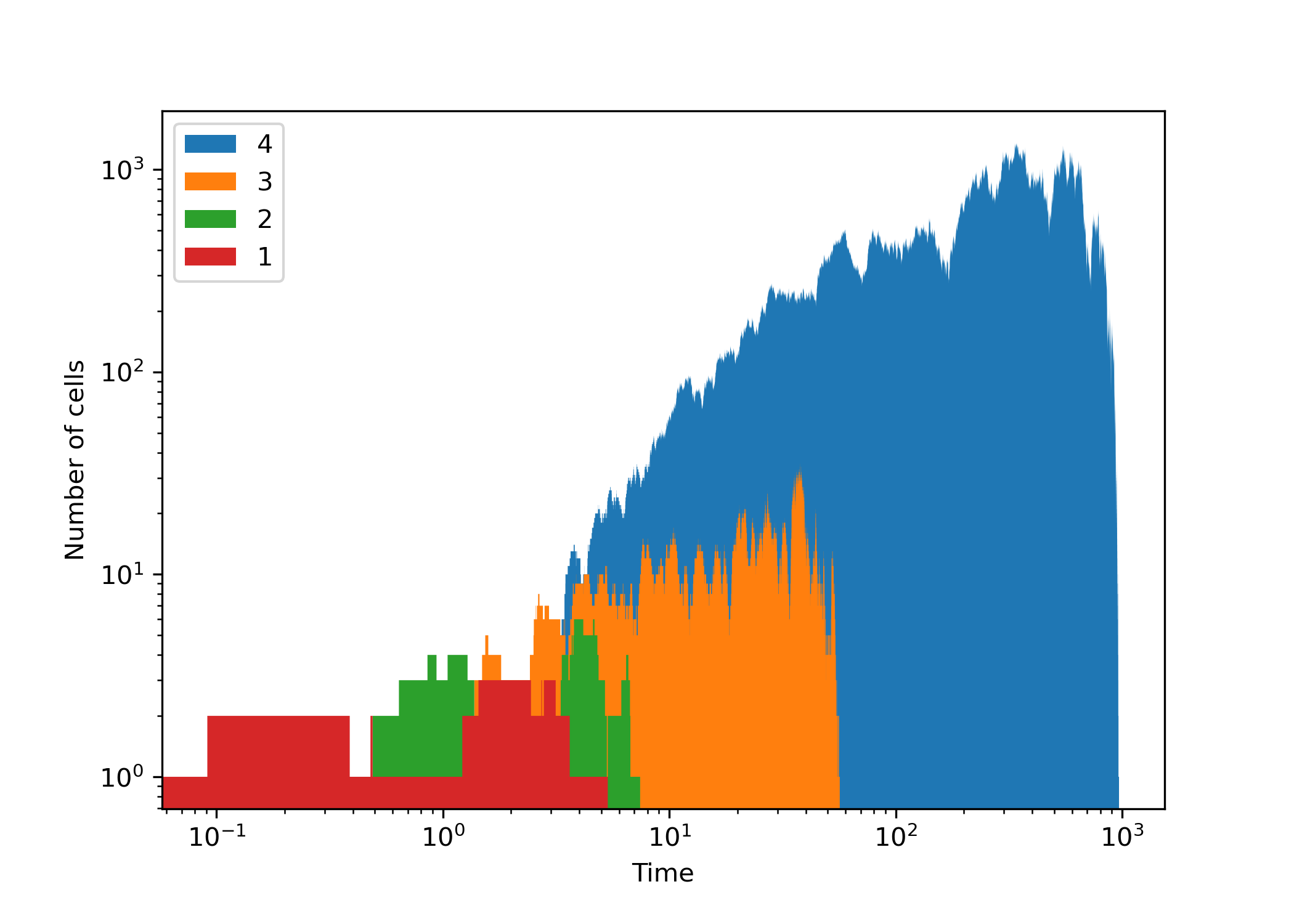
Figure 1. An example simulation run until extinction with n=4 types, where each colored area represents the number of cells of a type, with different types piled on top of each other. Hence the envelope is the total population size. A single initial type-1 cell resulted in a short-lived type-1 population which seeded a type-2 population before its extinction. Note how type-2 cells were initiated multiple times. One can observe the initial fast growth of the total population before extinction.

Since the behaviour of type $j$ cells doesn’t affect cell types up to $j-1$, the process is called decomposable. The asymptotic behavior of decomposable critical processes has been studied by many authors [30, 9, 23]. Foster and Ney [18] derived the asymptotic survival probability for discrete-time models. Similar results were obtained simultaneously by Ogura [25], also including continuous time processes. Later on, Foster and Ney [19] proposed limit theorems for the generating functions of population sizes, conditioned on the survival of the first type of cells, a condition less relevant when modeling error catastrophe.

Some time-independent properties of the $n$-type critical process of this paper have been explored in [5]. In that work, the process was interpreted as a model of an infection outbreak, and the outbreak size, that is, the total number of infected individuals of each type of disease ever produced was studied. In the present model the outbreak size corresponds to the total number of cells of each type ever produced, but counting a cell division as a production of just one new cell, as this refers to the infection of a new individual (and one also needs to account for the initial type-1 cell). It was possible to obtain the exact generating function for the type-$n$ outbreak size $N_{n}$. In particular, it was found that the mass function of the outbreak size for each type has power law tail, that is $P(N_{n}=a)\propto a^{-1-\chi_{n}/2}$ with $\chi_{n}=2^{1-n}$, implying infinite mean outbreak sizes. However, in order to study the evolution of cancer or bacteria populations, one is interested in the dynamics of the population in time, which is the focus of attention of this paper.

In this work, we derive large-time asymptotic solutions of multi-type critical birth-death processes exploiting the fact that, after an initial stage of exponential growth, the population is dominated by the last type. More precisely, we show that, for a large time, the system is non-empty with probability proportional to $(\text{time})^{-\chi_{n}}$, where $\chi_{n}=2^{1-n}$. The same exponents were derived by [18, 25] through a different approach. This allows us to find an appropriate scaling of the system, and derive the limiting distribution for the number of cells of a given type present at time $t$. We find asymptotic solutions for the distribution of cells of type $k=1,\dots,n$, as well as the total number distribution. Our methods extend the exact solution and limit results [4] for the two-type critical birth-death case, and complement the results of recent work on super-critical processes [24]. Remarkably, we find that the distributions for the number of cells of a given type and the total number distributions have algebraic and stationary tails, described by the same exponents $\chi_{n}$ as the survival probabilities. We derive further estimates of interest for studying cancer and bacteria growth, including the distributions of time of arrival and extinction of cells with an arbitrary number of mutations.

The next sections progressively build up to the main results of this work, which can be found in Section 5. We start by introducing the simplest critical processes in sections 2 and  3. We then present exact solutions to the two-type critical process in Section 4, and we finally derive asymptotic solutions to the $n$-type case in Section 5. In Appendix E we examine the more general processes including death and arbitrary birth and mutation rates, and we find that the behavior is essentially the same as in the simplest critical birth-death process. Therefore, in the bulk of the paper we limit ourselves to the simplest version. Some applications and interpretation of the results for studying error catastrophe in cancer and bacteria are considered in the discussion.

2. Single type

Let us recall the basic properties of a single type critical process [6]. We denote by $Z_{i}(t)$ the number of type-$i$ cells at time $t$. We start with a single type-1 cell and study $Z_{1}(t)$ via the generating function $\mathcal{Z}_{1,1}(x_{1},t)=\mathbb{E}(x_{1}^{Z_{1}(t)}|Z_{1}(0)=1)$, where the first index refers to the type of the initial cell and the second to the number of types considered. It can be obtained from the backward Kolmogorov equation $\partial_{t}\mathcal{Z}_{1,1}=(1-\mathcal{Z}_{1,1})^{2}$ with $\mathcal{Z}_{1,1}(x_{1},0)=x_{1}$, which leads to

(3) $$\mathcal{Z}_{1,1}(x_{1},t)=\frac{t(1-x_{1})+x_{1}}{t(1-x_{1})+1}.$$

By expanding this around $x_{1}=0$ we obtain the probability to have $a$ cells at time $t$, that is $P_{a}(t)=\mathbb{P}(Z_{1}(t)=a|Z_{1}(0)=1)$, which is

(4) $$P_{a}(t)=\frac{1}{(1+t)^{2}}\left(\frac{t}{1+t}\right)^{a-1}$$

for $a\geq 1$, and the survival probability

(5) $$S_{1,1}(t)=1-\mathcal{Z}_{1,1}(0,t)=1-P_{0}(t)=\frac{1}{1+t}.$$

Hence the number of cells conditioned on survival has a geometric distribution

$$Z_{1}(t)|\{Z_{1}(t)>0\}\sim\mathrm{Geo}\left(\frac{1}{1+t}\right).$$

Notice that the average number of cells remains constant,

$$\mathbb{E}Z_{1}(t)=\partial_{x_{1}}\mathcal{Z}_{1,1}(1,t)=\sum_{a\geq 1}aP_{a}(t)=1,$$

throughout the evolution. Although the probability of extinction for $t\to\infty$ is one, it takes a long time, since for $T=\inf\{t:Z_{1}(t)=0\}$,

$$\mathbb{E}T=\int_{0}^{\infty}\mathbb{P}(T>t)dt=\int_{0}^{\infty}S_{1,1}(t)dt=\infty.$$

It is well known [6] that conditioned on survival $Z_{1}(t)/t$ converges in distribution to an exponential random variable

(6) $$\frac{Z_{1}(t)}{t}|\{Z_{1}(t)>0\}\to Y_{1}\sim\mathrm{Expo}(1)$$

for $t\to\infty$. This is immediate from the properties of a geometric distribution when taking the limit $t,a\to\infty$ limit with $a/t=y$ constant

$$\mathbb{P}\left(\frac{Z_{1}(t)}{t}>y|Z_{1}(t)>0\right)=\left(\frac{t}{t+1}\right)^{ty}\to e^{-y}=\mathbb{P}(Y_{1}>y).$$

One can also derive this from the generating function. First note that $\mathbb{P}(Z_{1}(t)=a|Z_{1}(t)>0)=P_{a}(t)/S(t)$, hence the conditional generating function

(7) $$\mathbb{E}(x_{1}^{Z_{1}(t)}|Z_{1}(t)>0)=\sum_{a\geq 1}\frac{P_{a}(t)}{S(t)}x_{1}^{a}=\frac{\mathcal{Z}_{1,1}(x_{1},t)-P_{0}(t)}{1-P_{0}(t)}.$$

The large $a$ limit is related to $x_{1}\approx 1$ so, in order to get a non-trivial limit, we write $x_{1}=1-p/t$ with $p$ constant and notice that for $a,t\to\infty$, the right-hand side of (7) converges

$$\frac{\mathcal{Z}_{1,1}(1-p/t,t)-P_{0}(t)}{1-P_{0}(t)}=\frac{1-p/t}{1+p}\to\frac{1}{1+p}.$$

The convergence of (7) requres that $tP_{a}(t)/S(t)\sim t^{2}P_{a}(t)\to f_{Y_{1}}(y)$ in order to get

$$\sum_{a\geq 1}\frac{P_{a}(t)}{S(t)}x_{1}^{a}=\sum_{a\geq 1}t\frac{P_{a}(t)}{S(t)}\left(1-\frac{p}{t}\right)^{yt}\frac{1}{t}\to\int_{0}^{\infty}f_{Y_{1}}(y)e^{-py}dy=\mathbb{E}e^{pY_{1}}$$

to converge to the Riemann integral, which is the Laplace transform of the density $f_{Y}(y)$. The two limits are of course the same, hence

(8) $$\lim_{t\to\infty}\frac{\mathcal{Z}_{1,1}(1-p/t,t)-P_{0}(t)}{1-P_{0}(t)}=\mathbb{E}e^{pY_{1}}=\frac{1}{1+p}.$$

By inverting (8), the Laplace transform of the density $f_{Y_{1}}(y)$, we indeed obtain that $Y_{1}\sim\mathrm{Expo}(1)$.

3. Infinite types

An interesting special case is obtained when we consider infinitely many types ($n=\infty$) in the process described by scheme (1). If $n=\infty$, there is no extinction, but up to type $m$ the process is identical to the $m$-type model. What becomes simple though in the infinite type model is the total number of cells: if we disregard the types of cells then $Z(t)=\sum_{i\geq 1}Z_{i}(t)$ is a Yule process with rate one [6]. The generating function of a Yule process $\mathcal{Z}(x,t)=\mathbb{E}(x^{Z(t)}|Z(0)=1)$ can be obtained from the backward Kolmogorov equation $\partial_{t}\mathcal{Z}=\mathcal{Z}(\mathcal{Z}-1)$ with $\mathcal{Z}(x,0)=x$, which leads to

$$\mathcal{Z}(x,t)=\frac{x}{x+(1-x)e^{t}}.$$

By expanding this around $x=0$, we obtain the mass function of the total number of cells in the infinite type process with a single initial type-1 cell

$$\Pi_{s}(t)=\mathbb{P}(Z(t)=s|Z_{i}(t)=\delta_{i1})=e^{-t}\big{(}1-e^{-t}\big{)}^{s-1}.$$

The mean number of cells grows exponentially as $\mathbb{E}Z(t)=\partial_{x}\mathcal{Z}(1,t)=e^{t}$. For finite multi-type critical branching processes, $\Pi_{s}(t)$ is not known in general. This is addressed in the next sections.

4. Two types

Consider now the simplest two-type critical branching process, represented by

(9) $$\begin{split}\lx@xy@svg{\hbox{\raise 0.0pt\hbox{\kern 21.88889pt\hbox{\ignorespaces\ignorespaces\ignorespaces\hbox{\vtop{\kern 0.0pt\offinterlineskip\halign{\entry@#!@&&\entry@@#!@\cr&&\\&&\crcr}}}\ignorespaces{\hbox{\kern-21.88889pt\raise 0.0pt\hbox{\hbox{\kern 0.0pt\raise 0.0pt\hbox{\hbox{\kern 3.0pt\raise 0.0pt\hbox{$\textstyle{(1)+(1)}$}}}}}}}{\hbox{\kern 45.88889pt\raise 0.0pt\hbox{\hbox{\kern 0.0pt\raise 0.0pt\hbox{\hbox{\kern 3.0pt\raise 0.0pt\hbox{$\textstyle{(2)+(2)}$}}}}}}}{\hbox{\kern 116.16666pt\raise 0.0pt\hbox{\hbox{\kern 0.0pt\raise 0.0pt\hbox{\hbox{\kern 3.0pt\raise 0.0pt\hbox{$\textstyle{}$}}}}}}}{\hbox{\kern-9.3889pt\raise-40.0pt\hbox{\hbox{\kern 0.0pt\raise 0.0pt\hbox{\hbox{\kern 3.0pt\raise 0.0pt\hbox{$\textstyle{(1)\ignorespaces\ignorespaces\ignorespaces\ignorespaces\ignorespaces\ignorespaces\ignorespaces\ignorespaces}$}}}}}}}\ignorespaces\ignorespaces\ignorespaces\ignorespaces{}{\hbox{\lx@xy@droprule}}\ignorespaces{\hbox{\kern 0.0pt\raise-5.5pt\hbox{\hbox{\kern 0.0pt\raise 0.0pt\hbox{\lx@xy@tip{1}\lx@xy@tip{-1}}}}}}{\hbox{\lx@xy@droprule}}{\hbox{\lx@xy@droprule}}\ignorespaces\ignorespaces\ignorespaces\ignorespaces{}{\hbox{\lx@xy@droprule}}\ignorespaces{\hbox{\kern 58.38887pt\raise-40.0pt\hbox{\hbox{\kern 0.0pt\raise 0.0pt\hbox{\lx@xy@tip{1}\lx@xy@tip{-1}}}}}}{\hbox{\lx@xy@droprule}}{\hbox{\lx@xy@droprule}}{\hbox{\kern 58.38887pt\raise-40.0pt\hbox{\hbox{\kern 0.0pt\raise 0.0pt\hbox{\hbox{\kern 3.0pt\raise 0.0pt\hbox{$\textstyle{(2)\ignorespaces\ignorespaces\ignorespaces\ignorespaces\ignorespaces\ignorespaces\ignorespaces\ignorespaces}$}}}}}}}\ignorespaces\ignorespaces\ignorespaces\ignorespaces{}{\hbox{\lx@xy@droprule}}\ignorespaces{\hbox{\kern 67.77777pt\raise-5.5pt\hbox{\hbox{\kern 0.0pt\raise 0.0pt\hbox{\lx@xy@tip{1}\lx@xy@tip{-1}}}}}}{\hbox{\lx@xy@droprule}}{\hbox{\lx@xy@droprule}}\ignorespaces\ignorespaces\ignorespaces\ignorespaces{}{\hbox{\lx@xy@droprule}}\ignorespaces{\hbox{\kern 113.66666pt\raise-40.0pt\hbox{\hbox{\kern 0.0pt\raise 0.0pt\hbox{\lx@xy@tip{1}\lx@xy@tip{-1}}}}}}{\hbox{\lx@xy@droprule}}{\hbox{\lx@xy@droprule}}{\hbox{\kern 113.66666pt\raise-40.0pt\hbox{\hbox{\kern 0.0pt\raise 0.0pt\hbox{\hbox{\kern 3.0pt\raise 0.0pt\hbox{$\textstyle{\emptyset}$}}}}}}}\ignorespaces}}}}\ignorespaces\end{split} \textstyle{(1)+(1)} \textstyle{(2)+(2)} \textstyle{(1)\ignorespaces\ignorespaces\ignorespaces\ignorespaces\ignorespaces\ignorespaces\ignorespaces\ignorespaces} \textstyle{(2)\ignorespaces\ignorespaces\ignorespaces\ignorespaces\ignorespaces\ignorespaces\ignorespaces\ignorespaces} \textstyle{\emptyset} \textstyle{(1)+(1)} \textstyle{(2)+(2)} \textstyle{(1)\ignorespaces\ignorespaces\ignorespaces\ignorespaces\ignorespaces\ignorespaces\ignorespaces\ignorespaces} \textstyle{(2)\ignorespaces\ignorespaces\ignorespaces\ignorespaces\ignorespaces\ignorespaces\ignorespaces\ignorespaces} \textstyle{\emptyset}$$

where all steps occur at equal rates; we set these rates to unity for simplicity. The general case is considered in Appendix A. While the single type birth-death process is easily soluble, the two-type birth-death process reduces to generally unsolvable Riccati equations, which were recently shown to be solvable for certain birth-death models with general rates [3, 4]. For the critical case, the situation slightly simplifies and the results are more explicit. Although the analytic solution for the two-type critical case was published in [4], here we re-derive the solution in more detail. These exact results will be useful for checking the validity of the asymptotic results we derive in Section 5 for general $n$, which is the only available approach for $n\geq 3$.

Since the process is decomposable, the generating function for type-$1$ cells is the same as in the single type process given in (3). The generating function for both cell types, starting with a single initial type-i cell is

(10) $$\mathcal{Z}_{i,2}(x_{1},x_{2},t)=\mathbb{E}(x_{1}^{Z_{1}(t)}x_{2}^{Z_{2}(t)}|Z_{j}(t)=\delta_{ij})$$

for $i=1,2$, and hence the initial conditions are

(11a) $$\mathcal{Z}_{1,2}(x_{1},x_{2},0) =x_{1}$$

(11b) $$\mathcal{Z}_{2,2}(x_{1},x_{2},0) =x_{2}.$$

A convenient setting for studying the two-type branching process is provided by the backward Kolmogorov equations

(12a) $$\partial_{t}\mathcal{Z}_{1,2} =\mathcal{Z}_{1,2}^{2}+\mathcal{Z}_{2,2}-2\mathcal{Z}_{1,2}$$

(12b) $$\partial_{t}\mathcal{Z}_{2,2} =\mathcal{Z}_{2,2}^{2}+1-2\mathcal{Z}_{2,2}.$$

Let $\sigma$ be an operator that increases the indices of a function by one,

(13) $$\sigma(\mathcal{F}_{i,j}(x_{i},x_{j}))=\mathcal{F}_{i+1,j+1}(x_{i+1},x_{j+1}).$$

Note that in the general case (see Appendix E) $\sigma$ increases the indices of the rates $\alpha_{i},\chi_{i},\nu_{i}$ too. Since we are considering decomposable processes, one can easily see that $\mathcal{Z}_{i+1,j+1}=\sigma(\mathcal{Z}_{i,j})$, namely the $j$-type process starting with a single $i$ cell is the same as the $j+1$ process starting with a single $i+1$ cell, up to a change in indices. In particular, $\mathcal{Z}_{2,2}=\sigma(\mathcal{Z}_{1,1})$, where $\mathcal{Z}_{1,1}$ is the generating function of the single type process, given in (3).

4.1. Survival probabilities

Before solving Eqs. (12a)–(12b), we consider the simpler task of finding the survival probability of the system, where ‘survival’ refers to the situation when there are alive cells of any type at time $t$,

$$S_{i,2}(t)=\mathbb{P}(Z_{1}(t)+Z_{2}(t)>0|Z_{k}(0)=\delta_{i,k}).$$

The survival probabilities are related to the corresponding generating functions for type-two cells, $S_{1,2}(t)=1-\mathcal{Z}_{1,2}(0,0,t)$ and $S_{2,2}(t)=1-\mathcal{Z}_{2,2}(0,0,t)$. Hence from Eqs. (12a)–(12b) we deduce that the survival probabilities $S_{1,2}(t)$ and $S_{2,2}(t)$ evolve according to rate equations

(14a) $$\frac{dS_{1,2}}{dt} =S_{2,2}-S_{1,2}^{2}$$

(14b) $$\frac{dS_{2,2}}{dt} =-S_{2,2}^{2},$$

with initial conditions $S_{1,2}(0)=S_{2,2}(0)=1$. Note that

(15) $$S_{2,2}=\sigma(S_{1,1})=S_{1,1}=\frac{1}{1+t}$$

is the survival of the single type process, given by (5). The governing equation (14a) therefore becomes a initial value problem

(16) $$\frac{dS_{1,2}}{dt}=\frac{1}{1+t}-S_{1,2}^{2},\quad S_{1,2}(0)=1.$$

This is a soluble Riccati equation. We first simplify the non-homogeneous term by using the new time variable $\tau=\sqrt{1+t}$, which leads to

$$\frac{dS_{1,2}}{d\tau}=\frac{2}{\tau}-2\tau S_{1,2}^{2}.$$

We transform this into a second-order linear differential equation by setting $S_{1,2}(\tau)=\frac{1}{2\tau}\frac{B^{\prime}(\tau)}{B(\tau)}$ to get

$$B^{\prime\prime}(\tau)-\frac{B^{\prime}(\tau)}{\tau}-4B(\tau)=0.$$

Finally, we let $s=2\tau$ and write $B(\tau)=\frac{s}{2}A(s)$ to obtain the standard differential equation for modified Bessel functions [10]

$$s^{2}A^{\prime\prime}(s)+sA^{\prime}(s)-(1+s^{2})A(s)=0.$$

Hence the solution is a linear combination of these functions

$$A(t)=c_{1}I_{0}(t)+c_{2}K_{0}(t),$$

where $I_{p}$ and $K_{p}$ are the modified Bessel functions of order $p$ of the first and second kind, respectively. Making the previous substitutions backward, we arrive at the solution of (16)

(17) $$S_{1,2}=\frac{1}{\tau}\,\frac{I_{0}(2\tau)-cK_{0}(2\tau)}{I_{1}(2\tau)+cK_{1}(2\tau)}\,,\quad\tau=\sqrt{1+t}.$$

The initial condition $S_{1,2}(t=0)=1$ fixes the amplitude

(18) $$c=\frac{I_{0}(2)-I_{1}(2)}{K_{0}(2)+K_{1}(2)}.$$

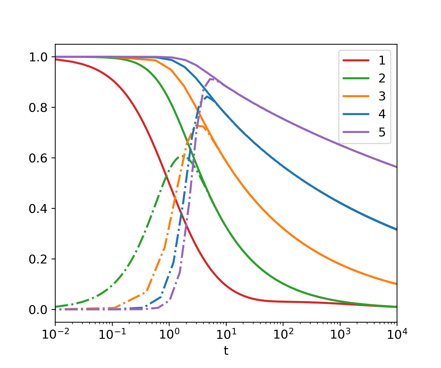
Figure 2. Survival probabilities of the n-type critical process with initial condition $Z_{1}(0)=1$. We plot the survival probability of the entire system, $S_{1,n}(t)$ (lines) and that of just type-$n$ cells, $Q_{1,n}(t)$ (dashed-dots lines). Curves are for different types $n=1,\dots,5$. For 1 and 2-type cells, the solutions are exact from (3) and (22), respectively. For other $n>2$, solutions are obtained numerically from (31) with different initial conditions.

4.2. Generating functions

We now return to the generating functions $\mathcal{Z}_{1,2}$ and $\mathcal{Z}_{2,2}$. A full solution of Eqs. (12a)–(12b) subject to the initial conditions (11a)–(11b) is obtained in similar way as the above solution of Eqs. (12a)–(12b). First, notice that the solution of (12b) is just the generating function (3) of a single type but with the indexes increased by one

(19) $$\mathcal{Z}_{2,2}=\sigma(\mathcal{Z}_{1,1})=\frac{t(1-x_{2})+x_{2}}{t(1-x_{2})+1}.$$

Plugging this into (12a) we recast it into a Riccati equation

(20) $$\frac{d(1-\mathcal{Z}_{1,2})}{dt}=\frac{1}{(1-x_{2})^{-1}+t}-(1-\mathcal{Z}_{1,2})^{2}.$$

Comparing (20) and (16) we see that $1-\mathcal{Z}_{1,2}$ satisfies the same equation as $S_{1,2}$, the only distinction is in the shift of the time variable in the first term on the right-hand sides. Thus we use the variable

(21) $$\tau=\sqrt{t+(1-x_{2})^{-1}}.$$

and then the solution becomes

(22) $$\mathcal{Z}_{1,2}=1-\frac{1}{\tau}\,\frac{I_{0}(2\tau)-cK_{0}(2\tau)}{I_{1}(2\tau)+cK_{1}(2\tau)},$$

where the initial condition $\mathcal{Z}_{1,2}(x_{1},x_{2},0)=x_{1}$ gives the amplitude

(23) $$c=\frac{I_{0}(2\tau_{0})-(1-x_{1})\tau_{0}I_{1}(2\tau_{0})}{K_{0}(2\tau_{0})+(1-x_{1})\tau_{0}K_{1}(2\tau_{0})}.$$

where

(24) $$\tau_{0}=\frac{1}{\sqrt{1-x_{2}}}.$$

For $x_{1}=x_{2}=0$ we recover the survival probabilities (17).

Having a full solution (22)–(24) for the generating function, we can extract the probability of finding $a$ type-1 cells and $b$ type-2 cells, $P_{a,b}(t)$, by using Cauchy’s integral formula:

(25) $$P_{a,b}(t)=\frac{1}{(2\pi i)^{2}}\oint\frac{dx_{1}}{x_{1}^{a+1}}\oint\frac{dx_{2}}{x_{2}^{b+1}}\,\mathcal{Z}_{1,2}(x_{1},x_{2},t).$$

Unfortunately, explicit solutions for $P_{a,b}(t)$ are not available for arbitrary $a$ and $b$, although one can reduce the number of integrations in Eq. (25) to one, and use numerical methods to obtain values for arbitrary $a$ and $b$, see Appendix B and C. Fortunately, in many applications, a less detailed description suffices. For instance, one may be interested in the marginal distribution of type-2 cells,

$$P^{(2)}_{s}(t)=\mathbb{P}(Z_{2}(t)=s)$$

or the total population size of the two-type process

$$\Pi^{(2)}_{s}(t)=\mathbb{P}(Z_{1}(t)+Z_{2}(t)=s).$$

These are encoded in the generating functions

(26) $$\mathcal{Z}_{1,2}(1,x,t) =\mathbb{E}(x^{Z_{2}(t)}|Z_{j}(0)=\delta_{1j})=\sum_{s\geq 0}P^{(2)}_{s}(t)x^{s}$$

(27) $$\mathcal{Z}_{1,2}(x,x,t) =\mathbb{E}(x^{Z_{1}(t)+Z_{2}(t)}|Z_{j}(0)=\delta_{1j})=\sum_{s\geq 0}\Pi^{(2)}_{s}(t)x^{s}.$$

In the next section, we derive the asymptotic behaviour of both distributions.

5. $n$ types

In this section, we study the $n-$type critical birth-death process, represented by the scheme

$$\begin{split}\lx@xy@svg{\hbox{\raise 0.0pt\hbox{\kern 21.88889pt\hbox{\ignorespaces\ignorespaces\ignorespaces\hbox{\vtop{\kern 0.0pt\offinterlineskip\halign{\entry@#!@&&\entry@@#!@\cr&&&&\\&&&&\crcr}}}\ignorespaces{\hbox{\kern-21.88889pt\raise 0.0pt\hbox{\hbox{\kern 0.0pt\raise 0.0pt\hbox{\hbox{\kern 3.0pt\raise 0.0pt\hbox{$\textstyle{(1)+(1)}$}}}}}}}{\hbox{\kern 45.88889pt\raise 0.0pt\hbox{\hbox{\kern 0.0pt\raise 0.0pt\hbox{\hbox{\kern 3.0pt\raise 0.0pt\hbox{$\textstyle{(2)+(2)}$}}}}}}}{\hbox{\kern 117.41666pt\raise 0.0pt\hbox{\hbox{\kern 0.0pt\raise 0.0pt\hbox{\hbox{\kern 3.0pt\raise 0.0pt\hbox{$\textstyle{}$}}}}}}}{\hbox{\kern 151.16666pt\raise 0.0pt\hbox{\hbox{\kern 0.0pt\raise 0.0pt\hbox{\hbox{\kern 3.0pt\raise 0.0pt\hbox{$\textstyle{(n)+(n)}$}}}}}}}{\hbox{\kern 223.4491pt\raise 0.0pt\hbox{\hbox{\kern 0.0pt\raise 0.0pt\hbox{\hbox{\kern 3.0pt\raise 0.0pt\hbox{$\textstyle{}$}}}}}}}{\hbox{\kern-9.3889pt\raise-40.0pt\hbox{\hbox{\kern 0.0pt\raise 0.0pt\hbox{\hbox{\kern 3.0pt\raise 0.0pt\hbox{$\textstyle{(1)\ignorespaces\ignorespaces\ignorespaces\ignorespaces\ignorespaces\ignorespaces\ignorespaces\ignorespaces}$}}}}}}}\ignorespaces\ignorespaces\ignorespaces\ignorespaces{}{\hbox{\lx@xy@droprule}}\ignorespaces{\hbox{\kern 0.0pt\raise-5.5pt\hbox{\hbox{\kern 0.0pt\raise 0.0pt\hbox{\lx@xy@tip{1}\lx@xy@tip{-1}}}}}}{\hbox{\lx@xy@droprule}}{\hbox{\lx@xy@droprule}}\ignorespaces\ignorespaces\ignorespaces\ignorespaces{}{\hbox{\lx@xy@droprule}}\ignorespaces{\hbox{\kern 58.38887pt\raise-40.0pt\hbox{\hbox{\kern 0.0pt\raise 0.0pt\hbox{\lx@xy@tip{1}\lx@xy@tip{-1}}}}}}{\hbox{\lx@xy@droprule}}{\hbox{\lx@xy@droprule}}{\hbox{\kern 58.38887pt\raise-40.0pt\hbox{\hbox{\kern 0.0pt\raise 0.0pt\hbox{\hbox{\kern 3.0pt\raise 0.0pt\hbox{$\textstyle{(2)\ignorespaces\ignorespaces\ignorespaces\ignorespaces\ignorespaces\ignorespaces\ignorespaces\ignorespaces}$}}}}}}}\ignorespaces\ignorespaces\ignorespaces\ignorespaces{}{\hbox{\lx@xy@droprule}}\ignorespaces{\hbox{\kern 67.77777pt\raise-5.5pt\hbox{\hbox{\kern 0.0pt\raise 0.0pt\hbox{\lx@xy@tip{1}\lx@xy@tip{-1}}}}}}{\hbox{\lx@xy@droprule}}{\hbox{\lx@xy@droprule}}\ignorespaces\ignorespaces\ignorespaces\ignorespaces{}{\hbox{\lx@xy@droprule}}\ignorespaces{\hbox{\kern 113.66666pt\raise-40.0pt\hbox{\hbox{\kern 0.0pt\raise 0.0pt\hbox{\lx@xy@tip{1}\lx@xy@tip{-1}}}}}}{\hbox{\lx@xy@droprule}}{\hbox{\lx@xy@droprule}}{\hbox{\kern 113.66666pt\raise-40.0pt\hbox{\hbox{\kern 0.0pt\raise 0.0pt\hbox{\hbox{\kern 3.0pt\raise 0.0pt\hbox{$\textstyle{\cdots\ignorespaces\ignorespaces\ignorespaces\ignorespaces}$}}}}}}}\ignorespaces\ignorespaces\ignorespaces\ignorespaces{}{\hbox{\lx@xy@droprule}}\ignorespaces{\hbox{\kern 164.1678pt\raise-40.0pt\hbox{\hbox{\kern 0.0pt\raise 0.0pt\hbox{\lx@xy@tip{1}\lx@xy@tip{-1}}}}}}{\hbox{\lx@xy@droprule}}{\hbox{\lx@xy@droprule}}{\hbox{\kern 164.1678pt\raise-40.0pt\hbox{\hbox{\kern 0.0pt\raise 0.0pt\hbox{\hbox{\kern 3.0pt\raise 0.0pt\hbox{$\textstyle{(n)\ignorespaces\ignorespaces\ignorespaces\ignorespaces\ignorespaces\ignorespaces\ignorespaces\ignorespaces}$}}}}}}}\ignorespaces\ignorespaces\ignorespaces\ignorespaces{}{\hbox{\lx@xy@droprule}}\ignorespaces{\hbox{\kern 174.05788pt\raise-5.5pt\hbox{\hbox{\kern 0.0pt\raise 0.0pt\hbox{\lx@xy@tip{1}\lx@xy@tip{-1}}}}}}{\hbox{\lx@xy@droprule}}{\hbox{\lx@xy@droprule}}\ignorespaces\ignorespaces\ignorespaces\ignorespaces{}{\hbox{\lx@xy@droprule}}\ignorespaces{\hbox{\kern 220.9491pt\raise-40.0pt\hbox{\hbox{\kern 0.0pt\raise 0.0pt\hbox{\lx@xy@tip{1}\lx@xy@tip{-1}}}}}}{\hbox{\lx@xy@droprule}}{\hbox{\lx@xy@droprule}}{\hbox{\kern 220.9491pt\raise-40.0pt\hbox{\hbox{\kern 0.0pt\raise 0.0pt\hbox{\hbox{\kern 3.0pt\raise 0.0pt\hbox{$\textstyle{\emptyset}$}}}}}}}\ignorespaces}}}}\ignorespaces\end{split} \textstyle{(1)+(1)} \textstyle{(2)+(2)} \textstyle{(n)+(n)} \textstyle{(1)\ignorespaces\ignorespaces\ignorespaces\ignorespaces\ignorespaces\ignorespaces\ignorespaces\ignorespaces} \textstyle{(2)\ignorespaces\ignorespaces\ignorespaces\ignorespaces\ignorespaces\ignorespaces\ignorespaces\ignorespaces} \textstyle{\cdots\ignorespaces\ignorespaces\ignorespaces\ignorespaces} \textstyle{(n)\ignorespaces\ignorespaces\ignorespaces\ignorespaces\ignorespaces\ignorespaces\ignorespaces\ignorespaces} \textstyle{\emptyset} \textstyle{(1)+(1)} \textstyle{(2)+(2)} \textstyle{(n)+(n)} \textstyle{(1)\ignorespaces\ignorespaces\ignorespaces\ignorespaces\ignorespaces\ignorespaces\ignorespaces\ignorespaces} \textstyle{(2)\ignorespaces\ignorespaces\ignorespaces\ignorespaces\ignorespaces\ignorespaces\ignorespaces\ignorespaces} \textstyle{\cdots\ignorespaces\ignorespaces\ignorespaces\ignorespaces} \textstyle{(n)\ignorespaces\ignorespaces\ignorespaces\ignorespaces\ignorespaces\ignorespaces\ignorespaces\ignorespaces} \textstyle{\emptyset}$$

This considers a decomposable critical process in which each type can only be produced by the preceding type, and all types divide or mutate at rate one, except the maximal type $n$ cells, which cannot mutate but die at rate one. The results can easily be generalized to consider more general cases including death and multiple mutation rates- the derivations can be found in the Appendix E.

The naïve approach to the problem is to study $\mathbb{E}Z_{i}(t)$. The forward equations are $\frac{d}{dt}\mathbb{E}Z_{1}(t)=0$ and

$$\frac{d}{dt}\mathbb{E}Z_{i}(t)=\mathbb{E}Z_{i-1}(t)$$

for $i=2,\dots n$, with initial condition $\mathbb{E}Z_{i}(0)=\delta_{i1}$. The solution is

(28) $$\mathbb{E}Z_{i}(t)=\frac{t^{i-1}}{(i-1)!}.$$

For the infinite type case ($n\to\infty$) we recover the Yule process of Section 3 for the total number of cells $\mathbb{E}Z(t)=\sum_{i\geq 1}\mathbb{E}Z_{i}(t)=e^{t}$. For a finite number of types, the mean total number of cells is $\mathbb{E}Z(t)\approx e^{t}$ for small $t$ but grow algebraically as $t^{n-1}$ when $t\to\infty$. Thus, even though the process is critical and dies out at a finite time with probability one, $\mathbb{E}Z(t)$ keeps growing forever, and therefore the naïve approach fails to capture one important aspect of the system. Hence instead of working with the mean number of cells, we derive asymptotic solutions for large time limits following a similar strategy introduced for the single type process.

The generating function for the $n$-type cell process starting with a single initial type-$i$ cell is

(29) $$\mathcal{Z}_{i,n}(x_{1},x_{2},\dots x_{n},t)=\mathbb{E}\left(\prod_{j=1}^{n}x_{j}^{Z_{j}(t)}|Z_{k}(t)=\delta_{ik}\right)$$

which can be obtained by solving the backward Kolmogorov equations

(30) $$\partial_{t}\mathcal{Z}_{i,n}=\begin{cases}\mathcal{Z}_{i,n}^{2}+\mathcal{Z}_{i+1,n}-2\mathcal{Z}_{i,n}&\text{for}\quad{i=1,\dots,n-1}\\ \mathcal{Z}_{i,n}^{2}+1-2\mathcal{Z}_{i,n}&\text{for}\quad{i=n}.\end{cases}$$

Thus, in order to obtain the interesting generating function $\mathcal{Z}_{1,n}$ for the $n$-type process starting from a single type-$1$ cell, we need to first solve the $n-1$ equations for $\mathcal{Z}_{n,n},\mathcal{Z}_{n-1,n},\dots,\mathcal{Z}_{2,n}$. However, since the system is decomposable, we have that $\mathcal{Z}_{i+1,j+1}=\sigma(\mathcal{Z}_{i,j})$, where $\sigma()$ is the index increase operator (13). Thus, if we know the generating function for type-$k$ cells, solving the system for $k+1$ involves solving a single additional equation. For example, for the 3-type process, $\mathcal{Z}_{3,3}=\sigma(\mathcal{Z}_{2,2})$ and $\mathcal{Z}_{2,3}=\sigma(\mathcal{Z}_{1,2})$, which we solved in the $2$-type process, and thus we only need to solve one more equation in order to obtain $\mathcal{Z}_{1,3}$. The same applies to the survival probabilities, which we consider in the following section.

5.1. Survival probabilities

As seen in Section 4, it is simpler to solve the system for the survival probabilities

$$S_{i,n}(t)=\mathbb{P}(Z_{1}(t)+\dots+Z_{n}(t)>0|Z_{k}(0)=\delta_{i,k})=1-\mathcal{Z}_{i,n}(0,0,\dots,0,t).$$

Substituting into (30), we deduce that

(31) $$\frac{dS_{i,n}}{dt}=\begin{cases}S_{i+1,n}-{S_{i,n}}^{2}\quad&\text{for}\quad{i=1,\dots,n-1},\\ -S_{n,n}^{2}\quad&\text{for}\quad{i=n},\end{cases}$$

with initial conditions $S_{i,n}(0)=1$ for all $i=1,\dots,n$. For any $n$, the solutions starting with a single $n$-type cell are given by the solutions of the single-type system up to shift in indices,

$$S_{n,n}=\sigma(S_{n-1,n-1})=\dots=\sigma(S_{2,2})=\sigma(S_{1,1})=1/(1+t).$$

To get $S_{n-1,n}$, we need to solve

(32) $$\frac{dS_{n-1,n}}{dt}=\frac{1}{1+t}-{S^{2}_{n-1,n}}.$$

We have solved this case in Section 4.1 exactly, where we specified $n=2$, but the solution’s form is the same for all $n$. Even though analytic solutions are invaluable, the most interesting long-time asymptotic behavior can be extracted directly from the above equation, circumventing the exact solutions. Assume that asymptotically $S_{n-1,n}\sim(1+t)^{-\alpha}$, with $\alpha>0$. Substituting into (32) we get

$$-\alpha(1+t)^{-\alpha-1}\sim(1+t)^{-1}-(1+t)^{-2\alpha}$$

which leads to a contradiction for both $2\alpha>1$ and $2\alpha<1$. This shows that $2\alpha=1$, that is in the leading order the right-hand side of (32) should vanish faster than $1/(1+t)$. This gives

(33) $$S_{n-1,n}\sim(1+t)^{-1/2}.$$

To get higher-order terms we just add new terms one by one and match coefficients to get

(34) $$S_{n-1,n}\sim(1+t)^{-1/2}+\tfrac{1}{4}(1+t)^{-1}+\tfrac{3}{32}(1+t)^{-3/2}.$$

Note that we performed the expansion in powers of $1+t$ for convenience, but one could simply expand the result in powers of $t$ instead. This expansion can be also derived from the exact formula (17) using large argument asymptotic expansion of the Bessel functions (Appendix D).

Continuing to the next type, we have the differential equation for $S_{n-2,n}$ in (31) where $S_{n-1,n}$ is replaced by its above expansion. This procedure gives the leading order for all types by setting the time derivative to zero. In the leading order, we get that $S_{n-j,n}\sim(1+t)^{-\chi_{j+1}}$ with $\chi_{j}=2^{1-j}$. With a little more work one obtains the next correction

$$S_{n-j,n}\sim{(1+t)}^{-\chi_{j+1}}+2^{-j-1}{(1+t)}^{-\tfrac{1}{2}-\chi_{j+1}}$$

for $j=1,\dots,n-1$. The most interesting survival probability is $S_{1,n}$, which gives the probability that the $n$-type system starting with a single type-1 cell is not empty at time $t$. Asymptotically, this is given by

(35) $$S_{1,n}\sim(1+t)^{-\chi_{n}}+\frac{\chi_{n}}{2}{(1+t)}^{-\tfrac{1}{2}-\chi_{n}}$$

for $n\geq 2$, and for $n=1$ the first term is exact. One can consider higher-order terms by successively adding terms and matching coefficients. Figure 3 shows that the second-order asymptotic accurately describes the behaviour.

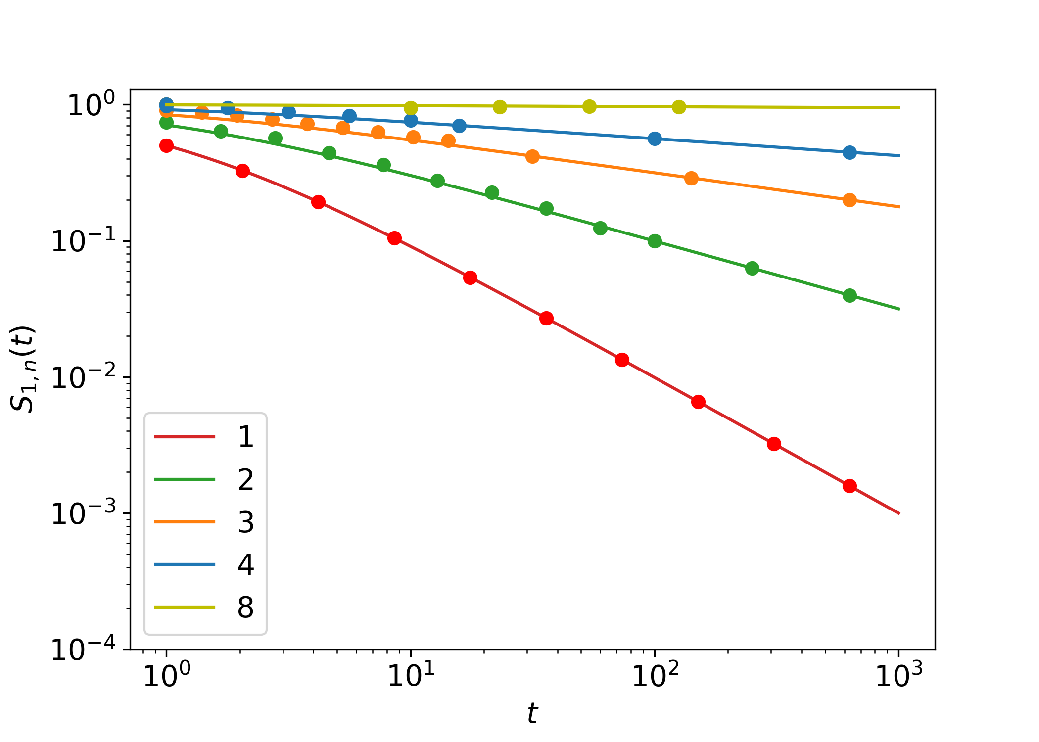
Figure 3. Survival probability of the n-type process, for $n=1,2,3,4,8$. Second-order asymptotic solutions obtained from (35) (lines) are plotted together with results from simulations (dots).

5.2. Generating functions

We now attempt to find solutions for the generating functions for the number of cells. We rewrite the Kolmogorov equations (29) into

(36) $$\frac{d(1-\mathcal{Z}_{i,n})}{dt}=\begin{cases}(1-\mathcal{Z}_{i+1,n})-(1-\mathcal{Z}_{i,n})^{2}\quad&\text{for}\quad{i=1,\dots,n-1},\\ -(1-\mathcal{Z}_{i,n})^{2}\quad&\text{for}\quad{i=n},\end{cases}$$

which for $1-\mathcal{Z}_{{j,n}}$ are identical to equations for the survival probability (31), but with initial conditions $1-\mathcal{Z}_{j,n}(x_{1},\dots,x_{n},0)=1-x_{j}$. This is not surprising since the survival probability is $S_{i,n}(t)=1-\mathcal{Z}_{i,n}(0,\dots 0,t)$.

We start solving this system again by considering the generating function for the system starting with a single type-$n$ cell, which corresponds to the single type case of, hence

$$1-\mathcal{Z}_{n,n}=\frac{1}{t+(1-x_{n})^{-1}},$$

which is the same as if we replace $1+t$ in $S_{n,n}$ by $t+(1-x_{n})^{-1}$. Starting with a single $(n-1)$ type cell we have

(37) $$\frac{d(1-\mathcal{Z}_{n-1,n})}{dt}=\frac{1}{t+(1-x_{n})^{-1}}-(1-\mathcal{Z}_{n-1,n})^{2}.$$

To get a nontrivial large-time behaviour we need $(1-x_{n})^{-1}\propto t$. Noting the similarity between (37) and (32), we assume a power behavior for $1-\mathcal{Z}_{n-1,n}$ which fixes the exponent and leads to

$$1-\mathcal{Z}_{n-1,n}\sim{\left({t+(1-x_{n})^{-1}}\right)}^{-1/2}.$$

Note that the same result can be also obtained directly from the explicit solution (22) for the generating function of type-2 cells $\mathcal{Z}_{1,2}(1,x_{2},t)$ by taking the large argument asymptotic of the modified Bessel functions [4].

Continuing this procedure we get that, to the leading order,

$$1-\mathcal{Z}_{n-2,n}\sim{\left({t+(1-x_{n})^{-1}}\right)}^{-1/4},$$

and so on. In particular, the generating function starting with a single type-1 cell is given by

(38) $$\mathcal{Z}_{1,n}\sim{\left({t+(1-x_{n})^{-1}}\right)}^{-\chi_{n}}.$$

Thus we see that the same exponents, $\chi_{n}=2^{1-n}$, that describe the survival probabilities give the asymptotic behaviour of the generating functions. Note that in the leading order, the generating functions only depend on the last type of cells $x_{n}$. This is not surprising if we note that the survival probability of type $k$ is the square root of the survival probability of type $k-1$, thus the system becomes dominated by the last type. A consequence of this is that

(39) $$\mathcal{Z}_{1,n}(1,\dots,1,x_{n},t)\sim\mathcal{Z}_{1,n}(x_{n},\dots,x_{n},t)$$

that is, the generating function for the last type is asymptotically the same as the generating function for the total number of cells.

If we take (39) at $x_{n}=0$ we see that the survival probability of just the type $n$ cells

$$Q_{i,n}(t)=\mathbb{P}(Z_{n}(t)>0|Z_{k}(0)=\delta_{i,k})=1-\mathcal{Z}_{i,n}(1,\dots,1,0,t)$$

is asymptotically the same as the survival probability of $S_{1,n}(t)$ of the whole system, that is

$$Q_{1,n}(t)\sim S_{1,n}(t).$$

This can be seen in Figure 2, where we plotted exact ($n=1,2$) and numerical ($n>2$) solutions for $S_{1,n}(t)$ and $Q_{1,n}(t)$. It is clear from (30) that $Q_{i,n}(t)$ is governed by the same equations as the survival probability $S_{i,n}(t)$ of the entire system (31) but with initial conditions $Q_{i,n}(0)=0$ for $i=2,\dots,n-1$ and $Q_{n,n}(0)=1$. In Figure 2 we see that subsequent types arise fast but disappear slowly, as the system gets dominated by the last type.

5.3. Cell number distributions

We now derive the asymptotic distribution of the $n$-type cells

$$P^{(n)}_{s}(t)=\mathbb{P}(Z_{n}(t)=s|Z_{k}(0)=\delta_{k,1})$$

which is encoded in the generating function

(40) $$\mathcal{Z}_{1,n}(1,\dots,1,x,t)=\sum_{s\geq 0}P^{(n)}_{s}(t)x^{s}.$$

In order to get non-trivial large time behaviour, we need to consider the generating function conditioned on survival (of any cell type). Following the procedure of Section 2, we express the conditional generating function as

(41) $$\mathbb{E}(x_{n}^{Z_{n}(t)}|Z(t)>0)=\frac{\mathcal{Z}_{1,n}(1,\dots,1,x_{n},t)-P^{(n)}_{0}(t)}{1-P^{(n)}_{0}(t)}$$

where

$$P^{(n)}_{0}(t)=1-S_{1,n}(t).$$

As in the single type case, we obtain a nontrivial scaling by using the scaling variables $x_{n}=1-p/t$ and $y=s/t$ when taking $t\to\infty$ with $p$ and $y$ constants. Substituting the leading order asymptotic expressions for the survival probability from(35)

$$1-P_{0}^{(n)}(t)=S_{1,n}(t)\sim t^{-\chi_{n}}$$

and that of the generating function from (38)

$$1-\mathcal{Z}_{1,n}(1,1-p/t,t)\sim(t+t/p)^{-\chi_{n}}.$$

we get that

$$\mathbb{E}(x_{n}^{Z_{n}(t)}|Z(t)>0)\to 1-{\left(\frac{p}{p+1}\right)}^{\chi_{n}}.$$

To obtain this convergence in a different way requires the following convergence to the density of a random variable $Y_{n}$

$$t\frac{P^{(n)}_{s}(t)}{S_{1,n}(t)}\sim t^{1+\chi_{n}}P^{(n)}_{yt}(t)\to f_{Y_{n}}(y)$$

so the generating function becomes a Riemann integral in the $t\to\infty$ limit:

$$\begin{split}\mathbb{E}(x_{n}^{Z_{n}(t)}|Z(t)>0)&=\sum_{s\geq 1}t\frac{P^{(n)}_{s}(t)}{S_{1,n}(t)}{(1-p/t)}^{yt}\frac{1}{t}\\ &\to\int_{0}^{\infty}f_{Y_{n}}(y)e^{-py}dy=\mathbb{E}e^{-pY_{n}}=1-{\left(\frac{p}{p+1}\right)}^{\chi_{n}}.\end{split}$$

Hence we obtained a convergence in distribution

$$\frac{Z_{n}(t)}{t}|\{Z(t)>0\}\to Y_{n}.$$

Inverting the above Laplace transform $\mathbb{E}e^{-pY}$ we express the density of the limit variable via the confluent hypergeometric function [10]

(42) $$f_{Y_{n}}(y)=\chi_{n}F(1+\chi_{n},2,-y).$$

Therefore, the scaling form of the $n$-type distribution is

(43) $$P^{(n)}_{s}(t)\approx\chi_{n}t^{-1-\chi_{n}}F(1+\chi_{n};2;-s/t).$$

For $n=1$, since $\chi_{1}=1$ and $F(2,2,-x)=e^{-x}$, we recover the exponential limit of the single type case given in (6).

Finally, for $n\geq 2$, by taking the large argument asymptotic of the confluent hypergeometric function (13.7.2 in [10]), we obtain the large $y=s/t$ tail of the distribution.

(44) $$P^{(n)}_{s}(t)\approx\frac{\chi_{n}}{\Gamma(1-\chi_{n})}\,s^{-1-\chi_{n}}\quad\text{when}\quad t\ll s\ll t^{\tfrac{n-1}{1-\chi_{n}}}.$$

The algebraic decay for $n\geq 2$ is in stark contrast with the exponential decay of the first type cells, $n=1$. Surprisingly, the tail is not only algebraic but also stationary.

The validity of the algebraic tail is limited to a range of $s$ values. The lower bound $t$ comes from this being a large $y=s/t$ expansion. The upper bound is more subtle and is needed to reconcile the contradiction of the infinite mean implied by the algebraic tail and the finite mean we obtained in (28). Indeed, when setting an upper bound, $s_{*}$, we can estimate its order of magnitude from

$$\mathbb{E}Z_{n}\propto t^{n-1}\propto\int_{1}^{s_{*}}s\,s^{-1-\chi_{n}}ds\propto s_{*}^{1-\chi_{n}}$$

hence $s_{*}\propto t^{\tfrac{n-1}{1-\chi_{n}}}$ as we announced.

The validity of the scaling limit (43) is illustrated in Figure 4 for $n=2$ via comparison to numerical solutions. One can see how the range of the algebraic tail expands with time. In Figure 5, the scaled number distribution $\chi_{n}^{-1}t^{1+\chi_{n}}P^{(n)}_{s}(t)=F\big{(}1+\chi_{n};2;-s/t\big{)}$ as given by (43) is compared to simulations as a function of $s/t$, where we chose $t=20$. For $n>1$ the asymptotic solution matches simulations, but eventually overestimates the probability for large $s$. For larger $t$, the asymptotic solution is better at the large $s$ limit but under-estimates for small $s$. Within the derived range, the cell number distribution is well described by stationary tail $(\text{size})^{-1-\chi_{n}}$.

We have derived the asymptotic behaviour of the last type of cells in the $n$-type process. Since the system is decomposable, in order to get the distribution of the previous types $k=1,2,\dots,n-1$, we simply need to stop the process at the $k$th type. In biological applications, we may also be interested in the total number of cells $Z=Z_{1}+\dots+Z_{n}$, with distribution

$$\Pi^{(n)}_{s}(t)=\mathbb{P}(Z(t)=s|Z_{k}(0)=\delta_{1,k}).$$

This is encoded in the generating function

(45) $$\mathcal{Z}_{1,n}(x,\dots,x,x,t)=\sum_{s\geq 0}\Pi^{(n)}_{s}(t)x^{s},$$

hence we see by (39) that it is asymptotically the same as the distribution of the last type of cells,

$$\Pi^{(n)}_{s}(t)\sim P^{(n)}_{s}(t).$$

Thus, the above analysis gives us access to both the asymptotic behaviour of the total number of cells, as well as the behaviour of each individual cell type.

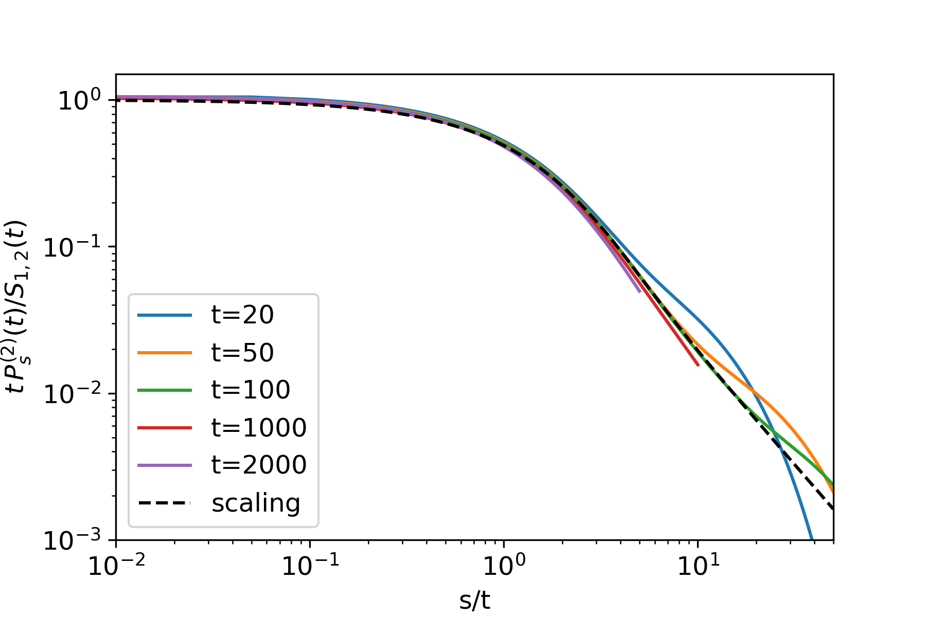
Figure 4. Scaling of the probability $P_{s}^{(2)}(t)$ of finding $s$ type-2 cells at time $t$; different lines indicate different times $t$. Probabilities are calculated numerically from the exact generating function (22) via the Inverse Fast Fourier Transform algorithm, see Appendix C. In the double limit $t,\ s\to\infty$, with $s/t$ constant, the scaled distributions converge to the scaling limit given by (43), depicted by dashed line.

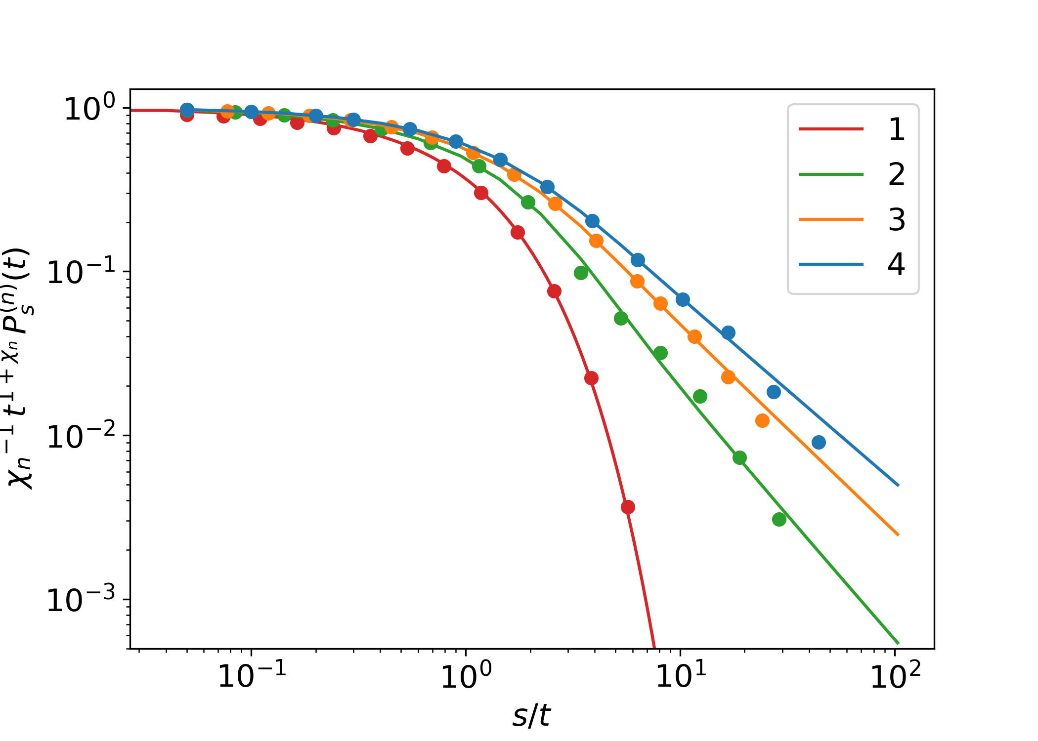
Figure 5. The scaled number distributions $\chi_{n}^{-1}t^{1+\chi_{n}}P^{(n)}_{s}(t)$ from simulations (dots) are compared to the theoretical prediction $F(1+\chi_{n};2;-s/t)$, cf. Eq. (43), as a function of $s/t$, where we fix $t=20$. Curves are for $n=1,2,3,4$. Note the power law decay for $n\geq 2$ as opposed to the exponential decay for the single type case ($n=1$).

5.4. Arrival and exit times

Let us study when new cell types appear and disappear from the system. It is easier to work with the infinite type version of the model for this question, otherwise, we need to assume that the type in question is not greater than $n$. For convenience, we study when type-$n$ cells appear or disappear, but the results are of course valid for any type, not only the last.

For the pure birth-mutation process, the exit time of types is straight-forward. Let

$$E_{n}=\sup\{t\geq 0:Z_{n}(t)>0\}$$

denote the time of extinction of type-$n$ cells. For the birth-mutation process, notice that

$$\{E_{n}>t\}=\{Z_{1}(t)+\dots+Z_{n}(t)>0\}.$$

Hence the distribution of $E_{n}$ when starting from a single type $1$ cell is given by the total survival of the $n$-type process, which we derived asymptotically in (35).

Let us now turn to the arrival time

$$T_{n}=\inf\{t\geq 0:Z_{n}(t)>0\}$$

when the first type-$n$ cell appears. We are interested in its distribution starting with a single type-$i$ cell

$$h_{i,n}(t)=\mathbb{P}(T_{n}>t|Z_{k}(0)=\delta_{ik}).$$

To derive an equation for this quantity consider a modified system where type $n$ cells neither divide nor die, just stay alive forever. Hence their generating function, when starting with a single type $n$ cell, stays constant ${\mathcal{Z}}_{n,n}=x_{n}$, but all other equations for $i<n$ remain the same in (30). The existence of a type $n$ cell in the modified system then indicates that they were produced also in the original system. Hence $h_{i,n}(t)={\mathcal{Z}}_{i,n}(1,\dots,1,0,t)$, and thus

(46) $$\frac{dh_{i,n}}{dt}=h_{i,n}^{2}-2h_{i,n}+h_{i+1,n}$$

with initial condition $h_{i,n}(0)=1$ for $i=1\dots,n-1$ and $h_{n,n}(t)\equiv 0$. In terms of $g_{i,n}(t)=1-h_{i,n}(t)=\mathbb{P}(T_{n}\leq t|Z_{k}(t)=\delta_{ik})$, equation (46) takes a simpler form

(47) $$\frac{dg_{i,n}}{dt}=-g_{i,n}^{2}+g_{i+1,n}$$

with initial condition $g_{i,n}(0)=0$ for $i<n$ and $g_{n,n}(t)\equiv 1$ for all $t$.

For the arrival of the first type-$2$ cell the above equation becomes

(48) $$\frac{dg_{1,2}}{dt}=-g_{1,2}^{2}+1$$

with solution

(49) $$g_{1,2}(t)=\tanh{t}$$

Hence the first type-2 cell arrives on average at

$$\mathbb{E}T_{2}=\log 2.$$

Note also that

(50) $$h_{1,2}(t)=1-g_{1,2}(t)=\mathbb{P}(T_{2}>t|Z_{k}(0)=\delta_{1k})=\frac{2}{1+e^{2t}}$$

have the same form as for the analogous supercritical process [24].

Now we can use this solution for the arrival of type-3 cells, by noting that $g_{i+1,n}=\sigma(g_{i,n-1})$ and we get

(51) $$\frac{dg_{1,3}}{dt}=-g_{1,3}^{2}+\tanh{t}.$$

The solution of (51) can be expressed as a lengthy combination of hypergeometric functions. For subsequent types, no exact solutions are available.

Let us study instead the more general birth-death process described by scheme (2). The above method presented for the birth-mutation process stays valid, and for a constant mutation rate $\nu$ for all types, equation (47) becomes

(52) $$\frac{dg_{i,n}}{dt}=-g_{i,n}^{2}+\nu g_{i+1,n}$$

with initial conditions $g_{i,n}(0)=0$ and $g_{n,n}\equiv 1$. The simplest non-trivial property of this process is

$$g_{1,n}(\infty):=\lim_{t\to\infty}g_{1,n}(t)$$

that is the probability that the first type-$n$ mutant eventually arrives starting from a single type-$1$ cell. For the simple birth-mutation process ($\nu=1$) this quantity is trivial: $g_{1,n}(\infty)=1$ for all $n$, namely all types arrive eventually with probability $1$. This is not the case in the more general birth-death case where, by setting the left-hand side of (52) to zero, we obtain that

$$g_{1,n}(\infty)=\nu^{1-\chi_{n}}.$$

If we denote by $M$ the maximal type that ever appears, then what we found is that $\mathbb{P}(M\geq n)=g_{1,n}(\infty)=\nu^{1-\chi_{n}}$. It gets easier for larger types to appear, in the sense that $\mathbb{P}(M\geq n+1|M\geq n)=\nu^{2^{-n}}\to 1$ as $n\to\infty$. This also implies that the mean number of types that ever appear is infinite, $\mathbb{E}M=\infty$.

Since $g_{2,2}\equiv 1$, we can get an explicit solution for the arrival of the first type-2 cell

$$g_{1,2}(t)=\sqrt{\nu}\tanh\sqrt{\nu}t$$

instead of (49).

For the arrival of the first type-3 cell, using that $g_{2,3}=\sigma(g_{1,2})=g_{1,2}$, we have that

(53) $$\frac{dg_{1,3}}{dt}=-g_{1,3}^{2}+\sqrt{\nu}\tanh\sqrt{\nu}t.$$

The initial condition is $g_{1,3}(0)=0$. Let us normalize $g_{1,3}$ by its limiting probability $g_{1,3}(\infty)=\nu^{3/4}$. That is, we introduce $\tilde{g}_{1,3}:=\tfrac{g_{1,3}}{g_{1,3}(\infty)}$ to get

$$\frac{1}{g_{1,3}(\infty)}\,\frac{d\tilde{g}_{1,3}}{dt}=-\tilde{g}_{1,3}^{2}+\tanh{\sqrt{\nu}t}.$$

Next, we re-scale time, $t\to\tilde{t}=tg_{1,3}(\infty)=t\nu^{3/4}$, and define

$$k_{1,3}(\tilde{t})=\tilde{g}_{1,3}\left(\tilde{t}\nu^{-3/4}\right)=\nu^{-3/4}g_{1,3}(t)$$

to arrive at

$$\frac{dk_{1,3}}{d\tilde{t}}=-k_{1,3}^{2}+\tanh{\nu^{-1/4}\tilde{t}}.$$

In the limit where $\nu\to 0$ we get

$$\frac{dk_{1,3}}{d\tilde{t}}\approx-k_{1,3}^{2}+1,$$

which is the same differential equation we have for $g_{1,2}$ for $\nu=1$ in (48) with the same initial condition $k_{1,3}(0)=0$. Hence $k(\tilde{t})=\tanh\tilde{t}$ and then

$$g_{1,3}(t)\approx\nu^{3/4}\tanh{\nu^{3/4}t}.$$

The same procedure can be applied to obtain the arrival distribution of all types,

(54) $$g_{1,n}\left(t\right)\approx g_{1,n}(\infty)\tanh(g_{1,n}(\infty)t)=\nu^{1-\chi_{n}}\tanh{\nu^{1-\chi_{n}}t}$$

which can be then verified by induction. In Figure 6 we observe that, for a fixed type, the asymptotic agrees with the behaviour in the $\nu\to 0$ limit. However, for a fixed $\nu$, the approximation becomes worse as we consider more types.

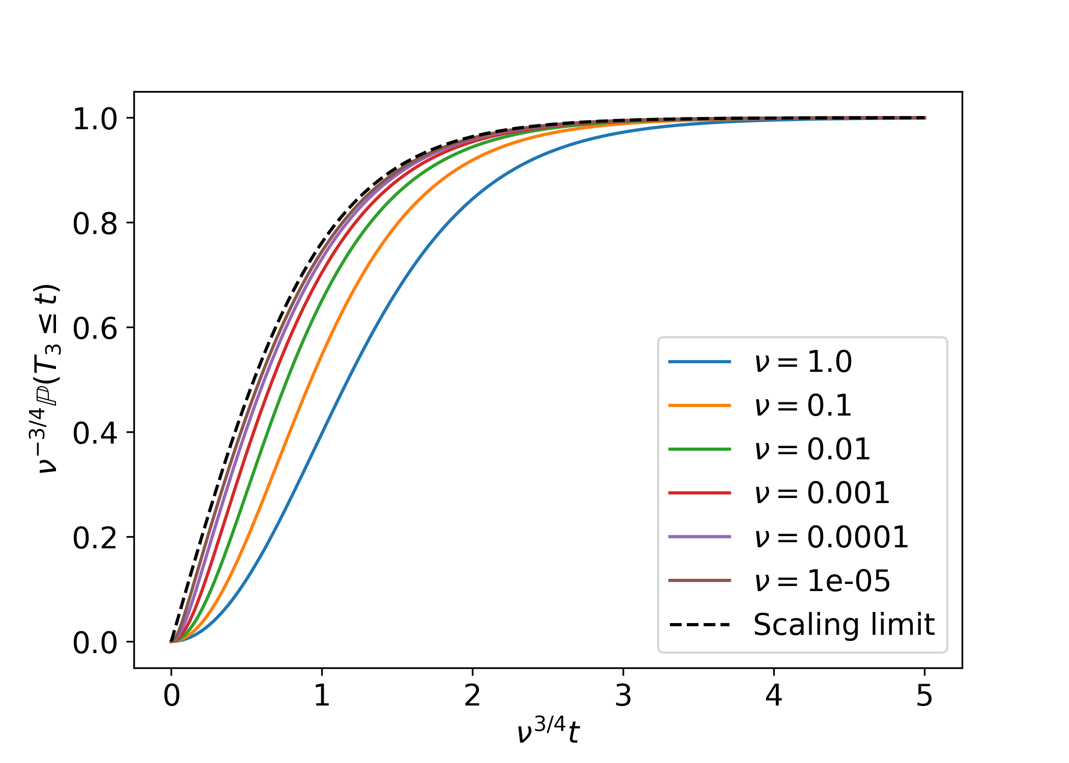
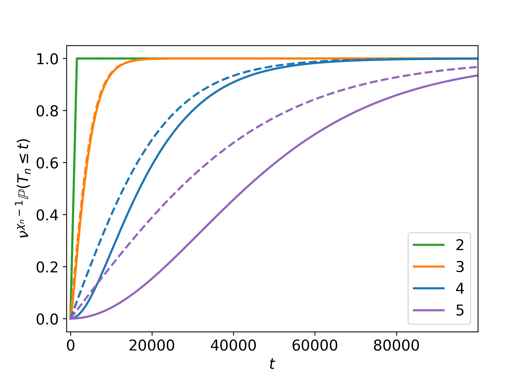
Figure 6. On the left, the scaled probability of arrival of the first type-$3$ cell, $\nu^{-3/4}\mathbb{P}(T_{3}\leq t)$ in terms of $\nu^{3/4}t$, obtained numerically from (52) for different $\nu$ is compared to the scaling limit (54). On the right, the normalized arrival probability $\nu^{\chi_{n}-1}\mathbb{P}(T_{n}\leq t)$ of different types obtained numerically from (52) are compared to the corresponding scaling limit (54) (dashed line) for $\nu=10^{-5}$ and $n=2,\dots,5$.

6. Discussion

Multi-type branching processes provide a natural tool to model biological processes driven by cell division, death, and mutation. Due to their potential to describe evolutionary dynamics, extensive work has been dedicated to deriving solutions of multi-type processes, especially the super-critical and sub-critical cases [13, 24]. In this work, we have focused on finite-type critical processes, which mimic populations in which mutations accumulate until a maximal number of alterations is reached, resulting in extinction.

Driven by biological motivation, we have focused on deriving solutions for the survival of the population, the number of cells, and the arrival and extinction time of cells with different mutations. We found that the survival probability of the overall system, which is asymptotically equivalent to the survival probability of the last type of cells, decays as $t^{-\chi_{n}}$ for the $n$th type. The $\chi_{n}=2^{1-n}$ exponents had been derived by previous work by Foster and Ney [18] and Ogura [25], although following different approaches. With our approach we have also derived higher-order terms, facilitating the estimation of the accuracy of the first-order term.

For two cell types, the generating function of the population sizes was expressed explicitly in terms of modified Bessel functions. This provides a numerically efficient way to extract the number distributions, as detailed in Appendix C. By conditioning on survival (of any cells), we extract the distribution of the number of type-$k$ cells in the large time limit. The survival probabilities show us that the system becomes quickly dominated by the last type of cells, and indeed the distribution of the last type coincides with that of the total number of cells. This distribution only depends on the ratio $s/t$ of the size $s$ of the population and time $t$. Interestingly, in the large $s/t$ limit, this has algebraic and stationary tail $(\text{size})^{-1-\chi_{n}}$. That is, for a fixed (large) number of cells, there is a time regime during which the probability of finding $s$ cells remains constant in time. Since this fat tail – for each but the first cell type – would imply infinite population size, we have derived an upper cutoff for the power law tail which ensures the finiteness of the mean population sizes. These power-law tails appearing for large times for $n\geq 2$ cell types are in sharp contrast to the purely exponential behavior of the mass function of the first cell type. Although the solution is only valid for large time and population size, this corresponds to the range of interest in biological applications.

Throughout this paper, we have focused on the simplest $n$-type critical process, with zero death rate for all but the last cell type. The more general case including cell death, and arbitrary mutation and division rates can be found in Appendix E. This could be relevant for particular applications, to model the effect of accumulating mutations with different division, mutation, and death rates, as long as all cell types have critical growth. Including intermediate types with sub-critical and super-critical growth remains a challenge for future work.

We provide a new mechanism for the error catastrophe: populations of cells that divide and mutate or die at the same rates, and have a maximal number of mutations tolerable. In the context of cancer, this maximal number might represent the amount of DNA damage that can accumulate before being detected by the immune system [29]. We provide exact or asymptotic formulas for our model of the error catastrophe in time, including the evolution of population size, and the time of arrival and extinction of sub-populations. We find that the modeled populations become dominated by cells carrying the maximal number of mutations, and thus loose genetic diversity. This is related to the idea that genetic instability results in extinction because populations cannot overcome selective barriers [35, 2, 36]. Another interesting behaviour is that populations undergoing error catastrophe reach a stationary phase before going extinct. Stationary growth of cancer or bacteria populations is normally associated with having reached a carrying capacity (due to limited nutrients, etc.) [21, 37]. Our model shows that this macroscopic behaviour might be caused by mutational burden, in which case the fate of the population is drastically different, highlighting the importance of considering genetic structure when modeling population growth. As shown in previous work, the applications of multi-type critical processes extend beyond error catastrophe, e.g., to modeling infectious disease spread [5].

Appendix A Two types with general rates

The solution for the two type case has appeared in [4], but we recall the results here for ease of reference with $\alpha_{1}$ explicitly included in the formulas

(55) $$\mathcal{Z}_{1,2}(x_{1},x_{2},t)=1-\frac{\nu_{1}}{\alpha_{2}\tau}\,\frac{I_{0}(2\tau)-cK_{0}(2\tau)}{I_{1}(2\tau)+cK_{1}(2\tau)}$$

where we used the variable

$$\tau=\sqrt{\frac{\nu_{1}}{\alpha_{2}}\left(\frac{\alpha_{1}}{\alpha_{2}(1-x_{2})}+t\alpha_{1}\right)}$$

and the amplitude

(56) $$c=\frac{I_{0}(2\tau_{0})-\alpha_{2}\nu_{1}^{-1}\tau_{0}(1-x_{1})I_{1}(2\tau_{0})}{K_{0}(2\tau_{0})+\alpha_{2}\nu_{1}^{-1}\tau_{0}(1-x_{1})K_{1}(2\tau_{0})}$$

where $\tau_{0}\equiv\tau(t=0)$.

Appendix B Integral formulas $P_{a,b}(t)$

The variable $x_{1}$ appears in (22) only through $c$, while $c$ is a ratio of linear (in variable $x_{1}$) functions. Therefore $\mathcal{Z}_{1,2}$ itself can be transformed into the ratio of linear in $x$ functions. We can expand in $x_{1}$ and effectively we do not need to take the integral in the (complex) $x_{1}$ plane. Thus for $a=0$ we have

(57) $$P_{0,b}(t)=\frac{1}{2\pi i}\oint\frac{dx_{2}}{x_{2}^{b+1}}\,\mathcal{Z}_{1}(0,x_{2},t)$$

while for $a>0$

(58) $$P_{a,b}(t)=\frac{1}{2\pi i}\oint\frac{dx_{2}}{x_{2}^{b+1}}\,\frac{\tau_{0}^{a}}{\tau}\,\frac{(f^{\prime})^{a-1}(fg^{\prime}-f^{\prime}g)}{(f+\tau_{0}f^{\prime})^{a+1}}.$$

Here we used shorthand notation

$$f = I_{1}(2\tau)K_{0}(2\tau_{0})-K_{1}(2\tau)I_{0}(2\tau_{0})$$

$$f^{\prime} = K_{1}(2\tau)I_{1}(2\tau_{0})-I_{1}(2\tau)K_{1}(2\tau_{0})$$

$$g = I_{0}(2\tau)K_{0}(2\tau_{0})-K_{0}(2\tau)I_{0}(2\tau_{0})$$

$$g^{\prime} = K_{0}(2\tau)I_{1}(2\tau_{0})-I_{0}(2\tau)K_{1}(2\tau_{0}).$$

Appendix C Numerical solutions for $P_{a,b}(t)$ and $P_{s}^{(2)}(t)$

Explicit solutions for $P_{a,b}(t)$ are not available. Numerically, however, one can access the probabilities. Using Mathematica’s SeriesCoefficient command we get

$$P_{a,b}(1)\approx\left(\begin{array}[]{ccccc}0.169102&0.190391&0.0789005&0.0341278&\cdots\\ 0.15659&0.0529594&0.0224725&0.00989238&\cdots\\ 0.0692559&0.0298649&0.0138336&0.00643762&\cdots\\ 0.0306302&0.0160577&0.00810575&0.00399019&\cdots\\ \vdots&\vdots&\vdots&\vdots&\end{array}\right)$$

for $a,b=0,1,2,3$, which values can be used to check simulations. Simulating the process (for a few seconds on an average laptop with a code in C) over $10^{8}$ runs we get

$$P_{a,b}(1)\approx\left(\begin{array}[]{ccccc}0.169107&0.190410&0.078873&0.034104&\cdots\\ 0.156639&0.052987&0.022464&0.009880&\cdots\\ 0.069277&0.029886&0.013826&0.006427&\cdots\\ 0.030605&0.016039&0.008102&0.003988&\cdots\\ \vdots&\vdots&\vdots&\vdots&\end{array}\right)$$

However, this approach only works for small $t$. In order to obtain numerical solutions for large $t$, one can invert the generating function via Fourier transform, and apply the Inverse Fast Fourier Transform (IFFT) algorithm as an efficient method to calculate the probability density from the generating function [1]. As an example, we illustrate how to obtain $P_{s}^{(2)}(t)$, that is, the probability of there being $s$ type-2 cells. In order to obtain the joint distribution, one needs to invert Equation (58). Recall the generating function for type-2 cells

$$\mathcal{Z}_{1,2}(1,x,t)=\sum_{s\geq 0}P^{(2)}_{s}(t)x^{s}.$$

The correspondence to the Fourier transform is easier to see if we consider $z=1/x$,

$$\mathcal{Z}_{1,2}(1,1/z,t)=\sum_{s\geq 0}P^{(2)}_{s}(t)z^{-s}$$

this has inversion

(59) $$P^{(2)}_{s}(t)=\frac{1}{2\pi i}\oint_{C}{dz}\,{z^{s-1}}\,\mathcal{Z}_{1}(1,1/z,t)$$

where the contour $C$ goes counterclockwise around the origin in the complex $y$ plane, and must enclose all poles of $\mathcal{Z}_{1}(1,1/z,t)$. We choose $C$ to be a circle of radius $R$ enclosing all poles, and set $z=Re^{i\theta}$,

(60) $$P^{(2)}_{s}(t) =\frac{R^{s}}{2\pi}\int_{0}^{2\pi}{d\theta}\,\mathcal{Z}_{1}(1,Re^{-i\theta},t){e^{i\theta s}}.$$

We notice that we recover a Fourier series expansion. The above integral can be approximated as a sum by splitting the circle into $N$ equidistant discrete points

(61) $${p^{(2)}_{s}(t)}=\frac{R^{s}}{N}\sum_{k=0}^{N-1}\mathcal{Z}_{1}(1,Re^{-2ik\pi/N},t)e^{2isk\pi/N}$$

which is the Inverse Discrete Fourier Transform scaled by $R^{s}$. Thus, we can use the IFFT algorithm to obtain the approximate probability density function. The approximation error of ${p^{(2)}_{s}(t)}\approx P^{(2)}_{s}(t)$ depends on the discretization, and has been largely discussed in the literature [1, 8]. In summary, one can use the following algorithm to extract the probabilities numerically:

1. Calculate $\mathcal{Z}_{1}(1,Re^{-i\theta},t)=\mathcal{Z}_{1}(1,1/z,t),\,z=Re^{i\theta}$.

2. Discretize the circle into $N$ equidistant points.

3. Evaluate the generating function at each point. That is, calculate $\mathcal{Z}_{1}[k]:=\mathcal{Z}_{1}(1,Re^{-2\pi k/N},t)$ for $k=0,\dots,N-1$.

4. Calculate the IDFT of $\mathcal{Z}_{1}[k]$ using Fast Inverse Fourier Transform (e.g. fft.ifft in Numpy or InverseFourierTransform in Mathematica). This outputs $N$ coefficients $q_{0},\dots,q_{N-1}.$

5. Re-scale the $s$th coefficient by $R^{s}$ to recover the probability of $s$ cells,

   $$P^{(2)}_{s}(t)\approx{p^{(2)}_{s}(t)}=R^{s}q_{s}.$$

Note that the generating function of the two-type system $\mathcal{Z}_{1,2}(x_{1},x_{2},t)$ has a singularity at $x_{2}=1$. Thus, we must take $R>1$. From equation (60) we see that the radius $R$ does not affect the inversion. However, numerical errors due to finite precision number representation result in numerical errors with $R$. In Figure 4 we take $R=1.0001$ as we find that if $R$ is increased it becomes difficult to resolve the separate contributions from the poles and zeros of $\mathcal{Z}_{1}(1,1/z,t)$. However, in other settings, numerical problems might arise if $R$ is decreased to too close to the furthest pole. In general, it is common practice to take $R$ to be $10\%$ larger than the largest pole [8].

Appendix D Useful formulas and asymptotic results

We use the large $z$ expansions for the first and second type modified Bessel functions (Section 3.13 of [7], Section 10.7 of [10]),

(62) $$I_{n}(z) \sim\frac{e^{z}}{\sqrt{2\pi z}}\left(1-\frac{4n^{2}-1}{8z}+\frac{(4n^{2}-1)(4n^{2}-9)}{2!(8z)^{2}}-\dots\right),$$

(63) $$K_{n}(z) \sim\sqrt{\frac{\pi}{2z}}e^{-z}\left(1-\frac{4n^{2}-1}{8z}+\frac{(4n^{2}-1)(4n^{2}-9)}{2!(8z)^{2}}-\dots\right).$$

The leading order terms are

$$I_{n}(s)\sim\frac{e^{z}}{\sqrt{2\pi z}}\quad\text{and}\quad K_{n}(z)\sim\sqrt{\frac{\pi}{2z}}e^{-z}.$$

We often use $I_{0}(z)/I_{1}(z)\sim 1$, $K_{1}(z)\sim 0$ and $K_{0}(z)\sim 0$. On some occasions, we are interested in higher-order terms, which can be obtained by considering more terms in the asymptotic expansions. In particular

$$I_{0}(z)/I_{1}(z)=1+\frac{1}{z}+\frac{1}{2z^{2}}+\frac{27}{16z^{3}}+\frac{141}{128z^{4}}+O\left(\left(\frac{1}{z}\right)^{5}\right).$$

Appendix E $n$ types with general rates

Here we generalize our results to the $n$-type process to include death and mutation at arbitrary rates. This is described by the scheme

$$\begin{split}\lx@xy@svg{\hbox{\raise 0.0pt\hbox{\kern 21.88889pt\hbox{\ignorespaces\ignorespaces\ignorespaces\hbox{\vtop{\kern 0.0pt\offinterlineskip\halign{\entry@#!@&&\entry@@#!@\cr&&&\\&&&\\&&&\crcr}}}\ignorespaces{\hbox{\kern-21.88889pt\raise 0.0pt\hbox{\hbox{\kern 0.0pt\raise 0.0pt\hbox{\hbox{\kern 3.0pt\raise 0.0pt\hbox{$\textstyle{(1)+(1)}$}}}}}}}{\hbox{\kern 45.88889pt\raise 0.0pt\hbox{\hbox{\kern 0.0pt\raise 0.0pt\hbox{\hbox{\kern 3.0pt\raise 0.0pt\hbox{$\textstyle{(2)+(2)}$}}}}}}}{\hbox{\kern 117.41666pt\raise 0.0pt\hbox{\hbox{\kern 0.0pt\raise 0.0pt\hbox{\hbox{\kern 3.0pt\raise 0.0pt\hbox{$\textstyle{}$}}}}}}}{\hbox{\kern 151.16666pt\raise 0.0pt\hbox{\hbox{\kern 0.0pt\raise 0.0pt\hbox{\hbox{\kern 3.0pt\raise 0.0pt\hbox{$\textstyle{(n)+(n)}$}}}}}}}{\hbox{\kern-9.3889pt\raise-40.0pt\hbox{\hbox{\kern 0.0pt\raise 0.0pt\hbox{\hbox{\kern 3.0pt\raise 0.0pt\hbox{$\textstyle{(1)\ignorespaces\ignorespaces\ignorespaces\ignorespaces\ignorespaces\ignorespaces\ignorespaces\ignorespaces\ignorespaces\ignorespaces\ignorespaces\ignorespaces}$}}}}}}}\ignorespaces\ignorespaces\ignorespaces\ignorespaces{}{\hbox{\lx@xy@droprule}}\ignorespaces\ignorespaces\ignorespaces{\hbox{\kern 0.0pt\raise-20.0pt\hbox{{}\hbox{\kern 0.0pt\raise 0.0pt\hbox{\hbox{\kern 3.0pt\hbox{\hbox{\kern 0.0pt\raise-0.8625pt\hbox{$\scriptstyle{\alpha_{1}}$}}}\kern 3.0pt}}}}}}\ignorespaces{\hbox{\kern 0.0pt\raise-5.5pt\hbox{\hbox{\kern 0.0pt\raise 0.0pt\hbox{\lx@xy@tip{1}\lx@xy@tip{-1}}}}}}{\hbox{\lx@xy@droprule}}{\hbox{\lx@xy@droprule}}\ignorespaces\ignorespaces\ignorespaces\ignorespaces{}{\hbox{\lx@xy@droprule}}\ignorespaces\ignorespaces\ignorespaces{\hbox{\kern 28.15996pt\raise-45.15138pt\hbox{{}\hbox{\kern 0.0pt\raise 0.0pt\hbox{\hbox{\kern 3.0pt\hbox{\hbox{\kern 0.0pt\raise-0.8625pt\hbox{$\scriptstyle{\nu_{1}}$}}}\kern 3.0pt}}}}}}\ignorespaces{\hbox{\kern 58.38887pt\raise-40.0pt\hbox{\hbox{\kern 0.0pt\raise 0.0pt\hbox{\lx@xy@tip{1}\lx@xy@tip{-1}}}}}}{\hbox{\lx@xy@droprule}}{\hbox{\lx@xy@droprule}}\ignorespaces\ignorespaces\ignorespaces\ignorespaces{}{\hbox{\lx@xy@droprule}}\ignorespaces\ignorespaces\ignorespaces{\hbox{\kern 0.0pt\raise-59.51389pt\hbox{{}\hbox{\kern 0.0pt\raise 0.0pt\hbox{\hbox{\kern 3.0pt\hbox{\hbox{\kern 0.0pt\raise-0.8625pt\hbox{$\scriptstyle{\alpha_{1}-\nu_{1}}$}}}\kern 3.0pt}}}}}}\ignorespaces{\hbox{\kern 0.0pt\raise-68.52777pt\hbox{\hbox{\kern 0.0pt\raise 0.0pt\hbox{\lx@xy@tip{1}\lx@xy@tip{-1}}}}}}{\hbox{\lx@xy@droprule}}{\hbox{\lx@xy@droprule}}{\hbox{\kern 58.38887pt\raise-40.0pt\hbox{\hbox{\kern 0.0pt\raise 0.0pt\hbox{\hbox{\kern 3.0pt\raise 0.0pt\hbox{$\textstyle{(2)\ignorespaces\ignorespaces\ignorespaces\ignorespaces\ignorespaces\ignorespaces\ignorespaces\ignorespaces\ignorespaces\ignorespaces\ignorespaces\ignorespaces}$}}}}}}}\ignorespaces\ignorespaces\ignorespaces\ignorespaces{}{\hbox{\lx@xy@droprule}}\ignorespaces\ignorespaces\ignorespaces{\hbox{\kern 67.77777pt\raise-20.0pt\hbox{{}\hbox{\kern 0.0pt\raise 0.0pt\hbox{\hbox{\kern 3.0pt\hbox{\hbox{\kern 0.0pt\raise-0.8625pt\hbox{$\scriptstyle{\alpha_{2}}$}}}\kern 3.0pt}}}}}}\ignorespaces{\hbox{\kern 67.77777pt\raise-5.5pt\hbox{\hbox{\kern 0.0pt\raise 0.0pt\hbox{\lx@xy@tip{1}\lx@xy@tip{-1}}}}}}{\hbox{\lx@xy@droprule}}{\hbox{\lx@xy@droprule}}\ignorespaces\ignorespaces\ignorespaces\ignorespaces{}{\hbox{\lx@xy@droprule}}\ignorespaces\ignorespaces\ignorespaces{\hbox{\kern 88.36829pt\raise-45.15138pt\hbox{{}\hbox{\kern 0.0pt\raise 0.0pt\hbox{\hbox{\kern 3.0pt\hbox{\hbox{\kern 0.0pt\raise-0.8625pt\hbox{$\scriptstyle{\nu_{2}}$}}}\kern 3.0pt}}}}}}\ignorespaces{\hbox{\kern 113.66666pt\raise-40.0pt\hbox{\hbox{\kern 0.0pt\raise 0.0pt\hbox{\lx@xy@tip{1}\lx@xy@tip{-1}}}}}}{\hbox{\lx@xy@droprule}}{\hbox{\lx@xy@droprule}}\ignorespaces\ignorespaces\ignorespaces\ignorespaces{}{\hbox{\lx@xy@droprule}}\ignorespaces\ignorespaces\ignorespaces{\hbox{\kern 67.77777pt\raise-59.51389pt\hbox{{}\hbox{\kern 0.0pt\raise 0.0pt\hbox{\hbox{\kern 3.0pt\hbox{\hbox{\kern 0.0pt\raise-0.8625pt\hbox{$\scriptstyle{\alpha_{2}-\nu_{2}}$}}}\kern 3.0pt}}}}}}\ignorespaces{\hbox{\kern 67.77777pt\raise-68.52777pt\hbox{\hbox{\kern 0.0pt\raise 0.0pt\hbox{\lx@xy@tip{1}\lx@xy@tip{-1}}}}}}{\hbox{\lx@xy@droprule}}{\hbox{\lx@xy@droprule}}{\hbox{\kern 113.66666pt\raise-40.0pt\hbox{\hbox{\kern 0.0pt\raise 0.0pt\hbox{\hbox{\kern 3.0pt\raise 0.0pt\hbox{$\textstyle{\cdots\ignorespaces\ignorespaces\ignorespaces\ignorespaces}$}}}}}}}\ignorespaces\ignorespaces\ignorespaces\ignorespaces{}{\hbox{\lx@xy@droprule}}\ignorespaces\ignorespaces\ignorespaces{\hbox{\kern 139.64119pt\raise-45.15138pt\hbox{{}\hbox{\kern 0.0pt\raise 0.0pt\hbox{\hbox{\kern 3.0pt\hbox{\hbox{\kern 0.0pt\raise-0.8625pt\hbox{$\scriptstyle{\nu_{n-1}}$}}}\kern 3.0pt}}}}}}\ignorespaces{\hbox{\kern 164.1678pt\raise-40.0pt\hbox{\hbox{\kern 0.0pt\raise 0.0pt\hbox{\lx@xy@tip{1}\lx@xy@tip{-1}}}}}}{\hbox{\lx@xy@droprule}}{\hbox{\lx@xy@droprule}}{\hbox{\kern 164.1678pt\raise-40.0pt\hbox{\hbox{\kern 0.0pt\raise 0.0pt\hbox{\hbox{\kern 3.0pt\raise 0.0pt\hbox{$\textstyle{(n)\ignorespaces\ignorespaces\ignorespaces\ignorespaces\ignorespaces\ignorespaces\ignorespaces\ignorespaces}$}}}}}}}\ignorespaces\ignorespaces\ignorespaces\ignorespaces{}{\hbox{\lx@xy@droprule}}\ignorespaces\ignorespaces\ignorespaces{\hbox{\kern 174.05788pt\raise-20.0pt\hbox{{}\hbox{\kern 0.0pt\raise 0.0pt\hbox{\hbox{\kern 3.0pt\hbox{\hbox{\kern 0.0pt\raise-1.07639pt\hbox{$\scriptstyle{\alpha_{n}}$}}}\kern 3.0pt}}}}}}\ignorespaces{\hbox{\kern 174.05788pt\raise-5.5pt\hbox{\hbox{\kern 0.0pt\raise 0.0pt\hbox{\lx@xy@tip{1}\lx@xy@tip{-1}}}}}}{\hbox{\lx@xy@droprule}}{\hbox{\lx@xy@droprule}}\ignorespaces\ignorespaces\ignorespaces\ignorespaces{}{\hbox{\lx@xy@droprule}}\ignorespaces\ignorespaces\ignorespaces{\hbox{\kern 174.05788pt\raise-59.51389pt\hbox{{}\hbox{\kern 0.0pt\raise 0.0pt\hbox{\hbox{\kern 3.0pt\hbox{\hbox{\kern 0.0pt\raise-1.07639pt\hbox{$\scriptstyle{\alpha_{n}}$}}}\kern 3.0pt}}}}}}\ignorespaces{\hbox{\kern 174.05788pt\raise-68.52777pt\hbox{\hbox{\kern 0.0pt\raise 0.0pt\hbox{\lx@xy@tip{1}\lx@xy@tip{-1}}}}}}{\hbox{\lx@xy@droprule}}{\hbox{\lx@xy@droprule}}{\hbox{\kern-5.5pt\raise-79.02777pt\hbox{\hbox{\kern 0.0pt\raise 0.0pt\hbox{\hbox{\kern 3.0pt\raise 0.0pt\hbox{$\textstyle{\emptyset}$}}}}}}}{\hbox{\kern 62.27777pt\raise-79.02777pt\hbox{\hbox{\kern 0.0pt\raise 0.0pt\hbox{\hbox{\kern 3.0pt\raise 0.0pt\hbox{$\textstyle{\emptyset}$}}}}}}}{\hbox{\kern 117.41666pt\raise-79.02777pt\hbox{\hbox{\kern 0.0pt\raise 0.0pt\hbox{\hbox{\kern 3.0pt\raise 0.0pt\hbox{$\textstyle{}$}}}}}}}{\hbox{\kern 168.55788pt\raise-79.02777pt\hbox{\hbox{\kern 0.0pt\raise 0.0pt\hbox{\hbox{\kern 3.0pt\raise 0.0pt\hbox{$\textstyle{\emptyset}$}}}}}}}\ignorespaces}}}}\ignorespaces\end{split} \textstyle{(1)+(1)} \textstyle{(2)+(2)} \textstyle{(n)+(n)} \textstyle{(1)\ignorespaces\ignorespaces\ignorespaces\ignorespaces\ignorespaces\ignorespaces\ignorespaces\ignorespaces\ignorespaces\ignorespaces\ignorespaces\ignorespaces} \scriptstyle{\alpha_{1}} \scriptstyle{\nu_{1}} \scriptstyle{\alpha_{1}-\nu_{1}} \textstyle{(2)\ignorespaces\ignorespaces\ignorespaces\ignorespaces\ignorespaces\ignorespaces\ignorespaces\ignorespaces\ignorespaces\ignorespaces\ignorespaces\ignorespaces} \scriptstyle{\alpha_{2}} \scriptstyle{\nu_{2}} \scriptstyle{\alpha_{2}-\nu_{2}} \textstyle{\cdots\ignorespaces\ignorespaces\ignorespaces\ignorespaces} \scriptstyle{\nu_{n-1}} \textstyle{(n)\ignorespaces\ignorespaces\ignorespaces\ignorespaces\ignorespaces\ignorespaces\ignorespaces\ignorespaces} \scriptstyle{\alpha_{n}} \scriptstyle{\alpha_{n}} \textstyle{\emptyset} \textstyle{\emptyset} \textstyle{\emptyset} \textstyle{(1)+(1)} \textstyle{(2)+(2)} \textstyle{(n)+(n)} \textstyle{(1)\ignorespaces\ignorespaces\ignorespaces\ignorespaces\ignorespaces\ignorespaces\ignorespaces\ignorespaces\ignorespaces\ignorespaces\ignorespaces\ignorespaces} \scriptstyle{\alpha_{1}} \scriptstyle{\nu_{1}} \scriptstyle{\alpha_{1}-\nu_{1}} \textstyle{(2)\ignorespaces\ignorespaces\ignorespaces\ignorespaces\ignorespaces\ignorespaces\ignorespaces\ignorespaces\ignorespaces\ignorespaces\ignorespaces\ignorespaces} \scriptstyle{\alpha_{2}} \scriptstyle{\nu_{2}} \scriptstyle{\alpha_{2}-\nu_{2}} \textstyle{\cdots\ignorespaces\ignorespaces\ignorespaces\ignorespaces} \scriptstyle{\nu_{n-1}} \textstyle{(n)\ignorespaces\ignorespaces\ignorespaces\ignorespaces\ignorespaces\ignorespaces\ignorespaces\ignorespaces} \scriptstyle{\alpha_{n}} \scriptstyle{\alpha_{n}} \textstyle{\emptyset} \textstyle{\emptyset} \textstyle{\emptyset}$$

Let $\mathcal{Z}_{i,n}(x_{1},x_{2},\dots x_{n},t)$ denote the generating function starting with a single initial type-$i$ cell. The backward Kolmogorov equations read

$$\partial_{t}\mathcal{Z}_{i,n}=\begin{cases}\alpha_{i}\mathcal{Z}_{i,n}^{2}+\alpha_{i}-\nu_{i}+\nu_{i}\mathcal{Z}_{i+1,n}-2\alpha_{i}\mathcal{Z}_{i,n}&\text{for}\quad{i=1,\dots,n-1}\\ \alpha_{n}(\mathcal{Z}_{n,n}^{2}+1-2\mathcal{Z}_{n,n})&\text{for}\quad{i=n}.\end{cases}$$

E.1. Survival probabilities

We solve the system for the survival probabilities $S_{i,n}(t)=1-\mathcal{Z}_{i,n}(0,0,\dots,0,t)$, given by

$$\frac{dS_{i,n}}{dt}=\begin{cases}\nu_{i}S_{i+1,n}-\alpha_{i}{S_{i,n}}^{2}\quad&\text{for}\quad{i=1,\dots,n-1},\\ -\alpha_{n}S_{n,n}^{2}\quad&\text{for}\quad{i=n},\end{cases}$$

with initial conditions $S_{i,n}(0)=1$ for all $i=1,\dots,n$. Following the procedure outlined in Section 5.1 for the no-death case, we derive the survival probability of the $n$-type process

$$S_{1,n}(t)\sim{\prod_{i=1}^{n-1}{\left(\frac{\nu_{i}}{\alpha_{i}}\right)}^{\chi_{i+1}}(\alpha_{n}t+1)^{-\chi_{n}}}$$

where $\chi_{n}=2^{1-n}$. Note that this system is equivalent to the multi-type critical process without death, up to a re-scaling of time. The asymptotic solutions are exact to the same order, but the convergence is slower.

E.2. Generating functions and total number distribution

We now turn to the generating functions. Again, we already know that

$$\mathcal{Z}_{n,n}=1-\frac{1}{\alpha_{n}t+{(1-x_{n})}^{-1}}$$

and we know that for $t\to\infty$, in the leading order $\mathcal{Z}_{i,n}$ only depends on the last type $x_{n}$, and $x_{n}\to 1$ so we may assume that

$$1-\mathcal{Z}_{i,n}=(B_{i}(t+{(1-x_{n})}^{-1}))^{-A_{i}}$$

and perform leading order expansions as usual to recover the coefficients $B_{i}$ and $A_{i}$ for all types. We arrive at the following expression for the leading order asymptotic generating function starting with a single type-1 cell,

$$Z_{1,n}(x_{1},\dots,x_{n},t)\sim 1-{\prod_{i=1}^{n-1}{\left(\frac{\nu_{i}}{\alpha_{i}}\right)}^{\chi_{i+1}}(\alpha_{n}t+{(1-x_{n})}^{-1})^{-\chi_{n}}}.$$

Now we follow the procedure of the no-death case outlined in Section 5.2, use the scaling variables $x_{n}=1-p/\alpha_{n}t$ and $y=s/\alpha_{n}t$ and take the limit $t\to\infty$ with $p$ and $y$ constants, to find

$$\mathbb{E}(x_{n}^{Z_{n}(t)}|Z(t)>0)\to\int_{0}^{\infty}f_{Y_{n}}(y)e^{-py}dy=1-{\left(\frac{p}{p+1}\right)}^{\chi_{n}}.$$

Inverting this Laplace transform we obtain the density of the limit variable

(64) $$f_{Y_{n}}(y)=\chi_{n}F(1+\chi_{n},2,-y).$$

Therefore, the scaling form of the $n$-type distribution is

(65) $$\begin{split}P^{(n)}_{s}(t)&\sim\chi_{n}\frac{S_{1,n}(t)}{t\alpha_{n}}F(1+\chi_{n},2,-s/t\alpha_{n})\\ &\sim{\prod_{i=1}^{n-1}{\left(\frac{\alpha_{i}}{\nu_{i}}\right)}^{\chi_{i+1}}}{\left(\alpha_{n}t\right)}^{\chi_{n}-1}\chi_{n}F(1+\chi_{n},2,-s/t\alpha_{n}).\end{split}$$

Finally, by taking the large argument asymptotic of the confluent hypergeometric function (Appendix D), we obtain the stationary distribution

(66) $$P^{(n)}_{s}(t)\approx\frac{\chi_{n}\alpha_{n}^{\chi_{n}-1}{\prod_{i=1}^{n-1}{\left(\frac{\alpha_{i}}{\nu_{i}}\right)}^{\chi_{i+1}}}}{\Gamma(1-\chi_{n})}\,s^{-1-\chi_{n}}.$$

As seen before, the algebraic stationary tail describes the behaviour up to an upper-cutoff $s^{\star}$ in the number of cells, which we recover by matching the mean $\mathbb{E}Z_{n}(t)$,

(67) $$t\ll s\ll t^{\tfrac{n-1}{1-\chi_{n}}}.$$

E.3. Arrival times

We now consider the arrival times for different birth and mutation rates for each type, $\alpha_{i}$, $\nu_{i}$ (as described by the scheme (2)). The equations for $g_{i,j}$ satisfy

(68) $$\frac{dg_{i,j}}{dt}=-\alpha_{i}g_{i,j}^{2}+\nu_{i}g_{i+1,j}$$

with initial conditions $g_{i,j}(0)=0$ and $g_{j,j}\equiv 1$.

We have that the asymptotic probability of arrival of the $j$th type starting with a single cell is

(69) $$g_{1,j}(\infty):=\lim_{t\to\infty}g_{1,j}(t)={\left(\tfrac{\nu_{1}}{\alpha_{1}}\right)}^{1/2}{\left(\tfrac{\nu_{2}}{\alpha_{2}}\right)}^{1/4}\dots\left(\tfrac{\nu_{j-1}}{\alpha_{j-1}}\right)^{2^{1-j}}=\prod_{i=1}^{j-1}{\left(\tfrac{\nu_{i}}{\alpha_{i}}\right)}^{2^{-i}}.$$

The small $\nu$ limit for arbitrary birth and death rates is the same as for the pure birth-mutation case (54)

$$g_{1,j}\left(t\right)\approx g_{1,j}(\infty)\tanh{g_{1,j}(\infty)t}.$$

but by normalizing and re-scaling time by (69).

References

- [1] Joseph Abate and Ward Whitt. The fourier-series method for inverting transforms of probability distributions. Queueing systems, 10:5–87, 1992.
- [2] Noemi Andor, Carlo C Maley, and Hanlee P Ji. Genomic instability in cancer: teetering on the limit of tolerance. Cancer research, 77(9):2179–2185, 2017.
- [3] Tibor Antal and P L Krapivsky. Exact solution of a two-type branching process: clone size distribution in cell division kinetics. Journal of Statistical Mechanics: Theory and Experiment, 2010(07):P07028, 2010.
- [4] Tibor Antal and P L Krapivsky. Exact solution of a two-type branching process: models of tumor progression. Journal of Statistical Mechanics: Theory and Experiment, 2011(08):P08018, 2011.
- [5] Tibor Antal and P L Krapivsky. Outbreak size distributions in epidemics with multiple stages. Journal of Statistical Mechanics: Theory and Experiment, 2012(07):P07018, 2012.
- [6] K B Athreya and P E Ney. Branching Processes. Dover Publications, 2004.
- [7] Carl M Bender and Steven Orszag. Advanced mathematical methods for scientists and engineers I: Asymptotic methods and perturbation theory, volume 1. Springer Science & Business Media, 1999.
- [8] JK Cavers. On the fast fourier transform inversion of probability generating functions. IMA Journal of Applied Mathematics, 22(3):275–282, 1978.
- [9] V P Chistyakov. Generalization of a theorem for branching processes. Theory of Probability & Its Applications, 4(1):103–106, 1959.
- [10] NIST Digital Library of Mathematical Functions. https://dlmf.nist.gov/, Release 1.1.10 of 2023-06-15. F. W. J. Olver, A. B. Olde Daalhuis, D. W. Lozier, B. I. Schneider, R. F. Boisvert, C. W. Clark, B. R. Miller, B. V. Saunders, H. S. Cohl, and M. A. McClain, eds.
- [11] Esteban Domingo, Julie Sheldon, and Celia Perales. Viral quasispecies evolution. Microbiology and Molecular Biology Reviews, 76(2):159–216, 2012.
- [12] Rick Durrett. Population genetics of neutral mutations in exponentially growing cancer cell populations. Ann. Appl. Probab., 23(1):230–250, 02 2013.
- [13] Rick Durrett. Branching Process Models of Cancer. Stochastics in Biological Systems. Springer, 2015.
- [14] Manfred Eigen. Error catastrophe and antiviral strategy. Proceedings of the National Academy of Sciences, 99(21):13374–13376, 2002.
- [15] Manfred Eigen, John McCaskill, and Peter Schuster. Molecular quasi-species. The Journal of Physical Chemistry, 92(24):6881–6891, 1988.
- [16] Manfred Eigen and Peter Schuster. The hypercycle: A principle of natural self-organization part b: The abstract hypercycle. Naturwissenschaften, 65:7–41, 1978.
- [17] Robert Fast, Thomas H Eberhard, Tarmo Ruusala, and CG Kurland. Does streptomycin cause an error catastrophe? Biochimie, 69(2):131–136, 1987.
- [18] James Foster and Peter Ney. Decomposable critical multi-type branching processes. Sankhyā: The Indian Journal of Statistics, Series A (1961-2002), 38(1):28–37, 1976.
- [19] James Foster and Peter Ney. Limit laws for decomposable critical branching processes. Zeitschrift für Wahrscheinlichkeitstheorie und Verwandte Gebiete, 46(1):13–43, 1978.
- [20] Edward J Fox and Lawrence A Loeb. Lethal mutagenesis: targeting the mutator phenotype in cancer. In Seminars in cancer biology, volume 20, pages 353–359. Elsevier, 2010.
- [21] Philip Gerlee. The model muddle: in search of tumor growth laws. Cancer research, 73(8):2407–2411, 2013.
- [22] Siân Jones, Wei-dong Chen, Giovanni Parmigiani, Frank Diehl, Niko Beerenwinkel, Tibor Antal, Arne Traulsen, Martin A. Nowak, Christopher Siegel, Victor E. Velculescu, Kenneth W. Kinzler, Bert Vogelstein, Joseph Willis, and Sanford D. Markowitz. Comparative lesion sequencing provides insights into tumor evolution. Proceedings of the National Academy of Sciences, 105(11):4283–4288, 2008.
- [23] Thomas W Mullikin. Limiting distributions for critical multitype branching processes with discrete time. Transactions of the American Mathematical Society, 106(3):469–494, 1963.
- [24] Michael D Nicholson, David Cheek, and Tibor Antal. Mutation accumulation in exponentially growing populations. arXiv preprint arXiv:2208.02088, 2022.
- [25] Yukio Ogura. Asymptotic behavior of multitype galton-watson processes. J. Math. Kyoto Univ, 15(2):251–302, 1975.
- [26] Abe Pressman, Celia Blanco, and Irene A Chen. The rna world as a model system to study the origin of life. Current Biology, 25(19):R953–R963, 2015.
- [27] Sudha Rajamani, Justin K Ichida, Tibor Antal, Douglas A Treco, Kevin Leu, Martin A Nowak, Jack W Szostak, and Irene A Chen. Effect of stalling after mismatches on the error catastrophe in nonenzymatic nucleic acid replication. Journal of the American Chemical Society, 132(16):5880–5885, 2010.
- [28] Josep Sardanyés and Tomás Alarcón. Noise-induced bistability in the fate of cancer phenotypic quasispecies: a bit-strings approach. Scientific reports, 8(1):1–11, 2018.
- [29] Ton N Schumacher and Robert D Schreiber. Neoantigens in cancer immunotherapy. Science, 348(6230):69–74, 2015.
- [30] Boris Alexandrovich Sevast’yanov. Transient phenomena in branching stochastic processes. Theory of Probability & Its Applications, 4(2):113–128, 1959.
- [31] Ricard V Solé and Thomas S Deisboeck. An error catastrophe in cancer? Journal of Theoretical Biology, 228(1):47–54, 2004.
- [32] Ignacio Soriano, Enrique Vazquez, Nagore De Leon, Sibyl Bertrand, Ellen Heitzer, Sophia Toumazou, Zhihan Bo, Claire Palles, Chen-Chun Pai, Timothy C Humphrey, et al. Expression of the cancer-associated dna polymerase p286r in fission yeast leads to translesion synthesis polymerase dependent hypermutation and defective dna replication. PLoS genetics, 17(7):e1009526, 2021.
- [33] Jesse Summers and Samuel Litwin. Examining the theory of error catastrophe. Journal of virology, 80(1):20–26, 2006.
- [34] Jörg Swetina and Peter Schuster. Self-replication with errors: A model for polvnucleotide replication. Biophysical chemistry, 16(4):329–345, 1982.
- [35] Héctor Tejero, Francisco Montero, and Juan Carlos Nuño. Theories of lethal mutagenesis: from error catastrophe to lethal defection. Quasispecies: From Theory to Experimental Systems, pages 161–179, 2016.
- [36] Susanne Tilk, Svyatoslav Tkachenko, Christina Curtis, Dmitri A Petrov, and Christopher D McFarland. Most cancers carry a substantial deleterious load due to hill-robertson interference. Elife, 11:e67790, 2022.
- [37] Kathleen MC Tjørve and Even Tjørve. The use of gompertz models in growth analyses, and new gompertz-model approach: An addition to the unified-richards family. PloS one, 12(6):e0178691, 2017.
- [38] Marco Vignuzzi, Jeffrey K Stone, and Raul Andino. Ribavirin and lethal mutagenesis of poliovirus: molecular mechanisms, resistance and biological implications. Virus research, 107(2):173–181, 2005.
- [39] Shinichi Yachida, Siân Jones, Ivana Bozic, Tibor Antal, Rebecca Leary, Baojin Fu, Mihoko Kamiyama, Ralph H Hruban, James R Eshleman, Martin A Nowak, Victor E Velculescu, Kenneth W Kinzler, Bert Vogelstein, and Christine A Iacobuzio-Donahue. Distant metastasis occurs late during the genetic evolution of pancreatic cancer. Nature, 467(7319):1114–1117, 2010.