Deep Level-set Method for Stefan Problems

Abstract

We propose a level-set approach to characterize the region occupied by the solid in Stefan problems with and without surface tension, based on their recent probabilistic reformulation. The level-set function is parameterized by a feed-forward neural network, whose parameters are trained using the probabilistic formulation of the Stefan growth condition. The algorithm can handle Stefan problems where the liquid is supercooled and can capture surface tension effects through the simulation of particles along the moving boundary together with an efficient approximation of the mean curvature. We demonstrate the effectiveness of the method on a variety of examples with and without radial symmetry.

Keywords: level-set method, mushy region, neural networks, probabilistic solutions, Stefan problem, supercooling, surface tension

Mathematics Subject Classification: 35R35, 68T07, 65K15

1 Introduction

The Stefan problem [21, 40, 41, 42, 43] is central to partial differential equations involving free boundaries. It aims to capture the moving interface separating a solid from a liquid region, as well as the evolution of the temperature in both regions. Despite its simple description and many deep results obtained since its introduction (see, e.g., [13] and the references therein), many intriguing questions remain open. In particular, weak solutions to the Stefan problem are non-unique in general, while strong solutions may fail to exist. Thus, further restrictions are needed to obtain a unique characterization. A recent approach developed by Delarue, Guo, Nadtochiy and the first author [12, 26, 15] provides stochastic representations and proposes the notion of physical probabilistic solutions as a selection principle. This new notion is expected to lie between weak and strong solutions, as shown in [26] for the one-phase supercooled Stefan problem.

Probabilistic solutions satisfy a growth condition relating the change in volume of the solid region, denoted by $\Gamma_{t}$, to the proportion of absorbed “heat” particles in the two phases:

$$\underbrace{|\Gamma_{0}|-|\Gamma_{t}|}_{\text{Volume change of the solid}}=\;\underbrace{\eta\operatorname{\mathbb{P}}(\tau^{1}\leq t)-\operatorname{\mathbb{P}}(\tau^{2}\leq t)}_{\text{Absorbed liquid $\&$ solid heat particles}},$$ (1)

where $\tau^{1}$ (resp. $\tau^{2}$) stands for the hitting time of the moving interface $\partial\Gamma=(\partial\Gamma_{t})_{t\in[0,T]}$ for particles in the liquid (resp. solid). The binary parameter $\eta$ captures the effect of particles in the liquid when the latter has a nonnegative temperature ($\eta=1$) or is supercooled ($\eta=-1$). An exact statement is given in Definitions 1 and 2, below. While probabilistic solutions of the Stefan problem are quite well understood in one space dimension [12, 10] and for radially symmetric solids [15, 25], less is known in the general case. Additional challenges arise when incorporating surface tension effects through the classical Gibbs-Thomson law, [2, 25, 31], which postulates that the temperature at the interface is below (resp. above) the equilibrium melting point where the solid is locally convex (resp. concave).

We leverage the probabilistic solutions of Stefan problems, the celebrated level-set method of Osher and Sethian [27], and the recent advances in training neural networks in order to produce efficient numerical algorithms. More specifically, we represent $\Gamma=(\Gamma_{t})_{t\in[0,T]}$, the evolving region occupied by the solid, by a level-set function which is parameterized by a feed-forward neural network. That is, the evolving solid is given by the zero sublevel set of an appropriate function $\Phi\mathrel{\mathop{\ordinarycolon}}[0,T]\times\operatorname{\mathbb{R}}^{d}\to\operatorname{\mathbb{R}}$, focusing on $d\in\{2,3\}$ in our numerical experiments. The level-set method is widely used to describe the evolution of moving interfaces in arbitrary dimensions as it imposes no assumptions on the geometry of the unknown region and can easily handle changes in topological properties. For example, level sets are able to capture the separation of a connected set into several components and vice versa. As demonstrated in the numerical examples below (Section 4.2.4), this flexibility is of crucial importance for general Stefan problems. We refer the reader to the excellent books by Osher and Fedkiw [28] and Sethian [35] for a comprehensive description of level-set methods.

To the best of our knowledge, the use of the level-set method for the Stefan problem was first proposed in [9]. Their algorithm alternately approximates the moving interface through level-set functions and the temperature in the two phases via a finite difference scheme for the heat equation. The method is capable of accurately reproducing known solutions to the Stefan problem, as well as of generating realistic dendritic growth for a variety of solids (see also [14], focusing on dendritic crystallization, and [28, Section 23], presenting applications to general heat flows). Herein, the level-set function is parameterized by a time-space feedforward neural network $\Phi\mathrel{\mathop{\ordinarycolon}}[0,T]\times\operatorname{\mathbb{R}}^{d}\times\Theta\to\operatorname{\mathbb{R}}$ where $\Theta$ is a finite-dimensional parameter set. The parameters are trained using stochastic gradient descent by converting the growth condition of probabilistic solutions into a loss function. The computation of the latter involves the simulation of reflected Brownian particles in the two phases. The proposed method has the advantage that the normal vector to the interface – which is essential in level-set methods – can be effortlessly computed through automatic differentiation of the deep level-set function.

The training of neural network parameters is achieved by minimizing a loss function that involves stopped particles. Since the hitting times of sharp interfaces lead to vanishing gradient issues and prevent the training of the deep level-set function, we use a relaxation procedure as in [33, 34, 39], developed for optimal stopping. This relaxation consists of introducing a mushy region separating the solid and the liquid as in phase-field models [5, 8, 38], and then using stopping probabilities. The loss function defined in (13), below, tries to enforce the local version (4) of (1) for a large number of randomly chosen test functions. Such a construction based on an identity holding for a class of test functions is novel and may find other applications.

The trained network encapsulates the two phases, and it is important to emphasize that the temperature function does not need to be approximated during training. Due to the probabilistic nature of the algorithm, the temperature function can be estimated later through the empirical measure of the surviving particles. Moreover, surface tension effects can be seamlessly integrated into the algorithm, see Section 3.5. We refer the interested reader to [31] surveying computational methods for differential equations with surface tension in fluid mechanics.

Combining the level-set method with deep learning to solve free boundary problems appears to be new, although our work shares some similarities with [1], which provides a numerical resolution of controlled front propagation flows with the level-set method, and where the velocity is approximated by neural networks and not the level-set function. The present approach is motivated by the recent advances of deep learning to solve complex and/or high-dimensional problems in partial differential equations [18, 36, 45, 30], optimal stopping [6, 7, 33, 34], as well as general stochastic control problems [4, 17, 33]. In the case of physical phenomena, physics-informed neural networks [32, 45] successfully combine observed data with known physical laws to learn the solution for a variety of problems in physics. The neural parameterization of level-set functions has already shown promising results in computer vision. Among others, a neural network is trained to approximate the signed distance function associated with three-dimensional objects in [29] and their occupancy probability in [23].

We believe that the proposed deep level-set method can be applied to problems in a variety of contexts. This includes free boundary problems in physics, such as Hele-Shaw and Stokes flows [11]. In mathematical finance, the method can be used to generalize the neural optimal stopping boundary method of [34] for the exercise boundary of American options with known geometric structure. Also, optimal portfolio problems with transaction costs [24] could benefit from our method once the so-called no-trade zone is represented by a deep level-set function.

Structure of the paper. We introduce the Stefan problem and its probabilistic solution in Section 2. The deep level-set method is described in Section 3 and extended in Section 3.5 for the Stefan problem with surface tension. Section 4 is devoted to the numerical results in the radially symmetric case (Section 4.1) and for general shapes of the solid (Section 4.2). Section 5 concludes, and Appendix A contains the proofs of the main results.

Notations. Given a Lebesgue measurable set $A\subset\operatorname{\mathbb{R}}^{d}$, $d\geq 1$, and a measurable function $\psi\mathrel{\mathop{\ordinarycolon}}\operatorname{\mathbb{R}}^{d}\to\operatorname{\mathbb{R}}$, we employ the shorthand notations $\int_{A}\psi=\int_{A}\psi(x)\,\mathrm{d}x$ and $\int_{\partial A}\psi=\int_{\partial A}\psi(x)\,\mathrm{d}\operatorname{\mathcal{H}}^{d-1}(x)$, where $\operatorname{\mathcal{H}}^{d-1}$ is the $(d-1)$-dimensional Hausdorff measure. We also write $|A|$ for the Lebesgue measure of $A$.

2 Stefan Problems and Probabilistic Solutions

Let $\Omega$ be a bounded domain in $\operatorname{\mathbb{R}}^{d}$, $d\geq 1$, and $T\in(0,\infty)$. Given a closed subset $\Gamma_{0-}\subseteq\overline{\Omega}$ and $u_{0}^{1}\mathrel{\mathop{\ordinarycolon}}\overline{\Omega\setminus\Gamma_{0-}}\to\operatorname{\mathbb{R}},\ u_{0}^{2}\mathrel{\mathop{\ordinarycolon}}\Gamma_{0-}\to\operatorname{\mathbb{R}}_{-}$, the strong formulation of the two-phase Stefan problem amounts to finding a triplet $(u^{1},u^{2},\Gamma)=(u^{1}(t,\cdot),u^{2}(t,\cdot),\Gamma_{t})_{t\in[0,T]}$ such that

$$\partial_{t}u^{i}=\frac{\alpha_{i}}{2}\Delta u^{i}, \Gamma^{i}\mathrel{\mathop{\ordinarycolon}}=\{(t,x)\in(0,T]\times\Omega\mathrel{\mathop{\ordinarycolon}}\,x\in\text{int}\ \Gamma^{i}_{t}\},\;i=1,2,$$ on   int (2a)

$$u^{i}(0-,\cdot)=u^{i}_{0}, \Gamma^{i}_{0-},\;i=1,2,$$ on   (2b)

$$\partial_{\mathfrak{n}}u^{i}=0, \ \partial\Omega\cap\Gamma^{i}\mathrel{\mathop{\ordinarycolon}}=\{(t,x)\in[0,T]\times\partial\Omega\ \mathrel{\mathop{\ordinarycolon}}\ x\in\Gamma^{i}_{t}\},\;i=1,2,$$ on (2c)

$$V=\frac{\alpha_{2}}{2L}\partial_{\nu}u^{2}-\frac{\alpha_{1}}{2L}\partial_{\nu}u^{1}, \partial\Gamma\mathrel{\mathop{\ordinarycolon}}=\{(t,x)\in[0,T]\times\Omega\ \mathrel{\mathop{\ordinarycolon}}\ x\in\partial\Gamma_{t}\},$$ on   (2d)

$$u^{1}=u^{2}=0, \partial\Gamma,$$ on (2e)

where $\Gamma^{1}_{t}=\Omega\setminus\Gamma_{t}$, $\Gamma^{2}_{t}=\Gamma_{t}$ represent respectively the liquid and the solid region, and $\mathfrak{n}$ is the outward normal vector field on $\partial\Omega$. In (2d), $V$ is the outward normal velocity of $\partial\Gamma_{t}$, $\nu$ the outward normal vector field on $\partial\Gamma_{t}$, $L$ the latent heat of fusion, and $\alpha_{1},\alpha_{2}$ the thermal diffusivities. An illustration of the two-phase Stefan problem is given in Fig. 1. We suppose that the boundary $\partial\Gamma_{t}$ is in the solid region so that $\Gamma_{t}^{1}$ (resp. $\Gamma_{t}=\Gamma_{t}^{2}$) is relatively open (resp. closed) in $\Omega$.

The initial temperature in the solid $u_{0}^{2}$ is always assumed to be non-positive. At the same time, the temperature in the liquid $u_{0}^{1}$ is assumed to be either non-negative or non-positive everywhere. For convenience, we introduce the parameter $\eta\mathrel{\mathop{\ordinarycolon}}=\text{sign}(u_{0}^{1})$ which indicates whether the liquid is initially regular ($\eta=1$) or supercooled ($\eta=-1$).

Figure 1: Illustration of the two-phase Stefan problem (2a)-(2e). Evolution of the liquid region (blue) and solid region (white) in a freezing regime for some time points $0\leq s<t\leq T$.

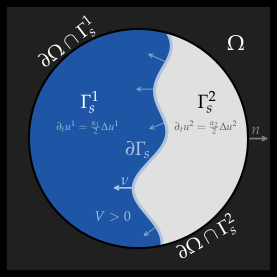
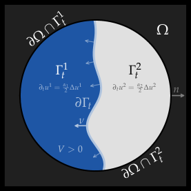
2.1 Probabilistic Solutions

We assume throughout that $\lVert u_{0}^{i}\rVert_{L^{1}(\Gamma_{0-}^{i})}=1,$ $i=1,2$. This requirement can be easily removed, see Remark 2 below. Further, we let $X^{i}$ be a Brownian motion with diffusivity $\alpha_{i}$ that is normally reflected along $\partial\Omega$ and absorbed when hitting the moving interface $\partial\Gamma$ (in light of (2a), (2c), (2e)). More specifically,

$$X_{t}^{i}=X_{0}^{i}+\sqrt{\alpha_{i}}\ W_{t\wedge\tau^{i}}^{i}+l_{t\wedge\tau^{i}}^{i},\;0\leq t\leq T,\quad\tau^{i}=\inf\{t\in[0,T]\mathrel{\mathop{\ordinarycolon}}\,X_{0}^{i}+\sqrt{\alpha_{i}}\ W_{t}^{i}+l_{t}^{i}\notin\Gamma_{t}^{i}\},$$ (3)

where $W^{i}$ is a standard Brownian motion in $\operatorname{\mathbb{R}}^{d}$ and $l^{i}$ the local time process at $\partial\Omega$. In addition, we take $X_{0}^{i}\sim|u_{0}^{i}|(x)\,\mathrm{d}x$. We can now state the definition of a probabilistic solution.

Definition 1.

We say that $(\mu^{1},\mu^{2},\Gamma)$ is a probabilistic solution of the Stefan problem (2a) $\!-$(2e) if for all $t\in[0,T]$, one has

$$\int_{\Gamma_{0-}}\psi-\int_{\Gamma_{t}}\psi=\frac{1}{L}\big{(}\eta\operatorname{\mathbb{E}}^{\mu^{1}}[\psi(X_{\tau^{1}}^{1})\,\mathds{1}_{\{\tau^{1}\leq t\}}]-\operatorname{\mathbb{E}}^{\mu^{2}}[\psi(X_{\tau^{2}}^{2})\,\mathds{1}_{\{\tau^{2}\leq t\}}]\big{)},\quad\psi\in\mathcal{C}^{\infty}_{c}(\Omega),$$ (4)

where $\mu^{i}$ is the law of $X^{i}$, $i=1,2$.

We next prove that the definition of a probabilistic solution is consistent with that of a classical one, as already shown for the one-phase problem in [26, Proposition 5.5].

Proposition 1.

Suppose that $(u^{1},u^{2},\Gamma)$ is a classical solution of the Stefan problem (2a) $\!-$(2e). Let $X^{i}$ be as in (3) and set $\mu^{i}=\operatorname{\mathbb{P}}\circ(X^{i})^{-1}$. Then, $(\mu^{1},\mu^{2},\Gamma)$ is a probabilistic solution of (2a) $\!-$(2e).

Proof.

See Section A.1. ∎

In the course of the proof of Proposition 1, we find that

$$|u^{i}|(t,x)\,\mathrm{d}x=\operatorname{\mathbb{P}}(X_{t}^{i}\in\mathrm{d}x,\,\tau^{i}>t),\quad i=1,2.$$ (5)

The temperature, albeit not our primary focus, can thus be retrieved from the (sub)density of “survived” particles (i.e., those not yet absorbed by the moving boundary $\partial\Gamma$) once $\Gamma=(\Gamma_{t})_{t\in[0,T]}$ has been estimated. Further details are given in Section 4.1.2.

Remark 1.

Suppose that the boundary of the ice region lies entirely in $\Omega$ for all $t\in[0,T]$. Then, a direct approximation argument shows that (4) holds also for smooth test functions which are not compactly supported in $\Omega$, and we may choose $\psi\equiv 1$ to obtain

$$|\Gamma_{0-}|-|\Gamma_{t}|=\;\eta\operatorname{\mathbb{P}}(\tau^{1}\leq t)-\operatorname{\mathbb{P}}(\tau^{2}\leq t).$$

The above identity relates the change in volume of the solid region on the left-hand side to the exit probabilities of liquid and solid particles from their respective regions on the right-hand side, and can be interpreted as energy conservation.

Remark 2.

Suppose that $(u^{1},u^{2},\Gamma)$ is a classical solution of (2a) $\!-$(2e) with initial temperature functions $u_{0}^{i}$ such that $\lVert u_{0}^{i}\rVert_{L^{1}(\Gamma_{0-}^{i})}=c_{i}\in(0,\infty)$, $i=1,2$. After a simple adaptation of the proof of Proposition 1, the growth condition (4) becomes

$$\int_{\Gamma_{0-}}\psi-\int_{\Gamma_{t}}\psi=\frac{1}{L}\big{(}\eta\ c_{1}\operatorname{\mathbb{E}}^{\mu^{1}}[\psi(X_{\tau^{1}}^{1})\,\mathds{1}_{\{\tau^{1}\leq t\}}]-c_{2}\operatorname{\mathbb{E}}^{\mu^{2}}[\psi(X_{\tau^{2}}^{2})\,\mathds{1}_{\{\tau^{2}\leq t\}}]\big{)},\quad\psi\in\mathcal{C}_{c}^{\infty}(\Omega).$$ (6)

The additional flexibility in the initial temperature when $c_{i}\neq 1$ proves useful in the numerical experiments (see Sections 4.1.2 and 4.1.3).

Example 1.

The one-phase Stefan problem consists of setting $u^{2}(t,x)\equiv 0$ in the solid region. If the liquid temperature is initially positive, then the solid is necessarily melting, i.e.: $\Gamma_{t}\subseteq\Gamma_{s}\subseteq\Gamma_{0-}$ for all $0\leq s\leq t\leq T$. Writing $X=X^{1}$, $\tau=\tau^{1}$, and $\mu=\mu^{1}$, the growth condition (4) simply reads

$$\int_{\Gamma_{0-}\setminus\Gamma_{t}}\psi=\frac{\eta}{L}\operatorname{\mathbb{E}}^{\mu}[\psi(X_{\tau})\,\mathds{1}_{\{\tau\leq t\}}],\quad\psi\in\mathcal{C}_{c}^{\infty}(\Omega).$$ (7)

2.2 Adding Surface Tension

Consider the Stefan problem $\eqref{eq:2SPHeat}-\eqref{eq:2SPDirichlet}$ with the Dirichlet boundary condition (2e) replaced by

$$u^{1}=u^{2}=-\gamma\ \kappa_{\partial\Gamma},\quad\text{on }\ \partial\Gamma.$$ (2e’)

The term $\kappa_{\partial\Gamma_{t}}$ is the mean curvature of $\partial\Gamma_{t}$ and $\gamma>0$ the surface tension coefficient. We use the convention that $\kappa_{\partial\Gamma_{t}}(x)$ is nonnegative when $\Gamma_{t}$ is locally convex at $x\in\partial\Gamma_{t}$. Equation (2e’) captures the so-called Gibbs-Thomson effect which postulates that the temperature at the interface is negative for strictly convex boundaries [44, 22]. In other words, the freezing point of the liquid decreases at points of convexity and increases at points of concavity. Clearly, surface tension effects only appear if $d\geq 2$. We now revisit Definition 1 in the presence of surface tension.

Definition 2.

We say that $(\mu^{1},\mu^{2},\Gamma)$ is a probabilistic solution of the Stefan problem (2a) $\!-$(2e’) with surface tension if for all $t\in[0,T]$, one has

$$\int_{\Gamma_{0-}}\psi-\int_{\Gamma_{t}}\psi=\frac{1}{L}\big{(}\eta\operatorname{\mathbb{E}}^{\mu^{1}}[\psi(X_{\tau^{1}}^{1})\,\mathds{1}_{\{\tau^{1}\leq t\}}]-\operatorname{\mathbb{E}}^{\mu^{2}}[\psi(X_{\tau^{2}}^{2})\,\mathds{1}_{\{\tau^{2}\leq t\}}]+\operatorname{\mathcal{K}}_{t}\big{)},\quad\text{where}$$ (8)

$$\operatorname{\mathcal{K}}_{t}=\gamma\int_{0}^{t}\int_{\partial\Gamma_{s}}\left(\frac{\alpha_{2}}{2}\partial_{\nu}K^{2}-\frac{\alpha_{1}}{2}\partial_{\nu}K^{1}\right)\psi\ ,$$ (9)

$$K^{i}(t,x)=\operatorname{\mathbb{E}}\big{[}\kappa_{\!\partial\Gamma_{\overleftarrow{\;\tau}^{i}_{t}}}(X^{i}_{\overleftarrow{\;\tau}^{i}_{t}})\,\mathds{1}_{\{\overleftarrow{\;\tau}^{i}_{t}\leq t\}}\ \big{|}\ X^{i}_{0}=x\big{]},$$ (10)

with the backward exit times $\overleftarrow{\;\tau}^{i}_{t}=\inf\{s\in[0,t]\mathrel{\mathop{\ordinarycolon}}\,X_{0}^{i}+\sqrt{\alpha_{i}}\ W^{i}_{s}+l^{i}_{s}\notin\Gamma^{i}_{t-s}\}$.

Proposition 2.

Suppose that $(u^{1},u^{2},\Gamma)$ is a classical solution of the Stefan problem with surface tension (2a) $\!-$(2e’). If $\mu^{i}\mathrel{\mathop{\ordinarycolon}}=\operatorname{\mathbb{P}}\circ(X^{i})^{-1}$ with $X^{i}$ as in (3), then $(\mu^{1},\mu^{2},\Gamma)$ is a probabilistic solution of (2a)$\!-$(2e’).

Proof.

See Section A.2. ∎

3 Deep Level-set Method

Let $\Gamma=(\Gamma_{t})_{t\in[0,T]}$ be the time-varying region occupied by the solid, and let $\Phi\!\mathrel{\mathop{\ordinarycolon}}[0,T]\times\Omega\to\operatorname{\mathbb{R}}$ be a level-set function such that

$$\Gamma_{t}=\{x\in\Omega\mathrel{\mathop{\ordinarycolon}}\,\Phi(t,x)\leq 0\}$$

and the free boundary $\partial\Gamma_{t}$ is given by the zero isocontour $\{\Phi(t,\cdot)=0\}$. We also assume that the initial region $\Gamma_{0-}$ is encoded as the zero sublevel set of some function $\Phi_{0}\!\mathrel{\mathop{\ordinarycolon}}\Omega\to\operatorname{\mathbb{R}}$. Whenever $\Phi\in\operatorname{\mathcal{C}}^{1,2}([0,T]\times\Omega)$ and $\nabla_{x}\Phi\neq 0$, the normal velocity, outward normal vector, and mean curvature of $\partial\Gamma$ read

$$V=-\frac{\partial_{t}\Phi}{|\nabla_{x}\Phi|},\quad\nu=\frac{\nabla_{x}\Phi}{|\nabla_{x}\Phi|},\quad\kappa_{\partial\Gamma}=\frac{\text{div}(\nu)}{d-1}.$$

In particular, the Stefan condition (2d) can be rewritten as

$$\partial_{t}\Phi=\frac{\alpha_{1}}{2L}\nabla_{x}\Phi\cdot\nabla_{x}u^{1}-\frac{\alpha_{2}}{2L}\nabla_{x}\Phi\cdot\nabla_{x}u^{2}.$$

The signed distance function defined by

$$\rho(t,x)=(-1)^{\mathds{1}_{\Gamma_{t}}}\ dist(x,\partial\Gamma_{t})$$

can always be used as a level-set function and encodes all geometric properties of the interface; see [3, 37] and [28, Section I.2]. In particular, suppose that $\partial\Gamma_{t}$ is a smooth manifold. Then, $\rho$ is differentiable in a neighborhood of $\partial\Gamma_{t}$ and satisfies

$$|\nabla_{x}\rho|=1,\quad V=-\partial_{t}\rho,\quad\nu=\nabla_{x}\rho,\quad\kappa_{\partial\Gamma}=\frac{\Delta_{x}\rho}{d-1},\qquad\text{on }\ \partial\Gamma_{t}.$$

To approximate a general level-set function $\Phi$, we parameterize the difference $\Phi(t,\cdot)-\Phi_{0}$ by a neural network $G\!\mathrel{\mathop{\ordinarycolon}}[0,T]\times\Omega\times\Theta\to\operatorname{\mathbb{R}}$, for some parameter set $\Theta\subset\operatorname{\mathbb{R}}^{p}$, $p\in\operatorname{\mathbb{N}}$. This leads to the deep level-set function

$$\Phi(t,x;\theta)\mathrel{\mathop{\ordinarycolon}}=\Phi_{0}(x)+G(t,x;\theta),\quad t\in[0,T],$$ (11)

with the associated regions $\Gamma^{1,\theta}=\{\Phi(\cdot\ ;\theta)>0\}$ and $\Gamma^{\theta}=\Gamma^{2,\theta}=\{\Phi(\cdot\ ;\theta)\leq 0\}$. By parameterizing the difference we make sure that the initial condition holds automatically. It also allows us to capture the occasional jumps in the solid region at $t=0$ when the initial data $(u_{0}^{1},u_{0}^{2})$ exhibits discontinuities; see Section 4.1.4.

Example 2.

(Radial case) Let $\Omega=B_{R}\mathrel{\mathop{\ordinarycolon}}=\{|x|\leq R\}$ and $\Gamma_{0-}=B_{r_{0}}$ for some $r_{0}\in(0,R)$. We can then initialize the level-set function with the signed distance $\Phi_{0}(x)=|x|-r_{0}$. If the initial temperature inside the solid and the liquid is radially symmetric, then $\Gamma_{t}=B_{r(t)}$ for some càdlàg function $r\!\mathrel{\mathop{\ordinarycolon}}[0,T]\to[0,R]$. We can therefore set $\Phi(t,x)=|x|-r(t)$, as illustrated in Fig. 2. This implies that $\Phi(t,x)-\Phi_{0}(x)=r_{0}-r(t)$ for all $x\in\Omega.$ Hence, the neural network, although unaware of the radial symmetry, “simply” needs to learn a function of time. Indeed, in our numerical experiments, we do not impose radial symmetry on the solution, but rather let the neural network learn this invariance through training.

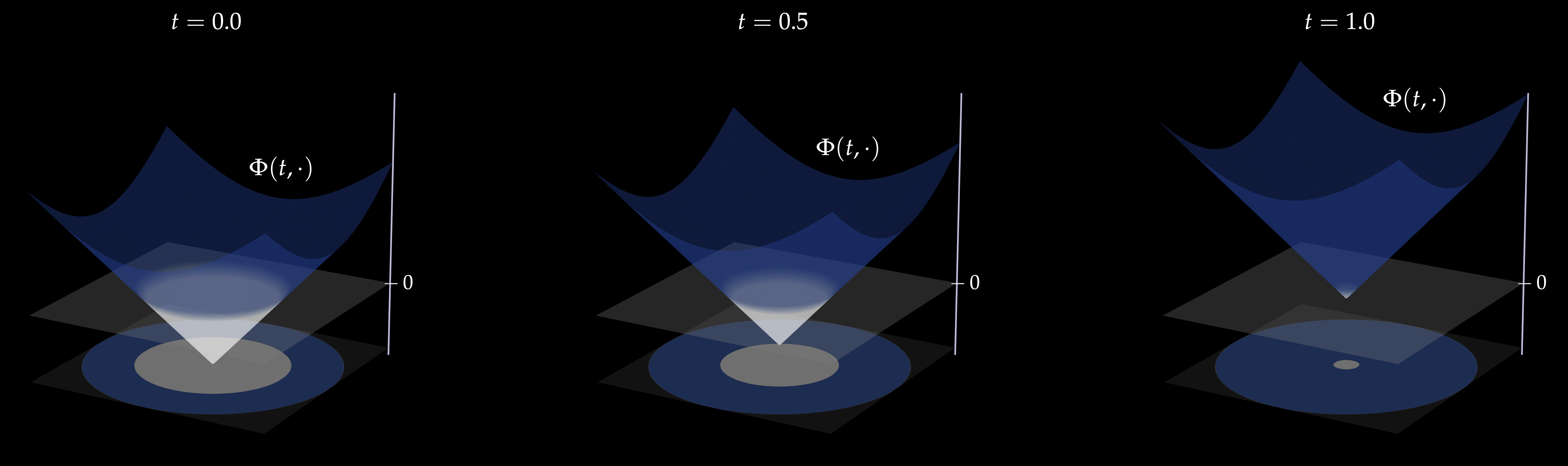
Figure 2: Time evolution of the level-set function in the radial case and projected solid region (bottom horizontal plane).

3.1 Loss Function and Training

Let us explain how the parameters in $\Gamma^{\theta}$ can be trained so as to find a probabilistic solution, which is equivalent to requiring the growth condition (4) to hold for every test function. This is similar to Leray type weak solutions of nonlinear partial differential equations that demand certain equations to be satisfied for a class of test functions, and our approach can possibly be applied to compute this type of solutions as well. We transform the growth condition into a loss function by forcing (4) to hold for a large but finite number of test functions. Specifically, letting $\Psi\subset\operatorname{\mathcal{C}}_{c}^{\infty}(\Omega)$ be a finite collection of test functions, we aim to

$$\text{minimize }\;\operatorname{\mathcal{L}}(\theta)=\sum_{\psi\in\Psi}\operatorname{\mathcal{L}}(\theta,\psi)\;\text{ over }\;\theta\in\Theta,\quad\text{where}$$ (12)

$$\operatorname{\mathcal{L}}(\theta,\psi)=\bigg{\lVert}\int_{\Gamma_{0-}}\psi-\int_{\Gamma^{\theta}_{\cdot}}\psi-\frac{1}{L}\big{(}\eta\ \mathbb{E}[\psi(X^{1}_{\tau^{1,\theta}})\,\mathds{1}_{\{\tau^{1,\theta}\ \leq\ \cdot\}}]-\mathbb{E}[\psi(X^{2}_{\tau^{2,\theta}})\,\mathds{1}_{\{\tau^{2,\theta}\ \leq\ \cdot\}}]\big{)}\bigg{\rVert}_{L^{2}([0,T])}^{2}.$$ (13)

We expect that $\Gamma^{\theta}$ induces a probabilistic solution if $\operatorname{\mathcal{L}}(\theta)=0$ and $\Psi$ grows to a dense subset of $\operatorname{\mathcal{C}}_{c}^{\infty}(\Omega)$. In order to compute the loss function in (12), we simulate reflected Brownian particles $X^{j}=(X_{t_{n}}^{j})_{t_{n}\in\Pi^{N}}$, $j=1,\ldots,J$, on a regular time grid $\Pi_{N}\mathrel{\mathop{\ordinarycolon}}=\{t_{n}=n\Delta t\!\mathrel{\mathop{\ordinarycolon}}n=0,\ldots,N\}$, $\Delta t=\frac{T}{N}$. This gives the empirical loss

$$\operatorname{\mathcal{L}}(\theta)=\sum_{\psi\in\Psi}\sum_{n=1}^{N}\ell_{n}(\theta,\psi)^{2},$$ (14)

$${\scriptsize\ell_{n}(\theta,\psi)}=\scriptsize\int_{\Gamma_{0-}}\psi-\int_{\Gamma^{\theta}_{t_{n}}}\psi-\ \frac{1}{JL}\sum_{j=1}^{J}\Big{(}\eta\ \psi(X^{1,j}_{\tau^{1,\theta,j}})\,\mathds{1}_{\{\tau^{1,\theta,j}\leq t_{n}\}}-\ \psi(X^{2,j}_{\tau^{2,\theta,j}})\,\mathds{1}_{\{\tau^{2,\theta,j}\leq t_{n}\}}\Big{)}.$$ (15)

We then train the deep level-set function by gradient descent. That is, the parameters are updated according to

$$\theta_{m+1}=\theta_{m}-\zeta_{m}\nabla_{\theta}\operatorname{\mathcal{L}}(\theta_{m}),\quad m=1,\ldots,M,$$ (16)

for some $M\in\operatorname{\mathbb{N}}$. However, the map $\theta\mapsto\tau^{\theta}$ is piecewise constant, where $\tau^{\theta}$ denotes a stopping time on the right-hand side of (15). For concreteness, let us suppose that $\tau^{\theta}$ is the exit time of a liquid particle from the liquid region. In terms of the parameterized level-set function, this reads

$$\tau^{\theta}=\inf\{t_{n},n\leq N\mathrel{\mathop{\ordinarycolon}}\,\Phi(t_{n},X_{t_{n}}^{1};\theta)<0\}.$$

Unless a trajectory $(X^{1}_{t_{n}}(\omega))_{n=0}^{N}$ is exactly on the solid-liquid interface at the stopping time $\tau^{\theta}(\omega)$, i.e., $\Phi(\tau^{\theta}(\omega),X_{\tau^{\theta}}^{1}(\omega);\theta)=0$, the value of $\tau^{\theta}(\omega)$ will remain the same after an infinitesimal change in the parameter vector $\theta$. Hence, the gradient descent would not converge due to the vanishing gradient $\nabla_{\theta}\tau^{\theta}$. To circumvent this issue, the stopping times are relaxed according to a procedure explained in the next section.

Regarding the test functions, we choose the Gaussian kernels

$$\Psi=\left\{\psi_{k}(x)=e^{-\beta_{k}|x-z_{k}|^{2}}\mathrel{\mathop{\ordinarycolon}}\,\beta_{k}>0,\ z_{k}\in\Omega,\ k=1,\ldots,K\right\},\quad K\in\operatorname{\mathbb{N}}.$$

The centers $z_{k}$ and widths $\beta_{k}$ are randomized in each training iteration to cover the whole domain and to capture a variety of scales.

3.2 Relaxed Stopping Times

We adapt the relaxation procedure of [34], proposed in the context of optimal stopping. In short, it consists of replacing the sharp boundary $\partial\Gamma_{t}$ by a mushy (or fuzzy) region where stopping may or may not take place. First, we transform the neural network $\Phi(t,\cdot\ ;\theta)$ to locally approximate the signed distance to the interface $\partial\Gamma_{t}$. This is achieved by normalization, namely by setting $\rho(t,\cdot\ ;\theta)=\frac{\Phi(t,\cdot\ ;\theta)}{|\nabla_{x}\Phi(t,\cdot\ ;\theta)|}$. We note that the spatial gradient of $\Phi(\cdot;\theta)$ can be exactly and effortlessly computed using automatic differentiation.

Next, the approximate signed distance is converted into a stopping probability. Without loss of generality, we describe the procedure for liquid particles which are stopped when entering the solid region. For solid particles, see Remark 3. Given $\varepsilon>0$, define the phase indicator variables

$$q^{\theta,\varepsilon}_{n}=(\chi^{\varepsilon}\circ\rho)(t_{n},X_{t_{n}}^{1};\theta),\quad n=0,\ldots,N,$$

with the relaxed phase function $\chi^{\varepsilon}(\rho)=\frac{(1-\rho/\varepsilon)^{+}}{2}\wedge 1$; see Fig. 3 for an illustration. The phase indicator variable is equal to $1$ in the “$\varepsilon-$interior” of the solid region (where $\rho(t,x;\theta)\leq-\varepsilon$) and is $0$ when $\rho(t,x;\theta)\geq\varepsilon$. Inside $\partial\Gamma_{t}^{\theta,\varepsilon}$, the phase indicator variable decreases linearly with the signed distance to the interface. The parameter $\varepsilon>0$ specifies the width of the mushy region

$$\partial\Gamma_{t}^{\theta,\varepsilon}=\{x\in\Omega\mathrel{\mathop{\ordinarycolon}}\,|\rho(t,x;\theta)|<\varepsilon\},$$

in which a liquid particle enters the solid region with probability $q^{\theta,\varepsilon}_{n}\in(0,1)$.

For Brownian particles, a natural choice for $\varepsilon$ is $\varepsilon=\sqrt{d\ \Delta t}$, this being the order of the typical Euclidean distance travelled by a $d$-dimensional standard Brownian motion over a time sub-interval $[t,t+\Delta t]$. For Brownian particles with diffusivity $\alpha>0$, we set instead $\varepsilon=\sqrt{\alpha d\Delta t}$. When the liquid and the solid particles have different diffusivities, we consider distinct mushy regions. Finally, the stopped values in (15) are replaced by

$$\psi(X_{\tau^{1,\theta}}^{1})\,\mathds{1}_{\{\tau^{1,\theta}\ \leq\ t_{n}\}}\approx\sum_{l=1}^{n}Q^{\theta,\varepsilon}_{l}\ \psi(X_{t_{l}}^{1}),$$

with the random stopping probabilities recursively given by

$$\quad Q_{n}^{\theta,\varepsilon}=q^{\theta,\varepsilon}_{n}\underbrace{\Big{(}1-\sum_{l<n}\ Q_{l}^{\theta,\varepsilon}\Big{)}}_{\text{same phase until $t_{n}$}},\quad n=0,\ldots,N.$$

Similarly, the integrals in (15) are computed as

$$\int_{\Gamma_{t_{n}}^{\theta}}\psi\ \approx\ \frac{|\Omega|}{J}\sum\limits_{j=1}^{J}q_{n,0,j}^{\theta,\varepsilon}\ \psi(U^{j}),\quad\ q_{n,0,j}^{\theta,\varepsilon}=(\chi^{\varepsilon}\circ\rho)(t_{n},U^{j};\theta),\quad U^{j}\overset{\text{i.i.d.}}{\sim}\ \text{Unif}(\Omega),$$ (17)

where Unif$(\Omega)$ is the uniform distribution on $\Omega$. Notice that the terms $\int_{\Gamma_{0-}}\psi_{k}$ do not depend on $\theta$ so they can be computed only once, e.g., in an offline phase. Because of the above relaxation, the gradient of $\operatorname{\mathcal{L}}(\theta)$ does not vanish anymore. We can therefore apply gradient descent to minimize the loss function, thus finding an approximation of the solid region $\Gamma$.

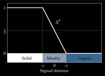
Figure 3: Illustration of the relaxed phase function $\chi^{\varepsilon}(\rho)=\frac{(1-\rho/\varepsilon)^{+}}{2}\wedge 1$.

Remark 3.

For solid particles, the phase indicator variables are defined analogously by

$$q^{\theta,\varepsilon}_{n}=1-(\chi^{\varepsilon}\circ\rho)(t_{n},X_{t_{n}}^{2};\theta).$$

We can thereafter follow the steps above to approximate the stopped values $\psi(X_{\tau^{2,\theta}}^{2})\,\mathds{1}_{\{\tau^{2,\theta}\ \leq\ t_{n}\}}$.

3.3 Jump penalty

So far, there is no control on the change in volume of the solid region. Although jumps can be observed [12], we may find a solution which satisfies the growth condition but exhibits non-physical jumps, i.e., jumps of non-physically large size. To deal with this issue, we consider the more general loss function $\underline{\operatorname{\mathcal{L}}}(\theta)=\operatorname{\mathcal{L}}(\theta)+\lambda\operatorname{\mathcal{P}}(\theta)$, with the penalty term

$$\operatorname{\mathcal{P}}(\theta)=\operatorname{\mathcal{R}}\Big{(}\max\limits_{n=1,\ldots,N}|\Gamma^{\theta}_{t_{n}}\triangle\Gamma^{\theta}_{t_{n-1}}|-C\Big{)},\quad C>0,\quad\operatorname{\mathcal{R}}(\Delta)=\Delta^{+}-0.01\Delta^{-},$$ (18)

where $\triangle$ is the symmetric difference operation, and $C>0$ is a constant describing the “allowed” volume increment between time steps. We note that $\operatorname{\mathcal{R}}$ is the so-called Leaky ReLU activation function, whose choice is justified as follows. If the maximum change in volume exceeds the threshold $C$, the deep level-set function is severely penalized by the “ReLU” part of $\operatorname{\mathcal{R}}$ (namely, $\Delta^{+}$). On the other hand, the “leaky” part of $\operatorname{\mathcal{R}}$, i.e., $0.01\Delta^{-}$, is introduced to slightly incentivize the solid to shrink/grow smoothly over time.

The Lagrange multiplier $\lambda$ is decomposed into the product of a fixed ratio $\lambda_{0}>0$ (typically less than one) and a dynamically updated factor $\lambda^{\text{\tiny scale}}$ such that $\lambda^{\text{\tiny scale}}\ \nabla_{\theta}\operatorname{\mathcal{P}}(\theta)$ matches the scale of the gradient $\nabla_{\theta}\operatorname{\mathcal{L}}(\theta)$. For this task, we employ the “learning rate annealing algorithm” outlined in Wang et al. [46]. It is a popular normalization technique for physics-informed neural networks when the loss function comprises heterogeneous components. Finally, the volume of $\Gamma^{\theta}_{t_{n}}\triangle\ \Gamma^{\theta}_{t_{n-1}}$ is estimated using a Monte Carlo simulation as in (17).

Throughout the numerical experiments, we set the jump threshold to $C=\frac{|\Omega|}{2}$. In other words, the solid region is told to grow/shrink by at most half the size of the domain per time step. This is a loose constraint, which nevertheless rules out undesirable time discontinuities as we shall see in the numerical experiments. At the same time, we shall see in Section 4.1.4 that the regularized algorithm is still capable of producing physical jumps, whose definition is now recalled. We also refer the interested reader to [25]. Let us focus on the radial case and consider for $r\geq 0$, $\Delta\in\operatorname{\mathbb{R}}$, the annulus

$$A_{r,\Delta}\mathrel{\mathop{\ordinarycolon}}=\begin{cases}B_{r+\Delta}\setminus B_{r},&\Delta\geq 0,\\ B_{r}\setminus B_{r+\Delta},&-r\leq\Delta<0,\\ B_{r},&\Delta<-r.\end{cases}$$ (19)

A radial solution $(\Gamma_{t})_{t\in[0,T]}=(B_{r(t)})_{t\in[0,T]}$ to the Stefan problem is physical if for all $t\in[0,T]$, the jump $\Delta r(t)=r(t)-r(t-)$, if positive, satisfies

$$\Delta r(t)=\inf\bigg{\{}\Delta>0\ \mathrel{\mathop{\ordinarycolon}}\ |A_{r(t-),\Delta}|>-\frac{1}{L}\int_{A_{r(t-),\Delta}}u^{1}(t-,x)\bigg{\}}.$$ (20)

If $\Delta r(t)=r(t)-r(t-)>0$, we gather that for physical solutions, $\Delta r(t)$ is the smallest solution of

$$|A_{r(t-),\Delta}| =-\frac{1}{L}\int_{A_{r(t-),\Delta}}u^{1}(t-,x).$$ (21)

The left-hand side in (21) is the volume absorbed by the solid region $\Gamma$ at time $t$. The right-hand side in (21) is the aggregate change in temperature upon freezing of $A_{r(t-),\Delta}$.

Remark 4.

In the non-radial case, it is not sufficient to consider the volume increments only. The formulation of an appropriate physicality condition is in fact subject of ongoing research.

3.4 Algorithm

The deep level-set method is summarized in Algorithm 1. The learning rate process $(\zeta_{m})_{m=1}^{M}$ is computed using the Adam optimizer [20]. For the Monte Carlo simulation of particles, we use antithetic sampling to explore the domain in a symmetric fashion and to speed up computation. More specifically, we simulate two antithetic particles for each generated initial point $x_{0}^{i}$, namely

$$X^{i}_{\cdot} =x_{0}^{i}+\sqrt{\alpha_{i}}\ W_{\cdot\wedge\tau^{i}}^{i}+l_{\cdot\wedge\tau^{i}}^{i},\quad\tau^{i}=\inf\{t\in[0,T]\mathrel{\mathop{\ordinarycolon}}\,x_{0}^{i}+\sqrt{\alpha_{i}}\ W_{t}^{i}+l^{i}_{t}\notin\Gamma_{t}^{i}\},$$

$$\widetilde{X}^{i}_{\cdot} =x_{0}^{i}-\sqrt{\alpha_{i}}\ W_{\cdot\wedge\widetilde{\tau}^{i}}^{i}+\widetilde{l}_{\cdot\wedge\widetilde{\tau}^{i}}^{i},\quad\widetilde{\tau}^{i}=\inf\{t\in[0,T]\mathrel{\mathop{\ordinarycolon}}\,x_{0}^{i}-\sqrt{\alpha_{i}}\ W_{t}^{i}+\widetilde{l}_{t}^{i}\notin\Gamma_{t}^{i}\}.$$

Algorithm 1 (Deep level-set method)

Given: $\Phi_{0}=$ initial level-set function, $J=$ batch size, $M=$ # training iterations, $\Psi=$ set of test functions, $C=$ jump constant, $\varepsilon=$ mushy region width
 

• Initialize $\theta_{0}\in\Theta$

• For $m=0,\ldots,M-1$:

  1. Simulate $X^{i,j}=(X_{t_{n}}^{i,j})_{n=0}^{N}$ ($i=1$: liquid, $i=2$: solid), $\ U^{j}\ \overset{\text{i.i.d.}}{\sim}\ \text{Unif}(\Omega)$, $j=1,\ldots,J$

  2. Approximate the signed distance function of $\partial\Gamma$ as $\rho(\cdot;\theta_{m})=\frac{\Phi(\cdot;\ \theta_{m})}{|\nabla_{x}\Phi(\cdot;\ \theta_{m})|}$

  3. For $n=0,\ldots,N$, $\psi\in\Psi$, compute:

     • Phase indicator variables: $q_{n,i,j}^{\theta_{m},\varepsilon}=\begin{cases}(\chi^{\varepsilon}\circ\rho)(t_{n},U^{j};\theta_{m}),&i=0,\\[1.99997pt] (\chi^{\varepsilon}\circ\rho)(t_{n},X_{t_{n}}^{1,j};\theta_{m}),&i=1,\\[1.99997pt] 1-(\chi^{\varepsilon}\circ\rho)(t_{n},X_{t_{n}}^{2,j};\theta_{m}),&i=2\\ \end{cases}$

     • Symmetric Differences: $|\Gamma^{\theta_{m}}_{t_{n}}\triangle\Gamma^{\theta_{m}}_{t_{n-1}}|\approx\frac{|\Omega|}{J}\sum\limits_{j=1}^{J}|q_{n,0,j}^{\theta_{m},\varepsilon}-q_{n-1,0,j}^{\theta_{m},\varepsilon}|$
       

     • Integrals: $\int_{\Gamma^{\theta_{m}}_{t_{n}}}\psi\ \approx\ \frac{|\Omega|}{J}\sum\limits_{j=1}^{J}q_{n,0,j}^{\theta_{m},\varepsilon}\ \psi(U^{j})$
       

     • Stopping probabilities: $Q_{n,i,j}^{\theta_{m},\varepsilon}=q_{n,i,j}^{\theta_{m},\varepsilon}(1-\sum\limits_{l<n}Q_{l,i,j}^{\theta_{m},\varepsilon}),\;i=1,2$
       

     • Stopped values: $\psi(X^{i,j}_{\tau^{\theta_{m}}})\,\mathds{1}_{\{\tau^{\theta_{m}}\leq t_{n}\}}\approx\sum\limits_{l=1}^{n}Q_{l,i,j}^{\theta_{m},\varepsilon}\psi(X_{t_{l}}^{i,j})$
       

  4. Loss: $\operatorname{\mathcal{L}}(\theta_{m})=\sum\limits_{\psi\in\Psi}\sum\limits_{n=1}^{N}\ell_{n}(\theta_{m},\psi)^{2}$, with

     $${\scriptsize\ell_{n}(\theta_{m},\psi)} ={\scriptsize\int_{\Gamma_{0-}}\!\psi-\int_{\Gamma^{\theta_{m}}_{t_{n}}}\!\psi}$$

     $$-{\scriptsize\ \frac{1}{JL}\sum_{j=1}^{J}\Big{(}\eta\ \psi(X^{1,j}_{\tau^{1,\theta_{m},j}})\,\mathds{1}_{\{\tau^{1,\theta_{m},j}\leq t_{n}\}}-\ \psi(X^{2,j}_{\tau^{2,\theta_{m},j}})\,\mathds{1}_{\{\tau^{2,\theta_{m},j}\leq t_{n}\}}\Big{)}}$$

  5. Jump penalty: $\ \operatorname{\mathcal{P}}(\theta_{m})=\operatorname{\mathcal{R}}\Big{(}\max\limits_{n=1,\ldots,N}|\Gamma^{\theta_{m}}_{t_{n}}\triangle\Gamma^{\theta_{m}}_{t_{n-1}}|-C\Big{)}$
     

  6. Gradient step: $\theta_{m+1}=\theta_{m}-\zeta_{m}\nabla_{\theta}\underline{\operatorname{\mathcal{L}}}(\theta_{m})$, $\;\underline{\operatorname{\mathcal{L}}}(\theta_{m})=\operatorname{\mathcal{L}}(\theta_{m})+\lambda_{0}\ \lambda_{m}^{\text{\tiny scale}}\operatorname{\mathcal{P}}(\theta_{m})$

• Return $\Gamma^{\theta_{M}}=\{\Phi(\cdot\ ;\theta_{M})\leq 0\}$
  

3.5 Adding surface tension

3.5.1 Growth Condition Revisited

The numerical verification of the growth condition given in Definition 2 is not straightforward because of the additional term $\operatorname{\mathcal{K}}_{t}$. It turns out that an alternative formulation, which we now outline, greatly simplifies the implementation. In what follows, we assume that $d\geq 2$. For $\delta>0$, define the one-sided mushy regions,

$$\partial\Gamma_{t}^{\delta,i}=\{x\in\Gamma_{t}^{i}\mathrel{\mathop{\ordinarycolon}}\,dist(x,\partial\Gamma_{t})\leq\delta\},\quad i=1,2.$$

Let $(T_{l}^{\delta,i})_{l\geq 1}$ be the arrival times of a time-space Poisson point process with intensity

$$\lambda^{i}(t,y)=\frac{\gamma}{\delta}|\kappa_{\partial\Gamma_{t}}(\widehat{y})|^{2-d}\frac{\mathds{1}_{\partial\Gamma_{t}^{\delta,i}}(y)}{|\partial\Gamma_{t}^{\delta,i}|},\quad\widehat{y}=\text{proj}_{\partial\Gamma_{t}}(y),\quad d\geq 2,$$ (22)

where $\text{proj}_{\partial\Gamma_{t}}(y)$ is the projection of $y$ onto $\partial\Gamma_{t}$, i.e., the point on $\partial\Gamma_{t}$ closest to $y$. For each $l\geq 1$ and $i=1,2$, we simulate a Brownian particle $Y^{l,i}=(Y^{l,i}_{s})_{s\in[T_{l}^{\delta,i},T]}$ where, according to (22), the initial position of $Y^{l,i}$ is uniformly distributed in $\partial\Gamma_{T^{\delta,i}_{l}}^{\delta,i}$ if $d=2$ and inversely proportional to the absolute mean curvature of $\partial\Gamma_{T^{\delta,i}_{l}}$ otherwise. We also define the exit times $\tau_{l}^{\delta,i}=\inf\{s\geq T^{\delta,i}_{l}\!\mathrel{\mathop{\ordinarycolon}}Y^{l,i}_{s}\notin\Gamma_{s}^{i}\}$.

In the three-dimensional, radially symmetric case (namely $\Gamma_{t}=B_{r(t)}\subseteq\operatorname{\mathbb{R}}^{3}$), the Poisson intensities simply read

$${\lambda^{i}(t,\cdot)=\frac{\gamma}{\delta}}r(t)\frac{\mathds{1}_{A_{r(t),\Delta_{i}}}}{|A_{r(t),\Delta_{i}}|},\quad\Delta_{i}=(-1)^{i+1}\delta,$$ (23)

with the annuli $A_{r,\Delta}$ defined in (19). We therefore gather that the expected number of simulated particles is directly proportional to the radius of the solid region.

Proposition 3.

Assume that $\alpha_{1}=\alpha_{2}$ and consider a classical solution of the radially symmetric Stefan problem with surface tension. Moreover, let $N_{t}^{\delta,i}\mathrel{\mathop{\ordinarycolon}}=\sum_{l=1}^{\infty}\mathds{1}_{\{T^{\delta,i}_{l}\leq t\}}$ be the counting process associated with $(T^{\delta,i}_{l})$, $i=1,2$. Then for all $\psi\in\mathcal{C}_{c}^{\infty}(\Omega)$,

$$\int_{\Gamma_{0-}}\psi-\int_{\Gamma_{t}}\psi=\frac{1}{L}\Big{(}\eta\operatorname{\mathbb{E}}^{\mu^{1}}[\psi(X_{\tau^{1}}^{1})\,\mathds{1}_{\{\tau^{1}\leq t\}}]-\operatorname{\mathbb{E}}^{\mu^{2}}[\psi(X_{\tau^{2}}^{2})\,\mathds{1}_{\{\tau^{2}\leq t\}}]+\operatorname{\mathcal{K}}_{t}\Big{)},$$ (24)

$$\operatorname{\mathcal{K}}_{t}=-\operatorname{\mathcal{K}}_{t}^{1}-\operatorname{\mathcal{K}}_{t}^{2},$$ (25)

$$\operatorname{\mathcal{K}}_{t}^{i}=\lim_{\delta\downarrow 0}\ \operatorname{\mathbb{E}}\Bigg{[}\sum_{l=1}^{N_{t}^{\delta,i}}\Big{(}\psi(Y_{\tau_{l}^{\delta,i}}^{l,i})\,\mathds{1}_{\{\tau^{\delta,i}_{l}\leq t\}}\ {-\ \psi(Y_{T^{\delta,i}_{l}}^{l,i})}\Big{)}\Bigg{]}.$$ (26)

Proof.

See Section A.3. ∎

Remark 5.

When the diffusivities of the solid and the liquid phase are different ($\alpha_{1}\neq\alpha_{2}$), the right-hand side of the growth condition (24) contains an additional term, namely

$$\widetilde{\operatorname{\mathcal{K}}}_{t}=-\gamma\frac{\alpha_{2}-\alpha_{1}}{2}\int_{0}^{t}\int_{\partial\Gamma_{s}}\kappa_{\partial\Gamma_{s}}\ \partial_{\nu}\psi.$$

Recalling that $u^{1}=u^{2}=-\gamma\kappa_{\partial\Gamma_{s}}$, the above term can be approximated via

$$\widetilde{\operatorname{\mathcal{K}}}_{t}\approx\frac{\alpha_{2}}{2\delta}\int_{0}^{t}\int_{\partial\Gamma_{s}^{\delta,2}}u^{2}\ \partial_{\nu}\psi-\frac{\alpha_{1}}{2\delta}\int_{0}^{t}\int_{\partial\Gamma_{s}^{\delta,1}}u^{1}\ \partial_{\nu}\psi.$$

The integrals $\int_{\partial\Gamma_{s}^{\delta,i}}u^{i}\ \partial_{\nu}\psi$, in turn, can be computed using the stochastic representation of $u^{i}$ given in (41), below. Note that $\partial_{\nu}\psi$ is easy to compute since the outward normal $\nu$ is available from the deep level-set function.

Remark 6.

It is conjectured that the representation (26) of the curvature terms holds beyond the radial case. The only difference is that the effect of boundary particles is reversed in concave sections of the boundary. Specifically, we expect that, in general,

$$\operatorname{\mathcal{K}}_{t}^{i}=\lim_{\delta\downarrow 0}\ \operatorname{\mathbb{E}}\Bigg{[}\sum_{l=1}^{N_{t}^{\delta,i}}\text{sign}\big{(}\kappa_{\partial\Gamma_{\!T_{l}^{\delta,i}}}(\widehat{Y_{T^{\delta,i}_{l}}^{l,i}})\big{)}\big{(}\psi(Y_{\tau_{l}^{\delta,i}}^{l,i})\,\mathds{1}_{\{\tau_{l}^{\delta,i}\leq t\}}\ -\ \psi(Y_{T^{\delta,i}_{l}}^{l,i})\big{)}\Bigg{]}.$$ (27)

We show how to approximate $\operatorname{\mathcal{K}}_{t}^{i}$ of (27). First, the mushy regions can be expressed in terms of the level-set function as follows:

$$\partial\Gamma_{t}^{\delta,1}\approx\left\{x\in\Omega\mathrel{\mathop{\ordinarycolon}}\,\frac{\Phi(t,x)}{|\nabla_{x}\Phi(t,x)|}\in(0,\delta]\right\},\quad\partial\Gamma_{t}^{\delta,2}\approx\left\{x\in\Omega\mathrel{\mathop{\ordinarycolon}}\,\frac{\Phi(t,x)}{|\nabla_{x}\Phi(t,x)|}\in[-\delta,0]\right\}.$$

Without loss of generality, we focus on the term $\operatorname{\mathcal{K}}_{t}^{1}$ and drop the superscripts ¹ throughout. Using the time discretization $\{t_{n}=n\Delta t\!\mathrel{\mathop{\ordinarycolon}}n=0,\ldots,N\}$, $\Delta t=\frac{T}{N}$, $N\in\operatorname{\mathbb{N}}$, we obtain for $\delta>0$ sufficiently small that

$$\operatorname{\mathcal{K}}_{t_{n}}\approx\ \sum_{m=0}^{n-1}\operatorname{\mathbb{E}}\Bigg{[}\sum_{l=N^{\delta}_{t_{m}}{+1}}^{N^{\delta}_{t_{m+1}}}\operatorname{\mathbb{E}}\Big{[}\text{sign}\big{(}\kappa_{\partial\Gamma_{\!t_{m}}}(\widehat{Y_{t_{m}}^{l}})\big{)}\big{(}\psi(Y_{\tau_{l}^{\delta}}^{l})\,\mathds{1}_{\{\tau_{l}^{\delta}\leq t_{n}\}}-\psi(Y_{t_{m}}^{l})\big{)}\ \Big{|}\ T^{\delta}_{l}=t_{m}\Big{]}\Bigg{]}.$$

Writing $\operatorname{\mathbb{E}}_{t_{m},y}[\cdot]=\operatorname{\mathbb{E}}[\ \cdot\ |\ T^{\delta}_{l}=t_{m},\ Y^{l}_{t_{m}}=y]$ and recalling the Poisson intensity in (22) we find that

$$\,\operatorname{\mathcal{K}}_{t_{n}}\approx\ \sum_{m=0}^{n-1}\frac{\gamma\Delta t}{\delta\ |\partial\Gamma_{t_{m}}^{\delta}|}\int_{\partial\Gamma_{t_{m}}^{\delta}}|\kappa_{\partial\Gamma_{t_{m}}}(\widehat{y})|^{2-d}\operatorname{\mathbb{E}}_{t_{m},y}\big{[}\text{sign}\big{(}\kappa_{\partial\Gamma_{\!t_{m}}}(\widehat{y})\big{)}\big{(}\psi(Y_{\tau^{\delta}})\,\mathds{1}_{\{\tau^{\delta}\leq t_{n}\}}-\psi(y)\big{)}\big{]}\,\mathrm{d}y$$

$$=\ \frac{\gamma\Delta t}{\delta}\sum_{m=0}^{n-1}\operatorname{\mathbb{E}}\Big{[}\ \text{sign}\big{(}\kappa_{\partial\Gamma_{t_{m}}}(\widehat{Y_{t_{m}}})\big{)}\big{|}\kappa_{\partial\Gamma_{t_{m}}}(\widehat{Y_{t_{m}}})\big{|}^{2-d}\operatorname{\mathbb{E}}\big{[}\psi(Y_{\tau^{\delta}})\,\mathds{1}_{\{\tau^{\delta}\leq t_{n}\}}{-\psi(Y_{t_{m}})}\ \big{|}\ T^{\delta}=t_{m},\ Y_{t_{m}}\big{]}\Big{]}.$$ (28)

The latter is estimated through Monte Carlo simulation where, for simplicity, the curvature is evaluated at $Y_{t_{m}}$ instead of its projection $\widehat{Y_{t_{m}}}$ onto $\partial\Gamma_{t_{m}}$. This is an accurate approximation of the “true” curvature when the width $\delta$ of the mushy region is small. What remains is to approximate the mean curvature, which we address in the next section.

3.5.2 Mean Curvature Approximation

In this section, we present simple algorithms to locally approximate the mean curvature of a manifold $\Sigma\subset\operatorname{\mathbb{R}}^{d}$, $d=2,3$, of codimension $1$. Other techniques, e.g., using finite differences, are discussed in [31]. If $\Sigma=\{\phi=0\}$ for some level-set function $\phi\in\operatorname{\mathcal{C}}^{2}(\operatorname{\mathbb{R}}^{d})$, the mean curvature can be expressed as

$$\kappa_{\Sigma}(y)=\frac{\text{div}\left(\nu(y)\right)}{d-1},\quad y\in\Sigma,$$ (29)

with the outward normal vector field $\nu=\frac{\nabla\phi}{|\nabla\phi|}$. If $\phi$ is parameterized by a neural network, one could apply automatic differentiation to compute $\kappa_{\Sigma}$. But computing second order derivatives through automatic differentiation is costly since it entails nested gradient tapes. Indeed, the machine would need to keep track of the first order derivatives as well. Alternative approaches have been proposed to speed up computation, e.g., using Monte Carlo techniques [36]. Here, we propose a dilation approach echoing the geometric nature of curvature and solely exploiting the gradient of $\phi$.

Figure 4: Dilation technique to capture the mean curvature of codimension $1$ interfaces in $\operatorname{\mathbb{R}}^{d}$, $d=2,3$.

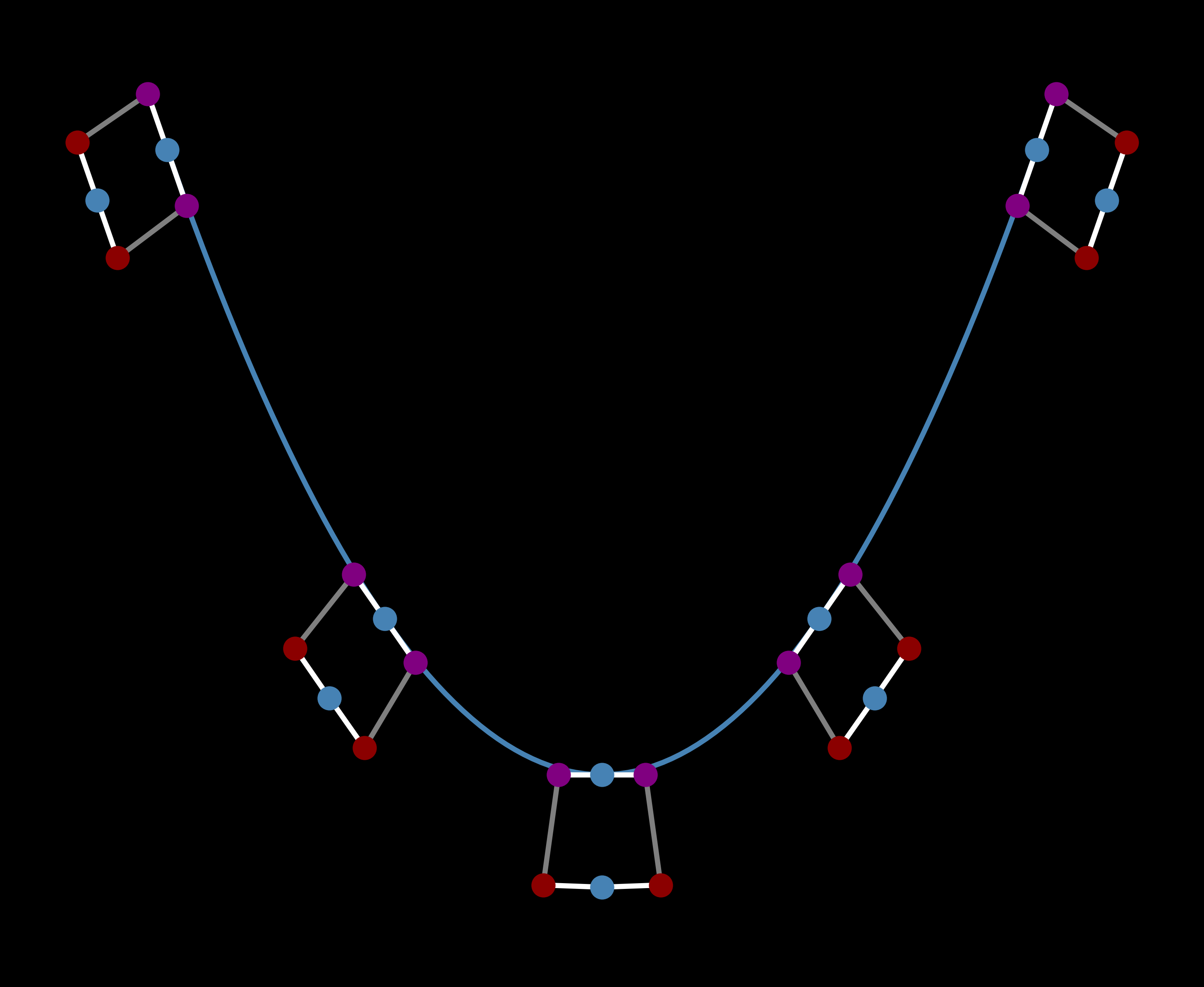
(a) $d=2$

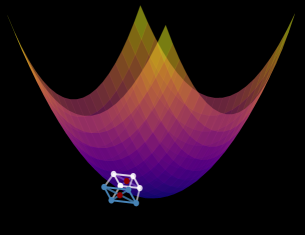
(b) $d=3$

As a motivation, consider a circle $\Sigma_{r}=\partial B_{r}\subseteq\operatorname{\mathbb{R}}^{2}$ of radius $r$ whose curvature is $\kappa_{\Sigma_{r}}=\frac{1}{r}$. One way to approximate the curvature is to look at the ratio between arc lengths of $\Sigma_{r}$ and the dilated circle $\Sigma_{r+\epsilon}$ for small $\epsilon>0$. Indeed, writing $\Sigma_{r}\supset\operatorname{\mathcal{A}}_{r,\epsilon_{0}}=\{(r\cos(t\epsilon_{0}),r\sin(t\epsilon_{0}))\!\mathrel{\mathop{\ordinarycolon}}t\in[0,1]\}$ for an arc with radius $r$ and angle $\epsilon_{0}\in[0,2\pi)$ we see that

$$\frac{\operatorname{\mathcal{H}}^{1}(\operatorname{\mathcal{A}}_{r+\epsilon,\epsilon_{0}})}{\operatorname{\mathcal{H}}^{1}(\operatorname{\mathcal{A}}_{r,\epsilon_{0}})}=\frac{\epsilon_{0}(r+\epsilon)}{\epsilon_{0}r}=1+\epsilon\ \kappa_{\Sigma_{r}}\;\Longrightarrow\;\kappa_{\Sigma_{r}}=\frac{1}{\epsilon}\bigg{(}\frac{\operatorname{\mathcal{H}}^{1}(\operatorname{\mathcal{A}}_{r+\epsilon,\epsilon_{0}})}{\operatorname{\mathcal{H}}^{1}(\operatorname{\mathcal{A}}_{r,\epsilon_{0}})}-1\bigg{)}.$$ (30)

We can mimic this procedure for general subsets $\Sigma\subset\operatorname{\mathbb{R}}^{2}$, $\text{dim}_{\operatorname{\mathcal{H}}}(\Sigma)=1$, by approximating $\Sigma$ locally by a circle. The procedure is summarized in Algorithm 2 where $\Sigma$ is the zero level set of some function $\phi\in\operatorname{\mathcal{C}}^{1}(\operatorname{\mathbb{R}}^{2})$. An illustration is also given in Fig. 4(a). When $\epsilon_{0}>0$ is small, the arc of length $\epsilon_{0}$ in (30) is accurately replaced by a segment tangent to $\Sigma$. We recall that the outward normal vector field of $\Sigma$ is readily available from the level-set function. The tangent vector field is therefore available as well.

Algorithm 2 (Local approximation of curvature, $d=2$)

Given: $\phi\in\operatorname{\mathcal{C}}^{1}(\Omega)$ $(\nabla\phi\neq 0)$, $\ \Sigma=\{\phi=0\}$, $\ y\in\Sigma$, $\ \epsilon_{0}>0,\ \epsilon>0$
 

• Pick a direction $\mu$ of the tangent line at $y$, i.e., perpendicular to $\nu(y)=\frac{\nabla\phi(y)}{|\nabla\phi(y)|}$

• Consider
  

  1. the segment $S_{y}\subseteq\operatorname{\mathbb{R}}^{2}$ with endpoints $y^{\pm}=y\pm\epsilon_{0}\mu$

  2. the dilated segment $S^{\epsilon}_{y}\subseteq\operatorname{\mathbb{R}}^{2}$ with endpoints $y^{\pm}+\epsilon\ \nu(y^{\pm})$

• Compute the ratio $\frac{\mathcal{H}^{1}(S^{\epsilon}_{y})}{\mathcal{H}^{1}(S_{y})}\approx 1+\epsilon\ \kappa_{\Sigma}(y)$

• Return the curvature $\kappa_{\Sigma}(y)\approx\frac{1}{\epsilon}\Big{(}\frac{\mathcal{H}^{1}(S^{\epsilon}_{y})}{\mathcal{H}^{1}(S_{y})}-1\Big{)}$
  

A similar procedure can be used in the three-dimensional case, as explained in Algorithm 3 and displayed in Fig. 4(b). In short, the segments in Algorithm 2 become quadrangles and lengths are replaced by areas. In Step III of Algorithm 3, note that the mean curvature appears naturally from the cross products in $(1+\epsilon\kappa_{\Sigma,1})(1+\epsilon\kappa_{\Sigma,2})$, where $(\kappa_{\Sigma,i})_{i=1}^{2}$ are the principal curvatures of $\Sigma$. As the principal directions are unknown in general, the algorithm picks randomly two orthogonal vectors in the plane tangent to $\Sigma$ at some point $y\in\Sigma$. This randomization has little impact on the accuracy of the obtained, as can be seen in Fig. 5(b) and Fig. 6(d).

Algorithm 3 (Local approximation of mean curvature, $d=3$)

Given: $\phi\in\operatorname{\mathcal{C}}^{1}(\Omega)$ $(\nabla\phi\neq 0)$, $\ \Sigma=\{\phi=0\}$, $\ y\in\Sigma$, $\ \epsilon_{0}>0,\ \epsilon>0$
 

• Pick two directions $\mu_{1}\perp\mu_{2}$ in the tangent plane at $y$, i.e., perpendicular to $\nu(y)=\frac{\nabla\phi(y)}{|\nabla\phi(y)|}$

• Consider
  

  1. the quadrangle $Q_{y}$ with vertices $y_{i}^{\pm}=y\pm\epsilon_{0}\mu_{i},\ i=1,2$

  2. the quadrangle $Q^{\epsilon}_{y}$ with vertices $y_{i}^{\pm}+\epsilon\ \nu(y_{i}^{\pm}),\ i=1,2$

• Compute the ratio $\frac{\mathcal{H}^{2}(Q^{\epsilon}_{y})}{\mathcal{H}^{2}(Q_{y})}\approx(1+\epsilon\ \kappa_{\Sigma,1}(y))(1+\epsilon\ \kappa_{\Sigma,2}(y))\approx 1+2\epsilon\ \kappa_{\Sigma}(y)$

• Return the mean curvature $\kappa_{\Sigma}(y)\approx\frac{1}{2\epsilon}\Big{(}\frac{\mathcal{H}^{2}(Q^{\epsilon}_{y})}{\mathcal{H}^{2}(Q_{y})}-1\Big{)}$
  

Back to the Stefan problem, we naturally choose $\Sigma=\partial\Gamma_{t}$, $t\in[0,T]$, and $\epsilon\ll\epsilon_{0}\ll\delta$, where $\delta$ is the width of the fuzzy regions $\partial\Gamma_{t}^{\delta,1}$, $\partial\Gamma_{t}^{\delta,2}$. Indeed, $\epsilon\ll\epsilon_{0}$ is imposed to gain accuracy while $\epsilon_{0}\ll\delta$ ensures that the points $y^{\pm}$ in Algorithm 2 ($y_{i}^{\pm}$ in Algorithm 3) belong to the fuzzy region for all $y\in\partial\Gamma_{t}$.

Let us verify Algorithms 2 and 3, respectively, for parabolas $\Sigma_{a}\mathrel{\mathop{\ordinarycolon}}=\{y\in\operatorname{\mathbb{R}}^{2}\!\mathrel{\mathop{\ordinarycolon}}y_{2}=\frac{y_{1}^{2}}{a}\}$ and paraboloids $\Sigma_{a,b}\mathrel{\mathop{\ordinarycolon}}=\{y\in\operatorname{\mathbb{R}}^{3}\!\mathrel{\mathop{\ordinarycolon}}y_{3}=\frac{y_{1}^{2}}{a}+\frac{y_{2}^{2}}{b}\}$ with parameters $a,b\in\operatorname{\mathbb{R}}\setminus\{0\}$. The mean curvature functions are given, respectively, by

$$\kappa_{\Sigma_{a}}(y)=\frac{2}{a\left(1+\frac{4y_{1}^{2}}{a^{2}}\right)^{3/2}}\quad(d=2),\qquad\kappa_{\Sigma_{a,b}}(y)=\frac{\frac{4y_{1}^{2}}{a}+\frac{4y_{2}^{2}}{b}+a+b}{ab\left(1+\frac{4y_{1}^{2}}{a^{2}}+\frac{4y_{2}^{2}}{b^{2}}\right)^{3/2}}\quad(d=3).$$ (31)

Fig. 5(b) shows the approximated curvature and the error relative to (31) for a parabola $(d=2)$ with parameter $a=2$. In Fig. 6(d), we repeat the exercise for a paraboloid with parameters $(a,b)=(1,2)$ (top panels) and a hyperbolic paraboloid with $(a,b)=(-1,2)$ (bottom panels). As expected, we note that the error for the hyperbolic paraboloid in Fig. 6(d) is only sizeable along the points with zero mean curvature.

Figure 5: Estimated curvature (left panel) and relative error (right panel) for a parabola $(d=2)$ with parameter $a=2$.

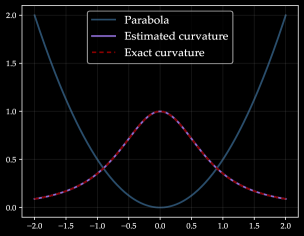
(a) Curvature

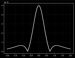
(b) Relative error

Figure 6: Estimated mean curvature (left panels) and relative error (right panels) for a paraboloid $(d=3)$ with parameters $(a,b)=(1,2)$ (top panels) and $(a,b)=(-1,2)$ (bottom panels).

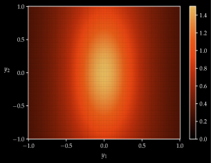
(a) Mean Curvature, $(a,b)=(1,2)$

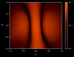
(b) Relative error, $(a,b)=(1,2)$

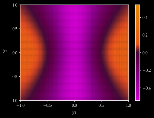
(c) Mean Curvature, $(a,b)=(-1,2)$

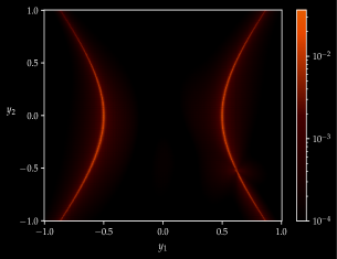
(d) Relative error, $(a,b)=(-1,2)$

4 Numerical Results

Table 1 and Table 2 report the default training and problem parameters, respectively, across the examples. The value of $M$ in Table 1 ($3000$) indicates the maximum number of iterations if the loss function has not stabilized yet. For the algorithm with surface tension, we set $M=1000$ as each training iteration is more costly. Note that the Lagrange multiplier in front of the penalty function is less than one to give more importance to the loss term than the penalty. The deep-level set function in (11) consists of a feedforward neural network with input $(t,x)$ of size $\bar{d}=d+1$ and two hidden layers with $20+\bar{d}\$ hidden nodes. The code is implemented in Python 3.9 using Tensorflow 2.7 and run on CPU ($10$ cores) on a 2021 Macbook pro with 64GB unified memory and Apple M1 Max chip.

Table 1: Default Training Parameters ($d=$ number of space dimensions)

Parameter	Definition	Value
$J$	Batch size	$2^{7+d}$
$M$	Number of training iterations	$3000$
$K$	Number of test functions $(|\Psi|)$	$100d$
$N$	Number of time steps	$100$
$\varepsilon_{i}$	Mushy region width of phase $i\in\{1,2\}$	$\sqrt{\alpha_{i}d\frac{T}{N}}$
$\lambda_{0}$	Lagrange multiplier	$0.1$

Table 2: Default problem parameters

Parameter	Definition	Value
$T$	Time horizon	$1$
$R$	Radius of spherical domain $\Omega$	$1$
$\alpha_{1}$	Diffusivity of liquid particles	$0.5$
$\alpha_{2}$	Diffusivity of solid particles	$0.5$
$\gamma$	Surface tension coefficient	$0$

4.1 Radial Case

We first discuss examples where the solid is radially symmetric. For concreteness, we regard the solid as an ice ball surrounded by (liquid) water.

4.1.1 One-phase, Melting Regime $(d=2)$

Consider the one-phase Stefan problem without surface tension as in Example 1. Given $\Gamma_{0-}=B_{1/2}\subset B_{1}=\Omega$, and assuming the initial temperature $u_{0}^{1}$ to be radially symmetric, the solid (ice) remains radial as well, i.e., $\Gamma_{t}=B_{r(t)}$ for some càdlàg function $r\!\mathrel{\mathop{\ordinarycolon}}[0,T]\to[0,R]$. We also set $\eta=1$, and $L=1/4$. The temperature in the liquid (water) is initially constant, namely $u^{1}_{0}\equiv\frac{1}{|B_{R}\setminus B_{r_{0}}|}$.

Fig. 8 compares the behavior of $r(t)$ as $t$ approaches the melting time with the theoretical asymptotic rate given by Hadzic and Raphael [16], namely

$$r(t)\ \sim\ \sqrt{\tau_{\varnothing}-t}\,e^{-\sqrt{\frac{1}{2}|\log(\tau_{\varnothing}-t)|}},\quad t\ \uparrow\ \tau_{\varnothing}\mathrel{\mathop{\ordinarycolon}}=\inf\{t\geq 0\mathrel{\mathop{\ordinarycolon}}\,\Gamma_{t}=\varnothing\}.$$ (32)

As can be observed, the melting rate obtained with the deep level-set method is indeed close to the theoretical one.

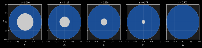
Figure 7: One-phase Stefan problem in the radially symmetric case ($d=2$). Evolution of the solid and the liquid regions over time.

Figure 8: Mean radius of the solid region over time (left panel) and zoomed in on the melting time (right panel). The light purple curves represent one standard deviation above and below the mean radius for various angles. The orange dashed curve is the theoretical melting rate from [16].

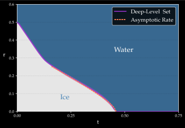
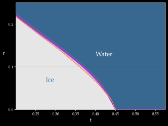
4.1.2 Two-phase, Freezing Regime $(d=2)$

Let $d=2$ and consider the two-phase, radially symmetric supercooled Stefan problem without surface tension. Suppose that the temperature is initially constant in the liquid and the solid regions, namely

$$u^{1}_{0}=-\frac{\mathds{1}_{B_{R}\setminus B_{r_{0}}}}{2|B_{R}\setminus B_{r_{0}}|},\qquad u^{2}_{0}=-\frac{1}{10|B_{r_{0}}|}\mathds{1}_{B_{r_{0}}}.$$

We therefore choose the constants $c_{1}=1/2,\ c_{2}=1/10$ in Remark 2. In this example, the radius of the solid region converges to some constant $r_{\infty}\in(0,R)$. In other words, the solid region neither melts completely nor covers the whole domain in the long run. In light of the Dirichlet condition (2e), the long-term temperature must be constant and equal to $u^{1}(\infty,\cdot)\equiv u^{2}(\infty,\cdot)\equiv 0$. In fact, the theoretical value for $r_{\infty}$ can be derived from the Stefan growth condition. Indeed, choosing an increasing sequence $\psi_{m}\in\operatorname{\mathcal{C}}^{\infty}_{c}(\Omega)$ such that $\psi_{m}\uparrow 1$ in $\Omega$ and time integrating (38) in the proof of Proposition 1 between $t=0-$ and $t=T\to\infty$ yields

$$|\Gamma_{\infty}|-|\Gamma_{0-}|=\frac{1}{L}\sum_{i=1}^{2}\bigg{(}\int_{\Gamma_{\infty}^{i}}u_{\infty}^{i}-\int_{\Gamma_{0-}^{i}}u_{0}^{i}\bigg{)}\;\Longleftrightarrow\;\pi r_{\infty}^{2}-\pi r_{0}^{2}=\frac{c_{1}+c_{2}}{L}.$$ (33)

The long-term radius is therefore $r_{\infty}=\sqrt{r_{0}^{2}+\frac{c_{1}+c_{2}}{L\pi}}$. We can thus solve for $r_{\infty}$ and compare it with the obtained long-term radius. We choose $r_{0}=1/2$, $L=4$, and $T=5$. The long-term radius is roughly equal to $0.59$, as confirmed in Fig. 9.

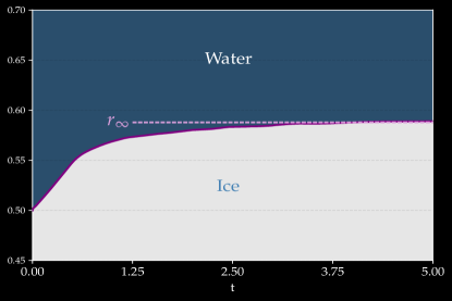
Figure 9: Two-phase, supercooled Stefan problem without surface tension ($d=2$) discussed in Section 4.1.2. The radius indeed converges to the theoretical long-term value $r_{\infty}\approx 0.59$.

Let us now estimate the temperature in both phases as a function of time and radius from the trained moving solid. In view of (5), we here have that $u^{i}(t,x)\,\mathrm{d}x=-c_{i}\operatorname{\mathbb{P}}(X_{t}^{i}\in\mathrm{d}x,\tau^{i}>t)$ for $t\in[0-,T]$, $i=1,2$. Writing $v^{i}(t,|x|)\mathrel{\mathop{\ordinarycolon}}=u^{i}(t,x)$ and using polar coordinates yields

$$v^{i}(t,r) =-\frac{c_{i}}{2\pi r}\underbrace{\frac{\operatorname{\mathbb{P}}(|X_{t}^{i}|\in\mathrm{d}r\ |\ \tau^{i}>t)}{\mathrm{d}r}}_{(a)}\ \underbrace{\operatorname{\mathbb{P}}(\tau^{i}>t)}_{(b)}.$$

The term $(a)$ is the time $t$ conditional density of the norm of surviving particles which can be approximated using Monte Carlo simulation and kernel density estimation (KDE). The second term $(b)$ is the unconditional survival probability over time and can also be estimated using simulation. Fig. 10 displays the temperature of the solid and the liquid over time. As can be seen, the temperature at time $t=2$ is already close to its equilibrium $u^{1}_{\infty}=u^{2}_{\infty}=0$.

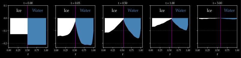
Figure 10: Two-phase, supercooled Stefan problem without surface tension ($d=2$) discussed in Section 4.1.2. Temperature (vertical axis) in the liquid ($u^{1}$) and the solid ($u^{2}$) retrieved using Monte Carlo simulation and kernel density estimation (KDE). At $t=3$, both phases are already close to their equilibrium temperature $u^{1}_{\infty}=u^{2}_{\infty}=0$ and long term term radius $r_{\infty}\approx 0.59$.

4.1.3 Two-phase, with Surface Tension $(d=3)$

Consider the three-dimensional Stefan problem with surface tension. The initial temperatures in the solid and the liquid are respectively given by

$$u^{1}_{0}=-\frac{\mathds{1}_{B_{R}\setminus B_{r_{0}}}}{2|B_{R}\setminus B_{r_{0}}|},\quad u^{2}_{0}=-\frac{\mathds{1}_{B_{r_{0}}}}{|B_{r_{0}}|}.$$

We therefore have $\eta=-1$ (supercooled liquid), $c_{1}=1/2$, and $c_{2}=1$. Again, the solution remains radially symmetric, i.e., $\Gamma_{t}=B_{r(t)}$ for some function $r\!\mathrel{\mathop{\ordinarycolon}}[0,T]\to[0,R]$. The temperature at the interface is therefore $u^{1}\equiv u^{2}\equiv-\frac{\gamma}{r(t)}$. We use the growth condition in Proposition 3 to train the parameters and estimate the mean curvature via Algorithm 3. To benchmark our method, we apply a useful trick in the three-dimensional radial case to get rid of surface tension. A similar argument is given in [19, Section 4]. For $i=1,2,$ define

$$\widetilde{u}^{i}(t,x)=u^{i}(t,x)+\frac{\gamma}{|x|}.$$ (34)

Then $\widetilde{u}^{1}\equiv\widetilde{u}^{2}\equiv 0$ on $\partial\Gamma$, so the Gibbs-Thomson condition (2e’) is effectively “absorbed” by the transformation in (34). In addition, $\Delta\left(|x|^{-1}\right)=(3-d)|x|^{-3}$, hence $x\mapsto|x|^{-1}$ is harmonic if $d=3$ and $\widetilde{u}^{i}$ still solves the heat equation (2a). We can therefore apply the deep level-set method without surface tension by changing the initial condition to $\widetilde{u}^{i}_{0}(x)=u^{i}_{0}(x)+\frac{\gamma}{|x|}$. It is worth noting that the Stefan condition (2d) is also affected. As $u^{i}=\widetilde{u}^{i}-\frac{\gamma}{|x|}$ and $\partial_{\nu}(\frac{1}{|x|})=-\frac{1}{|x|^{2}}$, we obtain

$$V=\frac{\alpha_{2}}{2L}\partial_{\nu}u^{2}-\frac{\alpha_{1}}{2L}\partial_{\nu}u^{1}=\frac{\alpha_{2}}{2L}\partial_{\nu}\widetilde{u}^{2}-\frac{\alpha_{1}}{2L}\partial_{\nu}\widetilde{u}^{1}+\gamma\frac{\alpha_{2}-\alpha_{1}}{2L|x|^{2}}.$$

If $\alpha_{1}=\alpha_{2}$, then the Stefan condition remains unchanged. Otherwise, when $t\mapsto r(t)$ is strictly monotone, the growth condition in (1) becomes

$$\int_{\Gamma_{0-}}\psi-\int_{\Gamma_{t}}\psi=\frac{1}{L}\Big{(}\operatorname{\mathbb{E}}^{\mu^{1}}[\psi(X_{\tau^{1}}^{1})\,\mathds{1}_{\{\tau^{1}\leq t\}}]-\operatorname{\mathbb{E}}^{\mu^{2}}[\psi(X_{\tau^{2}}^{2})\,\mathds{1}_{\{\tau^{2}\leq t\}}]+\operatorname{\mathcal{K}}_{t}\Big{)},\quad\psi\in\mathcal{C}_{c}^{\infty}(\Omega),$$

$$\operatorname{\mathcal{K}}_{t}=\gamma\frac{\alpha_{1}-\alpha_{2}}{2}\int_{0}^{t}\int_{\partial\Gamma_{s}}\frac{\psi}{|x|^{2}}=\gamma\frac{\alpha_{1}-\alpha_{2}}{2}\bigg{(}\int_{\Gamma_{t}}\frac{\psi}{|x|^{2}}-\int_{\Gamma_{0}}\frac{\psi}{|x|^{2}}\bigg{)}.$$

In this example, we assume that $\alpha_{1}=\alpha_{2}=\frac{1}{2}$, $L=2$, $\gamma=0.25$. The above remedy when $\alpha_{1}\neq\alpha_{2}$ is therefore not needed. We note that after the radial trick the liquid is still supercooled, i.e., $\widetilde{u}_{0}^{1}\leq 0$.

Fig. 11 compares the radius of the solid over time obtained from the growth condition in Proposition 3 (orange curve), using the radial trick (dashed purple curve), and without surface tension (red curve). The algorithm with surface tension and its benchmark indeed give similar results. As expected, the growth of the solid ball is less pronounced with surface tension as the freezing point becomes negative for convex solid regions.

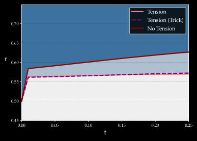
Figure 11: Two-phase, radially symmetric Stefan problem ($d=3$) with surface tension $(\gamma=0.25)$ and without. Time evolution of the radius of the solid obtained from the growth condition in Proposition 3 (orange curve), using the radial trick (dashed purple curve), and without surface tension (red curve).

4.1.4 Two-phase, Jump in the Radius $(d=2)$

Consider the two-dimensional radial supercooled Stefan problem inside the ball $\Omega=B_{1}\subseteq\operatorname{\mathbb{R}}^{2}$. We set the latent heat to $L=2$ and assume that there is no surface tension at the interface. Given $\Gamma_{0-}=B_{r_{0}}$, $r_{0}\in(0,R)$, and assuming the initial temperature to be radial, the solid region remains radial as well, i.e., $\Gamma_{t}=B_{r(t)}$ for some càdlàg function $[0-,T]\ni t\mapsto r(t)$. The goal of this experiment is to demonstrate the method’s ability to generate jumps in the radius $r(\cdot)$. To this end, consider the following initial condition:

$$u^{1}_{0}(x)=-\frac{1}{|A_{r_{0},\delta_{0}}|}\mathds{1}_{A_{r_{0},\delta_{0}}}(x),\quad u^{2}_{0}(x)=-\frac{1}{|B_{r_{0}}|}\mathds{1}_{B_{r_{0}}}(x),\quad A_{r_{0},\delta_{0}}=B_{r_{0}+\delta_{0}}\backslash B_{r_{0}},$$ (35)

where $r_{0}=\frac{1}{4},\ \delta_{0}=\frac{1}{8}$. In other words, the liquid is strongly supercooled inside the annulus $A_{r_{0},\delta_{0}}$ and at zero temperature elsewhere. We may therefore expect a sizeable liquid region surrounding the solid to freeze immediately, leading to an initial positive jump in the radius. This is indeed the case as observed in Fig. 13. As seen in Section 3.3, we can in fact quantify the magnitude of the jump for physical solutions. In this case, we have from (21) that $\Delta r(0)$ must be the smallest positive value (if any) such that

$$|A_{r_{0},\Delta}|=\frac{1}{L}\int_{A_{r_{0},\Delta}}\bigg{(}\!-\frac{\gamma}{|x|}-u^{1}_{0}(x)\!\bigg{)}.$$

Absent of surface tension ($\gamma=0$) and in light of the initial data in (35), this gives

$$|A_{r_{0},\Delta}|=\frac{1}{L}\int_{A_{r_{0},\Delta}}|u^{1}_{0}|\;\;\Longleftrightarrow\;\;\pi\big{(}(r_{0}+\Delta)^{2}-r_{0}^{2}\big{)}=\frac{(r_{0}+\Delta\wedge\delta_{0})^{2}-r_{0}^{2}}{L((r_{0}+\delta_{0})^{2}-r_{0}^{2})}.$$ (36)

Solving numerically, we obtain $\Delta r(0)\approx 0.22$. See also Fig. 12 which compares the area $|A_{r_{0},\Delta}|$ with the excess temperature $\frac{1}{L}\int_{A_{r_{0},\Delta}}|u^{1}_{0}|$ as functions of $\Delta$. We finally observe in Fig. 13 that the initial jump produced by the deep level-set method nearly matches the physical jump size.

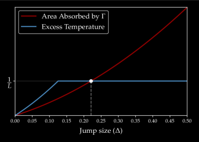
Figure 12: Magnitude of the jump in the radius obtained by equating the excess temperature (blue curve) to the volume absorbed (red curve), corresponding to the left-hand and the right-hand sides of (36), respectively. As can be seen, the initial jump size is roughly equal to $\Delta r(0)\approx 0.22$ (precisely $0.2208$).

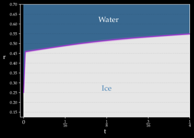
Figure 13: Two-dimensional, two-phase supercooled Stefan problem without surface tension. The initial jump has size $\approx 0.21$ (precisely $0.2098$) and is close to the physical jump $\Delta r(0)\approx 0.22$.

4.2 General Case

4.2.1 Two-phase, Square-shaped Solid ($d=2$)

Let $\Omega=B_{1}\subseteq\operatorname{\mathbb{R}}^{2}$ and suppose that $\Gamma_{0-}$ is the two-dimensional $\ell_{1}$-ball of radius $r_{0}\in(0,1)$. For the initial level-set function, we consider $\Phi_{0}(x)=|x|_{1}-r_{0}$, $|x|_{1}=\sum_{i=1}^{2}|x_{i}|$. The temperature is initially uniform in both the liquid and the solid, namely

$$u^{1}_{0}=-c_{1}\frac{\mathds{1}_{\Omega\setminus\Gamma_{0-}}}{|\Omega\setminus\Gamma_{0-}|},\quad u^{2}_{0}=-c_{2}\frac{\mathds{1}_{\Gamma_{0-}}}{|\Gamma_{0-}|}.$$

We choose $\ \alpha_{1}=1/2,\ \alpha_{2}=1/20$, $L=1/100$, and $\gamma=0$. This example intends to investigate the situation where the liquid particles have a much larger diffusivity than the solid particles. As the liquid is not supercooled, we expect the solid region to melt faster than with similar diffusivity.

As can be seen in Fig. 14, the solid region becomes rounder as the liquid particles are more likely to hit the corners of the initial square-shaped region. Moreover, the particles in the solid typically take longer to hit the interface as their diffusivity is far less than the one of the liquid particles.

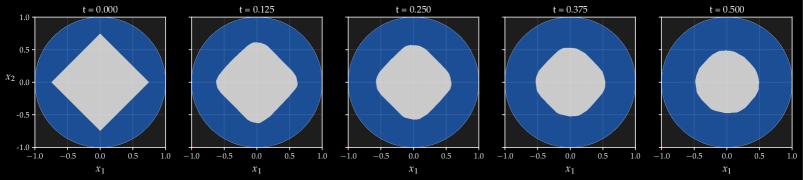
Figure 14: Two-phase Stefan problem with square-shaped initial solid region ($d=2$). Evolution of the solid over time (no surface tension).

Remark 7.

Recall that the neural network learns the difference between the level-set function $\Phi(t,\cdot)$, $t\in[0,T]$ and its initial value $\Phi_{0}(\cdot)$. However, $\Phi_{0}$ is not smooth in the following examples, so the lack of regularity will carry over to $\Phi(t,\cdot)$ for $t\in(0,T]$. To give more flexibility to the deep level-set function, one could consider

$$\Phi(t,x;\theta)\mathrel{\mathop{\ordinarycolon}}=G(t,x;\theta)+\Phi_{0}(x)(1-\widetilde{G}(t;\widetilde{\theta}))_{+},\quad t\in[0,T],$$

where $\widetilde{G}\!\mathrel{\mathop{\ordinarycolon}}[0,T]\times\widetilde{\Theta}\to\operatorname{\mathbb{R}}$ is another feedforward neural network taking only time as an input and capturing the decay of the initial level-set function. However, this additional flexibility did not prove helpful in our numerical experiments. One possible explanation is that the jump penalty prevents the auxiliary neural network from taking significant non-zero values.

4.2.2 Two-phase, Diamond-shaped Solid ($d=2$), Melting Regime

We are given a diamond-shaped solid $\Gamma_{0-}$ defined as the zero sublevel set of

$$\Phi_{0}(x)=\bigg{(}\sum_{i=1}^{2}|x_{i}|^{1/2}\bigg{)}^{2}-r_{0}.$$ (37)

See the leftmost panel of Fig. 15 for an illustration. We choose $r_{0}=3/4$ and the temperatures

$$u^{1}_{0}=\frac{\mathds{1}_{\Omega\setminus\Gamma_{0-}}}{|\Omega\setminus\Gamma_{0-}|},\qquad u^{2}_{0}=-\frac{\mathds{1}_{\Gamma_{0-}}}{4|\Gamma_{0-}|}.$$

We also set $\eta=1$, $L=1/4$, and $\gamma=0.15$. Fig. 15 displays the melting of the solid. As can be seen, the spikes of the diamond get rounder and it eventually becomes almost radially symmetric. This is because the liquid particles hit the interface more frequently near the spikes, having more contact points, which drives the melting process there.

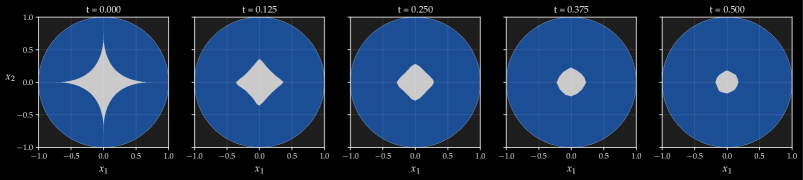
Figure 15: Two-phase Stefan problem with surface tension $(\gamma=0.15)$. Melting of a diamond-shaped solid region ($d=2$).

Figure 16: Two-phase Stefan problem with diamond-shaped initial solid region ($d=2$) and supercooled liquid. Evolution of the solid region over time.

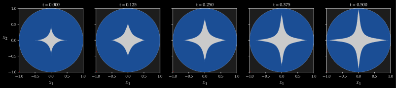
(a) Without surface tension.

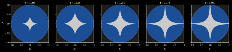
(b) With surface tension $(\gamma=0.15)$.

4.2.3 Two-phase, Diamond-shaped Solid ($d=2$), Freezing Regime

Consider as in Section 4.2.2 a diamond-shaped solid $\Gamma_{0-}$ with level-set function as in (37). The initial temperature is again uniform but the liquid is supercooled this time, namely

$$u^{1}_{0}=-c_{1}\frac{\mathds{1}_{\Omega\setminus\Gamma_{0-}}}{|\Omega\setminus\Gamma_{0-}|},\qquad u^{2}_{0}=-c_{2}\frac{\mathds{1}_{\Gamma_{0-}}}{|\Gamma_{0-}|}.$$

We choose $r_{0}=1/2$, $c_{1}=1$, $c_{2}=1/10$. The purpose of this example is to see the impact of surface tension on the growth of the solid. Recall from Remark 6 that for two-dimensional problems, only the sign of the curvature at the interface needs to be estimated (using Algorithm 2).

Figs. 16(a) and 16(b) show the evolution of the solid region for the surface tension coefficients $\gamma=0$ (no tension) and $\gamma=0.15$, respectively. Observe that the interface is strictly concave almost everywhere (except at the spikes). In light of the Gibbs-Thomson condition (2e’), the temperature at the boundary is above zero almost everywhere when surface tension is added, which accelerates the growth of the solid region. This is confirmed in Fig. 16(b).

4.2.4 Two-phase, Dumbbell-shaped Solid $(d=2)$

We finally investigate the melting of a dumbbell-shaped solid as in the top-left panel of Fig. 17. The following parameters are used:

$$\gamma=0.1,\quad c_{1}=2,\quad c_{2}=0.25,\quad\eta=1.$$

Again, the initial temperature is constant in both the liquid and the solid. As in the previous section, we use Algorithm 2 to determine the sign of the curvature along the boundary. Fig. 17 describes the short term evolution of the solid region. As can be seen, the solid disconnects in the time interval $[0.06,0.07]$. We also note that the middle of the “bar” melts faster than its extremities, namely the concave corners. Indeed, concave areas have a melting point above zero, which slows down the melting process.

Figure 17: Two-phase Stefan problem with surface tension and dumbbell-shaped solid region ($d=2$). The solid disconnects between $t=0.06$ and $t=0.07$.

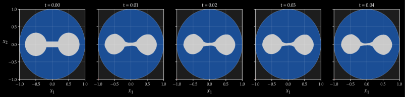
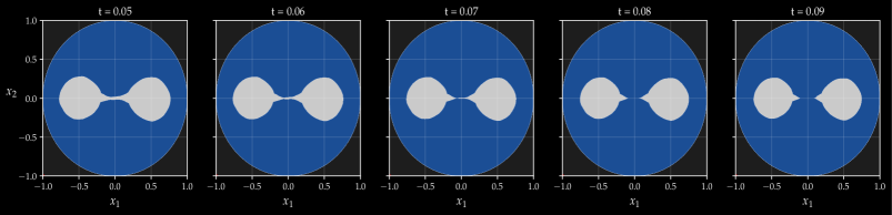
5 Conclusion

We combine the level-set method with deep learning to represent the solid region in two-phase Stefan problems. The growth condition of probabilistic solutions is turned into a loss function and estimated using Monte Carlo simulation. The parameters of the deep level-set function are then trained using a relaxed formulation. When adding surface tension, the algorithm involves the simulation of particles close to the solid-liquid interface and the computation of the mean curvature using a dilation technique. The latter only requires the outward normal vector to the boundary, which is readily available through automatic differentiation of the deep level-set function.

The numerical examples illustrate the validity and flexibility of the method. In the two-dimensional radial case, the algorithm is capable of accurately capturing known melting rates, long-term radius, and initial jumps in the radius. Further, the three-dimensional radial example of Section 4.1.3 accurately demonstrates the effect of surface tension. We subsequently apply the method to general examples in two dimensions, where the initial solid is square-, diamond-, or dumbbell-shaped. The effect of surface tension is also discussed.

We believe that our findings make a first step towards the computation and understanding of probabilistic solutions for general Stefan problems. Naturally, other examples can be explored. For instance, it would be interesting to see if the method can handle more complex dynamics with multiple jumps (e.g., Figure $1$ in [25]) or capture dendritic solidification [2, 14, 28]. Another direction of future research is to investigate non-radial three-dimensional examples, such as cubic or dumbbell-shaped solid regions.

More broadly, the deep level-set method can be applied to other free boundary problems as well, e.g., the Hele-Shaw and the Stokes flow [11]. In mathematical finance, the method can be adapted to describe the stopping region of American options, thus extending the “neural optimal stopping boundary method” [34] when the geometric structure of the exercise boundary is unknown. Another application would consist in computing the no-trade zone in portfolio choice problems with transaction costs [24].

Appendix A Proofs

A.1 Proposition 1

Proof.

Let $(u^{1},u^{2},\Gamma)$ be a classical solution of (2a) $\!-$(2e). Without loss of generality, we prove the claim for $\eta=1$. First, the Stefan condition and the divergence theorem give

$$L\ \frac{\mathrm{d}}{\mathrm{d}t}\int_{\Gamma_{t}}\psi =L\int_{\partial\Gamma_{t}}V\psi$$

$$=\frac{\alpha_{2}}{2}\int_{\partial\Gamma_{t}}\partial_{\nu}u^{2}\ \psi-\frac{\alpha_{1}}{2}\int_{\partial\Gamma_{t}}\partial_{\nu}u^{1}\ \psi$$

$$=\sum_{i=1}^{2}\frac{\alpha_{i}}{2}\int_{\Gamma_{t}^{i}}\text{div}(\nabla u^{i}\ \psi)$$

$$=\sum_{i=1}^{2}\frac{\alpha_{i}}{2}\int_{\Gamma_{t}^{i}}(\Delta u^{i}\ \psi+\nabla u^{i}\cdot\nabla\psi).$$

Observing that the velocity of $\Gamma^{1}_{t}$ is $-V$, we obtain

$$\int_{\Gamma_{t}^{i}}\frac{\alpha_{i}}{2}\Delta u^{i}\psi=\int_{\Gamma_{t}^{i}}\partial_{t}u^{i}\ \psi=\frac{\mathrm{d}}{\mathrm{d}t}\int_{\Gamma_{t}^{i}}u^{i}\psi-(-1)^{i}\int_{\partial\Gamma_{t}^{i}}Vu^{i}\psi.$$

In light of the Dirichlet boundary condition (2e), the last (surface) integral vanishes. Moreover, integration by parts gives

$$\frac{\alpha_{i}}{2}\int_{\Gamma_{t}^{i}}\nabla u^{i}\cdot\nabla\psi=(-1)^{i}\frac{\alpha_{i}}{2}\int_{\partial\Gamma_{t}^{i}}u^{i}\partial_{\nu}\psi-\frac{\alpha_{i}}{2}\int_{\Gamma_{t}^{i}}u^{i}\Delta\psi=-\frac{\alpha_{i}}{2}\int_{\Gamma_{t}^{i}}u^{i}\Delta\psi,$$

invoking again the Dirichlet boundary condition. Thus,

$$L\ \frac{\mathrm{d}}{\mathrm{d}t}\int_{\Gamma_{t}}\psi=\sum_{i=1}^{2}\bigg{(}\frac{\mathrm{d}}{\mathrm{d}t}\int_{\Gamma_{t}^{i}}u^{i}\psi-\frac{\alpha_{i}}{2}\int_{\Gamma_{t}^{i}}u^{i}\Delta\psi\bigg{)}.$$ (38)

For $t\geq 0$, define $\overleftarrow{\;\tau}^{i}_{t}=\inf\{s\geq 0\!\mathrel{\mathop{\ordinarycolon}}X_{0}^{i}+\sqrt{\alpha_{i}}\ W^{i}_{s}+l^{i}_{s}\notin\Gamma^{i}_{t-s}\}$. Note that, by a Feynman-Kac formula,

$$u^{i}(t,x)=\operatorname{\mathbb{E}}^{\operatorname{\mathbb{P}}_{x}}[u_{0}^{i}(X_{t}^{i})\,\mathds{1}_{\{\overleftarrow{\;\tau}^{i}_{t}>t\}}],\quad x\in\Gamma_{t}^{i},$$

where the subscript in $\operatorname{\mathbb{P}}_{x}$ indicates that $X_{0}^{i}=x$. Using the time reversibility of Brownian motion, Itô’s formula and the definition of $\tau^{i}$ in (3), we obtain

$$(-1)^{i+1}\int_{\Gamma_{t}^{i}}u^{i}\psi =\int_{\Gamma_{t}^{i}}\operatorname{\mathbb{E}}^{\operatorname{\mathbb{P}}_{x}}[|u_{0}^{i}(X_{t}^{i})|\,\mathds{1}_{\{\overleftarrow{\;\tau}^{i}_{t}>t\}}]\ \psi(x)\,\mathrm{d}x$$

$$=\int_{\Gamma_{t}^{i}}\int_{\Gamma_{0}^{i}}|u_{0}^{i}(y)|\operatorname{\mathbb{P}}_{x}(X_{t}^{i}\in\mathrm{d}y,\overleftarrow{\;\tau}^{i}_{t}>t)\ \psi(x)\,\mathrm{d}x$$

$$=\int_{\Gamma_{0}^{i}}\int_{\Gamma_{t}^{i}}\psi(x)\operatorname{\mathbb{P}}_{y}(X_{t}^{i}\in\mathrm{d}x,\tau^{i}>t)\ |u_{0}^{i}(y)|\,\mathrm{d}y\$$

$$=\operatorname{\mathbb{E}}^{\mu^{i}}[\psi(X_{t}^{i})\,\mathds{1}_{\{\tau^{i}>t\}}]\hskip 142.26378pt$$

$$=\operatorname{\mathbb{E}}^{\mu^{i}}[\psi(X_{\tau^{i}\wedge t}^{i})]-\operatorname{\mathbb{E}}^{\mu^{i}}[\psi(X_{\tau^{i}}^{i})\,\mathds{1}_{\{\tau^{i}\leq t\}}]$$

$$=\operatorname{\mathbb{E}}^{\mu^{i}}[\psi(X^{i}_{0})]+\frac{\alpha_{i}}{2}\int_{0}^{t}\underbrace{\operatorname{\mathbb{E}}^{\mu^{i}}[\Delta\psi(X_{s}^{i})\,\mathds{1}_{\{\tau^{i}>s\}}]}_{=(-1)^{i+1}\int_{\Gamma_{s}^{i}}u^{i}\Delta\psi}\,\mathrm{d}s-\operatorname{\mathbb{E}}^{\mu^{i}}[\psi(X_{\tau^{i}}^{i})\,\mathds{1}_{\{\tau^{i}\leq t\}}].$$

Hence $\frac{\mathrm{d}}{\mathrm{d}t}\int_{\Gamma_{t}^{i}}u^{i}\psi-\frac{\alpha_{i}}{2}\int_{\Gamma_{t}^{i}}u^{i}\Delta\psi=(-1)^{i}\frac{\mathrm{d}}{\mathrm{d}t}\operatorname{\mathbb{E}}^{\mu^{i}}[\psi(X_{\tau^{i}}^{i})\,\mathds{1}_{\{\tau^{i}\leq t\}}]$ and the result follows.

∎

A.2 Proposition 2

Proof.

It is enough to prove the claim for $\eta=1$. Looking at the proof of Proposition 1 and using that $u^{1},u^{2}$ coincide on $\partial\Gamma$, we gather that

$$L\ \frac{\mathrm{d}}{\mathrm{d}t}\int_{\Gamma_{t}}\psi =\sum_{i=1}^{2}\bigg{(}\frac{\mathrm{d}}{\mathrm{d}t}\int_{\Gamma_{t}^{i}}u^{i}\psi-(-1)^{i}\int_{\partial\Gamma_{t}}Vu^{i}\psi+\frac{\alpha_{i}}{2}\int_{\Gamma_{t}^{i}}\nabla u^{i}\cdot\nabla\psi\bigg{)}$$

$$=\sum_{i=1}^{2}\bigg{(}\frac{\mathrm{d}}{\mathrm{d}t}\int_{\Gamma_{t}^{i}}u^{i}\psi-\frac{\alpha_{i}}{2}\int_{\Gamma_{t}^{i}}u^{i}\Delta\psi\bigg{)}-\dot{\operatorname{\mathcal{K}}}_{t}^{I},$$

where $\dot{\operatorname{\mathcal{K}}}_{t}^{I}\ =\gamma\frac{\alpha_{2}-\alpha_{1}}{2}\int_{\partial\Gamma_{t}}\kappa_{\partial\Gamma_{t}}\ \partial_{\nu}\psi$. Moreover, $u^{i}$ admits the Feynman-Kac representation

$$u^{i}(t,x)=\operatorname{\mathbb{E}}^{\operatorname{\mathbb{P}}_{x}}[u_{0}^{i}(X_{t}^{i})\,\mathds{1}_{\{\overleftarrow{\;\tau}^{i}_{t}>t\}}]-\gamma K^{i}(t,x),\quad x\in\Gamma_{t}^{i},$$

with $K^{i}$ and $\overleftarrow{\;\tau}^{i}_{t}$ given in the statement. This implies that

$$L\ \frac{\mathrm{d}}{\mathrm{d}t}\int_{\Gamma_{t}}\psi=\sum_{i=1}^{2}(-1)^{i}\frac{\mathrm{d}}{\mathrm{d}t}\operatorname{\mathbb{E}}^{\mu^{i}}[\psi(X_{\tau^{i}}^{i})\,\mathds{1}_{\{\tau^{i}\leq t\}}]\ -\dot{\operatorname{\mathcal{K}}}_{t}^{I}-\dot{\operatorname{\mathcal{K}}}_{t}^{II}+\dot{\operatorname{\mathcal{K}}}_{t}^{III},$$

with the additional terms

$$\dot{\operatorname{\mathcal{K}}}_{t}^{II}\ =\gamma\sum_{i=1}^{2}\frac{\mathrm{d}}{\mathrm{d}t}\int_{\Gamma_{t}^{i}}K^{i}\psi,\quad\dot{\operatorname{\mathcal{K}}}_{t}^{III}\ =\gamma\sum_{i=1}^{2}\frac{\alpha_{i}}{2}\int_{\Gamma_{t}^{i}}K^{i}\Delta\psi.$$ (39)

Next, due to (10), $K^{i}$ is a weak solution of the heat equation in any rectangle $\operatorname{\mathcal{R}}\subseteq\text{int}\ \Gamma^{i}$, i.e.,

$$\int_{\operatorname{\mathcal{R}}}\Big{(}\partial_{t}+\frac{\alpha_{i}}{2}\Delta\Big{)}\psi\ K^{i}=0,\quad\psi\in\operatorname{\mathcal{C}}_{c}^{\infty}(\operatorname{\mathcal{R}}).$$

From Weyl’s Lemma, we conclude that $K^{i}$ is in fact a strong solution of $\partial_{t}K^{i}=\frac{\alpha_{i}}{2}\Delta K^{i}$ in $\text{int}\ \Gamma^{i}$. Noting also that $K^{1}=K^{2}$ on $\partial\Gamma$, we have

$$\frac{1}{\gamma}\dot{\operatorname{\mathcal{K}}}_{t}^{II}\ =\sum_{i=1}^{2}\frac{\mathrm{d}}{\mathrm{d}t}\int_{\Gamma_{t}^{i}}K^{i}\psi=\sum_{i=1}^{2}\bigg{(}\int_{\Gamma_{t}^{i}}\partial_{t}K^{i}\ \psi+(-1)^{i}\int_{\partial\Gamma_{t}}VK^{i}\psi\bigg{)}=\sum_{i=1}^{2}\int_{\Gamma_{t}^{i}}\frac{\alpha_{i}}{2}\Delta K^{i}\ \psi.$$

Using Green’s second identity, note that (again, the outward normal of $\Gamma_{t}^{1}$ is $-\nu$)

$$\int_{\Gamma_{t}^{i}}\Delta K^{i}\ \psi=(-1)^{i}\int_{\partial\Gamma_{t}}(\partial_{\nu}K^{i}\ \psi-K^{i}\ \partial_{\nu}\psi)+\int_{\Gamma_{t}^{i}}K^{i}\Delta\psi.$$

Given the definition of $\dot{\operatorname{\mathcal{K}}}_{t}^{III}$ in (39) and recalling that $K^{1}|_{\partial\Gamma}=K^{2}|_{\partial\Gamma}=\kappa_{\partial\Gamma}$, this implies that

$$\dot{\operatorname{\mathcal{K}}}_{t}^{II}-\dot{\operatorname{\mathcal{K}}}_{t}^{III} =\gamma\sum_{i=1}^{2}(-1)^{i}\frac{\alpha_{i}}{2}\int_{\partial\Gamma_{t}}(\partial_{\nu}K^{i}\ \psi-\kappa_{\partial\Gamma_{t}}\ \partial_{\nu}\psi)$$

$$=-\dot{\operatorname{\mathcal{K}}}_{t}^{I}+\gamma\int_{\partial\Gamma_{t}}\bigg{(}\frac{\alpha_{2}}{2}\partial_{\nu}K^{2}-\frac{\alpha_{1}}{2}\partial_{\nu}K^{1}\bigg{)}\psi$$

$$=-\dot{\operatorname{\mathcal{K}}}_{t}^{I}+\frac{\mathrm{d}}{\mathrm{d}t}\operatorname{\mathcal{K}}_{t}.$$

Integrating in time and rearranging yields the claim. ∎

A.3 Proposition 3

Proof.

Assume again that $\eta=1$. Using similar arguments to the ones in the proof of Proposition 1, we can show that

$$L\bigg{(}\int_{\Gamma_{0-}}\psi-\int_{\Gamma_{t}}\psi\bigg{)} =\sum_{i=1}^{2}\bigg{(}\int_{\Gamma_{0-}^{i}}u^{i}\psi-\int_{\Gamma_{t}^{i}}u^{i}\psi+\frac{\alpha_{i}}{2}\int_{0}^{t}\int_{\Gamma_{s}^{i}}u^{i}\Delta\psi\bigg{)}.$$ (40)

Expressing $u\mathrel{\mathop{\ordinarycolon}}=-u^{1}\,\mathds{1}_{\Gamma_{t}^{1}}-u^{2}\,\mathds{1}_{\Gamma_{t}^{2}}$ via [25, Lemma 2.4], we find for $\varphi\in\{\psi,\Delta\psi\}$,

$$(-1)^{i+1}\int_{\Gamma_{t}^{i}}u^{i}\varphi =\operatorname{\mathbb{E}}[\varphi(X_{t}^{i})\,\mathds{1}_{\{\tau^{i}>t\}}]+(-1)^{i}\ \lim_{\delta\downarrow 0}\ \operatorname{\mathbb{E}}\bigg{[}\sum_{l=1}^{\infty}\varphi(Y_{t}^{l,i})\,\mathds{1}_{\{T_{l}^{\delta,i}\leq t<\tau^{\delta,i}_{l}\}}\bigg{]}.$$ (41)

Next, let us temporarily write $(Y,T_{l},\tau_{l},\alpha)=(Y^{l,i},T_{l}^{\delta,i},\tau_{l}^{\delta,i},\alpha_{i})$ to simplify notation. Using Itô’s lemma and Fubini’s theorem, observe that

$$\psi(Y_{t})\,\mathds{1}_{\{T_{l}\leq t<\tau_{l}\}} =\psi(Y_{\tau_{l}\wedge t})\,\mathds{1}_{\{T_{l}\leq t\}}-\psi(Y_{\tau_{l}})\,\mathds{1}_{\{\tau_{l}\leq t\}}$$

$$=\psi(Y_{T_{l}})\,\mathds{1}_{\{T_{l}\leq t\}}+\frac{\alpha}{2}\int_{0}^{t}\Delta\psi(Y_{s})\,\mathds{1}_{\{T_{l}\leq s<\tau_{l}\}}\,\mathrm{d}s$$

$$\quad+\int_{T_{l}\wedge t}^{\tau_{l}\wedge t}\nabla\psi(Y_{s})\cdot\mathrm{d}Y_{s}-\psi(Y_{\tau_{l}})\,\mathds{1}_{\{\tau_{l}\leq t\}}$$

$$\Longrightarrow\;\;\operatorname{\mathbb{E}}[\psi(Y_{t})\,\mathds{1}_{\{T_{l}\leq t<\tau_{l}\}}] =\operatorname{\mathbb{E}}[\psi(Y_{T_{l}})\,\mathds{1}_{\{T_{l}\leq t\}}-\psi(Y_{\tau_{l}})\,\mathds{1}_{\{\tau_{l}\leq t\}}]+\frac{\alpha}{2}\int_{0}^{t}\operatorname{\mathbb{E}}[\Delta\psi(Y_{s})\,\mathds{1}_{\{T_{l}\leq s<\tau_{l}\}}]\,\mathrm{d}s.$$

Similarly, for $X_{t}^{i}$ and $\tau^{i}$, we have

$$\operatorname{\mathbb{E}}[\psi(X_{t}^{i})\,\mathds{1}_{\{\tau^{i}>t\}}] =\operatorname{\mathbb{E}}[\psi(X_{0}^{i})-\psi(X_{\tau^{i}}^{i})\,\mathds{1}_{\{\tau^{i}\leq t\}}]\ +\frac{\alpha_{i}}{2}\int_{0}^{t}\operatorname{\mathbb{E}}[\Delta\psi(X_{s}^{i})\,\mathds{1}_{\{\tau^{i}>s\}}]\,\mathrm{d}s.$$

Plugging the above expressions into (41), with $\varphi=\psi$, and invoking Fubini’s theorem, we obtain

$$(-1)^{i+1}\bigg{(}\int_{\Gamma_{0-}^{i}}u^{i}\psi-\int_{\Gamma_{t}^{i}}u^{i}\psi\bigg{)} =-\frac{\alpha_{i}}{2}\int_{0}^{t}\operatorname{\mathbb{E}}[\Delta\psi(X_{s}^{i})\,\mathds{1}_{\{\tau^{i}>s\}}]\,\mathrm{d}s+\operatorname{\mathbb{E}}[\psi(X_{\tau^{i}}^{i})\,\mathds{1}_{\{\tau^{i}\leq t\}}]$$

$$\quad-(-1)^{i}\ \lim_{\delta\downarrow 0}\ \operatorname{\mathbb{E}}\bigg{[}\sum_{l=1}^{\infty}\Big{(}\psi(Y_{T_{l}^{\delta,i}}^{l,i})\,\mathds{1}_{\{T_{l}^{\delta,i}\leq t\}}-\psi(Y_{\tau_{l}^{\delta,i}}^{l,i})\,\mathds{1}_{\{\tau^{\delta,i}_{l}\leq t\}}\Big{)}\bigg{]}$$

$$\quad-(-1)^{i}\ \lim_{\delta\downarrow 0}\ \frac{\alpha_{i}}{2}\int_{0}^{t}\operatorname{\mathbb{E}}\bigg{[}\sum_{l=1}^{\infty}\Delta\psi(Y_{s}^{l,i})\,\mathds{1}_{\{T_{l}^{\delta,i}\leq s<\tau^{\delta,i}_{l}\}}\bigg{]}\,\mathrm{d}s$$

$$=(-1)^{i}\ \frac{\alpha_{i}}{2}\int_{0}^{t}\int_{\Gamma_{s}^{i}}u^{i}\Delta\psi\ \,\mathrm{d}s+\operatorname{\mathbb{E}}[\psi(X_{\tau^{i}}^{i})\,\mathds{1}_{\{\tau^{i}\leq t\}}]+(-1)^{i}\operatorname{\mathcal{K}}_{t}^{i},$$

using (41) with $\varphi=\Delta\psi$ for the last equality. In view of (40) and the definition of $\operatorname{\mathcal{K}}$, $(N^{\delta,i})_{i=1}^{2}$ in the statement, we indeed find that

$$\int_{\Gamma_{0-}}\psi-\int_{\Gamma_{t}}\psi =\frac{1}{L}\Big{(}\operatorname{\mathbb{E}}^{\mu^{1}}[\psi(X_{\tau^{1}}^{1})\,\mathds{1}_{\{\tau^{1}\leq t\}}]-\operatorname{\mathbb{E}}^{\mu^{2}}[\psi(X_{\tau^{2}}^{2})\,\mathds{1}_{\{\tau^{2}\leq t\}}]+\operatorname{\mathcal{K}}_{t}\Big{)}.$$

∎

References

- Alessandri et al. [2019] A. Alessandri, P. Bagnerini, and M. Gaggero. Optimal control of propagating fronts by using level set methods and neural approximations. IEEE Transactions on Neural Networks and Learning Systems, 30(3):902–912, 2019.
- Almgren [1993] R. Almgren. Variational algorithms and pattern formation in dendritic solidification. Journal of Computational Physics, 106(2):337–354, 1993.
- Ambrosio and Soner [1996] L. Ambrosio and H. M. Soner. Level set approach to mean curvature flow in arbitrary codimension. Journal of Differential Geometry, 43(4):693–737, 1996.
- Bachouch et al. [2022] A. Bachouch, C. Huré, N. Langrené, and H. Pham. Deep Neural Networks Algorithms for Stochastic Control Problems on Finite Horizon: Numerical Applications. Methodology and Computing in Applied Probability, 24(1):143–178, 2022.
- Barles et al. [1993] G. Barles, H. M. Soner, and P. E. Souganidis. Front propagation and phase field theory. SIAM Journal on Control and Optimization, 31(2):439–469, 1993.
- Becker et al. [2019] S. Becker, P. Cheridito, and A. Jentzen. Deep optimal stopping. Journal of Machine Learning Research, (74):1–25, 2019.
- Becker et al. [2021] S. Becker, P. Cheridito, A. Jentzen, and T. Welti. Solving high-dimensional optimal stopping problems using deep learning. European Journal of Applied Mathematics, 32(3):470–514, 2021.
- Boettinger et al. [2002] W. J. Boettinger, J. A. Warren, C. Beckermann, and A. Karma. Phase-field simulation of solidification. Annual Review of Materials Research, 32(1):163–194, 2002.
- Chen et al. [1997] S. Chen, B. Merriman, S. Osher, and P. Smereka. A simple level set method for solving Stefan problems. Journal of Computational Physics, 135(1):8–29, 1997.
- Cuchiero et al. [2023] C. Cuchiero, S. Rigger, and S. Svaluto-Ferro. Propagation of minimality in the supercooled Stefan problem. The Annals of Applied Probability, 33(2):1588 – 1618, 2023.
- Cummings et al. [1999] L. J. Cummings, S. D. Howison, and J. R. King. Two-dimensional Stokes and Hele-Shaw flows with free surfaces. European Journal of Applied Mathematics, 10(6):635–680, 1999.
- Delarue et al. [2022] F. Delarue, S. Nadtochiy, and M. Shkolnikov. Global solutions to the supercooled Stefan problem with blow-ups: regularity and uniqueness. Probability and Mathematical Physics, 3(1):171–213, 2022.
- Figalli [2018] A. Figalli. Regularity of interfaces in phase transitions via obstacle problems. Proceedings of the International Congress of Mathematicians, 2018.
- Gibou et al. [2002] F. Gibou, R. Fedkiw, R. Caflisch, and S. Osher. A level set approach for the numerical simulation of dendritic growth. Journal of Scientific Computing, 19, 2002.
- Guo et al. [2023] Y. Guo, S. Nadtochiy, and M. Shkolnikov. Stefan problem with surface tension: uniqueness of physical solutions under radial symmetry. arXiv:2306.02969, 2023.
- Hadzic and Raphael [2015] M. Hadzic and P. Raphael. On melting and freezing for the 2D radial Stefan problem. Journal of the European Mathematical Society, 21, 2015.
- Han and E [2016] J. Han and W. E. Deep learning approximation for stochastic control problems. NIPS, 2016.
- Han et al. [2018] J. Han, A. Jentzen, and W. E. Solving high-dimensional partial differential equations using deep learning. Proceedings of the National Academy of Sciences, 115(34):8505–8510, 2018.
- Herraiz et al. [2001] L. A. Herraiz, M. A. Herrero, and J. J. L. Velázquez. A note on the dissolution of spherical crystals. Proceedings of the Royal Society of Edinburgh: Section A Mathematics, 131(2):371–389, 2001.
- Kingma and Ba [2015] D. P. Kingma and J. Ba. Adam: a method for stochastic optimization. Proceedings of the International Conference on Learning Representations (ICLR), 2015.
- Lamé and Clapeyron [1831] G. Lamé and B. P. Clapeyron. Mémoire sur la solidification par réfroidissement d’un globe liquide. Ann. Chimie Physique, 47:250–256, 1831.
- Luckhaus [1990] S. Luckhaus. Solutions for the two-phase Stefan problem with the Gibbs–Thomson law for the melting temperature. European Journal of Applied Mathematics, 1(2):101–111, 1990.
- Mescheder et al. [2018] L. M. Mescheder, M. Oechsle, M. Niemeyer, S. Nowozin, and A. Geiger. Occupancy networks: Learning 3d reconstruction in function space. 2019 IEEE/CVF Conference on Computer Vision and Pattern Recognition (CVPR), pages 4455–4465, 2018.
- Muhle-Karbe et al. [2017] J. Muhle-Karbe, M. Reppen, and H. M. Soner. A primer on portfolio choice with small transaction costs. Annual Review of Financial Economics, 9(1):301–331, 2017.
- Nadtochiy and Shkolnikov [2022] S. Nadtochiy and M. Shkolnikov. Stefan problem with surface tension: global existence of physical solutions under radial symmetry. arXiv:2203.15113, 2022.
- Nadtochiy et al. [2021] S. Nadtochiy, M. Shkolnikov, and X. Zhang. Scaling limits of external multi-particle DLA on the plane and the supercooled Stefan problem. arXiv:2102.09040, 2021.
- Osher and Sethian [1988] S. Osher and J. A. Sethian. Fronts propagating with curvature-dependent speed: Algorithms based on Hamilton-Jacobi formulations. Journal of Computational Physics, 79(1):12–49, 1988.
- Osher and Fedkiw [2003] S. J. Osher and R. Fedkiw. Level set methods and dynamic implicit surfaces, volume 153 of Applied mathematical sciences. Springer, 2003.
- Park et al. [2019] J. J. Park, P. R. Florence, J. Straub, R. A. Newcombe, and S. Lovegrove. Deepsdf: Learning continuous signed distance functions for shape representation. 2019 IEEE/CVF Conference on Computer Vision and Pattern Recognition (CVPR), pages 165–174, 2019.
- Pham et al. [2021] H. Pham, X. Warin, and M. Germain. Neural networks-based backward scheme for fully nonlinear PDEs. SN Partial Differential Equations and Applications, 2, 2021.
- Popinet [2018] S. Popinet. Numerical models of surface tension. Annual Review of Fluid Mechanics, 50(1):49–75, 2018.
- Raissi et al. [2019] M. Raissi, P. Perdikaris, and G. Karniadakis. Physics-informed neural networks: A deep learning framework for solving forward and inverse problems involving nonlinear partial differential equations. Journal of Computational Physics, 378:686–707, 2019.
- Reppen et al. [2022a] A. M. Reppen, H. M. Soner, and V. Tissot-Daguette. Deep stochastic optimization in finance. Digital Finance, 2022a.
- Reppen et al. [2022b] A. M. Reppen, H. M. Soner, and V. Tissot-Daguette. Neural optimal stopping boundary. arXiv:2205.04595, 2022b.
- Sethian [1999] J. A. Sethian. Level Set Methods and Fast Marching Methods: Evolving Interfaces in Computational Geometry, Fluid Mechanics, Computer Vision, and Materials Science. Cambridge Monographs on Applied and Computational Mathematics. Cambridge University Press, 1999.
- Sirignano and Spiliopoulos [2018] J. Sirignano and K. Spiliopoulos. Dgm: A deep learning algorithm for solving partial differential equations. Journal of Computational Physics, 375:1339–1364, 2018.
- Soner [1993] H. M. Soner. Motion of a set by the curvature of its boundary. Journal of Differential Equations, 101(2):313–372, 1993.
- Soner [1995] H. M. Soner. Convergence of the phase-field equations to the Mullins-Sekerka problem with kinetic undercooling. Archive for Rational Mechanics and Analysis, 131(2):139–197, 1995.
- Soner and Tissot-Daguette [2023] H. M. Soner and V. Tissot-Daguette. Stopping times of boundaries: Relaxation and continuity. arXiv:2305.09766, 2023.
- Stefan [1889] J. Stefan. Über einige Probleme der Theorie der Wärmeleitung. Sitzungsberichte der Kaiserlichen Akademie der Wissenschaften in Wien – mathematisch-naturwissenschaftliche Classe, 98:473–484, 1889.
- Stefan [1890a] J. Stefan. Über die Theorie der Eisbildung. Monatshefte für Mathematik und Physik, 1(1):1–6, 1890a.
- Stefan [1890b] J. Stefan. Über die Verdampfung und die Auflösung als Vorgänge der Diffusion. Annalen der Physik, 277:725–747, 1890b.
- Stefan [1891] J. Stefan. Über die Theorie der Eisbildung, insbesondere über die Eisbildung im Polarmeere. Annalen der Physik und Chemie, 42:269–286, 1891.
- Visintin [1989] A. Visintin. Stefan problem with surface tension. In Mathematical Models for Phase Change Problems, pages 191–213. Springer, 1989.
- Wang and Perdikaris [2021] S. Wang and P. Perdikaris. Deep learning of free boundary and Stefan problems. Journal of Computational Physics, 428:109914, 2021.
- Wang et al. [2021] S. Wang, Y. Teng, and P. Perdikaris. Understanding and mitigating gradient flow pathologies in physics-informed neural networks. SIAM Journal on Scientific Computing, 43(5):A3055–A3081, 2021.