Quantum decoherence of free electrons and interaction with distant objects

Abstract

Quantum physics rules the dynamics of small objects as they interact over microscopic length scales. Nevertheless, quantum correlations involving macroscopic distances can be observed between entangled photons as well as in atomic gases and matter waves at low temperatures. The long-range nature of the electromagnetic coupling between charged particles and extended objects could also trigger quantum phenomena over large distances. Here, we reveal a manifestation of quantum mechanics that involves macroscopic distances and results in a nearly complete depletion of coherence associated with which-way free-electron interference produced by electron–radiation coupling in the presence of a distant extended object. We illustrate this effect by a rigorous theoretical analysis of a two-path electron beam interacting with a semi-infinite plate and find the inter-path coherence to vanish proportionally to the path separation at zero temperature and exponentially at finite temperature. Besides the fundamental interest of this macroscopic quantum phenomenon, our results suggest an approach to measuring the vacuum temperature and nondestructively sensing the presence of distant objects.

I Introduction

The wave nature of electrons allows us to image materials with atomic resolution in transmission electron microscopy Egerton (2005); Muller et al. (2008) (TEM) and resolve the atomic structure and dynamics of molecules and crystal surfaces through low-energy C.Davisson and Germer (1927); Pendry (1974), photoemission Rehr et al. (2002), and ultrafast Wolter et al. (2016); Filippetto et al. (2022) electron diffraction. In these techniques, wave interference takes place between elastically scattered components, while inelastic collisions are typically regarded as a source of decoherence that destroys interference through the addition of a stochastic phase.

Decoherence can be produced by coupling to material excitations. In particular, an electron split into two paths and moving parallel to a lossy planar surface was proposed Anglin et al. (1997), extensively studied from a theoretical viewpoint Anglin et al. (1997); Mazzitelli et al. (2003); Levinson (2004); Hsiang and Lee (2006); Machnikowski (2006); Howie (2011); Scheel and Buhmann (2012), and experimentally confirmed Sonnentag and Hasselbach (2007); Hasselbach (2010); Beierle et al. (2018); Kerker et al. (2020); Chen and Batelaan (2020) to be a suitable configuration to observe electron decoherence. In a related scenario, inelastic electron scattering produced by coupling to thermally populated low-energy material excitations was shown to render an observable loss of electron coherence that limits spatial resolution in TEM Uhlemann et al. (2013, 2015).

Electron decoherence is equally produced by inelastic excitations associated with photon emission and electromagnetic vacuum fluctuations, as predicted for an electron prepared in a prescribed two-path configuration Ford (1993, 1997), including the effect of neighboring perfect-conductor boundaries Ford (1993); Mazzitelli et al. (2003); Hsiang and Lee (2006). Likewise, radiative electron decoherence is anticipated to take place due to bremsstrahlung emission Breuer and Petruccione (2001), interaction with time-varying fields Hsiang and Ford (2004), and the Smith-Purcell effect Alvarez and Mazzitelli (2008). Intriguingly, recoherence can occur for electrons moving in a squeezed vacuum Hsiang and Ford (2008).

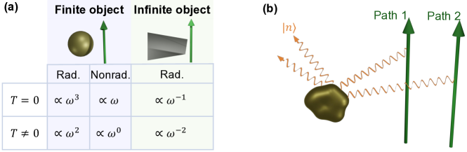
Figure 1: Infrared divergences in e-beam decoherence. (a) Low-frequency scaling of the spectrally resolved probability for a beamed electron to undergo radiative inelastic scattering and lose an energy quantum $\hbar\omega$ during the interaction with finite and extended structures. The latter are represented by an infinite wedge. We also show the scaling for nonradiative scattering by a lossy finite object for comparison. (b) Illustration of decoherence for an e-beam split into two paths, arising from the differences in the scattering amplitude associated with each of the electron paths when exciting modes $n$ (e.g., photons in radiative scattering).

Surprisingly, the probability that a moving electron undergoes inelastic energy exchanges when passing near an extended material structure can diverge in common structures due to the contribution of low-energy radiative modes García de Abajo (2009). This result is in apparent contradiction with the preservation of coherence in off-axis electron holography Lehmann and Lichte (2002); Winkler et al. (2018), which relies on interference between electrons passing either through or outside a material to reconstruct its atomic structure. Therefore, the question arises, is a divergent excitation probability compatible with the observation of electron interference phenomena? Analysis of the spectrally resolved excitation probability $\Gamma(\omega)$ reveals a divergence as $\propto 1/\omega$ for small exchanged energies $\hbar\omega$ at zero temperature in many common geometries García de Abajo (2009). The results summarized in Fig. 1a show that a divergence is found when coupling to extended material structures, while the response of finite objects vanishes in the $\omega\to 0$ limit. In addition, at finite temperature $T$, the probability associated with the coupling to bosonic modes (e.g., photons and polaritons) must be multiplied by a factor $n_{T}(\omega)+1$ for electron energy losses ($\omega>0$) and $n_{T}(-\omega)$ for gains ($\omega<0$) García de Abajo and Di Giulio (2021), where $n_{T}(\omega)=({\rm e}^{\hbar\omega/{k_{\rm B}}T}-1)^{-1}$ is the Bose-Einstein distribution function, which also scales as $\propto 1/\omega$ at low frequencies. Consequently, we expect an overall divergence as $\Gamma(\omega)\propto 1/\omega^{2}$ at finite temperature. Reassuringly, the average electron energy loss [i.e., the frequency integral of $\hbar\omega\,\Gamma(\omega)$] remains finite and temperature-independent because $n_{T}$ terms cancel when adding losses and gains.

Interesting insight into decoherence is provided by the fact that energy-filtered inelastically scattered electrons are observed to undergo interference in TEM after spatially separate electron components excite extended excitation modes such as plasmons Lichte and Freitag (2000); Herring (2005); Verbeeck et al. (2008). Considering a two-path electron (i.e., a wave function split into two non-overlapping spatial components $1$ and $2$, see Fig. 1b), scattering by a structure initially prepared in the ground state $\ket{n=0}$ produces an overall post-interaction state $\sum_{n}\big{(}a_{n}\ket{n}\otimes\ket{1}+b_{n}\ket{n}\otimes\ket{2}\big{)}$, where $n$ runs over excited states of the structure. In an interference experiment that mixes both paths at a detector, the electron count rate exhibits oscillations as a function of scattering angle with an amplitude $\propto\sum_{n}{\rm Re}\{a_{n}b_{n}^{*}\}$. A certain degree of coherence is then preserved if paths $1$ and $2$ can both excite each given mode $n$ with nonvanishing amplitudes, just like in a quantum eraser Zeilinger (1999); Ma et al. (2016) that produces a loss of which-way information.

Quantum-mechanical effects taking place over macroscopic distances have so far been observed by leveraging the lossless propagation of photons in free space Horodecki et al. (2009); Togan et al. (2010) or by preparing superposition matter states at low temperatures Monroe et al. (1996); Brune et al. (1996). As a genuinely quantum-mechanical effect, decoherence may potentially be produced at macroscopic electron-path separations when photons play the role of the inelastic modes $\ket{n}$ in the analysis above. Such an effect could benefit from the aforementioned infrared divergences, which favor coupling to long-wavelength radiative modes. We thus pose the question of whether electron decoherence can be switched on and off by placing an object at a macroscopic distance from a broad electron beam, thus resulting in the manifestation of a macroscopic quantum effect (i.e., involving large electron–object separations) taking place at finite (e.g., room) temperatures.

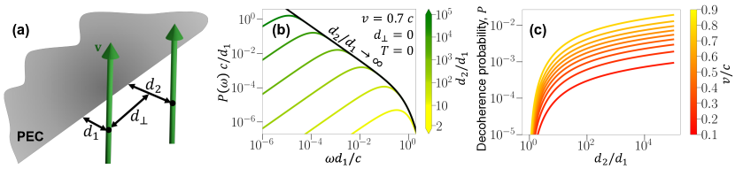
Figure 2: Two-path decoherence by a half-plane at zero temperature. (a) System under consideration, consisting of a single electron split into a two-path spatial superposition and passing close and perpendicularly to a perfectly conducting half-plane at distances $d_{1}$ and $d_{2}$ from the edge [beam path positions ${\bf R}_{1}=(0,d_{1})$ and ${\bf R}_{2}=(d_{\perp},d_{2})$]. (b) Universal plot of the spectrally resolved decoherence probability for various $d_{2}/d_{1}$ ratios (color curves) with $d_{\perp}=0$, approaching a divergent profile in the $d_{2}\gg d_{1}$ limit (black curve). We consider an electron velocity $v=0.9\,c$ and normalize the frequency and the probability using the smallest distance $d_{1}$. (c) Decoherence probability as a function of $d_{2}/d_{1}$ for $d_{\perp}=0$ and different electron velocities (see color scale).

Here, we theoretically demonstrate that the presence of an extended material structure can produce strong electron decoherence on electron beams placed at an arbitrarily large distance from the material. We consider radiative modes of commensurably large wavelengths, for which the materials behave either as real-permittivity dielectrics or lossless perfect electric conductors (PECs). Specifically, we consider a PEC thin half-plane and a two-path electron beam passing perpendicularly to it (Fig. 2a). Because the half-plane in the zero-thickness limit is a scale-invariant structure and the PEC response eliminates any absolute length scale from the problem at zero temperature, we find that the decoherence between the two paths only depends on the ratio of their distances to the half-plane, and consequently, decoherence is predicted to take place for arbitrarily large macroscopic electron–half-plane distances, provided the inter-path separation is sufficiently large. At finite vacuum temperature $T$, the thermal wavelength $\lambda_{T}=2\pi\hbar c/{k_{\rm B}}T$ plays a role by imposing an absolute length scale that is inversely proportional to $T$ (e.g., $\lambda_{T}\sim 14\,$mm at 1 K and 50 $\mu$m at room temperature). We find that decoherence is then boosted for large inter-path separations compared with $\lambda_{T}$, provided one of the paths passes near the half-plane. In a more practical scenario, we consider a finite-width ribbon and show that the half-plane limit is recovered for large width compared with the electron–edge distance. Our results support the use of electron decoherence to sense the presence of distant objects and measure the vacuum temperature.

II General theory of electron-beam decoherence

We are interested in investigating the loss of coherence among different spatial regions of a single electron prepared in a beam moving along $z$ with velocity $v$. The electron state can change due to the interaction with the environment (i.e., any material structure and the radiation field), giving rise to inelastic components that are position-dependent and, thus, decreasing the degree of coherence between separate spatial regions of the beam. As a practical manifestation of this effect, after propagation from those regions to an electron detector, the loss of coherence produces a reduction in the visibility of the resulting interference fringes, which we investigate here in a rigorous quantitative manner.

Describing an incident electron through its interaction-picture density matrix $\rho_{e}^{i}({\bf r},{\bf r}^{\prime})$, scattering by a structure produces a final density matrix given by

$$\rho_{e}^{f}({\bf r},{\bf r}^{\prime})={\rm e}^{-P({\bf r},{\bf r}^{\prime})+{\rm i}\chi({\bf r},{\bf r}^{\prime})}\rho_{e}^{i}({\bf r},{\bf r}^{\prime}),$$ (1)

where

$$P({\bf R},{\bf R}^{\prime}) =\frac{1}{2}\int_{0}^{\infty}d\omega\big{[}2n_{T}(\omega)+1\big{]}$$ (2)

$$\times\bigg{[}\Gamma({\bf R},{\bf R},\omega)+\Gamma({\bf R}^{\prime},{\bf R}^{\prime},\omega)-2\Gamma({\bf R},{\bf R}^{\prime},\omega)\bigg{]}$$

is the decoherence probability, which is in turn expressed as a frequency integral of the generalized loss probability

$$\Gamma({\bf R},{\bf R}^{\prime},\omega)=\frac{4e^{2}}{\hbar}\int_{-\infty}^{\infty}dz \int_{-\infty}^{\infty}dz^{\prime}\cos\Big{[}\frac{\omega}{v}(z-z^{\prime})\Big{]}$$ (3)

$$\times{\rm Im}\{-G_{zz}({\bf r},{\bf r}^{\prime},\omega)\}.$$

(a self-contained derivation of these expressions is presented in Appendices A and B). The scattering structure enters this formalism through the electromagnetic Green tensor $G({\bf r},{\bf r}^{\prime},\omega)$, which can be calculated by solving the macroscopic electromagnetic response according to Eq. (B19). The real phase $\chi({\bf r},{\bf r}^{\prime})$ in Eq. (1) is also expressed in terms of the Green function (see Appendix B), adding a rigid shift to the fringes observed in two-path interference. As anticipated above, the effect of temperature is encapsulated in the Bose-Einstein distribution function $n_{T}(\omega)$. Following pioneering studies of decoherence in free-space electrons Ford (1993), explicit results analogous to these expressions have been obtained by using macroscopic quantum electrodynamics Scheel and Buhmann (2012); Di Giulio and García de Abajo (2020), but the derivation that we present in Appendices A and B is self-contained and formulated in more general terms.

Electron decoherence by a half-plane

The application of Eqs. (2) and (3) to an electron beam passing outside and perpendicularly to a PEC half-plane produces analytical expressions for the decoherence probability, as shown in the self-contained derivation offered in Appendix C. More precisely, referring to the geometry depicted in Fig. 2a, involving two paths with transverse coordinates ${\bf R}_{1}=(d_{1},0)$ and ${\bf R}_{2}=(d_{2},d_{\perp})$, we find

$$P({\bf R}_{1},{\bf R}_{2})= \frac{\alpha}{2\pi}\int_{0}^{1}d\mu\;\frac{\big{[}2\mu^{2}+\eta^{2}\big{]}\,\sqrt{1-\mu^{2}}}{\big{[}\mu^{2}+\eta^{2}\big{]}^{3/2}}\int_{0}^{\infty}\frac{d\theta}{\theta}\;\coth(\theta/4\pi)$$ (4)

$$\times\bigg{\{}{\rm e}^{-2\theta\,(d_{1}/\lambda_{T})\sqrt{\mu^{2}+\eta^{2}}}+{\rm e}^{-2\theta\,(d_{2}/\lambda_{T})\sqrt{\mu^{2}+\eta^{2}}}-2\cos\big{[}\mu\theta\,d_{\perp}/\lambda_{T}\big{]}\,{\rm e}^{-\theta\,[(d_{1}+d_{2})/\lambda_{T}]\sqrt{\mu^{2}+\eta^{2}}}\bigg{\}},$$

where $\alpha=e^{2}/\hbar c\approx 1/137$ is the fine structure constant and $\eta=c/v\gamma$ is a velocity-dependent parameter that uses the relativistic Lorentz factor $\gamma=1/\sqrt{1-v^{2}/c^{2}}$. The integration variable $\theta=2\pi\hbar\omega/{k_{\rm B}}T$ in Eq. (4) encapsulates the exchanged energy $\hbar\omega$, and we have rewritten the thermal factor as

$$2n_{T}(\omega)+1=\coth(\theta/4\pi).$$ (5)

As we argue above, this factor and $\Gamma({\bf R},{\bf R}^{\prime},\omega)$ are both diverging as $1/\omega$ in the $\omega\to 0$ limit. However, the divergence is canceled because the expression inside curly brackets in Eq. (4) behaves as $\propto\theta^{2}\sim\omega^{2}$ for small $\omega$: the first two terms inside the curly brackets represent the contributions arising from the two separate electron paths passing by ${\bf R}_{1}$ and ${\bf R}_{2}$, respectively, whereas the rightmost term stands for path interference, and while the integral of each of these three terms diverges, their sum becomes finite. Consequently, the decoherence probability $P({\bf R}_{1},{\bf R}_{2})$ remains finite. We note that this quantity vanishes for ${\bf R}_{1}={\bf R}_{2}$, as expected from Eq. (2), and it depends on ${\bf R}_{1}$, ${\bf R}_{2}$, and $T$ only through the ratios $d_{1}/\lambda_{T}$, $d_{2}/\lambda_{T}$, and $d_{\perp}/\lambda_{T}$.

II.1 Zero-temperature limit

In the zero-temperature limit, we have $n_{T}(\omega)\to 0$, so we can approximate $\coth(\theta/4\pi)\approx 1$ in Eq. (4) [see Eq. (5)]. The $\theta$ integral can then be performed analytically by first absorbing the $(1/\lambda_{T})\sqrt{\mu^{2}+\eta^{2}}$ factor of the exponentials into the integration variable, and then considering the identity $\int_{0}^{\infty}d\theta\,{\rm e}^{-a\sqrt{\theta^{2}+g^{2}}}/\sqrt{\theta^{2}+g^{2}}=K_{0}(ga)$ (see Eq. 3.914-4 in Ref. Gradshteyn and Ryzhik (2007)) together with the expansion $K_{0}(ga)=\log(2)-\log(ga)-\mathcal{C}+\mathcal{O}[(ga)^{2}\log(ga)]$ for $ga\ll 1$, where $\mathcal{C}$ is the Euler constant. Applying this result to the three terms inside the curly brackets of Eq. (4), setting $d_{\perp}=0$, and taking the $g\to 0$ limit, we find the result

$$P_{T=0}(d_{1},d_{2},d_{\perp}=0)=\frac{\alpha}{2\pi}\,f(v/c)\,\log\!\bigg{[}\frac{(d_{1}+d_{2})^{2}}{4d_{1}d_{2}}\bigg{]},$$ (6)

where $f(v/c)=\int_{0}^{1}d\mu\;\big{[}2\mu^{2}+\eta^{2}\big{]}$ $\sqrt{1-\mu^{2}}\;\big{[}\mu^{2}+\eta^{2}\big{]}^{-3/2}$ encapsulates the dependence on electron velocity via the variable $\eta=c/v\gamma$. Incidentally, this function admits the closed-form expression $f(\beta)=(\beta\gamma)^{-1}\big{\{}(2\gamma^{2}+1)\,\mathcal{K}(-\beta^{2}\gamma^{2})-3\mathcal{E}(-\beta^{2}\gamma^{2})\big{\}}$ in terms of the elliptical integrals $\mathcal{K}$ and $\mathcal{E}$. Interestingly, the dependences on path positions and electron velocity are factorized in Eq. (6). The distance dependence of the decoherence probability exhibits a logarithmic divergence as $P(d_{1},d_{2})\approx(\alpha/2\pi)\,f(v/c)\,|\!\log(d_{2}/d_{1})|$ in the $d_{2}/d_{1}\to 0,\infty$ limits, while it vanishes for $d_{1}=d_{2}$. In addition, $P(d_{1},d_{2})$ vanishes at $v=0$ and diverges as $\propto\log\gamma$ as the electron velocity approaches the speed of light.

It is instructive to examine the frequency integral of Eq. (4) in the $T=0$ limit. For $d_{\perp}=0$ and $d_{2}>d_{1}$, Fig. 2b shows that low frequencies become increasingly relevant as we increase $d_{2}$, eventually converging to a profile that diverges as $\propto 1/\omega$ at low frequencies in the $d_{2}/d_{1}\rightarrow\infty$ limit, for which the frequency integral is consequently infinite (i.e., we have full decoherence preventing any interference when mixing the two paths).

Universal curves for the decoherence probability are obtained from Eq. (6) for $d_{\perp}=0$ as a function of $d_{2}/d_{1}$ (Fig. 2c) for different electron velocities. Despite the logarithmic divergence with $d_{2}/d_{1}$ and the $\propto\log\gamma$ divergence as $v$ approaches $c$, the decoherence probability takes relatively small values at $T=0$ within the wide range of distances and velocities explored in Fig. 2c. This conclusion is however dramatically changed at finite temperatures, as we show below.

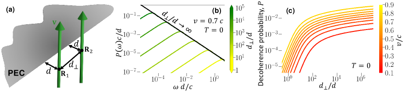
Figure S1: Two-path decoherence by a half-plane at zero temperature for laterally displaced paths. (a) System under consideration, consisting of a single electron split into a two-path spatial superposition and passing close and perpendicularly to a perfectly conducting half-plane at a distance $d$ from the edge with a lateral separation $d_{\perp}$ [beam path positions ${\bf R}_{1}=(0,d)$ and ${\bf R}_{2}=(d_{\perp},d)$]. (b) Universal plot of the spectrally resolved decoherence probability for various $d_{\perp}/d$ ratios (color curves), approaching a divergent profile in the $d_{\perp}\gg d$ limit (black curve). We consider an electron velocity $v=0.7\,c$ and normalize the frequency and the probability using the distance $d$. (c) Decoherence probability as a function of $d_{\perp}/d$ for different electron velocities (see color scale).

Similar results as those presented in Fig. 2b,c are obtained for the zero-temperature decoherence probability when varying the inter-path distance $d_{\perp}$ along the direction parallel to the half-plane edge while setting $d_{1}=d_{2}$ (see Fig. S1 in the Supplemental Material EPA ), which we calculate by numerically integrating Eq. (4) after setting $\coth(\theta/4\pi)=1$.

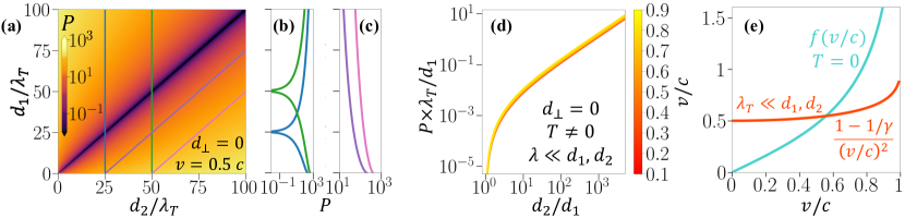
Figure 3: Decoherence at finite temperature. (a) Decoherence probability under the two-path configuration of Fig. 2a as a function of path-edge distances $d_{1}$ and $d_{2}$, normalized to the thermal wavelength $\lambda_{T}=2\pi c\hbar/{k_{\rm B}}T$. We set the electron velocity to $v=0.5\,c$. (b,c) Cuts of the probability in (a) along the color-coordinated lines. (d) Decoherence probability in the high-temperature limit ($d_{1},d_{2}\gg\lambda_{T}$), in which $\lambda_{T}P/d_{1}$ is only a function of $d_{2}/d_{1}$. (e) Electron-velocity prefactors in the $T=0$ and $d_{1},d_{2}\gg\lambda_{T}$ limits. We set $d_{\perp}=0$ in all cases.

II.2 Decoherence at finite temperature

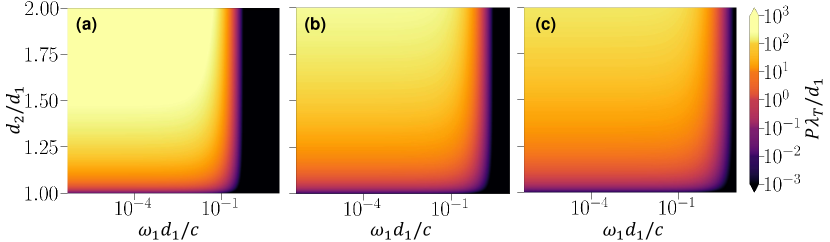
Figure S2: Spectral decomposition of the decoherence probability by a half-plane at finite temperature. We consider the configuration of Fig. 2a in the main text with $d_{\perp}=0$ and present results for three different electron velocities in panels (a)-(c) (see labels).

We examine the full dependence of the decoherence probability $P$ [Eq. (4)] on $d_{1}/\lambda_{T}$ and $d_{2}/\lambda_{T}$ for $d_{\perp}=0$ in Fig. 3a-c, setting $v/c=0.5$ as an illustrative example, since the dependence on velocity is relatively mild (see also Fig. S2 in the Supplemental Material EPA ). The diagonal of the plot in Fig. 3a is dominated by a depletion of the decoherence probability when $|d_{1}-d_{2}|\lesssim\lambda_{T}$ (see also Fig. 3b). However, $P$ quickly rises to large values when the distance difference is a few times the thermal wavelength (Fig. 3c).

It is interesting to analytically examine the high-temperature limit, in which the integral in Eq. (4) is dominated by regions where $n_{T}(\omega)\approx{k_{\rm B}}T/\hbar\omega\gg 1$ [see Eq. (B18)], so we can approximate $\coth(\theta/4\pi)\approx 4\pi/\theta$ [see Eq. (5)]. Setting again $d_{\perp}=0$, and changing the $\theta$ variable of integration to absorb the $(1/\lambda_{T})\sqrt{\mu^{2}+\eta^{2}}$ factor, the $\theta$ integral can be analytically performed by using the identity $\int_{0}^{\infty}d\theta\,{\rm e}^{-a\theta}/(\theta^{2}+g^{2})=(1/g)[{\rm Ci}(ga)\sin(ga)-{\rm Si}(ga)\cos(ga)]$ (see Eq. 3.354-1 in Ref. Gradshteyn and Ryzhik (2007)), where ${\rm Ci}$ and ${\rm Si}$ are the cosine and sine integral functions, respectively. We then expand ${\rm Ci}(ga)=\mathcal{C}+\log(ga)+\mathcal{O}(ga)^{2}$ and ${\rm Si}(ga)=-\pi/2+ga+\mathcal{O}(ga)^{2}$ for $ga\ll 1$, and from here, we find $\int_{0}^{\infty}d\theta\,{\rm e}^{-a\theta}/(\theta^{2}+g^{2})\approx a\log a+\cdots$, where the eliminated terms are linear in $a$, independent of $a$, or vanishing in the $g\to 0$ limit, so they do not contribute to the $\theta$ integral when summing the three exponential terms in Eq. (4). The $\mu$ integral of the remaining $a\log a$ contribution can also be performed in closed form, leading to the final result

$$P_{d_{1},d_{2}\gg\lambda_{T}} (d_{1},d_{2},d_{\perp}=0)=\frac{\alpha}{2}\,\frac{(1-1/\gamma)}{(v/c)^{2}}$$ (7)

$$\times\bigg{[}\frac{d_{1}}{\lambda_{T}}\log\Big{(}\frac{2d_{1}}{d_{1}+d_{2}}\Big{)}+\frac{d_{2}}{\lambda_{T}}\log\Big{(}\frac{2d_{2}}{d_{1}+d_{2}}\Big{)}\bigg{]},$$

where we again observe a factorization of the dependences on electron–half-plane distances and electron velocity. The decoherence probability $P$ exhibits a linear divergence with $d_{1}$ and $d_{2}$ for a constant ratio $d_{2}/d_{1}$ in the $d_{1},d_{2}\gg\lambda_{T}$ limit. In addition, the temperature enters through an overall factor $1/\lambda_{T}={k_{\rm B}}T/2\pi\hbar c\propto T$, so that $P$ also scales linearly with $T$.

In the high-temperature limit [Eq. (7)], the scaled probability $\lambda_{T}P/d_{1}$ only depends on the ratios $d_{2}/d_{1}$ and $v/c$, and in particular, it exhibits a roughly linear increase with $d_{2}/d_{1}$, as shown in Fig. 3d. We further observe the noted linear scaling with $T$, directly reflecting the linear increase with temperature in the photon population at long photon wavelengths (i.e., those that are commensurate with the electron–edge distances, which are large compared with $\lambda_{T}$ in the limit under examination). In addition, the dependence on electron velocity is fully contained in the prefactor $0.5\leq(1-1/\gamma)/(v/c)^{2}<1$ in Eq. (7), which takes finite values over a broad range of velocities typically used in electron microscopes, down to $v=0$ (Fig. 3e). This is in contrast to the $T=0$ behavior, in which, although $P$ also depends on velocity through a prefactor $f(v/c)$ [see Eq. (6)], the latter vanishes in the small velocity limit.

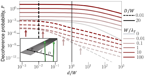
Figure 4: Finite size effects on the decoherence probability. We plot the decoherence probability $P$ for the system sketched in the lower-left inset. The electron beam is prepared in a two-path superposition state (inter-path distance $D$) and interacts with a thin metallic ribbon of width $W$. The path-ribbon distances are $d$ and $d+D$. We present results for different values of the $D/W$ and $W/\lambda_{T}$ ratios (see the legend on the right).

III Finite-size effects: decoherence by a metallic ribbon

While the assumption of a thin PEC screen is reasonable for metallic films of small thickness compared with the electron–edge distances, a finite extension of the half-plane geometry can play a role because the aforementioned infrared divergence requires that the structure to responds at arbitrarily low frequencies (see Fig. 1a). We study finite-size effects by limiting the extension of the half-plane in one direction and considering instead a ribbon of finite width $W$. The decoherence probability is then computed by employing an ad hoc boundary-element method in which the ribbon is discretized through a uniform set of points along the transverse direction, as explained in the self-contained Appendix D.

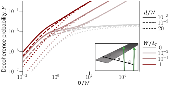
Figure S3: Finite size effects on the decoherence probability. Similar to Fig. 4 in the main text, but with the decoherence probability $P$ plotted as a function of the inter-path separation $D$ normalized to the ribbon width $W$. The electron beam is prepared in a two-path superposition state (inter-path distance $D$) and interacts with a ribbon of width $W$. The path–ribbon distances are $d$ and $d+D$. We present results for different values of the $d/W$ and $W/\lambda_{T}$ ratios (see the legend on the right).

The resulting decoherence probability is plotted in Fig. 4 for a two-path configuration featuring an inter-path distance $D$ and a shortest electron–ribbon distance $d$ (see inset). (See also Fig. S3 in the Supplemental Material EPA .) Specifically, we show results for $D/W=0.01$ and 20, combined with different $W/\lambda_{T}$ ratios ranging from zero temperature to $W=\lambda_{T}$. At large inter-path separations ($D=20\,W$, solid curves), the infinite half-plane limit is recovered for distances $d\ll W$. The condition $d=W$ (vertical solid line) signals the transition between the half-plane limit and a regime in which the probability is exponentially attenuated when increasing $d$ at all temperatures. This behavior is produced by ribbon-mediated coupling of the path that is closest to the edge to radiative modes, while the distant path experiences a negligible degree of inelastic interaction.

For relatively small inter-path separations ($D=0.01\,W$, dashed curves in Fig. 4), both paths undergo a similar level of inelastic interaction, and consequently, $P$ is strongly reduced compared to the results for large $D$. Under these conditions, the half-plane limit is recovered at $d\sim D=0.01\,W$ (vertical dashed line) in both the low- and high-temperature regimes ($W/\lambda_{T}=0$ and $\gg 1$, respectively). Similarly to the half-plane, a departure from the $T=0$ regime is observed at large ribbon–electron separations, as indicated by color-coordinated vertical arrows in Fig. 4. At large temperatures, this departure takes place over the entire range of distances $d$ considered in the figure, thus producing an overall increase in the decoherence probability.

IV CONCLUSIONS

In summary, inelastic radiative scattering of free electrons passing near extended structures produces a divergence in electron decoherence at high temperatures and/or large inter-path separations for electrons prepared in a two-path beam configuration. In essence, the material structure acts as a coupler between the evanescent electron field and free-space radiation. We exemplify this effect through an analytical treatment of the interaction between free electrons and a metallic half-plane, which is a self-scaling geometry such that, at zero temperature, there are no absolute length scales in the system, and therefore, the decoherence probability only depends on the ratio of electron-path distances to the edge. The decoherence probability increases with temperature as we depart from $T=0$. Then, the thermal wavelength defines an absolute length scale in the system. These results require the involvement of low-frequency radiation, with wavelengths that are commensurate with both the electron-path–edge distances and the extension of the material, as confirmed by the observation that the half-plane limit is recovered when considering instead ribbons of large width compared with the thermal wavelength and the electron–edge distance.

These results suggest the possibility of detecting the presence of distant objects without perturbing them (i.e., without causing any inelastic excitation in the involved materials, and relying instead on decoherence produced by coupling to radiative modes). Indeed, at zero temperature, the self-scaling nature of the half-plane geometry implies that a large decoherence probability is produced for any arbitrarily large electron–edge distance, provided the latter is small compared with the inter-path separation. In addition, at finite temperatures, a high degree of decoherence is observed when the inter-path distance is large compared with the thermal wavelength.

The strong temperature dependence of the decoherence probability could be exploited to perform vacuum thermometry and measure the temperature of the free-space thermal radiation bath. The required inter-path distances are a few times the thermal wavelength. At room temperature, the latter is $\lambda_{T}\approx 50\,\mu$m, so we need to consider distances of hundreds of microns, which are typical separations between electron beams and different structural components in electron microscopes. Incidentally, some degree of undesired electron decoherence could be produced due to radiative coupling assisted by elements placed close to the electron beam in electron microscopes, an effect that deserves further examination in light of the results presented in this work.

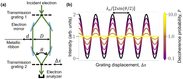
Figure S4: A possible configuration for measuring electron decoherence with large inter-path separations. (a) Electron optics scheme incorporating a transmission grating that splits the incident beam into two paths; two upper electrostatic mirrors that redirect the paths such they run parallel to each other with a separation $D$ at the position of the specimen (e.g., a wide metallic ribbon); two subsequent mirrors that make the paths converge; a second movable transmission grating that mixes the two paths into a single Bragg transmission direction; and an electron detector. The second grating must have a period $\lambda_{e}/\sin(\theta/2)$ determined by the angle $\theta$ between the two convergent paths and the electron wavelength $\lambda_{e}$, such that Bragg scattering combines both of them along a direction normal to the grating. The electron signal oscillates with the lateral displacement of the grating $\Delta x$, provided the two paths maintain some degree of coherence. (b) Interference pattern as a function of grating 2 displacement $\Delta x$ for different values of the decoherence probability produced by radiative coupling mediated by the ribbon under the configuration of (a), showing an interference pattern with period $\lambda_{e}/[2\sin(\theta/2)]$. Gratings similar to those used in previous studies Johnson et al. (2021, 2022) would fit in the current scheme.

Our predictions could therefore be tested in an electron microscope by introducing a specimen consisting of a wide ribbon (e.g., having width $W=20\,\lambda_{T}\approx 1\,$mm at room temperature) and splitting the electron beam into two paths (e.g., separated by a distance $D=W$). Then, interference between the two paths is significantly reduced when bringing the ribbon within a distance $d<0.1\,W\approx 0.1\,$mm from the nearest electron path (e.g., $P>0.2$). We further conceive a macroscopic version of this experiment at cryogenic temperatures, for which the decoherence probability is preserved if all lengths are scaled by the thermal wavelength (e.g., multiplied by a factor of $\sim 100$ when moving from room temperature to outer-space thermal-background conditions at 2.7 K). The far-field interference arising when mixing electron paths that are separated by a distance $D$ results in interference fringes with an angular spacing $\propto 1/D$, which becomes too small to be experimentally resolved at macroscopic separations $D$ of hundreds of microns. Instead, an electron optics system could be used to split an electron beam and separate the electron paths to the desired distance $D$ in the region of interaction with the material structure, followed by a second set of optical components that bring the electron paths to interference at the post-selecting transmission grating Johnson et al. (2021, 2022) (see Fig. S4 in the Supplemental Material EPA ).

The $1/r$ distance dependence of the electromagnetic fields produced by a moving charge (the electron) underscores the observed divergences in electron decoherence. An analogous divergence in decoherence could potentially be produced by other types of excitations that share similar long-range behavior. In particular, further investigation is needed to explore the effect of coupling between massive particle waves and gravitons, as well as the gravitational interaction with long-range modes in material structures (e.g., sound and elastic waves).

Appendix A General description of electron-beam decoherence

Starting from the Dirac equation to describe the electron and the radiation field, working in an electromagnetic gauge with zero scalar potential (the so-called temporal gauge), neglecting ponderomotive interactions, and adopting the nonrecoil approximation (i.e., considering an electron of high kinetic energy $E_{0}$ and constant electron velocity ${\bf v}$ under the assumption of small momentum exchanges with the environment compared with the initial electron momentum $\hbar{\bf q}_{0}$), one finds the approximate real-space Hamiltonian $\hat{\mathcal{H}}({\bf r})=\hat{\mathcal{H}}_{\rm rad}+\hat{\mathcal{H}}_{\rm el}({\bf r})+\hat{\mathcal{H}}_{\rm int}({\bf r})$, where $\hat{\mathcal{H}}_{\rm rad}$ and $\hat{\mathcal{H}}_{\rm el}({\bf r})=E_{0}-\hbar{\bf v}\cdot{\bf q}_{0}-{\rm i}\hbar{\bf v}\cdot\nabla$ describe the noninteracting radiation and electron components, while $\hat{\mathcal{H}}_{\rm int}({\bf r})=(e{\bf v}/c)\cdot\hat{\bf A}({\bf r})$ is the minimal-coupling radiation–electron interaction, which is simply proportional to the vector potential operator $\hat{\bf A}({\bf r})$ (see Ref. Di Giulio et al. (2019) for a detailed derivation starting from the Dirac equation). It is useful to move to the interaction picture, in which the interaction Hamiltonian becomes

$$\hat{\mathcal{H}}_{\rm int}({\bf r},t) ={\rm e}^{{\rm i}[\hat{\mathcal{H}}_{\rm rad}+\hat{\mathcal{H}}_{\rm el}({\bf r})]t/\hbar}\,\hat{\mathcal{H}}_{\rm int}({\bf r})\,{\rm e}^{-{\rm i}[\hat{\mathcal{H}}_{\rm rad}+\hat{\mathcal{H}}_{\rm el}({\bf r})]t/\hbar}$$

$$=\frac{e{\bf v}}{c}\cdot\hat{\bf A}({\bf r}+{\bf v}t,t),$$ (A8)

where $\hat{\bf A}({\bf r})$ inside $\hat{\mathcal{H}}_{\rm int}({\bf r})$ acquires a time dependence from both the transformation $\hat{\bf A}({\bf r},t)={\rm e}^{{\rm i}\hat{\mathcal{H}}_{\rm rad}t/\hbar}\hat{\bf A}({\bf r}){\rm e}^{-{\rm i}\hat{\mathcal{H}}_{\rm rad}t/\hbar}$ and the displacement introduced by the $-{\rm i}\hbar{\bf v}\cdot\nabla$ term in $\hat{\mathcal{H}}_{\rm el}$ [i.e., we apply the identity not (a) ${\rm e}^{{\bf v}t\cdot\nabla}f({\bf r}){\rm e}^{-{\bf v}t\cdot\nabla}g({\bf r})=f({\bf r}+{\bf v}t)g({\bf r})$, which is valid for any ${\bf r}$-dependent functions $f({\bf r})$ and $g({\bf r})$].

It is convenient to describe the temporal dynamics through the evolution operator $\hat{\mathcal{S}}({\bf r},t)$, defined in such a way that the combined electron–environment state at time $t$ is given by $\ket{\psi({\bf r},t)}=\hat{\mathcal{S}}({\bf r},t)\ket{\psi({\bf r},-\infty)}$, where $\ket{\psi({\bf r},-\infty)}$ is the state in the infinite past and a ket notation is adopted to indicate the radiation degrees of freedom. To study the evolution of the electron, we propagate the full density matrix using $\hat{\mathcal{S}}({\bf r},t)$ and eventually trace out the radiation. We consider the initial state of the system to be separable, with the electron characterized by a density matrix $\rho_{0}({\bf r},{\bf r}^{\prime})$ and the environment prepared in thermal equilibrium. In addition, we neglect any memory effect in the environment, such that it can be approximated as a thermal state of constant temperature $T$ at all times. Putting these elements together, the time-dependent electron-projected density matrix reads

$$\rho({\bf r},{\bf r}^{\prime},t)=\big{\langle}\hat{\mathcal{S}}({\bf r},t)\hat{\mathcal{S}}^{\dagger}({\bf r}^{\prime},t)\big{\rangle}_{T}\,\rho_{0}({\bf r},{\bf r}^{\prime}),$$ (A9)

where $\langle\cdots\rangle_{T}$ indicates thermal averaging over the radiation field. An interaction-picture version of this expression is given in Eq. (1). Note that, in the interaction picture, the density matrix $\rho({\bf r},{\bf r}^{\prime})$ does not evolve with time in the absence of any perturbation, while a trivial time dependence is acquired as $\rho({\bf r}-{\bf v}t,{\bf r}^{\prime}-{\bf v}t)={\rm e}^{-{\rm i}[\hat{\mathcal{H}}_{\rm el}({\bf r})+\hat{\mathcal{H}}_{\rm el}({\bf r}^{\prime})]t/\hbar}\rho({\bf r},{\bf r}^{\prime}){\rm e}^{{\rm i}[\hat{\mathcal{H}}_{\rm el}({\bf r})+\hat{\mathcal{H}}_{\rm el}({\bf r}^{\prime})]t/\hbar}$ in the Schrödinger picture, reflecting the translation due to the electron motion, which is computed again through the aforementioned displacement.

At a time $t$ after the interaction has taken place, we can set $t\to\infty$ in Eq. (A9), which allows us to write

$$\rho({\bf r}-{\bf v}t,{\bf r}^{\prime}-{\bf v}t)={\rm e}^{-P({\bf r},{\bf r}^{\prime})+{\rm i}\chi({\bf r},{\bf r}^{\prime})}\rho_{0}({\bf r}-{\bf v}t,{\bf r}^{\prime}-{\bf v}t)$$ (A10)

for the electron density matrix in the Schrödinger picture. Here, the real functions $P({\bf r},{\bf r}^{\prime})$ and $\chi({\bf r},{\bf r}^{\prime})$ are defined by

$${\rm e}^{-P({\bf r},{\bf r}^{\prime})+{\rm i}\chi({\bf r},{\bf r}^{\prime})}=\big{\langle}\hat{\mathcal{S}}({\bf r},\infty)\hat{\mathcal{S}}^{\dagger}({\bf r}^{\prime},\infty)\big{\rangle}_{T},$$ (A11)

such that they account for a spatially dependent decoherence and an elastic phase Di Giulio and García de Abajo (2020), respectively. To find more explicit expressions for $P({\bf r},{\bf r}^{\prime})$ and $\chi({\bf r},{\bf r}^{\prime})$, we use the Magnus expansion up to second order Magnus (1954) to approximate the evolution operator as

$$\hat{\mathcal{S}}({\bf r},t) \approx\exp\Big{\{}-\frac{{\rm i}}{\hbar}\int_{-\infty}^{t}dt^{\prime}\;\hat{\mathcal{H}}_{\rm int}({\bf r},t^{\prime})$$ (A12)

$$-\frac{1}{2\hbar^{2}}\int_{-\infty}^{t}dt^{\prime}\int_{-\infty}^{t^{\prime}}dt^{\prime\prime}\;[\hat{\mathcal{H}}_{\rm int}({\bf r},t^{\prime}),\hat{\mathcal{H}}_{\rm int}({\bf r},t^{\prime\prime})]\Big{\}}.$$

Now, introducing Eq. (A8) into Eq. (A12), we can write $\hat{\mathcal{S}}({\bf r},\infty)=\exp\{-\hat{N_{1}}({\bf r})-(1/2)\hat{N_{2}}({\bf r})\}$ in terms of the operators

$$\hat{N_{1}}({\bf r})=\frac{{\rm i}ev}{\hbar c}\int_{-\infty}^{\infty}dt\;\hat{A}_{z}({\bf r}-{\bf v}t,t),$$ (A13a)

$$\hat{N_{2}}({\bf r})$$ (A13b)

$$=\Big{(}\frac{ev}{\hbar c}\Big{)}^{2}\int_{-\infty}^{\infty}dt\int_{-\infty}^{t}dt^{\prime}\;[\hat{A}_{z}({\bf r}-{\bf v}t,t),\hat{A}_{z}({\bf r}-{\bf v}t^{\prime},t^{\prime})],$$

where we set ${\bf v}=v\,\hat{\bf z}$ without loss of generality. Then, using the Baker-Campbell-Hausdorff formula and retaining only terms up to second order in $\hat{\bf A}$, Eq. (A11) becomes

$${\rm e}^{-P({\bf r},{\bf r}^{\prime})+{\rm i}\chi({\bf r},{\bf r}^{\prime})}\approx\Big{\langle}\exp\Big{(}-\hat{N_{1}}({\bf r})+\hat{N_{1}}({\bf r}^{\prime})$$ (A14)

$$\quad\quad\quad-\frac{1}{2}\big{\{}[\hat{N_{1}}({\bf r}),\hat{N_{1}}({\bf r}^{\prime})]+\hat{N_{2}}({\bf r})-\hat{N_{2}}({\bf r}^{\prime})\big{\}}\Big{)}\Big{\rangle}_{T},$$

where we have used the properties $\hat{N_{1}}^{\dagger}=-\hat{N_{1}}$ and $\hat{N_{2}}^{\dagger}=-\hat{N_{2}}$. Finally, we use the cumulant expansion $\big{\langle}{\rm e}^{\lambda\hat{C}}\big{\rangle}_{T}=\exp\big{(}\sum_{m=1}^{\infty}\lambda^{m}C_{m}\big{)}$ to evaluate Eq. (A14) up to second order in $\hat{\bf A}$, for which one Taylor-expands both sides of this expression around $\lambda=0$, identifies terms proportional to each power of the variable $\lambda$, and finally sets $\lambda=1$. Following this procedure, we readily find $C_{1}=\langle\hat{C}\rangle_{T}$ and $C_{2}=(1/2)\big{(}\langle\hat{C}^{2}\rangle_{T}-\langle\hat{C}\rangle_{T}^{2}\big{)}$. Setting $\hat{C}=-\hat{N_{1}}({\bf r})+\hat{N_{1}}({\bf r}^{\prime})-(1/2)\big{\{}[\hat{N_{1}}({\bf r}),\hat{N_{1}}({\bf r}^{\prime})]+\hat{N_{2}}({\bf r})-\hat{N_{2}}({\bf r}^{\prime})\big{\}}$, we finally obtain

$$-P({\bf r},{\bf r}^{\prime})+{\rm i}\chi({\bf r},{\bf r}^{\prime})\approx\; \frac{1}{2}\Big{\langle}\big{[}\hat{N_{1}}({\bf r})-\hat{N_{1}}({\bf r}^{\prime})\big{]}^{2}-[\hat{N_{1}}({\bf r}),\hat{N_{1}}({\bf r}^{\prime})]-\hat{N_{2}}({\bf r})+\hat{N_{2}}({\bf r}^{\prime})\Big{\rangle}_{T}$$

$$-\big{\langle}\hat{N_{1}}({\bf r})-\hat{N_{1}}({\bf r}^{\prime})\big{\rangle}_{T}-\frac{1}{2}\big{\langle}\hat{N_{1}}({\bf r})-\hat{N_{1}}({\bf r}^{\prime})\big{\rangle}_{T}^{2}$$ (A15)

to second order in the interaction. Equations (A13) and (A15) can be applied to any vector potential incorporating the optical response of a material structure through the radiation modes in $\hat{\bf A}({\bf r},t)$. Importantly, Eqs. (A12), (A14), and (A15) become exact in a commonly encountered scenario when $\hat{\bf A}({\bf r},t)$ is constructed from bosonic operators (see Sec. B). Nevertheless, Eq. (A15) remains valid to second order even if the radiation modes involve coupling to non-bosonic excitations, such as those resulting from scattering by systems with a finite number of energy levels or when nonlinear response effects are significant.

Appendix B Decoherence by coupling to bosonic excitations

In most practical situations, the radiation field is composed of bosonic modes representing free photons as well as polarization and scattering by material structures. Then, each mode $j$ contributes with a term $\alpha_{j}^{*}\hat{a}_{j}^{\dagger}+\alpha_{j}\hat{a}_{j}$ to the vector potential operator $\hat{\bf A}_{z}({\bf r},t)$, where $\hat{a}_{j}^{\dagger}$ and $\hat{a}_{j}$ are creation and annihilation operators, while $\alpha_{j}$ are spatiotemporally dependent complex coefficients. The bosonic commutation relations $[\hat{a}_{j},\hat{a}^{\dagger}_{j^{\prime}}]=\delta_{jj^{\prime}}$ directly imply that $[\hat{\mathcal{H}}_{\rm int}({\bf r},t),\hat{\mathcal{H}}_{\rm int}({\bf r}^{\prime},t^{\prime})]$ is a c-number, and consequently, we have $[\hat{\mathcal{H}}_{\rm int}({\bf r},t),[\hat{\mathcal{H}}_{\rm int}({\bf r}^{\prime},t^{\prime}),\hat{\mathcal{H}}_{\rm int}({\bf r}^{\prime\prime},t^{\prime\prime})]]=0$. This result renders Eqs. (A12) and (A14) exact, as all terms beyond second order (which we neglected in the Magnus expansion and the Baker-Campbell-Hausdorff formula) are proportional to commutators of three of more interaction terms.

Likewise, when computing the thermal average in Eq. (A14), we note that $\hat{N_{2}}({\bf r})$ [Eq. (A13b)] and $[\hat{N_{1}}({\bf r}),\hat{N_{1}}({\bf r}^{\prime})]$ [see Eq. (A13a)] are both commutators of vector potential operators and, therefore, c-numbers that can be pulled outside $\langle\dots\rangle_{T}$. In addition, $\hat{N_{1}}({\bf r})-\hat{N_{1}}({\bf r}^{\prime})$ becomes a sum over terms of the form $\beta_{j}^{*}\hat{a}_{j}^{\dagger}-\beta_{j}\hat{a}_{j}$, where $\beta_{j}$ are complex coefficients that depend on ${\bf r}$ and ${\bf r}^{\prime}$. Using the identity not (b, c) $\big{\langle}{\rm e}^{c_{j}^{*}\hat{a}_{j}^{\dagger}-c_{j}\hat{a}_{j}}\big{\rangle}_{T}=\exp\big{\{}(1/2)\big{\langle}(c_{j}^{*}\hat{a}_{j}^{\dagger}-c_{j}\hat{a}_{j})^{2}\big{\rangle}_{T}\big{\}}$ together with $\big{\langle}\big{[}\sum_{j}(c_{j}^{*}\hat{a}_{j}^{\dagger}-c_{j}\hat{a}_{j})\big{]}^{2}\big{\rangle}_{T}=\big{\langle}\sum_{j}(c_{j}^{*}\hat{a}_{j}^{\dagger}-c_{j}\hat{a}_{j})^{2}\big{\rangle}_{T}$ (i.e., cross terms vanish under the thermal average), we then obtain $\big{\langle}{\rm e}^{-\hat{N_{1}}({\bf r})+\hat{N_{1}}({\bf r}^{\prime})}\big{\rangle}_{T}=\exp\big{\{}(1/2)\big{\langle}[\hat{N_{1}}({\bf r})-\hat{N_{1}}({\bf r}^{\prime})]^{2}\big{\rangle}_{T}\big{\}}$. From these considerations, we find that Eq. (A14) leads to the exact relation (for bosonic excitations)

$$-P({\bf r},{\bf r}^{\prime})+ {\rm i}\chi({\bf r},{\bf r}^{\prime})=\frac{1}{2}\bigg{[}\Big{\langle}\big{[}\hat{N_{1}}({\bf r})-\hat{N_{1}}({\bf r}^{\prime})\big{]}^{2}\Big{\rangle}_{T}$$ (B16)

$$-[\hat{N_{1}}({\bf r}),\hat{N_{1}}({\bf r}^{\prime})]-\hat{N_{2}}({\bf r})+\hat{N_{2}}({\bf r}^{\prime})\bigg{]},$$

with $\hat{N_{1}}({\bf r})$ and $\hat{N_{2}}({\bf r})$ defined in Eqs. (A13). This expression coincides with Eq. (A15) because $\langle\hat{N_{1}}({\bf r})\rangle_{T}=0$ for these types of modes.

To evaluate Eq. (B16), we use the relation

$$\langle\hat{A}_{a}({\bf r},t) \hat{A}_{a^{\prime}}({\bf r}^{\prime},t^{\prime})\rangle_{T}=-4\hbar c^{2}\int_{0}^{\infty}d\omega\,{\rm Im}\{G_{aa^{\prime}}({\bf r},{\bf r}^{\prime},\omega)\}$$

$$\times\Big{\{}2n_{T}(\omega)\cos[\omega(t-t^{\prime})]+{\rm e}^{-{\rm i}\omega(t-t^{\prime})}\Big{\}}$$ (B17)

for the thermal average of the product of two vector potential operators, which is self-consistently derived in Appendix E. Here, $a$ and $a^{\prime}$ denote Cartesian components, we introduce the Bose-Einstein distribution function

$$n_{T}(\omega)=\frac{1}{{\rm e}^{\hbar\omega/{k_{\rm B}}T}-1}$$ (B18)

at temperature $T$, and $G({\bf r},{\bf r}^{\prime},\omega)$ is the electromagnetic Green tensor, implicitly defined by the equation

$$\nabla\times\nabla\times G({\bf r},{\bf r}^{\prime},\omega) -\frac{\omega^{2}}{c^{2}}\epsilon({\bf r},\omega)G({\bf r},{\bf r}^{\prime},\omega)$$

$$=-\frac{1}{c^{2}}\delta({\bf r}-{\bf r}^{\prime}),$$ (B19)

where $\epsilon({\bf r},\omega)$ is the space- and frequency-dependent local permittivity. In practice, $G({\bf r},{\bf r}^{\prime},\omega)$ can be calculated analytically in simple geometries (e.g., spherical and planar interfaces) or via numerical electromagnetic simulations. From Eq. (B17), using the reciprocity property $G_{aa^{\prime}}({\bf r},{\bf r}^{\prime},\omega)=G_{a^{\prime}a}({\bf r}^{\prime},{\bf r},\omega)$, we readily find

$$[\hat{A}_{a}({\bf r},t),\hat{A}_{a^{\prime}}({\bf r}^{\prime},t^{\prime})]$$ (B20)

$$=8{\rm i}\hbar c^{2}\int_{0}^{\infty}d\omega\;\sin[\omega(t-t^{\prime})]\;{\rm Im}\{G_{aa^{\prime}}({\bf r},{\bf r}^{\prime},\omega)\},$$

where we have dismissed $\langle\cdots\rangle_{T}$ because the commutator is a c-number for bosonic operators (see above) and, therefore, independent of the state of the radiation field.

Using Eq. (B20), we can transform Eq. (A13b) into

$$\hat{N_{2}}({\bf R})= \frac{4e^{2}\,{\rm i}}{\hbar}\int_{-\infty}^{\infty}dz\int_{-\infty}^{\infty}dz^{\prime}\int_{0}^{\infty}d\omega\;\cos\Big{[}\frac{\omega}{v}(z-z^{\prime})\Big{]}$$

$$\times{\rm Re}\big{\{}G_{zz}({\bf R},z,{\bf R},z^{\prime},\omega)\big{\}}$$ (B21)

(see Appendix F), where we have indicated that the result only depends on the transverse coordinates ${\bf R}=(x,y)$. Likewise, Eq. (B17) allows us to directly evaluate the $N_{1}$ terms in Eq. (B16) and finally write

$$\chi({\bf r},{\bf r}^{\prime}) =\frac{2e^{2}}{\hbar}\int_{-\infty}^{\infty}dz^{\prime\prime}\int_{-\infty}^{\infty}dz^{\prime\prime\prime}\int_{0}^{\infty}d\omega\;\bigg{\{}2\sin\Big{[}\frac{\omega}{v}(z-z^{\prime}-z^{\prime\prime}+z^{\prime\prime\prime})\Big{]}\;{\rm Im}\big{\{}G_{zz}({\bf R},z^{\prime\prime},{\bf R}^{\prime},z^{\prime\prime\prime},\omega)\big{\}}$$

$$\quad\quad\quad\quad\quad\quad+\cos\Big{[}\frac{\omega}{v}(z^{\prime\prime}-z^{\prime\prime\prime})\Big{]}\;{\rm Re}\big{\{}G_{zz}({\bf R}^{\prime},z^{\prime\prime},{\bf R}^{\prime},z^{\prime\prime\prime},\omega)-G_{zz}({\bf R},z^{\prime\prime},{\bf R},z^{\prime\prime\prime},\omega)\big{\}}\bigg{\}},$$ (B22a)

$$P({\bf r},{\bf r}^{\prime}) =\frac{1}{2}\int_{0}^{\infty}d\omega\;\big{[}2n_{T}(\omega)+1\big{]}\;\big{[}\Gamma({\bf r},{\bf r},\omega)+\Gamma({\bf r}^{\prime},{\bf r}^{\prime},\omega)-2\,\Gamma({\bf r},{\bf r}^{\prime},\omega)\big{]},$$ (B22b)

where

$$\Gamma({\bf r},{\bf r}^{\prime},\omega)=\frac{4e^{2}}{\hbar}\int_{-\infty}^{\infty}dz^{\prime\prime}\int_{-\infty}^{\infty}dz^{\prime\prime\prime}\;\cos\Big{[}\frac{\omega}{v}(z-z^{\prime}-z^{\prime\prime}+z^{\prime\prime\prime})\Big{]}\;{\rm Im}\big{\{}-G_{zz}({\bf R},z^{\prime\prime},{\bf R}^{\prime},z^{\prime\prime\prime},\omega)\big{\}}.$$ (B23)

The decoherence probability in Eqs. (B22b) and (B23) coincides with the result derived in Ref. Scheel and Buhmann (2012). We specify these expressions for $z=z^{\prime}$ in Eqs. (2) and (3) in the main text. These results are valid to any order of interaction for quasi-monochromatic electrons in general under the nonrecoil approximation, thus generalizing previous calculations for a classical electron Di Giulio and García de Abajo (2020) and for a quantum electron within second-order perturbation theory García de Abajo and Di Giulio (2021). Reassuringly, these functions satisfy the properties $P({\bf r},{\bf r})=\chi({\bf r},{\bf r})=0$ (thus guaranteeing the conservation of the total electron probability), $P({\bf r},{\bf r}^{\prime})=P({\bf r}^{\prime},{\bf r})$, and $\chi({\bf r},{\bf r}^{\prime})=-\chi({\bf r}^{\prime},{\bf r})$ (i.e., reciprocity is inherited from the Green tensor). Incidentally, the latter (symmetry with respect to the exchange of ${\bf r}$ and ${\bf r}^{\prime}$) could already be anticipated by applying the Hermiticity of the density matrix $\rho({\bf r},{\bf r}^{\prime})=\rho^{*}({\bf r}^{\prime},{\bf r})$ to Eq. (A10). The present self-contained derivation relies just on the assumption of bosonic excitations and the nonrecoil approximation. We note that macroscopic quantum electrodynamics Buhmann (2012) provides an alternative framework to derive Eqs. (B22).

We note that Eq. (B23), which relates the position-dependent electron decoherence to the electromagnetic Green tensor in the structure under consideration, bears some similarity to the electron energy-loss probability (EELS) García de Abajo (2010). Within the linear and nonrecoil approximations, the latter can be derived by separately considering each frequency component of the external current ${\bf j}({\bf r},\omega)=-e\hat{\bf z}\,{\rm e}^{{\rm i}\omega z/v}\,\delta({\bf R}-{\bf R}^{\prime})$ associated with a classical electron beam passing by the transverse position ${\bf R}^{\prime}$. The electric field generated by this current at a position ${\bf r}$ is then obtained by applying the Green tensor as defined in Eq. (B19), yielding

$$E_{z}({\bf r},{\bf R}^{\prime},\omega)=4\pi{\rm i}\,e\,\omega\int_{-\infty}^{\infty}dz^{\prime}\;G_{zz}({\bf r},{\bf r}^{\prime},\omega)\,{\rm e}^{{\rm i}\omega z^{\prime}/v}.$$ (B24)

Following the methods in Ref. García de Abajo (2010), we find

$$\tilde{\Gamma}({\bf R},{\bf R}^{\prime},\omega)$$

$$=\frac{e}{\pi\hbar\omega}\int_{-\infty}^{\infty}dz\;{\rm Re}\big{\{}{\rm e}^{-{\rm i}\omega z/v}\,E_{z}({\bf r},{\bf R}^{\prime},\omega)\big{\}}$$ (B25)

$$=\frac{4e^{2}}{\hbar}\int_{-\infty}^{\infty}dz\int_{-\infty}^{\infty}dz^{\prime}\;{\rm Im}\big{\{}-{\rm e}^{-{\rm i}\omega(z-z^{\prime})/v}\,G_{zz}({\bf r},{\bf r}^{\prime},\omega)\big{\}}$$

for a generalized EELS probability associated with a probe electron passing by the transverse position ${\bf R}$. In particular, $\Gamma({\bf R},{\bf R},\omega)$ is the regular EELS probability. Finally, Eq. (B23) can be recast as

$$\Gamma({\bf R},{\bf R}^{\prime},\omega)=\frac{1}{2}\big{[}\tilde{\Gamma}({\bf R}^{\prime},{\bf R},\omega)+\tilde{\Gamma}({\bf R},{\bf R}^{\prime},\omega)\big{]}$$ (B26)

when considering positions $z=z^{\prime}$ (i.e., within the same plane in an interferometric measurement). In practice, we can then evaluate $P({\bf R},{\bf R}^{\prime})$ in Eq. (B22b) [with $z=z^{\prime}$, so the result is independent of $z$ and $z^{\prime}$ according to Eq. (B23)] by obtaining $\Gamma({\bf R},{\bf R}^{\prime},\omega)$ from Eqs. (B25) and (B26) using the frequency-space classical electric field $E_{z}({\bf r},{\bf R}^{\prime},\omega)$ [Eq. (B24)] produced at ${\bf r}$ by an electron moving with velocity ${\bf v}=v\,\hat{\bf z}$ and transverse coordinates ${\bf R}^{\prime}$. It is useful to note that only the induced part of the electric field ${\bf E}^{\rm ind}$ makes a contribution because the direct field, related to the free-space Green tensor $G^{0}({\bf r},{\bf r}^{\prime},\omega)$ [i.e., separating $G({\bf r},{\bf r}^{\prime},\omega)=G^{0}({\bf r},{\bf r}^{\prime},\omega)+G^{\rm ind}({\bf r},{\bf r}^{\prime},\omega)$], only contains components proportional to ${\rm e}^{{\rm i}k_{z}z^{\prime}}$ with a $z$-projected wave vector $|k_{z}|\leq\omega/c$ (i.e., within the light cone), thus vanishing after integration in Eq. (B24).

Appendix C Decoherence of an electron beam perpendicular to a perfectly conducting half-plane

We apply the formalism developed in Sec. B to an electron beam moving perpendicularly to a perfectly conducting metallic half-plane and prepared in a superposition of two paths defined by the transverse coordinates ${\bf R}_{i}$ with $i=1,2$ (see Fig. 2a). The half-plane is taken to occupy the $x<0$ region of the $z=0$ plane and the electron is moving with velocity $v$ along $z$ without intersecting the metal (i.e., $x_{1},\,x_{2}>0$). We proceed by first calculating the induced electric field component $E_{z}^{\rm ind}({\bf r},z,{\bf R}_{i},\omega)$ produced by each of the paths $i$ [see Eq. (B24)], from which the decoherence probability $P({\bf R},{\bf R}^{\prime})$ (for $z=z^{\prime}$) is computed by using Eq. (B22b) with $\Gamma({\bf R}_{i},z,{\bf R}_{i^{\prime}},\omega)$ given by Eqs. (B25) and (B26). As we argue at the end of Sec. B, the direct electric field produces a vanishing contribution to the decoherence probability, and therefore, we only calculate the field induced by the presence of the half-plane. It should also be noted that the present calculation can directly be applied to a laterally extended beam, but we retain the two-path terminology for clarity.

C.1 Electron-induced electric field

From the well-known expression for the electric field produced by an external source in free space Jackson (1999), the two-dimensional current ${\bf j}_{i}^{\rm ind}({\bf R},\omega)$ (i.e., $\perp\hat{\bf z}$) induced on the half-plane by the electron path passing by ${\bf R}_{i}$ gives

$${\bf E}^{\rm ind}({\bf r},{\bf R}_{i},\omega)$$ (C27)

$$=\frac{{\rm i}}{\omega}\big{(}k^{2}\,\mathcal{I}_{3}+\nabla\otimes\nabla\big{)}\cdot\int d^{2}{\bf R}^{\prime}\;\frac{{\rm e}^{{\rm i}k|{\bf r}-{\bf R}^{\prime}|}}{|{\bf r}-{\bf R}^{\prime}|}\;{\bf j}_{i}^{\rm ind}({\bf R}^{\prime},\omega),$$

where $k=\omega/c$ is the light wavenumber, $\mathcal{I}_{n}$ denotes the $n\times n$ identity matrix, and we indicate the dependence on ${\bf R}_{i}$ by adopting the notation introduced in Eq. (B24). Using the identity

$$\frac{{\rm e}^{{\rm i}k|{\bf r}-{\bf R}^{\prime}|}}{|{\bf r}-{\bf R}^{\prime}|}=\frac{{\rm i}}{2\pi}\int\frac{d^{2}{\bf k}_{\parallel}}{k_{z}}\,{\rm e}^{{\rm i}{\bf k}_{\parallel}\cdot({\bf R}-{\bf R}^{\prime})+{\rm i}k_{z}|z|},$$ (C28)

with ${\bf k}_{\parallel}=(k_{x},k_{y})$, $k_{z}=\sqrt{k^{2}-k_{\parallel}^{2}+{\rm i}0^{+}}$, and ${\rm Im}\{k_{z}\}>0$, we can work out Eq. (C27) to write the in-plane induced electric field as

$${\bf E}^{\rm ind}_{\parallel}({\bf R},z=0,{\bf R}_{i},\omega)$$ (C29)

$$=-\frac{1}{2\pi\omega}\int\frac{d^{2}{\bf k}_{\parallel}}{k_{z}}\,{\rm e}^{{\rm i}{\bf k}_{\parallel}\cdot{\bf R}}\mathcal{M}({\bf k}_{\parallel},\omega)\cdot{\bf j}_{i}^{\rm ind}({\bf k}_{\parallel},\omega),$$

where ${\bf j}_{i}^{\rm ind}({\bf k}_{\parallel},\omega)=\int d^{2}{\bf R}^{\prime}\;{\rm e}^{-{\rm i}{\bf k}_{\parallel}\cdot{\bf R}}\;{\bf j}_{i}^{\rm ind}({\bf R},\omega)$ is the induced current in momentum space and we define the $2\times 2$ matrix $\mathcal{M}({\bf k}_{\parallel},\omega)=k^{2}\mathcal{I}_{2}-{\bf k}_{\parallel}\otimes{\bf k}_{\parallel}$.

In the limit of a perfect conductor, both ${\bf E}_{\parallel}$ and the normal magnetic field $H_{z}$ must vanish on the surface of the half-plane. From Faraday’s law, the vanishing of ${\bf E}_{\parallel}$ directly implies $H_{z}=({\rm i}/k)\hat{\bf z}\cdot(\nabla\times{\bf E}_{\parallel})=({\rm i}/k)(\hat{\bf z}\times\nabla_{\parallel})\cdot{\bf E}_{\parallel}=0$, so we only need to consider the electric field. We then have ${\bf E}^{\rm ind}_{\parallel}({\bf R},z=0,{\bf R}_{i},\omega)=-{\bf E}^{\rm ext}_{\parallel}({\bf R},z=0,{\bf R}_{i},\omega)$, where García de Abajo (2010)

$${\bf E}_{\parallel}^{\rm ext}({\bf R},z=0,{\bf R}_{i},\omega)=\frac{{\rm i}e}{\pi v}\int d^{2}{\bf k}_{\parallel}\,\frac{{\bf k}_{\parallel}\,{\rm e}^{{\rm i}{\bf k}_{\parallel}\cdot({\bf R}-{\bf R}_{i})}}{k_{\parallel}^{2}+(\omega/v\gamma)^{2}}$$

$$=\frac{e}{v}\int_{-\infty}^{\infty}\!\!\!dk_{y}\;{\rm e}^{(\kappa,{\rm i}k_{y})\cdot({\bf R}-{\bf R}_{i})}\;\big{[}\hat{\bf x}+({\rm i}k_{y}/\kappa)\,\hat{\bf y}\big{]}$$ (C30)

is the in-plane external field due to the electron path passing by ${\bf R}_{i}$, $\gamma=1/\sqrt{1-v^{2}/c^{2}}$ is the relativistic Lorentz factor, and we define

$$\kappa=\sqrt{(\omega/v\gamma)^{2}+k_{y}^{2}}.$$

In Eq. (C30), we obtain the rightmost expression by closing the integration contour over the lower complex $k_{x}$ plane (because we evaluate the field at positions $x<0<x_{i}$ in the half-plane), where only the pole $k_{x}=-{\rm i}\kappa$ contributes. Combining Eqs. (C29) and (C30), and working in $(x,k_{y},\omega)$ space, the vanishing of the in-plane electric field at the half-plane leads to the condition

$$\int_{-\infty}^{\infty}\frac{dk_{x}}{k_{z}}\,{\rm e}^{{\rm i}k_{x}x}\mathcal{M}({\bf k}_{\parallel},\omega)\cdot{\bf j}_{i}^{\rm ind}({\bf k}_{\parallel},\omega)={\bf e}_{i}(k_{y},\omega)\;{\rm e}^{\kappa x},$$ (C31a)

for $$x<0$$, where

$${\bf e}_{i}(k_{y},\omega)=\frac{2\pi\omega e}{v}\;{\rm e}^{-(\kappa,{\rm i}k_{y})\cdot{\bf R}_{i}}\;\big{[}\hat{\bf x}+({\rm i}k_{y}/\kappa)\,\hat{\bf y}\big{]}.$$

This needs to be supplemented by the condition of zero current outside the half-plane ($$x>0$$):

$$\int_{-\infty}^{\infty}dk_{x}\;{\rm e}^{{\rm i}k_{x}x}\;{\bf j}_{i}^{\rm ind}({\bf k}_{\parallel},\omega)=0.$$ (C31b)

The system formed by Eqs. (C31) determines a unique solution for the current. Following the methods in Ref. Born and Wolf (1999), we write

$$k_{z}=\sqrt{K-k_{x}}\sqrt{K+k_{x}}$$ (C32)

with $K=\sqrt{k^{2}-k_{y}^{2}+{\rm i}0^{+}}$ defined with the square root yielding a positive imaginary part. Noticing that the right-hand side of Eq. (C31a) depends on $x$ just through a factor ${\rm e}^{\kappa x}$, we can directly anticipate the solution

$${\bf j}_{i}^{\rm ind}({\bf k}_{\parallel},\omega)$$

$$=\frac{{\rm i}}{2\pi}\frac{\sqrt{K+{\rm i}\kappa}\sqrt{K+k_{x}}}{k_{x}+{\rm i}\kappa}\;\mathcal{M}^{-1}(-{\rm i}\kappa,k_{y},\omega)\cdot{\bf e}_{i}(k_{y},\omega)$$

$$=\frac{{\rm i}v^{2}}{2\pi\omega^{2}}\frac{\sqrt{K+{\rm i}\kappa}\sqrt{K+k_{x}}}{k_{x}+{\rm i}\kappa}\;{\bf e}_{i}(k_{y},\omega),$$ (C33a)

where we use the inverse matrix

$$\mathcal{M}^{-1}(-{\rm i}\kappa,k_{y},\omega)=\frac{c^{2}v^{2}}{\omega^{4}}\begin{bmatrix}k^{2}-k_{y}^{2}&-{\rm i}\kappa k_{y}\\ &\\ -{\rm i}\kappa k_{y}&k^{2}+\kappa^{2}\end{bmatrix}.$$ (C33b)

The second line in Eq. (C33a) follows from the property $\mathcal{M}\cdot{\bf e}_{i}=(\omega/v)^{2}\,{\bf e}_{i}$ (i.e., ${\bf e}_{i}$ is an eigenvalue of $\mathcal{M}$). To verify that Eq. (C33a) is indeed a solution of Eq. (C31b), we note that the integrand vanishes as ${\rm Im}\{k_{x}\}\to\infty$, so we can close the integration contour over the upper complex $k_{x}$ plane. Although ${\bf j}_{i}^{\rm ind}({\bf k}_{\parallel},\omega)$ has one pole ($k_{x}=-{\rm i}\kappa$) and one branch cut ($k_{x}=-K$), they are both lying on the lower plane, and consequently, the integral is indeed zero. Likewise, the integrand in Eq. (C31a) vanishes as ${\rm Im}\{k_{x}\}\to-\infty$ and has a single branch cut not (d) ($k_{x}=K$), which lies on the upper complex $k_{x}$ plane, so we close the integration contour over the lower plane, yielding the right-hand side of the equation via the $k_{x}=-{\rm i}\kappa$ pole.

To study the interaction between the two electron paths, we need to consider the $z$ component of the field induced at $x>0$ [see Eq. (B25)]. From Eq. (C27), using Eq. (C28) again, we find

$${\bf E}^{\rm ind}_{z}({\bf r},{\bf R}_{i},\omega)$$ (C34)

$$=\frac{{\rm sign}\{z\}}{2\pi\omega}\int d^{2}{\bf k}_{\parallel}\,{\rm e}^{{\rm i}({\bf k}_{\parallel}\cdot{\bf R}+k_{z}|z|)}\,{\bf k}_{\parallel}\cdot{\bf j}_{i}^{\rm ind}({\bf k}_{\parallel},\omega),$$

where ${\bf j}_{i}^{\rm ind}({\bf k}_{\parallel},\omega)$ is explicitly given by Eqs. (C33).

C.2 Decoherence probability

We obtain the generalized EELS probability by inserting Eq. (C34) into Eq. (B25) and carrying out the $z$ integral as

$$\int_{-\infty}^{\infty}dz\,{\rm e}^{{\rm i}k_{z}|z|-{\rm i}\omega z/v}\,{\rm sign}\{z\}=-\frac{2{\rm i}\omega/v}{k_{x}^{2}+\kappa^{2}}.$$ (C35)

Noticing that $x_{i}>0$ at the path positions $i=1,2$, we can perform the $k_{x}$ integral by closing the contour over the upper complex plane, where ${\bf j}_{i}^{\rm ind}({\bf k}_{\parallel},\omega)$ is free from poles and branch cuts, while the result in Eq. (C35) contributes with a $k_{x}={\rm i}\kappa$ pole, yielding

$$\tilde{\Gamma}({\bf R}_{1},{\bf R}_{2},\omega)= \frac{e^{2}}{\pi\hbar\omega^{2}}\;\int_{0}^{k}\frac{dk_{y}}{\kappa^{3}}\;(\kappa^{2}+k_{y}^{2})\,\sqrt{k^{2}-k_{y}^{2}}$$

$$\times{\rm e}^{-\kappa(x_{1}+x_{2})}\,\cos\big{[}k_{y}(y_{1}-y_{2})\big{]}.$$

In this particular instance, we find $\tilde{\Gamma}({\bf R}_{1},{\bf R}_{2},\omega)=\tilde{\Gamma}({\bf R}_{2},{\bf R}_{1},\omega)$, so Eq. (B26) becomes

$$\Gamma({\bf R}_{1},{\bf R}_{2},\omega)= \frac{\alpha}{\pi\omega}\int_{0}^{1}d\mu\;\frac{\big{[}2\mu^{2}+\eta^{2}\big{]}\,\sqrt{1-\mu^{2}}}{\big{[}\mu^{2}+\eta^{2}\big{]}^{3/2}}$$ (C36)

$$\times\cos\big{[}\mu\,k(y_{1}-y_{2})\big{]}\;{\rm e}^{-k(x_{1}+x_{2})\sqrt{\mu^{2}+\eta^{2}}},$$

where $\alpha=e^{2}/\hbar c\approx 1/137$ is the fine structure constant, $\eta=c/v\gamma$ is a velocity-dependent parameter, and $\mu=k_{y}/k$. Finally, we insert Eq. (C36) into Eq. (B22b) to obtain the decoherence probability in Eq. (4), where we have made the changes of variables $\theta=2\pi\hbar\omega/{k_{\rm B}}T$ and $\mu=k_{y}/k$.

Appendix D Decoherence by interaction with a metallic ribbon

To investigate the role played by the size of the structure, we consider a zero-thickness, perfectly conducting ribbon of width $W$ lying on the $z=0$ plane, defined by edges at $x=0$ and $x=-W$, and having infinite extension along $y$. We start from Eq. (C31a), now restricted to the $-W<x<0$ region (the ribbon) and write ${\bf j}_{i}^{\rm ind}({\bf k}_{\parallel},\omega)=\int_{-W}^{0}dx^{\prime}\,e^{-{\rm i}k_{x}x^{\prime}}\,{\bf j}_{i}^{\rm ind}(x^{\prime},k_{y},\omega)$ in terms of the $x$-space current ${\bf j}_{i}^{\rm ind}(x,k_{y},\omega)$ (also limited to the ribbon area). After inserting this expression into Eq. (C31a), we carry out the $k_{x}$ integral by using the identity $\int_{-\infty}^{\infty}dk_{x}\,{\rm e}^{{\rm i}k_{x}(x-x^{\prime})}\,\big{(}k^{2}-k_{y}^{2}-k_{x}^{2}+{\rm i}0^{+}\big{)}^{-1/2}=2{\rm i}K_{0}\big{(}Q\,|x-x^{\prime}|\big{)}$ (see Eq. 3.754-2 in Ref. Gradshteyn and Ryzhik (2007)), where we define

$$Q=\sqrt{k_{y}^{2}-k^{2}-{\rm i}0^{+}}$$

with the square root taken to yield a positive real part. This leads to

$$2{\rm i}\int_{-W}^{0}dx^{\prime}\;\big{[}k^{2}\mathcal{I}_{2}+(\partial_{x},{\rm i}k_{y})\otimes(\partial_{x},{\rm i}k_{y})\big{]}\cdot{\bf j}_{i}^{\rm ind}(x^{\prime},k_{y},\omega)\;K_{0}\big{(}Q\,|x-x^{\prime}|\big{)}={\bf e}_{i}(k_{y},\omega)\,{\rm e}^{\kappa x}$$ (D37)

with $x$ in the $(-W,0)$ range. Incidentally, this expression can also be obtained starting from the induced field in Eq. (C27) after Fourier-transforming in $y$.

We find ${\bf j}_{i}^{\rm ind}(x,k_{y},\omega)$ numerically from Eq. (D37) by discretizing the integral through a set of $N$ equally spaced points $\tilde{x}_{j}=-W+(j+1/2)W/N$ labeled by $j=0,\cdots,N-1$, each of them representing an interval $\tilde{x}_{j}-h/2<x<\tilde{x}_{j}+h/2$ of width $h=W/N$. By approximating

$${\bf j}_{i}^{\rm ind}(x,k_{y},\omega)\approx{\bf j}_{i}^{\rm ind}(\tilde{x}_{j},k_{y},\omega)\equiv(2\pi\omega e/v)\;{\rm e}^{-(\kappa,{\rm i}k_{y})\cdot{\bf R}_{i}}\;{\bf J}_{j}(k_{y},\omega)$$ (D38)

(i.e., constant within each interval $j$), we transform Eq. (D37) into the $N\times N$ linear system

$$\sum_{j^{\prime}=0}^{N-1}\Big{[}\big{(}k^{2}\mathcal{I}_{2}-k_{y}^{2}\,\hat{\bf y}\otimes\hat{\bf y}\big{)}\;I^{0}_{jj^{\prime}}+{\rm i}k_{y}\,\big{(}\hat{\bf x}\otimes\hat{\bf y}+\hat{\bf y}\otimes\hat{\bf x}\big{)}\;I^{1}_{jj^{\prime}}+\hat{\bf x}\otimes\hat{\bf x}\;I^{2}_{jj^{\prime}}\Big{]}\cdot{\bf J}_{j^{\prime}}(k_{y},\omega)=\big{[}\hat{\bf x}+({\rm i}k_{y}/\kappa)\,\hat{\bf y}\big{]}\,{\rm e}^{\kappa\tilde{x}_{j}},$$

where $I^{n}_{jj^{\prime}}=H^{n}(\tilde{x}_{j}-\tilde{x}_{j^{\prime}}+h/2)-H^{n}(\tilde{x}_{j}-\tilde{x}_{j^{\prime}}-h/2)$ are interval integrals defined in terms of the functions

$$H^{0}(x) =2{\rm i}\int dx\;K_{0}\big{(}Q\,|x|\big{)}=-{\rm i}\,\pi\,x\,\Big{[}\textbf{L}_{-1}\big{(}Q\,|x|\big{)}\,K_{0}\big{(}Q\,|x|\big{)}+\textbf{L}_{0}\big{(}Q\,|x|\big{)}\,K_{1}\big{(}Q\,|x|\big{)}\Big{]}+C,$$

$$H^{1}(x) =2{\rm i}\int dx\;\partial_{x}K_{0}\big{(}Q\,|x|\big{)}=-2\,{\rm i}\;K_{0}\big{(}Q\,|x|\big{)}+C,$$

$$H^{2}(x) =2{\rm i}\int dx\;\partial_{xx}K_{0}\big{(}Q\,|x|\big{)}=2\,{\rm i}\;{\rm sig}\{x\}\;Q\,K_{1}\big{(}Q\,|x|\big{)}+C,$$

with $\textbf{L}_{n}$ denoting modified Struve functions.

From the induced current, we then combine Eqs. (B25), (C34), and (C35) to obtain

$$\tilde{\Gamma}({\bf R}_{1},{\bf R}_{2},\omega) =\frac{e}{\pi\hbar\omega v}\int_{-\infty}^{\infty}dk_{y}\int_{-W}^{0}dx\;{\rm e}^{\kappa x}\;{\rm Re}\Big{\{}{\rm e}^{(-\kappa,{\rm i}k_{y})\cdot{\bf R}_{1}}\;\big{[}\hat{\bf x}-{\rm i}(k_{y}/\kappa)\hat{\bf y}\big{]}\cdot{\bf j}_{2}^{\rm ind}(x,k_{y},\omega)\Big{\}}.$$

Then, using the discretized solution [see Eq. (D38)] and applying Eq. (B26), we find

$$\Gamma({\bf R}_{1},{\bf R}_{2},\omega)=\frac{4\alpha c}{v^{2}} \int_{-\infty}^{\infty}\frac{dk_{y}}{\kappa}\,\sinh(\kappa h/2)\,{\rm e}^{-\kappa(x_{1}+x_{2})}\,\cos\big{[}k_{y}(y_{1}-y_{2})\big{]}\;{\rm Re}\bigg{\{}\big{[}\hat{\bf x}-{\rm i}(k_{y}/\kappa)\hat{\bf y}\big{]}\cdot\sum_{j=0}^{N-1}{\rm e}^{\kappa\tilde{x}_{j}}{\bf J}_{j}(k_{y},\omega)\bigg{\}}.$$

Finally, we compute the decoherence probability by inserting this expression into Eq. (B22b).

Appendix E Fluctuation-dissipation theorem for the vector potential

We intend to derive Eqs. (B17) and (B20), which are essentially the fluctuation-dissipation theorem Nyquist (1928); Callen and Welton (1951) for the vector potential operator $\hat{\bf A}({\bf r},t)$. Our starting point is an interaction Hamiltonian

$$\hat{\mathcal{H}}_{\rm int}(t)=-\frac{1}{c}\int d^{3}{\bf r}\;{\bf j}({\bf r},t)\cdot\hat{\bf A}({\bf r},t)$$

in the interaction picture within the so-called temporal gauge (i.e., with the scalar potential set to zero), with ${\bf j}({\bf r},t)$ representing a classical external current. We also consider a complete set of states $\ket{n}$ of the free radiation Hamiltonian $\hat{\mathcal{H}}_{\rm rad}$, satisfying $\hat{\mathcal{H}}_{\rm rad}\ket{n}=\hbar\omega_{n}\ket{n}$. Applying first-order perturbation theory under the assumption of a vanishing interaction in the infinite past [i.e., $\hat{\mathcal{H}}_{\rm int}(-\infty)=0]$, the time-dependent perturbed states become

$$\ket{\psi_{n}(t)}\approx\ket{n}-\frac{{\rm i}}{\hbar}\int_{-\infty}^{t}dt^{\prime}\,\hat{\mathcal{H}}_{\rm int}(t^{\prime})\ket{n}.$$

We now introduce a thermal average at temperature $T$, so the expected value of the induced vector potential reduces to

$$A_{a}({\bf r},t) =\braket{\hat{A}_{a}({\bf r},t)}_{T}=\frac{1}{Z}\sum_{n}{\rm e}^{-\hbar\omega_{n}/{k_{\rm B}}T}\big{[}\bra{\psi_{n}(t)}\hat{A}_{a}({\bf r},t)\ket{\psi_{n}(t)}-\bra{n}\hat{A}_{a}({\bf r},t)\ket{n}\big{]}$$

$$\approx\frac{{\rm i}}{\hbar c\,Z}\sum_{n,a^{\prime}}{\rm e}^{-\hbar\omega_{n}/{k_{\rm B}}T}\int^{t}_{-\infty}dt^{\prime}\int d^{3}{\bf r}^{\prime}\bra{n}\big{[}\hat{A}_{a}({\bf r},t),\hat{A}_{a^{\prime}}({\bf r}^{\prime},t^{\prime})\big{]}\ket{n}\,j_{a^{\prime}}({\bf r}^{\prime},t^{\prime})$$

$$=-4\pi c\int d^{3}{\bf r}^{\prime}\int_{-\infty}^{\infty}dt^{\prime}\sum_{a^{\prime}}\;G_{aa^{\prime}}({\bf r},{\bf r}^{\prime},t-t^{\prime})\,j_{a^{\prime}}({\bf r}^{\prime},t^{\prime})$$

to first order in the external current, where $Z=\sum_{n}{\rm e}^{-\hbar\omega_{n}/{k_{\rm B}}T}$ is the partition function,

$$G_{aa^{\prime}}({\bf r},{\bf r}^{\prime},t-t^{\prime})=-\frac{{\rm i}}{4\pi\hbar c^{2}\,Z}\Theta(t-t^{\prime})$$ (E39)

$$\quad\quad\quad\times\sum_{n}{\rm e}^{-\hbar\omega_{n}/{k_{\rm B}}T}\bra{n}\big{[}\hat{A}_{a}({\bf r},t),\hat{A}_{a^{\prime}}({\bf r}^{\prime},t^{\prime})\big{]}\ket{n}$$

is the electromagnetic Green tensor, and we use indices $a$ and $a^{\prime}$ to label Cartesian components. We move to the frequency domain by Fourier-transforming the Green tensor as

$$G_{aa^{\prime}}({\bf r},{\bf r}^{\prime},\omega)=\int_{-\infty}^{\infty}d\tau\;G_{aa^{\prime}}({\bf r},{\bf r}^{\prime},\tau)\,{\rm e}^{{\rm i}\omega\tau}$$

$$=\frac{1}{4\pi\hbar c^{2}\,Z}\sum_{nn^{\prime}}\bra{n}\hat{A}_{a}({\bf r})\ket{n^{\prime}}\bra{n^{\prime}}\hat{A}_{a^{\prime}}({\bf r}^{\prime})\ket{n}$$

$$\quad\quad\quad\quad\times\frac{{\rm e}^{-\hbar\omega_{n}/{k_{\rm B}}T}-{\rm e}^{-\hbar\omega_{n^{\prime}}/{k_{\rm B}}T}}{\omega+\omega_{n}-\omega_{n^{\prime}}+{\rm i}0^{+}}$$

$$=\frac{1}{4\pi\hbar c^{2}}\int_{-\infty}^{\infty}\frac{d\omega^{\prime}}{\omega-\omega^{\prime}+{\rm i}0^{+}}\;\frac{S_{aa^{\prime}}({\bf r},{\bf r}^{\prime},\omega^{\prime})}{n_{T}(\omega^{\prime})+1},$$ (E40)

where the second line is obtained by inserting the unity operator $\sum_{n}\ket{n}\bra{n}$ in the $\hat{A}\hat{A}$ products of Eq. (E39) and further writing $\hat{\bf A}({\bf r},t)={\rm e}^{{\rm i}\hat{\mathcal{H}}_{\rm rad}t/\hbar}\hat{\bf A}({\bf r}){\rm e}^{-{\rm i}\hat{\mathcal{H}}_{\rm rad}t/\hbar}$ in terms of the vector potential operator $\hat{\bf A}({\bf r})$ in the Schrödinger picture. Then, the third line is expressed in terms of the Bose-Einstein distribution function $n_{T}(\omega)$ [Eq. (B18)] and we define the spectral tensor

$$S_{aa^{\prime}}({\bf r},{\bf r}^{\prime},\omega)=\frac{1}{Z}\sum_{nn^{\prime}}{\rm e}^{-\hbar\omega_{n}/k_{B}T}$$

$$\times\bra{n}\hat{A}_{a}({\bf r})\ket{n^{\prime}}\bra{n^{\prime}}\hat{A}_{a^{\prime}}({\bf r}^{\prime})\ket{n}\,\delta(\omega+\omega_{n}-\omega_{n^{\prime}}).$$

By construction, the Green tensor in Eq. (E40) trivially satisfies the causality property

$$G({\bf r},{\bf r}^{\prime},\omega)=G^{*}({\bf r},{\bf r}^{\prime},-\omega),$$ (E41a)

and its poles are all lying on the lower complex $$\omega S_{aa^{\prime}}({\bf r},{\bf r}^{\prime},\omega)=S_{a^{\prime}a}({\bf r}^{\prime},{\bf r},\omega)$$ plane. In addition, the spectral tensor is real for systems with time-reversal symmetry Bonch-Bruevich and Tyablikov (1962), implying that the reciprocity property is fulfilled and further transferred to the Green tensor:

$$G_{aa^{\prime}}({\bf r},{\bf r}^{\prime},\omega)=G_{a^{\prime}a}({\bf r}^{\prime},{\bf r},\omega).$$ (E41b)

Since the spectral tensor is real, we can write it as

$$S_{aa^{\prime}}({\bf r},{\bf r}^{\prime},\omega)=-4\hbar c^{2}\;[n_{T}(\omega)+1]\;{\rm Im}\{G_{aa^{\prime}}({\bf r},{\bf r}^{\prime},\omega)\}$$ (E42)

directly from Eq. (E40). We note that a temperature dependence is introduced in the Green tensor through the thermal average in Eq. (E39), which we dismiss in this work because it is small unless high temperatures affecting the properties of the involved materials are considered.

We follow an analogous procedure to calculate the correlations of the vector potential operator in the frequency domain, $\hat{\bf A}({\bf r},\omega)=\int dt\;{\rm e}^{{\rm i}\omega t}\,\hat{\bf A}({\bf r},t)$. Using the unity operator $\sum_{n}\ket{n}\bra{n}$ and expressing the potentials in the Schrödinger picture, one finds

$$\braket{\hat{A}_{a}({\bf r},\omega)\hat{A}_{a^{\prime}}({\bf r}^{\prime},\omega^{\prime})}_{T}$$

$$=\frac{1}{Z}\int_{-\infty}^{\infty}dt\int_{-\infty}^{\infty}dt^{\prime}\;{\rm e}^{{\rm i}\omega t+{\rm i}\omega^{\prime}t^{\prime}}\sum_{nn^{\prime}}{\rm e}^{-\hbar\omega_{n}/k_{B}T}$$

$$\quad\quad\quad\times{\rm e}^{i(\omega_{n}-\omega_{n^{\prime}})(t-t^{\prime})}\bra{n}\hat{A}_{a}({\bf r})\ket{n^{\prime}}\bra{n^{\prime}}\hat{A}_{a^{\prime}}({\bf r}^{\prime})\ket{n}$$

$$=4\pi^{2}\;S_{aa^{\prime}}({\bf r},{\bf r}^{\prime},\omega)\;\delta(\omega+\omega^{\prime}),$$

which, together with Eq. (E42), leads to

$$\braket{\hat{A}_{a}({\bf r},\omega)\hat{A}_{a^{\prime}}({\bf r}^{\prime},\omega^{\prime})}_{T}$$ (E43)

$$=-16\pi^{2}\,\hbar c^{2}\;\delta(\omega+\omega^{\prime})\;[n_{T}(\omega)+1]\;{\rm Im}\{G_{aa^{\prime}}({\bf r},{\bf r}^{\prime},\omega)\}.$$

Finally, performing the inverse Fourier transform of Eq. (E43) (in both $\omega$ and $\omega^{\prime}$) and using causality [Eq. (E41a)] together with the identity $n_{T}(\omega)+1=-n_{T}(-\omega)$, we readily obtain Eq. (B17).

Now, exchanging the order of the $\hat{A}$ operators in Eq. (E43) and applying reciprocity and causality [Eqs. (E41)], it becomes

$$\braket{\hat{A}_{a^{\prime}}({\bf r}^{\prime},\omega^{\prime})\hat{A}_{a}({\bf r},\omega)}_{T}$$

$$=-16\pi^{2}\,\hbar c^{2}\;\delta(\omega+\omega^{\prime})\;n_{T}(\omega)\;{\rm Im}\{G_{aa^{\prime}}({\bf r},{\bf r}^{\prime},\omega)\},$$

which, combined with Eq. (E43), produces the commutator

$$\braket{[\hat{A}_{a}({\bf r},\omega),\hat{A}_{a^{\prime}}({\bf r}^{\prime},\omega^{\prime})]}_{T}$$

$$=-16\pi^{2}\,\hbar c^{2}\;\delta(\omega+\omega^{\prime})\;{\rm Im}\{G_{aa^{\prime}}({\bf r},{\bf r}^{\prime},\omega)\},$$

whose inverse Fourier transform directly yields Eq. (B20).

Appendix F Derivation of Eq. (B21)

We use the commutator in Eq. (B20) to transform Eq. (A13b) into

$$\hat{N_{2}}({\bf r})= {\rm i}\,\frac{8e^{2}v^{2}}{\hbar}\int_{-\infty}^{\infty}dt\int_{-\infty}^{t}dt^{\prime}\int_{0}^{\infty}d\omega\;\;\sin\big{[}\omega(t-t^{\prime})\big{]}$$

$$\times{\rm Im}\big{\{}G_{zz}({\bf r}-{\bf v}t,{\bf r}-{\bf v}t^{\prime},\omega)\big{\}}.$$

Inverting the order of the $t$ and $t^{\prime}$ integrals, exchanging the $t$ and $t^{\prime}$ variables, and using the reciprocity property $G_{zz}({\bf r},{\bf r}^{\prime},\omega)=G_{zz}({\bf r}^{\prime},{\bf r},\omega)$, we find

$$\hat{N_{2}}({\bf r})= -{\rm i}\,\frac{8e^{2}v^{2}}{\hbar}\int_{-\infty}^{\infty}dt\int_{t}^{\infty}dt^{\prime}\int_{0}^{\infty}d\omega\;\;\sin\big{[}\omega(t-t^{\prime})\big{]}$$

$$\times{\rm Im}\big{\{}G_{zz}({\bf r}-{\bf v}t,{\bf r}-{\bf v}t^{\prime},\omega)\big{\}}.$$

The average of these two expressions reduces to

$$\hat{N_{2}}({\bf r})= {\rm i}\,\frac{4e^{2}v^{2}}{\hbar}\int_{-\infty}^{\infty}dt\int_{-\infty}^{\infty}dt^{\prime}\int_{0}^{\infty}d\omega\;\;\sin\big{(}\omega|t-t^{\prime}|\big{)}$$

$$\times{\rm Im}\big{\{}G_{zz}({\bf r}-{\bf v}t,{\bf r}-{\bf v}t^{\prime},\omega)\big{\}},$$ (F44)

where the argument of the sine function involves the absolute value of the time difference. Now, we consider the identity not (e)

$$\int_{0}^{\infty}d\omega\;\sin\big{(}\omega|\tau|\big{)}\;{\rm Im}\big{\{}\chi(\omega)\big{\}}$$

$$=\int_{0}^{\infty}d\omega\;\cos(\omega\tau)\;{\rm Re}\big{\{}\chi(\omega)\big{\}},$$ (F45)

which is valid for any response function satisfying $\chi(\omega)=\chi^{*}(-\omega)$ and having no poles with ${\rm Im}\{\omega\}>0$. Applying Eq. (F45) to Eq. (F44) with $\tau=t-t^{\prime}$ and $\chi(\omega)=G_{zz}({\bf r}-{\bf v}t,{\bf r}-{\bf v}t^{\prime},\omega)$, and changing the integration variables from $t$ and $t^{\prime}$ to $z-vt$ and $z-vt^{\prime}$, we finally obtain Eq. (B21).

Appendix G Supplementary figures

In this section, we present additional results for a two-path electron beam oriented parallel to a half-plane edge, the spectral decomposition of the decoherence probability, the path-separation dependence of the decoherence probability produced by interaction with a ribbon, and a proposal for measuring electron interference fringes compatible with having a large inter-path separation at the position of the specimen.

References

• Egerton (2005) R. F. Egerton, Physical Principles of Electron Microscopy: An Introduction to TEM, SEM, and AEM (Springer, New York, 2005).
• Muller et al. (2008) D. A. Muller, L. Fitting Kourkoutis, M. Murfitt, J. H. Song, H. Y. Hwang, J. Silcox, N. Dellby,  and O. L. Krivanek, “Atomic-scale chemical imaging of composition and bonding by aberration-corrected microscopy,” Science 319, 1073–1076 (2008).
• C.Davisson and Germer (1927) C.Davisson and L. H. Germer, “Diffraction of electrons by a crystal of nickle,” Phys. Rev. 30, 705–740 (1927).
• Pendry (1974) J. B. Pendry, Low Energy Electron Diffraction (Academic Press, London, 1974).
• Rehr et al. (2002) J. J. Rehr, W. Schattke, F. J. García de Abajo, R. Díez Muiño,  and M. A. Van Hove, “Development of the scattering theory of x-ray absorption and core level photoemission,” J. Electron Spectrosc. Relat. Phenom. 126, 67–76 (2002).
• Wolter et al. (2016) B. Wolter, M. G. Pullen, A.-T. Le, M. Baudisch, K. Doblhoff-Dier, A. Senftleben, M. Hemmer, C. D. Schröter, J. Ullrich, T. Pfeifer, R. Moshammer, S. Gräfe, O. Vendrell, C. D. Lin,  and J. Biegert, “Ultrafast electron diffraction imaging of bond breaking in di-ionized acetylene,” Science 354, 308–312 (2016).
• Filippetto et al. (2022) D. Filippetto, P. Musumeci, R. K. Li, B. J. Siwick, M. R. Otto, M. Centurion,  and J. P. F. Nunes, “Ultrafast electron diffraction: visualizing dynamic states of matter,” Rev. Mod. Phys. 94, 045004 (2022).
• Anglin et al. (1997) J. R. Anglin, J. P. Paz,  and W. H. Zurek, “Deconstructing decoherence,” Phys. Rev. A 55, 4041–4053 (1997).
• Mazzitelli et al. (2003) F. D. Mazzitelli, J. P. Paz,  and A. Villanueva, “Decoherence and recoherence from vacuum fluctuations near a conducting plate,” Phys. Rev. A 68, 062106 (2003).
• Levinson (2004) Y. Levinson, “Decoherence of electron beams by electromagnetic field fluctuations,” J. Phys. A: Math. Gen. 37, 3003–3017 (2004).
• Hsiang and Lee (2006) J.-T. Hsiang and D.-S. Lee, “Influence on electron coherence from quantum electromagnetic fields in the presence of conducting plates,” Phys. Rev. D 73, 065022 (2006).
• Machnikowski (2006) P. Machnikowski, “Theory of which path dephasing in single electron interference due to trace in conductive environment,” Phys. Rev. B 73, 155109 (2006).
• Howie (2011) A. Howie, “Mechanisms of decoherence in electron microscopy,” Ultramicroscopy 111, 761–767 (2011).
• Scheel and Buhmann (2012) S. Scheel and S. Y. Buhmann, “Path decoherence of charged and neutral particles near surfaces,” Phys. Rev. A 85, 030101 (2012).
• Sonnentag and Hasselbach (2007) Peter Sonnentag and Franz Hasselbach, “Measurement of decoherence of electron waves and visualization of the quantum-classical transition,” Phys. Rev. Lett. 98, 200402 (2007).
• Hasselbach (2010) F. Hasselbach, “Progress in electron- and ion-interferometry,” Rep. Prog. Phys. 73, 016101 (2010).
• Beierle et al. (2018) P. J. Beierle, L. Zhang,  and H. Batelaan, “Experimental test of decoherence theory using electron matter waves,” New J. Phys. 20, 113030 (2018).
• Kerker et al. (2020) N. Kerker, R. Röpke, L. M. Steinert, A. Pooch,  and A. Stibor, “Quantum decoherence by Coulomb interaction,” New J. Phys. 22, 063039 (2020).
• Chen and Batelaan (2020) Z. Chen and H. Batelaan, “Dephasing due to semi-conductor charging masks decoherence in electron-wall systems,” Europhys. Lett. 129, 40004 (2020).
• Uhlemann et al. (2013) Stephan Uhlemann, Heiko Müller, Peter Hartel, Joachim Zach,  and Max Haider, “Thermal magnetic field noise limits resolution in transmission electron microscopy,” Phys. Rev. Lett. 111, 046101 (2013).
• Uhlemann et al. (2015) Stephan Uhlemann, Heiko Müller, Joachim Zach,  and Max Haider, “Thermal magnetic field noise: electron optics and decoherence,” Ultramicroscopy 151, 199–210 (2015).
• Ford (1993) L. H. Ford, “Electromagnetic vacuum fluctuations and electron coherence,” Phys. Rev. D 47, 5571–5580 (1993).
• Ford (1997) L. H. Ford, “Electromagnetic vacuum fluctuations and electron coherence. II. Effects of wave-packet size,” Phys. Rev. A 56, 1812–1818 (1997).
• Breuer and Petruccione (2001) H. P. Breuer and F. Petruccione, “Destruction of quantum coherence through emission of bremsstrahlung,” Phys. Rev. A 63, 032102 (2001).
• Hsiang and Ford (2004) J.-T. Hsiang and L. H. Ford, “External time-varying field and electron coherence,” Phys. Rev. Lett. 92, 250402 (2004).
• Alvarez and Mazzitelli (2008) E. Alvarez and F.D. Mazzitelli, “Decoherence induced by Smith-Purcell radiation,” Phys. Rev. A 77, 032113 (2008).
• Hsiang and Ford (2008) J.-T. Hsiang and L. H. Ford, “Recoherence by squeezed states in electron interferometry,” Phys. Rev. D 78, 065012 (2008).
• García de Abajo (2009) F. J. García de Abajo, “Optical emission from the interaction of fast electrons with metallic films containing a circular aperture: A study of radiative decoherence of fast electrons,” Phys. Rev. Lett. 102, 237401 (2009).
• Lehmann and Lichte (2002) M. Lehmann and H. Lichte, “Tutorial on off-axis electron holography,” Micros. Microanal. 8, 447–466 (2002).
• Winkler et al. (2018) Florian Winkler, Juri Barthel, Amir H. Tavabi, Sven Borghardt, Beata E. Kardynal,  and Rafal E. Dunin-Borkowski, “Absolute scale quantitative off-axis electron holography at atomic resolution,” Phys. Rev. Lett. 120, 156101 (2018).
• García de Abajo and Di Giulio (2021) F. J. García de Abajo and V. Di Giulio, “Optical excitations with electron beams: challenges and opportunities,” ACS Photonics 8, 945–974 (2021).
• Lichte and Freitag (2000) H. Lichte and B. Freitag, “Inelastic electron holography,” Ultramicroscopy 81, 177–186 (2000).
• Herring (2005) R. A. Herring, “Energy-filtered electron-diffracted beam holography,” Ultramicroscopy 104, 261–270 (2005).
• Verbeeck et al. (2008) J. Verbeeck, G. Bertoni,  and P. Schattschneider, “The Fresnel effect of a defocused biprism on the fringes in inelastic holography,” Ultramicroscopy 108, 263–269 (2008).
• Zeilinger (1999) Anton Zeilinger, “Experiment and the foundations of quantum physics,” Rev. Mod. Phys. 71, S288–S297 (1999).
• Ma et al. (2016) X. Ma, J. Kofler,  and A. Zeilinger, “Delayed-choice gedanken experiments and their realizations,” Rev. Mod. Phys. 88, 015005 (2016).
• Horodecki et al. (2009) Ryszard Horodecki, Paweł Horodecki, Michał Horodecki,  and Karol Horodecki, “Quantum entanglement,” Rev. Mod. Phys. 81, 865–942 (2009).
• Togan et al. (2010) E. Togan, Y. Chu, A. S. Trifonov, L. Jiang, J. Maze, L. Childress, M. V. G. Dutt, A. S. Sörensen, P. R. Hemmer, A. S. Zibrov,  and M. D. Lukin, “Quantum entanglement between an optical photon and a solid-state spin qubit,” Nature 466, 730–734 (2010).
• Monroe et al. (1996) C. Monroe, D. M. Meekhof, B. E. King,  and D. J. Wineland, “A "Schrödinger cat" superposition state of an atom,” Science 272, 1131–1136 (1996).
• Brune et al. (1996) M. Brune, E. Hagley, J. Dreyer, X. Maître, A. Maali, C. Wunderlich, J.M. Raimond,  and S. Haroche, “Observing the progressive decoherence of the “meter” in a quantum measurement,” Phys. Rev. Lett. 77, 4887–4890 (1996).
• Di Giulio and García de Abajo (2020) V. Di Giulio and F. J. García de Abajo, “Electron diffraction by vacuum fluctuations,” New J. Phys. 22, 103057 (2020).
• Gradshteyn and Ryzhik (2007) I. S. Gradshteyn and I. M. Ryzhik, Table of Integrals, Series, and Products (Academic Press, London, 2007).
• (43) See Supplementary Information at http://link.aps.org/supplemental/… for further numerical results.
• Johnson et al. (2021) C. W. Johnson, A. E. Turner,  and B. J. McMorran, “Scanning two-grating free electron Mach-Zehnder interferometer,” Phys. Rev. Research 3, 043009 (2021).
• Johnson et al. (2022) C. W. Johnson, A. E. Turner, F. J. García de Abajo,  and B. J. McMorran, “Inelastic Mach-Zehnder interferometry with free electrons,” Phys. Rev. Lett. 128, 147401 (2022).
• Di Giulio et al. (2019) V. Di Giulio, M. Kociak,  and F. J. García de Abajo, “Probing quantum optical excitations with fast electrons,” Optica 6, 1524–1534 (2019).
• not (a) This identity is obtained by performing a Taylor expansion of the exponential in ${\rm e}^{{\bf v}t\cdot\nabla}f({\bf r})=\sum_{n=0}^{\infty}[({\bf v}t\cdot\nabla)^{n}/n!]f({\bf r})$, such that the right-hand side coincides with the Taylor expansion of $f({\bf r}+{\bf v}t)$ around ${\bf r}$. From here, we ready verify the equation $f({\bf r}){\rm e}^{-{\bf v}t\cdot\nabla}g({\bf r})={\rm e}^{-{\bf v}t\cdot\nabla}f({\bf r}+{\bf v}t)g({\bf r})$ for arbitrary functions $f({\bf r})$ and $g({\bf r})$.
• Magnus (1954) W. Magnus, “On the exponential solution of differential equations for a linear operator,” Comm. Pure Appl. Math. VII, 649–673 (1954).
• not (b) Dropping the $j$ subindex for simplicity, we first write ${\rm e}^{\beta^{*}\hat{a}^{\dagger}-\beta\hat{a}}={\rm e}^{-|\beta|^{2}/2}{\rm e}^{\beta^{*}\hat{a}^{\dagger}}{\rm e}^{-\beta\hat{a}}$ as a direct consequence of the Baker-Campbell-Hausdorff formula. We now apply the thermal average defined by $\langle\hat{C}\rangle_{T}=\sum_{n=0}^{\infty}\bra{n}\hat{C}\ket{n}\,p_{n}$ for any operator $\hat{C}$ in terms of the occupation numbers $p_{n}=(1-{\rm e}^{-\theta}){\rm e}^{-n\theta}$ with $\theta=\hbar\omega/{k_{\rm B}}T$, considering a mode of frequency $\omega$ at temperature $T$. By Taylor-expanding the above exponentials of operators, and noticing that $\bra{n}(\hat{a}^{\dagger})^{j}\hat{a}^{j^{\prime}}\ket{n}=\delta_{jj^{\prime}}n!/(n-j)!$ with $j\leq n$ (i.e., only $j=j^{\prime}$ terms survive), we find $\langle{\rm e}^{\beta^{*}\hat{a}^{\dagger}-\beta\hat{a}}\rangle_{T}={\rm e}^{-|\beta|^{2}/2}\sum_{j=0}^{\infty}\big{[}(-|\beta|^{2})^{j}/j!\big{]}\,S_{j}$ with $S_{j}=\sum_{n=0}^{\infty}p_{n}\binom{n}{j}$. Then, using the relation3 $S_{j}=\bar{n}^{j}$, where $\bar{n}=1/({\rm e}^{\theta}-1)$ denotes the average population (i.e., the Bose-Einstein distribution), we obtain $\big{\langle}{\rm e}^{\beta^{*}\hat{a}^{\dagger}-\beta\hat{a}}\big{\rangle}_{T}={\rm e}^{-(\bar{n}+1/2)\,|\beta|^{2}}$. Finally, this expression becomes $\big{\langle}{\rm e}^{\beta^{*}\hat{a}^{\dagger}-\beta\hat{a}}\big{\rangle}_{T}=\exp\big{\{}(1/2)\big{\langle}(\beta^{*}\hat{a}^{\dagger}-\beta\hat{a})^{2}\big{\rangle}_{T}\big{\}}$ by comparing the exponent to the thermal average of $(\beta^{*}\hat{a}^{\dagger}-\beta\hat{a})^{2}$.
• not (c) The sum $S_{j}=\sum_{n=0}^{\infty}p_{n}\binom{n}{j}=[(1-{\rm e}^{-\theta})/j!]\sum_{n=0}^{\infty}n(n-1)\cdots(n-j+1)\,{\rm e}^{-n\theta}$ is directly found to satisfy the recursion relation $S_{j+1}=(\bar{n}-j-\partial_{\theta})\,S_{j}/(j+1)$, which trivially admits the solution $S_{j}=\bar{n}^{j}$ with $\bar{n}=1/({\rm e}^{\theta}-1)$.
• Buhmann (2012) S. Y. Buhmann, Dispersion Forces I. Macroscopic Quantum Electrodynamics and Ground-State Casimir, Casimir-Polder and van der Waals Forces (Springer-Verlag Berlin Heidelberg, Verlag Berlin Heidelberg, 2012).
• García de Abajo (2010) F. J. García de Abajo, “Optical excitations in electron microscopy,” Rev. Mod. Phys. 82, 209–275 (2010).
• Jackson (1999) J. D. Jackson, Classical Electrodynamics (Wiley, New York, 1999).
• Born and Wolf (1999) M. Born and E. Wolf, Principles of Optics: Electromagnetic Theory of Propagation, Interference and Diffraction of Light (Cambridge University Press, Cambridge, 1999).
• not (d) In Eq. (C31a), $k_{z}$ introduces two branch cuts at $k_{x}=\pm K$ [see Eq. (C32)], but the one at $k_{x}=-K$ is canceled by the numerator of Eq. (C33a).
• Nyquist (1928) H. Nyquist, “Thermal agitation of electric charge in conductors,” Phys. Rev. 32, 110–113 (1928).
• Callen and Welton (1951) H. B. Callen and T. A. Welton, “Irreversibility and generalized noise,” Phys. Rev. 83, 34–40 (1951).
• Bonch-Bruevich and Tyablikov (1962) V. L. Bonch-Bruevich and S. V. Tyablikov, The Green Function Method in Statistical Mechanics (North Holland, Amsterdam, 1962).
• not (e) The functions $\sin(\omega|\tau|)$ and ${\rm Im}\{\chi(\omega)\}$ are both odd in $\omega$, so we can write the integral in the left-hand side of Eq. (F45) as $(1/2)\int_{-\infty}^{\infty}d\omega\;\sin(\omega|\tau|)\;{\rm Im}\{\chi(\omega)\}$. In addition, by Fourier transforming the sine function, the inverse Fourier transform yields $\sin(\omega|\tau|)=(1/2\pi){\rm P}\!\int_{-\infty}^{\infty}\!\!d\omega^{\prime}[1/(\omega+\omega^{\prime})+1/(\omega-\omega^{\prime})]\,{\rm e}^{-{\rm i}\omega^{\prime}\tau}$, where P stands for the principal value. After making this substitution in Eq. (F45), the $\omega$ integral can directly be performed by using the Kramers-Kronig relation ${\rm P}\!\int_{-\infty}^{\infty}\!\!d\omega\;{\rm Im}\{\chi(\omega)\}/(\omega\pm\omega^{\prime})=\pi\,{\rm Re}\{\chi(\omega^{\prime})\}$. Finally, noticing the parity of the remaining functions in the integrand and changing $\omega^{\prime}$ to $\omega$, we obtain Eq. (F45).