Asymptotics as $s\to 0^{+}$ of the fractional perimeter on Riemannian manifolds

Abstract.

In this work we study the asymptotics of the fractional Laplacian as $s\to 0^{+}$ on any complete Riemannian manifold $(M,g)$, both of finite and infinite volume. Surprisingly enough, when $M$ is not stochastically complete this asymptotics is related to the existence of bounded harmonic functions on $M$.

As a corollary, we can find the asymptotics of the fractional $s$-perimeter on (essentially) every complete manifold, generalizing both the existing results [10] for $\mathbb{R}^{n}$ and [7] for the Gaussian space. In doing so, from many sets $E\subset M$ we are able to produce a bounded harmonic function associated to $E$, which in general can be non-constant.

1. Introduction

In this work we deal with the fractional Laplacian on general complete Riemannian manifolds. Given a set $E\subset M$, our work is based on the study of the following quantity

$$\theta_{E}(p):=\lim_{s\to 0^{+}}\int_{E\setminus B_{R}(p)}\mathcal{K}_{s}(x,p)d\mu(x)\,,$$ (1)

where

$$\mathcal{K}_{s}(x,y):=\frac{1}{|\Gamma(-s/2)|}\int_{0}^{\infty}H_{M}(x,y,t)\,\frac{dt}{t^{1+s/2}}$$ (2)

and $H_{M}(x,y,t):M\times M\times(0,\infty)$ is the heat kernel of $M$, that is the minimal fundamental solution to the heat equation $\partial_{t}u-\Delta_{g}u=0$ on $M$. The quantity analogous to (1) on $\mathbb{R}^{n}$ was previously studied in [10], where the authors deal with the study of the fractional $s$-perimeter as $s\to 0^{+}$. In this case of $M=\mathbb{R}^{n}$, the limit in (1) does not depend on $p$ (whenever it exists) and hence $\theta_{E}$ is a constant function.

One of the main observations of this work is that $\theta_{E}$ is always an harmonic function on $M$, with values in $[0,1]$, and in general can be non-constant if $M$ does not satisfy the $L^{\infty}-{\rm Liouville}$ property (see Definition 2.4). Moreover, for $E\equiv M$ the function $\theta_{M}$ encodes the asymptotics of the fractional Laplacian as $s\to 0^{+}$ on every complete $(M,g)$.

The following are the main results of our work.

Theorem 1.1.

Let $(M,g)$ be a complete Riemannian manifold with $\mu(M)=+\infty$, and let $E\subset M$ be a measurable set. Then

• If for some $R>0$, $p\in M$, the following limit exists

  $$\theta_{E}(p):=\lim_{s\to 0^{+}}\int_{E\setminus B_{R}(p)}\mathcal{K}_{s}(x,p)d\mu(x)\in[0,1]\,,$$ (3)

  then it is independent of the choice of $R$, and $\theta_{E}:M\to[0,1]$ is a bounded harmonic function on $M$.

• For $R>0$ and $p\in M$ the limit

  $$\theta_{M}(p):=\lim_{s\to 0^{+}}\int_{M\setminus B_{R}(p)}\mathcal{K}_{s}(x,p)d\mu(x)\in[0,1]$$ (4)

  always exists, does not depend on the choice of $R$ and equals

  $$\theta_{M}(p)=\lim_{t\to\infty}\int_{M}H_{M}(p,x,t)\,d\mu(x)\,.$$ (5)

  Moreover, $\theta_{M}:M\to[0,1]$ is a bounded harmonic function on $M$.

Next is the asymptotics of the fractional Laplacian. Note that, on well-behaved ambient spaces one would expect (as it happens on $\mathbb{R}^{n}$) that the fractional $(s/2)$-Laplacian tends to the identity as $s\to 0^{+}$. With the following result, we show that this is not true on general Riemannian manifolds and that the harmonic function $\theta_{M}$ defined in (4) encodes how this limit differs from the identity.

Theorem 1.2.

Let $(M,g)$ be a complete Riemannian manifold with $\mu(M)=+\infty$, and let $\theta_{M}$ be given by (4). Let also $s_{\circ}\in(0,2)$ and $u\in H^{s_{\circ}/2}(M)\cap L^{\infty}(M)$ with bounded support. Then, as $s\to 0^{+}$ there holds

$$(-\Delta)_{\rm Si}^{s/2}u\xrightarrow{\,\,}\theta_{M}u\hskip 7.0pta.e.\,\,on\,\,M,$$ (6)

where $(-\Delta)_{\rm Si}^{s/2}$ is the singular integral fractional Laplacian (14).

With this result, we also make an interesting observation regarding a Riemannian manifold constructed by Pinchover in [25]. This Riemmanian manifold satisfies the $L^{\infty}-{\rm Liouville}$ property (see Definition 2.4) but it is not stochastically complete, and we show that it satisfies $\theta_{M}\equiv 0$. We describe the construction of this manifold in Example 5.5. Consequently, there exist complete Riemannian manifolds where the mass of the heat kernel escapes so rapidly that the asymptotics of the fractional Laplacian not only is different from the identity but becomes identically zero, even for regular functions.

In the next result we address the equivalence (actually, equality) of different definitions of the fractional Laplacian on stochastically complete manifolds. Moreover, we also find the asymptotics of the fractional Laplacian on manifolds with finite volume.

Theorem 1.3.

Let $(M,g)$ be a stochastically complete Riemannian manifold. Let also $s_{\circ}\in(0,2)$ and $u\in H^{s_{\circ}/2}(M)$ (see Definition 1.9). Then, for all $s<s_{\circ}$ the three definitions of the fractional Laplacian (14), (12), and (41) coincide a.e., that is

$$(-\Delta)^{s/2}_{\rm Si}u=(-\Delta)^{s/2}_{\rm B}u=(-\Delta)^{s/2}_{\rm Spec}u\,.$$

Moreover, as $s\to 0^{+}$

$$(-\Delta)^{s/2}u\xrightarrow{\,L^{2}\,}u-\frac{1}{\mu(M)}\int_{M}u\,d\mu\hskip 7.0pt\hskip 7.0pt\textit{if}\,\,\,\mu(M)<+\infty\,,$$ (7)

and

$$(-\Delta)^{s/2}u\xrightarrow{\,L^{2}\,}u\hskip 7.0pt\hskip 7.0pt\textit{if}\,\,\,\mu(M)=+\infty\,,$$ (8)

where $(-\Delta)^{s/2}$ is any of the equivalent fractional Laplacians.

In proving the previous theorems, we also provide an equivalent characterization of being stochastically complete (see Definition 2.1) in the case of infinite volume.

Proposition 1.4.

Let $(M,g)$ be a complete (possibly weighted) Riemannian manifold with $\mu(M)=+\infty$, and let $\theta_{M}(p)$ be given by (4). If $M$ is stochastically complete, then

$$\theta_{M}=\lim_{s\to 0^{+}}\int_{M\setminus B_{1}(p)}\mathcal{K}_{s}(x,p)d\mu(x)=1\quad\forall p\in M\,.$$ (9)

Conversely, if there exists $p\in M$ such that

$$\theta_{M}(p)=\lim_{s\to 0^{+}}\int_{M\setminus B_{1}(p)}\mathcal{K}_{s}(x,p)d\mu(x)=1\,,$$ (10)

then $M$ is stochastically complete.

We will prove this result at the beginning of section 4.

Remark 1.5.

We believe that Theorem 1.1 could be used to count the dimension of the space of bounded harmonic function on $M$. Something in this direction has already been done by A. Grigor’yan in [15], where he proves that this dimension equals the maximum number of disjoint massive sets that can be put on $M$. We think that the sets $E$ for which (3) is not (identically) zero or one are related to the notion of massiveness and could be used to prove a similar statement. We plan to explore this relationship in a future work.

As a corollary of the results above we are able to obtain the asymptotics of the fractional perimeter as $s\to 0^{+}$ in an extremely general setting, generalizing both the existing results [10] for $\mathbb{R}^{n}$ and [7] for the Gaussian space. Although these outcomes currently stem from broader results obtained in our investigation, we emphasize that the initial motivation behind this research was to explore the asymptotic properties of the fractional perimeter on general Riemannian manifolds.

In particular, with Theorem 1.6 and 1.8 we show that these two known behaviours of the asymptotics, the one of $\mathbb{R}^{n}$ and the one of the Gaussian space, are essentially the only two possible also in this general setting.

Theorem 1.6 (Infinite volume asymptotics).

Let $(M,g)$ be a complete, stochastically complete Riemannian manifold with $\mu(M)=+\infty$ and such that the $L^{\infty}-{\rm Liouville}$ property holds (see Definition 2.4). Let $\Omega\subset M$ be an open, bounded, connected set with Lipschitz boundary. Let also $E\subset M$ be a measurable set with $P_{s_{\circ}}(E,\Omega)<+\infty$, for some $s_{\circ}\in(0,1)$, and such that the limit in (3) exists. Then

• The limit $\lim_{s\to 0^{+}}\frac{1}{2}P_{s}(E,\Omega)$ exists and

  $$\lim_{s\to 0^{+}}\frac{1}{2}P_{s}(E,\Omega) =(1-\theta_{E})\mu(E\cap\Omega)+\theta_{E}\mu(E^{c}\cap\Omega)$$

  $$=\theta_{M\setminus E}\mu(E\cap\Omega)+\theta_{E}\mu(E^{c}\cap\Omega)\,.$$

• Conversely, if $\mu(\Omega\cap E)\neq\mu(\Omega\setminus E)$ and the limit $\lim_{s\to 0^{+}}\frac{1}{2}P_{s}(E,\Omega)$ exists, then the limit in (3) exists and there holds

  $$\theta_{E}=\frac{\lim_{s\to 0^{+}}\frac{1}{2}P_{s}(E,\Omega)-\mu(E\cap\Omega)}{\mu(\Omega\setminus E)-\mu(E\cap\Omega)}\,.$$

• If $\mu(\Omega\cap E)=\mu(\Omega\setminus E)$ then the limit $\lim_{s\to 0^{+}}\frac{1}{2}P_{s}(E,\Omega)$ always exists and

  $$\lim_{s\to 0^{+}}\frac{1}{2}P_{s}(E,\Omega)=\mu(\Omega\cap E)=\mu(\Omega\setminus E)\,.$$

Remark 1.7.

If one drops the assumption of $M$ being stochastically complete the situation can be different from the result above. We will describe in Example 5.5 a complete Riemannian manifold $N$, with the $L^{\infty}-{\rm Liouville}$ property but not stochastically complete such that $\lim_{s\to 0^{+}}P_{s}(E)=0$ for every subset $E\subset N$.

Theorem 1.8 (Finite volume asymptotics).

Let $(M,g)$ be a complete Riemannian manifold with $\mu(M)<+\infty$, and let $\Omega\subset M$ be an open and connected set with Lipschitz boundary. If for some set $E\subset M$ there exists $s_{\circ}\in(0,1)$ such that $P_{s_{\circ}}(E,\Omega)<+\infty$, then the limit $\lim_{s\to 0^{+}}\frac{1}{2}P_{s}(E,\Omega)$ exists and

$$\lim_{s\to 0^{+}}\frac{1}{2}P_{s}(E,\Omega)=\frac{1}{\mu(M)}\Big{(}\mu(E)\mu(E^{c}\cap\Omega)+\mu(E\cap\Omega)\mu(E^{c}\cap\Omega^{c})\Big{)}.$$

1.1. The fractional perimeter on Riemannian manifolds

It was recently pointed out in [8] a canonical definition of the fractional $s$-perimeter on every closed Riemannian manifold $(M,g)$: this boils down to giving a canonical definition of the fractional Sobolev seminorm $H^{s/2}(M)$ for $s\in(0,1)$. Consider a closed (even though we will deal with general complete ones), connected Riemannian manifold $(M,g)$ with $n\geq 2$. In [8] the authors show that a canonical definition of the fractional Sobolev seminorm $H^{s/2}(M)$ can be given in at least four equivalent (up to absolute constants) ways:

• By the singular integral

  $$[u]^{2}_{H^{s/2}(M)}:=\iint_{M\times M}(u(x)-u(y))^{2}\mathcal{K}_{s}(x,y)\,d\mu(x)\,d\mu(y)\,,$$ (11)

  where $\mathcal{K}_{s}(x,y)$ is given by (2).

• Following the Bochner definition of the fractional Laplacian

  $$(-\Delta)^{s/2}_{\rm B}\,u=\frac{1}{\Gamma(-s/2)}\int_{0}^{\infty}(e^{t\Delta}u-u)\frac{dt}{t^{1+s/2}}\,,$$ (12)

  via

  $$[u]^{2}_{H^{s/2}(M)}=2\int_{M}u(-\Delta)^{s/2}_{\rm B}u\,d\mu\,.$$

• By spectral theory, one can set

  $$[u]^{2}_{H^{s/2}(M)}=\sum_{k\geq 1}\lambda_{k}^{s/2}\langle u,\phi_{k}\rangle^{2}_{L^{2}(M)}$$ (13)

  where $\{\phi_{k}\}_{k}$ is an orthonormal basis of eigenfunctions of the Laplace-Beltrami operator $(-\Delta_{g})$ and $\{\lambda_{k}\}_{k}$ are the corresponding eigenvalues. Note that for $s=2$ this gives the usual $[u]^{2}_{H^{1}(M)}$ seminorm.

• Considering a Caffarelli-Silvestre type extension (cf. [5, 2, 9]), namely, a degenerate-harmonic extension problem in one extra dimension. One can set

  $$[u]^{2}_{H^{s/2}(M)}=\inf\left\{\int_{M\times[0,\infty)}z^{1-s}|\widetilde{\nabla}U(x,z)|^{2}\,d\mu(x)dz\hskip 7.0pt{\rm s.t.}\hskip 7.0ptU(x,0)=u(x)\right\}.$$

  Here $\widetilde{\nabla}$ denotes the Riemannian gradient of the manifold $\widetilde{M}=M\times[0,\infty)$, with respect natural product metric, and the infimum is taken over all the extensions $U\in X$, where $X=H^{1}(\widetilde{M}\,;z^{1-s}d\mu dz)$ is the classical weighted Sobolev space of the functions $U\in L^{2}(\widetilde{M}\,;d\mu)$ with respect to the measure $d\mu=z^{1-s}d\mu dz$ that admit a weak gradient $\widetilde{\nabla}U\in L^{2}(\widetilde{M}\,;d\mu)$.

The spectral definition $(iii)$ can be extended to manifolds that are not closed, where the spectrum of the Laplacian is not discrete. Nevertheless, the equivalence between $(i)$ and $(iv)$ also holds on many (but not every) complete Riemannian manifolds, not necessarily compact. For example, a lower Ricci curvature bound is sufficient. See [2] for general conditions for which the equivalence of $(i)\iff(iv)$ holds. Moreover, under suitable assumptions on $u$, the equivalence between $(i)$ and $(ii)$ holds if and only if $M$ is stochastically complete, we will treat this equivalence in subsection 7.2.

Since in the present work we aim to study the asymptotics of the fractional $s$-perimeter on complete Riemannian manifolds (not necessarily closed or with curvature bounded below), we work with the singular integral definition (11) since it extends naturally to the case of general manifolds and weighted manifolds. Then, the fractional $s$-perimeter on a Riemannian manifold is naturally defined by means of the fractional Sobolev seminorm.

Here and in the rest of the work $(M,g)$ will denote a general complete, connected Riemannian manifold, and hence also geodesically complete. We denote by $d\mu$ its Riemannian volume form and by $H_{M}(x,y,t)$ the heat kernel of $(M,g)$. To see how to build the heat kernel on a general (weighted) manifold, see the classical reference [18]. Moreover, we denote by $B_{R}(p)\subset M$ the geodesics ball on $M$ and by $\mathcal{B}_{R}(0)\subset\mathbb{R}^{n}$ the one on $\mathbb{R}^{n}$.

Definition 1.9.

Let $(M,g)$ be a complete Riemannian manifold and $s\in(0,2)$. Then, we set

$$H^{s/2}(M):=\big{\{}u\in L^{2}(M)\text{ : }[u]^{2}_{H^{s/2}(M)}<\infty\big{\}}\,,$$

where

$$[u]^{2}_{H^{s}(M)}:=\iint_{M\times M}(u(x)-u(y))^{2}\mathcal{K}_{s}(x,y)\,d\mu(x)d\mu(y)\,,$$

and $\mathcal{K}_{s}$ is defined as in (2).

Moreover, we will use the singular integral

$$(-\Delta)^{s/2}_{\rm Si}u(x):={\rm P.V.}\,\frac{1}{|\Gamma(-s/2)|}\int_{M}(u(x)-u(y))\mathcal{K}_{s}(x,y)\,d\mu(y)$$ (14)

as our main definition of ”the fractional Laplacian” on $M$. We stress that in a completely general setting (such as the one of complete Riemannian manifolds) this integro-differential operator could be far from being a fractional power of the Laplacian in any reasonable sense. In particular:

• If $M$ is not stochastically complete (see Definition 2.1), then $(i)$ and $(ii)$ do not coincide. In this case, since $e^{t\Delta}1\neq 1$, the Bochner fractional Laplacian $(ii)$ of a constant is not equal to zero. In particular, defining the fractional Sobolev seminorm with $(ii)$ would imply that the $s$-perimeter is not invariant under complementation $P_{s}(E)\neq P_{s}(E^{c})$. Nevertheless, with our definition via the singular integral $(i)$, one has that the seminorm of a constant is always zero and hence in this work the fractional perimeter is always invariant under complementation.

• The semigroup property $(-\Delta)^{\alpha+\beta}=(-\Delta)^{\alpha}\circ(-\Delta)^{\beta}$ also fails in general for our definition (14). Indeed, one can see that the equivalence $(i)\iff(iv)$ above is sufficient for the semigroup property to hold. For example, a Ricci curvature lower bound would be sufficient. See [2] for many sufficient conditions for the equivalence $(i)\iff(iv)$.

Definition 1.10.

For a measurable set $E\subset M$, we define the fractional $s$-perimeter of $E$ on $(M,g)$ as

$$P_{s}(E):=[\chi_{E}]^{2}_{H^{s/2}(M)}=2\iint_{E\times E^{c}}\mathcal{K}_{s}(x,y)\,d\mu(x)d\mu(y)\,,$$

where $[\,\cdot\,]^{2}_{H^{s/2}(M)}$ is defined by (11) and $\chi_{E}$ is the characteristic function of $E$.

Apart from the above definition of the fractional perimeter of a set $E$ on the entire $M$, we will also consider its localized version. For $A,B\subset M$ disjoint and measurable sets, let

$$\mathcal{J}_{s}(A,B):=\iint_{A\times B}\mathcal{K}_{s}(x,y)\,d\mu(x)d\mu(y)$$

be the $s$-interaction functional between the sets $A$ and $B$.

Definition 1.11.

Let $(M,g)$ be a complete Riemannian manifold, and let $\Omega\subset M$ be an open and connected set with Lipschitz boundary. We define the $s$-perimeter of $E$ in $\Omega$ as

$$\frac{1}{2}P_{s}(E,\Omega) :=\iint_{M\times M\setminus\Omega^{c}\times\Omega^{c}}(\chi_{E}(x)-\chi_{E}(y))^{2}\mathcal{K}_{s}(x,y)\,d\mu(x)d\mu(y)$$

$$=\mathcal{J}_{s}(E\cap\Omega,E^{c}\cap\Omega)+\mathcal{J}_{s}(E\cap\Omega,E^{c}\cap\Omega^{c})+\mathcal{J}_{s}(E\cap\Omega^{c},E^{c}\cap\Omega)\,.$$

For any measurable $E\subset M$, it is clear by the definition above that $P_{s}(E,\Omega)=P_{s}(E^{c},\Omega)$, that $P_{s}(E,M)=P_{s}(E)=[\chi_{E}]_{H^{s/2}(M)}^{2}$ and also that $P_{s}(E,\Omega)=P_{s}(E)$ if $E\subset\Omega$ or $E^{c}\subset\Omega$.

Remark 1.12.

The hypothesis $P_{s_{\circ}}(E,\Omega)<+\infty$ for some $s_{\circ}\in(0,1)$ cannot be removed in neither of these results. Indeed, in [10, Example 2.10] the authors exhibit a bounded set $E\subset\mathbb{R}$ such that $P_{s}(E)=+\infty$ for all $s\in(0,1)$.

Remark 1.13.

Note that, taking $M=\mathbb{R}^{n}$ with its standard metric in Theorem 1.6 gives $\mathcal{K}_{s}(x,p)=\frac{\beta_{n,s}}{|x-p|^{n+s}}$, where

$$\beta_{n,s}=\frac{s2^{s-1}\Gamma\Big{(}\tfrac{n+s}{2}\Big{)}}{\pi^{n/2}\Gamma(1-s/2)}\,.$$

Hence

$$\theta_{\mathbb{R}^{n}}=\lim_{s\to 0^{+}}\int_{\mathbb{R}^{n}\cap B_{R}^{c}(p)}\frac{\beta_{n,s}}{|x-p|^{n+s}}dx=\frac{\Gamma(\frac{n}{2})}{2\pi^{n/2}}\lim_{s\to 0^{+}}s\int_{\mathbb{R}^{n}\cap B_{1}^{c}(0)}\frac{1}{|x|^{n+s}}dx=\frac{\Gamma(\frac{n}{2})}{2\pi^{n/2}}\alpha_{n-1}=1\,,$$

where $\alpha_{n-1}$ is the volume of the unit sphere $\mathbb{S}^{n-1}$. Moreover, analogously for $E\subset\mathbb{R}^{n}$ (if the limit exists)

$$\theta_{E}=\lim_{s\to 0^{+}}\int_{E\cap B_{1}^{c}(0)}\frac{\beta_{n,s}}{|x|^{n+s}}dx=\frac{1}{\alpha_{n-1}}\lim_{s\to 0^{+}}s\int_{E\cap B_{1}^{c}(0)}\frac{1}{|x|^{n+s}}dx\in[0,1]\,,$$

which is (up to the absolute multiplicative constant $\alpha_{n-1}^{-1}$) what is denoted by $\alpha(E)$ in [10]. Hence, we see that in the case of the Euclidean space our result Theorem 1.6 recovers the one in [10].

Remark 1.14.

Note that, as $s\to 0^{+}$, the constant in (2) satisfies

$$\frac{1}{|\Gamma(-s/2)|}=\frac{s/2}{\Gamma(1-s/2)}\sim\frac{s}{2}\,.$$

We will use this fact many times in the computations of the asymptotics.

The paper is divided as follows. In section 2 we recall some facts and definitions that we will need regarding the heat kernel and harmonic functions on general complete manifolds. In section 3 we prove the all the main results stated at the beginning of the introduction. Then, building on our main results, in section 4 and section 5 we prove Theorem 1.6 and Theorem 1.8 regarding the asymptotics of the fractional perimeter in infinite volume and finite volume respectively.

Lastly, in section 6 we explain why our results hold in a much more general setting than the one of Riemannian manifolds, namely RCD spaces. We could have proved our theorem directly in this generality, but we believe that a presentation for Riemannian manifolds is easier to follow and already captures all the possible (two) behaviours of the limit of the asymptotics: this also allows us to present different proofs. For these reasons we have moved everything regarding non-smooth spaces to section 6.

2. The heat kernel on Riemannian manifolds

Let us start by recalling few classical definitions and results.

Definition 2.1 (Stochastical completeness).

We call a Riemannian manifold $(M,g)$ stochastically complete if, for every $t>0$ and for every $p\in M$

$$\int_{M}H_{M}(x,p,t)\,d\mu(x)=1\,.$$ (15)

For equivalent definitions of stochastical completeness one can refer to the manuscript [18] or to the more recent [19] and [20].

Lemma 2.2.

Let $(M,g)$ be a complete Riemannian manifold, then for every $p\in M$

$$\mathcal{M}(t,p)=\int_{M}H_{M}(x,p,t)\,d\mu(x)\hskip 7.0pt\textit{is nonincreasing in $t$.}$$

Proof.

The proof is an easy consequence of the semigroup property. Indeed, for $t>s$ we can write

$$H_{M}(z,p,t)=\int_{M}H_{M}(z,x,t-s)H_{M}(x,p,s)\,d\mu(x).$$

Integrating in $d\mu(z)$, using Fubini’s theorem and the fact that $\int_{M}H_{M}(z,x,t-s)d\mu(x)\leq 1$ we get

$$\int_{M}H_{M}(z,p,t)d\mu(z)\leq\int_{M}H_{M}(x,p,s)d\mu(x),$$

which is the thesis. ∎

Note that, because of Lemma 2.2, being stochastically complete is equivalent to the fact that (15) holds for one single time $t=t_{\circ}>0$.

Theorem 2.3 (Yau).

Let $(M,g)$ be a complete Riemannian manifold. Then every $L^{2}(M)$ harmonic function is constant.

Proof.

Let $u\in L^{2}(M)$ be harmonic. It is a standard result by Yau (see for example [23, Lemma 7.1]) that, on every complete Riemannian manifold $M$, the Caccioppoli-type inequality

$$\int_{B_{R}(p)}|\nabla u|^{2}\,d\mu\leq\frac{4}{R^{2}}\int_{B_{2R}(p)}|u|^{2}\,d\mu$$ (16)

holds. Since $u\in L^{2}(M)$, letting $R\to\infty$ gives that $u$ is constant. ∎

Definition 2.4 ($L^{\infty}-{\rm Liouville}$ property).

We say that a Riemannian manifold $(M,g)$ has the $L^{\infty}-{\rm Liouville}$ property if every bounded harmonic function on $M$ is constant.

Since the validity of the $L^{\infty}-{\rm Liouville}$ property will be a key feature in our result for infinite volume, we shall recall few conditions that imply this property. See [16] for more general conditions under which the $L^{\infty}-{\rm Liouville}$ property holds.

Proposition 2.5.

Let $(M,g)$ be a complete Riemannian manifold. Then, each of the following properties implies the $L^{\infty}-{\rm Liouville}$ property for $M$:

• $\operatorname{Ric}_{M}\geq 0$.

• $\mu(B_{R}(p))/R^{2}\to 0$ as $R\to\infty$ for some (and hence any) $p\in M$.

• There exists a metric $\widetilde{g}$ on $M$ and $K\subset M$ compact such that $\widetilde{g}=g$ in $M\setminus K$ and $(M,\widetilde{g})$ has the $L^{\infty}-{\rm Liouville}$ property.

Proof.

To show $(i)$ we just need to apply the $L^{\infty}-{\rm Lip}$ regularization of (30), that we state in general for ${\rm RCD}$ spaces in section 6 and we give a simple proof at the end of the Appendix. Indeed let $u\in L^{\infty}(M)$ be such a function: we can clearly assume $\|u\|_{L^{\infty}}=1$ so that we have $\|\nabla e^{t\Delta}u\|_{L^{\infty}}\leq C/\sqrt{t}$. The previous estimate tells us that $\|\nabla e^{t\Delta}u\|_{L^{\infty}}\to 0$ as $t\to\infty$ so that $e^{t\Delta}u\to{\rm const}$ weakly star in $L^{\infty}(M)$. However we also know that $e^{t\Delta}u=u$ for every $t\in(0,\infty)$ because of the uniqueness of the solution of the heat equation (due to stochastical completeness which holds in the presence of a lower Ricci curvature bound) and this means that $u$ has to be constant.

Part $(ii)$ follows from Yau’s estimate (16) letting $R\to\infty$. Lastly, the proof of part $(iii)$ is contained in [16, Proposition 4.2] and [16, Theorem 5.1]. ∎

Notice that $\operatorname{Ric}_{M}\geq-K$ for some $K>0$ is not sufficient for the $L^{\infty}-{\rm Liouville}$ property to hold, since there exist non-costant bounded harmonic functions on the hyperbolic space $\mathbb{H}^{n}$. Since $\mathbb{H}^{n}$ is stochastically complete, this means that stochastical completeness does not imply the $L^{\infty}-{\rm Liouville}$ property. Moreover, quite surprisingly, stochastical completeness of $M$ is not implied by the $L^{\infty}-{\rm Liouville}$ property. The first example of such a manifold was constructed by Pinchover in [25], we briefly explain this construction in Example 5.5. We shall now prove a convergence result for the heat kernel which in the case $\mu(M)=+\infty$, although being probably known to experts, seems to be new. We stress that these results easily extend to the context of weighted Riemannian manifolds.

Lemma 2.6.

Let $(M,g)$ be a complete, connected Riemannian manifold. Then

• If $\mu(M)<+\infty$, then for all $x,y\in M$

  $$\lim_{t\to+\infty}H_{M}(x,y,t)=\frac{1}{\mu(M)}\,,$$

  and the convergence is uniform in every bounded $\Omega\subset M$, that is

  $$\lim_{t\to+\infty}\sup_{x,y\in\Omega}\left|H_{M}(x,y,t)-\frac{1}{\mu(M)}\right|=0\,.$$

• If $\mu(M)=+\infty$, then for all $x,y\in M$

  $$\lim_{t\to+\infty}H_{M}(x,y,t)=0\,,$$

  and the convergence is uniform in every bounded $\Omega\subset M$, that is

  $$\lim_{t\to+\infty}\sup_{x,y\in\Omega}H_{M}(x,y,t)=0\,.$$

  Moreover, for every fixed $p\in M$ there holds also

  $$\lim_{t\to+\infty}\sup_{x\in M}H_{M}(x,p,t)=0\,.$$ (17)

Proof.

To prove the result in the case $\mu(M)<+\infty$ we use standard spectral theory: indeed the spectrum of the Laplacian $\sigma(-\Delta)$ is contained in $[0,\infty)$ and $0\in\sigma(-\Delta)$ lies in the point spectrum with eigenfunction $\varphi_{1}(x)=\mu(M)^{-1/2}$. Let $\{E_{\lambda}\}_{\lambda\geq 0}$ be the spectral resolution of the Laplacian, then for every $f\in L^{2}(M)$ (here $\langle\,\cdot\,,\,\cdot\,\rangle$ denotes the $L^{2}$ scalar product):

$$\langle e^{t\Delta}f,f\rangle=\int_{0}^{\infty}e^{-t\lambda}d\langle E_{\lambda}f,f\rangle.$$

Since $\lim_{t\to\infty}e^{-\lambda t}=\chi_{\{0\}}(\lambda)$ we can apply dominated convergence to deduce that

$$\lim_{t\to+\infty}\langle e^{t\Delta}f,f\rangle=\langle E_{0}f,f\rangle$$

and since $E_{0}$ projects onto the eigenspace of $\lambda=0$ we get that for every $f$ with unit norm we have

$$\lim_{t\to\infty}\langle e^{t\Delta}f,f\rangle=\frac{1}{\mu(M)}\langle f,f\rangle.$$

This proves that $e^{t\Delta}f\to\frac{f}{\mu(M)}$ weakly for every $f$. Now note that

$$|\langle e^{t\Delta}f,f\rangle|=|\langle e^{t/2\Delta}f,e^{t/2\Delta}f\rangle|,$$

therefore the weak convergence is actually strong in $L^{2}(M)$. This concludes the first part of $(i)$. To show that the convergence is uniform in a bounded region, one can just apply the argument below (that we show in a moment for the case $\mu(M)=+\infty$) with the local Harnack inequality to the function $H_{M}(x,y,t)-1/\mu(M)$, which goes to $0$ in $L^{2}(M)$ as $t\to\infty$ and it is still a solution of the heat equation.

If $\mu(M)=+\infty$, we have again

$$\lim_{t\to\infty}\langle e^{t\Delta}f,f\rangle=\langle E_{0}f,f\rangle$$

but now via Theorem 2.3 we know that the eigenspace of $\lambda=0$ contains no constant function except for the function identically $0$, meaning

$$\lim_{t\to\infty}\langle e^{t\Delta}f,f\rangle=0.$$

By a local parabolic Harnack inequality we are able to turn this convergence into pointwise convergence and actually locally uniform. Indeed for $p\in M$, $R\ll 1$ to be chosen depending on $p$, and $t\geq 10$, taking $f=\chi_{B_{R}(p)}$ above gives

$$\langle e^{t\Delta}\chi_{B_{R}(p)},\chi_{B_{R}(p)}\rangle=\int_{B_{R}(p)}\int_{B_{R}(p)}H_{M}(x,y,t)\,d\mu(x)d\mu(y)\geq\mu(B_{R}(p))^{2}\inf_{x,y\in B_{R}(p)}H_{M}(x,y,t)\,.$$

By the parabolic Harnack inequality (see Remark 2.8 after this proof) applied two times

$$\inf_{x,y\in B_{R}(p)}H_{M}(x,y,t) \geq C^{-1}\inf_{x\in B_{R}(p)}\sup_{y\in B_{R}(p)}H_{M}(x,y,t-1/2)$$

$$\geq C^{-1}\sup_{x\in B_{R}(p)}\inf_{y\in B_{R}(p)}H_{M}(x,y,t-1/2)$$

$$\geq C^{-2}\sup_{x,y\in B_{R}(p)}H_{M}(x,y,t-1)\,,$$

for some $C>0$ depending on $B_{R}(p)\subset M$ but independent of $t$. Hence

$$\sup_{x,y\in B_{R}(p)}H_{M}(x,y,t)\leq C(B_{R}(p))\langle e^{(t+1)\Delta}\chi_{B_{R}(p)},\chi_{B_{R}(p)}\rangle\to 0\,,$$

as $t\to\infty$. Covering any bounded set with small balls allows us to infer the desired local uniform convergence.

We are left to prove (17). By the properties of the heat kernel we have

$$H_{M}(p,p,t)=\int_{M}H_{M}^{2}(p,z,t/2)d\mu(z)=\|H_{M}(p,\cdot,t/2)\|_{L^{2}(M)}^{2}.$$

Moreover

$$H_{M}(x,p,t)=\int_{M}H_{M}(x,z,t/2)H_{M}(p,z,t/2)d\mu(z)\leq\sqrt{H_{M}(p,p,t)}\|H_{M}(x,\cdot,t/2)\|_{L^{2}(M)},$$

which concludes the proof if we are able to show that $\sup_{x\in M}\|H_{M}(x,\cdot,t/2)\|_{L^{2}(M)}$ is bounded as $t\to\infty$. However since $H_{M}(x,y,t)=e^{(t-1)\Delta}(H_{M}(x,\cdot,1))(y)$ and we have the contraction estimate $\|e^{s\Delta}(f)\|_{L^{2}(M)}\leq\|f\|_{L^{2}(M)}$ for every $s\in(0,\infty)$ and for every $f\in L^{2}(M)$ we can write

$$\|H_{M}(x,\cdot,t)\|_{L^{2}(M)}=\|e^{(t-1)\Delta}(H_{M}(x,\cdot,1))\|_{L^{2}}\leq\|H_{M}(x,\cdot,1)\|_{L^{2}}\quad\forall t>1.$$

Therefore we reach the sought conclusion. ∎

Remark 2.7.

Being the heat kernel equibounded in $L^{1}(M)$ and convergent to $0$ in $L^{\infty}(M)$ (one point is fixed), it also converges to $0$ in any $L^{p}(M)$ with $p\in(1,\infty]$. The convergence is clearly prevented in $L^{1}(M)$ if $M$ is stochastically complete.

Remark 2.8.

We emphasize that we have used only a local (non-uniform) Harnack inequality in $B_{R}(p)\subset M$, that is where the constant is allowed to depend on the point $p$ and radius $R$. This is clear since, for fixed $p\in M$ one can take $R\ll 1$ such that, in normal coordinates at $p$, the metric coefficients satisfy $\|g_{ij}-\delta_{ij}\|_{C^{2}(B_{R}(p))}\leq 1/100$. Then, any solution $u:B_{R}(p)\to\mathbb{R}$ to the heat equation on $M$ satisfies (in coordinates)

$$u_{t}-Lu=0\,,\quad\textit{in }\mathcal{B}_{R}(0)\times(0,+\infty)\,,$$

where $-L$ is a uniformly elliptic operator with uniformly bounded coefficients. Hence, by the standard Harnack inequality on $\mathbb{R}^{n}$ one can conclude the local estimate.

On the other hand, for general Riemannian manifolds, a uniform Harnack inequality (that is, with the constant independent of $R$ and the point $p$) fails, and strong assumptions are required for it to hold. Actually, the validity of a volume doubling property and a uniform Poincarè inequality is equivalent to the uniform Harnack inequality, this was first proved in [26].

Remark 2.9.

One can turn the previous local uniform convergence in (17) into convergence of solutions of the heat equation. Indeed, in the case $\mu(M)=+\infty$, since $H_{M}(\cdot,p,t)$ converges uniformly to zero we get (by dominated convergence)

$$e^{t\Delta}f(y)=\int_{M}H_{M}(x,y,t)f(x)d\mu(x)\to 0\quad{\rm as}\;{t\to\infty}\,,$$

for every $y\in M$ and $f\in L^{1}(M)$.

3. Proof of the main results

First, we shall briefly comment on the following quantity

$$\alpha(E)=\lim_{s\to 0^{+}}s\int_{E\setminus B_{1}(0)}\frac{1}{|y|^{n+s}}\,dy,$$

introduced by Dipierro, Figalli, Palatucci and Valdinoci in [10] as a measure of the behaviour of the set $E$ near infinity, and which is (up to a dimensional constant) the limit in (4) in the case $M=\mathbb{R}^{n}$ with its standard metric. This quantity is invariant by rescaling of $E$ and at first can be thought as a measure of ”how conical” is $E$ near infinity. Indeed, if the blow-down $E/\lambda$ converges in $L^{1}_{\rm loc}(\mathbb{R}^{n})$ to a regular cone $E_{\infty}$ as $\lambda\to\infty$, then $\alpha(E)=\mathcal{H}^{n-1}(E_{\infty}\cap\mathbb{S}^{n-1})$. Nevertheless, the fact that this limit exists in not equivalent to having a conical blow-down. Indeed, one can easy construct examples where the limit in $\alpha(E)$ exists but the blow downs of $E$ converge to two different cones along two different subsequences.

Finally the authors in [10] refer to $\alpha(E)$ as the weighted volume towards infinity of the set $E$, however in light of our results and description it would be more appropriate to call this quantity heat density over E. Indeed, $\alpha(E)$ represents the fraction of heat kernel which flows through the set towards infinity (this explains why $\theta_{M}\equiv 1$ on stochastically complete manifolds).

Because of this intuitive reason, the limit in the definition of $\alpha(E)$ needs not to exist in general if $E$, for example, oscillates between two cones near infinity. See [10, Example 2.8] for the construction of such an example.

On a Riemannian manifold, a similar quantity is needed but, since no canonical origin (as in $\mathbb{R}^{n}$) is present, the singular kernel $1/|y|^{n+s}$ has to be replaced with $\mathcal{K}_{s}(y,p)$ and it has to be proved if and when the limit (3) becomes independent of $p\in M$. On Riemannian manifolds, this property of the limit being independent of the base point $p$ turns out to be quite delicate and, as a consequence of Theorem 1.1, we will see that is implied by the $L^{\infty}-{\rm Liouville}$ property of Definition 2.4.

Definition 3.1 (Heat density of a set).

Let $E\subset M$ be a measurable set with $P_{s_{\circ}}(E,\Omega)<+\infty$ for some $s_{\circ}\in(0,1)$. We define, for every fixed $p\in M$ and $R>0$, the heat density of $E$ as the following limit

$$\theta_{E}(p,R):=\lim_{s\to 0}\int_{E\setminus B_{R}(p)}\mathcal{K}_{s}(x,p)d\mu(x)\,,$$ (18)

when it exists. At this level this may depend on $p$ and $R$.

Note that, at this point, it is not even clear whether the limit (4) of the heat density $\theta_{M}$ of the whole $M$ exists, or is different from zero. For example, as a consequence of the proof of Theorem 1.6, if there were complete Riemannian manifolds with $\mu(M)=+\infty$ and $\theta_{M}\neq 1$, then we would see the asymptotic

$$\lim_{s\to 0^{+}}\frac{1}{2}P_{s}(E,\Omega)=(\theta_{M}-\theta_{E})\mu(E\cap\Omega)+\theta_{E}\mu(E^{c}\cap\Omega)$$

holding (even when $\theta_{M}\neq 1$ ), and if $\theta_{M}=0$ this would mean that there are Riemannian manifolds where the asymptotic of the fractional $s$-perimeter of any set $E$ is zero. These type of Riemannian manifolds actually do exist and, since $\theta_{M}\neq 1$ in this case, they are not stochastically complete. We will describe such a manifold in Example 5.5.

Now, we show that this does not happen if $M$ is stochastically complete: the limit (4) always exists and it is equal to one. Actually more is true: if there is a point $p\in M$ for which the limit is $1$ then the manifold is stochastically complete. Indeed, this is the statement of Proposition 1.4 that we now prove.

Proof of Proposition 1.4.

Note that since $\mu(M)=+\infty$ we have $\mu(M\setminus B_{1}(p))>0$. We want to compute the following

$$\lim_{s\to 0^{+}}\frac{s}{2}\int_{M\setminus B_{1}(p)}\int_{0}^{\infty}H_{M}(x,p,t)\frac{dt}{t^{1+s/2}}d\mu(x).$$

Claim 1. There holds

$$\lim_{s\to 0^{+}}\frac{s}{2}\int_{M\setminus B_{1}(p)}\int_{0}^{1}H_{M}(x,p,t)\frac{dt}{t^{1+s/2}}d\mu(x)=0.$$

Indeed, this directly follows by writing

$$\lim_{s\to 0^{+}}\frac{s}{2}\int_{M\setminus B_{1}(p)}\int_{0}^{1}H_{M}(x,p,t)\frac{dt}{t^{1+s/2}}d\mu(x)=\lim_{s\to 0^{+}}\frac{s}{2}\int_{0}^{1}e^{t\Delta}(\chi_{M\setminus B_{r}(p)})(p)\frac{dt}{t^{1+s/2}}$$

and exploiting the estimate of Lemma 7.2.

Claim 2. There holds

$$\lim_{s\to 0^{+}}\frac{s}{2}\int_{B_{1}(p)}\int_{1}^{\infty}H_{M}(x,p,t)\frac{dt}{t^{1+s/2}}d\mu(x)=0.$$ (19)

By the uniform convergence of the heat kernel to zero (in particular, by the result contained in Remark 2.9) we get that $e^{t\Delta}(\chi_{B_{1}(p)})(p)\to 0$ as $t\to\infty$. Therefore, for all $\varepsilon>0$ there exists $T=T(\varepsilon)$ such that $e^{t\Delta}(\chi_{B_{1}(p)})(p)\leq\varepsilon$ for all $t\geq T$, whence

$$\limsup_{s\to 0^{+}}\frac{s}{2}\int_{1}^{\infty}e^{t\Delta}(\chi_{B_{1}(p)})(p)\frac{dt}{t^{1+s/2}}d\mu(x)\leq\lim_{s\to 0}\frac{s}{2}\int_{1}^{T}\frac{dt}{t^{1+s/2}}+\varepsilon\limsup_{s\to 0}\frac{s}{2}\int_{T}^{\infty}\frac{dt}{t^{1+s/2}}\leq\varepsilon\,,$$

for all $\varepsilon>0$, proving the second claim.

Now, thanks to the first claim we can reduce ourselves to computing

$$\lim_{s\to 0^{+}}\frac{s}{2}\int_{M\setminus B_{1}(p)}\int_{1}^{\infty}H_{M}(x,p,t)\frac{dt}{t^{1+s/2}}d\mu(x).$$

Then we can then add (19) to the previous limit, which gives zero contribution, and we end up with

$$\lim_{s\to 0^{+}}\frac{s}{2}\int_{M}\int_{1}^{\infty}H_{M}(x,p,t)\frac{dt}{t^{1+s/2}}d\mu(x).$$

Using Fubini and the stochastical completeness of $M$ we get

$$\lim_{s\to 0^{+}}\frac{s}{2}\int_{M}\int_{1}^{\infty}H_{M}(x,p,t)\frac{dt}{t^{1+s/2}}d\mu(x)=\lim_{s\to 0^{+}}\frac{s}{2}\int_{1}^{\infty}\frac{dt}{t^{1+s/2}}d\mu(x)=1\,,$$

and this concludes the proof.

Conversely assume that (9) holds, then since both the previous claims hold on any connected and geodesically complete Riemannian manifold we have

$$\lim_{s\to 0^{+}}\frac{s}{2}\int_{M}\int_{1}^{\infty}H_{M}(x,p,t)\frac{dt}{t^{1+s/2}}d\mu(x)=1.$$

Setting $\mathcal{M}(t,p)=\int_{M}H_{M}(x,p,t)d\mu(x)\leq 1$ we can infer that, for every $T>0$

$$1=\lim_{s\to 0}\frac{s}{2}\int_{T}^{\infty}\frac{\mathcal{M}(t,p)}{t^{1+s/2}}dt\leq\lim_{s\to 0}\frac{s}{2}\int_{T}^{\infty}\frac{1}{t^{1+s/2}}dt=1\,.$$

Now, assume by contradiction that $M$ is not stochastically complete. Then since $\mathcal{M}(t,p)$ is nonincreasing in time and nonnegative, there holds $\lim_{t\to\infty}\mathcal{M}(t,p)\leq 1-\delta$ for some $\delta>0$, and we would have $\mathcal{M}(t,p)\leq 1-\delta/2$ for every $t\geq T=T(\delta)$. This gives

$$1=\lim_{s\to 0}\frac{s}{2}\int_{T}^{\infty}\frac{\mathcal{M}(t,p)}{t^{1+s/2}}dt\leq\lim_{s\to 0}\frac{s}{2}\int_{T}^{\infty}\frac{1-\delta/2}{t^{1+s/2}}dt=1-\delta/2\,,$$

reaching a contradiction, hence $\lim_{t\to\infty}\mathcal{M}(t,p)=1$ and thanks to Lemma (2.2) we conclude. ∎

Remark 3.2.

Following the proof of Proposition 1.4 one can see a clear picture of what happens to the limit in $\theta_{M}(p)$ even when $M$ is not stochastically complete. Indeed, for every Riemannian manifold (not necessarily stochastically complete) and $p\in M$ the limit $\lim_{t\to\infty}\mathcal{M}(t,p)$ exists. This just follows from the fact that $\mathcal{M}(\cdot,p)$ is nonincreasing and nonnegative, see Lemma 2.2. Since

$$\mathcal{M}(t,p)=\int_{M}H_{M}(p,x,t)\,d\mu(x)=e^{t\Delta}1$$

is a solution to the heat equation starting from the function equal to one, it follows from the proof above and from standard parabolic estimates that $\mathcal{M}(t,\cdot)\to\theta_{M}$ in $C^{2}_{\rm loc}(M)$ as $t\to\infty$, where $\theta_{M}:M\to\mathbb{R}$ is a bounded, nonnegative harmonic function on $M$. Therefore:

• If $M$ is stochastically complete we have $\theta_{M}\equiv 1$ (in particular the value of $\theta_{M}$ does not depend on the point) and the proof above shows $\theta_{M}=1$.

• If $M$ is not stochastically complete but satisfies the $L^{\infty}-{\rm Liouville}$ property (see Definition 2.4) we know that $\theta_{M}\equiv\theta_{\circ}\in[0,1)$ and, following the proof of the proposition, one finds that the limit in the definition of $\theta_{M}$ exists, does not depend on the point $p$ and there holds $\theta_{M}=\theta_{\circ}$. Note that such Riemannian manifolds actually exist and they were first constructed in [25]. We provide a description in Example 5.5 of one with $\theta_{\circ}=0$.

• If $M$ is not stochastically complete and does not satisfy the $L^{\infty}-{\rm Liouville}$ property, then in general $\theta_{M}$ is a nonconstant harmonic function on $M$, and the value of $\theta_{M}(p)$ can depend on the point $p$.

Now we are in the position to prove our first main result.

Proof of Theorem 1.1.

With no loss of generality assume $r<R$. First, we show that the limit does not depend on the radius, that is

$$\theta_{E}(p,R)=\theta_{E}(p,r)\,.$$

We have

$$\bigg{|}\int_{E\setminus B_{R}(p)}\mathcal{K}_{s}(x,p) d\mu(x)-\int_{E\setminus B_{r}(p)}\mathcal{K}_{s}(x,p)d\mu(x)\bigg{|}\leq\int_{B_{R}(p)\setminus B_{r}(p)}\mathcal{K}_{s}(x,p)d\mu(x)$$

$$\leq Cs\int_{B_{R}(p)\setminus B_{r}(p)}\int_{0}^{1}H_{M}(x,p,t)\frac{dt}{t^{1+s/2}}d\mu(x)$$

$$+Cs\int_{B_{R}(p)\setminus B_{r}(p)}\int_{1}^{\infty}H_{M}(x,p,t)\frac{dt}{t^{1+s/2}}d\mu(x)=:I_{1}+I_{2}\,.$$

For the first integral, by Lemma 7.2 as $s\to 0^{+}$

$$I_{1}\leq Cs\int_{0}^{1}e^{t\Delta}(\chi_{M\setminus B_{r}(p)})(p)\frac{dt}{t^{1+s/2}}\leq Cs\int_{0}^{1}\frac{e^{-c/t}}{t^{1+s}}\,dt\to 0\,.$$

Regarding the second integral, for all $\varepsilon>0$ by Lemma 2.6 there is $T=T(\varepsilon)>0$ such that $|H_{M}(x,p,t)|\leq\varepsilon$ for all $x\in B_{R}(p)$ and $t\geq T$, hence

$$I_{2} \leq Cs\int_{1}^{T}\int_{B_{R}(p)}H_{M}(x,p,t)d\mu(x)\frac{dt}{t^{1+s/2}}+Cs\int_{T}^{\infty}\int_{B_{R}(p)}H_{M}(x,p,t)d\mu(x)\frac{dt}{t^{1+s/2}}$$

$$\leq Cs\int_{1}^{T}\frac{dt}{t^{1+s/2}}+Cs\varepsilon\mu(B_{R}(p))\int_{T}^{\infty}\frac{dt}{t^{1+s/2}}$$

$$=C(1-T^{-s/2})+C\varepsilon\mu(B_{R}(p))T^{-s/2}\,,$$

letting $s\to 0^{+}$ (and then $\varepsilon\to 0$) gives $I_{2}\to 0$. Hence, taking $s\to 0^{+}$ shows $\theta_{E}(p,R)=\theta_{E}(p,r)$, showing that the limit never depends on the radius. Note that what we have just proved already implies that if $E$ is bounded then the limit exists and $\theta_{E}=0$, since one can just take $R\gg 1$ so that $E\setminus B_{R}(p)=\varnothing$.

Now fix $q\in M$. For every $p\in B_{1/2}(q)$ we can write

$$\theta_{E}(p)=\lim_{s\to 0^{+}}\int_{E\setminus B_{1}(q)}K_{s}(x,p)d\mu(x).$$

This is possible because we always have independence on the radius. Indeed

$$\bigg{|}\int_{E\setminus B_{1/2}(p)}\mathcal{K}_{s}(x,p)d\mu(x)-\int_{E\setminus B_{1}(q)}\mathcal{K}_{s}(x,p)d\mu(x)\bigg{|}\leq\int_{B_{1}(q)\setminus B_{1/2}(p)}\mathcal{K}_{s}(x,p)\,d\mu(x)\,,$$

hence

$$\limsup_{s\to 0^{+}}\bigg{|}\int_{E\setminus B_{1/2}(p)}\mathcal{K}_{s}(x,p)d\mu(x)-\int_{E\setminus B_{1}(q)}\mathcal{K}_{s}(x,p)d\mu(x)\bigg{|}\leq\theta_{B_{1}(q)}=0\,.$$

Now set

$$\Theta_{s}(p):=\frac{s}{2}\int_{0}^{\infty}e^{t\Delta}(\chi_{E\setminus B_{1}(q)})(p)\frac{dt}{t^{1+s/2}}\,,$$

so that $\theta_{E}(p)=\lim_{s\to 0^{+}}\Theta_{s}(p)$. By Lemma 7.2 we have that that $0\leq\Theta_{s}(p)\leq C$, for some constant $C$ independent of $p$ and $s$. Now fix $\varphi\in C_{c}^{\infty}(B_{1/2}(q))$, by dominated convergence

$$\int_{M}(\Delta\theta_{E})\varphi\,d\mu =\int_{M}\theta_{E}(\Delta\varphi)\,d\mu=\lim_{s\to 0^{+}}\int_{M}\Theta_{s}(\Delta\varphi)\,d\mu=\lim_{s\to 0^{+}}\int_{M}(\Delta\Theta_{s})\varphi\,d\mu\,.$$

Note however that we can explicitly compute

$$\Delta\Theta_{s}(p)=\frac{s}{2}\int_{0}^{\infty}\Delta e^{t\Delta}(\chi_{E\setminus B_{1}(q)})(p)\frac{dt}{t^{1+s/2}}=\frac{s}{2}\int_{0}^{\infty}\partial_{t}e^{t\Delta}(\chi_{E\setminus B_{1}(q)})(p)\frac{dt}{t^{1+s/2}},$$

which, for every $p\in B_{1/2}(q)$, after an integration by parts becomes (note that the boundary term at $t=0^{+}$ is zero due to Lemma 7.2) equal to

$$\frac{s}{2}\biggl{(}1+\frac{s}{2}\biggr{)}\int_{0}^{\infty}e^{t\Delta}(\chi_{E\setminus B_{1}(q)})(p)\frac{dt}{t^{2+s/2}}.$$

The latter quantity goes to $0$ as $s\to 0^{+}$ for every $p\in B_{1/2}(q)$ whence

$$\int_{M}(\Delta\theta_{E})\varphi d\mu=0\,.$$

This means that $\theta_{E}$ is harmonic in $B_{1/2}(q)$, and since this holds for every $q\in M$ this proves $(i)$.

Lastly, (5) follows from the last part of the proof of Proposition 1.4, and the fact that $p\mapsto\theta_{M}(p)$ is harmonic is verbatim the proof we did for $E\subset M$ above. ∎

Note that, according to Theorem 1.1, if $M$ possesses the $L^{\infty}-{\rm Liouville}$ property, then $\theta_{E}$ is constant for every set $E$ for which it exists. A natural question to ask would be whether some type of converse is true. However, we have not been able to prove or disprove such a statement. We leave this as an open question, and we would be happy to know the answer:

Now we turn to the proof of Theorem 1.2. To prove this result we will need Lemma 3.4 (whose proof is postponed to the Appendix) which essentialy says that for manifolds with $\mu(M)=+\infty$ the singular kernel $\mathcal{K}_{s}$ locally behaves like that of $\mathbb{R}^{n}$ as $s\to 0^{+}$. This is not the case for finite volume manifolds. Recall the notation of Remark 1.13, where we denote by $\frac{\beta_{n,s}}{|x-y|^{n+s}}$ the singular kernel of $\mathbb{R}^{n}$ with its standard metric. Note also that $cs(2-s)\leq\beta_{n,s}\leq Cs(2-s)$ for some dimensional $c,C>0$.

Lemma 3.4.

Let $(M,g)$ be a complete $n$-dimensional Riemannian manifold with $\mu(M)=+\infty$, and let $p\in M$. Assume that in normal coordinates at $p$ there holds $\frac{99}{100}|v|^{2}\leq g_{ij}(q)v^{i}v^{j}\leq\tfrac{101}{100}|v|^{2}$ and $|\nabla g_{ij}(q)|\leq 1/100$ for all $v\in\mathbb{R}^{n}$ and $q\in B_{1}(p)$. Then there exists $\mathcal{K}_{s}^{\prime}:B_{1}(p)\times B_{1}(p)\to[0,\infty)$ such that

$$\lim_{s\to 0^{+}}\sup_{x,y\in B_{1/8}(p)}\left|\mathcal{K}_{s}(x,y)-\mathcal{K}_{s}^{\prime}(x,y)\right|=0\,,$$

and for all $x,y\in B_{1/8}(p)$

$$c\frac{\beta_{n,s}}{d(x,y)^{n+s}}\leq\mathcal{K}_{s}^{\prime}(x,y)\leq C\frac{\beta_{n,s}}{d(x,y)^{n+s}}\,,$$ (20)

for some dimensional constants $c,C>0$.

This lemma is a sharpening of [8, Lemma 2.11] for manifolds with infinite volume. Indeed, in [8] the authors are not interested in characterizing the sharp dependence from $s$ of $\mathcal{K}_{s}$ as $s\to 0^{+}$. Moreover, in [8] the authors estimate $\mathcal{K}_{s}$ locally on every complete Riemannian manifold $M$ (both with finite and infinite volume), but the result stated in Lemma 3.4 is false for manifolds with finite volume.

Proof of Theorem 1.2.

As we can assume $s<s_{\circ}/2$, it follows from the proof of Proposition 7.5 that the integral in $(-\Delta)^{s/2}_{\rm Si}u$ is absolutely convergent for a.e. $x\in M$, and the principal value is not needed. Moreover, since $u\in H^{s_{\circ}/2}(M)$ we have

$$\int_{M}(u(x)-u(y))^{2}\mathcal{K}_{s_{\circ}}(x,y)\,d\mu(y)<+\infty$$

for a.e. $x\in M$. Fix $x\in M$ in the intersection of these two sets of full measure, and take $R$ such that $\operatorname{supp}(u)\subset B_{R}(x)$. Then

$$(-\Delta)^{s/2}_{\rm Si}u(x) =\int_{M}(u(x)-u(y))\mathcal{K}_{s}(x,y)\,d\mu(y)$$

$$=\int_{B_{R}(x)}(u(x)-u(y))\mathcal{K}_{s}(x,y)\,d\mu(y)+u(x)\int_{M\setminus B_{R}(x)}\mathcal{K}_{s}(x,y)\,d\mu(y)\,.$$ (21)

Note that being $\mu(M)=+\infty$ we have

$$\int_{M\setminus B_{R}(x)}\mathcal{K}_{s}(x,y)\,d\mu(y)\neq 0\,.$$

Claim. As $s\to 0^{+}$ there holds

$$\lim_{s\to 0^{+}}\int_{B_{R}(x)}(u(x)-u(y))\mathcal{K}_{s}(x,y)\,d\mu(y)=0\,.$$

Indeed, let $\rho\ll 1$ small that will be choosen later. We denote here by $C$ a constant which does not depend on $s$. Then

$$\bigg{|}\int_{B_{R}(x)} (u(x)-u(y))\mathcal{K}_{s}(x,y)\,d\mu(y)\bigg{|}$$

$$=\bigg{|}\int_{B_{\rho}(x)}(u(x)-u(y))\mathcal{K}_{s}(x,y)\,d\mu(y)+\int_{B_{R}(x)\setminus B_{\rho}(x)}(u(x)-u(y))\mathcal{K}_{s}(x,y)\,d\mu(y)\bigg{|}$$

$$\leq\int_{B_{\rho}(x)}|u(x)-u(y)|\mathcal{K}_{s}(x,y)\,d\mu(y)+2\|u\|_{L^{\infty}}\int_{B_{R}(x)\setminus B_{\rho}(x)}\mathcal{K}_{s}(x,y)\,d\mu(y)\,.$$

We estimate these two integrals separately. Let $\mathcal{K}_{s}^{\prime}$ be the singular kernel given by Lemma 3.4, applied with $\rho$ sufficiently small and suitably rescaled. For the first integral, Lemma 3.4 gives

$$\limsup_{s\to 0^{+}}\int_{B_{\rho}(x)}|u(x)-u(y)|\big{(}\mathcal{K}_{s}(x,y)-\mathcal{K}_{s}^{\prime}(x,y)\big{)}\,d\mu(y)=0\,.$$ (22)

Moreover, by the bounds of Lemma 3.4 and since $u\in H^{s_{\circ}/2}(M)$, for a.e. $x\in M$

$$\int_{B_{\rho}(x)}\frac{(u(x)-u(y))^{2}}{d(x,y)^{n+s_{\circ}}}\,dy\leq C(s_{\circ})\int_{B_{\rho}(x)}(u(x)-u(y))^{2}\mathcal{K}_{s_{\circ}}(x,y)\,dy<+\infty.$$

Hence, by Lemma 3.4 again and Holder’s inequality

$$\int_{B_{\rho}(x)} |u(x)-u(y)|\mathcal{K}^{\prime}_{s}(x,y)\,d\mu(y)\leq Cs\int_{B_{\rho}(x)}\frac{|u(x)-u(y)|}{d(x,y)^{n+s}}\,d\mu(y)$$

$$\leq Cs\left(\int_{B_{\rho}(x)}\frac{(u(x)-u(y))^{2}}{d(x,y)^{n+s_{\circ}}}\,dy\right)^{1/2}\left(\int_{B_{\rho}(x)}\frac{1}{d(x,y)^{n+2s-s_{\circ}}dy}\right)^{1/2}$$

$$\leq Cs\left(\frac{\rho^{s_{\circ}-2s}}{s_{\circ}-2s}\right)^{1/2}\to 0\,,$$

as $s\to 0^{+}$, where in the second-last inequality we have used polar coordinates for $\rho$ sufficiently small (possibly depending on $x$). Thus, with (22) we have that the first integral tends to zero.

Regarding the second integral, one can note that we have proved in part $(i)$ of Theorem 1.1 that, for every $x\in M$ and $r,R>0$

$$\lim_{s\to 0^{+}}\int_{B_{R}(x)\setminus B_{r}(x)}\mathcal{K}_{s}(x,y)d\mu(y)=0\,,$$

since $B_{R}(x)$ is a bounded set, and this concludes the proof of the claim.

Moreover, by the very definition of $\theta_{M}$ we have

$$\lim_{s\to 0^{+}}\int_{M\setminus B_{R}(x)}\mathcal{K}_{s}(x,y)\,d\mu(y)=\theta_{M}(x)\,,$$ (23)

hence letting $s\to 0^{+}$ in (21) gives

$$\lim_{s\to 0^{+}}(-\Delta)^{s/2}_{\rm Si}u(x)=\theta_{M}(x)u(x)\,,$$

for a.e. $x\in M$, and this concludes the proof. ∎

To prove our result Theorem 1.8 on the asymptotics for infinite volume, one needs also to know the asymptotics as $s\to 0^{+}$ of the fractional $s$-perimeter on the entire $M$, that is when $\Omega\equiv M$. This is addressed by Theorem 3.5 below on the asymptotics of the fractional Sobolev seminorms. This result is the counterpart of Theorem 4.1 in the case of infinite volume.

Theorem 3.5.

Let $(M,g)$ be a complete Riemannian manifold with $\mu(M)=+\infty$, and let $s_{\circ}\in(0,1)$. Then, for every $u\in H^{s_{\circ}/2}(M)\cap L^{\infty}(M)$ with bounded support there holds

$$\lim_{s\to 0^{+}}\frac{1}{2}[u]_{H^{s/2}(M)}^{2}=\int_{M}u^{2}\theta_{M}\,d\mu\,.$$

Proof.

Formally, one would like to infer that

$$\frac{1}{2}[u]_{H^{s/2}(M)}^{2} :=\frac{1}{2}\iint_{M\times M}(u(x)-u(y))^{2}\mathcal{K}_{s}(x,y)\,d\mu(x)d\mu(y)$$

$$=\int_{M}u(-\Delta)^{s/2}_{\rm Si}u\,d\mu\xrightarrow{\,s\to 0^{+}\,}\int_{M}u^{2}\theta_{M}\,d\mu\,,$$

where the first equality is the very definition of the seminorm. The second inequality is nontrivial, since the integrals one would write in the few lines of a proof are not absolutely convergent in general. Moreover, for the last step of taking the limit as $s\to 0^{+}$ one needs to show that the a.e. convergence $(-\Delta)^{s/2}_{\rm Si}u\to\theta_{M}u$ of Theorem 1.2 can be upgraded to weak convergence in $L^{2}(M)$. Now we shall justify both steps.

Step 1. We have

$$\frac{1}{2}\iint_{M\times M}(u(x)-u(y))^{2}\mathcal{K}_{s}(x,y)\,d\mu(x)d\mu(y)=\int_{M}u(-\Delta)^{s/2}_{\rm Si}u\,d\mu\,.$$ (24)

Fix $\varepsilon>0$ and let

$$(-\Delta)^{s/2}_{\varepsilon}u(x):=\int_{M\setminus B_{\varepsilon}(x)}(u(x)-u(y))\mathcal{K}_{s}(x,y)\,d\mu(y)\,.$$

Let also $D:=\{(z,z)\,:\,z\in M\}$ denote the diagonal of $M\times M$ and $D_{\delta}$ a $\delta$-neighborhood of $D$. We have

$$\iint_{M\times M\setminus D_{\varepsilon/\sqrt{2}}}(u(x)-u(y))^{2} \mathcal{K}_{s}(x,y)\,d\mu(x)d\mu(y)$$

$$=\iint_{M\times M\setminus D_{\varepsilon/\sqrt{2}}}u(x)(u(x)-u(y))\mathcal{K}_{s}(x,y)\,d\mu(x)d\mu(y)$$

$$\hskip 7.0pt\hskip 7.0pt-\iint_{M\times M\setminus D_{\varepsilon/\sqrt{2}}}u(y)(u(x)-u(y))\mathcal{K}_{s}(x,y)\,d\mu(x)d\mu(y)$$

$$=2\iint_{M\times M\setminus D_{\varepsilon/\sqrt{2}}}u(x)(u(x)-u(y))\mathcal{K}_{s}(x,y)\,d\mu(x)d\mu(y)$$

$$=2\int_{M}\int_{M\setminus B_{\varepsilon}(x)}u(x)(u(x)-u(y))\mathcal{K}_{s}(x,y)\,d\mu(y)d\mu(x)$$

$$=2\int_{M}u(-\Delta)^{s/2}_{\varepsilon}u\,d\mu\,,$$

where splitting the integral and Fubini are justified since the integrals are absolutely convergent. Indeed

$$\int_{M}\int_{M\setminus B_{\varepsilon}(x)}|u(x)(u(x)-u(y))|\mathcal{K}_{s}(x,y)\,d\mu(y)d\mu(x)$$

$$\leq\int_{M}|u(x)|^{2}\int_{M\setminus B_{\varepsilon}(x)}\mathcal{K}_{s}(x,y)\,d\mu(y)d\mu(x)+\int_{M}|u(x)|\int_{M\setminus B_{\varepsilon}(x)}|u(y)|\mathcal{K}_{s}(x,y)\,d\mu(y)d\mu(x)\,,$$

but by Lemma 7.2

$$\int_{M\setminus B_{\varepsilon}(x)}\mathcal{K}_{s}(x,y)\,d\mu(y) =C\int_{0}^{\infty}\left(\int_{M\setminus B_{\varepsilon}(x)}H_{M}(x,y,t)\,d\mu(y)\right)\frac{dt}{t^{1+s/2}}$$

$$\leq C\int_{0}^{\infty}\frac{e^{-c/t}}{t^{1+s/2}}dt\leq C\,,$$

for some $C$ depending on $s$ and $\varepsilon$. Hence

$$\int_{M}\int_{M\setminus B_{\varepsilon}(x)}|u(x)(u(x)-u(y))|\mathcal{K}_{s}(x,y)\,d\mu(y)d\mu(x)\leq C(\|u\|_{L^{\infty}},\mu(\operatorname{supp}(u)),\varepsilon,s)<+\infty\,,$$

and this shows the absolute convergence.

Moreover, by Proposition 7.5 for a.e. $x\in M$ the integral in $(-\Delta)^{s/2}_{\rm Si}u$ is absolutely convergent, then

$$\int_{M}\big{|}(-\Delta)^{s/2}_{\rm Si}u-(-\Delta)^{s/2}_{\varepsilon}u\big{|}^{2}d\mu\leq\int_{M}\left|\int_{B_{\varepsilon}(x)}|u(x)-u(y)|\mathcal{K}_{s}(x,y)d\mu(y)\right|^{2}d\mu(x)\,,$$

and the right hand side ternds to $0$ as $\varepsilon\to 0$. Indeed, as $\varepsilon\to 0$, by the very same argument at the end of the proof of Theorem 1.2 there holds

$$\int_{B_{\varepsilon}(x)}|u(x)-u(y)|\mathcal{K}_{s}(x,y)d\mu(y)\to 0\,,$$

for a.e. $x\in M$, and for $x$ fixed the convergence is monotone (decreasing) since the integrand is positive. Hence we have proved $(-\Delta)^{s/2}_{\varepsilon}u\to(-\Delta)^{s/2}_{\rm Si}u$ in $L^{2}(M)$ as $\varepsilon\to 0$. Now, letting $\varepsilon\to 0$ in

$$\frac{1}{2}\iint_{M\times M\setminus D_{\varepsilon/\sqrt{2}}}(u(x)-u(y))^{2}\mathcal{K}_{s}(x,y)\,d\mu(x)d\mu(y)=\int_{M}u(-\Delta)^{s/2}_{\varepsilon}u\,d\mu\,,$$

together with the monotone convergence theorem on the left-hand side, we get the equality of the seminorms and this completes the proof of Step 1.

Step 2. There holds

$$(-\Delta)^{s/2}_{\rm Si}u\rightharpoonup\theta_{M}u\hskip 7.0pt\textnormal{weakly in }L^{2}(M)\,.$$

The convergence a.e. is given by Theorem 1.2. To prove that the convergence holds weakly in $L^{2}(M)$, we show that $(-\Delta)^{s/2}_{\rm Si}u$ is equibounded in $L^{2}(M)$. By (40) there is $C$ depending only on $s_{\circ}$ such that

$$\|(-\Delta)^{s/2}_{\rm Si}u\|_{L^{2}(M)}^{2}\leq C\|u\|_{L^{2}(M)}^{2}+Cs^{2}\|u\|_{H^{s_{\circ}}(M)}^{2}\,,$$

and hence

$$\limsup_{s\to 0^{+}}\|(-\Delta)^{s/2}_{\rm Si}u\|_{L^{2}(M)}^{2}\leq C\|u\|_{L^{2}(M)}^{2}<+\infty\,.$$

This concludes Step 2 and, sending $s\to 0^{+}$ in (24) concludes the proof. ∎

Remark 3.6.

Note that the equivalence of the seminorms (24) always holds for characteristic functions, without any assumption. Indeed for every measurable $E\subset M$

$$2\int_{M}\chi_{E}\cdot(-\Delta)^{s/2}_{\rm Si}\chi_{E}\,dx =2\int_{E}\left(\lim_{\varepsilon\to 0}\int_{M\setminus B_{\varepsilon}(x)}(1-\chi_{E}(y))\mathcal{K}_{s}(x,y)dy\right)dx$$

$$=2\int_{E}\left(\lim_{\varepsilon\to 0}\int_{(M\setminus B_{\varepsilon}(x))\cap E^{c}}\mathcal{K}_{s}(x,y)dy\right)dx$$

$$=2\int_{E}\int_{E^{c}}\mathcal{K}_{s}(x,y)dy=[\chi_{E}]^{2}_{H^{s/2}(M)}\,,$$

where the second-last equality follows by the monotone convergence theorem.

Proof of Theorem 1.3.

Since $M$ is stochastically complete, by Proposition 7.7 we have $H^{s_{\circ}/2}(M)\subset{\rm Dom}((-\Delta)^{s/2}_{\rm Spec})$. The equality a.e. of the fractional Laplacian then follows by Proposition 7.5 and Proposition 7.8.

To prove (7), (8) one can argue similarly to the proof of Theorem 4.1. Indeed, as $s\to 0^{+}$ for every $v\in L^{2}(M)$ we have

$$\langle(-\Delta)^{s/2}_{\rm Spec}u,v\rangle=\int_{\sigma(-\Delta)}\lambda^{s/2}d\langle E_{\lambda}u,v\rangle\to\int_{\sigma(-\Delta)\setminus\{0\}}d\langle E_{\lambda}u,v\rangle=\langle u,v\rangle-\langle E_{0}u,v\rangle\,,$$

where $E_{0}$ is the projector onto the eigenspace of $-\Delta$ relative to the eigenvalue $\lambda=0$. By Theorem 2.3 every $L^{2}(M)$ harmonic function is constant, hence we have two cases:

• If $\mu(M)<+\infty$ then the eigenspace of $\lambda=0$ is the span of the eigenfunction $\mu(M)^{-1/2}$, then $E_{0}u=\frac{1}{\mu(M)}\int_{M}u\,d\mu$ and this gives (7).

• If $\mu(M)=+\infty$ then $E_{0}u=0$ and we have (8).

This conclusdes the proof. ∎

Remark 3.7.

When $M$ is stochastically complete with $\mu(M)=+\infty$ the convergence in (8) also follows by Theorem 1.2, since $\theta_{M}\equiv 1$ in this case. Nevertheless, the argument carried on in Theorem 1.2 is much more general and shows what happens in the limit on any manifold with $\mu(M)=+\infty$, even when $M$ is not stochastically complete (i.e. when $(-\Delta)_{\rm Si}^{s/2}$ and $(-\Delta)_{\rm Spec}^{s/2}$ do not coincide).

4. Asymptotics: finite volume manifolds

We first give a simple proof of Theorem 1.8 in the case $\Omega=M$, using our results from subsection 7.2 on the equivalence of the spectral fractional Laplacian and ours defined by the singular integral (14).

Theorem 4.1.

Let $(M,g)$ be a complete Riemannian manifold with $\mu(M)<+\infty$ and let $s_{\circ}\in(0,1)$. Then, for every $u\in H^{s_{\circ}/2}(M)$ there holds

$$\lim_{s\to 0^{+}}\frac{1}{2}[u]_{H^{s/2}(M)}^{2}=\|u\|_{L^{2}(M)}^{2}-\frac{1}{\mu(M)}\left(\int_{M}u\,d\mu\right)^{2}.$$

Proof.

Let $\{E_{\lambda}\}_{\lambda\geq 0}$ be the spectral resolution of the Laplacian $-\Delta$ on $L^{2}(M)$, and let $\sigma(-\Delta)\subset[0,\infty)$ be the spectrum of $-\Delta$. In particular, for every $u\in L^{2}(M)$, $d\langle E_{\lambda}u,u\rangle$ is a regular Borel (real valued) measure on $[0,\infty)$ concentrated on $\sigma(-\Delta)$, and with

$$\|u\|^{2}_{L^{2}(M)}=\int_{\sigma(-\Delta)}d\langle E_{\lambda}u,u\rangle\,.$$

We refer to [18, Appendix A.5] for an introduction and properties of the spectral resolution. Since $\mu(M)<+\infty$, we have that $0\in\sigma(-\Delta)$ lies in the point spectrum with eigenfunction $\phi_{0}=\mu(M)^{-1/2}$. Then

$$-\Delta=\int_{\sigma(-\Delta)}\lambda dE_{\lambda}\,,$$

and

$$(-\Delta)^{s/2}_{\rm Spec}=\int_{\sigma(-\Delta)}\lambda^{s/2}dE_{\lambda}\,,$$

on

$${\rm Dom}((-\Delta)^{s/2}_{\rm Spec}):=\Big{\{}u\in L^{2}(M)\,:\,\int_{\sigma(-\Delta)}\lambda^{s}\,d\langle E_{\lambda}u,u\rangle<+\infty\Big{\}}\,.$$

Hence, for all $s<s_{\circ}$ by Corollary 7.9

$$\frac{1}{2}[u]_{H^{s/2}(M)}^{2}=\int_{M}u(-\Delta)_{\rm Si}^{s/2}u\,d\mu=\int_{\sigma(-\Delta)\setminus\{0\}}\lambda^{s/2}d\langle E_{\lambda}u,u\rangle\,.$$

Taking the limit as $s\to 0^{+}$ gives

$$\lim_{s\to 0^{+}}\frac{1}{2}[u]_{H^{s/2}(M)}^{2}=\int_{\sigma(-\Delta)\setminus\{0\}}d\langle E_{\lambda}u,u\rangle=\|u\|_{L^{2}(M)}^{2}-\langle E_{0}u,u\rangle=\|u\|_{L^{2}(M)}^{2}-\frac{1}{\mu(M)}\left(\int_{M}u\,d\mu\right)^{2},$$

where in the last line we have used that $E_{0}$ is the projector onto the eigenspace of $-\Delta$ relative to the eigenvalue $\lambda=0$, but by a result of Yau (see Theorem 2.3) on a complete manifold every $L^{2}(M)$ harmonic function is constant and then $\langle E_{0}u,u\rangle=\langle\phi_{0},u\rangle_{L^{2}(M)}^{2}=\frac{1}{\mu(M)}\left(\int_{M}u\,d\mu\right)^{2}$. ∎

Remark 4.2.

This result allows to prove our main theorem in the case $\Omega=M$. Indeed, if $E\subset M$ is such that $P_{s_{\circ}}(E)<+\infty$ for some $s_{\circ}\in(0,1)$, then taking $u=\chi_{E}$ in Theorem 4.1 gives

$$\lim_{s\to 0^{+}}\frac{1}{2}P_{s}(E)=\mu(E)-\frac{1}{\mu(M)}\mu(E)^{2}=\frac{1}{\mu(M)}\mu(E)\mu(E^{c})\,.$$

Now we turn to the proof of the main result on the asymptotics for finite volume.

Proof of Theorem 1.8.

First, we claim that for every $A,B\subset M$ disjoint, measurable, and with $\mathcal{J}_{s_{\circ}}(A,B)<+\infty$ there holds

$$\lim_{s\to 0^{+}}\left|\mathcal{J}_{s}(A,B)-\frac{1}{|\Gamma(-s/2)|}\iint_{A\times B}\int_{1/s}^{\infty}H_{M}(x,y,t)\frac{dt}{t^{1+s/2}}\,d\mu(x)d\mu(y)\right|=0\,.$$ (25)

Indeed, since $\int_{M}H_{M}(x,y,t)\,d\mu(x)=1$ for all $y\in M$ (this holds since every complete manifold with finite volume is stochastically complete) and $t\in(0,\infty)$ we have

$$\bigg{|}\mathcal{J}_{s}(A,B)- \frac{1}{|\Gamma(-s/2)|}\iint_{A\times B}\int_{1/s}^{\infty}H_{M}(x,y,t)\frac{dt}{t^{1+s/2}}\,d\mu(x)d\mu(y)\bigg{|}$$

$$=\iint_{A\times B}\left(\mathcal{K}_{s}(x,y)-\frac{1}{|\Gamma(-s/2)|}\int_{1/s}^{\infty}H_{M}(x,y,t)\frac{dt}{t^{1+s/2}}\right)\,d\mu(x)d\mu(y)$$

$$=\frac{1}{|\Gamma(-s/2)|}\iint_{A\times B}\left(\int_{0}^{1}H_{M}(x,y,t)\frac{dt}{t^{1+s/2}}+\int_{1}^{1/s}H_{M}(x,y,t)\frac{dt}{t^{1+s/2}}\right)d\mu(x)d\mu(y)$$

$$\leq Cs\iint_{A\times B}\int_{0}^{\infty}H_{M}(x,y,t)\frac{dt}{t^{1+s_{\circ}/2}}+Cs\mu(M)\int_{1}^{1/s}\frac{dt}{t^{1+s/2}}$$

$$=Cs\mathcal{J}_{s_{\circ}}(A,B)+C\mu(M)(1-s^{s/2})\,,$$

and taking $s\to 0^{+}$ proves the claim.

Moreover

$$\lim_{s\to 0^{+}}\frac{1}{|\Gamma(-s/2)|}\iint_{A\times B}\int_{1/s}^{\infty}H_{M}(x,y,t)\frac{dt}{t^{1+s/2}}\,d\mu(x)d\mu(y)=\frac{1}{\mu(M)}\mu(A)\mu(B)\,.$$ (26)

Indeed

$$s\int_{1/s}^{\infty}H_{M}(x,y,t)\frac{dt}{t^{1+s/2}}=s^{1+s/2}\int_{1}^{\infty}H(x,y,r/s)\frac{dr}{r^{1+s/2}}\,,$$

and since by Lemma 2.6 as $t\to+\infty$ the heat kernel $H_{M}(x,y,t)$ coverges to $1/\mu(M)$ for all $x,y\in M$, we get

$$\lim_{s\to 0^{+}}\frac{s}{2}\iint_{A\times B}\int_{1/s}^{\infty}H_{M}(x,y,t)\frac{dt}{t^{1+s/2}}\,d\mu(x)d\mu(y) =\frac{1}{\mu(M)}\mu(A)\mu(B)\lim_{s\to 0^{+}}(s/2)\,s^{s/2}\int_{1}^{\infty}\frac{dr}{r^{1+s/2}}$$

$$=\frac{1}{\mu(M)}\mu(A)\mu(B)\,.$$

Then, putting together (25) and (26) readily implies

$$\lim_{s\to 0^{+}}\mathcal{J}_{s}(A,B)=\frac{1}{\mu(M)}\mu(A)\mu(B)\,.$$

Lastly, since $P_{s_{\circ}}(E,\Omega)<+\infty$ and

$$\frac{1}{2}P_{s}(E,\Omega)=\mathcal{J}_{s}(E\cap\Omega,E^{c}\cap\Omega)+\mathcal{J}_{s}(E\cap\Omega,E^{c}\cap\Omega^{c})+\mathcal{J}_{s}(E\cap\Omega^{c},E^{c}\cap\Omega)\,,$$

the theorem follows letting $s\to 0^{+}$.

∎

In [7] the authors prove the following result regarding the $s$-perimeter of the Gaussian space. Since the total mass of the Gaussian space is one, we see that this is formally identical to our Theorem 1.8 for finite volume.

Theorem 4.3 (Main Theorem in [7]).

Let $\Omega\subset\mathbb{R}^{n}$ be an open and connected set with Lipschitz boundary. Then, for any $E\subset\mathbb{R}^{n}$ measurable set such that $P_{s_{\circ}}^{\gamma}(E,\Omega)<+\infty$ for some $s_{\circ}\in(0,1)$ there holds

$$\lim_{s\to 0^{+}}\frac{s}{2}P_{s}^{\gamma}(E;\Omega)=\gamma(E)\gamma(E^{c}\cap\Omega)+\gamma(E\cap\Omega)\gamma(E^{c}\cap\Omega^{c})\,,$$

where $P_{s}^{\gamma}(E,\Omega)$ is the fractional Gaussian perimeter

$$P_{s}^{\gamma}(E,\Omega)$$

$$=\iint_{E\cap\Omega\times E^{c}\cap\Omega}\mathcal{K}_{s}(x,y)\,d\gamma_{x}d\gamma_{y}+\iint_{E\cap\Omega\times E^{c}\cap\Omega}\mathcal{K}_{s}(x,y)\,d\gamma_{x}d\gamma_{y}+\iint_{E\cap\Omega\times E^{c}\cap\Omega}\mathcal{K}_{s}(x,y)\,d\gamma_{x}d\gamma_{y}\,,$$

and $\mathcal{K}_{s}(x,y)$ is defined as in (2) with on the right-hand side the heat kernel $H_{\gamma}$ of the Gaussian space $(\mathbb{R}^{n},\gamma)$, where $d\gamma(x)=\frac{1}{(2\pi)^{n/2}}e^{-|x|^{2}/2}\mathcal{L}^{n}(dx)$.

The proof in [7] follows the same lines as our proof of Theorem 1.8, but the authors heavily use the fact that they know the explicit form of the heat kernel $H_{\gamma}$ for the Gaussian space. In the next subsection we briefly explain how our method, applied to weighted manifolds, implies their result.

4.1. Weighted manifolds

Our result for finite volume manifolds extends, with proofs mutatis mutandis, to the case of weighted manifolds with finite volume, implying the one in [7].

A weighted manifold is a Riemannian manifold $(M,g)$ endowed with a measure $\mu$ that has a smooth positive density with respect to the Riemannian volume form $dV_{g}$. The space $(M,g,\mu)$ features the so called weighted Laplace operator $-\Delta_{\mu}$, generalizing the Laplace-Beltrami operator, which is symmetric with respect to measure $\mu$. It is possible to extend $-\Delta_{\mu}$ to a self-adjoint operator in $L^{2}(M,\mu)$, which allows to define the heat semigroup $e^{t\Delta_{\mu}}$ as one would on a classical Riemannian manifold. The heat semigroup has the integral kernel $H_{\mu}(x,y,t)$, which is called the heat kernel of $(M,g,\mu)$, and has completely analogous properties as the classical one. For every detail regarding the heat kernel on weighted manifolds, we refer to the survey [17].

In this case, we see that our proof applies since Lemma 2.6 also holds (with the same proof) on geodesically complete weighted manifolds, and also Theorem 4.1 holds with the same proof, since our results from subsection 7.2 are valid for weighted manifolds too.

Moreover, our method works also for manifolds with boundary and finite volume. Indeed, if $(M,g)$ is a complete manifold with (possibly empty) boundary and finite volume, and one defines $\mathcal{K}_{s}(x,y)$ by (2) with the heat kernel with Neumann boundary conditions on the right-hand side, then the same proof applies.

5. Asymptotics: infinite volume manifolds

We now show (among other things) that (18) is well-posed for manifolds with the $L^{\infty}-{\rm Liouville}$ property, in the sense that it does not depend on the choice of $p$ and $R$.

Lemma 5.1.

Let $(M,g)$ be a complete Riemannian manifold with $\mu(M)=+\infty$. If $M$ has the $L^{\infty}-{\rm Liouville}$ property then $\theta_{E}(p)\equiv\theta_{E}$ does not depend on the point $p$. In this case, for every bounded $F\subset M$ and $R>0$ there also holds

$$\mu(F)\theta_{E}=\lim_{s\to 0^{+}}\mathcal{J}_{s}(F,E\setminus B_{R}(p))=\lim_{s\to 0^{+}}\int_{F}\int_{E\setminus B_{R}(p)}\mathcal{K}_{s}(x,y)\,d\mu(x)d\mu(y).$$

Proof.

Since $M$ has the $L^{\infty}-{\rm Liouville}$ property, the fact that $p\mapsto\theta_{E}(p)$ is harmonic and bounded directly implies that is constant, and thus independent of the point $p$. Moreover, with the notation of the proof of Theorem 1.1, since $F$ is bounded by dominated convergence

$$\bigg{|}|F|\int_{E\setminus B_{1}(p)}\mathcal{K}_{s}(x,p)\,d\mu(x) -\int_{F}\int_{E\setminus B_{1}(p)}\mathcal{K}_{s}(x,y)\,d\mu(x)d\mu(y)\bigg{|}$$

$$=\bigg{|}|F|\Theta_{s}(p)-\int_{F}\Theta_{s}(y)\,d\mu(y)\bigg{|}\leq\int_{F}\left|\Theta_{s}(p)-\Theta_{s}(y)\right|d\mu(y)\to 0\,,$$

since both $\lim_{s\to 0^{+}}\Theta_{s}(p)=\theta_{E}$ and $\lim_{s\to 0^{+}}\Theta_{s}(y)=\theta_{E}$ (recall that $\theta_{E}$ is constant). The same holds for any radius $R$ instead of $1$ since the limit of $\Theta_{s}$ does not depends on $R$. ∎

Lemma 5.2.

Let $(M,g)$ be complete with $\mu(M)=+\infty$, and let $A,B\subset M$ be two disjoint measurable sets one of which has finite measure and with $\mathcal{J}_{s_{\circ}}(A,B)<+\infty$, for some $s_{\circ}\in(0,1)$. Then

$$\lim_{s\to 0^{+}}\mathcal{J}_{s}(A,B)=0\,.$$

Proof.

First, being $\mathcal{J}_{s_{\circ}}(A,B)<+\infty$, arguing exactly as in the proof of (25) we have that

$$\limsup_{s\to 0^{+}}\mathcal{J}_{s}(A,B)\leq\limsup_{s\to 0^{+}}\frac{s}{2}\int_{A\times B}\int_{1/s}^{\infty}H_{M}(x,y,t)\frac{dt}{t^{1+s/2}}d\mu(x)d\mu(y).$$

Now assume that $A$ is the set with $\mu(A)<+\infty$, then we can write

$$\frac{s}{2}\int_{A\times B}\int_{1/s}^{\infty}H_{M}(x,y,t) \frac{dt}{t^{1+s/2}}d\mu(x)d\mu(y)=Cs^{1+s/2}\int_{A}\int_{1}^{\infty}e^{(\xi/s)\Delta}(\chi_{B})(x)\frac{d\xi}{\xi^{1+s/2}}d\mu(x)$$

$$\leq C\int_{A}\left(s\int_{1}^{\infty}e^{(\xi/s)\Delta}(\chi_{B})(x)\frac{d\xi}{\xi^{1+s/2}}\right)d\mu(x)\,.$$

From here, by the convergence to zero of the heat kernel of Lemma 2.6, the result follows by dominated convergence.

∎

The results above directly imply the following.

Corollary 5.3.

Let $(M,g)$ be complete with $\mu(M)=+\infty$ and with the $L^{\infty}-{\rm Liouville}$ property, and let $\Omega\subset M$ be bounded. Then, for every $F\subset\Omega$ with $P_{s_{\circ}}(F,\Omega)<+\infty$, for some $s_{\circ}\in(0,1)$, there holds

$$\lim_{s\to 0^{+}}\mathcal{J}_{s}(F,E\cap\Omega^{c})=\mu(F)\theta_{E}\,.$$

Proof.

Let $p\in M$ and $R\gg 1$ be such that $\Omega\subset B_{R}(p)$, then

$$\mathcal{J}_{s}(F,E\cap\Omega^{c}) =\mathcal{J}_{s}(F,E\cap\Omega^{c}\cap B_{R}(p))+\mathcal{J}_{s}(F,E\cap\Omega^{c}\cap B_{R}^{c}(p))$$

$$=\mathcal{J}_{s}(F,E\cap\Omega^{c}\cap B_{R}(p))+\mathcal{J}_{s}(F,E\cap B_{R}^{c}(p))\,.$$

Now, as $s\to 0^{+}$ the first term tends to $0$ by Lemma 5.2, and the second term tends to $\mu(F)\theta_{E}$ by Lemma 5.1. ∎

Corollary 5.4.

Let $(M,g)$ be stochastically complete and with $\mu(M)=+\infty$. Let $E\subset M$ be bounded and such that $P_{s_{\circ}}(E)<+\infty$ for some $s_{\circ}\in(0,1)$. Then

$$\lim_{s\to 0^{+}}\frac{1}{2}P_{s}(E)=\mu(E)\,.$$

Proof.

Since $M$ is stochastically complete, by Proposition 1.4 we have $\theta_{M}\equiv 1$. Then the result follows taking $u=\chi_{E}$ in Corollary 3.5. ∎

One can note that stochastical completeness in not really needed in Corollary 5.4. Even when $M$ is not stochastically complete, by Theorem 1.1 we know that $\theta_{M}$ is a bounded harmonic function with values in $[0,1]$. Then, the same proof applies in this case and gives

$$\lim_{s\to 0^{+}}\frac{1}{2}P_{s}(E)=\theta_{M}\mu(E)\,.$$

Consequently, if in particular $\theta_{M}\equiv\theta_{\circ}\in[0,1]$ we have

$$\lim_{s\to 0^{+}}\frac{1}{2}P_{s}(E)=\theta_{\circ}\mu(E)\,,$$ (27)

for every $E$ bounded with $P_{s_{\circ}}(E)<+\infty$. This feature led us to note the following example, which shows that, interestingly enough, there exists Riemannian manifolds with $\theta_{\circ}=0$.

Example 5.5.

There exists a complete Riemannian manifold $N$ where the asymptotics of the fractional $s$-perimeter as $s\to 0^{+}$ is zero for every set, that is: for every bounded $E$ with $P_{s_{\circ}}(E)<+\infty$ for some $s_{\circ}\in(0,1)$ there holds

$$\lim_{s\to 0^{+}}P_{s}(E)=0\,.$$

By (27) above we see that it is enough to provide an example of a Riemannian manifold $N$ with $\theta_{N}(p)=\theta_{N}=0$, meaning that the limit does not depend on the point $p$ and is always zero. Moreover, by part $(ii)$ of Remark 3.2 this is satisfied if $N$ has the $L^{\infty}-{\rm Liouville}$ property, is not stochastically complete and

$$\mathcal{N}(t,p)=\int_{N}H_{N}(x,p,t)\,d\mu(x)\to 0\,,\hskip 7.0pt\textnormal{as}\,\,t\to\infty\,.$$

A Riemannian manifold $N$ with these properties actually exists, and we now sketch how it is constructed. We want $N$ such that

• $N$ has the $L^{\infty}-{\rm Liouville}$ property.

• $N$ is not stochastically complete.

• For every $p\in N$ we have $\mathcal{N}(t,p)=\int_{N}H_{N}(x,p,t)\,d\mu(x)\to 0$.

The construction of $N$ that satisfies $(i),(ii)$ is taken from [16, Section 13.5], which in turn builds on the first such example found by Pinchover in [25]. Here, we note that it satisfies also $(iii)$.

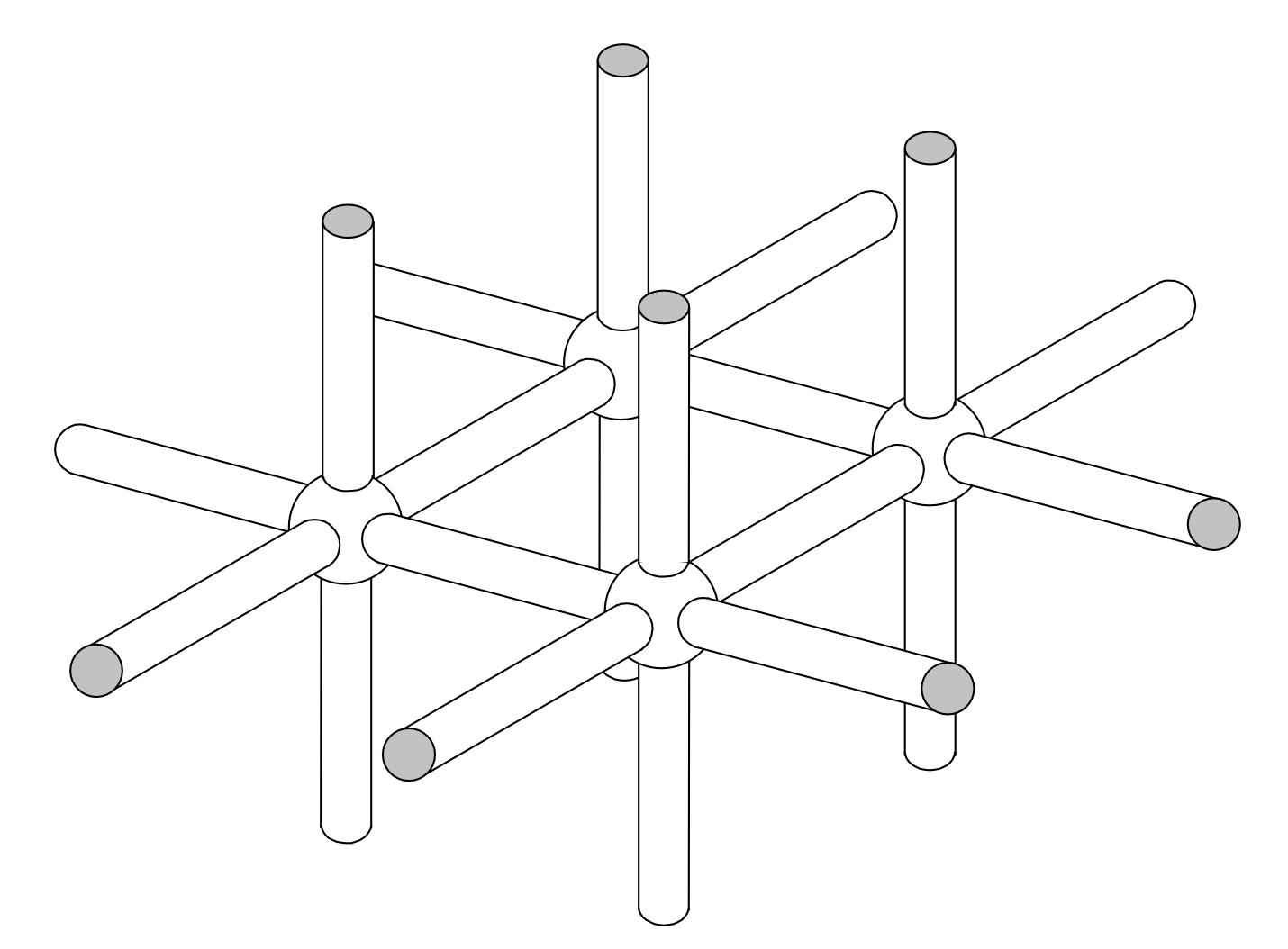
Figure 1. The two dimensional jungle-gym in $\mathbb{R}^{3}$. Picture taken from [16].

Start from the two dimensional jungle-gym $JG^{2}$ in $\mathbb{R}^{3}$ as in Figure 1. This is done by smoothly connecting the lattice $\mathbb{Z}^{3}\subset\mathbb{R}^{3}$ with necks. Let $g$ be the standard metric on $JG^{2}$ induced by the embedding in $\mathbb{R}^{3}$. Fix $o\in JG^{2}$ and let $r:=d(o,x)$. One can show that then $JG^{2}$ has the $L^{\infty}-{\rm Liouville}$ property. Moreover, there holds $\mu(B_{R}(o))\leq CR^{3}$, and the Green function grows at most as $G(o,x)\leq C/r$ for large $r$. Let $\rho:JG^{2}\to[0,+\infty)$ be a smooth positive function with $\rho=1$ in $[0,1]$ and $\rho(r)\sim\frac{1}{r\log(r)}$ for large $r$, and consider the conformal metric $\widehat{g}:=\rho^{2}(r)g$ on $JG^{2}$. We claim that $N:=(JG^{2},\widehat{g})$ has the desired properties. Since

$$\int_{1}^{\infty}\rho(r)dr=\infty\,,$$

then $N$ is geodesically complete and hence complete. Moreover, as the Laplacian is conformally invariant in dimension two, $JG^{2}$ with its standard metric and $N$ have the same harmonic functions, and thus $N$ also has the $L^{\infty}-{\rm Liouville}$ property and satisfies $(i)$. Denote by $\widehat{G}$ the Green’s function of $N$. Then, by the choice of $\rho$, for $R$ big

$$\int_{N\setminus B_{R}(o)}\widehat{G}(o,x)\,d\widehat{\mu}(x)=\int_{JG^{2}\setminus B_{R}(o)}G(o,x)\rho^{2}(r)\,d\mu(x)<+\infty\,,$$

and by [16, Corollary 6.7] this implies $(ii)$. Consequently, note that also

$$\int_{0}^{\infty}\mathcal{N}(p,t)\,dt =\int_{0}^{\infty}\int_{N}H_{N}(x,p,t)\,d\widehat{\mu}(x)dt=\int_{N}\left(\int_{0}^{\infty}H_{N}(x,p,t)\,dt\right)d\widehat{\mu}(x)$$

$$=\int_{N}\widehat{G}(o,x)\,d\widehat{\mu}(x)=\int_{N\setminus B_{R}(o)}\widehat{G}(o,x)\,d\widehat{\mu}(x)+\int_{B_{R}(o)}\widehat{G}(o,x)\,d\widehat{\mu}(x)<+\infty\,,$$

and since the function $\mathcal{N}(p,\cdot)$ is also nonincreasing this implies that $N$ also satisfies $(iii)$.

Now, the proof of our main theorem in the infinite volume case is just a simple application of all the result that we have derived above.

Proof of Theorem 1.6.

Write

$$\frac{1}{2}P_{s}(E,\Omega) =\mathcal{J}_{s}(E\cap\Omega,E^{c}\cap\Omega)+\mathcal{J}_{s}(E\cap\Omega,E^{c}\cap\Omega^{c})+\mathcal{J}_{s}(E\cap\Omega^{c},E^{c}\cap\Omega)$$

$$=\frac{1}{2}P_{s}(E\cap\Omega)-\mathcal{J}_{s}(E\cap\Omega,E\cap\Omega^{c})+\mathcal{J}_{s}(E^{c}\cap\Omega,E\cap\Omega^{c})\,.$$

By Corollary 5.4 and by Corollary 5.3, applied with $F=E\cap\Omega$ and $F=E^{c}\cap\Omega$, taking the limit as $s\to 0^{+}$ we get

$$\lim_{s\to 0^{+}}\frac{1}{2}P_{s}(E,\Omega) =\mu(E\cap\Omega)-\theta_{E}\mu(E\cap\Omega)+\theta_{E}\mu(E^{c}\cap\Omega)$$

$$=(1-\theta_{E})\mu(E\cap\Omega)+\theta_{E}\mu(E^{c}\cap\Omega)\,,$$

and this shows $(i)$.

To prove $(ii)$ and $(iii)$ we follow closely the proof of in [10, Theorem 2.7], which deals with the analogous property in the case of the Euclidean space $\mathbb{R}^{n}$. We just sketch the argument, since in the reference [10] the proof is carried on in full details and in our case it is analogous. Let us denote

$$\Theta_{s}(E):=\int_{E\setminus B_{R}(p)}\mathcal{K}_{s}(x,p)d\mu(x)\,,$$ (28)

and fix $R\gg 1$ such that $\Omega\subset B_{R}(p)$. Note that

$$\int_{\Omega\setminus E}\int_{E\setminus B_{R}(p)}\mathcal{K}_{s}(x,y)\,d\mu(x)d\mu(y)-\int_{\Omega\cap E}\int_{E\setminus B_{R}(p)}\mathcal{K}_{s}(x,y)\,d\mu(x)d\mu(y)$$

$$=\frac{1}{2}P_{s}(E,\Omega)-\frac{1}{2}P_{s}(E\cap\Omega,\Omega)-\mathcal{J}_{s}(\Omega\setminus E,(E\setminus\Omega)\cap B_{R}(p))+\mathcal{J}_{s}(\Omega\cap E,(E\setminus\Omega)\cap B_{R}(p))\,.$$

Now, arguing exactly as in the proof of Lemma 5.1 we have that for every bounded $F\subset M$ there holds

$$\lim_{s\to 0^{+}}\left|\mu(F)\Theta_{s}(E)-\int_{F}\int_{E\setminus B_{R}(p)}\mathcal{K}_{s}(x,y)\,d\mu(x)d\mu(y)\right|=0\,.$$

But also by Lemma 5.2 we have both

$$\lim_{s\to 0^{+}}\mathcal{J}_{s}(\Omega\setminus E,(E\setminus\Omega)\cap B_{R}(p))=0\,,$$

and

$$\lim_{s\to 0^{+}}\mathcal{J}_{s}(\Omega\cap E,(E\setminus\Omega)\cap B_{R}(p))=0\,.$$

Hence, taking the limit as $s\to 0^{+}$ above gives

$$\lim_{s\to 0^{+}}\Theta_{s}(E)\big{(}\mu(\Omega\setminus E)-\mu(\Omega\cap E)\big{)}=\lim_{s\to 0^{+}}\frac{1}{2}\big{(}P_{s}(E,\Omega)-P_{s}(E\cap\Omega,\Omega)\big{)}\,.$$

But since $E\cap\Omega\subset\Omega$ is bounded, by Corollary 5.4 we have

$$\lim_{s\to 0^{+}}\frac{1}{2}P_{s}(E\cap\Omega,\Omega)=\lim_{s\to 0^{+}}\frac{1}{2}P_{s}(E\cap\Omega)=\mu(E\cap\Omega)\,,$$

thus

$$\lim_{s\to 0^{+}}\Theta_{s}(E)\big{(}\mu(\Omega\setminus E)-\mu(\Omega\cap E)\big{)}=\lim_{s\to 0^{+}}\frac{1}{2}P_{s}(E,\Omega)-\mu(E\cap\Omega)\,.$$

From here, the conclusion of the theorem easily follows. Indeed, if $\mu(\Omega\setminus E)=\mu(\Omega\cap E)$ then the limit $\lim_{s\to 0^{+}}\frac{1}{2}P_{s}(E,\Omega)$ always exists and is equal to $\mu(E\cap\Omega)$. On the other hand, if the limit $\lim_{s\to 0^{+}}\frac{1}{2}P_{s}(E,\Omega)$ exists then from above the limit in $\theta_{E}$ also exists and there holds

$$\theta_{E}=\frac{\lim_{s\to 0^{+}}\frac{1}{2}P_{s}(E,\Omega)-\mu(E\cap\Omega)}{\mu(\Omega\setminus E)-\mu(E\cap\Omega)}\,,$$

and this concludes the proof. ∎

6. Extension to RCD spaces

In this section we briefly explain how our results extend to the case of ${\rm RCD}(K,N)$ spaces, which are a generalization of Riemannian manifolds with upper bound on the dimension $N$ and Ricci curvature bounded from below by the real number $K$ (and they include weighted manifolds). While assuming the reader familiar with the theory of ${\rm RCD}$ spaces we have to mention at least some references: the introduction of a synthetic lower bound on the Ricci curvature (${\rm CD}$ condition) has been done in the work of Lott and Villani [24] and in the works of Sturm [27], [28]. In a subsequent work Ambrosio, Gigli and Savarè introduced the ${\rm RCD}$ condition (see [1]) to rule out Finsler structures and enforce some Riemannian-like structure at small scales of the space (infinitesimal hilbertianity, see also [12]).

We stress that we won’t reprove every result of the smooth case but only the ones presenting major changes which are needed to perform the asymptotic analysis. First of all, on any ${\rm RCD}(K,N)$ space with $K\in\mathbb{R}$ and $N\in\mathbb{N}\cup\{\infty\}$ it is possible to define a heat kernel and to do so we shall exploit the theory of gradient flows. We call the heat flow $(e^{t\Delta})_{t>0}$ the gradient flow (in the sense of Komura-Brezis theory) of the Cheeger energy which displays the following properties: for an $L^{2}$ function $f$ the curve $t\in(0,\infty)\to e^{t\Delta}f\in L^{2}$ is locally absolutely continuous, it is such that $e^{t\Delta}f\in{\rm D}(\Delta)$, $\lim_{t\to 0}e^{t\Delta}f=f$ in $L^{2}$ and moreover satisfies the heat equation

$$\frac{de^{t\Delta}}{dt}=\Delta e^{t\Delta}f\quad\forall t>0.$$

We will now collect some other properties of the heat flow holding on infinitesimally hilbertian metric measure spaces which we will exploit (see [13] for a reference):

Proposition 6.1.

Let $(X,d,\mu)$ be an infinitesimally hilbertian metric measure space, then we have

• (Weak maximum principle): Given any $f\in L^{2}(\mu)$ such that $f\leq C$ $\mu$-almost everywhere we have

  $$e^{t\Delta}f\leq C\quad\mu-{\rm a.e.}$$

• ($e^{t\Delta}$ is self-adjoint): For all $f,g\in L^{2}(\mu)$ we have

  $$\int_{X}e^{t\Delta}fgd\mu=\int_{X}e^{t\Delta}gfd\mu\quad\forall t>0.$$

• ($\Delta$ and $e^{t\Delta}$ commute): For all $f\in{\rm D}(\Delta)$ we have

  $$\Delta e^{t\Delta}f=e^{t\Delta}\Delta f\quad\mu-{\rm a.e.},\;\forall t>0.$$

Moreover if $(X,d,\mu)$ is an ${\rm RCD}(K,\infty)$ space we have the following additional properties:

• (Bakry-Émery estimate): For all $f\in W^{1,2}(X)$ and $t>0$ we have

  $$|\nabla e^{t\Delta}f|^{2}\leq e^{-2Kt}e^{t\Delta}\bigl{(}|\nabla f|^{2}\bigr{)}\quad\mu-{\rm a.e.}$$ (29)

• ($L^{\infty}-{\rm Lip}$ regularization): For all $f\in L^{\infty}(\mu)$ and $t>0$ we have

  $$\|\nabla e^{t\Delta}f\|_{L^{\infty}(\mu)}\leq\frac{e^{-2Kt}}{\sqrt{t}}\|f\|_{L^{\infty}(\mu)}.$$ (30)

It is then possible to define the heat flow for all probability measures with finite second moment as the $EVI_{K}$ (again, we assume the reader to be familiar with the terminology) gradient flow of the entropy functional. More precisely for every $\mu\in\mathcal{P}_{2}(X)$, $e^{t\Delta}\mu$ (with a little abuse of notation here) is the unique measure such that

$$\int_{X}\varphi de^{t\Delta}\mu=\int_{X}e^{t\Delta}\varphi d\mu\quad\forall\varphi\in{\rm Lip}_{bs}(X),$$

where ${\rm Lip}_{bs}(X)$ is the set of Lipschitz functions with bounded support and $e^{t\Delta}\varphi$ is the Lipschitz continuous representative of its equivalence class (which is well-posed thanks to the $L^{\infty}-{\rm Lip}$ regularization property).

On ${\rm RCD}(K,\infty)$ it is possible to define the heat kernel $H_{X}(x,\cdot,t):=\frac{de^{t\Delta}\delta_{x}}{d\mu}$ and we have the following (see [21] for a reference):

Proposition 6.2.

Let $(X,d,\mu)$ be an ${\rm RCD}(K,N)$ space with $N\in\mathbb{N}$, then for all $\epsilon>0$, for some $C_{1},C_{2},C_{3},C_{4}$ nonnegative constants (possibly depending on $\epsilon$ and $N$) we have

$$\frac{1}{C_{1}\mu(B_{\sqrt{t}}(y))}\exp{\biggl{(}-\frac{d^{2}(x,y)}{(4-\epsilon)t}-C_{2}t\biggr{)}}\leq H_{X}(x,y,t)\leq\frac{C_{1}}{\mu(B_{\sqrt{t}}(y))}\exp{\biggl{(}-\frac{d^{2}(x,y)}{(4+\epsilon)t}+C_{2}t\biggr{)}}$$ (31)

for all $x,y\in X$, $t>0$ and

$$|\nabla H_{X}(x,\cdot,t)|(y)\leq\frac{C_{3}}{\sqrt{t}\mu(B_{\sqrt{t}}(y))}\exp{\biggl{(}\frac{-d^{2}(x,y)}{(4+\epsilon)t}-C_{4}t\biggr{)}}$$ (32)

$\mu\times\mu$-a.e. $(x,y)\in X\times X$, for all $t>0$.

Moreover, if $K=0$ then estimate (31) holds with $C_{2}=C_{4}=0$.

On any ${\rm RCD}(K,\infty)$ space we have

$$\int_{X}H_{X}(x,y,t)d\mu(x)=1$$

for all $y\in X$, $t>0$. That is, $X$ is stochastically complete.

In the setting of ${\rm RCD}(K,N)$ (actually infinitesimal hilbertianity is not required) we also have Bishop-Gromov’s comparison theorem, holding both for the perimeter measure and the volume measure (see [28]). Finally it is possible to prove that the following version of the Harnack inequality holds (see [22] for the proof)

Proposition 6.3 (Harnack inequality).

Let $(X,d,\mu)$ be an ${\rm RCD}(K,\infty)$ space, $p\in(1,\infty)$ and $f\in L^{1}(\mu)\cap L^{\infty}(\mu)$, then

$$|(e^{t\Delta}f)(x)|^{p}\leq(e^{t\Delta}|f|^{p})(y)\exp\biggl{(}\frac{pKd^{2}(x,y)}{2(p-1)(e^{2Kt}-1)}\biggr{)}$$

for all $x,y\in X\times X$ and $t>0$.

From the previous Harnack inequality it is possible to prove the following Gaussian bound (see [29, Theorem 4.1]) for ${\rm RCD}(K,\infty)$ spaces (compare with (31) above for ${\rm RCD}(K,N)$ spaces).

Proposition 6.4.

Let $(X,d,\mu)$ be an ${\rm RCD}(K,\infty)$ space, then there exists $C_{K}>0$ and for all $\varepsilon>0$ there exists $C_{\varepsilon}>0$ such that

$$H_{X}(x,y,t)\leq\frac{1}{\sqrt{\mu(B_{\sqrt{t}}(x))}\sqrt{\mu(B_{\sqrt{t}}(y))}}\exp\biggl{(}C_{\varepsilon}(1+C_{K})t-\frac{d^{2}(x,y)}{(4+\varepsilon)t}\biggr{)}.$$ (33)

If $K\geq 0$ one can take $C_{K}=0$.

The second ingredient we need is a generalization to ${\rm RCD}(K,\infty)$ spaces of the $L^{2}-{\rm Liouville}$ property of Yau (our Theorem 2.3).

Proposition 6.5.

Let $(X,d,\mu)$ be an ${\rm RCD}(K,\infty)$ space. Then, any $L^{2}(\mu)$ harmonic function is constant.

Proof.

Denote $w(t,x):=e^{t\Delta}u(x)$. Assume $u\in L^{2}(\mu)$ is harmonic, then by applying the heat flow to $\Delta u=0$ and using item $(iii)$ of Proposition 6.1 we have

$$\Delta w=0.$$

By gradient flow theory we have

$$\int_{X}|\nabla w|^{2}d\mu\leq\frac{1}{2t}\int_{X}|u|^{2}d\mu,$$

whence

$$0=-\int_{X}w\Delta w\,d\mu=\int_{X}|\nabla w|^{2}d\mu.$$

This means $|\nabla w|=0$ $\mu$-a.e. and by the Sobolev to Lipschitz property this implies that $w$ is constant, therefore there exists $C=C(t)$ such that $w(t,\cdot)=C(t)$. Now if $\mu(X)<\infty$ by using the stochastical completeness we can infer ($u\in L^{2}(\mu)$ implies $u\in L^{1}(\mu)$)

$$\int_{X}w\,d\mu=\int_{X}u\,d\mu=\mu(X)C(t),$$

hence $C$ does not actually depend on $t$ and by taking the limit as $t\to 0^{+}$ we infer that $u$ is constant. If $\mu(X)=\infty$ then for every $t$ we have $w=0$ because the only constant in $L^{2}(\mu)$ is zero and we conclude. ∎

Remark 6.6.

The previus proposition actually does not require a curvature condition: working in a space in which having zero weak upper gradient implies being constant is enough.

We then have the following result, which is a non-smooth analogue of Proposition 2.6.

Proposition 6.7.

Let $(X,d,\mu)$ be an ${\rm RCD}(K,\infty)$ space, then we have the following dicotomy:

• If $\mu(X)<+\infty$ then

  $$H_{X}(t,x,y)\to\frac{1}{\mu(X)}\quad{\rm as}\;t\to\infty\;\;\forall x,y\in X.$$

• If $\mu(X)=+\infty$ we have

  $$H_{X}(\cdot,\cdot,t)\to 0\quad{\rm as}\;t\to\infty$$ (34)

  locally uniformly and $H_{X}(p,\cdot,t)\to 0$ uniformly as $t\to\infty$ for every $p\in M$.

Proof.

For the proof of $(i)$ everything follows verbatim from the proof of Proposition 2.6. For what concerns the second point we shall exploit the Harnack inequality of Proposition 6.3. We repeat the first part of the proof for the sake of exposition: first let $f=H_{X}(p,\cdot,\varepsilon)$, then $\max\{\|e^{t\Delta}f\|_{L^{1}},\|e^{t\Delta}f\|_{L^{\infty}}\}\leq C$ due to the properties of the heat flow. Moreover by the semigroup property of it is easy to see that weak convergence in $L^{2}(\mu)$ of $e^{t\Delta}f$ is equivalent to strong convergence and we again have the inequality

$$|(e^{t\Delta}f,g)|\leq|(e^{t\Delta}f,f)\|(e^{t\Delta}g.g)|\leq\|g\|^{2}_{L^{2}(\mu)}|(e^{t\Delta}f,f)|$$

for all $t\in(0,\infty)$ and for all $f,g\in L^{2}(\mu)$. Now again using the spectral measure representation and Proposition 6.5 we infer the desired $L^{2}$ convergence. This convergence can be upgraded to be locally uniform by the Harnack inequality (Proposition 6.3) with $p=2$ and by the fact that $|f|^{2}\leq\|f\|_{L^{\infty}}|f|$, together with the maximum principle to get

$$|e^{t\Delta}f(x)|^{2}\leq\|f\|_{L^{\infty}}e^{t\Delta}(|f|)(y)\exp\biggl{(}\frac{2KR^{2}}{2(e^{2Kt}-1)}\biggr{)}$$

for every $y\in B_{R}(x)$. Integrating over the latter set in $d\mu(y)$ and taking the supremum allows to conclude. The global uniform convergence follows along the same lines of the smooth case. ∎

Remark 6.8.

As in the smooth case if $\mu(x)=\infty$ we have that for every $f\in L^{1}(\mu)$

$$\lim_{t\to\infty}e^{t\Delta}f(x)=0$$

for every $x\in X$.

We refer to [3] for an introduction to $H^{s}$ spaces on very general ambient space, like ${\rm RCD}$ spaces and more. We have the analogue of Theorem 4.1.

Theorem 6.9.

Let $(X,d,\mu)$ be an ${\rm RCD}(K,\infty)$ space with $K\in\mathbb{R}$ and $\mu(X)<+\infty$. Let $u\in H^{s_{\circ}/2}(X)$ for some $s_{\circ}\in(0,1)$ with bounded support. Then

$$\lim_{s\to 0^{+}}\frac{1}{2}[u]_{H^{s/2}(X)}^{2}=\|u\|_{L^{2}(X)}^{2}-\frac{1}{\mu(M)}\biggl{(}\int_{X}ud\mu\biggr{)}^{2}.$$

Proof.

The proof is exactly the same as in the smooth case exploiting the $L^{2}-{\rm Liouville}$ property of Proposition 6.5. ∎

To prove the convergence result for the case of infinite volume we need a convergence result for the solution of the heat equation to the initial datum. We therefore recall the following (upper) Large Deviation Principle on proper ${\rm RCD}(K,\infty)$ spaces (see [14, Theorem 5.3])

Theorem 6.10.

Let $(X,d,\mu)$ be a proper ${\rm RCD}(K,\infty)$ space, then for every $x\in X$ and closed set $C\subseteq X$ we have, setting $\mu_{t}[x]=H_{X}(\cdot,x,t)\mu$,

$$\limsup_{t\to 0}t\log(\mu_{t}[x](C))\leq-\inf_{y\in C}\frac{d^{2}(x,y)}{4}.$$ (35)

Remark 6.11.

In (35) we can choose $C=X\setminus B_{r}(p)$ and obtain the following estimate for small times (depending on $r>0$ and $\varepsilon>0$)

$$|e^{t\Delta}(\chi_{X\setminus B_{r}(p)})(p)|\leq\exp\bigg{(}-\frac{r^{2}-\varepsilon}{4t}\bigg{)}$$ (36)

We are finally ready to prove the following proposition (analogue of Proposition 1.4)

Proposition 6.12.

Let $(X,d,\mu)$ be a proper ${\rm RCD}(K,\infty)$ space with $\mu(X)=+\infty$. Then for every $p\in X$

$$\theta_{M}(p)=\lim_{s\to 0}\int_{X\setminus B_{1}(p)}\mathcal{K}_{s}(x,p)d\mu(x)=1.$$

Proof.

As for the smooth case we first show that

$$\lim_{s\to 0^{+}}\frac{s}{2}\int_{X\setminus B_{1}(p)}\int_{0}^{1}H_{X}(x,p,t)\frac{dt}{t^{1+s/2}}d\mu(x)=0.$$

Indeed there exists $\delta>0$ such that for all $t\leq\delta$ (36) holds, so that the previous integral can be estimated with the following

$$\frac{s}{2}\int_{0}^{\delta}e^{-r^{2}/5t}\frac{dt}{t^{1+s/2}}+\frac{s}{2}\int_{X\setminus B_{1}(p)}\int_{\delta}^{1}H_{X}(x,p,t)\frac{dt}{t^{1+s/2}}.$$

The first term clearly goes to zero as $s\to 0^{+}$ and to handle the second we use Fubini to deduce that (here stochastical completeness is not necessary but ${\rm RCD}(K,\infty)$ spaces enjoy this property so we write the equality sign)

$$\frac{s}{2}\int_{X\setminus B_{1}(p)}\int_{\delta}^{1}H_{X}(x,p,t)\frac{dt}{t^{1+s/2}}=\frac{s}{2}\int_{\delta}^{1}\frac{dt}{t^{1+s/2}}-\frac{s}{2}\int_{B_{1}(p)}\int_{\delta}^{1}H_{X}(x,p,t)\frac{dt}{t^{1+s/2}}d\mu(x).$$

Again the first term trivially goes to zero while for the second we apply (33) and exploit properness of the space to infer that $H_{X}(\cdot,\cdot,\cdot)$ is equibounded in $B_{1}(p)\times[\delta,1]$ so that

$$\limsup_{s\to 0}\biggl{|}\frac{s}{2}\int_{B_{1}(p)}\int_{\delta}^{1}H_{X}(x,p,t)\frac{dt}{t^{1+s/2}}d\mu(x)\biggr{|}\leq\limsup_{s\to 0^{+}}C\frac{s}{2}\int_{\delta}^{1}\frac{dt}{t^{1+s/2}}=0\,.$$

We now claim that

$$\lim_{s\to 0^{+}}\frac{s}{2}\int_{B_{1}(p)}\int_{1}^{\infty}H_{X}(x,p,t)\frac{dt}{t^{1+s/2}}d\mu(x)=0.$$

Indeed, thanks to the local uniform convergence proved in (34) and reasoning as in the previous step the latter result easily follows.

Finally we can perform the same steps and write

$$\theta_{M}(p)=\lim_{s\to 0}\frac{s}{2}\int_{X}\int_{1}^{\infty}H_{X}(x,y,t)\frac{dt}{t^{1+s/2}}d\mu(x),$$

which equals $1$ by using stochastical completeness. ∎

In the following proposition we study the behaviour of the singular kernel $\mathcal{K}_{s}(x,y)$.

Proposition 6.13.

Let $(X,d,\mu)$ be an ${\rm RCD}(K,N)$ space with $\mu(X)=+\infty$. Then, for every $x\in X$ which is a regular point we have

$$\frac{Cs}{r^{n+s}}\leq\mathcal{K}_{s}(x,y)\leq\frac{Cs}{r^{n+s}}+o_{s}(1)+\sup_{t\geq 1/s}H_{M}(x,y,t),$$ (37)

for every $y\in X$, where $r=d(x,y)$. In particular $\mathcal{K}_{s}(x,\cdot)\to 0$ as $s\to 0^{+}$ locally uniformly away from $x$.

Proof.

Let us define

$$\mathcal{K}_{s}(x,y) =\frac{s}{2}\int_{0}^{1}H_{X}(x,y,t)\frac{dt}{t^{1+s/2}}+\frac{s}{2}\int_{1}^{1/s}H_{X}(x,y,t)\frac{dt}{t^{1+s/2}}+\frac{s}{2}\int_{1/s}^{\infty}H_{X}(x,y,t)\frac{dt}{t^{1+s/2}}$$

$$=:I_{1}+I_{2}+I_{3}.$$

By the Gaussian estimates (31) amd using the fact that $x$ is a regular point we have

$$I_{1}\leq Cs\int_{0}^{1}e^{-r^{2}/5t}\frac{dt}{t^{1+s/2+n/2}}\leq\frac{Cs}{r^{n+s}}.$$

Moreover, since $\mu(X)=+\infty$ by (34) the heat kernel converges locally uniformly to zero, and we also get

$$I_{2}\leq Cs\int_{1}^{1/s}\frac{dt}{t^{1+s/2}}=C(1-s^{s/2})=o_{s}(1),$$

for some constant $C$ which is bounded in a neighborhood of $x$. Finally we have

$$I_{3}\leq\frac{s}{2}\sup_{t\geq 1/s}H_{M}(x,y,t)\int_{1/s}^{\infty}\frac{dt}{t^{1+s/2}},$$

thus proving the upper bound in (6.13). For the lower bound it is enough to neglect $I_{2}$ and $I_{3}$ and apply the Gaussian estimate from below to $I_{1}$.

Finally, the local uniform convergence $\mathcal{K}_{s}(x,\cdot)\to 0$ is apparent due to the local uniform convergence (34) of the heat kernel to zero and the other quantities involved. ∎

With the next proposition we show that the heat density of a set, whenever it exists, is independent of the radius and also on the point if the $L^{\infty}-{\rm Liouville}$ property holds, analogously to the case of manifolds.

Proposition 6.14.

Let $(X,d,\mu)$ be an ${\rm RCD}(K,\infty)$ space with $\mu(X)=+\infty$ and let $E\subset M$ such that $\theta_{E}$ exists, then

$$\theta_{E}(p)=\lim_{s\to 0^{+}}\int_{X\setminus B_{r}(p)}\mathcal{K}_{s}(p,x)d\mu(x)$$

for all $r>0$. Moreover, if the $L^{\infty}-{\rm Liouville}$ property holds then the latter quantity is independent also of the point $p$.

Proof.

We first show the independence on the radius, therefore we fix any two $0<r<R$ and we show that

$$\limsup_{s\to 0^{+}}\frac{s}{2}\int_{\overline{B_{R}(p)}\setminus B_{r}(p)}\int_{0}^{\infty}H_{X}(x,p,t)\frac{dt}{t^{1+s/2}}d\mu(x)=0.$$

We split the integral over the time in three pieces: one from $0$ to $\varepsilon$, one from $\varepsilon$ to $T$ and the last one from $T$ to $\infty$. The first piece goes to zero since $\overline{B_{R}(p)}\setminus B_{r}(p)$ is a closed set and we can apply (36), the second piece goes to zero for every $T\gg 1$ thanks to the properness of the space, the Gaussian upper bound (33) and easy calculations, while the last piece is such that, for all $T\geq T_{0}(\varepsilon)$

$$\limsup_{s\to 0}\frac{s}{2}\int_{T}^{\infty}H_{X}(x,p,t)\frac{dt}{t^{1+s/2}}d\mu(x)\leq\varepsilon.$$

Since this holds for every $\varepsilon$ we get the convergence to zero.

For what concerns the independence on the point we first take $r$ so big that $q\in B_{r/10}(p)$ and wlog we assume $E$ to be closed. We have

$$\limsup_{s\to 0^{+}}\biggl{|}\int_{E\setminus B_{r}(p)}\mathcal{K}_{s}(x,p) d\mu(x)-\int_{E\setminus B_{2r}(q)}\mathcal{K}_{s}(x,q)d\mu(x)\biggr{|}$$

$$\leq\limsup_{s\to 0^{+}}\biggl{|}\int_{E\setminus B_{r}(p)}\mathcal{K}_{s}(x,q)d\mu(x)-\int_{E\setminus B_{2r}(q)}\mathcal{K}_{s}(x,q)d\mu(x)\biggr{|}$$

$$+\limsup_{s\to 0^{+}}\biggl{|}\int_{E\setminus B_{r}(p)}\mathcal{K}_{s}(x,p)-\mathcal{K}_{s}(x,q)d\mu(x)\biggr{|}=:I_{1}+I_{2}.$$

The first integral is zero since

$$I_{1}\leq\limsup_{s\to 0^{+}}\int_{B_{2r}(q)\setminus B_{r}(p)}\mathcal{K}_{s}(x,q)d\mu(x)=\theta_{B_{2r}(q)}(q)=0\,,$$

where we have used the independence on the radius. While for $I_{2}$ we shall exploit the $L^{\infty}-{\rm Liouville}$ property. We can, as usual, expand the singular kernel and split the integral in time into three pieces, one going from $0$ to $1$, another from $1$ to $T\gg 1$ and lastly from $T$ to $\infty$. The first two are handled thanks to the exponential convergence (36) and the boundedness of the heat kernel, while for the last one we have

$$\limsup_{s\to 0^{+}}\bigg{|}\int_{T}^{\infty}e^{t\Delta}(\chi_{E\setminus B_{r}(p)})(p)-e^{t\Delta}(\chi_{E\setminus B_{r}(p)})(q)\frac{dt}{t^{1+s/2}}\bigg{|}=0$$

thanks to the $L^{\infty}-{\rm Liouville}$ property. Indeed $e^{t\Delta}(\chi_{E\setminus B_{r}(p)})$ converges up to subsequences to a constant harmonic function, hence its (of the limit function) value at the points $p$ and $q$ is the same so that, being this true for any subsequence, $e^{t\Delta}(\chi_{E\setminus B_{r}(p)})(p)-(\chi_{E\setminus B_{r}(p)})(q)\to 0$ as $t\to\infty$. ∎

Finally we have the analogue of Theorem 3.5.

Theorem 6.15.

Let $(X,d,\mu)$ be a proper ${\rm RCD}(K,N)$ space with $\mu(X)=+\infty$ and $N<+\infty$, and let $s_{\circ}\in(0,1)$. Then for every $u\in H^{s_{\circ}/2}(X)\cap L^{\infty}(X)$ with bounded support there holds

$$\lim_{s\to 0^{+}}\frac{1}{2}[u]_{H^{s/2}(X)}^{2}=\|u\|_{L^{2}(X)}^{2}.$$

Proof.

The proof is similar to the smooth case, we just need to handle with a bit more care the computations. We advise the reader to first see the proof in the smooth case of Theorem 3.5.

By Proposition 7.5 (which also holds for ${\rm RCD}$ spaces, see Remark 7.6) for $\mu$-a.e. $x\in X$ the integral in $(-\Delta)^{s/2}_{\rm Si}u$ is absolutely convergent. Fix $x\in X$ is this full-measure set and $R>0$ such that $\operatorname{supp}(u)\subseteq B_{R}(x)$. Now we prove that, as $s\to 0^{+}$, $(-\Delta)^{s/2}_{\rm Si}u\to u$ $\mu$-a.e. with the same strategy of the smooth case. Take also $x\in X$ to be a regular point, we have

$$(-\Delta)^{s/2}_{\rm Si}u(x)=\int_{B_{R}(x)}(u(x)-u(y))\mathcal{K}_{s}(x,y)d\mu(y)+u(x)\int_{X\setminus B_{R}(x)}\mathcal{K}_{s}(x,y)d\mu(y)$$

and we are left to prove that the first term goes to zero as $s\to 0^{+}$, as the second one in the limit is precisely $u(x)$. Now fix $\rho\ll 1$ and let us split the first integral as follows

$$\bigg{|}\int_{B_{R}(x)}(u(x)-u(y))\mathcal{K}_{s}(x,y)\,d\mu(y)\bigg{|} =\int_{B_{\rho}(x)}|u(x)-u(y)|\mathcal{K}_{s}(x,y)\,d\mu(y)$$

$$\hskip 7.0pt\hskip 7.0pt+\int_{B_{R}(x)\setminus B_{\rho}(x)}|u(x)-u(y)|\mathcal{K}_{s}(x,y)\,d\mu(y).$$

For the first integral we can apply Proposition 6.13 to obtain

$$\int_{B_{\rho}(x)}|u(x)-u(y)|\mathcal{K}_{s}(x,y)\,d\mu(y)\leq Cs\int_{B_{\rho}(x)}\frac{|u(x)-u(y)|}{d(x,y)^{n+s}}d\mu(y)+o_{s}(1).$$ (38)

Applying Hölder inequality as in the smooth case (take $s$ small so that $2s<s_{0}$) we now get

$$\int_{B_{\rho}(x)}\frac{|u(x)-u(y)|}{d(x,y)^{n+s}}\,d\mu(y)\leq\left(\int_{B_{\rho}(x)}\frac{(u(x)-u(y))^{2}}{d(x,y)^{n+s_{\circ}}}\,dy\right)^{1/2}\left(\int_{B_{\rho}(x)}\frac{1}{d(x,y)^{n+2s-s_{\circ}}dy}\right)^{1/2}$$

and conclude in the same way that taking the limit as $s\to 0^{+}$ in (38) gives zero. For the second term we just use the fact that $\mathcal{K}_{s}(x,\cdot)$ goes to zero locally uniformly away from $x$ together with dominated convergence. Therefore we have proved that $(-\Delta)^{s/2}_{\rm Si}u\to u$ $\mu$-a.e. as $s\to 0^{+}$. Now to establish the convergence of the seminorms we exploit Corollary 7.9, which holds also in this non-smooth setting with the same proof. To conclude we just need to prove that $(-\Delta)^{s/2}_{\rm Si}u\rightharpoonup u$ weakly in $L^{2}(\mu)$: this is however apparent because of the equiboundedness of $\|(-\Delta)^{s/2}_{\rm Si}u\|_{L^{2}(\mu)}$ given by the estimate (40). ∎

Thanks to the previous results we would be in the position of stating and proving (which we won’t do, since the proofs are exactly the same as in the smooth case) the theorems regarding the asymptotics of the fractional perimeter Theorem 1.8 and Theorem 1.6, also in this non-smooth setting.

7. Appendix

7.1. Heat kernel estimates and $H^{s}(M)$ spaces.

Here $(M,g)$ denotes a complete, connected Riemannian manifold. First, we present a simple interpolation inequality for $H^{s/2}(M)$ spaces.

This inequality is known in the case of $M=\mathbb{R}^{n}$ or $M=\Omega\subset\mathbb{R}^{n}$ for fractional Sobolev spaces $W^{s,p}$, also when $p\neq 2$. Here we carry on a structural proof using few properties of the heat kernel, and this gives the interpolation inequality on general ambient spaces.

Lemma 7.1.

Let $u\in H^{\sigma}(M)$ for some $\sigma\in(0,1)$, and let $0<s<\sigma<1$. Then $u\in H^{s}(M)$ and the following inequality holds

$$[u]_{H^{s}(M)}\leq C\|u\|_{L^{2}(M)}^{1-s/\sigma}[u]_{H^{\sigma}(M)}^{s/\sigma}.$$

for some absolute constant $C>0$.

Proof.

We have

$$|\Gamma(-s)|[u]_{H^{s}(M)}^{2} =\iint_{M\times M}(u(x)-u(y))^{2}\int_{0}^{\infty}H_{M}(x,y,t)\frac{dt}{t^{1+s}}d\mu(x)d\mu(y)$$

$$\leq\iint_{M\times M}(u(x)-u(y))^{2}\int_{0}^{\xi}H_{M}(x,y,t)\frac{dt}{t^{1+s}}d\mu(x)d\mu(y)$$

$$+\iint_{M\times M}(u(x)-u(y))^{2}\int_{\xi}^{\infty}H_{M}(x,y,t)\frac{dt}{t^{1+s}}d\mu(x)d\mu(y)$$

where $\xi\in(0,\infty)$ will be chosen at the end. Note that for all $t\in(0,\xi)$ we have $(\xi/t)^{1+s}\leq(\xi/t)^{1+\sigma}$ so that we can estimate from above the first integral of the previous inequality with

$$\xi^{\sigma-s}\iint_{M\times M}(u(x)-u(y))^{2}\int_{0}^{\xi}H_{M}(x,y,t)\frac{dt}{t^{1+\sigma}}d\mu(x)d\mu(y)\leq\xi^{\sigma-s}|\Gamma(-\sigma)|[u]^{2}_{H^{\sigma}(M)}.$$

The symmetry of the heat kernel and the fact that $\mathcal{M}(t,y)\leq 1$, for all $y\in M$, together imply that the second integral can be bounded by

$$\iint_{M\times M}(u(x)-u(y))^{2}\int_{\xi}^{\infty}H_{M}(x,y,t)\frac{dt}{t^{1+s}}d\mu(x)d\mu(y)\leq\frac{4}{s\xi^{s}}\|u\|^{2}_{L^{2}(M)}.$$

This two inequalities lead to

$$|\Gamma(-s)|[u]_{H^{s}(M)}^{2}\leq\xi^{\sigma-s}|\Gamma(-\sigma)|[u]^{2}_{H^{\sigma}(M)}+\frac{4}{s\xi^{s}}\|u\|^{2}_{L^{2}(M)}.$$

Optimizing the right-hand side in $\xi$ gives that the optimal value is

$$\xi=\biggl{(}\frac{4\|u\|_{L^{2}(M)}^{2}}{(\sigma-s)|\Gamma(-\sigma)|[u]^{2}_{H^{\sigma}(M)}}\biggr{)}^{1/\sigma}.$$

Putting everything together gives

$$|\Gamma(-s)|[u]^{2}_{H^{s}(M)}\leq\frac{C}{s}\|u\|_{L^{2}(M)}^{2(1-s/\sigma)}[u]_{H^{\sigma}(M)}^{2s/\sigma}\,,$$

and this implies

$$[u]_{H^{s}(M)}\leq C\|u\|_{L^{2}(M)}^{1-s/\sigma}[u]_{H^{\sigma}(M)}^{s/\sigma}\,,$$

as desired. ∎

Lemma 7.2 ([8]).

Let $(M^{n},g)$ be a complete $n$-dimensional Riemannian manifold and let $B_{R}(p)\subset M$. Then

$$e^{t\Delta}(\chi_{M\setminus B_{R}(p)})(p)=\int_{M\setminus B_{R}(p)}H_{M}(x,p,t)\,d\mu(x)\leq Ce^{-c/t}\,,$$

for some $C,c>0$ depending on $R$ and the geometry of $M$ in $B_{R}(p)$.

Proof.

This is essentially [8, Lemma 2.9]. Indeed, in [8, Lemma 2.9] the authors prove that if $(M,g)$ is a complete Riemannian manifold and $B_{r}(p)\subset M$ is a ball diffeomorphic to $\mathcal{B}_{r}(0)\subset T_{p}M$ with metric coefficients $g_{ij}$ (say, in normal coordinates) uniformly close to $\delta_{ij}$, then

$$\int_{M\setminus B_{r}(p)}H_{M}(x,p,t)\,d\mu(x)\leq Ce^{-c\,r^{2}/t}\,,$$

for some $C,c>0$ dimensional. Then, taking $r\ll 1$ very small and writing

$$\int_{M\setminus B_{R}(p)}H_{M}(x,p,t)\,d\mu(x)\leq\int_{M\setminus B_{r}(p)}H_{M}(x,p,t)\,d\mu(x)$$

allows to bound the desired integral. ∎

Now we present the proof of Lemma 3.4, that we needed to prove the asymptotics of the full $H^{s/2}(M)$ seminorm of Theorem 3.5.

Proof of Lemma 3.4.

Let $\varphi^{-1}:B_{1}(p)\to\mathbb{R}^{n}$ be the inverse of the exponential map at $p$. Take $\eta\in C^{\infty}_{c}(\mathcal{B}_{4/5}(0))$ with $\chi_{\mathcal{B}_{2/5}(0)}\leq\eta\leq\chi_{\mathcal{B}_{4/5}(0)}$ and let $g^{\prime}_{ij}:=g_{ij}\eta+(1-\eta)\delta_{ij}$. This is a metric on $\mathbb{R}^{n}$ with $g^{\prime}_{ij}=g_{ij}$ in $\mathcal{B}_{2/5}(0)$. Denote by $\mathcal{K}_{s},\mathcal{K}_{s}^{\prime}$ the singular kernels of $(M,g)$ and $M^{\prime}:=(\mathbb{R}^{n},g^{\prime})$ respectively. Let $\Lambda:=\sup_{x\in B_{1/5}(p)}H_{M}(x,x,1)$ and $\Lambda^{\prime}:=\sup_{x\in\mathcal{B}_{1/5}(0)}H_{M^{\prime}}(x,x,1)$. Then, by [8, Lemma 2.10] applied to the Riemannian manifolds $(M,g)$ and $(\mathbb{R}^{n},g^{\prime})$ we have, for $x,y\in\mathcal{B}_{1/5}(0)$

$$\big{|}\mathcal{K}_{s}(\varphi(x),\varphi(y)) -\mathcal{K}_{s}^{\prime}(x,y)\big{|}\leq\frac{s/2}{\Gamma(1-s/2)}\int_{0}^{\infty}\big{|}H_{M}(\varphi(x),\varphi(y),t)-H_{M^{\prime}}(x,y,t)\big{|}\frac{dt}{t^{1+s/2}}$$

$$\leq Cs(2-s)\int_{0}^{1}\big{|}H_{M}(\varphi(x),\varphi(y),t)-H_{M^{\prime}}(x,y,t)\big{|}\frac{dt}{t^{1+s/2}}$$

$$+Cs(2-s)\int_{1}^{1/s}\big{|}H_{M}(\varphi(x),\varphi(y),t)-H_{M^{\prime}}(x,y,t)\big{|}\frac{dt}{t^{1+s/2}}$$

$$+Cs(2-s)\int_{1/s}^{\infty}\big{|}H_{M}(\varphi(x),\varphi(y),t)-H_{M^{\prime}}(x,y,t)\big{|}\frac{dt}{t^{1+s/2}}$$

$$:=Cs(2-s)\big{[}I_{1}+I_{2}+I_{3}\big{]}\,.$$

By [8, Lemma 2.10] there holds

$$I_{1}=\int_{0}^{1}\big{|}H_{M}(\varphi(x),\varphi(y),t)-H_{M^{\prime}}(x,y,t)\big{|}\frac{dt}{t^{1+s/2}}\leq C\int_{0}^{1}e^{-c/t}\frac{dt}{t^{1+s/2}}\leq C\,,$$

for some dimensional $C=C(n)>0$. Regarding the second integral

$$I_{2}\leq\int_{1}^{1/s}(\Lambda+\Lambda^{\prime})\frac{dt}{t^{1+s/2}}=(\Lambda+\Lambda^{\prime})\frac{1-s^{s/2}}{s/2}\,,$$

and lastly

$$I_{3} =\int_{1/s}^{\infty}\big{|}H_{M}(\varphi(x),\varphi(y),t)-H_{M^{\prime}}(x,y,t)\big{|}\frac{dt}{t^{1+s/2}}$$

$$\leq s^{s/2}\int_{1}^{\infty}\bigg{[}H_{M}(\varphi(x),\varphi(y),\xi/s)+H_{M^{\prime}}(x,y,\xi/s)\bigg{]}\frac{d\xi}{\xi^{1+s/2}}=o_{s}(1)\to 0$$

as $s\to 0^{+}$, since both $M$ and $M^{\prime}$ have infinite volume and thus their heat kernel tends to zero as $t\to+\infty$ (see Lemma 2.6). Hence as $s\to 0^{+}$

$$\big{|}\mathcal{K}_{s}(\varphi(x),\varphi(y))-\mathcal{K}_{s}^{\prime}(x,y)\big{|}\leq Cs+C(\Lambda+\Lambda^{\prime})(1-s^{s/2})+o_{s}(1)=o_{s}(1)\,,$$

and note that this estimate is uniform in $x,y\in\mathcal{B}_{1/5}(0)$. This follows, for example, from the parabolic Harnack inequality since one can locally estimate the supremum of $H_{M}$ and $H_{M^{\prime}}$ with the $L^{1}$ norm at later times; see the end of the proof of Lemma 2.6. Then

$$\lim_{s\to 0^{+}}\sup_{x,y\in B_{1/8}(p)}\left|\mathcal{K}_{s}(x,y)-\mathcal{K}_{s}^{\prime}(x,y)\right|=0\,.$$

Lastly, by [8, Lemma 2.5] there exists dimensional constants $c,C>0$ such that

$$c\frac{\beta_{n,s}}{d(x,y)^{n+s}}\leq\mathcal{K}_{s}^{\prime}(x,y)\leq C\frac{\beta_{n,s}}{d(x,y)^{n+s}}\,,$$

and this concludes the proof. ∎

7.2. On the equivalence and well-posedness of different fractional Laplacians.

In this subsection we shall prove some results concerning the equivalence between different definitions of the fractional Laplacian, and the fractional Sobolev seminorms on (possibly weighted) Riemannian manifolds.

Next we want to show that the fractional laplacian defined with the heat semigroup $(-\Delta)^{s/2}_{\rm B}$ and the one defined via the singular integral $(-\Delta)^{s/2}_{\rm Si}$ coincide. Note that the two following propositions do not hold when $M$ is not stochastically complete. Indeed, using definition (14) gives $(-\Delta)^{s/2}_{\rm Si}(1)\equiv 0$, while if $M$ is not stochastically complete equation (12) gives $(-\Delta)^{s/2}_{\rm B}(1)\neq 0$.

Proposition 7.3.

Let $(M,g)$ be a complete, stochastically complete Riemannian manifold, and let $u\in C^{\infty}_{c}(M)$. Then:

• For $s<1$ the integral in $(-\Delta)^{s/2}_{\rm Si}u$ is absolutely convergent and the principal value is not needed.

• The singular integral $(-\Delta)^{s/2}_{\rm Si}u$ (defined in (14)) and the Bochner $(-\Delta)^{s/2}_{\rm B}u$ (defined in (12)) definition coincide.

Proof.

For what concerns the absolute convergence for $s\in(0,1)$, we have

$$\int_{M}(u(x)-u(y))\mathcal{K}_{s}(x,y)d\mu(y) =\int_{B_{r}(x)}(\dotsc)\,d\mu(y)+\int_{M\setminus B_{r}(x)}(\dotsc)\,d\mu(y)=:I_{1}+I_{2}.$$

For $r$ small, arguing exactly as in the proof of Theorem 3.5

$$I_{1}\leq C\int_{B_{r}(x)}\frac{1}{d(x,y)^{n+s-1}}d\mu(y)\leq C\int_{0}^{r}\frac{1}{\rho^{s}}d\rho<+\infty\,.$$

On the other hand, for the second integral

$$I_{2}\leq 2\|u\|_{L^{\infty}}\int_{M\setminus B_{r}(x)}\mathcal{K}_{s}(x,y)d\mu(y)\,,$$

and thanks to Lemma 7.2 and Fubini

$$\int_{M\setminus B_{r}(x)}\mathcal{K}_{s}(x,y)d\mu(y) =\int_{0}^{\infty}\frac{1}{t^{1+s/2}}\int_{M\setminus B_{r}(x)}H_{M}(x,y,t)d\mu(y)dt$$

$$\leq C\int_{0}^{1}e^{-c/t}\frac{dt}{t^{1+s/2}}+\int_{1}^{\infty}\frac{1}{t^{1+s/2}}dt<+\infty.$$

This concludes the proof of $(i)$.

Now, let us define

$$\mathfrak{J}(t):=\frac{e^{t\Delta}u(x)-u(x)}{t^{1+s/2}}=\frac{1}{t^{1+s/2}}\int_{M}H_{M}(x,y,t)(u(y)-u(x))d\mu(y),$$

where the second equality is due to the stochastical completeness. Note that $\mathfrak{J}\in L^{1}(0,+\infty)$ since $|e^{t\Delta}u(x)-u(x)|\leq Ct$, where the constant $C$ depends on $\|\Delta u\|_{L^{\infty}}$. We can now define

$$\mathfrak{J}_{k}(t):=\frac{1}{t^{1+s/2}}\int_{M\setminus B_{1/k}(x)}H_{M}(x,y,t)(u(y)-u(x))d\mu(y).$$

and observe that $\mathfrak{J}_{k}(t)\to\mathfrak{J}(t)$ for all $t\in(0,\infty)$. Now if $t\geq 1$ (estimating the mass of the heat kernel by $1$) we get $\mathfrak{J}_{k}(t)\leq 2\|u\|_{L^{\infty}}/t^{1+s/2}$, while by [8, Lemma 2.11] we have

$$\big{|}\mathfrak{J}(t)-\mathfrak{J}_{k}(t)\big{|} \leq\frac{1}{t^{1+s/2}}\int_{B_{1/k}(x)}H_{M}(x,y,t)|u(y)-u(x)|d\mu(y)$$

$$\leq\frac{C}{t^{1+s/2+n/2}}\int_{B_{1/k}(x)}e^{-d^{2}(x,y)/5t}d(x,y)d\mu(y)\,.$$

Applying Coarea formula and using the fact that ${\rm Per}(B_{r}(x))\leq Cr^{n-1}$ if $k$ is big we get

$$\big{|}\mathfrak{J}(t)-\mathfrak{J}_{k}(t)\big{|}\leq\frac{C}{t^{1+s/2+n/s}}\int_{0}^{1/k}e^{-r^{2}/5t}r^{n}dr=\frac{C}{t^{s/2}}\int_{0}^{1/(5tk^{2})}e^{-z}z^{n/2-1}dz\leq\frac{C}{t^{s/2}}.$$

Therefore if $t\geq 1$ we have $\mathfrak{J}_{k}(t)\leq C/t^{1+s/2}\in L^{1}(1,+\infty)$ while if $t\leq 1$ we have $\mathfrak{J}_{k}(t)\leq C/t^{s/2}+\mathfrak{J}(t)\in L^{1}(0,1)$. Hence by dominated convergence we can write

$$(-\Delta)^{s/2}_{\rm B}u(x)=\int_{0}^{\infty}\mathfrak{J}(t)\,dt=\lim_{k\to\infty}\int_{0}^{\infty}\int_{M\setminus B_{1/k}(x)}(u(y)-u(x))H_{M}(x,y,t)\frac{dt}{t^{1+s/2}}\,d\mu(y).$$

Now for any $k\in\mathbb{N}$ fixed, by Lemma (7.2) and the fact that $u$ is bounded, we get

$$\int_{0}^{\infty}\int_{M\setminus B_{1/k}(x)}|u(y)-u(x)|H_{M}(x,y,t)\frac{dt}{t^{1+s/2}}\leq 2\|u\|_{L^{\infty}}\int_{0}^{1}e^{-c/t}\frac{dt}{t^{1+s/2}}+2\|u\|_{L^{\infty}}\int_{1}^{\infty}\frac{dt}{t^{1+s/2}}<+\infty.$$

Therefore we can apply Fubini and infer

$$(-\Delta)^{s/2}_{\rm B}u(x) =\lim_{k\to\infty}\int_{M\setminus B_{1/k}(x)}\int_{0}^{\infty}(u(y)-u(x))H_{M}(x,y,t)\frac{dt}{t^{1+s/2}}\,d\mu(y)$$

$$={\rm P.V.}\int_{M}(u(y)-u(x))\mathcal{K}_{s}(x,y)d\mu(y).$$

∎

Remark 7.4.

One can note that the proof above of the absolute convergence of $(-\Delta)^{s/2}_{\rm Si}u$ for $s\in(0,1)$ actually shows that the integral is absolutely convergent if $u\in C^{\alpha}_{\rm loc}(M)\cap L^{\infty}(M)$ for some $\alpha>s$.

Regarding the following two results, we couldn’t find any proof in the case of an ambient Riemannian manifold $(M,g)$, even though they appear to be well-known in the community in the case $M=\mathbb{R}^{n}$ or a domain $M=\Omega\subset\mathbb{R}^{n}$. For example, a proof that ${\rm Dom}((-\Delta_{\Omega})^{s/2}_{\rm Spec})=H^{s}(\Omega)$ for the Dirichlet Laplacian on $\Omega\subset\mathbb{R}^{n}$ can be found in [4, Section 3.1.3], but it heavily uses the discreteness of the spectrum and interpolation theory.

Our results are not sharp, in particular, we believe that Proposition 7.5 and 7.7 hold also for $s=\sigma$ since this is the case for domains in $\mathbb{R}^{n}$. Here we focus on providing structural (and short) proofs that apply verbatim to the case of any weighted manifold, and we avoid using any local Euclidean-like structure of $M$.

Proposition 7.5.

Let $(M,g)$ be a stochastically complete Riemannian manifold, $\sigma\in(0,1)$ and $u\in H^{\sigma}(M)$ (as defined in Definition 1.9). Then, for every $s<\sigma$ the singular integral $(-\Delta)^{s/2}_{\rm Si}u$ (defined in (14)) and the Bochner $(-\Delta)^{s/2}_{\rm B}u$ (defined in (12)) definition coincide a.e. Moreover $(-\Delta)^{s/2}_{\rm B}u=(-\Delta)^{s/2}_{\rm Si}u\in L^{2}(M)$.

Proof.

Let $u\in H^{\sigma}(M)$ and $x\in M$. Since $M$ is stochastically complete, if we could exhange the order of integration we would have

$$(-\Delta)^{s/2}_{\rm B}u(x) =\frac{1}{\Gamma(-s/2)}\int_{0}^{\infty}(e^{t\Delta}u(x)-u(x))\frac{dt}{t^{1+s/2}}$$

$$=\frac{1}{\Gamma(-s/2)}\int_{0}^{\infty}\left(\int_{M}H_{M}(x,y,t)(u(y)-u(x))d\mu(y)\right)\frac{dt}{t^{1+s/2}}$$

$$=\int_{M}(u(y)-u(x))\mathcal{K}_{s}(x,y)d\mu(y)=(-\Delta)_{\rm Si}^{s/2}u(x)\,.$$

Now we shall justify the steps above, showing that the integral is absolutely convergent. Note that this will also justify the last equality, since we have defined $(-\Delta)_{\rm Si}^{s/2}$ with the Cauchy principal value. In particular, we show that

$$\int_{M}\left(\int_{M}|u(x)-u(y)|\mathcal{K}_{s}(x,y)d\mu(y)\right)^{2}d\mu(x)<+\infty\,.$$

This will prove at the same time that the integral above is absolutely convergent for a.e. $x\in M$ and that $(-\Delta)^{s/2}_{\rm Si}u\in L^{2}(M)$. Let us call

$$\mathfrak{I}(t):=\int_{M}|u(x)-u(y)|H_{M}(x,y,t)\,d\mu(y)\,,$$

and denote by $C$ a constant that depends at most on $\sigma$.

Note that, by Jensen’s inequality

$$\int_{0}^{\infty}\mathfrak{I}(t)^{2}\frac{dt}{t^{1+\sigma}} =\int_{0}^{\infty}\left(\int_{M}|u(x)-u(y)|H_{M}(x,y,t)\,d\mu(y)\right)^{2}\frac{dt}{t^{1+\sigma}}$$

$$\leq\int_{0}^{\infty}\int_{M}|u(x)-u(y)|^{2}H_{M}(x,y,t)\,d\mu(y)\frac{dt}{t^{1+\sigma}}$$

$$=C\int_{M}|u(x)-u(y)|^{2}\mathcal{K}_{2\sigma}(x,y)\,d\mu(y)\,.$$ (39)

Write

$$\int_{M}\bigg{(}\int_{M}|u(x)-u(y)| \mathcal{K}_{s}(x,y)d\mu(y)\bigg{)}^{2}d\mu(x)$$

$$=Cs^{2}\int_{M}\left(\int_{0}^{\infty}\mathfrak{I}(t)\frac{dt}{t^{1+s/2}}\right)^{2}d\mu$$

$$\leq Cs^{2}\int_{M}\left(\int_{0}^{1}\mathfrak{I}(t)\frac{dt}{t^{1+s/2}}\right)^{2}d\mu+Cs^{2}\int_{M}\left(\int_{1}^{\infty}\mathfrak{I}(t)\frac{dt}{t^{1+s/2}}\right)^{2}d\mu\,.$$

For the first integral, since $s<\sigma$, by Hölder’s inequality and (39) we have

$$\int_{M}\left(\int_{0}^{1}\mathfrak{I}(t)\frac{dt}{t^{1+s/2}}\right)^{2}d\mu\leq\int_{M}\left(\int_{0}^{1}\mathfrak{I}(t)^{2}\frac{dt}{t^{1+\sigma}}\right)\left(\int_{0}^{1}\frac{dt}{t^{1-\sigma+s}}\right)d\mu\leq C[u]_{H^{\sigma}(M)}^{2}<+\infty.$$

For the second integral, let us first renormalize the measure $\nu:=Cdt/t^{1+s/2}$ in a way that it becomes a probability measure on $[1,\infty)$. Then, by Jensen again (applied two times: to $d\nu(t)$ and then $H_{M}(x,y,t)d\mu(y)$)

$$\int_{M}\left(\int_{1}^{\infty}\mathfrak{I}(t)\frac{dt}{t^{1+s/2}}\right)^{2}d\mu \leq\frac{C}{s^{2}}\iint_{M\times M}\int_{1}^{\infty}|u(x)-u(y)|^{2}H_{M}(x,y,t)\,d\nu(t)d\mu(y)d\mu(x)$$

$$\leq\frac{4C}{s^{2}}\iint_{M\times M}\int_{1}^{\infty}|u(x)|^{2}H_{M}(x,y,t)\,d\nu(t)d\mu(y)d\mu(x)$$

$$\leq\frac{4C}{s^{2}}\|u\|_{L^{2}(M)}^{2}<+\infty\,.$$

Hence, we have proved

$$\|(-\Delta)^{s/2}_{\rm Si}u\|_{L^{2}(M)}^{2} \leq\int_{M}\left(\int_{M}|u(x)-u(y)|\mathcal{K}_{s}(x,y)d\mu(y)\right)^{2}d\mu(x)$$

$$\leq C\|u\|_{L^{2}(M)}^{2}+Cs^{2}\|u\|_{H^{\sigma}(M)}^{2},$$ (40)

and this concludes the proof. ∎

Remark 7.6.

Note that the proof of Proposition 7.5 applies verbatim to the case of ${\rm RCD}(K,N)$ spaces, since every ${\rm RCD}(K,N)$ space is stochastically complete. We will use this fact in the proof of Theorem 6.15.

Next, we address the equivalence of the spectral fractional Laplacian $(-\Delta)^{s/2}_{\rm Spec}$ with the other definitions. We refer to [18] and [11, Section 2.6] and the references therein for an introduction of the spectral theory of the fractional Laplacian on general spaces.

Let ${E_{\lambda}}$ be the spectral resolvent of (minus) the Laplacian on $(M,g)$. Then, for $s\in(0,2)$ in the classical sense of spectral theory

$${\rm Dom}((-\Delta)^{s/2}_{\rm Spec}):=\Big{\{}u\in L^{2}(M)\,:\,\int_{\sigma(-\Delta)}\lambda^{s}\,d\langle E_{\lambda}u,u\rangle<+\infty\Big{\}}\,,$$

and for $u\in{\rm Dom}((-\Delta)^{s/2}_{\rm Spec})$

$$(-\Delta)^{s/2}_{\rm Spec}u:=\int_{\sigma(-\Delta)}\lambda^{s/2}d\langle E_{\lambda}u,\cdot\rangle\,.$$ (41)

Proposition 7.7.

Let $(M,g)$ be a stochastically complete Riemannian manifold, $\sigma\in(0,1)$ and $s<\sigma$. Then $H^{\sigma}(M)\subseteq{\rm Dom}((-\Delta)^{s/2}_{\rm Spec})$.

Proof.

Let $u\in H^{\sigma}(M)$, and let

$$\varphi(\lambda):=\lambda^{s/2}=\frac{1}{\Gamma(-s/2)}\int_{0}^{\infty}(e^{-\lambda t}-1)\frac{dt}{t^{1+s/2}}\,.$$

Since $u\in L^{2}(M)$, by standard spectral theory (see [18] for example)

$$\int_{0}^{\infty}\lambda^{s}d\langle E_{\lambda}u,u\rangle =\int_{0}^{\infty}|\varphi(\lambda)|^{2}d\langle E_{\lambda}u,u\rangle=\|\varphi(-\Delta)u\|_{L^{2}(M)}^{2}$$

$$=\left\|\int_{0}^{\infty}(e^{t\Delta}u-u)\frac{dt}{t^{1+s/2}}\right\|_{L^{2}(M)}^{2}=\|(-\Delta)^{s/2}_{\rm B}u\|_{L^{2}(M)}^{2}=\|(-\Delta)^{s/2}_{\rm Si}u\|_{L^{2}(M)}^{2}<+\infty\,,$$

where we have used that by Proposition 7.5 $(-\Delta)^{s/2}_{\rm B}u=(-\Delta)^{s/2}_{\rm Si}u\in L^{2}(M)$. ∎

Proposition 7.8.

Let $u\in{\rm Dom}((-\Delta)_{\rm Spec}^{s/2})$. Then

$$(-\Delta)_{\rm B}^{s/2}u:=\frac{1}{\Gamma(-s/2)}\int_{0}^{\infty}(e^{t\Delta}u-u)\frac{dt}{t^{1+s/2}}=\int_{\sigma(-\Delta)}\lambda^{s/2}d\langle E_{\lambda}u,\cdot\rangle=:(-\Delta)_{\rm Spec}^{s/2}u\,,$$

where the equality is in duality with ${\rm Dom}((-\Delta)_{\rm Spec}^{s/2})$.

Proof.

We follow [6, Lemma 2.2] which deals with the analogous proposition in the case of discrete spectrum in a domain $\Omega\subset\mathbb{R}^{n}$. Recall the numerical formula

$$\lambda^{s/2}=\frac{1}{\Gamma(-s/2)}\int_{0}^{\infty}(e^{-\lambda t}-1)\frac{dt}{t^{1+s/2}}\,,$$

valid for $\lambda>0$, $0<s<2$. Let $\psi\in{\rm Dom}((-\Delta)_{\rm Spec}^{s/2})$, and write $\psi=\int_{\sigma(-\Delta)}dE_{\lambda}\langle\psi,\cdot\rangle$. Then

$$\int_{\sigma(-\Delta)}\lambda^{s/2}d\langle E_{\lambda}u,\psi\rangle =\frac{1}{\Gamma(-s/2)}\int_{\sigma(-\Delta)}\int_{0}^{\infty}(e^{-\lambda t}-1)\frac{dt}{t^{1+s/2}}d\langle E_{\lambda}u,\psi\rangle$$

$$=\frac{1}{\Gamma(-s/2)}\int_{0}^{\infty}\left(\int_{\sigma(-\Delta)}(e^{-\lambda t}-1)d\langle E_{\lambda}u,\psi\rangle\right)\frac{dt}{t^{1+s/2}}$$

$$=\frac{1}{\Gamma(-s/2)}\int_{0}^{\infty}\big{(}\langle e^{t\Delta}u,\psi\rangle-\langle u,\psi\rangle\big{)}\frac{dt}{t^{1+s/2}}\,,$$

where the second-last inequality follows by Fubini’s theorem since $u,\psi\in{\rm Dom}((-\Delta)_{\rm Spec}^{s/2})$. ∎

Corollary 7.9.

Let $(M,g)$ be a stochastically complete Riemannian manifold, $\sigma\in(0,1)$, $s<\sigma$ and $u\in H^{\sigma}(M)$. Then

$$\frac{1}{2}[u]_{H^{s/2}(M)}^{2}=\int_{M}u(-\Delta)^{s/2}_{\rm Si}u\,d\mu=\int_{0}^{\infty}\lambda^{s/2}d\langle E_{\lambda}u,u\rangle\,.$$

Proof.

The first equality is (24), and the second equality is a direct consequence of Proposition 7.5, Proposition 7.7 and Proposition 7.8. ∎

7.3. Manifolds with nonnegative Ricci curvature.

We recall a theorem of Yau which gives a lower bound on the growth of the volume of geodesic balls under the nonnegative Ricci curvature assumption. Note that the same holds with the same proof on ${\rm CD}(K,N)$ spaces.

Theorem 7.10.

Let $(M,g)$ be a complete non-compact Riemannian manifold with $\operatorname{Ric}_{M}\geq 0$. Then, there exists a constant $C=C(n)>0$ such that for every $x\in M$ and $\lambda>0$

$$V_{x}(r\lambda)\geq CrV_{x}(\lambda),\,\quad\forall\,r>1\,.$$

Proof.

By scaling invariance of the hypothesis $\operatorname{Ric}_{M}\geq 0$ one can assume $\lambda=1$. Then, the result is [23, Theorem 2.5]. ∎

Next, we present here a result concerning the growth of the singular kernel $\mathcal{K}_{s}$ in the case of nonnegative Ricci curvature. We will not use this result anywhere but we believe it can be interesting per se. For example, it implies that on cylinders $M=\mathbb{S}^{n-k}\times\mathbb{R}^{k}$ (with their product metric) the singular kernel $\mathcal{K}_{s}(x,y)$ decays like $1/d(x,y)^{k+s}$ and not $1/d(x,y)^{n+s}$ for large distances.

Lemma 7.11.

Let $(M,g)$ be an $n$-dimensional Riemannian manifold with ${\rm Ric}_{M}\geq 0$ and $s\in(0,2)$. Then, there exists dimensional constants $0<c<C$ such that

$$c\frac{s(2-s)}{r^{s}\mu(B_{r}(x))}\leq\mathcal{K}_{s}(x,y)\leq C\frac{s(2-s)}{r^{s}\mu(B_{r}(x))}$$

with $r=d(x,y)$ for all $y\in M$.

Proof.

In the definition of the singular kernel $\mathcal{K}_{s}$ we first perform the change of variables $r^{2}t=k$ with $r=d(x,y)$ so that we obtain

$$\mathcal{K}_{s}(x,y)=\frac{r^{-s}}{|\Gamma(-s/2)|}\int_{0}^{\infty}H_{M}(x,y,r^{2}k)\frac{dk}{k^{1+s/2}}.$$

Now we employ the Gaussian estimates from above to get

$$\mathcal{K}_{s}(x,y)\leq\frac{Cs(2-s)}{r^{s}}\biggl{[}\int_{0}^{1}\frac{1}{\mu(B_{r\sqrt{k}}(x))}e^{-1/5k}\frac{dk}{k^{1+s/2}}+\int_{1}^{\infty}\frac{1}{\mu(B_{r\sqrt{k}}(x))}e^{-1/5k}\frac{dk}{k^{1+s/2}}\biggr{]}=:I_{1}+I_{2}.$$

Using Bishop-Gromov’s inequality we get

$$I_{1}\leq\frac{Cs(2-s)}{\mu(B_{r}(x))}\int_{0}^{1}\frac{e^{-1/5k}}{k^{n/2+1+s/2}}dk\leq\frac{Cs(2-s)}{\mu(B_{r}(x))},$$

while for $k\in(1,\infty)$ we can use Theorem 7.10 to write

$$I_{2}\leq\frac{Cs(2-s)}{\mu(B_{r}(x))}\int_{1}^{\infty}e^{-1/5k}\frac{dk}{k^{3/2+s/2}}\leq\frac{Cs(2-s)}{\mu(B_{r}(x))}$$

and this concludes the upper estimate. For the one from below we again use the Gaussian estimates to infer

$$\mathcal{K}_{s}(x,y)\geq\frac{cs(2-s)}{r^{s}}\biggl{[}\int_{0}^{1}\frac{1}{\mu(B_{r\sqrt{k}}(x))}e^{-1/3k}\frac{dk}{k^{1+s/2}}+\int_{1}^{\infty}\frac{1}{\mu(B_{r\sqrt{k}}(x))}e^{-1/3k}\frac{dk}{k^{1+s/2}}\biggr{]}=:I_{3}+I_{4}.$$

We now get

$$I_{3}\geq\frac{cs(2-s)}{\mu(B_{r}(x))}\int_{0}^{1}e^{-1/3k}\frac{dk}{k^{1+s/2}}=\frac{cs(2-s)}{\mu(B_{r}(x))}.$$

Since $I_{4}\geq 0$ we infer the lower bound as well. ∎

Remark 7.12.

If we assume ${\rm AVR}(M)=\lim_{r\to\infty}\frac{\mu(B_{r}(x))}{\omega_{n}r^{n}}=\theta>0$ then we have the more Euclidean-like bounds

$$\frac{cs(2-s)}{\theta r^{n+s}}\leq\mathcal{K}_{s}(x,y)\leq\frac{Cs(2-s)}{\theta r^{n+s}}.$$

Note moreover that the same proof works in the singular setting of ${\rm RCD}(0,N)$ spaces.

Acknowledgements. We are much thankful to Diego Pallara and Nicola Gigli for useful discussions and comments on a draft of this work, and to Alexander Grigoryan for having shown us how to prove part $(ii)$ of Proposition 2.6. We also thank the Fields Institute in Toronto, which is where the two authors first met, for the kind hospitality during the thematic program ”Nonsmooth Riemannian and Lorentzian Geometry” in the fall semester 2022 .

References

- [1] L. Ambrosio, N. Gigli, and G. Savaré. Metric measure spaces with Riemannian Ricci curvature bounded from below. Duke Math. J., 163(7):1405–1490, 2014.
- [2] V. Banica, M. d. M. González, and M. Sáez. Some constructions for the fractional Laplacian on noncompact manifolds. Rev. Mat. Iberoam., 31(2):681–712, 2015.
- [3] F. Baudoin, Q. Lang, and Y. Sire. Powers of generators on dirichlet spaces and applications to harnack principles. arXiv preprint, pages 55–61, 2020.
- [4] M. Bonforte, Y. Sire, and J. L. Vázquez. Existence, uniqueness and asymptotic behaviour for fractional porous medium equations on bounded domains. Discrete Contin. Dyn. Syst., 35(12):5725–5767, 2015.
- [5] L. Caffarelli and L. Silvestre. An extension problem related to the fractional Laplacian. Comm. Partial Differential Equations, 32(7-9):1245–1260, 2007.
- [6] L. A. Caffarelli and P. R. Stinga. Fractional elliptic equations, Caccioppoli estimates and regularity. Ann. Inst. H. Poincaré C Anal. Non Linéaire, 33(3):767–807, 2016.
- [7] A. Carbotti, S. Cito, D. A. La Manna, and D. Pallara. Asymptotics of the -fractional gaussian perimeter as . Fractional Calculus and Applied Analysis, pages 1388–1403, 2022.
- [8] M. Caselli, E. Florit Simon, and J. Serra. Yau’s conjecture for nonlocal minimal surfaces. —to appear—, 2023.
- [9] S.-Y. A. Chang and M. d. M. González. Fractional Laplacian in conformal geometry. Adv. Math., 226(2):1410–1432, 2011.
- [10] S. Dipierro, A. Figalli, G. Palatucci, and E. Valdinoci. Asymptotics of the -perimeter as . Discrete Contin. Dyn. Syst., 33(7):2777–2790, 2013.
- [11] S. Eriksson-Bique, G. Giovannardi, R. Korte, N. Shanmugalingam, and G. Speight. Regularity of solutions to the fractional Cheeger-Laplacian on domains in metric spaces of bounded geometry. J. Differential Equations, 306:590–632, 2022.
- [12] N. Gigli. On the differential structure of metric measure spaces and applications. Mem. Amer. Math. Soc., 236(1113):vi+91, 2015.
- [13] N. Gigli and E. Pasqualetto. Lectures on nonsmooth differential geometry, volume 2 of SISSA Springer Series. Springer, Cham, [2020] ©2020.
- [14] N. Gigli, L. Tamanini, and D. Trevisan. Viscosity solutions of hamilton-jacobi equation in spaces and applications to large deviations, 2022.
- [15] A. Grigor’yan. Dimension of spaces of harmonic functions. (in Russian) Mat. Zametki, 48, 1990.
- [16] A. Grigor’yan. Analytic and geometric background of recurrence and non-explosion of the Brownian motion on Riemannian manifolds. Bull. Amer. Math. Soc. (N.S.), 36(2):135–249, 1999.
- [17] A. Grigor’yan. Heat kernels on weighted manifolds and applications. In The ubiquitous heat kernel, volume 398 of Contemp. Math., pages 93–191. Amer. Math. Soc., Providence, RI, 2006.
- [18] A. Grigor’yan. Heat kernel and analysis on manifolds, volume 47 of AMS/IP Studies in Advanced Mathematics. American Mathematical Society, Providence, RI; International Press, Boston, MA, 2009.
- [19] G. Grillo, K. Ishige, and M. Muratori. Nonlinear characterizations of stochastic completeness. J. Math. Pures Appl. (9), 139:63–82, 2020.
- [20] G. Grillo, K. Ishige, M. Muratori, and F. Punzo. A general nonlinear characterization of stochastic incompleteness, 2023.
- [21] R. Jiang, H. Li, and H. Zhang. Heat kernel bounds on metric measure spaces and some applications. Potential Anal., 44(3):601–627, 2016.
- [22] H. Li. Dimension-free Harnack inequalities on spaces. J. Theoret. Probab., 29(4):1280–1297, 2016.
- [23] P. Li. Geometric analysis, volume 134 of Cambridge Studies in Advanced Mathematics. Cambridge University Press, Cambridge, 2012.
- [24] J. Lott and C. Villani. Ricci curvature for metric-measure spaces via optimal transport. Ann. of Math. (2), 169(3):903–991, 2009.
- [25] Y. Pinchover. On nonexistence of any -invariant positive harmonic function, a counterexample to Stroock’s conjecture. Comm. Partial Differential Equations, 20(9-10):1831–1846, 1995.
- [26] L. Saloff-Coste. A note on Poincaré, Sobolev, and Harnack inequalities. Internat. Math. Res. Notices, pages 27–38, 1992.
- [27] K.-T. Sturm. On the geometry of metric measure spaces. I. Acta Math., 196(1):65–131, 2006.
- [28] K.-T. Sturm. On the geometry of metric measure spaces. II. Acta Math., 196(1):133–177, 2006.
- [29] L. Tamanini. From harnack inequality to heat kernel estimates on metric measure spaces and applications, 2019.