Geometric particle-in-cell methods for Vlasov–Poisson equations with Maxwell–Boltzmann electrons

Abstract

In this paper, variational and Hamiltonian formulations of the Vlasov–Poisson equations with Maxwell–Boltzmann electrons are introduced. Structure-preserving particle-in-cell methods are constructed by discretizing the action integral and the Poisson bracket. We use the Hamiltonian splitting methods and the discrete gradient methods for time discretizations to preserve the geometric structure and energy, respectively. The global neutrality condition is also conserved by the discretizations. The schemes are asymptotic preserving when taking the quasi-neutral limit, and the limiting schemes are structure-preserving for the limiting model. Numerical experiments of finite grid instability, Landau damping, and two-stream instability illustrate the behavior of the proposed numerical methods.

1 Introduction

The Vlasov–Poisson system with Maxwell–Boltzmann electrons (MB-VP) is an important electrostatic kinetic plasma model, in which electron density is determined from the electrostatic potential directly via the Boltzmann relation. This model is obtained from the fully kinetic Vlasov–Poisson (F-VP) system, in which both ions and electrons are described using kinetic equations and coupled through Poisson equation, by taking the small mass limit of electrons. MB-VP model can be numerically solved in the scales of ions and thereby accelerates the simulations. Moreover, by taking the quasi-neutral limit for MB-VP, we get the more simplified AN-VP model, i.e., Vlasov–Poisson with adiabatic electrons and quasi-neutrality. In this work, we focus on constructing structure-preserving methods for MB-VP.

Electrostatic kinetic plasma models have been adopted in simulating the complicated processes of electrostatic plasmas. In [1], numerical comparisons of F-VP and MB-VP are done in the context of investigating the expansion of a collisionless, hypersonic plasma plume into a vacuum. In [2], AN-VP and F-VP are compared numerically via simulating the ion-bulk waves, and the limit of the quasi-neutrality assumption of AN-VP is investigated. Numerical simulations of electron beam-plasma interaction are conducted in [27] using F-VP. The acceleration of light and heavy ions in an expanding plasma slab with hot electrons produced by an intense and short laser pulse is studied using the MB-VP model in [28].

Also, there have been a lot of numerical methods constructed for these models, such as Eulerian methods [26, 25], particle-in-cell methods [23, 24], and semi-Lagrangian methods [21, 22]. Recently some structure-preserving methods have been proposed in [31, 13] for F-VP. Structure-preserving methods of the AN-VP are proposed based on variational or Hamiltonian formulations in [12, 10, 11]. In this work, we focus on MB-VP, propose the action integral and Hamiltonian structure firstly, then construct structure-preserving methods. Moreover, we show that the quasi-neutral limits of the schemes proposed are structure-preserving for AN-VP.

MB-VP is justified mathematically and proved well-posed globally in [29]. On the numerical side, the nonlinear Poisson–Boltzmann equation needs to be solved in every time step, for which plenty of numerical methods have been proposed, such as finite element method [15], and iterative discontinuous Galerkin method and its corresponding error analysis [16, 17]. Poisson–Boltzmann equation is very important for electrostatic models in biomolecular simulations, see [18] for a review about fast analytical methods, and [19] for a review about numerical methods.

Our discretizations follow the recent trends of structure-preserving methods for models in plasma physics [4, 8, 5, 3], which preserve the geometric structures of the systems and have very good long time behavior [6, 7]. In MB-VP, the electrostatic potential is determined by the distribution function from the nonlinear Poisson–Boltzmann equation, so the real unknown of MB-VP is the distribution function. In this paper, we propose the action integral and the Poisson bracket for the MB-VP model. By discretizing the action integral or Poisson bracket (and Hamiltonian) with particle methods (for distribution function) and finite difference methods (for electrostatic potential), we get a finite dimensional Hamiltonian system, for which the Hamiltonian splitting methods and the discrete gradient methods are chosen for the time discretizations. The neutrality condition is also conserved by the discretizations for cases with suitable boundary conditions. The numerical methods are validated by the good conservation of energy and momentum. We conduct the implementation in the Python package STRUPHY [30].

The paper is organized as follows. In section 2, the action integral and the Poisson bracket are proposed for model MB-VP. In section 3, the finite difference methods for the electrostatic potential and the particle-in-cell methods for the distribution function are introduced, based on which the action and Poisson bracket are discretized, and a finite dimensional Hamiltonian system is obtained. Hamiltonian splitting methods and discrete gradient methods are used for time discretizations. In section 4, we note that the schemes for MB-VP become structure-preserving methods for AN-VP when quasi-neutral limit is done. In section 5, numerical experiments of finite grid instability, Landau damping, and two-stream instability are done to validate the numerical schemes. In section 6, we conclude the paper with a summary and an outlook for future works.

2 Vlasov–Poisson equations with Maxwell–Boltzmann electrons

In this section, we introduce the action and the Poisson bracket for model MB-VP, and formulate the model as a Hamiltonian system. The MB-VP model with physical units is

$$\frac{\partial f}{\partial t}+{\mathbf{v}}\cdot\nabla f+\frac{Ze}{m_{i}}{\mathbf{E}}\cdot\nabla_{v}f=0,$$

$${\mathbf{E}}=-\nabla\phi,$$

$$-\epsilon_{0}\Delta\phi=Ze\int f\mathrm{d}{\mathbf{v}}-en_{0}\exp\left({\frac{e(\phi-\phi_{0})}{k_{B}T_{e}}}\right),\quad\text{Poisson--Boltzmann}.$$

Here $f$ is the distribution function of ions, which depends on time $t$, position ${\mathbf{x}}$, and velocity ${\mathbf{v}}$. $e$ is the unit charge, $m_{i}$ is the mass of an ion, $Z$ is the number of unit charges an ion has, $\phi$ is the electrostatic potential determined by the Poisson–Boltzmann equation, and electron density is given by the $\phi$ as

$$n_{e}=n_{0}\exp({(\phi-\phi_{0})/T_{e}}),\quad\text{Boltzmann relation},$$

where $n_{0}$ is the reference density, $\phi_{0}$ is the reference potential, and $T_{e}$ is the temperature of electrons.

We do the normalization as

$$\tilde{\mathbf{x}}=\frac{\mathbf{x}}{\lambda_{D}},\ \tilde{\mathbf{v}}=\frac{\mathbf{v}}{C_{0}},\ \tilde{t}=t\omega_{i},\ \tilde{f}=\frac{C_{0}^{3}}{n}f,\ \tilde{n}_{0}=\frac{n_{0}}{n_{i}},\ \tilde{T}_{e}=\frac{T_{e}}{T_{i}},\ \tilde{\phi}=\frac{e\phi}{k_{B}T_{i}},\ \tilde{\phi}_{0}=\frac{e\phi_{0}}{k_{B}T_{i}},$$

where $\lambda_{D}=\sqrt{\frac{\epsilon_{0}k_{B}T_{i}}{n_{i}e^{2}}}$ is the ion Debye length, $C_{0}=\sqrt{\frac{k_{B}T_{i}}{m_{i}}}$ is the ion thermal speed, $\omega_{i}=\sqrt{\frac{n_{i}e^{2}}{\epsilon_{0}m_{i}}}$ is the ion plasma frequency, $n_{i}$ is the characteristic ion density, and $T_{i}$ is the characteristic ion temperature. Then we get the normalized MB-VP model (tilde symbol is omited for convenience)

$$\frac{\partial f}{\partial t}+{\mathbf{v}}\cdot\nabla f+Z{\mathbf{E}}\cdot\nabla_{v}f=0,$$ (1)

$${\mathbf{E}}=-\nabla\phi,$$

$$-\Delta\phi=Z\int f\mathrm{d}{\mathbf{v}}-n_{0}\exp({(\phi-\phi_{0})/T_{e}}),\quad\text{Poisson--Boltzmann}.$$

When periodic or zero Neumann boundary condition is imposed, there is a neutrality condition satisfied by this model, i.e.,

$$Z\int f\mathrm{d}{\mathbf{x}}\mathrm{d}{\mathbf{v}}=\int n_{0}\exp({(\phi-\phi_{0})/T_{e}})\mathrm{d}{\mathbf{x}}.$$

In order to construct structure-preserving methods for this model, the following action integral and Poisson bracket are proposed. For convenience, we choose $\phi_{0}=0$.
Variational principle Action integral is

$$\mathcal{A}({\mathbf{x}},\phi)=\int f_{0}({\mathbf{x}}_{0},{\mathbf{v}}_{0})\left(\frac{1}{2}|\dot{\mathbf{x}}|^{2}-Z\phi({\mathbf{x}})\right)\mathrm{d}{{\mathbf{x}}_{0}}\mathrm{d}{{\mathbf{v}}_{0}}+\frac{1}{2}\int|\nabla\phi|^{2}\mathrm{d}{{\mathbf{x}}}+\int n_{0}T_{e}\exp({\phi/T_{e}})\mathrm{d}{{\mathbf{x}}},$$ (2)

where ${\mathbf{x}}={\mathbf{x}}({\mathbf{x}}_{0},{\mathbf{v}}_{0},t)$, and $\dot{\mathbf{x}}=\mathrm{d}{\mathbf{x}}({\mathbf{x}}_{0},{\mathbf{v}}_{0},t)/\mathrm{d}t$. The Euler–Lagrangian equations obtained

$$\frac{\delta\mathcal{A}}{\delta{\mathbf{x}}}=0,\quad\frac{\delta\mathcal{A}}{\delta\phi}=0$$

are equivalent to MB-VP equation (1).

Poisson bracket The Poisson bracket of this model is

$$\{\mathcal{F},\mathcal{G}\}=\int f\left[\frac{\delta\mathcal{F}}{\delta f},\frac{\delta\mathcal{G}}{\delta f}\right]_{xv}\mathrm{d}{\mathbf{x}}\mathrm{d}{\mathbf{v}},$$ (3)

where $[g,h]_{xv}=\nabla_{\mathbf{x}}g\cdot\nabla_{\mathbf{v}}h-\nabla_{\mathbf{x}}h\cdot\nabla_{\mathbf{v}}g$. The Hamiltonian (total energy) of this model is

$$\mathcal{H}=-\frac{1}{2}\int|\nabla\phi|^{2}\mathrm{d}{\mathbf{x}}+Z\int f\phi\mathrm{d}{\mathbf{x}}\mathrm{d}{\mathbf{v}}-\int T_{e}n_{0}\exp({\phi/T_{e}})\mathrm{d}{\mathbf{x}}+\frac{1}{2}\int|{\mathbf{v}}|^{2}f\mathrm{d}{\mathbf{x}}\mathrm{d}{\mathbf{v}}.$$

Based on the bracket and Hamiltonian, the MB-VP model (1) can be formulated as

$$\dot{f}=\{f,\mathcal{H}\}.$$

Here we regard $f$ as the only unknown of MB-VP model (1), and $\phi$ is determined by $f$ from the Poisson–Boltzmann equation.

3 Discretization

We use the particle-in-cell methods to discretize the distribution function, and finite difference methods to discretize the electrostatic potential $\phi$. The same structure-preserving discretizations are obtained by discretizing either the action integral or the Poisson bracket. The Hamiltonian splitting method and the discrete gradient method are used for time discretizations to preserve the geometric structure and energy, respectively. In the following, $a^{n}$ and $a^{n+1}$ are approximations of $a$ at time $n\Delta t$, $(n+1)\Delta t$, respectively, $a^{n+\frac{1}{2}}=\frac{a^{n}+a^{n+1}}{2}$, where $\Delta t$ is the time step size.

3.1 Discretization of $f$ and $\phi$

Here we consider the one dimensional case with periodic boundary condition, higher dimensional cases can be treated similarly. For the distribution function $f$, we have

$$f({x},{v},t)\approx f_{h}({x},{v},t)=\sum_{k=1}^{N_{p}}w_{k}S({x}-{x}_{k})\delta({v}-{v}_{k}),$$

where $N_{p}$ is the total particle number, $w_{k}$, ${x}_{k}$, and ${v}_{k}$ denote the weight, position, and velocity of $k$-th particle. $S$ is the shape function of particle, which is usually chosen as a B-spline. We use vector ${\mathbf{X}}$ to denote $(x_{1},\cdots,x_{N_{p}})^{\top}$, and vector ${\mathbf{V}}$ to denote $(v_{1},\cdots,v_{N_{p}})^{\top}$.

We discretize $\phi$ by finite difference method, i.e.

$$\phi_{j}\approx\phi({x}_{j}),\quad j=1,\cdots,N,$$

with a set of uniform grids $\{{x}_{j}\}$, $N$ is the number of grids, and $(\phi_{1},\cdots,\phi_{N})^{\top}$ is denoted as ${\boldsymbol{\phi}}$.

3.2 Discretization of action integral

We approximate variational action integral (2) as

$$\mathcal{A}_{h}({\mathbf{X}},{\boldsymbol{\phi}}) =\sum_{k=1}^{N_{p}}w_{k}\left(\frac{1}{2}\dot{x}_{k}^{2}-Z\sum_{j=1}^{N}\Delta xS({x}_{j}-{x}_{k})\phi_{j}\right)+\frac{1}{2}{\boldsymbol{\phi}}\top\mathbb{A}{\boldsymbol{\phi}}\Delta x$$

$$+\sum_{j=1}^{N}\Delta xn_{0}({x}_{j})T_{e}({x}_{j})\exp\left(\frac{\phi_{j}}{T_{e}(x_{j})}\right),$$

where the matrix $\mathbb{A}$ of size $N\times N$ is

$$\mathbb{A}=\frac{1}{\Delta x^{2}}\left(\begin{matrix}-2&1&0&\cdots&0&0&1\\ 1&-2&1&0&\cdots&0&0\\ 0&1&-2&1&0&\cdots&0\\ \vdots&\ddots&\ddots&\ddots&\ddots&\ddots&\vdots\\ 0&\cdots&0&1&-2&1&0\\ 0&\cdots&0&0&1&-2&1\\ 1&0&0&\cdots&0&1&-2\end{matrix}\right).$$

By calculating the variations about ${x}_{k}$ and ${\boldsymbol{\phi}}$, we have

$$\dot{x}_{k}={v}_{k},\quad\dot{v}_{k}=Z\sum_{j}\Delta x\partial_{x}S({x}_{j}-{x}_{k})\phi_{j},\quad k=1,\cdots,N_{p},$$ (4)

$$-Z\sum_{k=1}^{N_{p}}w_{k}S({x}_{j}-{x}_{k})+(\mathbb{A}{\boldsymbol{\phi}})_{j}+n_{0}({x}_{j})\exp({\phi_{j}/T_{e}({x}_{j})})=0,\quad j=1,\cdots,N.$$

Remark 1.

Fixed point iteration method [14] is used for solving the above discretized Poisson–Boltzmann equation, which needs a good initial guess to be efficient. The initial guess is the potential at previous time. For the first step, we choose $\phi=T_{e}\ln\left(\frac{\int f\mathrm{d}{v}}{n_{0}}\right)$ (quasi-neutral assumption is made) as an initial guess.

3.3 Discretization of Poisson bracket

According to [3], the bracket (3) is discretized as

$$\{F,G\}_{h}=\sum_{k=1}^{N_{p}}\frac{1}{w_{k}}\left(\partial_{x_{k}}F\partial_{v_{k}}G-\partial_{x_{k}}G\partial_{v_{k}}F\right).$$

Discrete Hamiltonian is

$$H =-\frac{1}{2}{\boldsymbol{\phi}}\top\mathbb{A}{\boldsymbol{\phi}}\Delta x+Z\sum_{j=1}^{N}\Delta x\sum_{k=1}^{N_{p}}w_{k}S({x}_{j}-{x}_{k})\phi_{j}+\frac{1}{2}\sum_{k=1}^{N_{p}}w_{k}{v}_{k}^{2}$$

$$-\sum_{j=1}^{N}\Delta xT_{e}({x}_{j})n_{0}({x}_{j})\exp\left({\frac{\phi_{j}}{T_{e}({x}_{j})}}\right),$$

where the ${\boldsymbol{\phi}}$ is determined by the particles via the following discrete Poisson–Boltzmann equation,

$$-Z\sum_{k=1}^{N_{p}}w_{k}S({x}_{j}-{x}_{k})+\mathbb{A}{\boldsymbol{\phi}}+n_{0}({x}_{j})\exp\left({\phi_{j}/T_{e}({x}_{j})}\right)=0,\quad j=1,\cdots,N.$$ (5)

Next we show that the ODE derived from the discretized Hamiltonian and bracket is the same as the ODE (4). As we know that

$$\partial_{v_{k}}H=w_{k}{v}_{k},$$

the only thing we need to prove is that $\partial_{x_{k}}H=-Zw_{k}\sum_{j=1}^{N}\Delta x\partial_{x}S({x}_{j}-{x}_{k})\phi_{j}$, which is done as follow,

$$\partial_{x_{k}}H=-Zw_{k}\sum_{j=1}^{N}\Delta x\partial_{x}S({x}_{j}-{x}_{k})\phi_{j}$$

$$\underbrace{-\mathbb{A}{\boldsymbol{\phi}}\cdot\frac{\partial\boldsymbol{\phi}}{\partial{x_{k}}}\Delta x+Z\sum_{j=1}^{N}\Delta x\sum_{k^{\prime}=1}^{N_{p}}w_{k}S({x}_{j}-{x}_{k}^{\prime})\frac{\partial\phi_{j}}{\partial{x_{k}}}-\sum_{j=1}^{N}\Delta x_{j}n_{0}({x}_{j})\exp\left({\frac{\phi_{j}}{T_{e}({x}_{j})}}\right)\cdot\frac{\partial\phi_{j}}{\partial{x_{k}}}}_{=0\ \text{becasue of}\ \eqref{eq:popbb}}.$$

Then we have shown that equation (4) is a Hamiltonian ODE, i..e,

$$\dot{x}_{k}=\frac{1}{w_{k}}\partial_{v_{k}}H,\quad\dot{v}_{k}=-\frac{1}{w_{k}}\partial_{x_{k}}H,\quad k=1,\cdots,N_{p}.$$ (6)

3.4 Conservation of neutrality

In the model (1), there is a constraint, i.e., neutrality,

$$Z\int f\mathrm{d}{x}\mathrm{d}{v}=\int n_{0}\exp({\phi/T_{e}})\mathrm{d}{x}.$$

In discrete Poisson–Boltzmann equation

$$-Z\sum_{k=1}^{N_{p}}w_{k}S({x}_{j}-{x}_{k})+(\mathbb{A}{\boldsymbol{\phi}})_{j}+n_{0}({x}_{j})\exp({\phi_{j}/T_{e}({x}_{j})})=0,\quad j=1,\cdots,N,$$

taking the sum over $j$ gives the discrete neutrality

$$-Z\sum_{j=1}^{N}\sum_{k=1}^{N_{p}}w_{k}S({x}_{j}-{x}_{k})\Delta x+\sum_{j=1}^{N}n_{0}({\mathbf{x}}_{j})\exp({\phi_{j}/T_{e}({x}_{j})})\Delta x=0,$$

where we use that $\sum_{j}(\mathbb{A}{\boldsymbol{\phi}})_{j}=0$.

3.5 Time discretization

Here we introduce two kinds of time discretizations, Hamiltonian splitting methods and discrete gradient methods, for preserving the geometric structure and energy, respectively.
Hamiltonian splitting method

$$\text{sub-step I}:\dot{x}_{k}={v}_{k},\quad\dot{v}_{k}=0$$ (7)

$$\text{sub-step II}:\dot{x}_{k}=0,\quad\dot{v}_{k}=Z\sum_{j=1}^{N}\Delta x\partial_{x}S({x}_{j}-{x}_{k})\phi_{j},$$

where $\phi_{j},j=1,\cdots,N$ are given by the following discrete Poisson–Boltzmann equation

$$-Z\sum_{k=1}^{N_{p}}w_{k}S({x}_{j}-{x}_{k})+(\mathbb{A}{\boldsymbol{\phi}})_{j}+n_{0}({x}_{j})\exp({\phi_{j}/T_{e}({x}_{j})})=0,\quad j=1,\cdots,N.$$

Both sub-steps can be solved exactly, which makes the following schemes preserve the structure,

$$\text{First order Lie splitting}:\Phi^{1}_{\Delta t}\circ\Phi^{2}_{\Delta t},$$

$$\text{Second order Strang splitting}:\Phi^{2}_{\Delta t/2}\circ\Phi^{1}_{\Delta t}\circ\Phi^{2}_{\Delta t/2},$$

where $\Phi^{1}_{\Delta t}$ and $\Phi^{1}_{\Delta t}$ are solution maps of substeps I and II, respectively. Higher order structure-preserving schemes can be constructed by composition methods [7].

Discrete gradient method We can use the second order discrete gradient method proposed in [20] to converse energy exactly

$$\frac{{\mathbf{X}}^{n+1}-{\mathbf{X}}^{n}}{\Delta t}={\mathbb{W}}^{-1}\bar{\nabla}_{\mathbf{V}}H,$$ (8)

$$\frac{{\mathbf{V}}^{n+1}-{\mathbf{V}}^{n}}{\Delta t}=-{\mathbb{W}}^{-1}\bar{\nabla}_{\mathbf{X}}H,$$

where

$$\bar{\nabla}_{\mathbf{X}}H=\nabla_{\mathbf{X}}H\left(\frac{{\mathbf{X}}^{n}+{\mathbf{X}}^{n+1}}{2}\right)+d_{c}\left({\mathbf{X}}^{n+1}-{\mathbf{X}}^{n}\right),$$

$$\bar{\nabla}_{\mathbf{V}}H=\nabla_{\mathbf{V}}H\left(\frac{{\mathbf{V}}^{n}+{\mathbf{V}}^{n+1}}{2}\right)+d_{c}\left({\mathbf{V}}^{n+1}-{\mathbf{V}}^{n}\right),$$

$$d_{c}=\frac{H({\mathbf{H}}^{n+1},{\mathbf{V}}^{n+1})-H({\mathbf{X}}^{n},{\mathbf{V}}^{n})-\nabla H({\mathbf{X}}^{n+\frac{1}{2}},{\mathbf{V}}^{n+\frac{1}{2}})\cdot(({\mathbf{X}}^{n+1}-{\mathbf{X}}^{n})^{\top},({\mathbf{V}}^{n+1}-{\mathbf{V}}^{n})^{\top})^{\top}}{|{\mathbf{X}}^{n+1}-{\mathbf{X}}^{n}|^{2}+|{\mathbf{V}}^{n+1}-{\mathbf{V}}^{n}|^{2}}.$$

This discrete gradient method is implicit, for which fixed-point iteration method is used. The degree of shape function is two at least for guaranteeing the convergence of iterations.

4 Quasi-neutral limit

When we take the quasi-neutral limit $\lambda=\frac{\lambda_{D}}{x^{*}}\rightarrow 0$, where $x^{*}$ is the characteristic space scale, for the normalized MB-VP model (1),

$$\frac{\partial f}{\partial t}+{\mathbf{v}}\cdot\nabla f+Z{\mathbf{E}}\cdot\nabla_{v}f=0,$$

$${\mathbf{E}}=-\nabla\phi,$$

$$-\lambda^{2}\Delta\phi=Z\int f\mathrm{d}{\mathbf{v}}-n_{0}\exp\left({\frac{\phi}{T_{e}}}\right),$$

we get the following AN-VP model,

$$\frac{\partial f}{\partial t}+{\mathbf{v}}\cdot\nabla f+Z{\mathbf{E}}\cdot\nabla_{v}f=0,$$ (9)

$${\mathbf{E}}=-\nabla\phi,$$

$$0=Z\int f\mathrm{d}{\mathbf{v}}-n_{0}\exp\left({\frac{\phi}{T_{e}}}\right).$$

The action integral and Poisson bracket of AN-VP have been proposed and applied into numerical discretizations in [12, 10, 11]. When we take quasi-neutral limit for scheme (7), we get

$$\text{sub-step I}:\dot{x}_{k}={v}_{k},\quad\dot{v}_{k}=0$$ (10)

$$\text{sub-step II}:\dot{x}_{k}=0,\quad\dot{v}_{k}=Z\sum_{j=1}^{N}\Delta x\partial_{x}S({x}_{j}-{x}_{k})\phi_{j},$$

where $\phi_{j},j=1,\cdots,N$ are determined by the following discrete Poisson equation

$$-Z\sum_{k=1}^{N_{p}}w_{k}S({x}_{j}-{x}_{k})+n_{0}({x}_{j})\exp({\phi_{j}/T_{e}({x}_{j})})=0,\quad j=1,\cdots,N.$$

Then limiting scheme (10) is the Hamiltonian splitting method for quasi-neutral limit model (9), i.e., scheme (7), is asymptotic preserving and structure-preserving at the same time. Similarly, the discrete gradient method (8) for MB-VP becomes a discrete gradient method for AN-VP. Note that quasi-neutral limit is not a singular asymptotic limit as explained in [14] for the case of Euler-Poisson-Boltzmann model.

5 Numerical experiments

In this section, three numerical experiments: finite grid instability (of an equilibrium), Landau damping (of damping waves), and two-stream instability (of instability), are conducted to illustrate the conservation properties of the schemes (7)- (8). Reference density $n_{0}$ is 1, unit charge number $Z=1$. The degree of shape function is 2, tolerance of fixed point iteration is $10^{-12}$, and periodic boundary conditions are used.

5.1 Finite grid instability

In this test we check the time evolutions of following initial condition (an equilibrium of (1)) by the numerical simulations conducted with schemes (7) and (8),

$$f=\frac{1}{\pi^{\frac{1}{2}}v_{T}^{\frac{1}{2}}}\exp\left({\frac{|v-0.1|^{2}}{v_{T}^{2}}}\right),\quad T_{e}=1,\quad v_{T}=0.1.$$

Computational parameters are: grid number $33$, domain $[0,5\pi]$, time step size $\Delta t=0.005$, and total particle number $10^{5}$. The normalized Debye length of ions is $\sqrt{0.005}$, which is much smaller than the cell size $5\pi/33$. As pointed out in [9], usual PIC methods have the finite grid instability, i.e, the quick growth of temperature of ions, due to the errors induced by the inconsistent deposition and interpolation procedures. We run the simulations with the numerical methods (7) and (8), and the results are shown in Fig. 1-2. We can see that the equilibrium is well preserved in the numerical simulations. As the Hamiltonian splitting method (7) (Strang splitting) is a symplectic method, it has superior long numerical behaviors, although energy is not conserved exactly (with an error about $10^{-7}$), and the temperature of ions is changed about $0.5\%$ when $T=100$. Momentum error is at the level of $10^{-3}$, and has no obvious and quick growth with time. Also we can see the $x-v$ contour plot of the distribution function at $t=100$, the particles are still close to a very thin Maxwellian, due to the good conservation of energy. Similar results are obtained by discrete gradient method except that energy error is about $10^{-12}$.

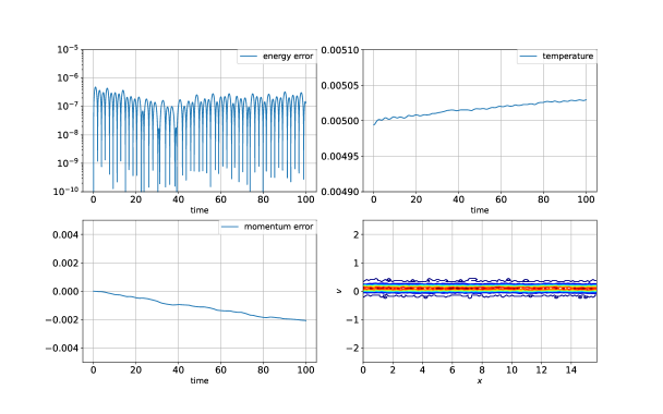
Figure 1: Finite grid instability of MB-VP by Hamiltonian splitting method. Time evolution of total energy error, temperature of ions, momentum error, and contour plot of $x-v$ at $t=100$.

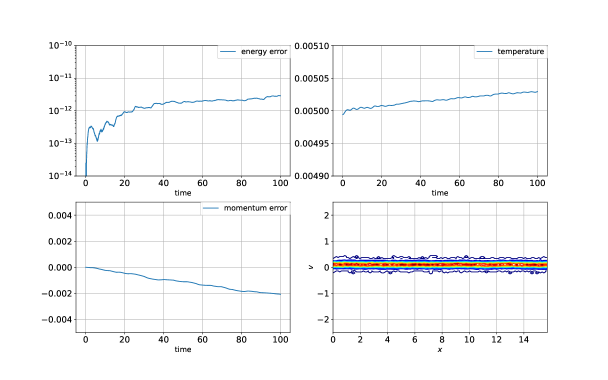
Figure 2: Finite grid instability of MB-VP by discrete gradient method. Time evolution of total energy error, temperature of ions, momentum error, and contour plot of $x-v$ at $t=100$.

5.2 Nonlinear Landau damping

Here we simulate ion Landau damping by one dimensional simulations. Initial distribution function is

$$f=\frac{1}{\pi^{\frac{1}{2}}v_{T}^{\frac{1}{2}}}(1+0.5\cos(0.5x))\exp\left({-\frac{v^{2}}{v_{T}^{2}}}\right).$$

Computational parameters are: grid number 65, domain size $[0,4\pi]$, time step size $\Delta t=0.05$, final computation time $40$, $v_{T}=1.4142$, total particle number $10^{5}$. See the numerical results with large $T_{e}=100$ in Fig. 3-4 by Hamiltonian splitting method (7) and discrete gradient method (8). As $T_{e}$ is large, the term $\exp(\phi/T_{e})$ is close to 1, the solution of MB-VP (1) is close to the solution of F-VP (with static electron density as 1). In Fig. 3-4, we observe the nonlinear Landau damping. The time evolution of energy component $\frac{1}{2}\int|\nabla\phi|^{2}\mathrm{d}{x}$ decays exponentially initially, and the result given by MB-VP is very close to the result (analytical decay rate is 0.2854) given by F-VP before time $T=10$. $\frac{1}{2}\int|\nabla\phi|^{2}\mathrm{d}{x}$ oscillates when $t\in[10,30]$, then grows exponentially with time when $t\in[30,40]$ with a rate close to 0.086671 (obtained from the dispersion relation of F-VP). For Hamiltonian splitting method, energy error is about $10^{-2}$ in the initial time, then it saturates after $t=10$ at the level of $10^{-4}$. Discrete gradient method gives a smaller total energy error about $10^{-11}$, and similar behaviors of electric energy and kinetic energy are presented. The errors of neutrality given by both numerical methods are at the levels of machine precision. The contour plots of the distribution function given by schemes (7) and (8) are presented in Fig. 5, from which we can see very fine structures (the so-called filamentation phenomena) appear.

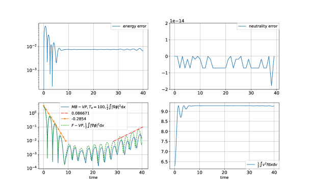
Figure 3: Nonlinear Landau damping of MB-VP with $T_{e}=100$ by Hamiltonian splitting method. Time evolution of total energy error, discrete neutrality error, electric energy $\frac{1}{2}\int|\nabla\phi|^{2}\mathrm{d}x$, and ion kinetic energy $\frac{1}{2}\int v^{2}f\mathrm{d}x\mathrm{d}v$.

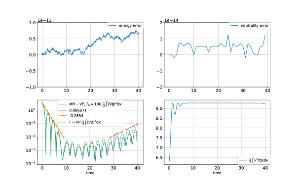
Figure 4: Nonlinear Landau damping of MB-VP with $T_{e}=100$ by discrete gradient method. Time evolution of total energy error, discrete neutrality error, electric energy $\frac{1}{2}\int|\nabla\phi|^{2}\mathrm{d}x$, and ion kinetic energy $\frac{1}{2}\int v^{2}f\mathrm{d}x\mathrm{d}v$.

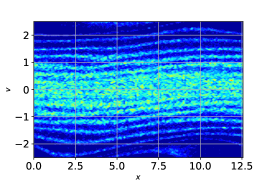
Figure 5: Contour plot of distribution function at $T=40$. Left figure: results given by Hamiltonian splitting method; Right figure: results given by discrete gradient method.

5.3 Two-stream instability

Finally, we simulate a process about instability: two-stream instability, which happens when there are two counter-streaming ion beams in a warm electron background. The initial distribution function is

$$f=\frac{1}{\pi^{\frac{1}{2}}v_{T}^{\frac{1}{2}}}\left(0.5\exp\left({-\frac{|v-v_{0}|^{2}}{v_{T}^{2}}}\right)+0.5\exp\left({-\frac{|v+v_{0}|^{2}}{v_{T}^{2}}}\right)\right).$$

Computational parameters are: grid number 32, domain size $[0,5\pi]$, time step size $\Delta t=0.01$, final computation time $40$, $v_{T}=0.1$, $T_{e}=10$, total particle number $10^{5}$, and $v_{0}=0.4$. Numerical results given by schemes (7) and (8) are presented in Fig. 6. We can see that there is an exponential growth of the second Fourier mode of $\phi$ with time, which indicates that the instabilities happen during the simulations and is consistent with the analytical rate $0.2492$ obtained by solving the following linear dispersion relation given in [32],

$$1+\frac{1}{k^{2}\lambda_{e}^{2}}=\frac{1}{2k^{2}\lambda_{i}^{2}}\left(Z^{\prime}\left(\frac{\omega-kv_{0}}{kv_{T}}\right)+Z^{\prime}\left(\frac{\omega+kv_{0}}{kv_{T}}\right)\right),\ \lambda_{e}=\sqrt{T_{e}},\ \lambda_{i}=\sqrt{T_{i}}.$$

Energy errors of scheme (7) and (8) are about $10^{-4}$ and $10^{-11}$, respectively, which validate the good conservation properties of the two schemes. Also the neutrality errors given by the two schemes are at the levels of machine precision. Similar vortex structures in $x-v$ contour plots are given by schemes (7) and (8).

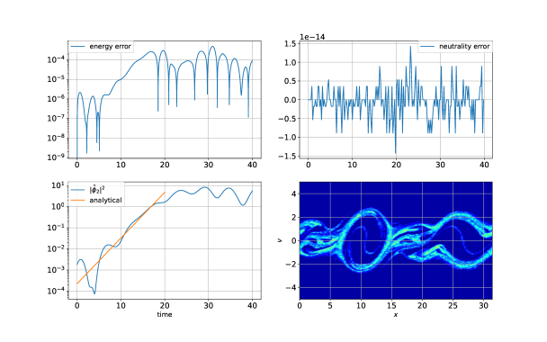
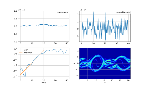
Figure 6: Two-stream instability (a): results given by Hamiltonian splitting method; (b): results given by discrete gradient method.

6 Conclusion

In this paper, we consider the structure-preserving discretizations of the Vlasov–Poisson system with Maxwell–Boltzmann electrons. The same numerical schemes are derived by discretizing either the variational action integral or the Poisson bracket. Energy and other invariants, such as momentum are conserved with small errors, which are presented in the numerical section.

We can also use finite element methods or Fourier spectral methods to discretize the electrostatic potential, and use delta functions to approximate the distribution function as [3], see more details about this in the appendix. The cases with other kinds of boundary conditions and external electromagnetic fields can also be considered in future works.

7 Appendix

Distribution function $f$ is approximated using $\delta$ functions, i.e,

$$f({x},{v},t)\approx f_{h}({x},{v},t)=\sum_{k=1}^{N_{p}}w_{k}\delta({x}-{x}_{k})\delta({v}-{v}_{k}),$$

where $N_{p}$ is the total particle number, and $w_{k}$, ${x}_{k}$, and ${v}_{k}$ are the weight, position, and velocity for $k$-th particle. We discretize $\phi$ by finite element method, i.e.

$$\phi_{h}={\boldsymbol{\Lambda}}\cdot{\boldsymbol{\phi}},$$

where the vectors ${\boldsymbol{\Lambda}}$ and ${\boldsymbol{\phi}}$ contain all basis functions and finite element coefficients. The Poisson–Boltzmann equation is discretized in weak formulation as

$$\underbrace{\int\partial_{x}\phi_{h}\partial_{x}\Lambda_{i}\mathrm{d}{x}}_{=\mathbb{M}{\boldsymbol{\phi}}}+\underbrace{\int n_{0}\exp\left({\frac{\phi_{h}}{T_{e}}}\right)\Lambda_{i}\mathrm{d}{x}}_{\approx\sum_{j=1}^{N}w_{j}n_{0}({x}_{j})\exp\left({\frac{\phi_{h}({x}_{j})}{T_{e}({x}_{j})}}\right)\Lambda_{i}({x}_{j})}=Z\sum_{k=1}^{N_{p}}w_{k}\Lambda_{i}({x}_{k}),$$ (11)

where ${x}_{j}$ is the $j$-th quadrature point, $w_{j}$ is the corresponding quadrature weight, and $\mathbb{M}_{ij}=\int\partial_{x}\Lambda_{i}\partial_{x}\Lambda_{j}\mathrm{d}{x}$.
We approximate variational action integral (2) as

$$\mathcal{A}_{h}({\mathbf{X}},{\boldsymbol{\phi}})=\sum_{k=1}^{N_{p}}w_{k}\left(\frac{1}{2}\dot{x}_{k}^{2}-Z\phi_{n}({x}_{k})\right)+{\boldsymbol{\phi}}^{\top}\mathbb{M}{\boldsymbol{\phi}}+\sum_{j=1}^{N}w_{j}n_{0}({x}_{j})T_{e}({x}_{j})\exp\left({\phi_{h}({x}_{j})/T_{e}({x}_{j})}\right).$$ (12)

Hamiltonian is discretized as

$$H=\frac{1}{2}\sum_{k=1}^{N_{p}}w_{k}{v}_{k}^{2}-\frac{1}{2}{\boldsymbol{\phi}}^{\top}\mathbb{M}{\boldsymbol{\phi}}+Z\sum_{k=1}^{N_{p}}w_{k}{\boldsymbol{\Lambda}}({x}_{k})\cdot{\boldsymbol{\phi}}-\sum_{j=1}^{N}w_{j}T_{e}({x}_{j})n_{0}({x}_{j})\exp\left({\frac{\phi_{h}({x}_{j})}{T_{e}({x}_{j})}}\right).$$ (13)

From [3], the bracket is discretized as

$$\{F,G\}_{h}=\sum_{k=1}^{N_{p}}\frac{1}{w_{k}}\left(\partial_{x_{k}}F\partial_{v_{k}}G-\partial_{x_{k}}G\partial_{v_{k}}F\right).$$ (14)

Both the variations of (12) and the discrete Poisson bracket (14) with Hamiltonian (13) give the following Hamiltonian ODE,

$$\dot{x}_{k}=\frac{1}{w_{k}}\partial_{v_{k}}H,\quad\dot{v}_{k}=-\frac{1}{w_{k}}\partial_{x_{k}}H,$$ (15)

Similarly, for the cases with periodic boundary conditions, we can prove that the neutrality condition holds in a weak sense, i.e.,

$$\sum_{j=1}^{N}w_{j}n_{0}({x}_{j})\exp\left({\frac{\phi_{h}({x}_{j})}{T_{e}({x}_{j})}}\right)\Lambda_{i}({x}_{j})=Z\sum_{k=1}^{N_{p}}w_{k}\Lambda_{i}({x}_{k}),\quad\forall i=1,\cdots,N.$$

References

- [1] Hu Y, Wang J. Expansion of a collisionless hypersonic plasma plume into a vacuum. Physical Review E, 2018, 98(2): 023204.
- [2] Valentini F, Califano F, Perrone D, Pegoraro F, Veltri P. Excitation of nonlinear electrostatic waves with phase velocity close to the ion-thermal speed. Plasma Physics and Controlled Fusion, 2011, 53(10): 105017.
- [3] Kraus M, Kormann K, Morrison P J, Sonnendrücker E. GEMPIC: geometric electromagnetic particle-in-cell methods. Journal of Plasma Physics, 2017, 83(4).
- [4] Xiao J, Qin H, Liu J, He Y, Zhang R, Sun Y. Explicit high-order non-canonical symplectic particle-in-cell algorithms for Vlasov–Maxwell systems. Physics of Plasmas, 2015, 22(11): 112504.
- [5] He Y, Sun Y, Qin H, et al. Hamiltonian particle-in-cell methods for Vlasov-Maxwell equations. Physics of Plasmas, 2016, 23(9): 092108.
- [6] Feng K, Qin M. Symplectic geometric algorithms for Hamiltonian systems. Berlin: Springer, 2010.
- [7] Hairer E, Lubich C, Wanner G. Geometric Numerical Integration: Structure-Preserving Algorithms for Ordinary Differential Equations, vol. 31, Springer Science & Business Media, 2006.
- [8] Qin H, Liu J, Xiao J, Zhang R, He Y, Wang Y, Sun Y, Burby J W, Ellison L, Zhou Y. Canonical symplectic particle-in-cell method for long-term large-scale simulations of the Vlasov–Maxwell equations. Nuclear Fusion, 2015, 56(1): 014001.
- [9] Rambo P W. Finite-grid instability in quasineutral hybrid simulations. Journal of Computational Physics, 1995, 118(1): 152-158.
- [10] Li Y, Campos Pinto M, Holderied F, Possanner S, Sonnendrücker E. Geometric Particle-In-Cell discretizations of a plasma hybrid model with kinetic ions and mass-less fluid electrons[J]. arXiv preprint arXiv:2304.01891, 2023.
- [11] Li Y, Holderied F, Possanner S, Sonnendrücker E. Numerical simulations for a hybrid model of kinetic ions and mass-less fluid electrons in canonical formulations. arXiv preprint arXiv:2301.10097, 2023.
- [12] Xiao J, Qin H. Field theory and a structure-preserving geometric particle-in-cell algorithm for drift wave instability and turbulence. Nuclear Fusion, 2019, 59(10): 106044.
- [13] Gu A, He Y, Sun Y. Hamiltonian Particle-in-Cell methods for Vlasov–Poisson equations. Journal of Computational Physics, 2022, 467: 111472.
- [14] Degond P, Liu H, Savelief D, et al. Numerical approximation of the Euler-Poisson-Boltzmann model in the quasineutral limit. Journal of Scientific Computing, 2012, 51: 59-86.
- [15] Chen L, Holst M J, Xu J. The finite element approximation of the nonlinear Poisson–Boltzmann equation. SIAM journal on numerical analysis, 2007, 45(6): 2298-2320.
- [16] Yin P, Huang Y, Liu H. An iterative discontinuous Galerkin method for solving the nonlinear Poisson Boltzmann equation. Communications in Computational Physics, 2014, 16(2): 491-515.
- [17] Yin P, Huang Y, Liu H. Error estimates for the iterative discontinuous galerkin method to the nonlinear Poisson–Boltzmann equation. Communications in computational physics, 2018, 23(1).
- [18] Xu Z, Cai W. Fast analytical methods for macroscopic electrostatic models in biomolecular simulations. SIAM review, 2011, 53(4): 683-720.
- [19] Lu B Z, Zhou Y C, Holst M J, McCammon J A. Recent progress in numerical methods for the Poisson–Boltzmann equation in biophysical applications. Commun Comput Phys, 2008, 3(5): 973-1009.
- [20] Gonzalez O. Time integration and discrete Hamiltonian systems. Journal of Nonlinear Science, 1996, 6(5), 449-467.
- [21] Cheng C Z, Knorr G. The integration of the Vlasov equation in configuration space. Journal of Computational Physics, 1976, 22(3): 330-351.
- [22] Sonnendrücker E, Roche J, Bertrand P, Ghizzo A. The semi-Lagrangian method for the numerical resolution of the Vlasov equation. Journal of computational physics, 1999, 149(2): 201-220.
- [23] Birdsall C K, Langdon A B. Plasma physics via computer simulation. CRC press, 2018.
- [24] Hockney R W, Eastwood J W. Computer simulation using particles. CRC Press, 2021.
- [25] Heath R E, Gamba I M, Morrison P J, Michler C. A discontinuous Galerkin method for the Vlasov–Poisson system. Journal of Computational Physics, 2012, 231(4): 1140-1174.
- [26] Manzini G, Delzanno G L, Vencels J, Markidis S. A Legendre–Fourier spectral method with exact conservation laws for the Vlasov–Poisson system. Journal of Computational Physics, 2016, 317: 82-107.
- [27] Silin I, Sydora R, Sauer K. Electron beam-plasma interaction: Linear theory and Vlasov-Poisson simulations. Physics of plasmas, 2007, 14(1): 012106.
- [28] Bychenkov V Y, Novikov V N, Batani D, et al. Ion acceleration in expanding multispecies plasmas. Physics of Plasmas, 2004, 11(6): 3242-3250.
- [29] Bardos C, Golse F, Nguyen T T, Sentis R. The Maxwell–Boltzmann approximation for ion kinetic modeling. Physica D: Nonlinear Phenomena, 2018, 376: 94-107.
- [30] Holderied F, Possanner S, Wang X. MHD-kinetic hybrid code based on structure-preserving finite elements with particles-in-cell. Journal of Computational Physics, 2021, 433: 110143
- [31] Webb S D. A spectral canonical electrostatic algorithm. Plasma Physics and Controlled Fusion, 2016, 58(3): 034007.
- [32] Okuda H, Dawson J M, Lin A T, Lin C C. Quasi-neutral particle simulation model with application to ion wave propagation. The Physics of Fluids, 1978, 21(3): 476-482.