Self-learning Monte Carlo with equivariant Transformer

Abstract

Machine learning and deep learning have revolutionized computational physics, particularly the simulation of complex systems. Equivariance is essential for simulating physical systems because it imposes a strong inductive bias on the probability distribution described by a machine learning model. However, imposing symmetry on the model can sometimes lead to poor acceptance rates in self-learning Monte Carlo (SLMC). Here, we introduce a symmetry equivariant attention mechanism for SLMC, which can be systematically improved. We evaluate our architecture on a spin-fermion model (i.e., double exchange model) on a two-dimensional lattice. Our results show that the proposed method overcomes the poor acceptance rates of linear models and exhibits a similar scaling law to large language models, with model quality monotonically increasing with the number of layers. Our work paves the way for the development of more accurate and efficient Monte Carlo algorithms with machine learning for simulating complex physical systems.

Introduction. The fields of machine learning and deep learning are rapidly transforming computational physics, with profound implications for fields such as condensed matter, particle physics, and cosmology. This progress has been particularly notable since 2016, with the emergence of innovative techniques catalyzed by the rise of deep learning.

One of the most promising applications of machine learning in computational physics is the use of trainable models in Monte Carlo methods. The Self-learning Monte Carlo (SLMC) method, developed for electron systems in condensed matter [1], has been widely used in strongly correlated electron systems [2, 3, 4, 5], molecular dynamics [6, 7, 8], and lattice quantum chromodynamics (QCD) [9, 10]. SLMC constructs effective models to generate the Boltzmann weight by means of machine learning from gathered original Markov chains. Moreover, it has been used in flow-based sampling algorithms to realize field theoretical distributions using trivial distribution and Jacobian [11, 12, 13, 14, 15, 16, 17, 18, 19, 20].

The Transformer architecture, which debuted as a translation model [21], has since been applied to a wide range of problems, including image recognition [22], protein folding computations [23], and foundation models such as GPT (Generative Pre-trained Transformer) [24, 25, 26, 27]. Transformer models exhibit a favorable scaling law for model capacity, meaning that their performance increases in proportion to the size of the input data [28, 29].

The symmetry of a system is essential to its description in physics. In machine learning, the imposition of an inductive bias in probability models corresponds to the symmetry of the system [30, 31]. For example, convolutional layers for neural nets respect translational symmetry, which helps in image recognition. This concept has been generalized to general symmetries [32], and is applied to a large class of models in physics [11, 12, 13, 14, 15, 16, 17, 18, 19].

In this study, we introduce the use of an equivariant transformer within SLMC, exemplified by its application to a two-dimensional spin-fermion model (i.e., double exchange model). Leveraging the extensive capacity of the attention layer, we successfully construct an effective model of the system using the equivariant transformer. We find that the model with the attention blocks overcomes the poor acceptance rates of linear models and exhibits a similar scaling law as in large language models.

Double exchange model. In this letter, we focus on the double exchange model on the two-dimensional square lattice to examine the SLMC with equivalent Transformer. We consider a two-dimensional double exchange (DE) model with classical spins [33, 2, 34]. The DE model (spin fermion model) is defined as

$$H=-t\sum_{\alpha,\langle i,j\rangle}(\hat{c}^{\dagger}_{i\alpha}\hat{c}_{j\alpha}+{\rm h.c.})\\ +\frac{J}{2}\sum_{i}{\bm{S}}_{i}\cdot\hat{\bm{\sigma}}_{i}-\mu\sum_{\alpha,i}\hat{c}_{i\alpha}^{\dagger}\hat{c}_{j\alpha},$$ (1)

where ${\bm{S}}_{i}$ is the classical Heisenberg spins on the $i$-th site, $t$ is the hopping constant, $\hat{c}_{i\alpha}^{\dagger}$ ($\hat{c}_{i\alpha}$) is the fermionic creation (annihilation) operator at the $i$-th site for fermion with spin $\alpha\in\{\uparrow,\downarrow\}$, $\langle i,j\rangle$ are the pairs of nearest neighbors, $J$ is the interaction strength between the classical spins and the electrons, and the Pauli matrices are defined as $[\hat{\bm{\sigma}}_{i}]_{\gamma}\equiv\hat{c}_{i\alpha}^{\dagger}\sigma_{\alpha\beta}^{\gamma}\hat{c}_{i\beta}$ ($\gamma=x,y,z$). We consider the hopping constant $t$ as the unit of energy. We adopt the periodic boundary condition on $N_{x}\times N_{y}$ site system. The total number of the sites is $N\equiv N_{x}N_{y}$. The Hamiltonian has $O(3)$ rotational symmetry in the spin sector and discrete translational invariance.

The partition function of the model is expressed as

$${\cal Z}=\sum_{\{{\bm{S}}\}}W(\{{\bm{S}}\}),$$ (2)

where $W(\{{\bm{S}}\})\equiv\prod_{n}(1+e^{-\beta(\mu-E_{n}(\{{\bm{S}}\}))})$ is the Boltzmann weight with as a spin configuration ${\{\bm{S}}\}$ and $E_{n}(\{{\bm{S}}\})$ is the $n$-th eigenvalue of the Hamiltonian. A standard method to simulate this system is the Markov chain Monte Carlo (MCMC) method. In the DE model, however, computational complexity is huge due to a fermion determinant for itinerant electrons, since a full diagonalization is needed to estimate the fermion determinant for given spin configurations for each Monte Carlo (MC) step. Many alternative algorithms to simulate electrons coupled to classical spin fields have been developed [35, 36, 37, 38, 39, 33, 2, 4].

We can calculate the magnitude of the average magnetization and staggered magnetization

$$|{\bm{M}}| =\frac{1}{Z}\sum_{\{{\bm{S}}\}}W(\{{\bm{S}}\})\left\|\frac{1}{N}\sum_{i}{\bm{S}}_{i}\right\|,$$ (3)

$$|{\bm{M}}_{s}| =\frac{1}{Z}\sum_{\{{\bm{S}}\}}W(\{{\bm{S}}\})\left\|\frac{1}{N}\sum_{i}(-1)^{\sum_{j=1}^{d}x_{j}}{\bm{S}}_{i}\right\|,$$ (4)

where $x_{j}$ in the sum $\sum_{j}^{d}x_{j}$ indicates the site index in the $j$-th dimension. According to Ref. [34], the parameters used in this letter favor antiferromagnetic order at low temperatures and this behavior should be captured by the staggered magnetization.

Self-learning Monte Carlo Method. The physical observable such as the magnetization can be calculated by the MCMC. In the Monte Carlo method, we have to generate a spin configuration $\{{\bm{S}}\}$ with a probability distribution $W(\{{\bm{S}}\})$. By constructing a Markov chain that has the desired distribution as its equilibrium distribution:

$$\{{\bm{S}}\}_{1}\rightarrow\{{\bm{S}}\}_{2}\rightarrow\cdots\rightarrow\{{\bm{S}}\}_{i}\rightarrow\cdots,$$ (5)

we can obtain a sample of the desired distribution by observing the chain after a number of steps. We introduce the condition of the detailed balance expressed as

$$W(\{{\bm{S}}\})P(\{{\bm{S}}^{\prime}\}|\{{\bm{S}}\}) =W(\{{\bm{S}}^{\prime}\})P(\{{\bm{S}}\}|\{{\bm{S}}^{\prime}\}),$$ (6)

where $P(\{{\bm{S}}^{\prime}\}|\{{\bm{S}}\})$ is the transition probability from another configuration $\{{\bm{S}}\}$ to a configuration $\{{\bm{S}}^{\prime}\}$. In the Metropolis-Hastings approach, the transition probability is separated in two substeps:

$$P(\{{\bm{S}}^{\prime}\}|\{{\bm{S}}\}) =g(\{{\bm{S}}^{\prime}\}|\{{\bm{S}}\})A(\{{\bm{S}}^{\prime}\},\{{\bm{S}}\}),$$ (7)

where the proposal distribution $g(\{{\bm{S}}\}^{\prime}|\{{\bm{S}}\})$ is the conditional probability of proposing a configuration $\{{\bm{S}}^{\prime}\}$ when a configuration $\{{\bm{S}}\}$ is given, and the acceptance ratio $A(\{{\bm{S}}^{\prime}\},\{{\bm{S}}\})$ is the probability to accept the proposed configuration $A(\{{\bm{S}}^{\prime}\},\{{\bm{S}}^{\prime}\})$. The Markov chain that has the desired distribution $W(\{{\bm{S}}\})$ is obtained when the acceptance ratio is given as

$$A(\{{\bm{S}}^{\prime}\},\{{\bm{S}}\})={\rm min}\left(1,\frac{W(\{{\bm{S}}^{\prime}\})}{W(\{{\bm{S}}\})}\frac{g(\{{\bm{S}}\}|\{{\bm{S}}^{\prime}\})}{g(\{{\bm{S}}^{\prime}\}|\{{\bm{S}}\})}\right).$$ (8)

One can design various kinds of the Monte Carlo method based on Eq. (8). The most simple update method is so-called local update, where the spin configuration is updated locally. A single site is randomly chosen in the current configuration and a new configuration is proposed by changing the orientation of the classical spin. Although it is easy to implement the local update in various kinds of systems, the computational cost is usually high because the autocorrelation time is long. We note that the hybrid Monte Carlo method is known as the one of the good update methods, which is widely used in lattice QCD.

In MCMC, the proposal probability $g(\{{\bm{S}}^{\prime}\}|\{{\bm{S}}\})$ can be designed to increase the acceptance ratio $A(\{{\bm{S}}^{\prime}\},\{{\bm{S}}\})$. If the ratio of the proposal probability $\frac{g(\{{\bm{S}}\}\{{\bm{S}}^{\prime}\})}{g(\{{\bm{S}}^{\prime}\}\{{\bm{S}}\})}=\frac{W(\{{\bm{S}}\})}{W(\{{\bm{S}}^{\prime}\})}$, the new configuration $\{{\bm{S}}^{\prime}\}$ is always accepted because of $A(\{{\bm{S}}^{\prime}\},\{{\bm{S}}\})=1$. In the SLMC, we introduce the another Markov chain with the probability $W_{\rm prop}(\{{\bm{S}}\})$. The detailed balance condition is given as

$$W_{\rm prop}(\{{\bm{S}}\})P_{\rm prop}(\{{\bm{S}}^{\prime}\}|\{{\bm{S}}\})\\ =W_{\rm prop}(\{{\bm{S}}^{\prime}\})P_{\rm prop}(\{{\bm{S}}\}|\{{\bm{S}}^{\prime}\}).$$ (9)

On the proposal Markov chain, the configuration $\{{\bm{S}}^{\prime}\}$ is obtained by the random walk from $\{{\bm{S}}\}$. The proposal probability $P_{\rm prop}(\{{\bm{S}}^{\prime}\}|\{{\bm{S}}\})$ can be regarded as the conditional probability $g(\{{\bm{S}}^{\prime}\}|\{{\bm{S}}\})$ on the original Markov chain. Thus, the acceptance ratio in the SLMC is given as

$$A(\{{\bm{S}}^{\prime}\},\{{\bm{S}}\})={\rm min}\left(1,\frac{W(\{{\bm{S}}^{\prime}\})}{W(\{{\bm{S}}\})}\frac{W_{\rm prop}(\{{\bm{S}}\})}{W_{\rm prop}(\{{\bm{S}}^{\prime}\})}\right).$$ (10)

If we can design the proposal Markov chain whose probability is equal to that of the original Markov chain, the proposed spin configuration $\{{\bm{S}}^{\prime}\}$ is always accepted.

We introduce an effective model for making a proposal in the Markov chain with the probability $W_{\rm eff}(\{{\bm{S}}\})\equiv W_{\rm prop}(\{{\bm{S}}\})$. The probability $W_{\rm eff}(\{{\bm{S}}\})$ can be written as

$$W_{\rm eff}(\{{\bm{S}}\})=\exp\left[-\beta H_{\rm eff}(\{{\bm{S}}\},T)\right],$$ (11)

where the effective Hamiltonian $H_{\rm eff}(\{{\bm{S}}\},T)$ is a real scalar. We note that the effective Hamiltonian generally depends on the temperature. The average acceptance ratio $\langle A\rangle$ can be estimated by [3]

$$\langle A\rangle=e^{-\sqrt{{\rm MSE}}},$$ (12)

with the mean squared error (MSE) between the original and effective models:

$${\rm MSE}=\frac{1}{N_{\{{\bm{S}}\}}}\sum_{\{{\bm{S}}\}}\left|\log W(\{{\bm{S}}\})-\log W_{\rm eff}(\{{\bm{S}}\})\right|^{2},$$ (13)

where $N_{\{{\bm{S}}\}}$ is the number of spin configurations.

Effective models In previous works about the double exchange model [2, 4], the linear model expressed as

$$H_{\rm eff}^{\rm Linear}=E_{0}-\sum_{\langle i,j\rangle_{n}}J_{n}^{\rm eff}{\bm{S}}_{i}\cdot{\bm{S}}_{j}.$$ (14)

is used as the effective model. If the interaction strength $J$ is weak, the Ruderman-Kittel-Kasuya-Yoshida (RKKY) interaction is derived by the perturbation theory [40, 41, 42]. With the use of the SLMC, we can fit the effective coupling $J_{n}^{\rm eff}$ far from the weak coupling regime and the functional form of $J_{n}^{\rm eff}$ is similar to the RKKY interaction [2, 4].

Let us construct general effective model that is an extension of the linear model. A general effective model is a functional of all spins:

$$H=f({\bm{S}}).$$ (15)

Here, we regard the classical spin field as the matrix whose matrix element is defined as

$$S_{i\mu}\equiv[{\bm{S}}_{i}]_{\mu}.$$ (16)

We consider that the general effective model should be invariant with respect to rotations in spin space, spatial reflections, and translations in real space. By introducing the spin rotation matrix $R$ which rotates all spins in spin space, the effective model should satisfy the following relation:

$$f({\bm{S}}R)=f({\bm{S}}).$$ (17)

To satisfy the rotational invariance, we introduce a Gram matrix [43]:

$$G({\bm{S}})\equiv{\bm{S}}{\bm{S}}^{T}.$$ (18)

Here, the Gram matrix is rotation-invariant, the size of the Gram matrix is the number of sites $N$ and the matrix element is defined as

$$[G({\bm{S}})]_{ij}={\bm{S}}_{i}\cdot{\bm{S}}_{j}.$$ (19)

According to Ref. [43], if the Gram matrix of two spin field are equal, their geometrical structures are also the same. Thus, the general effective model should be a functional of the Gram matrix:

$$H=f_{G}(G({\bm{S}})).$$ (20)

In terms of the functional of the Gram matrix, we rewrite the linear model in Eq. (14). We introduce the local operator for spins:

$$\hat{A}{\bm{S}} \equiv{\bm{S}}^{\hat{A}},$$ (21)

where the matrix element of ${\bm{S}}^{\hat{A}}$ is defined as

$$S_{i\mu}^{\hat{A}} \equiv\sum_{\langle i,j\rangle_{n}}A_{n}S_{j\mu}.$$ (22)

Since the local operation does not rotate spins in spin space, $\hat{A}$ is an equivariant with respect to rotations in spin space:

$$\hat{A}({\bm{S}}R)={\bm{S}}^{\hat{A}}R.$$ (23)

Here, a function $f:X\rightarrow Y$ is equivariant with respect to a group $G$ that acts on $X$ and $Y$ if:

$$D_{Y}[g]f(x)=f(D_{X}[g]x),\>\>\forall g\in G,\forall x\in X,$$ (24)

where $D_{X}[g]$ and $D_{Y}[g]$ are the representations of the group element $g$ in the spaces $X$ and $Y$, respectively. Equivariant networks have been used in various kinds of fields such as point cloud processing [44, 45] and machine-learning molecular dynamics [46, 47].

With the use of the above definitions, the linear effective model is rewritten as

$$H_{\rm eff}^{\rm Linear}={\rm Tr}\left[{\bm{S}}(\hat{J}{\bm{S}})^{\top}\right]+E_{0}.$$ (25)

With the use of the Gram matrix, this model becomes

$$H_{\rm eff}^{\rm Linear}={\rm Tr}\left[\check{J}G({\bm{S}})\right]+E_{0},$$ (26)

where $\check{J}$ is a $N\times N$ matrix.

To extend the linear model, we introduce the effective spin field ${\bm{S}}_{\rm eff}$ defined as

$${\bm{S}}_{\rm eff}=\check{M}(G({\bm{S}})){\bm{S}},$$ (27)

where $\check{M}(G({\bm{S}}))$ is a $N\times N$ matrix and ${\bm{S}}_{\rm eff}$ is equivarient with respect to spin rotations since the Gram matrix is rotational invariant. With the use of this effective spin field, we propose the effective model expressed as

$$H_{\rm eff}^{\rm NN}={\rm Tr}\left[{\bm{S}}_{\rm eff}(\hat{J}{\bm{S}}_{\rm eff})^{\top}\right]+E_{0},$$ (28)

which is a functional of the Gram matrix with respect to ${\bm{S}}_{\rm eff}$.

In this letter, we construct the effective spin field that consists of the neural networks with multiple attention layers. In this work, we note index of layers as $l=1,2,\cdots,L$.

The network architecture is expressed by

$${\bm{S}}^{(0)} \equiv{\bm{S}},$$ (29)

$${\bm{S}}^{(l)} \equiv{\cal N}\left({\bm{S}}^{(l-1)}+{\rm SelfAttention}_{{\bm{\theta}}^{(l)}}^{\rm spin}({\bm{S}}^{(l-1)})\right),$$ (30)

$${\bm{S}}_{\rm eff} ={\bm{S}}^{(L)}.$$ (31)

${\rm SelfAttention}_{{\bm{\theta}}^{(l)}}^{\rm spin}({\bm{S}}^{(l-1)})$ is a neural network map between spin configurations, which will be explained following. ${\bm{\theta}}^{(l)}$ represents a set of network trainable parameters in $l$-th layer. ${\cal N}({\bm{S}})$ normalizes the spin vector on each lattice site,

$${\cal N}({\bm{S}}_{i})=\frac{{\bm{S}}_{i}}{\|{\bm{S}}_{i}\|}.$$ (32)

We call this network architecture the equivariant Transformer, which is schematically visualized in Fig. 1.

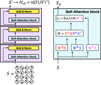
Figure 1: (Left) (Color online) Construction of effective Hamiltonian with the use of the equivariant Transformer with three of attention layers. Yellow blocks are defined by Eq. (42). We call purple blocks the attention layers. (Right) Blue blocks are equivariant attention block (See main text).

The attention block is an essential component of the transformer neural networks (See, Supplemental Material). In our system with classical spin field, we introduce the following self-attention block:

$${\rm SelfAttention}^{\rm spin}({\bm{S}})=\check{M}{\bm{S}}^{\rm V},$$ (33)

where

$$\check{M}\equiv\sigma\left(\frac{1}{\sqrt{3}}{\bm{S}}^{{\rm Q}}{\bm{S}}^{{\rm K},\top}\right),$$ (34)

and $\sigma$ is a nonlinear activation function applied element-wisely. This can be written as

$$\left[\check{M}\right]_{ij}=\sigma\left(\frac{1}{\sqrt{3}}\sum_{\mu}S_{i\mu}^{\rm Q}S_{j\mu}^{\rm K}\right),$$ (35)

In this letter, we use the ReLU function defined as

$${\rm ReLU}(x)=\left\{\begin{array}[]{ll}0&x<0,\\ x&{\rm otherwise}\end{array}\right..$$ (38)

Here, queries, keys, and values are $N\times 3$ matrices defined as

$${\bm{S}}^{\rm Q} \equiv\hat{W}^{\rm Q}{\bm{S}},$$ (39)

$${\bm{S}}^{\rm K} \equiv\hat{W}^{\rm K}{\bm{S}},$$ (40)

$${\bm{S}}^{\rm V} \equiv\hat{W}^{\rm V}{\bm{S}}.$$ (41)

We note that the matrix $\check{M}$ is a functional of the Gram matrix with respect to ${\bm{S}}$. The local operators $\hat{W}^{\rm Q},\hat{W}^{\rm K},\hat{W}^{\rm V}$ have trainable parameters. It should be noted that the number of the trainable parameters in the local operator is usually fewer than a dozen. For example, if one considers $n$-th neighbors, the number of the trainable parameters in one local operator is only $n+1$. In terms of machine-learning community, this is called the weight sharing.

The effective spin field generated by our attention layer in Eq. (31) has the spin rotational equivariance. We show that the effective spin has also the translational operation equivariance as follows. Since the matrices $\hat{W}^{\rm Q}$, $\hat{W}^{\rm K}$ and $\hat{W}^{\rm V}$ are local operators, the spin fields ${\bm{S}}^{\rm Q}$, ${\bm{S}}^{\rm K}$ and ${\bm{S}}^{\rm V}$ are translational operation equivariant ($T{\bm{S}}^{\rm Q}=\hat{W}^{\rm Q}(T{\bm{S}})$). Here, $T$ is a translational operator. Although the matrix $\check{M}$ defined in Eq. (34) is not invariant with respect to the translational operation ($\check{M}\rightarrow T\check{M}T^{\top}$), the self-attention block in Eq. (33) is translational operation equivariant because $\check{M}{\bm{S}}^{\rm V}\rightarrow T\check{M}T^{\top}({T\bm{S}}^{\rm V})=T(\check{M}{\bm{S}}^{\rm V})$.

Model training. The trainable weights in the $l$-th layer are $\hat{W}^{{\rm Q},(l)}$, $\hat{W}^{{\rm K},(l)}$ and $\hat{W}^{{\rm V},(l)}$. The number of the trainable parameters in the local operator $\hat{W}^{\alpha}$ is $m^{\rm\alpha}$. In this letter, we consider $n$-th nearest neighbors on all attention layers so that $m^{\rm\alpha}=n+1$. There are $3(n+1)$ trainable parameters in each attention layer. As shown in Eq. (28), the trainable weights in the last layer are $\hat{J}$ and $E_{0}$. The number of the trainable parameters in $\hat{J}$ is $m_{J}+1$ since $m_{J}$-th nearest neighbors are considered in the last layer. The total number of the trainable parameters with $L$ attention layers is $3L(n+1)+m_{J}+1+1$, which is quite less than fully-connected neural networks.

We should note that the number of the trainable parameters does not depend on the system size $N$. Therefore, the effective model obtained in a smaller system can be used in larger systems without any change.

We train the effective model with $L$ attention layers, iteratively. We focus on the fact that the effective spin field with $L$ attention layers ${\bm{S}}^{{\rm eff}(L)}$ is expressed as

$${\bm{S}}^{{\rm eff}(L)}={\cal N}\left({\bm{S}}^{{\rm eff}(L-1)}+\check{M}^{(L-1)}\hat{W}^{{\rm V},(L-1)}{\bm{S}}^{{\rm eff}(L-1)}\right).$$ (42)

If the trainable weight $\check{M}^{(L-1)}$ or $\hat{W}^{{\rm V},(L-1)}$ is zero, ${\bm{S}}^{{\rm eff}(L)}$ becomes ${\bm{S}}^{{\rm eff}(L-1)}$. Because the parameter space for ${\bm{S}}^{{\rm eff}(L-1)}$ is inside the parameter space for ${\bm{S}}^{{\rm eff}(L)}$, we can use converged parameters for ${\bm{S}}^{{\rm eff}(L-1)}$ as the initial guess for ${\bm{S}}^{{\rm eff}(L)}$.

At first, we consider the linear model ($L=0$) shown in Eq. (28) where the trainable weights are only $\hat{J}$ and $E_{0}$. After the training with the linear model, we introduce the weights $\hat{W}^{{\rm Q},(l=1)}$, $\hat{W}^{{\rm K},(l=1)}$ and $\hat{W}^{{\rm V},(l=1)}$ whose matrix elements are uniform random numbers $r\in[-\epsilon,\epsilon]$. In this letter, we set $\epsilon=10^{-6}$. After the training with the effective model with $l$ attention layers, we can prepare the initial guess for the effective model with $l+1$ attention layers.

We train the effective model with the use of the SLMC. We set the total number of the Metropolis-Hastings tests with the original model $N_{\rm MC}^{\rm original}$ and the length of the proposal Markov chain $N_{\rm MC}^{\rm eff}$, where ${\bm{S}}^{{\rm eff}(L-1)}$ is the effective spin field with $L-1$ attention layers. The training procedure with the use of the SLMC is shown as follows. At first, we prepare the initial effective model. The initial guess is produced by the iterative method proposed in the previous section. Next, we produce a randomly oriented spin configuration. With the use of the MCMC with the effective model $H_{\rm eff}$, the random spin configurations are approximately thermalized. This configuration is regarded as the initial configuration $\{{\bm{S}}\}_{1}$ in terms of the SLMC. Then, we calculate the weights $W$ and $W_{\rm eff}$. The proposal configuration $\{{\bm{S}}\}_{2}$ is generated by the MCMC with the effective model. The configuration $\{{\bm{S}}\}_{2}$ is accepted if the uniform random number is smaller than the acceptance ratio $A(\{{\bm{S}}_{2}\},\{{\bm{S}}_{1}\})$. If the configuration is rejected, we use $\{{\bm{S}}\}_{1}$ as the initial configuration for the effective MCMC and try to propose new configuration $\{{\bm{S}}\}_{2}^{\prime}$. The quality of the effective model can be estimated by the average acceptance ratio in the SLMC. If the acceptance ratio in the SLMC is too low, we make $N_{\rm MC}^{\rm eff}$ smaller. In this letter, we first use $N_{\rm MC}^{\rm eff}=10$ to obtain better initial guess and set $N_{\rm MC}^{\rm eff}=100$ in the main SLMC.

To optimize the training parameters, we use Flux.jl [48], machine-learning framework written in Julia language [49]. We adopt the AdamW optimizer (the parameters are $\eta=0.001$ and $\beta=(0.9,0.999)$ as in [50]) and the size of the minibatch is 100, which means that the effective model is improved at every 100 Metropolis-Hastings tests.

Results and Discussion. We consider two-dimensional $N_{x}\times N_{y}$ square lattice. The interaction strength $J$ between the classical spins and the electrons and the chemical potential $\mu$ are set to $J=1t$ and $\mu=0$, respectively. The effective model is trained by the SLMC in the $6\times 6$ square lattice. We consider $6$-th nearest neighbors in the attention layers so that we set $m^{\rm\alpha}=n+1=7$. In the each proposal Markov chain, we adopt the local spin rotation update.

For comparison, we also perform the MCMC simulation with the original Hamiltonian. In the $6\times 6$ square lattice system, the length of the Markov chain is $2\times 10^{5}$.

Since the SLMC is the MCMC with the original Hamiltonian, the physical quantities can be calculated exactly. Over the whole temperature range, we use same effective model trained at $T=0.05t$.

As shown in Fig. 2, the SLMC with effective models successfully reproduces the physical quantities obtained by the original model. There is the anti-ferromagnetic order in low temperature regime. We confirm that the autocorrelation time in the SLMC is drastically shorter than that in the original MCMC (See, the Supplemental Material).

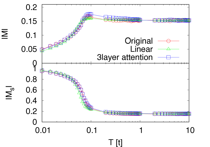
Figure 2: (Color online) Magnitude of average magnetization and staggered magnetization for a two-dimensional system with $6\times 6=36$ lattice sites. For each temperature, we generate $2\times 10^{5}$ samples using exact diagonalization (red circles), $5000$ samples using SLMC with the linear model (green triangles) and the effective model with 3layer attention (blue squares).

Next, we show that our model with attention layers can capture the long-range interaction. In this section, we consider the nearest neighbors in the last layer ($m_{J}=1$). Since a quality of the effective model can be estimated by the average acceptance ratio of the SLMC, we consider the layer number dependence of the acceptance ratio. The effective models are trained at $T=0.05t$ on the $6\times 6$ square lattice. We set $N_{\rm MC}^{\rm original}=3\times 10^{4}$ and $N_{\rm MC}^{\rm eff}=100$ in this section. The average acceptance ratio for the SLMC with the linear model is only about 21%, since the long-range spin-spin interaction is neglected in this model. The layer number dependence is shown in Fig. 3. The acceptance ratio becomes higher with increasing the number of attention layers. We explain the reason why the effective model with the attention layers can treat the long-range spin-spin interactions as follows. The effective model is expressed as the short-range interaction of the effective spins defined by Eq. (42). Since the matrix $\check{M}$ is a $N\times N$ matrix, the effective spin on a site $i$ can be expressed as

$${\bm{S}}^{{\rm eff}(L)}_{i}=\sum_{j=1}^{N}K_{ij}{\bm{S}}^{{\rm eff}(L-1)}_{j},$$ (43)

where $K$ is a weight as a functional of ${\{\bm{S}}^{{\rm eff}(L-1)}\}$. Therefore, even the onsite interaction ${\bm{S}}^{{\rm eff}(L)}_{i}\cdot{\bm{S}}^{{\rm eff}(L)}_{i}$ has the long-range interactions.

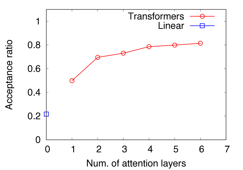
Figure 3: (Color online) Acceptance ratio in the SLMC with the effective model. We only consider the nearest neighbors in the last layer ($m_{J}=1$). A blue square indicate the acceptance ratio for the linear model. Red circles indicate models with attention blocks, with $L=1,2,3,4,5,6$ from the left.

It is known that there is the empirical scaling laws for language model performance [28]. The authors in Ref. [28] claims that performance of language models improves smoothly as we increase the model size, dataset size, and amount of compute used for training and that empirical performance has a power-law relationship with each individual factor when not bottlenecked by the other two.

We show that our model with attention blocks has also a similar scaling law. In the previous section, we discuss the layer-number dependence of the acceptance ratio (Fig. 3). With the use of Eq. (12), the MSE can be estimated from the average acceptance ratio:

$${\rm MSE}=\big{(}\log\langle A\rangle\big{)}^{2}.$$ (44)

Figure 4 shows that there is a scaling law as a functional of the number of training parameters. Here, we set $N_{\rm MC}^{\rm eff}=800$. Blue square corresponds to the estimated MSE for the linear model and red circles indicate MSE for $L=1,2,\cdots,6$ from the left. We fit only points for $L\geq 2$ to guide eyes.

We remark that in the SLMC, new training data is always generated so that the dataset size is increasing during the SLMC. This means that large data requirement for training of Attention layers can be satisfied by self-training. Moreover, we can systematically increase the number of trainable parameters in our model with adding new attention layer without loosing performance by following reason.

We discuss the origin of the scaling law that we found. We note that the origin of the scaling law in large language models is not well understood. Although we do not know the direct origin of our scaling law, we show that the MSE of the effective model can be improved with increasing the number of the attention layers. We introduce the parameter space of the effective model with $L$ attention layers ${\cal P}^{(L)}$. The parameter space with different number of the attention layers has the relation expressed as

$${\cal P}^{(0)}\in{\cal P}^{(1)}\in\cdots\in{\cal P}^{(L)}\in\cdots,$$ (45)

where ${\cal P}^{(0)}$ is the parameter space of the linear model. Let us consider the model with layer $L$ which has been optimized. In this case, the model loss has reached to the lower bound. And we add one more attention block with small random weights to the model. The model obtains additional capacity for lowering the loss. Note that, if the additional self-attention block with weight zero, the additional attention layer behaves as an identity map since it is connected with the residual connection. Thus, the MSE of the effective model with $L$ attention layers ${\rm MSE}^{(L)}$ has the following relation:

$${\rm MSE}^{(0)}\geq{\rm MSE}^{(1)}\geq\cdots\geq{\rm MSE}^{(L)}\geq\cdots.$$ (46)

This relation suggests that we can increase the number of training parameters systematically.

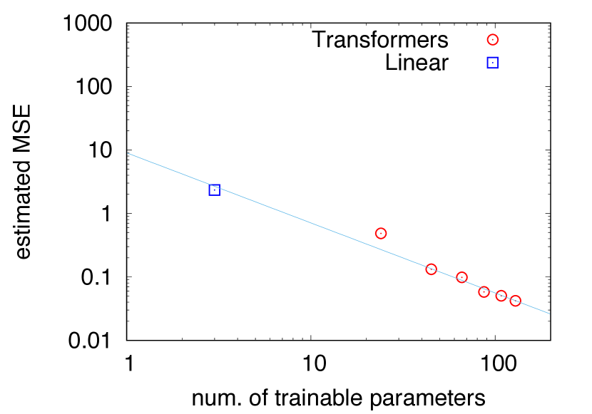
Figure 4: (Color online) Estimated MSE as a functional of the number of trainable parameters. We only consider the nearest neighbors in the last layer ($m_{J}=1$). Blue square corresponds to the estimated MSE for the linear model. Red circles indicate different models with $L=1,2,3,4,5,6$ from the left. Only points for $L\geq 2$ are fitted and the point for the linear model is not included.

Trained model can be used for simulations for an approximated system. Namely, one can perform the MCMC simulation only with the effective model. Although this simulation is not exact, the computational complexity is very low compared to the SLMC and original MC because of no estimation of the original weights. As an example, we show the results of the MCMC with the effective model in Supplemental Material.

As a future work, we need to examine volume $N$ scaling and the improvement of our symmetry equivariant attention approach in SLMC. Our attention will also be given to adapting this methodology to diverse models. We also plan to investigate and improve upon the sub-optimal volume scaling associated with the use of flow-based sampling algorithm in lattice field theory [51, 52, 53]. These strides could potentially improves acceptance ratio and elevate simulation efficiency across the board.

Summary. We introduced a new type of Transformer network with an attention layer that has spin-rotational and translational equivariance. The effective model with the attention layers is introduced in the double exchange model, where electrons are coupled to classical spins on a lattice. Using the SLMC, we generate new training data during Monte Carlo simulations to train the effective model. In the SLMC, the effective model trained at a single temperature can be applied over the whole temperature range and reproduces the antiferromagnetic phase transition. We find that the mean squared error (MSE) decreases with increasing the number of training data, following a scaling law similar to that observed in Transformer networks for large language models. Our effective model is a natural extension of the linear model and captures the nonlinear behavior of target systems.

I Supplemental Material

Attention and Transformer

Here we briefly review Transformer and Attention block [21], which have large model capacity [28]. Please see [29] for detail and recent development.

The attention layer is essential component of the transformer neural networks. The input consists of queries, keys, and values of dimension $d$. In the conventional attention layer, so-called scaled dot-product attention layer, we compute the dot products of the query with keys, divide each by $\sqrt{d}$ and apply the activation function to obtain the weights of the values. According to the Ref. [21], the conventional attention layer is defined as

$${\rm Attention}(Q,K,V)={\rm softmax}\left(\frac{QK^{T}}{\sqrt{d}}\right)V.$$ (47)

Here, $Q$,$K$ and $V$ are tensors whose size depend on system. The self-attention layer defined as

$${\rm SelfAttention}(x)={\rm Attention}(W^{\rm Q}x,W^{\rm K}x,W^{\rm V}x),$$ (48)

is used in the Transformer. Here, $W^{\rm Q}$, $W^{\rm K}$ and $W^{\rm V}$ are trainable tensors.

In the first paper [21], they develop multi-head attention, which is constructed by output of single-head output attention explained here. In this paper, we utilize single-head attention for simplicity.

Autocorrelation

We show the autocorrelation at the lowest temperature ($T=0.01t$) in Fig. 5. The SLMC reduces the autocorrelation where the number of the MC steps means the number of the calculations of the original model [2, 5, 7, 4].

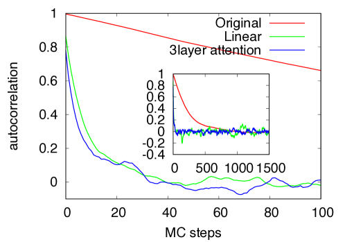
Figure 5: (Color online) Autocorrelation for magnitude of the staggered magnetization for a two-dimensional system with $6\times 6=36$ lattice sites at $T=0.01t$.

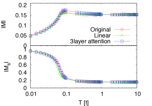
Figure 6: (Color online) Magnitude of average magnetization and staggered magnetization for a two-dimensional system with $6\times 6=36$ lattice sites without using the SLMC. For each temperature, we generate $2\times 10^{5}$ samples using exact diagonalization (red circles), the linear model (green triangles) and the effective model with 3layer attention (blue squares).

Physical observable calculated by the effective model

In the SLMC, one has to calculate the Boltzmann weights of the original Hamiltonian. However, if the effective model is similar to the original model, the MCMC only with the effective model can be used as the ”original” MCMC. As shown in Fig. 6, the MC with effective models almost reproduces the physical quantities obtained by the original model. In the case of the linear model, the staggered magnetization slighly differs from that with the original model in low temperature region.

We should note that, since the derivative of the effective model can be easily calculated by the back-propagation technique, one can use the Hybrid Monte Carlo method [35] or the Langevin Dynamics [33] with the effective model.

References

- Liu et al. [2017a] J. Liu, Y. Qi, Z. Y. Meng, and L. Fu, Self-learning monte carlo method, Physical Review B 95, 10.1103/physrevb.95.041101 (2017a).
- Liu et al. [2017b] J. Liu, H. Shen, Y. Qi, Z. Y. Meng, and L. Fu, Self-learning monte carlo method and cumulative update in fermion systems, Phys. Rev. B 95, 241104 (2017b).
- Shen et al. [2018] H. Shen, J. Liu, and L. Fu, Self-learning monte carlo with deep neural networks, Phys. Rev. B 97, 205140 (2018).
- Kohshiro and Nagai [2021] H. Kohshiro and Y. Nagai, Effective Ruderman–Kittel–Kasuya–Yosida-like interaction in diluted double-exchange model: Self-learning monte carlo approach, J. Phys. Soc. Jpn. 90, 034711 (2021).
- Nagai et al. [2017] Y. Nagai, H. Shen, Y. Qi, J. Liu, and L. Fu, Self-learning monte carlo method: Continuous-time algorithm, Phys. Rev. B 96, 161102 (2017).
- Nagai et al. [2020a] Y. Nagai, M. Okumura, K. Kobayashi, and M. Shiga, Self-learning hybrid monte carlo: A first-principles approach, Phys. Rev. B 102, 041124 (2020a).
- Nagai et al. [2020b] Y. Nagai, M. Okumura, and A. Tanaka, Self-learning monte carlo method with Behler-Parrinello neural networks, Phys. Rev. B 101, 115111 (2020b).
- Kobayashi et al. [2021] K. Kobayashi, Y. Nagai, M. Itakura, and M. Shiga, Self-learning hybrid monte carlo method for isothermal-isobaric ensemble: Application to liquid silica, J. Chem. Phys. 155, 034106 (2021).
- Nagai et al. [2023] Y. Nagai, A. Tanaka, and A. Tomiya, Self-learning monte carlo for non-abelian gauge theory with dynamical fermions, Phys. Rev. D (2023).
- Nagai and Tomiya [2021] Y. Nagai and A. Tomiya, Gauge covariant neural network for 4 dimensional non-abelian gauge theory, (2021), arXiv:2103.11965 [hep-lat] .
- Albergo et al. [2019] M. Albergo, G. Kanwar, and P. Shanahan, Flow-based generative models for markov chain monte carlo in lattice field theory, Physical Review D 100, 10.1103/physrevd.100.034515 (2019).
- Kanwar et al. [2020] G. Kanwar, M. S. Albergo, D. Boyda, K. Cranmer, D. C. Hackett, S. Racanière, D. J. Rezende, and P. E. Shanahan, Equivariant flow-based sampling for lattice gauge theory, Physical Review Letters 125, 10.1103/physrevlett.125.121601 (2020).
- Boyda et al. [2021] D. Boyda, G. Kanwar, S. Racanière, D. J. Rezende, M. S. Albergo, K. Cranmer, D. C. Hackett, and P. E. Shanahan, Sampling using gauge equivariant flows, Physical Review D 103, 10.1103/physrevd.103.074504 (2021).
- Albergo et al. [2021] M. S. Albergo, G. Kanwar, S. Racanière, D. J. Rezende, J. M. Urban, D. Boyda, K. Cranmer, D. C. Hackett, and P. E. Shanahan, Flow-based sampling for fermionic lattice field theories, Physical Review D 104, 10.1103/physrevd.104.114507 (2021).
- Hackett et al. [2021] D. C. Hackett, C.-C. Hsieh, M. S. Albergo, D. Boyda, J.-W. Chen, K.-F. Chen, K. Cranmer, G. Kanwar, and P. E. Shanahan, Flow-based sampling for multimodal distributions in lattice field theory (2021), arXiv:2107.00734 [hep-lat] .
- Albergo et al. [2022] M. S. Albergo, D. Boyda, K. Cranmer, D. C. Hackett, G. Kanwar, S. Racanière, D. J. Rezende, F. Romero-López, P. E. Shanahan, and J. M. Urban, Flow-based sampling in the lattice schwinger model at criticality, Physical Review D 106, 10.1103/physrevd.106.014514 (2022).
- Abbott et al. [2022a] R. Abbott, M. S. Albergo, D. Boyda, K. Cranmer, D. C. Hackett, G. Kanwar, S. Racanière, D. J. Rezende, F. Romero-López, P. E. Shanahan, B. Tian, and J. M. Urban, Gauge-equivariant flow models for sampling in lattice field theories with pseudofermions, Physical Review D 106, 10.1103/physrevd.106.074506 (2022a).
- Abbott et al. [2022b] R. Abbott, M. S. Albergo, A. Botev, D. Boyda, K. Cranmer, D. C. Hackett, G. Kanwar, A. G. D. G. Matthews, S. Racanière, A. Razavi, D. J. Rezende, F. Romero-López, P. E. Shanahan, and J. M. Urban, Sampling qcd field configurations with gauge-equivariant flow models (2022b), arXiv:2208.03832 [hep-lat] .
- Abbott et al. [2023] R. Abbott, M. S. Albergo, A. Botev, D. Boyda, K. Cranmer, D. C. Hackett, G. Kanwar, A. G. D. G. Matthews, S. Racanière, A. Razavi, D. J. Rezende, F. Romero-López, P. E. Shanahan, and J. M. Urban, Normalizing flows for lattice gauge theory in arbitrary space-time dimension (2023), arXiv:2305.02402 [hep-lat] .
- Tomiya and Terasaki [2022] A. Tomiya and S. Terasaki, GomalizingFlow.jl: A Julia package for Flow-based sampling algorithm for lattice field theory, (2022), arXiv:2208.08903 [hep-lat] .
- Vaswani et al. [2017] A. Vaswani, N. Shazeer, N. Parmar, J. Uszkoreit, L. Jones, A. N. Gomez, L. Kaiser, and I. Polosukhin, Attention is all you need (2017), arXiv:1706.03762 [cs.CL] .
- Dosovitskiy et al. [2021] A. Dosovitskiy, L. Beyer, A. Kolesnikov, D. Weissenborn, X. Zhai, T. Unterthiner, M. Dehghani, M. Minderer, G. Heigold, S. Gelly, J. Uszkoreit, and N. Houlsby, An image is worth 16x16 words: Transformers for image recognition at scale (2021), arXiv:2010.11929 [cs.CV] .
- Jumper et al. [2021] J. Jumper, R. Evans, A. Pritzel, et al., Highly accurate protein structure prediction with alphafold, Nature 596, 583 (2021).
- Radford et al. [2018] A. Radford, K. Narasimhan, T. Salimans, and I. Sutskever, Improving language understanding by generative pre-training, (2018).
- Radford et al. [2019] A. Radford, J. Wu, R. Child, D. Luan, D. Amodei, and I. Sutskever, Language models are unsupervised multitask learners, (2019).
- Brown et al. [2020] T. B. Brown, B. Mann, N. Ryder, M. Subbiah, J. Kaplan, P. Dhariwal, A. Neelakantan, P. Shyam, G. Sastry, A. Askell, S. Agarwal, A. Herbert-Voss, G. Krueger, T. Henighan, R. Child, A. Ramesh, D. M. Ziegler, J. Wu, C. Winter, C. Hesse, M. Chen, E. Sigler, M. Litwin, S. Gray, B. Chess, J. Clark, C. Berner, S. McCandlish, A. Radford, I. Sutskever, and D. Amodei, Language models are few-shot learners (2020), arXiv:2005.14165 [cs.CL] .
- OpenAI [2023] OpenAI, Gpt-4 technical report (2023), arXiv:2303.08774 [cs.CL] .
- Kaplan et al. [2020] J. Kaplan, S. McCandlish, T. Henighan, T. B. Brown, B. Chess, R. Child, S. Gray, A. Radford, J. Wu, and D. Amodei, Scaling laws for neural language models (2020), arXiv:2001.08361 [cs.LG] .
- Lin et al. [2021] T. Lin, Y. Wang, X. Liu, and X. Qiu, A survey of transformers (2021), arXiv:2106.04554 [cs.LG] .
- Cao and Wu [2021] Y.-H. Cao and J. Wu, A random cnn sees objects: One inductive bias of cnn and its applications (2021), arXiv:2106.09259 [cs.CV] .
- Koyama et al. [2023] M. Koyama, K. Fukumizu, K. Hayashi, and T. Miyato, Neural fourier transform: A general approach to equivariant representation learning (2023), arXiv:2305.18484 [stat.ML] .
- Cohen and Welling [2016] T. S. Cohen and M. Welling, Group equivariant convolutional networks (2016), arXiv:1602.07576 [cs.LG] .
- Barros and Kato [2013] K. Barros and Y. Kato, Efficient langevin simulation of coupled classical fields and fermions, Phys. Rev. B 88, 235101 (2013).
- Stratis et al. [2022] G. Stratis, P. Weinberg, T. Imbiriba, P. Closas, and A. E. Feiguin, Sample generation for the spin-fermion model using neural networks, Phys. Rev. B 106, 205112 (2022).
- Alonso et al. [2001] J. Alonso, L. Fernández, F. Guinea, V. Laliena, and V. Martín-Mayor, Hybrid monte carlo algorithm for the double exchange model, Nuclear Physics B 596, 587 (2001).
- Furukawa et al. [2001] N. Furukawa, Y. Motome, and H. Nakata, Monte carlo algorithm for the double exchange model optimized for parallel computations, Computer Physics Communications 142, 410 (2001), conference on Computational Physics 2000: ”New Challenges for the New Millenium”.
- Furukawa and Motome [2004] N. Furukawa and Y. Motome, Order n monte carlo algorithm for fermion systems coupled with fluctuating adiabatical fields, Journal of the Physical Society of Japan 73, 1482 (2004), https://doi.org/10.1143/JPSJ.73.1482 .
- Alvarez et al. [2005] G. Alvarez, C. Şen, N. Furukawa, Y. Motome, and E. Dagotto, The truncated polynomial expansion monte carlo method for fermion systems coupled to classical fields: a model independent implementation, Computer Physics Communications 168, 32 (2005).
- Alvarez et al. [2007] G. Alvarez, P. K. V. V. Nukala, and E. D’Azevedo, Fast diagonalization of evolving matrices: application to spin-fermion models, Journal of Statistical Mechanics: Theory and Experiment 2007, P08007 (2007).
- Ruderman and Kittel [1954] M. A. Ruderman and C. Kittel, Indirect exchange coupling of nuclear magnetic moments by conduction electrons, Phys. Rev. 96, 99 (1954).
- Kasuya [1956] T. Kasuya, A theory of metallic ferro- and antiferromagnetism on zener’s model, Progr. Theoret. Phys. 16, 45 (1956).
- Yosida [1957] K. Yosida, Magnetic properties of Cu-Mn alloys, Phys. Rev. 106, 893 (1957).
- Xu et al. [2021] J. Xu, X. Tang, Y. Zhu, J. Sun, and S. Pu, SGMNet: Learning rotation-invariant point cloud representations via sorted gram matrix, in 2021 IEEE/CVF International Conference on Computer Vision (ICCV) (IEEE, 2021).
- Assaad et al. [2022] S. Assaad, C. Downey, R. Al-Rfou, N. Nayakanti, and B. Sapp, VN-Transformer: Rotation-Equivariant attention for vector neurons, (2022), arXiv:2206.04176 [cs.CV] .
- Deng et al. [2021] C. Deng, O. Litany, Y. Duan, A. Poulenard, A. Tagliasacchi, and L. Guibas, Vector neurons: A general framework for SO(3)-Equivariant networks, (2021), arXiv:2104.12229 [cs.CV] .
- Thölke and De Fabritiis [2022] P. Thölke and G. De Fabritiis, TorchMD-NET: Equivariant transformers for neural network based molecular potentials, (2022), arXiv:2202.02541 [cs.LG] .
- Batzner et al. [2022] S. Batzner, A. Musaelian, L. Sun, M. Geiger, J. P. Mailoa, M. Kornbluth, N. Molinari, T. E. Smidt, and B. Kozinsky, E(3)-equivariant graph neural networks for data-efficient and accurate interatomic potentials, Nat. Commun. 13, 2453 (2022).
- Innes et al. [2018] M. Innes, E. Saba, K. Fischer, D. Gandhi, M. C. Rudilosso, N. M. Joy, T. Karmali, A. Pal, and V. Shah, Fashionable modelling with flux (2018), arXiv:1811.01457 [cs.PL] .
- Bezanson et al. [2015] J. Bezanson, A. Edelman, S. Karpinski, and V. B. Shah, Julia: A fresh approach to numerical computing (2015), arXiv:1411.1607 [cs.MS] .
- Loshchilov and Hutter [2019] I. Loshchilov and F. Hutter, Decoupled weight decay regularization (2019), arXiv:1711.05101 [cs.LG] .
- Debbio et al. [2021a] L. D. Debbio, J. M. Rossney, and M. Wilson, Efficient modeling of trivializing maps for lattice 4 theory using normalizing flows: A first look at scalability, Physical Review D 104, 10.1103/physrevd.104.094507 (2021a).
- Debbio et al. [2021b] L. D. Debbio, J. M. Rossney, and M. Wilson, Machine learning trivializing maps: A first step towards understanding how flow-based samplers scale up (2021b), arXiv:2112.15532 [hep-lat] .
- Komijani and Marinkovic [2023] J. Komijani and M. K. Marinkovic, Generative models for scalar field theories: how to deal with poor scaling? (2023), arXiv:2301.01504 [hep-lat] .