wfl Python Toolkit for Creating Machine Learning Interatomic Potentials and Related Atomistic Simulation Workflows

Abstract

y

Predictive atomistic simulations are increasingly employed for data intensive high throughput studies that take advantage of constantly growing computational resources. To handle the sheer number of individual calculations that are needed in such studies, workflow management packages for atomistic simulations have been developed for a rapidly growing user base. These packages are predominantly designed to handle computationally heavy ab initio calculations, usually with a focus on data provenance and reproducibility. However, in related simulation communities, e.g. the developers of machine learning interatomic potentials (MLIPs), the computational requirements are somewhat different: the types, sizes, and numbers of computational tasks are more diverse, and therefore require additional ways of parallelization and local or remote execution for optimal efficiency. In this work, we present the atomistic simulation and MLIP fitting workflow management package wfl and Python remote execution package ExPyRe to meet these requirements. With wfl and ExPyRe, versatile Atomic Simulation Environment based workflows that perform diverse procedures can be written. This capability is based on a low-level developer-oriented framework, which can be utilized to construct high level functionality for user-friendly programs. Such high level capabilities to automate machine learning interatomic potential fitting procedures are already incorporated in wfl, which we use to showcase its capabilities in this work. We believe that wfl fills an important niche in several growing simulation communities and will aid the development of efficient custom computational tasks.

I Introduction

It is common to perform a large number of expensive calculations in computational chemistry and materials science. In many cases these tasks are embarrassingly parallel, i.e. each calculation can be performed completely independently of the rest. Some examples include single point calculations, geometry optimisation, spectra and similar prediction of large databases of atomistic structures, high-throughput screening (e.g. random structure search), or generating reference data for fitting machine-learning or conventional interatomic potentials. Due to the throughput enabled by modern High Performance Computing (HPC) it is no longer practical for these calculations be launched and monitored manually, and a number of packages to manage such workflows have recently been developed.

Most of the workflow packages focus on building ab initio material property databases gjerding2021atomic ; mathew2017atomate ; jain2015fireworks ; pizzi2016aiida ; janssen2019pyiron ; kirklin2015open ; choudhary2020joint . The frameworks define workflows to calculate certain structural and electronic properties, for example band structures, spectra or dielectric constants, and are themselves made up of modular steps, e.g. geometry optimisation, structure perturbations, and single point calculations. These packages provide a consistent way to build and extend the large databases, e.g. Materials Project jain2013commentary , Open Quantum Materials Database saal2013materials , Aflow esters2023aflow , and pay particular attention to reproducibility and data provenance. To go in hand with large projects, most of the existing packages tend to provide a relatively structured and user-focused interface for (re-)running the workflows, analysing and querying the results. Such packages need to efficiently carry out the same workflow over many structures, but may also execute related ab initio workflows for a given structure, for example, to screen different DFT settings for convergence or calculate different electronic properties for a given ground state. Table 1 compares some of the popular atomistic workflow managing packages, paying particular attention to the points relevant to our applications, as discussed further in Section II.

Package	Atomistic Structures	Data on Disk	Autoparallelize over configs	Queued Execution	Interface	Interface with Remote Cluster
wfl	ASElarsen2017atomic	File (ase.io)	Yes	Yes (ExPyRe)	Python	SSH
ASRgjerding2021atomic	ASElarsen2017atomic	ASE DB, File	-	Local only (MyQueuemortensen2020myqueue )	CLI, Python	-
Atomatemathew2017atomate	Pymatgenong2013python	MongoDB	-	Yes (FireWorksjain2015fireworks )	CLI, Python	Network to central DB
AiiDApizzi2016aiida	Own	SQL	-	Yes	CLI, Python	Daemon on cluster
PyIronjanssen2019pyiron	Own	File, SQL, HDF5	-	Yes (Pysqa)	Python	SSH
Aflowcurtarolo2012aflow	Own	File	-	-	CLI	-
Icolosmoore2022icolos	RDKitrdkit	File	-	Local only	CLI	-
qmpykirklin2015open	Own	File, MySQL	-	Yes	CLI, Python	SSH
JARVISchoudhary2020joint	Own	File	-	Local only	Python	-

Table 1: Key features and dependencies of packages for automated atomistic simulations workflows. “CLI” indicates command-line interface. “File” indicates format specific to package unless otherwise specified in parentheses. “Autoparallelize over configs” refers to the capacity to readily parallelize custom operations with a wide range of computational requirements (microseconds-days) and over a wide range in the number of atomic structures (10s-100,000s).

Machine-learning interatomic potentials (MLIPs) have recently flourished, also enabled by the large amounts of data producible by modern HPC resources. These models are fitted to electronic structure data to approximate the reference potential energy surface (PES) at a much lower computational cost. In addition to relatively few (100s-1000s), but computationally expensive (hours-months) reference data evaluations, such workflows also require considerably cheaper (micro-miliseconds), but substantially more numerous (10 000s-100 000s) energy and force evaluations, which is a mode of operation not targeted by the currently existing packages. Filling this niche, in this work we introduce the wfl and ExPyRe packages.

The aim of the wfl package is to support high-throughput execution of the wide variety of tasks encountered in MLIP fitting and atomistic simulation workflows. The ExPyRe package handles the (remotely) queued execution of Python functions and while used extensively in wfl, it is independent and can be applied to any Python function. In our projects, we rely extensively on the broad range of tools available through the Atomic Simulation Environment larsen2017atomic (ASE) and thus have built wfl as a lightweight extension to ASE-based scripts with low barrier of entry for those already used to developing atomistic simulations with Python and ASE. The focus of wfl is less on reproducibility and more on flexibility and ease of development. The main tools, namely input/output abstraction, autoparallelization, and remote execution, are lower-level than those in most of the existing packages and are more developer- rather than user-focused. To facilitate this, we select formats that allow workflow steps to be human-inspectable, and do not rely on client-server databases for ease of operation on restrictive centrally managed HPC clusters. While wfl includes a substantial number of modular functions already wrapped in wfl functionality, we emphasise that any MLIP fitting framework with a Python or command line interface can be integrated into wfl-based workflows. They are also easily extendable with new operations, which can then automatically gain wfl’s autoparallelisation and, via ExPyRe, remote execution functionalities.

In Section II we describe key principles guiding the design of wfl and give a general outline of the main types of tools provided by wfl. Section III contains a number of code snippet examples for using various higher-level functions already implemented in wfl. Finally, Section IV shows how to implement new operations by wrapping functions using the low-level wfl functionality. The online documentation (libatoms.github.io/workflow) and docstring-based documentation have more complete examples and include an exhaustive list of available functionalities and optional arguments.

II Overview

II.1 Design principles

Machine-learning interatomic potentials are increasingly widely used in atomistic simulations, providing ab initio accuracy at dramatically lower computational cost. One of the components in building MLIPs is high-throughput ab initio evaluations to collect reference data, a task that is catered to by most of the existing atomistic workflow packages. Indeed, a number of such packages have been used to build ab initio databases for fitting MLIPs poul2023systematic ; dragoni2018achieving ; marchand2020machine ; kloppenburg2023general ; mirhosseini2021automated . However, other tasks, while also embarrassingly parallel and/or computationally expensive, are particular to MLIP-building workflows and require somewhat different considerations, not yet generally catered to by the existing packages. These include, but are not limited to, fitting the MLIP and using it to drive simulations which yield new atomic structures that need to be sub-selected for further processing. Likewise, atomistic simulation workflows that use MLIPs operate in a somewhat different throughput regime due to much lower computational cost of MLIPs compared to electronic structure codes.

In the case of ab initio reference data collection, each evaluation is expensive enough to take up anywhere from one to potentially hundreds of nodes of an HPC, and from minutes to hours of wall time. At the other end of the scale is the evaluation of significantly computationally cheaper operations over many orders of magnitude more configurations (e.g. evaluate the fitted interatomic potential, or calculate a descriptor), where each calculation may take only a fraction of a second on a single CPU core. The third type is “one-off” expensive tasks, such as fitting an MLIP or sub-selecting the most diverse structures from the database with potentially complex algorithms, e.g. CUR decomposition. In many cases the codes that carry out these tasks are themselves parallelized, but have high memory requirements or are run on GPUs, for example. Finally, there are often other ASE Atoms-based project-specific ad hoc tasks that need parallelization or remote execution, which should be easy to add to the workflow management package.

From a practical point of view of the developer, code often grows organically over the life of a project, so modularity is of essence when adding functionality as the project develops. Further, it is helpful if the workflow is easy to prototype and then also easy to scale-up from run to run, for example to develop and quickly test the code locally on a small database with a cheap stand-in reference method and easily change to large databases, expensive electronic structure codes and execution on a HPC cluster. When running, it is desirable to have enough control over each of the resources for each modular part—for example, submitting expensive MLIP fitting to a cluster, but evaluating the cheap potentials and analysing the results locally. Finally, once the code has stabilized and the workflow is applied to a production problem, the computational time is often long, and it is helpful if the process can be restarted after interruptions without repeating all of the already completed computations.

II.2 Technical requirements

Alongside the modular, developer-oriented package design principles, we had a number of technical requirements. First, we choose compatibility with ASE, which most of our simulation workflows were already based on. ASE is widely used for atomistic simulations and supports a wide range of tasks (from equation of motion integrators to building atomic structures) and has a unified interface to many electronic structure (first principles and semi-empirical) codes and force field libraries. Some of the current atomistic workflow packages (see Table 1) are based on ASE larsen2017atomic , Pymatgen ong2013python and RDKit rdkit , but a considerable number of them implement custom data structures and interfaces with electronic structure codes.

Secondly, the package was not to rely on client/server-based databases or daemons, because HPC clusters often prohibit setting up unmanaged background processes or opening network ports. This requirement is in contrast to how many of the other workflow frameworks manage the large number of calculations running on the HPC clusters.

Third, the data (simulation results, notes on executed code, etc.) are often similarly stored in databases, whereas we prefered human-readable files to facilitate manual inspection of atomic structures, debugging, and error-detection. In principle any ase.io format may be used in wfl, but in practice extxyz is recommended because the package assumes that arbitrary per-configuration (Atoms.info) and per-atom (Atoms.arrays) quantities for each Atoms object are stored.

Finally, wfl needed to have a low barrier to entry for simulation workflow developers familiar with Python and ASE. Therefore, the provided extensions are designed to be modular and have a lightweight interface, yet still maintain a good amount of flexibility. As a result, it is straightforward to modify ASE-only code to take advantage of wfl functionality.

II.3 Key tools wfl provides

The primary tools wfl provides are low-level functions for extending ASE-based scripts. A core concept in wfl is an operation—a Python function that acts on or creates a number of atomic structures. Most of the ASE functionalities are focused on handling one structure (i.e. Atoms object) at a time, whereas with wfl operations can be parallelized over Atoms and/or executed remotely and mixed-and-matched to create a complex MLIP fitting, simulation, or analysis workflow. That is because the key utilities of wfl are practically entirely generic. The paralellization functionality is function-agnostic: any operation on a single Atoms object, for example evaluation with any ASE-supported Calculator, can be parallelized over a set of them. In a similar way, virtually any Python function can be executed remotely by ExPyRe - a separate package for submitting Python functions as jobs to a cluster’s queueing system. The tools together are made for it to be straightforward to use wfl for small tasks or to prototype simulations and then scale them up to complex and task-heterogeneous workflows. See Section III for examples that use the abstracted input/output classes and autoparallelized functions and Section IV for detailed examples of how to add wfl functionality to existing ASE-based operations and scripts.

While the low level wfl components (file I/O, autoparallelization, remote execution) are designed to be easily integrated with ASE-based Python scripts, wfl also covers a number of higher-level operations that already take advantage of these capabilities. First, applying any ASE Calculator to a set of Atoms objects can be parallelized via wfl.calculators.generic.calculate. This covers a wide variety of codes supported by ASE and ML potentials which often have an interface via ASE’s Calculator class. A special case are electronic structure codes, which are almost exclusively file-based. Therefore, the corresponding wfl wrappers have to be modified so that parallel instances do not interfere with each other. Thus, wfl-parallelization-compatible derived classes are included for ORCA, CASTEP, VASP, Quantum ESPRESSO and FHI-Aims codes.

Additional common per-Atoms-parallelizable operations are also included. Structures can be generated from SMILES and AIRSS buildcell Pickard2011airss , perturbed by normal-mode or phonon displacements, selected with simple or complex criteria, and evolved with molecular dynamics, global or local geometry optimisation. Other operations that are not embarrassingly parallel include the selection of structures via farthest point sampling or CUR decomposition on atomic descriptors, as well as interfaces with Gaussian Approximation Potential (GAP) bartok2010gaussian and Atomic Cluster Expansion (ACE) drautz2019atomic ; dusson2022atomic fitting codes for the full data-fit-repeat cycle.

Together these features provide a versatile collection of modular tools to mix-and-match for building interatomic potentials beginning-to-end and running complex atomistic simulations. The principal focus of wfl is on making ASE and Python-based atomistic simulation scripts easier to develop and scale up by parallelization and remote execution.

III Using wfl by Example

We illustrate the concepts that motivate the design of wfl through a series of simple examples that demonstrate their usage. We begin with the basic Python classes that facilitate operations on a sequence of configurations, ConfigSet and OutputSpec, and controlling the parallelization of this computation on a single computer using the AutoparaInfo class. We then use an example of a more computationally demanding calculation to show how the work can be further parallelized over multiple nodes by submitting independent jobs to a queuing system with ExPyRe and the wfl RemoteInfo class. We also include an example of a command to fit a GAP potential - a computationally expensive task that is dispatched by wfl, but parallelized in the gap_fit code itself. Finally, we highlight how multiple operations can be daisy-chained into a workflow by passing outputs of one operation as inputs to another and briefly describe a more complex workflow given as an example in the SI and online documentation.

III.1 Atomic configuration input and output abstraction

The basic operation that wfl is designed to facilitate is an embarrassingly parallel application of the same task on each of a large number of configurations, resulting in a set of output configurations that maps one-to-one with the input set. The input for such an operation is specified using the ConfigSet class. The configurations can be stored in one file

⬇

inputs = ConfigSet("configs.xyz")

multiple files

⬇

in_files = list(glob.glob("configs/c*.xyz"))

inputs = ConfigSet(in_files)

or a pre-existing list of configurations in memory, here created on-the-fly via ASE

⬇

in_configs = [Atoms(numbers=[i], cell=[10]*3, pbc=[True]*3)

for i in range(1, 10)]

inputs = ConfigSet(in_configs)

For files, since wfl uses ase.io.read to read the configurations, any compatible file format is allowed, and optional arguments can be passed in read_kwargs. The output of the operation is specified using the OutputSpec class. If the output configurations only needs to be saved in memory, without being backed up by persistent file storage, the constructor can be called without arguments

⬇

outputs = OutputSpec()

Passing one or more filenames results in the output configurations being stored to file-based storage, which is non-volatile and therefore available for inspection by the user or for a restart of the workflow. The basic syntax is identical to that of ConfigSet:

⬇

outputs = OutputSpec("evaluated_configs.xyz")

or

⬇

output_files = [Path(f).parent / ("calc" + Path(f).name)

for f in glob.glob("configs/c*.xyz")]

outputs = OutputSpec(output_files)

Note that the output can always be written to a single file, but because of the one-to-one mapping, if multiple output files are specified, the number must match the number of input files.

This range of possible input and output targets makes it possible to write workflows that are relatively independent of how the initial, intermediate, and final configurations are stored. For any combination, the operation that performs the embarrassingly parallel operation on each configuration and returns a resulting configuration is called with the same syntax. For example, if the energy with ASE’s effective medium theory (EMT) is needed, the most basic call would use

⬇

from wfl.calculators import generic

evaluated_configs = generic.calculate(

inputs, outputs, calc=EMT(),

property_prefix="evaluated_")

ASE stores calculated properties in the Atoms.calc Calculator object, which has two shortcomings for the uses we envision. The first is that the Calculator is not preserved when Atoms is written to a file. The second is that only one calculator, and hence one set of results, can be associated with an Atoms object, so it is not possible to keep, e.g., both DFT reference and tested potential results. Therefore, the wfl wrapper generic.calculate saves the properties in the resulting configurations’ Atoms.info (per-config) and Atoms.arrays (per-atom) dictionaries. The keys include a prefix, to distinguish evaluations with different calculators, which defaults to the name of the calculator class, but in this example is overridden by the optional property_prefix argument "evaluated_", so the keys will be evaluated_energy, etc. The returned value of the evaluated_configs variable is a ConfigSet object pointing to the resulting configurations, regardless of whether the outputs OutputSpec indicated memory, single file, or multiple file storage. This new ConfigSet can then be passed as the inputs to the next step in the workflow, with a new OutputSpec indicating where the next step’s results will be stored (see Section III.5).

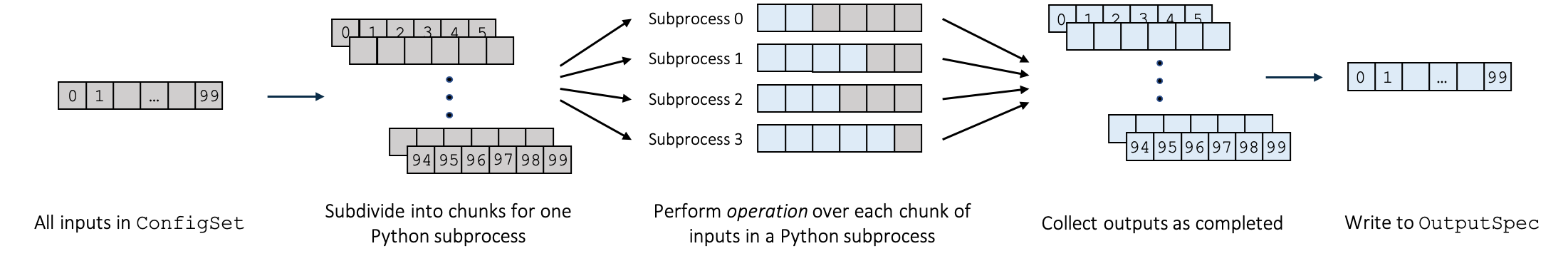
Figure 1: Illustration of the autoparallelization mechanism. Colors indicate the status of each configuration: gray for unprocessed, and blue for a completed operation.

One advantage to storing intermediate steps in files is that they can be used to recover from a partially complete sequence of operations. To facilitate this possibility, the default behavior for wfl operations is to skip over the actual operation if OutputSpec indicates file storage and all the files already exist. To avoid mistaking partially complete operations for successfully completed ones, the low level routines initially write the output to temporary filenames, and only rename them to the intended final names once the operation is complete. Note that this mechanism is very simple, relying only on the existence of files with particular names, so it is not aware of changes in the code. As a result, during development it is necessary for the user to manually delete any output files created by functions that have been modified since the previous run. Also, writing the intermediate results to file storage does lead to a small additional computational cost. For example, the simple workflow example discussed in Section III.6 is about 4% (23 s) slower if all of the OutputSpecs write to an extended xyz file instead of keeping the structures in-memory.

III.2 Simple autoparallelization

Since this interface is designed for operations that can be done independently for each configuration, it is trivial to parallelize, as illustrated in Fig. 1. The implementation has been encapsulated by a Python wrapper defined in wfl.autoparallelize, but a full description of its details are beyond the scope of this article. Using this automatic parallelization is very simple, and can be controlled by a combination of an AutoparaInfo object and an environment variable, both optional. In the simplest case, the Python calling syntax is as shown above, and the only additional requirement for activating the parallelization is to set the environment variable WFL_NUM_PYTHON_SUBPROCESSES="N", where N is the number of Python processes to parallelize over. It is also possible to set this value from Python, by passing an AutoparaInfo object

⬇

from wfl.autoparallelize import AutoparaInfo

autopara_info = AutoparaInfo(num_python_subprocesses=8)

evaluated_configs = generic.calculate(

inputs, outputs, calc=calc,

autopara_info=autopara_info)

The autoparallelize wrapper ensures that all autoparallelized functions take inputs and outputs as their first two arguments, and the autopara_info keyword argument. The sequence of configurations given as inputs are broken up into chunks and passed to a number of Python processes (defined by the environment variable or AutoparaInfo argument) which execute the low-level function implementing the operation. Returned configurations are reassembled according to the original inputs sequence and written to the location indicated by outputs.

One limitation of this design is that all arguments passed to and results returned from the function must be picklable, because Python’s multiprocessing.pool, which we use, depends on the pickle module to communicate with the subprocess running the called function. One important use case, GAP ASE calculator class Potential defined in quippy.potential, does not satisfy this requirement. As a result, the generic.calculate wrapper will also accept a 3-element tuple, instead of an instantiated Calculator object, with the structure

⬇

calc = (quippy.potential.Potential,

[], {"param_filename"="GAP.xml"})

where the first element is the constructor method, the second is a list of positional arguments, and the third is a dictionary of keyword arguments.

III.3 Parallelizing expensive operations over independent queued jobs

In addition to facilitating parallelization over Python subprocesses, the autoparallelize wrapper also makes it easy to break up the work into a set of independent jobs for execution with a queuing system, illustrated in Fig. 2. This capability is especially important for operations where the cost of application to a single configuration is substantial, e.g. single-point DFT evaluations of a potential fitting database. This functionality is provided using the new ExPyRe Python package for Executing Python Remotely. From the point of view of the wfl user, the only additional requirement is to specify information about the remote job in the AutoparaInfo argument, including the computer system where it will run and the resources required. ExPyRe is designed for HPC facilities with a queuing system—PBS, SLURM and SGE are currently supported. The computer where the script using wfl runs (but not necessary the HPC system where the jobs will run) must have a configuration file describing the available systems and resources where the queued jobs can be submitted, as well as the wfl and ExPyRe Python packages. This workflow-running machine can be a login node of the HPC system, or a different computer whose job submission node is accessible via ssh. The HPC system compute nodes must have Python and wfl installed, but no other Python packages are required except what is necessary to carry out the actual desired computation, e.g. quippy or phonopy.

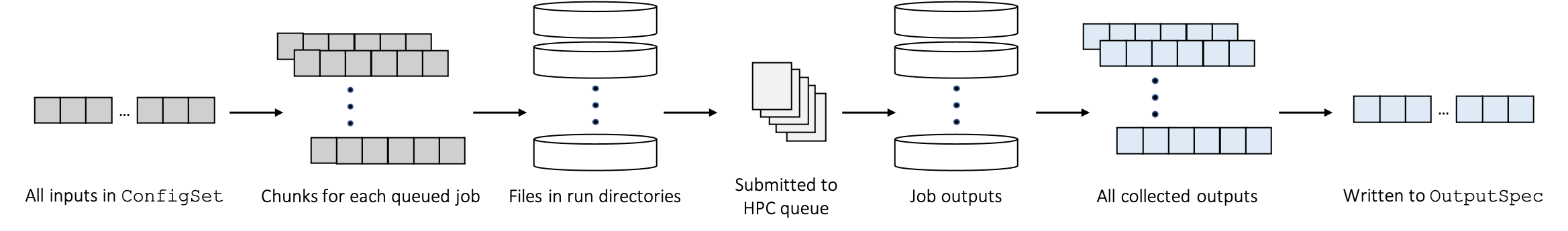
Figure 2: Illustration of autoparallelization mechanism with remote execution (colors as in Fig. 1). Within each queued job further parallelization can be carried out, as described in Section III.2 and Figure 1.

The configuration information is by default stored at "$\sim$/.expyre/config.json", and contains a dict with a systems key with entries such as

⬇

{"systems": {

"local_HPC": {

"host": null,

"scheduler": "sge",

"commands": [

"conda activate myenv"

],

"header": [

"#$ -pe smp {num_cores}"

],

"partitions": {

"standard": {

"num_cores": 16,

"max_time": "168h",

"max_mem": "200GB"

}}}}}

This example describes a system with no remote host (i.e. jobs will be submitted on the machine where the wfl-using script runs), using the SGE queuing system with one optional queued job header line, and a single conda command to run at the start of any job. The system has only one partition type, named “standard”, which has the specified node core count, memory, and time limit. ExPyRe will use this information to create the job script, including the mandatory header lines, which will be submitted for each remote job.

With this configuration in place, breaking up the inputs into groups to be run in a series of queued jobs requires only a small addition to the generic.calculate calling syntax, an optional argument to the AutoparaInfo constructor:

⬇

from wfl.autoparallelize import AutoparaInfo, RemoteInfo

remote_info = RemoteInfo(

sys_name="local_HPC",

job_name="REF_evaluation",

num_inputs_per_queued_job=1,

resources={

"num_nodes": 1,

"max_time": "1h",

"partitions": "standard"},

input_files=["pseudopotentials"])

\parautopara_info = AutoparaInfo(remote_info=remote_info)

The RemoteInfo object specifies the system name from the "$\sim$/.expyre/config.json" file, an arbitrary name for labeling the submitted job, and the number of configurations from the inputs iterable to group for each queued job. In addition, the object specifies the required queuing system resources for each job, one node for one hour on the partition named “standard” (matching the configuration file entry for this system), and finally, the "pseudopotentials" subdirectory will be copied for each remote job by ExPyRe.

The DFT single-point evaluation use case also has other implications for the way wfl manages the calculations. Because ASE does most DFT calculations using third-party software that relies on files for input and output, wfl wraps DFT calculators such as ase.calculators.espresso.Espresso to make them more applicable to its intended use. It runs each instance of the DFT program in a separate subdirectory so multiple side-by-side runs do not overwrite each other, and can automatically select a distinct $\Gamma$-point-only executable for nonperiodic configurations. The calculator that will be passed to generic.calculate is defined by a class inheriting from the underlying ASE calculator, with some additional optional arguments to control the directories and files created during the calculation. Note however, that in general we do not introduce any new functionality (such as DFT convergence checks) in addition to what is provided in the underlying ASE interface and only extend the ASE’s Calculators to not interfere across parallelized instances.

⬇

from wfl.calculators.espresso import Espresso

dft_calc = Espresso(

pseudopotentials={"Si": "Si.UPF"},

pseudo_dir="pseudopotentials",

input_data={

"SYSTEM": {

"ecutwfc": 40,

"input_dft": "LDA"}},

kpts=(2, 3, 4),

conv_thr=0.0001)

All of the arguments used here are standard ase.calculators.espresso.Espresso constructor arguments, without any of our subclass-specific arguments that would modify the default behavior of running in a subdirectory named "./run_QE_$<$RANDOM_STR$>$", and keeping only files required for NOMADDraxl_2019 upload, i.e. "*.pwo".

The call to do the DFT evaluations is simply

⬇

from wfl.calculators import generic

evaluated_configs = generic.calculate(

inputs, outputs, calc=dft_calc,

autopara_info=autopara_info)

This call to generic.calculate will break up the inputs into groups of one configuration each, prepare and submit each job, and wait for them to be finished before assembling the returned configurations and storing them in the location specified by the outputs argument. Except for the need to wait, executing this script with remote execution should be entirely equivalent to running the same sequence of function calls locally. An optional timeout argument to the RemoteInfo constructor specifies the maximum waiting time. If this time is exceeded and an exception is raised, or the user aborts the script before all the jobs are complete, rerunning the wfl script will automatically resume by looking for the previously submitted jobs, gathering their results if they are now complete (or waiting for the rest), and continuing with any further actions in the script. Note that as for the reuse of output files generated by any autoparallelize operation (Sec. III.1), this job caching mechanism is not aware of changes to the code, and the user must manually wipe the staged jobs if the underlying code has been modified.

Given the possibility of many nested types and levels of parallelism, there can be many ways to distribute of the work of each operation among jobs, nodes, and cores. The number of configurations grouped into each job is specified by RemoteInfo.num_inputs_per_queued_job, which divides the number of configurations in the input ConfigSet to determine the number of jobs that are created and submitted to the HPC queue. The number of nodes allocated for each job is set by the RemoteInfo.resources.num_nodes argument. Within each job, the number of operations executed in parallel is given by AutoparaInfo.num_python_subprocesses. Since controlling the full range of possible parallelism in the remote job would add a lot of complexity, we recommend two simpler configurations. One is to use single-node jobs (i.e. num_nodes=1) with multiprocessing.pool-based autoparallelization, where multiple configurations are evaluated in parallel, each using a single core (the default behavior). The other is to use multi-node jobs with MPI-aware operations (e.g. DFT evaluation executables) without autoparallelizing over configurations (i.e. set RemoteInfo.num_inputs_per_queued_job=1 or AutoparaInfo.num_python_subprocesses=1).

III.4 Non-parallelized operations

Some operations that are computationally expensive, but not embarrassingly parallel have also been wrapped in wfl, in particular the actual fitting of MLIPs. For example, fitting a GAP model can be done with

⬇

from wfl.fit.gap.simple import run_gap_fit

run_gap_fit(

fitting_configs=training_configs,

fitting_dict=gap_fit_cli_params,

stdout_file=’gap_fit.out’,

skip_if_present=True,

remote_info=remote_info)

This function is a wrapper of the gap_fit executable which is aware of, but does not abstract away, its interface. The gap_fit_cli_params argument is a dictionary that is converted to the command line parameters for the gap_fit executable. The wrapper can detect if the GAP fit appears to have been completed and skips the task if skip_if_present is set to True, but unlike autoparallelized operations this is implemented manually in the run_gap_fit function. The remote_info argument specifies the queuing system resources required to run this GAP fit, e.g. a large memory node if the fitting database is large, or a remote cluster if using the MPI parallel version of GAP fit.

Since the output of this function is not a set of atomic configurations, it does not return a ConfigSet, but only saves the resulting GAP MLIP to a file. The name of the resulting GAP model file is specified by the standard gap_fit command line argument "gap_file", which should be included in gap_fit_cli_params.

III.5 Daisy-chaining operations

One important aspect of the design of wfl autoparallelized operations for workflow applications is that they return a ConfigSet, so the output of each function can be used as the inputs argument of the next. For example, evaluating the reference energy for a set of configurations and then selecting only the ones with low energy/atom can be done with

⬇

all_atoms = ConfigSet("atoms_init.xyz")

\parfrom wfl.calculators import generic

ref_eval_configs = generic.calculate(

all_atoms,

OutputSpec("atoms_REF_evaluated.xyz"),

property_prefix="REF_",

calc=dft_calc)

\parlow_REF_E_configs = wfl.select.simple.by_bool_function(

ref_eval_configs,

OutputSpec(),

filter_func=lambda a: a.info["REF_energy"]/len(a) < 1.0)

The selection call does not depend on where the output of the first call is stored, since that information is abstracted in the ref_eval_configs object. The simple selection just assumes that Atoms.info["REF_energy"] is defined for the configurations in ref_eval_configs, and the OutputSpec specifies that configurations returned in low_REF_E_configs will be stored only in memory. Any number of steps in the workflow can be chained similarly, and the user can have access, even after the script is complete, to any intermediate result that was specified by a file in an operation’s OutputSpec object.

III.6 Combining elements into a workflow

An example of a more complex multi-step workflow is shown in Fig. 3, and a runnable Jupyter notebook implementing it is available in the SI and online. After importing the needed symbols, the workflow defines the xTB tight-binding method as the reference calculator. It creates isolated atom configurations for each species (not shown in Fig. 3), as well as molecules defined from SMILES strings, and uses those molecules as initial configurations for a finite temperature molecular dynamics run with the xTB calculator. The resulting trajectories are subsampled by computing SOAP descriptors for each configuration and selecting among them with leverage score CUR on the descriptor vectors. A fitting set is used to fit a GAP MLIP, and the predictions of the resulting potential for the fitting set as well as an independent test set are computed. These predictions are then formatted into a printed error table and corresponding parity plots.

It is worth noting, however, that even though extending the new functions with wfl tools may make them more efficient and better integrate with other wfl-wrapped functions (see Section IV), any Python function may be used in a wfl-based workflow. For example, to make use of a new MLIP framework, only a Python function that performs the fitting and an ASE-type Calculator are needed. As a result, it should be straightforward to use other MLIP frameworks or packages with related functionality, such as FitSNAP rohskopf2023fitsnap , FLAME amsler2020flame and BenchML poelking2022benchml , within wfl-based scripts and similarly, wfl’s tools may be useful for doing operations in such frameworks.

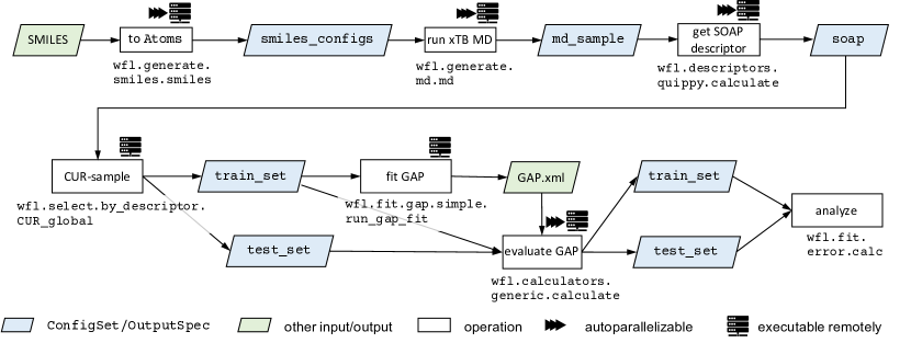
Figure 3: Schematic representation of a more complex daisy-chained workflow. The corresponding Jupyter notebook is available online at https://libatoms.github.io/workflow/examples.daisy_chain_mlip_fitting.html.

IV Wrapping new functions

Section III highlighted key functionality of wfl by a number of simple examples that use functions already written to take advantage of the key functionality. These included atomic structure input and output via the ConfigSet and OutputSpec classes, and controlling automatic parallelisation and executing the functions remotely. However, it is impossible, and we do not aspire, to maintain a full library of wfl-wrapped operations to support all atomistic simulation needs. Instead, we designed wfl so its tools can be easily plugged into any ASE-based script. Below we show examples of how to parallelize a function with wfl.map or wfl.autoparallelize. We also show how to use ExPyRe to remotely execute any function, not limited to those already in wfl or ASE.

IV.1 Parallelizing a new function

IV.1.1 wfl.map

The simplest way to parallelize a new function over multiple Atoms objects, including taking advantage of ConfigSet and OuptutSpec and remote execution, is via wfl.map.map.

As an example, suppose we already have a cap_bonds function which takes a single Atoms object and adds an atom to any dangling bond:

⬇

saturated_at = cap_bonds(dangling_at, cap_with="H")

wfl.map.map takes such a function, with its arguments and keyword arguments, and applies it to each structure in the input ConfigSet and writes to the output OutputSpec.

⬇

import wfl.map

saturated_ats = wfl.map.map(

inputs,

outputs,

map_func=cap_bonds,

kwargs={"cap_with": "H"},

autopara_info=autopara_info)

The parallelized function has to be pickleable and has to take a single Atoms structure as the first positional argument and return an Atoms structure or None. Just like examples in Section III, parallelization and remote execution of wfl.map.map is controlled by an AutoparaInfo object.

This way of parallelizing a function is suitable in cases where starting the paralellized function is computationally inexpensive, because wfl.map calls the function separately for each Atoms object.

IV.1.2 wfl.autoparallelize

In some cases, the initialization step of the parallelized function is significantly more computationally expensive than executing it on a single Atoms object. For example, initializing a GAP Calculator via quippy.potential.Potential in extreme cases can take minutes (because a large parameter file has to be read in and parsed), while evaluation on a single configuration may require only a few seconds. With large numbers of atomic structures to be evaluated, it makes sense to load the potential once per tens or hundreds of structures. Furthermore, the iterable to be parallelized over might not be an atomic structure itself, but an instruction for generating one, as is the case in wfl.generate.smiles and wfl.generate.buildcell submodules. The wfl.autoparallelize wrapper supports both these scenarios.

Functions wrapped in wfl.autoparallelize have to take and return a list of Atoms, hence we define a new function

⬇

def saturate_db(input_atoms, cap_with="H"):

output_atoms = []

for dangling_at in input_atoms:

saturated_at = cap_bonds(dangling_at,

cap_with=cap_with)

output_atoms.append(saturated_at)

return output_atoms

We can autoparallelize this function simply by calling

⬇

from wfl.autoparallelize import autoparallelize

autoparallelize(saturate_db,inputs,outputs,

cap_with="H",autopara_info=autopara_info)

Or define a new, parallelized version of the function:

⬇

def autopara_saturate_db(*args, **kwargs):

default_ap_info={"num_inputs_per_python_subprocess":100}

return wfl.autoparallelize.autoparallelize(

saturate_db, *args,

default_autopara_info=default_ap_info,

**kwargs)

Here, before returning the wrapped function, we additionally set the default value for num_inputs_per_python_subprocess. The new autopara_saturate_db can then be used as in the examples in Sections III .To work with autoparallelize, the operation must take in an iterable and return a list (or nested lists) of Atoms objects or None. In most cases, iterable corresponds to a list of input Atoms objects, but can in principle be anything, for example a list of SMILES strings (e.g. SMILES string "CCO" corresponds to ethanol) used to generate Atoms structures, as in wfl.generate.smiles.

The signature of the parallelized autopara_saturate_db is modified from that of saturate_db. The iterable is replaced by inputs (a ConfigSet) and outputs (an OutputSpec) and it accepts an AutoparaInfo object which controls parallelization.

⬇

capped_structures = autopara_saturate_db(

inputs,

outputs,

cap_with="H",

autopara_info=autopara_info)

IV.2 Execute Python Remotely

Running remote jobs in wfl is done using ExPyRe, which wraps individual Python functions, executes them in remote jobs, and returns their results. It is inspired by MyQueuemortensen2020myqueue , but designed with somewhat different limitations and capabilities motivated by our functionality and computational resource use cases. The autoparallelizing wrapper ensures that all autoparallelized functions interface with ExPyRe. In addition, some non-autoparallelize-able yet computationally expensive tasks, such as fitting GAP and ACE interatomic potentials, are an important part of atomistic workflows and are also interfaced with ExPyRe directly. The key steps performed by ExPyRe are illustrated in Figure 4.

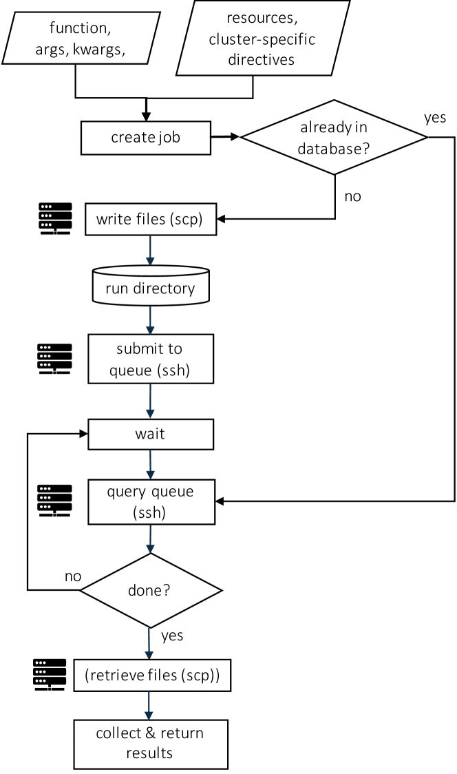
Figure 4: Illustration of steps performed by ExPyRe when executing functions remotely. Pictogram indicates actions that may be executed on a remote cluster.

To execute any function with ExPyRe (let us continue with the cap_bonds example), a couple of extra Python objects need to be defined, as illustrated in the following script. Note that RemoteInfo is not applicable here, because it combines wfl-specific options with ExPyRe arguments.

⬇

xpr = expyre.func.ExPyRe(’test_task’,

function=cap_bonds,

args=[dangling_at],

kwargs={’cap_with’: "H"})

\parresources = {’max_time’: ’1h’,

’num_nodes’: 1,

’partitions’: ’regular’}

\parxpr.start(resources=resources, system_name=’remote’)

saturated_at, stdout, stderr = xpr.get_results()

First, an ExPyRe instance is created in which we specify the function that will be executed remotely, as well as its positional and keyword arguments. Together with xpr.start these steps write input files for the job, write a queue-specific job submission script and submit the job. In this step, job-specific resources (required time, number of nodes or cores, queue or partition) are also provided and used to specify the correct resources in the job submission script. As in the examples from Section III, the cluster-specific configuration file must be present.

At the xpr.get_results stage, ExPyRe periodically queries the queueing system for status of the job while waiting for its completion. At this point, the Python script may be killed and restarted to continue without re-submitting the jobs. The jobs and their status are tracked in a file-based sqlite database which can be queried via a convenience command line interface, xpr.

File copying and job queue querying is executed via a passwordless ssh, for example by using public/private keys, kerberos authentication, or by multiplexing SSH connections to reuse a previously established password- or multifactor-authenticated connection.

There are several files associated with the remote execution process used for communication between the local Python script and remote queued job. These files include the pickled input function and its output, the job submission script and outputs as well as files used by ExPyRe to track and report on job’s progress. Normally, the user does not need to be concerned with these files, but it is useful to be aware of the behind-the-scenes working of ExPyRe for occasional debugging, since we expect these tools to be used in developing a wide variety of projects and scripts. These auxiliary files can also be deleted using the command line interface, xpr.

One consequence of the pickle-based remote execution mechanism is that the function to be executed remotely (e.g. cap_bonds or saturate_db) must be imported into the script that wraps it with wfl.autoparallelize or wfl.map (or any other way that results into passing it to ExPyRe). This is because pickling a function does not save the function’s content, only its full name including package information, which is used to import it when the pickled data is unpickled by the remotely executed job. The solution is to define the original function either in a Python package that is installed on both the local and remote machines, or in a separate file that is included in RemoteInfo.input_files and therefore copied over to the run directory on the remote machine.

V Summary

In summary, we introduced the Python-based workflow management package wfl and the remote execution package ExPyRe, which are designed to support the versatile requirements of computations commonly used in atomistic simulation and MLIP fitting processes. wfl is designed as a lightweight platform to provide efficient parallelization capabilities for various numbers and sizes of embarrassingly parallel tasks with computational demands that range from milliseconds on a single core up to hours on several nodes. These parallel tasks can optionally be executed on a HPC queueing system via the general-purpose Python remote execution framework ExPyRe. The two packages provide a few low-level functions - input and output abstraction classes, an autoparallelization wrapper, and a remote execution functionality - to wrap any operation, as well as wrapped versions of a number of commonly used operations. Using this developer-oriented functionality, high level user-friendly functions can be easily produced by combining these and other operations to construct reproducible calculation workflows. Some common instances of such high level functions are already present in the wfl package, and we provide examples of how to make use of wfl’s functionality for custom functions and workflows.

In contrast to other material simulation workflow packages that focus on ab initio data generation and provenance, wfl is designed to provide low-level support for efficiently parallelizing and integrating a wide variety of operations for atomistic simulations. One distinctive feature is its focus on using human-readable formats and storage, and on minimizing the need for system infrastructure such as remotely accessible database servers. Another is the use of a small number of python classes to abstract atomic configuration storage and to support efficient execution of embarrassingly parallel operations, whether they are computationally demanding individually or only in the aggregate. The package is developer-oriented, and intended for use in research areas where the development of the particular sequence of computational operations to be done is a complex and significant part of the overall research task.

We believe that wfl will fill an important niche in the atomistic simulation communities that develop new computational procedures with tools that implement them using Python libraries such as ASE. While the basic functionality of ASE has already revolutionized the way atomistic simulation software is being developed, wfl will extend its range of applicability further by abstracting the details of atomic configuration, and providing easy to use automatic parallelization and remote execution. Its design principles of lightweight, modularity, and human-inspectability should make it easy to incorporate into existing ASE-based scripts. We hope that it will prove useful for a wide range of atomistic simulations.

VI Code Availability

The wfl and ExPyRe codes are available in the GitHub respositories, https://github.com/libAtoms/workflow and https://github.com/libAtoms/ExPyRe. Additionally, documentation, including examples and API, are accessable at https://libatoms.github.io/workflow and https://libatoms.github.io/ExPyRe.

VII Data Availability

Data sharing is not applicable to this article as no new data were created or analyzed in this study.

VIII Acknowledgements

We are grateful for computational support from the UK national high-performance computing service, ARCHER2, for which access was obtained via the UKCP consortium and funded by EPSRC grant reference EP/P022596/1. N.B. acknowledges support by the U. S. Naval Research Laboratory’s 6.1 fundamental research base program, and computer time support from the DOD HPCMPO at the AFRL, ERDC, and ARL MSRCs. E.G. acknowledges support from the EPSRC Centre for Doctoral Training in Automated Chemical Synthesis Enabled by Digital Molecular Technologies with grant reference EP/S024220/1. T.K.S. acknowledges support from the European Union’s Horizon 2020 Research and Innovation Program under Grant Agreement No. 957189 (BIG-MAP project). S.W., H.H. and K.R. gratefully acknowledge the Max Planck Computing and Data Facility (MPCDF) for providing computing time.

For their contributions to the code development the authors want to acknowledge Nikhil Bapat, Lars Schaaf, Nicolas Bergmann, Xu Han and Felix Riccius. We also thank Olga Vinogradova and Felix Riccius for creating the logo.

For the purpose of open access, the authors have applied a Creative Commons Attribution (CC BY) licence to any Author Accepted Manuscript version arising from this submission.

IX Author Contribution

G.C., N.B. and T.K.S. jointly conceived the project. N.B., E.G., S.W. and T.K.S. designed, implemented and tested the software. N.B., G.C., H.H.H. and K.R. supervised the project, N.B., G.C. and K.R. acquired funding. E.G., N.B. and H.H.H. prepared the original draft of the paper. All authors reviewed and edited the manuscript.

X Competing interests

Authors declare no competing interests.

References

- [1] Maximilian Amsler, Samare Rostami, Hossein Tahmasbi, Ehsan Rahmatizad Khajehpasha, Somayeh Faraji, Robabe Rasoulkhani, and S Alireza Ghasemi. Flame: a library of atomistic modeling environments. Computer Physics Communications, 256:107415, 2020.
- [2] Albert P Bartók, Mike C Payne, Risi Kondor, and Gábor Csányi. Gaussian approximation potentials: The accuracy of quantum mechanics, without the electrons. Physical review letters, 104(13):136403, 2010.
- [3] Kamal Choudhary, Kevin F Garrity, Andrew CE Reid, Brian DeCost, Adam J Biacchi, Angela R Hight Walker, Zachary Trautt, Jason Hattrick-Simpers, A Gilad Kusne, Andrea Centrone, et al. The joint automated repository for various integrated simulations (jarvis) for data-driven materials design. npj computational materials, 6(1):173, 2020.
- [4] Stefano Curtarolo, Wahyu Setyawan, Gus LW Hart, Michal Jahnatek, Roman V Chepulskii, Richard H Taylor, Shidong Wang, Junkai Xue, Kesong Yang, Ohad Levy, et al. Aflow: An automatic framework for high-throughput materials discovery. Computational Materials Science, 58:218–226, 2012.
- [5] Daniele Dragoni, Thomas D Daff, Gábor Csányi, and Nicola Marzari. Achieving dft accuracy with a machine-learning interatomic potential: Thermomechanics and defects in bcc ferromagnetic iron. Physical Review Materials, 2(1):013808, 2018.
- [6] Ralf Drautz. Atomic cluster expansion for accurate and transferable interatomic potentials. Physical Review B, 99(1):014104, 2019.
- [7] Claudia Draxl and Matthias Scheffler. The nomad laboratory: from data sharing to artificial intelligence. Journal of Physics: Materials, 2(3):036001, 2019.
- [8] Genevieve Dusson, Markus Bachmayr, Gábor Csányi, Ralf Drautz, Simon Etter, Cas van der Oord, and Christoph Ortner. Atomic cluster expansion: Completeness, efficiency and stability. Journal of Computational Physics, 454:110946, 2022.
- [9] Marco Esters, Corey Oses, Simon Divilov, Hagen Eckert, Rico Friedrich, David Hicks, Michael J Mehl, Frisco Rose, Andriy Smolyanyuk, Arrigo Calzolari, et al. aflow. org: A web ecosystem of databases, software and tools. Computational Materials Science, 216:111808, 2023.
- [10] Morten Gjerding, Thorbjørn Skovhus, Asbjørn Rasmussen, Fabian Bertoldo, Ask Hjorth Larsen, Jens Jørgen Mortensen, and Kristian Sommer Thygesen. Atomic simulation recipes: A python framework and library for automated workflows. Computational Materials Science, 199:110731, 2021.
- [11] Anubhav Jain, Shyue Ping Ong, Wei Chen, Bharat Medasani, Xiaohui Qu, Michael Kocher, Miriam Brafman, Guido Petretto, Gian-Marco Rignanese, Geoffroy Hautier, et al. Fireworks: a dynamic workflow system designed for high-throughput applications. Concurrency and Computation: Practice and Experience, 27(17):5037–5059, 2015.
- [12] Anubhav Jain, Shyue Ping Ong, Geoffroy Hautier, Wei Chen, William Davidson Richards, Stephen Dacek, Shreyas Cholia, Dan Gunter, David Skinner, Gerbrand Ceder, et al. Commentary: The materials project: A materials genome approach to accelerating materials innovation. APL materials, 1(1):011002, 2013.
- [13] Jan Janssen, Sudarsan Surendralal, Yury Lysogorskiy, Mira Todorova, Tilmann Hickel, Ralf Drautz, and Jörg Neugebauer. pyiron: An integrated development environment for computational materials science. Computational Materials Science, 163:24–36, 2019.
- [14] Scott Kirklin, James E Saal, Bryce Meredig, Alex Thompson, Jeff W Doak, Muratahan Aykol, Stephan Rühl, and Chris Wolverton. The open quantum materials database (oqmd): assessing the accuracy of dft formation energies. npj Computational Materials, 1(1):1–15, 2015.
- [15] Jan Kloppenburg, Livia B Pártay, Hannes Jónsson, and Miguel A Caro. A general-purpose machine learning pt interatomic potential for an accurate description of bulk, surfaces, and nanoparticles. The Journal of chemical physics, 158(13), 2023.
- [16] Greg Landrum. Rdkit: Open-source cheminformatics. https://www.rdkit.org.
- [17] Ask Hjorth Larsen, Jens Jørgen Mortensen, Jakob Blomqvist, Ivano E Castelli, Rune Christensen, Marcin Dułak, Jesper Friis, Michael N Groves, Bjørk Hammer, Cory Hargus, et al. The atomic simulation environment—a python library for working with atoms. Journal of Physics: Condensed Matter, 29(27):273002, 2017.
- [18] Daniel Marchand, Abhinav Jain, Albert Glensk, and WA Curtin. Machine learning for metallurgy i. a neural-network potential for al-cu. Physical review materials, 4(10):103601, 2020.
- [19] Kiran Mathew, Joseph H Montoya, Alireza Faghaninia, Shyam Dwarakanath, Muratahan Aykol, Hanmei Tang, Iek-heng Chu, Tess Smidt, Brandon Bocklund, Matthew Horton, et al. Atomate: A high-level interface to generate, execute, and analyze computational materials science workflows. Computational Materials Science, 139:140–152, 2017.
- [20] Hossein Mirhosseini, Hossein Tahmasbi, Sai Ram Kuchana, S Alireza Ghasemi, and Thomas D Kühne. An automated approach for developing neural network interatomic potentials with flame. Computational Materials Science, 197:110567, 2021.
- [21] J Harry Moore, Matthias R Bauer, Jeff Guo, Atanas Patronov, Ola Engkvist, and Christian Margreitter. Icolos: A workflow manager for structure based post-processing of de novo generated small molecules. 2022.
- [22] Jens Jørgen Mortensen, Morten Gjerding, and Kristian Sommer Thygesen. Myqueue: Task and workflow scheduling system. Journal of Open Source Software, 5(45):1844, 2020.
- [23] https://libatoms.github.io/workflow/examples.daisy_chain_mlip_fitting.html.
- [24] The comparison is made on the example workflow script, appropriate steps parallelized over 16 cores with no remote execution, and 10 times more starting SMILES strings and structures in the training and testing sets.
- [25] Shyue Ping Ong, William Davidson Richards, Anubhav Jain, Geoffroy Hautier, Michael Kocher, Shreyas Cholia, Dan Gunter, Vincent L Chevrier, Kristin A Persson, and Gerbrand Ceder. Python materials genomics (pymatgen): A robust, open-source python library for materials analysis. Computational Materials Science, 68:314–319, 2013.
- [26] Chris J Pickard and R J Needs. Ab initio random structure searching. Journal of Physics: Condensed Matter, 23(5):053201, jan 2011.
- [27] Giovanni Pizzi, Andrea Cepellotti, Riccardo Sabatini, Nicola Marzari, and Boris Kozinsky. Aiida: automated interactive infrastructure and database for computational science. Computational Materials Science, 111:218–230, 2016.
- [28] Carl Poelking, Felix A Faber, and Bingqing Cheng. Benchml: an extensible pipelining framework for benchmarking representations of materials and molecules at scale. Machine Learning: Science and Technology, 3(4):040501, 2022.
- [29] Marvin Poul, Liam Huber, Erik Bitzek, and Jörg Neugebauer. Systematic atomic structure datasets for machine learning potentials: Application to defects in magnesium. Physical Review B, 107(10):104103, 2023.
- [30] A Rohskopf, C Sievers, N Lubbers, Ma Cusentino, J Goff, J Janssen, M McCarthy, D Montes Oca de Zapiain, S Nikolov, K Sargsyan, et al. Fitsnap: Atomistic machine learning with lammps. Journal of Open Source Software, 8(84):5118, 2023.
- [31] James E Saal, Scott Kirklin, Muratahan Aykol, Bryce Meredig, and Christopher Wolverton. Materials design and discovery with high-throughput density functional theory: the open quantum materials database (oqmd). Jom, 65:1501–1509, 2013.