∎
∗Corresponding author: shenglanyuan@hust.edu.cn
Computing large deviation prefactors of stochastic dynamical systems based on machine learning
Abstract
In this paper, we present large deviation theory that characterizes the exponential estimate for rare events of stochastic dynamical systems in the limit of weak noise. We aim to consider next-to-leading-order approximation for more accurate calculation of mean exit time via computing large deviation prefactors with the research efforts of machine learning. More specifically, we design a neural network framework to compute quasipotential, most probable paths and prefactors based on the orthogonal decomposition of vector field. We corroborate the higher effectiveness and accuracy of our algorithm with a practical example. Numerical experiments demonstrate its powerful function in exploring internal mechanism of rare events triggered by weak random fluctuations.
Keywords:
Machine learning large deviation prefactors stochastic dynamical systems rare eventspacs:
PACS 05.10.-a PACS 05.10.Gg PACS 05.40.-a PACS 02.50.-r1 Introduction
The phenomena of rare events exit from the domain of attraction of a stable state induced by noise have been attracting increasing attention in recent years, ranging from physics MX ; ZY ; SB , chemistry DM , biology YLZ ; YZD , to engineering ZW ; ZJ . Even for weak noise, the rare events will occur almost surely, if the observations are performed on a sufficiently long time scale. The expected time required for observing this phenomena to occur, i.e., mean exit time, typically grows exponentially as the intensity of the random perturbations tends to zero.
Freidlin and Wentzell established large deviation theory to understand and analyze such dynamics in the limit of weak noise FW . They proposed a vital concept of action functional to estimate the probability of the stochastic trajectory passing through the neighborhood of a given curve. The global minimum of the action functional is called quasipotential which exponentially dominates the magnitude of stationary probability distribution and mean exit time. However, the exponential estimate of large deviation theory is too rough since it smears all the possible polynomial coefficients prior to the exponent. Thus a reasonable estimation or an symptotic approximation of the large deviation prefactor is required, in order to gain a more accurate mean exit time.
Traditionally, shooting method is a feasible technique to compute the prefactor of mean exit time. Its idea is to derive a group of ordinary differential equations via WKB approximation and method of characteristics NK ; MST ; MS ; R ; MS97 ; BR22 ; BM . Then the WKB prefactor and further the prefactor of mean exit time can be computed by integrating this group of equations. However, this method requires searching for the most probable path connecting the fixed point to the point with minimal quasipotential on the boundary, which is not an easy task, especially for high-dimensional systems.
We have witnessed in recent years a rapid development of data science and computer technology EW . In view of the powerful nonlinear representation ability of machine learning, many researchers applied it to the investigation of stochastic dynamics. For example, machine learning methods can be used to discover stochastic dynamical systems from sample path data via nonlocal Kramers-Moyal formulas LD ; LD22 , physics-informed neural networks KK ; RV , and variational inference O . They are also used to solve physical quantities of stochastic dynamical systems via computing most probable path LDL ; W , quasipotential LXD ; LLR ; LYX , and probability density XZL . These experimental results show the potential applications of the combination between machine learning and stochastic dynamics.
In this research, our goal is to develop machine learning method to compute the large deviation prefactors in the highly complex nonlinear nondeterministic systems. We generate a specific algorithm for training multilayer artificial networks and perform complex computations through a learning process. The information-processing architecture is composed of neurons and synaptic weights converting electrical signals. It provides a means of minimizing the error function, and even suggests a possible treatment of mean exit time.
The structure of this article is arranged as follows. In Section 2, we simply introduce the large deviation theory and the quasipotential concept. In Section 3, we describe the results for the prefactors of mean exit time in the cases of non-characteristic and characteristic boundaries. In Section 4,, we design the machine learning method for computing the prefactors. Numerical experiments are performed in Section 5 to verify the effectiveness and accuracy of the algorithm. Section 6 presents the conclusion and innovations.
2 Large deviation theory
We consider here -dimensional stochastic differential equation (SDE) modeled by
| (1) |
where is the vector field, denotes Brownian motion, and indicates a small noise intensity. Even though noise is weak, rare events, such as exit or transition problems induced by noise, will occur with probability one in sufficiently long time scale. Freidlin and Wentzell proposed large deviation theory to analyze and compute these phenomena FW .
For the solution of system (1), the Freidlin-Wentzell action functional is in the form of
with the corresponding Lagrangian . The definition of quasipotential is given by
| (2) |
Note that the quasipotential of the fixed point equals zero, i.e., . The quasipotential actually illustrates the possibility of the system appearing around .
The associated Fokker-Planck equation of SDE (1) is formulated as
where is the probability density. The stationary probability density satisfies
| (3) |
Assume that the stationary distribution is approached by the WKB approximation
| (4) |
where stands for the WKB prefactor. Substituting the WKB approximation (4) into the stationary Fokker-Planck equation (3) yields Hamilton-Jacobi equation
| (5) |
Introducing the canonical momentum
the Hamiltonian is actually the Legendre transformation of the Lagrangian.
According to Eq. (5), it follows that
which thus infers the orthogonality relation
| (6) |
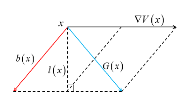
Define . It is immediately obvious that , which is concerned with an orthogonal decomposition of the vector field as seen from Fig. 1. The vector field dominates the direction of the most probable path.
It should be pointed out that the WKB prefactor is determined by
where represents the most probable exit path, denotes the divergence, and is the point at which attains its global minimum, i.e., the stable fixed point (BR16, , Section 3).
3 Mean exit time
Given an open subset domain , the first exit time is defined by the stopping time
Estimating the mean first exit time starting from the stable fixed point requires minimizing the action functional over all exit times in terms of the Freidlin-Wentzell large deviation theory. Performing this minimization over paths from the point to the basin boundary yields the Arrhenius law
Therefore,
| (7) |
We compute the above prefactor in two different cases.
Case A. non-characteristic boundary (BR22, , Section 4.1).
Assume that the domain is an open, smooth and connected subset of satisfying the following conditions, where indicates the exterior normal vector at .
- (A1)
-
The deterministic system possesses a unique fixed point in , which attracts all the trajectories started from , and for all .
- (A2)
-
The function is -continuous in ; for any , the most probable path goes to as ; and for all .
- (A3)
-
The minimum of over is reached at a single point , at which
and the quadratic form has positive eigenvalues on the hyperplane .
If for all , the boundary is said to be non-characteristic. This condition ensures that the dynamical trajectories started from the closure will remain and that the vector field is transverse with the boundary. By Assumption (A1), we derive the integral formula BR22 ; BR16
for the exit rate . Using the second-order expansion of in the neighborhood of in this formula, we obtain the equivalent relation of the prefactor
| (8) | ||||
where we use
Case B. characteristic boundary (BR22, , Section 4.2).
The basin domain is characteristic in the sense that for all . We consider the metastable case that the deterministic system possesses two stable fixed points and , whose basins of attractions are separated by a smooth hypersurface . We consider the exit events from the basin of attraction of and formulate the following set of assumptions.
- (B1)
-
All the trajectories of the deterministic system started on remain in and converge to a single fixed point ; in addition, the Jacobi matrix possesses eigenvalues with negative real part and a single positive eigenvalue .
- (B2)
-
Indicating the quasipotential with respect to as , there exists a unique (up to time shift) trajectory such that
- (B3)
-
is smooth in the neighborhood of , and the vector field defined by satisfies the orthogonality relation.
In this context, the quasipotential achieves its minimum on at the point . Moreover, the path is called the most probable exit path and it satisfies
For any , it coincides with the path connecting with , in the sense that
In order to describe the prefactor in this case, we formulate the following supplementary assumption.
- (B4)
-
The matrix exists and has positive eigenvalues and 1 negative eigenvalue.
Based on these four assumptions, an asymptotic formula for estimating the expected time taken by the process to exit was obtained in (BR16, , Eq. (1.10)), i.e.,
| (9) |
4 Method
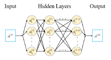
To compute the large deviation prefactors defined in Section 3, we are devoted to developing a machine learning method inspired by Ref. LLR . The critical idea is to design the graphic of the feedforward multilayer neural network shown in Fig. 2 to realize the orthogonal decomposition of the vector field. The neural network is made up of three basic components: an input vector , a set of hidden layers with some synapses connecting neurons, and an output layer . For , there are neurons in the -th hidden layer. The subscript denotes the training parameters in the neural network.
Note that the quasipotential is similar to a quadratic function around the stable fixed point . In order to guarantee that the quasipotential and its gradient are all unbounded, we define the quasipotential . To train the neural network, we construct the loss function , where and are weighted parameters harmonizing the proportion of several parts of loss function.
In order to design the loss function, we randomly select points in the domain of interest in -dimensional Euclidean space . Since the vector field can be decomposed as , the first part of the loss function can be set as
Due to the orthogonal condition , we specify the second part of the loss function as
where we add a sufficiently small parameter , avoiding the divergence of in the case of . The quasipotential is zero at the fixed point, so we fix .
To examine the accuracy of the algorithm, we define the approximation error functions for the quasipotential and the rotational component of vector field by
where and are the prediction results of the neural network, and and mean the true results. According to the expression of for the mean first exit time in Section 3 , the computation of the prefactor essentially depends on the results of the most probable path and the rotational component . After training the neural network, the most probable path satisfies
For numerical convenience, we transform the parameter of this equation into the arc length of the most probable path. Then
where the last equality comes from as in Fig. 1. Therefore, the most probable path satisfies
We can obtain the most probable path from the inverse time integration of the above equation starting from the endpoint until reaching the neighborhood of the fixed point.
With regard to Case A, we choose the point at which the quasipotential reaches its minimum value on the boundary . We calculate in virtue of the neural network results of . Then the integral in can be transformed into
The calculation of the WKB prefactor is already included in the calculation of for Case A. It will no longer be considered separately.
In Case B, we take as the saddle point . For the sake of efficient numerical implementation, our actual operation is to take with the help of a small parameter , where is the unstable direction of . For a small parameter , the inverse time integration terminates when it enters into the -neighborhood of the fixed point . For Case B, we rewrite the integral in into
5 Numerical experiments
To verify the effectiveness and accuracy of the algorithm, we investigate an example with an explicit quasipotential
where and . Define the vector field with
where . It follows from
that . When and ,
| (10) |
If , then we know that there are three fixed points and . To classify those fixed points, we take into account the Jacobian matrix
The Jacobian matrix at is given by
The characteristic equation is , which has complex roots
Thus the two fixed points are asymptotically stable. Using the Jacobian matrix
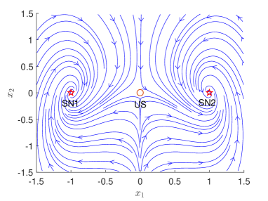
the eigenvalues for are and . Since one eigenvalue is positive and the other is negative, the origin is an unstable saddle point. We sketch a phase portrait for the deterministic system in Fig. 3. The eigenvector for is . The stable manifold is the -axis, which forms the boundary of the left and right basins of attraction. Thanks to the symmetry of the image, we need only consider the exit problem starting from the left side.
The selection of superparameters in algorithm consists of 6 hidden layers with 20 neurons per layer. We choose the Adam optimizer with the learning rate 0.002. The nonlinear activation function for hidden layer is the hyperbolic tangent function . The activation function for output is identity function. The number of training epochs is 100000. We fix , , , and . We randomly select points on the region . After completing the training process, we calculate the approximation errors and with the results shown in Table 1. In the beginning, the errors and gradually decrease as the amount of data increases from to . However, it can be observed that the change is not significant for . At this point, the accuracy of the algorithm is limited by other parameters.
| 100 | 1000 | 10000 | 100000 | |
|---|---|---|---|---|
| 0.3122% | 0.1392% | 0.1267% | 0.0681% | |
| 1.3692% | 0.2127% | 0.0738% | 0.0965% |
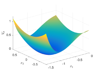
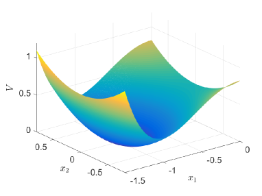
Comparing the numerical results of learned and true quasipotential displayed in Fig. 4 for , it can be seen that the two pictures are consistent with each other.
When , we compute the prefactors for Case A and Case B.
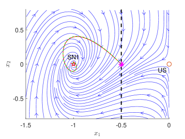
Case A. non-characteristic boundary.
As depicted in Fig. 5, we choose the dashed black line as the non-characteristic boundary for the basin of attraction of SN1. The pink star denotes the exit point, which represents the minimum of the quasipotential on the boundary. By utilizing the results of neural network and true system starting from , we simulate the most probable paths marked as red and dashed green curves, respectively. As indicated in Fig. 5, the two curves match very well.
Define , which satisfies the algebraic Riccati equation
where the matrix
Then we have
Owing to the calculation results of , we can get . The true values of can lead to . The approximate values of are very close in two different situations.
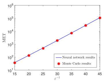
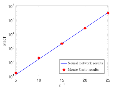
Substituting the prefactor and the quasipotential into the expression of mean exit time , we plot the compared graph between mean exit times via machine learning and Monte Carlo simulation in Fig. 6. The red asterisk denotes the results of Monte Carlo simulation, which is completely consistent with the learning results and has very high accuracy.
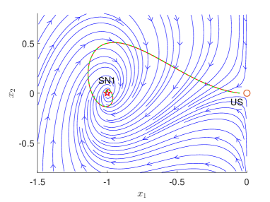
Case B. characteristic boundary.
We treat -axis, i.e., the stable manifold of US, as the boundary of the left and right basins of attraction. On the grounds of neural network, we acquire the most probable path by the dashed green curve that coincides with the red curve of the true system, as shown in Fig. 7.
Define , which satisfies the algebraic Riccati equation
where the matrix
Then we have
We evaluate by the use of the calculation result of , and obtain on the basis of the calculation result of . Putting and into the mean exit time , the comparison chart between the neural network and Monte Carlo results is presented in Fig. 8. It is worth notice that the training result of neural network is highly consistent with the experimental result of Monte Carlo.
6 Conclusion and future perspective
In this work, we developed a machine learning method to establish the large deviation prefactors of stochastic dynamical systems. In particular, we first introduced large deviation theory and the results of prefactors of mean exit time for non-characteristic and characteristic boundaries. Then we provided a new machine learning method to compute the prefactors based on the orthogonal decomposition of the vector field. The successful application of the algorithm to a toy model illustrated its effectiveness of tackling mean exit time accurately.
Our neural networks and algorithm can be effectively extended to and sophisticated high-dimensional circumstances with computational complexity. They can also be generalized to deal with other quantities of rare events such as stationary probability distribution and escape probability. More importantly, our innovative approach may bring forth new ideas for improving the performance of searching for the most probable path by machine learning or data mining.
Acknowledgement
This research was supported by Natural Science Foundation of Jiangsu Province (grant BK20220917) and National Natural Science Foundation of China (grant 12001213).
Data Availability Statement
The data that support the findings of this study are openly available in GitHub
https://github.com/liyangnuaa/Computing-large-deviation-prefactors.
References
- (1) Ma J, Xu Y, Li Y, Tian R, Ma S and Kurths J 2021 Appl. Math. Mech. 42 65-84
- (2) Zheng Y, Yang F, Duan J, Sun X, Fu L and Kurths J 2020 Chaos 30 013132
- (3) Scheffer M, Bascompte J, Brock W A, Brovkin V, Carpenter S R, Dakos V, Held H, Van Nes E H, Rietkerk M and Sugihara G 2009 Nature 461 53-59
- (4) Dykman M I, Mori E, Ross J and Hunt P 1994 J. Chem. Phys. 100 5735-5750
- (5) Yuan S, Li Y and Zeng Z 2022 Math. Model. Nat. Pheno. 17 34
- (6) Yuan S, Zeng Z and Duan J 2021 J. Stat. Mech. Theory E 2021 033204
- (7) Zhu W and Wu Y 2003 Nonlinear Dynam. 32 291-305
- (8) Zhang Y, Jin Y, Xu P and Xiao S 2020 Nonlinear Dynam. 99 879-897
- (9) Freidlin M I and Wentzell A D 2012 Random Perturbations of Dynamical Systems (Berlin: Springer)
- (10) Naeh T, Klosek M, Matkowsky B and Schuss Z 1990 SIAM J. Appl. Math. 50 595-627
- (11) Matkowsky B, Schuss Z and Tier C 1983 SIAM J. Appl. Math. 43 673-695
- (12) Matkowsky B and Schuss Z 1982 SIAM J. Appl. Math. 42 822-834
- (13) Roy R V 1997 Int. J. Nonlin. Mech. 32 173-186
- (14) Maier R S and Stein D L 1997 SIAM J. Appl. Math. 57 752-790
- (15) Bouchet F and Reygner J 2022 J. Stat. Phys. 189 21
- (16) Beri S, Mannella R, Luchinsky D G, Silchenko A and McClintock P V 2005 Phys. Rev. E 72 036131
- (17) E W 2017 Commun. Math. Stat. 5 1-11
- (18) Li Y and Duan J 2021 Physica D 417 132830
- (19) Li Y and Duan J 2022 J. Stat. Phys. 186 30
- (20) Karniadakis G E, Kevrekidis I G, Lu L, Perdikaris P, Wang S and Yang L 2021 Nat. Rev. Phys. 3 422-440
- (21) Rotskoff G and Vanden-Eijnden E 2018 NIPS 31 7146-7155
- (22) Opper M 2019 Annalen der Physik 531 1800233
- (23) Li Y, Duan J and Liu X 2021 Phys. Rev. E 103 012124
- (24) Wei W, Gao T, Chen X and Duan J 2022 Chaos 32 051102
- (25) Li Y, Xu S, Duan J, Liu X and Chu Y 2022 Nonlinear Dynam. 109 1877-1886
- (26) Lin B, Li Q and Ren W 2021 PMLR 145 652-670
- (27) Li Y, Yuan S and Xu S 2023 arXiv:2209.13098
- (28) Xu Y, Zhang H, Li Y, Zhou K, Liu Q and Kurths J 2020 Chaos 30 013133
- (29) Bouchet F and Reygner J 2016 Ann. Henri Poincaré 17 12