Fermionic condensate and the vacuum energy-momentum tensor for planar fermions in homogeneous electric and magnetic fields

Abstract

We consider a massive fermionic quantum field localized on a plane in external constant and homogeneous electric and magnetic fields. The magnetic field is perpendicular to the plane and the electric field is parallel. The complete set of solutions to the Dirac equation is presented. As important physical characteristics of the vacuum state, the fermion condensate and the expectation value of the energy-momentum tensor are investigated. The renormalization is performed using the Hurwitz function. The results are compared with those previously studied in the case of zero electric field. We discuss the behavior of the vacuum expectation values in different regions for the values of the problem parameters. Applications of the results include the electronic subsystem of graphene sheet described by the Dirac model in the long-wavelength approximation.

Keywords: planar fermions, fermion condensate, magnetic catalysis, ground state energy

1 Introduction

The planar fermions appear in describing the properties of a number of condensed matter systems, such as graphene-type materials, topological insulators, etc. Related (2+1)-dimensional quantum field theories also serve as simplified models in elementary particle physics. Among the interesting directions of the corresponding investigations is the study of the behavior of planar fermions in external classical fields. The latter may generate a number of interesting physical effects. In condensed matter systems, described by the effective theory, the ground state corresponds to the vacuum state in the related quantum field theory. The properties of the zero-point fluctuations of the fields in the vacuum state depend on the external fields and therefore the physical characteristics of that state also will depend on them. For fermionic fields, among the important local characteristics are the fermionic condensate and the vacuum average of the energy-momentum tensor. In particular, the fermion condensate is the order parameter describing the phase transitions. In the present paper, we consider a massive fermionic quantum field localized on a plane in external constant and homogeneous electric and magnetic fields.

The quantization of fields requires the knowledge of a complete set of the mode functions being the solutions of the field equation. The solutions of the Dirac equation in external electromagnetic fields have been considered in different cases: (a) Coulomb potential, (b) constant magnetic field, (c) constant electric field, (d) plane wave field, (e) plane wave field with constant magnetic field along the direction of propagation, (f) four cases in which electromagnetic potentials are assumed to have a special functional dependence on the coordinates that lead to the equations being solved, (g) constant electric and magnetic fields orthogonal to each other (see [1],[2] and references therein). The properties of a massive fermionic quantum field localized on a plane in external constant and uniform magnetic fields have been extensively investigated in literature (see, e.g., [3] and references therein). For theoretical investigation, the magnetic fields are a good tool and can be used for many applications, for example, heavy ion collisions, quasi-relativistic condensed matter systems like graphene, the Early Universe, and neutron stars. The magnetic fields enhance (or ”catalyze”) spin-zero fermion-antifermion condensates, associated with the breaking of global symmetries (e.g., such as the chiral symmetry in particle physics and the spin-valley symmetry in graphene) and lead to a dynamical generation of masses (energy gaps) in the (quasi-)particle spectra. It was found that a constant magnetic field stabilizes the chirally broken vacuum state.

The influence of a constant magnetic field on the dynamical flavor symmetry breaking in 2 + 1 dimensions has been studied in [4]. It is shown that a fermion dynamical mass is generated even at the weakest attractive interaction between fermions. This effect is considered in the Nambu-Jona-Lasinio model in a magnetic field. The authors derived the low-energy effective action and established the thermodynamic properties of the model.

The vacuum current density and the condensate induced by external static magnetic fields in (2+1)-dimensions were investigated in [5]. The authors discuss an exponentially decaying magnetic field along one of the cartesian coordinates at the perturbative level. Non-perturbatively, by solving the Schwinger-Dyson equation in the rainbow-ladder approximation they get the fermion propagator in the presence of a uniform magnetic field. In agreement with early expectations, in the large flux limit both these quantities, either perturbative (inhomogeneous) and non-perturbative (homogeneous), are proportional to the external field.

The competing effects of strains and magnetic fields in single-layer graphene are discussed in [6] to explore their influence on different phenomena in quantum field theory, like induced charge density, magnetic catalysis, dynamical mass generation, and magnetization. Among the effects of the interaction between strains and magnetic fields, chiral symmetry breaking, parity, and time-reversal symmetry breaking are considered. The dynamical generation of a Haldane mass term and induced valley polarization are also discussed. (2 + 1)-dimensional QED combined with Dirac fermions both at zero and finite temperature has been considered in [7]. The effective Lagrangian and mass operator for planar charged fermions in a constant external homogeneous magnetic field in the one-loop approximation of the (2+1)-dimensional quantum electrodynamics are discussed in [8]. It has been established that fermionic masses might be generated dynamically in an external magnetic field if the charged fermion has a small bare mass.

In [9] has been shown that the growth of the chiral condensate with the magnetic field in the (2 + 1)-dimensional Gross-Neveu model is preserved beyond the mean-field limit for temperatures below the chiral phase transition, and the critical temperature increases with increasing magnetic field. In 2 + 1 dimensions a constant magnetic field is a strong catalyst of dynamical flavor symmetry breaking, that is responsible for generating a fermion dynamical mass even at the weakest attractive interplay between fermions. The effect is illustrated in the Nambu- Jona-Lasinio model in a magnetic field [10].

Several mechanisms for the formation of the FC have been studied in the literature. They involve diverse kinds of interplays of fermionic fields, in particular, the Nambu–Jona-Lasinio-type models with self-interacting fields. In some models, the FC is linked to the gauge field condensate (gluon condensate in quantum chromodynamics). The fermionic condensate is an important characteristic in models with interacting fermions. It arises as an order parameter in the corresponding phase transition. The change in the sign of the condensate is the indication on a phase transition in the system (see, e.g., [11]).

The present paper is organized as follows. In the next section we present the complete set of fermionic modes in external static and homogeneous electric and magnetic fields. The magnetic field is perpendicular to the plane of fermion location and the electric field lies in that plane. By using those modes, the fermion condensate is investigated in Section 3. The renormalization is based on the related Hurwitz function. The respective investigation for the vacuum expectation value of the energy-momentum tensor is presented in Section 4. Section 5 summarizes the main results of the paper.

2 Mode functions for planar fermions in homogeneous electric and magnetic fields

In the presence of an external electromagnetic field with the vector potential $A_{\mu}$ the Dirac equation for a quantum fermion field $\Psi(x)$ is presented as

$$\left(i\gamma^{\mu}D_{\mu}-sm\right)\Psi(x)=0,$$ (1)

where $D_{\mu}=\partial_{\mu}+ieA_{\mu}$, (in units $\hbar=c=1$) is the gauge extended covariant derivative and $e$ is the charge of the field quanta. The Dirac matrices $\gamma^{\mu}$ obey the Clifford algebra $\{\gamma^{\mu},\gamma^{\nu}\}=2g^{\mu\nu}$. As  the background geometry, we consider (2+1)-dimensional flat spacetime with the metric tensor $g_{\mu\nu}=\mathrm{diag}(1,-1,-1)$. It is well known that in the odd number of spacetime dimensions the Clifford algebra has two inequivalent irreducible representations (with $2\times 2$ Dirac matrices in (2+1) dimensions). We shall discuss the case of a fermionic field realizing the irreducible representation of the Clifford algebra and, hence, $\Psi(x)$ is a two-component spinor. The parameter $s$ in Eq. (1), with the values $s=+1$ and $s=-1$, corresponds to two different representations. With these representations, the mass term violates both the parity ($P$-) and time-reversal ($T$-) invariances. In the long wavelength description of the graphene, $s$ labels two Dirac cones corresponding to $\mathbf{K}_{+}$ and $\mathbf{K}_{-}$ valleys of the hexagonal lattice.

For the external electromagnetic field, we consider a configuration described in Cartesian coordinates $\left(x^{0},x^{1},x^{2}\right)=\left(t,x,y\right)$ by the vector potential $A_{\mu}=\left(A_{0},A_{1},A_{2}\right)=\left(-Ex,0,Bx\right)$, where $E,$ $B=\mathrm{const}$. This corresponds to a constant electric field directed along the $x$-axis and a magnetic field perpendicular to the plane $(x,y)$. For the Dirac matrices, we will take the representation

$$\gamma^{0}=\sigma_{3},\;\gamma^{1}=i\sigma_{2}=\left(\begin{array}[]{cc}0&1\\ -1&0\end{array}\right),\;\gamma^{2}=-i\sigma_{1}=\left(\begin{array}[]{cc}0&-i\\ -i&0\end{array}\right),$$ (2)

where $\sigma_{1}$, $\sigma_{2}$, $\sigma_{3}$ are the Pauli matrices. For the covariant components we have $\gamma_{\mu}=g_{\mu\nu}\gamma^{\nu}=\left\{\gamma^{0},-\gamma^{1},-\gamma^{2}\right\}$. Assuming that $|\beta|<1$, with $\beta=E/B$, we can boost to the reference frame where the electric field vanishes and use the fermionic modes in the problem with a homogeneous magnetic field. The corresponding coordinates will be denoted by $\left(\tilde{x}^{0},\tilde{x}^{1},\tilde{x}^{2}\right)$. The inverse boost will give the mode functions in the initial reference frame. This procedure has been used in [2] to investigate the corresponding energy spectrum.

We apply a Lorentz boost in the $y$ direction (perpendicular to the electric field),

$$\left(\begin{array}[]{c}\tilde{x}^{0}\\ \tilde{x}^{2}\end{array}\right)=\left(\begin{array}[]{cc}\cosh\theta&\sinh\theta\\ \sinh\theta&\cosh\theta\end{array}\right)\left(\begin{array}[]{c}x^{0}\\ x^{2}\end{array}\right),$$ (3)

and  $\tilde{x}^{1}=x^{1}$. For the wave function we have the transformation $\tilde{\Psi}\left(\tilde{x}^{\mu}\right)=\left(\tilde{\Psi}_{\uparrow}\left(\tilde{x}^{\mu}\right),\tilde{\Psi}_{\downarrow}\left(\tilde{x}^{\mu}\right)\right)^{T}=\exp\left(\theta\sigma_{2}/2\right)\Psi\left(x^{\mu}\right)$, where $T$ stands for transponation.

Applying the above transformation and choosing $\tanh\theta=E/B=\beta$, we can rewrite the Dirac equation in the form

$$\left(\gamma^{0}\tilde{\partial}_{0}+\gamma^{1}\tilde{\partial}_{1}+\gamma^{2}\tilde{\partial}_{2}+ie\gamma^{2}\tilde{B}\tilde{x}^{1}+ism\right)\tilde{\Psi}(\tilde{x}^{\mu})=0,$$ (4)

where $\tilde{B}=B\sqrt{1-\beta^{2}}$ is the magnetic field in the boosted frame. In the discussion below we will assume that $e\tilde{B}>0$. For the corresponding complete set of mode functions, we have

$$\tilde{\Psi}^{\pm}\left(\tilde{x}^{\mu}\right)=\left(\begin{array}[]{c}\tilde{\Psi}_{\uparrow}^{\pm}\left(\tilde{x}^{\mu}\right)\\ \tilde{\Psi}_{\downarrow}^{\pm}\left(\tilde{x}^{\mu}\right)\end{array}\right)=\tilde{C}_{n}e^{i\left(\tilde{p}^{2}\tilde{x}^{2}-\tilde{p}_{\pm}^{0}\tilde{x}^{0}\right)}e^{-\frac{\tilde{\xi}^{2}}{2}}\left(\begin{array}[]{c}H_{n}\left(\tilde{\xi}\right)\\ \frac{i\sqrt{e\tilde{B}}}{\tilde{p}_{\pm}^{0}+sm}H_{n+1}\left(\tilde{\xi}\right)\end{array}\right),$$ (5)

where $H_{n}(x)$, $n=0,1,2,\ldots$, are the Hermite polynomials and we have introduced the notations

$$\tilde{\xi} = \sqrt{e\tilde{B}}\left(x^{1}+\frac{\tilde{p}^{2}}{e\tilde{B}}\right),$$

$$\tilde{p}_{\pm}^{0} = \pm\sqrt{2\left(n+1\right)e\tilde{B}+m^{2}},$$ (6)

with $-\infty<\tilde{p}^{2}<+\infty$. The normalization coefficient is given by

$$\left|\tilde{C}_{n}\right|^{2}=\frac{\sqrt{e\tilde{B}}}{\pi^{\frac{3}{2}}2^{n+1}n!}\left[1+\frac{2\left(n+1\right)e\tilde{B}}{\left(\tilde{p}_{\pm}^{0}+sm\right)^{2}}\right]^{-1}.$$ (7)

By applying the inverse boost transformation to the modes (5), $\Psi^{\pm}\left(x^{\mu}\right)=\exp\left(-\theta\sigma_{2}/2\right)\tilde{\Psi}^{\pm}\left(\tilde{x}^{\mu}\right)$, for the modes in our problem we get

$$\Psi^{\pm}\left(x^{\mu}\right) = \left(\begin{array}[]{c}\Psi_{\uparrow}^{\pm}\left(x^{\mu}\right)\\ \Psi_{\downarrow}^{\pm}\left(x^{\mu}\right)\end{array}\right)=C_{n}e^{-\frac{\xi^{2}}{2}}e^{i\left(p^{2}x^{2}-p_{\pm}^{0}x^{0}\right)}$$ (13)

$$\times\left(\begin{array}[]{c}H_{n}\left(\xi\right)\cosh\left(\frac{\theta}{2}\right)-\frac{\sqrt{eB}\left(1-\beta^{2}\right)^{\frac{1}{4}}}{\pm g_{n}\left(B,\beta\right)+sm}H_{n+1}\left(\xi\right)\sinh\left(\frac{\theta}{2}\right)\\ -iH_{n}\left(\xi\right)\sinh\left(\frac{\theta}{2}\right)+\frac{i\sqrt{eB}\left(1-\beta^{2}\right)^{\frac{1}{4}}}{\pm g_{n}\left(B,\beta\right)+sm}H_{n+1}\left(\xi\right)\cosh\left(\frac{\theta}{2}\right)\end{array}\right),$$

where

$$p_{\pm}^{0}=\pm\sqrt{1-\beta^{2}}g_{n}\left(B,\beta\right)-\beta p^{2},$$ (14)

and

$$\xi=\sqrt{eB\sqrt{1-\beta^{2}}}\left(x^{1}+\frac{p^{2}}{eB}+\frac{\beta g_{n}\left(B,\beta\right)}{\sqrt{eB}\sqrt{1-\beta^{2}}}\right).$$ (15)

The notation used in these expressions is defined as

$$g_{n}\left(B,\beta\right)=\sqrt{2\left(n+1\right)eB\sqrt{1-\beta^{2}}+m^{2}}.$$ (16)

The normalization coefficient, written in terms of the fields $E$ and $B$, takes the form

$$\left|C_{n}\right|^{2}=\frac{\sqrt{eB\sqrt{1-\beta^{2}}}}{\pi^{\frac{3}{2}}2^{n+1}n!}\left[1+\frac{2\left(n+1\right)}{\left(p_{\pm}^{0}+sm\right)^{2}}eB\sqrt{1-\beta^{2}}\right]^{-1}.$$ (17)

In the next section, we use the modes (13) for the evaluation of the fermionic condensate.

3 Condensate for massive fermions

Denoting by $\left|0\right\rangle$ the vacuum state, for the fermion condensate one has

$$\left\langle 0\left|\bar{\Psi}\Psi\right|0\right\rangle=\left\langle\bar{\Psi}\Psi\right\rangle=-\frac{1}{2}\sum_{n=0}^{\infty}\int_{-\infty}^{+\infty}dp^{2}\sum_{\chi=-,+}\chi\bar{\Psi}^{\chi}\Psi^{\chi},$$ (18)

where $\bar{\Psi}=\Psi^{\dagger}\gamma^{0}$, $\Psi^{\pm}$ is a complete set of positive and negative energy solutions to the Dirac equation. By substituting the mode functions from (13) and integrating over $p^{2}$, we obtain

$$\left\langle\bar{\Psi}\Psi\right\rangle=-\frac{1}{2\pi}\sum_{n=0}^{\infty}\frac{smeB}{g_{n}\left(B,\beta\right)}.$$ (19)

This result is expressed in terms of the Hurwitz zeta function $\zeta(\nu,u)$:

$$\left\langle\bar{\Psi}\Psi\right\rangle=-\frac{sm\sqrt{eB}}{2^{\frac{3}{2}}\pi\left(1-\beta^{2}\right)^{\frac{1}{4}}}\zeta\left(\frac{1}{2},u\right),$$ (20)

where

$$u=1+\frac{m^{2}}{2eB\sqrt{1-\beta^{2}}}.$$ (21)

For zero mode, $\tilde{p}^{0}=-sm$, the expression for the wave function reads:

$$\Psi_{\left(0\right)}\left(x^{\mu}\right)=C^{(0)}\left(\begin{array}[]{c}i\sinh\left(\theta/2\right)\\ \cosh\left(\theta/2\right)\end{array}\right)e^{-\frac{\xi^{2}}{2}}e^{i\left(p^{2}x^{2}-p^{0}x^{0}\right)},$$ (22)

where

$$\left|C^{(0)}\right|^{2}=\frac{\sqrt{eB}}{2\pi^{\frac{3}{2}}}\left(1-\beta^{2}\right)^{\frac{1}{4}}.$$

For the contribution coming from the zero modes, one gets

$$\left\langle\bar{\Psi}\Psi\right\rangle_{\left(0\right)}=-\frac{eB}{2\pi}.$$ (23)

Combining this with (20) for the total condensate we find

$$\left\langle\bar{\Psi}\Psi\right\rangle_{\mathrm{tot}}=-\frac{eB}{2\pi}-\frac{sm\sqrt{eB}}{2^{\frac{3}{2}}\pi\left(1-\beta^{2}\right)^{\frac{1}{4}}}\zeta\left(\frac{1}{2},u\right).$$ (24)

For unique renormalized vacuum expectation value additional renormalization conditions should be imposed. As such conditions, we require zero vacuum expectation values in the absence of external electromagnetic fields. This procedure is reduced to the subtraction from the expression given above its limiting value when $B,$ $E\rightarrow 0$. From (24), by taking into account that

$$\zeta(s,a)\approx\frac{a^{1-s}}{s-1},$$ (25)

for $u\rightarrow\infty$ (see [12]), one obtains

$$\lim_{B,E\rightarrow 0}\left\langle\bar{\Psi}\Psi\right\rangle_{\mathrm{tot}}=\frac{sm^{2}}{2\pi}.$$ (26)

As a result, the renormalized fermion condensate is presented in the form

$$\left\langle\bar{\Psi}\Psi\right\rangle_{\mathrm{ren}}=-\frac{eB}{2\pi}-\frac{sm\sqrt{eB}}{2^{\frac{3}{2}}\pi\left(1-\beta^{2}\right)^{\frac{1}{4}}}\zeta\left(\frac{1}{2},u\right)-\frac{sm^{2}}{2\pi},$$ (27)

where $u$ is defined in (21).

In the absence of the electric field the formula (27) is reduced to

$$\left\langle\bar{\Psi}\Psi\right\rangle_{\mathrm{ren}}|_{E=0}=-\frac{eB}{2\pi}-\frac{sm\sqrt{eB}}{2^{\frac{3}{2}}\pi}\zeta\left(\frac{1}{2},1+\frac{m^{2}}{2eB}\right)-\frac{sm^{2}}{2\pi}.$$ (28)

The first two terms on the right-hand side with $s=1$ differ from the corresponding terms in [13] by an additional coefficient of 1/2. The reason for that difference is related to the fact that in [13] the condensate is given for 4-component spinors. The last term in (28) differs by the sign (in addition to the factor 1/2 explained above) from the corresponding term in [13] and the result in that reference does not obey the renormalization condition we have imposed on the fermion condensate in the absence of external fields. For the behavior of the condensate in the limit $E\rightarrow B$ ($\beta\rightarrow 1$), again, we use the asymptotic expression (25). For the leading term, this gives

$$\left\langle\bar{\Psi}\Psi\right\rangle_{\mathrm{ren}}\approx\frac{sm^{2}}{2\pi\sqrt{1-\beta^{2}}}.$$ (29)

In a similar way, for the asymptotic in the range $m^{2}\gg eB$ we get $\left\langle\bar{\Psi}\Psi\right\rangle\approx sm^{2}(1/\sqrt{1-\beta^{2}}-1)/(2\pi)$.

We note that the ratio $\left\langle\bar{\Psi}\Psi\right\rangle_{\mathrm{ren}}/m^{2}$ depends on $m$, $B$, and $E$ through two dimensionless combinations $eB/m^{2}$ and $E/B$. In Figure 1 we have plotted the renormalized fermion condensate (in units of $m^{2}$) for the case $s=1$ as a function of $eB/m^{2}$ and $E/B$. As seen, depending on the values of the fields the fermion condensate can be either positive or negative. In the absence of the electric field, the condensate is negative. A sufficiently strong electric field leads to the change of the sign. As we can see in Figure 1, the condensate changes the sign (for a similar situation, in the fermionic condensate in de Sitter spacetime, see, e.g., [14]).

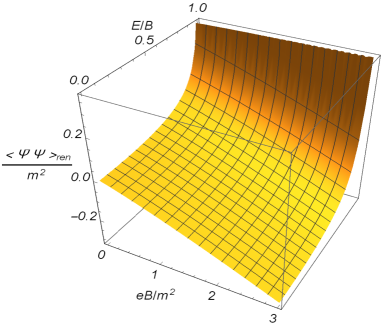
Figure 1: The renormalized fermion condensate in units of $m^{2}$, $\left\langle\overline{\Psi}\Psi\right\rangle_{\mathrm{ren}}/m^{2}$, versus $eB/m^{2}$ and $E/B$ for the field with $s=1$.

4 VEV of the energy-momentum tensor

In this Section, we consider another important characteristic of the fermionic vacuum, namely, the VEV of the energy-momentum tensor. The corresponding operator is given as

$$T_{\mu\nu}=\frac{1}{2}i\left[\bar{\Psi}\gamma_{(\mu}D_{\nu)}\Psi-\left(D_{(\mu}\bar{\Psi}\right)\gamma_{\nu)}\Psi\right],$$ (30)

where

$$D_{\mu}=\partial_{\mu}+ieA_{\mu},$$ (31)

and the brackets in the indices mean symmetrization over the included indices.

The corresponding VEV is written in the form of the mode sum

$$\left\langle T_{\mu\nu}\right\rangle=-\frac{i}{4}\sum_{\sigma}\sum_{\chi=-,+}\chi\left[\bar{\Psi}_{\sigma}^{\chi}\gamma_{(\mu}D_{\nu)}\Psi_{\sigma}^{\chi}-\left(D_{(\mu}\bar{\Psi}_{\sigma}^{\chi}\right)\gamma_{\nu)}\Psi_{\sigma}^{\chi}\right].$$ (32)

By using the mode functions given above it can be seen that the off-diagonal components of the energy-momentum tensor vanish. Therefore, let us consider the diagonal components of the energy-momentum tensor.

For the VEV of the energy density we get

$$\left\langle T_{00}\right\rangle=-\frac{1}{2}\sum_{\sigma}\int_{-\infty}^{+\infty}dp^{2}\sum_{\chi=-,+}\chi\left(p^{0\left(\chi\right)}-eA_{0}\right)\Psi_{\sigma}^{\chi\dagger}\Psi_{\sigma}^{\chi}.$$ (33)

Substituting the mode functions and using the orthogonality relation for the Hermite polynomials, we obtain the following expression for the VEV of the energy density:

$$\left\langle T_{00}\right\rangle=-\frac{eB}{2\pi}\sum_{n=0}^{\infty}g_{n}\left(B,\beta\right)\left(1+\frac{\beta}{\sqrt{1-\beta^{2}}}\frac{\left(n+1\right)eB}{2\left(n+1\right)eB\sqrt{1-\beta^{2}}+m^{2}}\right).$$ (34)

For the contribution of the zero mode (22) to the energy density we get

$$\left\langle T_{00}\right\rangle_{(0)}=-\frac{eB}{2\pi}\frac{m}{1-\beta^{2}}.$$ (35)

The total VEV of the energy density is expressed as

$$\left\langle T_{00}\right\rangle_{\mathrm{tot}}=-\frac{eB}{2\pi}\frac{m}{1-\beta^{2}}-\frac{eB}{2\pi}\sum_{n=0}^{+\infty}g_{n}\left(B,\beta\right)\left[1+\frac{\beta}{\sqrt{1-\beta^{2}}}\frac{\left(n+1\right)eB}{2\left(n+1\right)eB\sqrt{1-\beta^{2}}+m^{2}}\right].$$ (36)

This result is expressed in terms of the Hurwitz function

$$\left\langle T_{00}\right\rangle_{\mathrm{tot}} = \frac{eB}{2\pi}\frac{m}{1-\beta^{2}}\left\{-1+\frac{\left(1-\beta^{2}\right)^{-\frac{1}{4}}}{\sqrt{2}}\left[\frac{m\beta}{2\sqrt{eB}}\zeta\left(\frac{1}{2},u\right)\right.\right.$$ (37)

$$\left.\left.-\left(2+\frac{\beta}{1-\beta^{2}}\right)\left(1-\beta^{2}\right)^{\frac{3}{2}}\frac{\sqrt{eB}}{m}\zeta\left(-\frac{1}{2},u\right)\right]\right\}.$$

The vacuum energy density is the same for the fields with $s=1$ and $s=-1$.

In the case of the absence of electric and magnetic fields we have

$$\lim_{B,E\rightarrow 0}\left\langle T_{00}\right\rangle_{\mathrm{tot}}=\frac{m^{3}}{6\pi}.$$ (38)

Similar to the case of the fermion condensate we impose a renormalization condition that corresponds to the zero energy density in the limit $B,$ $E\rightarrow 0$. By taking into account (38), for the renormalized energy density one obtains

$$\left\langle T_{00}\right\rangle_{\mathrm{ren}} = \frac{eB}{2\pi}\frac{m}{1-\beta^{2}}\left\{-1+\frac{\left(1-\beta^{2}\right)^{-\frac{1}{4}}}{\sqrt{2}}\left[\frac{m\beta}{2\sqrt{eB}}\zeta\left(\frac{1}{2},u\right)\right.\right.$$ (39)

$$\left.\left.-\left(2+\frac{\beta}{1-\beta^{2}}\right)\left(1-\beta^{2}\right)^{\frac{3}{2}}\frac{\sqrt{eB}}{m}\zeta\left(-\frac{1}{2},u\right)\right]\right\}-\frac{m^{3}}{6\pi}.$$

In the special case of the zero electric field, this expression is simplified to

$$\left\langle T_{00}\right\rangle_{\mathrm{ren}}=-\frac{eB}{2\pi}\left[m+\sqrt{2eB}\zeta\left(-\frac{1}{2},1+\frac{m^{2}}{2eB}\right)\right]-\frac{m^{3}}{6\pi}.$$ (40)

In the limit when the electric field tends to its critical value, $E\rightarrow B$, one has $\beta\rightarrow 1$ and by using the asymptotic (25) for the leading term in the expansion of the energy density we find

$$\left\langle T_{00}\right\rangle_{\mathrm{ren}}\approx-\frac{m^{3}}{6\pi\left(1-\beta^{2}\right)^{\frac{3}{2}}}.$$ (41)

The ratio $\left\langle T_{00}\right\rangle_{\mathrm{ren}}/m^{3}$ is a function of the ratios $eB/m^{2}$ and $E/B$ (the same is the case for the spatial components). In Figure 2 the dependence of the energy density (in units of $m^{3}$) is plotted on the combinations $eB/m^{2}$ and $E/B$. As it is seen from the graph, the energy density is negative. The emergence of negative energy density in a quantum field theory is very legitimate. The renormalized energy density of a quantized field is obtained by the subtraction of divergent contribution and, in general, is not positive (see, e.g., [15]). Well known example is the energy density for the electromagnetic vacuum in the region between two parallel conducting plates (the Casimir effect) [16].

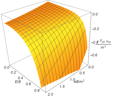
Figure 2: The renormalized VEV of the energy density in units of $m^{3}$, $\left\langle T_{00}\right\rangle_{\mathrm{ren}}/m^{3}$, as a function of $eB/m^{2}$ and $E/B$.

Now we consider the component

$$\left\langle T_{11}\right\rangle=-\frac{i}{4}\sum_{\sigma}\sum_{\chi=-,+}\chi\left[\Psi_{\sigma}^{\chi\dagger}\gamma^{0}\gamma_{1}\partial_{1}\Psi_{\sigma}^{\chi}-\left(\partial_{1}\Psi_{\sigma}^{\chi\dagger}\right)\gamma^{0}\gamma_{1}\Psi_{\sigma}^{\chi}\right].$$ (42)

With the mode functions from (13) this expression is transformed to

$$\left\langle T_{11}\right\rangle=-\frac{\left(eB\right)^{2}}{2\pi}\sqrt{1-\beta^{2}}\sum_{n=0}^{\infty}\frac{n+1}{g_{n}\left(B,\beta\right)}.$$ (43)

The contribution to the component $\left\langle T_{11}\right\rangle$ coming from the zero mode vanishes. As before, we write the corresponding expression in terms of the Hurwitz function:

$$\left\langle T_{11}\right\rangle=-\frac{\left(eB\right)^{\frac{3}{2}}}{2^{\frac{3}{2}}\pi}\left(1-\beta^{2}\right)^{\frac{1}{4}}\left[\zeta\left(-\frac{1}{2},u\right)-\frac{m^{2}}{2eB\sqrt{1-\beta^{2}}}\zeta\left(\frac{1}{2},u\right)\right].$$ (44)

Again, in the case of the absence of electric and magnetic fields we have the following limiting value:

$$\lim_{B,E\rightarrow 0}\left\langle T_{11}\right\rangle=-\frac{m^{3}}{6\pi}.$$ (45)

The renormalization condition described above leads to the renormalized VEV

$$\left\langle T_{11}\right\rangle_{\mathrm{ren}}=-\frac{\left(eB\right)^{\frac{3}{2}}}{2^{\frac{3}{2}}\pi}\left(1-\beta^{2}\right)^{\frac{1}{4}}\left[\zeta\left(-\frac{1}{2},u\right)-\frac{m^{2}}{2eB\sqrt{1-\beta^{2}}}\zeta\left(\frac{1}{2},u\right)\right]+\frac{m^{3}}{6\pi}.$$ (46)

In the problem with zero electric field the formula (46) is rewritten as

$$\left\langle T_{11}\right\rangle_{\mathrm{ren}}=-\frac{\left(eB\right)^{\frac{3}{2}}}{2^{\frac{3}{2}}\pi}\left[\zeta\left(-\frac{1}{2},1+\frac{m^{2}}{2eB}\right)-\frac{m^{2}}{2eB}\zeta\left(\frac{1}{2},1+\frac{m^{2}}{2eB}\right)\right]+\frac{m^{3}}{6\pi}.$$ (47)

For the asymptotic behavior of the VEV of the component $\left\langle T_{11}\right\rangle$ in the limit $\beta\rightarrow 1$ one obtains

$$\left\langle T_{11}\right\rangle_{\mathrm{ren}}\approx-\frac{m^{3}}{6\pi\sqrt{1-\beta^{2}}}.$$ (48)

It remains to consider the 22-component

$$\left\langle T_{22}\right\rangle=\frac{1}{2}\sum_{\sigma}\sum_{\chi=-,+}\chi\left(p^{2}+eBx^{1}\right)\Psi_{\sigma}^{\chi\dagger}\gamma^{0}\gamma_{2}\Psi_{\sigma}^{\chi}.$$ (49)

With the mode functions given above, this component is expressed as

$$\left\langle T_{22}\right\rangle=-\frac{\left(eB\right)^{2}}{2\pi\sqrt{1-\beta^{2}}}\sum_{n=0}^{\infty}\frac{n+1}{g_{n}\left(B,\beta\right)}.$$ (50)

Written in terms of the Hurwitz function, one gets

$$\left\langle T_{22}\right\rangle=-\frac{\left(eB\right)^{\frac{3}{2}}}{2^{\frac{3}{2}}\pi}\frac{1}{\left(1-\beta^{2}\right)^{\frac{3}{4}}}\left[\zeta\left(-\frac{1}{2},u\right)-\frac{m^{2}}{2eB\sqrt{1-\beta^{2}}}\zeta\left(\frac{1}{2},u\right)\right].$$ (51)

Taking into account that

$$\lim_{B,E\rightarrow 0}\left\langle T_{22}\right\rangle=-\frac{m^{3}}{6\pi},$$ (52)

for the renormalized VEV we obtain

$$\left\langle T_{22}\right\rangle_{\mathrm{ren}}=-\frac{\left(eB\right)^{\frac{3}{2}}}{2^{\frac{3}{2}}\pi}\frac{1}{\left(1-\beta^{2}\right)^{\frac{3}{4}}}\left[\zeta\left(-\frac{1}{2},u\right)-\frac{m^{2}}{2eB\sqrt{1-\beta^{2}}}\zeta\left(\frac{1}{2},u\right)\right]+\frac{m^{3}}{6\pi}.$$ (53)

In the absence of electric field $\left\langle T_{22}\right\rangle_{\mathrm{ren}}=\left\langle T_{11}\right\rangle_{\mathrm{ren}}$ which is a direct consequence of the symmetry and calculating the trace of the energy-momentum tensor from formulas (40), (47), (53) and passing to the $E\rightarrow 0$ limit, we will get the result given in [13] (the difference in the sign is due to the difference in the signature). Note that for $1-\beta^{2}\ll 1$ one has $\left\langle T_{22}\right\rangle_{\mathrm{ren}}\approx\left\langle T_{00}\right\rangle_{\mathrm{ren}}$ and $|\left\langle T_{11}\right\rangle_{\mathrm{ren}}|\ll|\left\langle T_{22}\right\rangle_{\mathrm{ren}}|$.

The Figure 3 displays the components $\left\langle T_{11}\right\rangle_{\mathrm{ren}}$ (left panel) and $\left\langle T_{22}\right\rangle_{\mathrm{ren}}$ (right panel) as functions of dimensionless combinations $eB/m^{2}$ and $E/B$. Both the components are positive for $E=0$ and with increasing $E$ they change the sign.

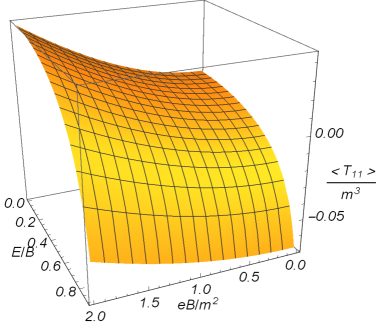
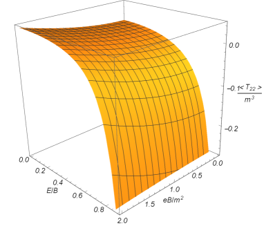
Figure 3: The dependence of the spatial components of the vacuum energy-momentum tensor (in units of $m^{3}$) on the ratios $eB/m^{2}$ and $E/B$.

In a graphene sheet, the long-wavelength description of electronic states can be formulated in terms of the Dirac theory of spinors in (2+1)-dimensional space-time, where the Fermi velocity plays the role of the speed of light. The expression for the fermion condensate and of the energy-momentum tensor in the corresponding model are obtained from the formulae given above by the replacements $\beta\rightarrow E/(v_{F}B)$ and $m\rightarrow$ $mv_{F}$ (for the generation of Dirac mass term in the effective description of graphene see, for example, [18]).

5 Conclusion

In this paper, we have investigated the massive fermionic quantum field localized on a plane in external constant and homogeneous electric and magnetic fields. The magnetic field is perpendicular to the plane and the electric field is parallel to the plane. For the evaluation of the fermionic vacuum characteristics, we have used the summation over the corresponding mode functions. Those functions are presented in section 2. The related energy spectrum and its features have been discussed in [2]. Here we investigate the fermion condensate and the VEV of the energy-momentum tensor. The renormalization procedure is based on the zeta function technique. We are interested in the effects induced by external electric and magnetic fields and an additional renormalization condition is imposed that requires zero expectation values in the absence of external fields. The renormalized fermion condensate is negative for zero electric field and becomes positive for the values of the electric field close to the critical value $E\rightarrow B$ ($\beta\rightarrow 1$). The vacuum energy density is always negative, whereas the vacuum stresses are positive in the region $E\ll B$ and negative for $1-(E/B)^{2}\ll 1$. For the values of the electric field near the critical value, $E\rightarrow B$ one has $|\left\langle T_{11}\right\rangle_{\mathrm{ren}}|\ll|\left\langle T_{22}\right\rangle_{\mathrm{ren}}|$ and $\left\langle T_{22}\right\rangle_{\mathrm{ren}}\approx\left\langle T_{00}\right\rangle_{\mathrm{ren}}$.

The analysis showed that in the presence of crossed uniform electric and magnetic fields, we have the following phenomena: the contraction and eventual collapse of the Landau level (see [2]), the changing sign of the condensate, and the negative energy density, which can be verified experimentally.

Another class of effects on the vacuum of (2+1)-dimensional fermions induced by magnetic fields have been discussed in [19, 20] for cylindrical and toroidal topologies of the background space. In those references, the influence of the magnetic flux threading the compact dimensions is studied and the effect has topological nature (of the Aharonov-Bohm type). Similar effects for conical geometry with edges were considered in [21]-[24]. In these geometries, the local characteristics of the vacuum state are periodic functions of the magnetic flux with the period equal to the quantum of flux.

References

- [1] P. A. M. Dirac, Proc. Roy. Soc., A 117, 610 (1928), I. I. Rabi, Zeits. Phys., 49, 7 (1928), F. Sauter, Zeits. Phys. 69, 742 (1931), D. M. Volkow, Zeits. Phys. 94, 25 (1935), P. J. Redmond, Journ. Math. Phys. 6, 1163 (1965), V. Canuto, C. Chiuderi, Nuovo Cimento Letters 2, 223 (1969).
- [2] V. Lukose, R. Shankar, G. Baskaran, Phys. Rev. Lett. 98, 116802 (2007).
- [3] I. A. Shovkovy, Lect. Notes Phys. 871, 13 (2013).
- [4] V. P. Gusynin, V. A. Miransky, I.A. Shovkovy, Phys. Rev. Lett. 73, 3499 (1994).
- [5] A. Raya, E. Reyes, Phys. Rev. D 82, 016004 (2010).
- [6] J. A. Sanchez-Monroy, C. T. Quinbay, arxiv: 1903.071802 [hep-th].
- [7] P. Cea and L. Tedesco, J. Phys. G: Nucl. Part. Phys. 26, 411 (2000).
- [8] V. R. Khalilov, Eur. Phys. J. C 79, 196 (2019).
- [9] J. J. Lenz, M. Mandl, A. Wipf, Phys. Rev. D 107, 094505 (2023).
- [10] V. P. Gusynin, V. A. Miransky, I. A. Shovkovy, Phys. Rev. D 52, 4718 (1995).
- [11] H. T. Feng et al, Sci. China-Phys. Mech. Astrom. 56, 1116 (2013).
- [12] F. W. J. Olver, D. W. Lozier, R. F. Boisvert, C. W. Clark, NIST Handbook of Mathematical Functions (Cambridge University Press, 2010).
- [13] W. Dittrich, H. Gies, Phys. Lett. B 392, 182 (1997).
- [14] A. A. Saharian, E. R. Bezerra de Mello, A. S. Kotanjyan, et al., Astrophysics 64, 529 (2021).
- [15] L. H. Ford, Int. J. Mod. Phys. A 25, 2355 (2010).
- [16] M. Bordag, U. Mohidden, G. Klimchitskaya, V. Mostepanenko, Advances in the Casimir effect, Oxford University Press, 2009.
- [17] A. H. Castro Neto, F. Guinea, N. M. R. Peres, K. S. Novoselov, A. K. Geim, Rev. Mod. Phys. 81, 109 (2009).
- [18] V. P. Gusynin, S. G. Sharapov, J. P. Carbotte, Int. J. Mod. Phys. B 21, 4611 (2007).
- [19] S. Bellucci, A. A. Saharian, Phys. Rev. D 79, 085019 (2009).
- [20] S. Bellucci, A. A. Saharian, V. M. Bardeghyan, Phys. Rev. D 82, 065011 (2010).
- [21] E. R. Bezerra de Mello, V. Bezerra, A. A. Saharian, V. M. Bardeghyan, Phys. Rev. D 82, 085033 (2010).
- [22] S. Bellucci, E. R. Bezerra de Mello, A. A. Saharian, Phys. Rev. D 83, 085017 (2011).
- [23] E. R. Bezerra de Mello, F. Moraes, A. A. Saharian, Phys. Rev. D 85, 045016 (2012).
- [24] S. Bellucci, I. Brevik, A. A. Saharian, H. G. Sargsyan, Eur. Phys. J. C 80, 281 (2020).