Learning Variable Impedance Skills from Demonstrations with Passivity Guarantee

Abstract

Robots are increasingly being deployed not only in workplaces but also in households. Effectively execute of manipulation tasks by robots relies on variable impedance control with contact forces. Furthermore, robots should possess adaptive capabilities to handle the considerable variations exhibited by different robotic tasks in dynamic environments, which can be obtained through human demonstrations. This paper presents a learning-from-demonstration framework that integrates force sensing and motion information to facilitate variable impedance control. The proposed approach involves the estimation of full stiffness matrices from human demonstrations, which are then combined with sensed forces and motion information to create a model using the non-parametric method. This model allows the robot to replicate the demonstrated task while also responding appropriately to new task conditions through the use of the state-dependent stiffness profile. Additionally, a novel tank based variable impedance control approach is proposed to ensure passivity by using the learned stiffness. The proposed approach was evaluated using two virtual variable stiffness systems. The first evaluation demonstrates that the stiffness estimated approach exhibits superior robustness compared to traditional methods when tested on manual datasets, and the second evaluation illustrates that the novel tank based approach is more easily implementable compared to traditional variable impedance control approaches.

I Introduction

The use of robots has become increasingly widespread in various fields including manufacturing and rehabilitation [1, 2]. Due to their ability to perform complex manipulation tasks in unknown and unstructured environments that make fixed coding impractical. It is an appropriate approach to use Learning from demonstration (LfD) for the present case, as LfD is an intuitive and user-friendly method that allows robots to implicitly learn task constraints and acquire manipulation skills through demonstrations [3], thus avoiding hard coding for different tasks. Most LfD methods mainly focus on learning motion trajectories [4, 5]; for robots operating in unknown and unstructured environments, however, learning motion trajectories alone is not sufficient. Extending robot learning capabilities to force and impedance domains [6, 7] is critical for robots working in dynamic environments.

This paper proposes a framework that learns variable impedance skills from demonstrations while ensuring passivity. The proposed learning framework estimates demonstrated stiffness from demonstrations and implements variable impedance control using a novel tank-based approach that guarantees passivity with the learned stiffness. The main contributions of this paper are listed below:

• A effectiveness stiffness estimating method is proposed that can estimate the demonstrate stiffness from the demonstrations, regardless of whether the damping information is known in advance.

• A non-parametric method is utilized to construct a function relating stiffness with motion and force information, thereby reproducing the estimated stiffness. This approach incorporates more information than solely considering force information, resulting in higher reproduction accuracy and improved generalization performance.

• A novel tank-based approach for implementing the variable impedance control is proposed, which ensures passivity of the system when tracking errors are below a certain threshold. If passivity cannot be maintained, setting the stiffness velocity to zero can restore the system back to a passive state.

The paper is structured as follows: In Section II, the related works are presented. Section III presents the effectiveness stiffness estimating method, the mode for relating stiffness with motion and force information, and the novel tank-based variable impedance control method. In Section IV, the performances of this methods are evaluated by simulation. In Section V, the conclusion is made.

II RELATED WORK

Humans possess an exceptional ability to adapt their stiffness when interacting with complex environments during manipulation tasks. This adaptability allows them to effectively control their level of stiffness or resistance based on the specific requirements of the task and the characteristics of the environment. Previous research has focused on understanding how humans modulate impedance while interacting with their environment and transferring these skills to robots [8, 9]. However, previous robot learning capabilities did not include automatic modification of impedance control parameters to respond to unforeseen situations. Recently, there has been a surge of interest in robot learning approaches for modeling variable impedance skills, in tasks where a robot needs to physically interact with the environment, including humans.

Researchers have developed various methods for generating variable stiffness parameters for the controller based on either task rules, movement models derived from human demonstration, or reinforcement learning [10, 11, 12, 13]. Based on the rule of assist-as-need, [14] utilizes the electromyography (sEMG) signals from muscles related to the joint to estimate both joint torque and quasi-stiffness of human in order to map to the voluntary efforts of the human subject. Then the manually designed control strategy adjusts the degree of assistance by varying the stiffness for variable impedance control. Specifically, When the robot detects a need to assist the human user, the stiffness parameter of the controller is set to a higher value, on the other hand, when the system detects that the human user is attempting to move actively, the stiffness parameter is set to be a lower value. In [15], a controller for coupled human-robot systems is proposed to improve stability and agility while reducing effort required by the human user. The controller achieves this goal by dynamically adjusting both damping and stiffness. Specifically, the controller applies robot damping within a range of negative to positive values to add or dissipate energy depending on the intended motion of the user. The authors in [16, 17, 18, 19, 20], developed a variable impedance controller that uses the time-varying stiffness parameters estimated from human demonstrations. By utilizing the estimated stiffness parameters, the controller allows the robot to adapt its impedance or stiffness during interactions, mimicking the natural and intuitive behavior observed in humans. In [21], the authors propose a method for learning a policy that enables robots to generate behaviors in the presence of contact uncertainties. The approach involves learning two key components: the output impedance and the desired position in joint space. Additionally, an additional reward term regularizer is introduced to enhance the learning process. The output impedance refers to the robot’s ability to modulate its interaction forces and stiffness during contact with the environment. By learning the appropriate output impedance, the robot can effectively adapt to different contact uncertainties, ensuring stable and controlled interactions.

The preceding studies demonstrated various methods for designing variable stiffness profiles that enable robots to perform different interaction tasks. The variable impedance controller enhances the robot’s ability to interact with its environment by dynamically adjusting its stiffness based on the task requirements and environmental conditions. However, it has been observed that the use of variable stiffness parameters in impedance controllers can potentially compromise the stability of physical human-robot interactions [22, 23]. The passivity theory, which is widely used in the field of robotics, provides an energy-based perspective for evaluating the coupled stability of physical human-robot interaction. This theory allows for an analysis of the energy flow and exchange between the robot and the human, offering a valuable framework for designing robot behaviors that are both safe and effective [24]. In the context of physical human-robot interaction, the passivity of a robot-human system is determined by comparing the energy stored in the robot with the external energy injected by the environment, which is typically attributed to the human. A passive system is characterized by the condition that the energy stored in the robot remains consistently lower than the external energy injected by the environment. This definition of passivity ensures that the robot does not generate additional energy and remains stable even in the absence of any external forces. By maintaining a lower energy level than that injected by the human, the robot avoids becoming energetically dominant and guarantees that the interaction remains safe and controlled. In [22], the authors introduce a novel Lyapunov candidate function that offers more relaxed stability conditions for a system, which potentially expands the range of system behaviors that can be considered stable. However, the proposed conditions may not be sufficient for robots operating in unstructured environments. To ensure the stability and robustness of robots operating in unstructured environments, additional considerations and techniques may be necessary. The authors in [23] introduce a virtual energy-storing tank that can absorb and store the dissipation energy from the robot. When the virtual tank is available, it compensates for any additional energy generated by the robot and provides a more straightforward and practical way for preserving the passivity of the robot-human system. By effectively compensating for the excess energy generated by the robot, the virtual tank ensures that the energy balance within the system is maintained. This compensation mechanism simplifies the design and control of the robot, as it provides a approach to regulate and manage the energy flow without compromising the passivity requirements.

III Proposed Approach

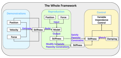
Figure 1: The framework for learning variable stiffness from demonstrations and implementing variable impedance control.

This section introduces a novel architecture for Programming by Demonstration (PbD) that not only facilitates the learning and replication of variable impedance skills in cooperative tasks but also ensures passivity. Incorporating passivity into the architecture is critical because when transferring human’s variable stiffness skills, it ensures that the robot can effectively learn and replicate these skills while maintaining stability and safety.

III-A Interaction Model

Human beings demonstrate a remarkable ability to apply appropriate force to achieve desired dynamic relationships with their environment. This capacity finds a counterpart in impedance control, a highly effective method for regulating interaction behaviors between robots and their working environment. By learning from human demonstrations, robots can acquire the ability to perform tasks that require adaptive impedance control.

Given that the majority of interactions take place within the task space, they predominantly involve the utilization of the robots’ end-effector. Specifically, the movement of a robot’s end-effector within the task space can be effectively represented as a mass unit influenced by two primary factors: interaction forces denoted as $\boldsymbol{f}^{e}$, and the control input denoted as $\boldsymbol{f}^{c}$. This modeling approach is supported by [26]:

$$\boldsymbol{H}\ddot{\boldsymbol{x}}=\boldsymbol{f}^{e}+\boldsymbol{f}^{c},$$ (1)

where $\ddot{\boldsymbol{x}}$ denotes the acceleration of the motion and $\boldsymbol{H}$ denotes a positive definite matrix that remains unchanged for the task. By configuring the motion control forces as $\boldsymbol{f}^{c}$ in the presence of an interaction force $\boldsymbol{f}^{e}$, the desired dynamics can be achieved.

Impedance control allows the modeling of the robot’s motion during interaction as a virtual mass-spring-damper (MSD) system at each time step $t$. Specifically, assuming that the reference motions are available, which can be designed manually or learned from demonstrations, the equation of impedance motion can be expressed as follows:

$$\boldsymbol{H}(\ddot{\boldsymbol{x}}_{t}-\ddot{\boldsymbol{x}}^{r}_{t})+\boldsymbol{K}_{t}(\boldsymbol{x}_{t}-\boldsymbol{x}^{r}_{t})+\boldsymbol{D}_{t}(\dot{\boldsymbol{x}}_{t}-\dot{\boldsymbol{x}}^{r}_{t})=\boldsymbol{f}_{t}^{e},$$ (2)

where $\boldsymbol{x}_{t}^{r}$, $\boldsymbol{\dot{x}}_{t}^{r}$ $\boldsymbol{\ddot{x}}_{t}^{r}$, $\boldsymbol{K}_{t}$, and $\boldsymbol{D}_{t}$, represent position, velocity, acceleration of the reference trajectory, as well as the full stiffness matrix, damping matrix for the virtual MSD system, respectively. Conversely, $\boldsymbol{x}_{t}$, $\dot{\boldsymbol{x}}_{t}$, $\ddot{\boldsymbol{x}}_{t}$, and $\boldsymbol{f}_{t}^{e}$ denote the position, velocity, acceleration, and interaction forces of the real motion, respectively.

$\dot{\boldsymbol{x}}_{t}$ and $\ddot{\boldsymbol{x}}_{t}$ are the first and second time derivatives of ${\boldsymbol{x}}_{t}$ that can be easily computed once the position and time information are acquired, and the interaction forces $\boldsymbol{f}_{t}^{e}$ can be directly measured using a force sensor mounted on the robot’s end-effector. By using $\boldsymbol{e},\dot{\boldsymbol{e}},\ddot{\boldsymbol{e}}$ to represent the position, velocity, and acceleration errors between real motions and reference motions, equation (2) can be reformulated as:

$$\boldsymbol{H}\ddot{\boldsymbol{e}}_{t}+\boldsymbol{K}_{t}\boldsymbol{e}_{t}+\boldsymbol{D}_{t}\dot{\boldsymbol{e}}_{t}=\boldsymbol{f}_{t}^{e}.$$ (3)

Subsequently, the robot’s behavior can be customized by modifying the stiffness within the refer trajectories in the interaction model (2). To attain an ideal human-like behavior, the variables $\boldsymbol{K}_{t}$ can be acquired through demonstrations conducted by human teachers. By observing and recording the actions and behaviors of skilled human teachers, the robot can learn and extract the desired variable parameters $\boldsymbol{K}_{t}$ that represent the stiffness characteristics of the human.

III-B Stiffness Estimation from Demonstrations

To obtain the full stiffness matrix $\boldsymbol{K}_{t}$, experts have explored various methods. One approach utilized by [16] involves the use of the Gaussian mixture model (GMM) to cluster the demonstrated data and estimated $\boldsymbol{K}_{t}$ by obtaining the inverse of the position covariance. However, this approach requires multiply demonstrations and cannot be applied to tasks where the robot’s end-effector is constrained to follow a single path. Another approach, as described by [18] utilized the electromyography (sEMG) signals to estimate stiffness. This approach calculates the activation level of human muscles and offers the advantage of being cost-effective while providing real-time estimation. In a similar vein, [19] specifically emulates imitates the underlying the inherent transformation within the muscular and skeletal systems. They employs the model-based approach to estimate the joint torque and joint stiffness simultaneously without additional calibration procedures. However, the sEMG based approaches are highly sensitive to noise and individual differences.

A different approach proposed by [20] uses the neural network to estimate the stiffness and damping from the demonstrations, based on the states of end-effector and the interaction force. Although this method can easily generalize to different states, training the neural network is time consuming and the accuracy is not always satisfactory. In contrast, [17] proposes an algorithm that uses the least squares method with the nearest positive definite matrix (SPD) method to estimate the stiffness with a sliding window at each time step quickly. However, a predetermined damping value is acquired by this algorithm, which is not known in the real demonstrations. Therefore, the accuracy of the estimated stiffness relies on the empirically designed value of the damping. Inspired by [17], a novel stiffness estimation algorithm that inherit the highly effectiveness of [17] while do not need to know the damping.

The algorithm proposed by [17] is introduced firstly. In human demonstration, with the reference trajectories, the presented data in the demonstrations include position, velocity, acceleration, and external force vectors, respectively. Then to estimate the full stiffness matrix at each time step $t$, [17] employs a sliding window $L$ that moves along the demonstration data. In real experiments, a small sliding window is employed to treat stiffness as an invariant within a short period of time.

Equation (3) can be also expressed as:

$$\boldsymbol{K}_{t}\boldsymbol{e}_{t}=\boldsymbol{f}_{t}^{e}-\boldsymbol{H}_{t}\boldsymbol{\ddot{e}}_{t}-\boldsymbol{D}_{t}\boldsymbol{\dot{e}}_{t}.$$ (4)

By defining $\boldsymbol{f}_{t}^{e}-\boldsymbol{H}_{t}\boldsymbol{\ddot{e}}_{t}-\boldsymbol{D}_{t}\boldsymbol{\dot{e}}_{t}$ as $\tilde{\boldsymbol{y}}_{t}$ and $\boldsymbol{e}_{t}$ as $\tilde{\boldsymbol{x}}_{t}$, equation (4) becomes:

$$\boldsymbol{K}_{t}\tilde{\boldsymbol{x}}_{t}=\tilde{\boldsymbol{y}}_{t}.$$ (5)

Hence, a rough approximation stiffness $\boldsymbol{\hat{B}}_{t}$ at each step can be calculated by using the least squares method. Subsequently, a nearest-SPD matrix is calculated to represent the estimated stiffness. To calculate the nearest-SPD matrix, $\boldsymbol{B}_{t}=\frac{\boldsymbol{\hat{B}}_{t}+\boldsymbol{\hat{B}}^{\mathrm{T}}_{t}}{2}$ is first computed. Next, $\boldsymbol{B}_{t}$ is decomposed as $\boldsymbol{B}_{t}=\boldsymbol{U}_{t}\boldsymbol{S}_{t}\boldsymbol{V}_{t}^{\mathrm{T}}$. The resulting matrices $\boldsymbol{V}_{t}$ and $\boldsymbol{S}_{t}$ are then used to create a new matrix as $\boldsymbol{L}_{t}=\boldsymbol{V}_{t}\boldsymbol{S}_{t}\boldsymbol{V}_{t}^{\mathrm{T}}$. Finally, the estimated stiffness is represented as $\boldsymbol{\hat{K}}_{t}=\frac{\boldsymbol{B}_{t}+\boldsymbol{L}_{t}}{2}$ if it is a SPD matrix. if $\boldsymbol{\hat{K}}_{t}$ is not SPD, the eigenvalues are adjusted to be positive, then the estimated stiffness is a $N$ dimensional symmetric and positive definite matrix.

It can be seen that to estimate the full stiffness matrix from the demonstrations, the damping must be predetermined by using the method proposed in [17]. However, in real experiments, the demonstrations can provide state information but not damping, meaning that both stiffness and damping are unknown before estimating the stiffness.

To handle this problem, a modified method is proposed in this paper that can estimate both stiffness and damping from the demonstrations. The method inherits the effectively of [17] while also utilizing the prior knowledge that $\boldsymbol{K}_{t}$ is a symmetric matrix, resulting in a more reliable stiffness estimation from demonstrations.

The most commonly available variable impedance control assumes that the damping is constant or corresponds to the stiffness matrices, thereby maintaining critical damping of the system. Then the damping in demonstrations can be also assumed to be constant or correspond to stiffness.

Firstly, assume that the damping is a constant and known, $\boldsymbol{\hat{B}}_{t}$ for equation (5) can be calculated as:

$$\boldsymbol{\hat{B}}_{t}=\tilde{\boldsymbol{y}}_{t}\tilde{\boldsymbol{x}}^{\mathrm{T}}_{t}(\tilde{\boldsymbol{x}}_{t}\tilde{\boldsymbol{x}}^{\mathrm{T}}_{t})^{-1},$$ (6)

or

$$\boldsymbol{\hat{B}}_{t}=\tilde{\boldsymbol{y}}_{t}(\tilde{\boldsymbol{x}}^{\mathrm{T}}_{t}\tilde{\boldsymbol{x}}_{t})^{-1}\tilde{\boldsymbol{x}}^{\mathrm{T}}_{t}.$$ (7)

Taking equation (6) for example, let $\boldsymbol{T}_{t}$ represents $\tilde{\boldsymbol{y}}_{t}\tilde{\boldsymbol{x}}_{t}^{\mathrm{T}}$, The results of (6) can be reformulated as

$$B_{t_{1}}||B_{t_{2}}||\cdots||B_{t_{N^{2}}}=T_{t_{1}}||T_{t_{2}}||\cdots||T_{t_{N^{2}}}\boldsymbol{P},$$ (8)

where the symbol $||$ denotes concatenation, and for $i=1,2,\cdots,N^{2}$ with $\boldsymbol{B}_{t}$ and $\boldsymbol{T}_{t}$ denote for the i-th element in $\boldsymbol{B}_{t_{i}}$ and $\boldsymbol{T}_{t_{i}}$, respectively. The index in the matrix increases from left to right and top to bottom.

$$\boldsymbol{P}=\begin{bmatrix}(\tilde{\boldsymbol{x}}_{t}\tilde{\boldsymbol{x}}_{t}^{\mathrm{T}})^{-1}&\boldsymbol{0}&\cdots&\boldsymbol{0}\\ \boldsymbol{0}&(\tilde{\boldsymbol{x}}_{t}\tilde{\boldsymbol{x}}_{t}^{\mathrm{T}})^{-1}&\cdots&\boldsymbol{0}\\ \vdots&\vdots&\ddots&\vdots\\ \boldsymbol{0}&\cdots&\boldsymbol{0}&(\tilde{\boldsymbol{x}}_{t}\tilde{\boldsymbol{x}}_{t}^{\mathrm{T}})^{-1}\end{bmatrix},$$ (9)

where $(\tilde{\boldsymbol{x}}_{t}\tilde{\boldsymbol{x}}_{t}^{\mathrm{T}})^{-1}$ is a $N\times N$ matrix while $\boldsymbol{P}$ is a $N^{2}\times N^{2}$ matrix. Therefore, directly using the least squares method is equivalent to first use $\tilde{\boldsymbol{x}}_{t}$ in equation (5) times $N\times N$ $N\times N$ matrices as:

$$\begin{bmatrix}1&0&\cdots&0\\ 0&0&\cdots&0\\ \vdots&\vdots&\ddots&\vdots\\ 0&\cdots&0&0\end{bmatrix},\begin{bmatrix}0&1&\cdots&0\\ 0&0&\cdots&0\\ \vdots&\vdots&\ddots&\vdots\\ 0&\cdots&0&0\end{bmatrix},\cdots,\begin{bmatrix}0&0&\cdots&0\\ 0&0&\cdots&0\\ \vdots&\vdots&\ddots&\vdots\\ 0&\cdots&0&1\end{bmatrix},$$

to acquire $N\times N$ vectors, then use the least squares method to calculate the weights for each calculated vectors, which can recombine into the $\boldsymbol{B}_{t}$. However, the $N\times N$ matrices are not symmetry, which means that the recombined matrix is unlikely to be symmetric. In this paper the modified method is proposed to change these matrices, whereby $\tilde{\boldsymbol{x}}_{t}$ in equation (5) first times $N(N+1)/2$ $N\times N$ symmetry matrices that are denoted as $\boldsymbol{M}_{1}$ to $\boldsymbol{M}_{N(N+1)/2}$. The matrices are constructed as follows:

$$\begin{bmatrix}1&0&\cdots&0\\ 0&0&\cdots&0\\ \vdots&\vdots&\ddots&\vdots\\ 0&\cdots&0&0\end{bmatrix},\begin{bmatrix}0&1&\cdots&0\\ 1&0&\cdots&0\\ \vdots&\vdots&\ddots&\vdots\\ 0&\cdots&0&0\end{bmatrix},\cdots,\begin{bmatrix}0&0&\cdots&0\\ 0&0&\cdots&0\\ \vdots&\vdots&\ddots&\vdots\\ 0&\cdots&0&1\end{bmatrix}.$$

By times these matrices, $N(N+1)/2$ vectors are acquired. Equation (5) can be reformulated as:

$$\sum_{i=1}^{N(N+1)/2}w^{t}_{i}\boldsymbol{M}_{i}\tilde{\boldsymbol{x}}_{t}=\tilde{\boldsymbol{y}}_{t},$$ (10)

where $w^{t}_{i}$ are the weight to be calculated, where $i$ ranges from $1$ to $N(N+1)/2$. In equation (10), only the weights $w^{t}_{1},w^{t}_{2},...,w^{t}_{N(N+1)}$ are unknown and can be estimated by using the least squared. Once determined, they can be combined with $\boldsymbol{M}_{i}$ to obtain an approximation of the stiffness as follows:

$$\boldsymbol{B}_{t}=\sum_{i=1}^{N(N+1)/2}w^{t}_{i}\boldsymbol{M}_{i}.$$ (11)

However, there is still a possibility that the combined matrices may not be positive definite, and the nearest-SPD matrix method is still need to be applied to $\boldsymbol{B}_{t}$ to get an estimation of stiffness. The proposed method estimates fewer unknown parameters than direct least squares, which suggests that it has the potential to achieve higher accuracy when estimating stiffness from demonstrations.

Secondly, assuming that the damping value is an unknown constant, which is more likely in real experiments. The stiffness is still decomposed using the method described earlier, which involves acquiring $N(N+1)/2$ unknown parameters. Next, all $N(N+1)/2+1$ parameters, including $N(N+1)/2$ unknown parameters and the unknown damping constant, are all estimated using the least squares method. Subsequently, the estimated stiffness is acquired by recombining matrices with the calculated parameters and applying the nearest-SPD method.

Thirdly, assume that the damping is unknown but varies in correspondence with the stiffness, which means that assuming the demonstrations are critical damped. In other words, the stiffness and damping matrices are SPD and satisfy that:

$$\begin{cases}\boldsymbol{K}_{t}=\boldsymbol{T}_{t}^{\mathrm{T}}\boldsymbol{\Lambda_{t}}\boldsymbol{T}_{t},\\ \boldsymbol{D}_{t}=\boldsymbol{T}_{t}^{\mathrm{T}}(\zeta\boldsymbol{\Lambda^{\frac{1}{2}}_{t}})\boldsymbol{T}_{t},\\ \end{cases}$$ (12)

where $\boldsymbol{T}_{t}$ and $\boldsymbol{\Lambda}$ are the eigenvector and eigenvalue of the $\boldsymbol{K}_{t}$, and $\zeta\in\mathbb{R}^{+}$ is a manually designed parameter.

Estimating the full stiffness matrix by decomposing stiffness and damping using the $N(N+1)/2$ matrices described earlier and estimating the $N(N+1)$ unknown parameters using least squares often fails to produce good results because it does not satisfy the constraints between $\boldsymbol{K}_{t}$ and $\boldsymbol{D}_{t}$.

An alternative approach is to first estimate stiffness by assuming that damping is an unknown constant, and then calculate the corresponding damping using the estimated stiffness. This calculated damping can be substituted into equation (3) to estimate an iterative stiffness. The corresponding damping can be recalculated, and this process can be repeated several times to obtain the estimated stiffness.

In addition, during reproduction, $\boldsymbol{D}_{t}$ can be chosen by values learned from demonstrations or based on the desired response (e.g., critical damping) of the interaction system (3) chosen by experts.

III-C Stiffness Learning and Reproduction

The successful completion of most manipulation tasks relies heavily on the ability to perceive both force and position. Therefore, in this paper, the variable impedance skills are learned and reproduced based on interaction forces and position. GMMs are highly effective at establishing relationship between different variables, but their performance may be unsatisfactory when only one demonstration is provided. To face the conditions that either one or more demonstrations are provided, in this paper, $\boldsymbol{K}_{t}$ is first performed a Cholesky decomposition as $\boldsymbol{K}_{t}=\boldsymbol{L}_{t}^{\mathrm{T}}\boldsymbol{L}_{t}$, where $\boldsymbol{L}_{t}$ a lower triangular matrix and then the vectorization of $\boldsymbol{L}_{t}$ is modeled as:

$$\tilde{\boldsymbol{L}}_{t}=\Theta(\boldsymbol{s}_{t})^{\mathrm{T}}\boldsymbol{w}.$$ (13)

where $\Theta(\boldsymbol{s}_{t})$ is a vector of basis functions that depend on $\boldsymbol{s}_{t}$, which is the concatenated of force $\boldsymbol{f}_{t}^{e}$ and position $\boldsymbol{x}_{t}$ as $(\boldsymbol{f}_{t}^{e^{\mathrm{T}}}||\boldsymbol{x}_{t}^{\mathrm{T}})^{\mathrm{T}}$, and $\boldsymbol{w}$ is a weight vector to be learned. Therefore, after estimating stiffness and calculating the $\boldsymbol{L}_{t}$ from demonstration, the model can be obtained by minimizing the following objective function:

$$J(\boldsymbol{w})=\frac{1}{2}\sum_{n=1}^{N_{d}}\sum_{t=1}^{t_{m}}\begin{Bmatrix}\boldsymbol{w}^{\mathrm{T}}\Theta(\boldsymbol{s}_{t})_{n}-(\boldsymbol{f}_{t}^{e^{\mathrm{T}}}||\boldsymbol{x}_{t}^{\mathrm{T}})^{\mathrm{T}}_{n}\end{Bmatrix}^{2}+\frac{1}{2}\lambda\boldsymbol{w}^{\mathrm{T}}\boldsymbol{w},$$ (14)

where $\lambda$ is a positive constant to circumvent over-fitting, $n$ denotes the index of a demonstration, $t_{m}$ is the total number of samples in one demonstration and $N_{d}$ represents the total number of demonstrations.

The optimal solutions of the objective function can been represented as [25]:

$$\boldsymbol{w}^{*}=\Theta(\Theta^{\mathrm{T}}\Theta+\lambda I)^{-1}(\boldsymbol{f}^{e^{\mathrm{T}}}||\boldsymbol{x}^{\mathrm{T}})^{\mathrm{T}},$$ (15)

where $\Theta=[\Theta(\boldsymbol{s}_{1}),\Theta(\boldsymbol{s}_{2})\cdots,\Theta(\boldsymbol{s}_{N_{d}t_{N}})]$, $I$ is the $N_{d}t_{N}$-dimensional identity matrix and with a bit abuse of notations, $\boldsymbol{f}^{e}$ and $\boldsymbol{x}$ mean concatenating all the elements of force and position in demonstrations, respectively. Substitute the optimal $\boldsymbol{w}^{*}$ into (13), the vector $\tilde{\boldsymbol{L}}$ can be calculated as:

$$\tilde{\boldsymbol{L}}_{t}=\Theta(\boldsymbol{s}_{t})^{\mathrm{T}}\Theta(\Theta^{\mathrm{T}}\Theta+\lambda\boldsymbol{I})^{-1}(\boldsymbol{f}^{e^{\mathrm{T}}}||\boldsymbol{x}^{\mathrm{T}})^{\mathrm{T}}$$ (16)

To avoid the explicit definition of the basis functions in (16), the kernel trick is used to express the inner product as follows:

$$\begin{split}\boldsymbol{Ker}=\\ \begin{bmatrix}ker(\boldsymbol{s}_{1},\boldsymbol{s}_{1})&ker(\boldsymbol{s}_{1},\boldsymbol{s}_{2})&\cdots&ker(\boldsymbol{s}_{1},\boldsymbol{s}_{N_{d}t_{m}})\\ ker(\boldsymbol{s}_{2},\boldsymbol{s}_{1})&ker(\boldsymbol{s}_{2},\boldsymbol{s}_{2})&\cdots&ker(\boldsymbol{s}_{2},\boldsymbol{s}_{N_{d}t_{m}})\\ \vdots&\vdots&\ddots&\vdots\\ ker(\boldsymbol{s}_{N_{d}t_{m}},\boldsymbol{s}_{1})&ker(\boldsymbol{s}_{N_{d}t_{m}},\boldsymbol{s}_{2})&\cdots&ker(\boldsymbol{s}_{N_{d}t_{m}},\boldsymbol{s}_{N_{d}t_{m}})\end{bmatrix}\end{split}$$ (17)

where $ker(\boldsymbol{s}_{i},\boldsymbol{s}_{j})=\Theta(\boldsymbol{s}_{i})^{\mathrm{T}}\Theta(\boldsymbol{s}_{j})\quad\forall i,j\in[1,2\cdots,{N_{d}t_{m}}]$.

Thus, equation (16) can be reformulated as follows:

$$\tilde{\boldsymbol{L}}=\boldsymbol{ker}^{*}(\boldsymbol{Ker}+\lambda\boldsymbol{I})^{-1}(\boldsymbol{f}^{e^{\mathrm{T}}}||\boldsymbol{x}^{\mathrm{T}})^{\mathrm{T}},$$ (18)

where $\boldsymbol{ker}^{*}=[ker(\boldsymbol{s},\boldsymbol{s}_{1}),ker(\boldsymbol{s},\boldsymbol{s}_{2})\cdots,ker(\boldsymbol{s},\boldsymbol{s}_{N_{d}t_{m}})].$

The kernel function is designed as:

$$ker(\boldsymbol{s}_{i},\boldsymbol{s}_{j})=\boldsymbol{s}_{i}^{\mathrm{T}}\boldsymbol{s}_{j}e^{(-h\left\|(\boldsymbol{s}_{i}-\boldsymbol{s}_{j})\right\|^{2})},$$ (19)

where $h$ is a manually designed constant. Hence, when the input is $\boldsymbol{s}=\boldsymbol{0}$, it follows that $ker(\boldsymbol{s},\boldsymbol{s}_{j})=\boldsymbol{0}$. Therefore, when acquiring the position and interaction force, the vectorization of $\tilde{\boldsymbol{L}}$ is calculated from (19), and the lower triangular matrix $\boldsymbol{L}$ can be recombination from the vectorization of $\tilde{\boldsymbol{L}}$, afterwards, the stiffness is calculated as $\boldsymbol{K}=\boldsymbol{L}^{\mathrm{T}}\boldsymbol{L}$ that satisfies the symmetric and positive definite (SPD) constraints.

The purpose of reproducing the stiffness matrix is to shape the compliance of the robot like that of the human teacher and the control torque $\boldsymbol{f}^{c}$ in (1) for the robot can be calculated with the chosen $\boldsymbol{K}^{v}$, then transformed to joint torques $\boldsymbol{\tau}$ of the robot using the Jacobian transpose $J^{\mathrm{T}}$ as follows: $\boldsymbol{\tau}=J^{\mathrm{T}}\boldsymbol{f}^{c}$. However, directly applying the learned stiffness for interaction tasks can potentially lead to instability or unsafe behavior in the system. To address this issue, the next section introduces a novel tank-based approach that ensures the passivity of the system.

III-D A Novel Tank-Based Approach

The elegant tank-based approach is founded upon a sound energy-based idea. The central concept of the virtual tank involves the storage of dissipated energy by the variable impedance system, and the extraction of stored energy to compensate for nonpassive variable impedance behaviors during implementation. However, the performance of the tank is strongly dependent on the manually designed initial and threshold energy levels within the tank. In this section, a novel tank-based approach is proposed that eliminates the need for threshold design.

Considering the Lyapunov function with $\alpha$ being a positive constant:

$$V(\boldsymbol{e},\dot{\boldsymbol{e}},t)=\frac{(\dot{\boldsymbol{e}}+\alpha\boldsymbol{e})^{\mathrm{T}}\boldsymbol{H}(\dot{\boldsymbol{e}}+\alpha\boldsymbol{e})}{2},$$ (20)

whose differentiating can be calculated as:

$$\begin{split}\dot{V}(\boldsymbol{e},\dot{\boldsymbol{e}},t)=(\dot{\boldsymbol{e}}+\alpha\boldsymbol{e})^{\mathrm{T}}\boldsymbol{F}_{ext}-\alpha\boldsymbol{e}^{\mathrm{T}}\boldsymbol{K}_{t}\boldsymbol{e}-\boldsymbol{\dot{e}}^{\mathrm{T}}\boldsymbol{D}_{t}\boldsymbol{\dot{e}}\\ +\alpha\boldsymbol{\dot{e}}^{\mathrm{T}}\boldsymbol{H}\boldsymbol{\dot{e}}+\boldsymbol{\dot{e}}^{\mathrm{T}}(\alpha^{2}\boldsymbol{H}-\boldsymbol{K}_{t}-\alpha\boldsymbol{D}_{t})\boldsymbol{e},\end{split}$$ (21)

and subsequently, the impedance model can be augmented with the virtual tank and expressed as follows:

$$\left\{\begin{matrix}\boldsymbol{H}\ddot{\boldsymbol{e}}+\boldsymbol{D}_{t}\dot{\boldsymbol{e}}+f(\boldsymbol{e})=\boldsymbol{F}_{ext},\\ \begin{split}\boldsymbol{x}_{t}\dot{\boldsymbol{x}}_{t}=\sigma(\alpha\boldsymbol{e}^{\mathrm{T}}\boldsymbol{K}_{t}\boldsymbol{e}+\boldsymbol{\dot{e}}^{\mathrm{T}}\boldsymbol{D}_{t}\boldsymbol{\dot{e}})-\alpha\boldsymbol{\dot{e}}^{\mathrm{T}}\boldsymbol{H}\boldsymbol{\dot{e}}\\ -\boldsymbol{\dot{e}}^{\mathrm{T}}(\alpha^{2}\boldsymbol{H}-\boldsymbol{K}_{t}-\alpha\boldsymbol{D}_{t})\boldsymbol{e},\end{split}\end{matrix}\right.$$ (22)

where the state variable $\boldsymbol{x}_{t}$ is associated with the virtual tank, and

$$T_{t}=\frac{1}{2}\boldsymbol{x}^{\mathrm{T}}_{t}\boldsymbol{x}_{t},$$ (23)

is the stored energy in the virtual tank. Initially, the tank contains no energy while the parameter $\sigma$ determines whether the dissipated energy should be stored in the tank.

$$\sigma=\begin{cases}1\ \ \ if\ \ \ T_{t}<T_{max},\\ 0\ \ \ otherwise,\end{cases}$$ (24)

When $\sigma=1$, $\sigma(\alpha\boldsymbol{e}^{\mathrm{T}}\boldsymbol{K}_{t}\boldsymbol{e}+\boldsymbol{\dot{e}}^{\mathrm{T}}\boldsymbol{D}_{t}\boldsymbol{\dot{e}})\$is keeping injecting energy to the tank while $-\alpha\boldsymbol{\dot{e}}^{\mathrm{T}}\boldsymbol{H}\boldsymbol{\dot{e}}-\boldsymbol{\dot{e}}^{\mathrm{T}}(\alpha^{2}\boldsymbol{H}-\boldsymbol{K}_{t}-\alpha\boldsymbol{D}_{t})\boldsymbol{e}$ can either inject or extract the energy from the tank. The energy is extracted by (injected into) the tank and is equal to the energy that is injected in (extracted by) the basic impedance system, it can be inferred that the coupling between the virtual tank and the basic impedance system is power preserving.

The $f(e)$ in equation (22) is calculated as:

$$\left\{\begin{matrix}f(\boldsymbol{e})=\boldsymbol{K}_{t}\boldsymbol{e}\ \ \ if\ \ \ (\dot{\boldsymbol{e}}+\alpha\boldsymbol{e})^{\mathrm{T}}(\dot{\boldsymbol{e}}+\alpha\boldsymbol{e})<\xi,\\ f(\boldsymbol{e})=\boldsymbol{K}_{t-1}\boldsymbol{e}\ \ \ otherwise,\end{matrix}\right.$$ (25)

where $\xi$ is a manually designed positive constant. Since the initial energy in the tank is empty, the following equation should be satisfied to activate the virtual tank to help the model unviolating the passivity constraint,

$$\int_{0}^{t}\boldsymbol{x}_{t}\dot{\boldsymbol{x}}_{t}dt\geq 0,$$ (26)

which means

$$\begin{split}\int_{0}^{t}\sigma(\alpha\boldsymbol{\dot{e}}^{\mathrm{T}}\boldsymbol{H}\boldsymbol{\dot{e}}+\boldsymbol{\dot{e}}^{\mathrm{T}}(\alpha^{2}\boldsymbol{H}-\boldsymbol{K}_{t}-\alpha\boldsymbol{D}_{t})\boldsymbol{e})dt\\ \leq\int_{0}^{t}(\alpha\boldsymbol{e}^{\mathrm{T}}\boldsymbol{K}_{t}\boldsymbol{e}+\boldsymbol{\dot{e}}^{\mathrm{T}}\boldsymbol{D}_{t}\boldsymbol{\dot{e}})dt,\end{split}$$ (27)

When $\sigma=0$, the inequality always holds, and when $\sigma=1$, The inequality can be acquired as:

$$V(\boldsymbol{e},\dot{\boldsymbol{e}},t)\leq V(\boldsymbol{e},\dot{\boldsymbol{e}},0)+\int_{0}^{t}(\dot{\boldsymbol{e}}+\alpha\boldsymbol{e})^{\mathrm{T}}\boldsymbol{F}_{ext}dt,$$ (28)

which is according with the passivity condition. Since $V(\boldsymbol{e},\dot{\boldsymbol{e}},t)$ is calculated from equation (20), which is less than $\overline{\lambda}(\boldsymbol{H})\frac{(\dot{\boldsymbol{e}}+\alpha\boldsymbol{e})^{\mathrm{T}}(\dot{\boldsymbol{e}}+\alpha\boldsymbol{e})}{2}$, and $\overline{\lambda}(\boldsymbol{H})$ is the largest eigenvalue of $\boldsymbol{H}$ and a positive constant, when $\boldsymbol{F}_{ext}=0$ indicating that no interaction behavior occurs, that equation (28) can be directly rewritten as:

$$(\dot{\boldsymbol{e}}+\alpha\boldsymbol{e})^{\mathrm{T}}(\dot{\boldsymbol{e}}+\alpha\boldsymbol{e})<2V(\boldsymbol{e},\dot{\boldsymbol{e}},0)/\overline{\lambda}(\boldsymbol{H}),$$ (29)

When the interaction behavior occurs, the

$$\int_{0}^{t}(\dot{\boldsymbol{e}}+\alpha\boldsymbol{e})^{\mathrm{T}}\boldsymbol{F}_{ext}dt=(\dot{\boldsymbol{e}}_{tc}+\alpha\boldsymbol{e}_{tc})^{\mathrm{T}}\boldsymbol{F}_{tc}t,$$ (30)

by using the integral mean value theorem and $tc\in[0,t]$. $\boldsymbol{F}_{tc}\$,$\dot{\boldsymbol{e}}_{tc}$, and $\boldsymbol{e}_{tc}$ are the interaction force, velocity error, and positive error acquired at $tc$, respectively. Which means that

$$\begin{split}(\dot{\boldsymbol{e}}+\alpha\boldsymbol{e})^{\mathrm{T}}(\dot{\boldsymbol{e}}+\alpha\boldsymbol{e})<2V(\boldsymbol{e},\dot{\boldsymbol{e}},0)/\overline{\lambda}(\boldsymbol{H})\\ +2(\dot{\boldsymbol{e}}_{tc}+\alpha\boldsymbol{e}_{tc})^{\mathrm{T}}\boldsymbol{F}_{tc}t/\overline{\lambda}(\boldsymbol{H})=constant.\end{split}$$ (31)

indicating that by introducing a suitable constant $\xi$ as

$$(\dot{\boldsymbol{e}}+\alpha\boldsymbol{e})^{\mathrm{T}}(\dot{\boldsymbol{e}}+\alpha\boldsymbol{e})<\xi,$$ (32)

the passivity of the system can be guaranteed and a smaller value of $\xi$ results in a more conservative condition. A high value of $\xi$ does not guarantee passivity. However, in practical experiments, instances of unstable behavior resulting from variable impedance are relatively rare. This can be attributed to the fact that the designed variable impedance is constructed based on the tracking error derived from the reference trajectory. Moreover, through experiential design, the tracking error is typically kept small. As stated in equation (31), the system achieves passivity when the tracking error remains below a specified threshold. Given the low level of error allowed by experiences in real experiments, this condition is satisfied, thereby ensuring passivity.

Considering the following storage function:

$$W=\frac{(\dot{\boldsymbol{e}}+\alpha\boldsymbol{e})^{\mathrm{T}}\boldsymbol{H}(\dot{\boldsymbol{e}}+\alpha\boldsymbol{e})}{2}+\frac{1}{2}\boldsymbol{x}^{\mathrm{T}}_{t}\boldsymbol{x}_{t},$$ (33)

whose time-derivation can be calculated as:

$$\dot{W}=(\dot{\boldsymbol{e}}+\alpha\boldsymbol{e})^{\mathrm{T}}\boldsymbol{F}_{ext}-\alpha\boldsymbol{e}^{\mathrm{T}}\boldsymbol{K}_{t}\boldsymbol{e}-\boldsymbol{\dot{e}}^{\mathrm{T}}\boldsymbol{D}_{t}\boldsymbol{\dot{e}}+\sigma(\alpha\boldsymbol{e}^{\mathrm{T}}\boldsymbol{K}_{t}\boldsymbol{e}+\boldsymbol{\dot{e}}^{\mathrm{T}}\boldsymbol{D}_{t}\boldsymbol{\dot{e}}).$$ (34)

Since $\alpha$ is a positive constant, $\sigma$ is 1 or 0, $\boldsymbol{K}_{t}$ and $\boldsymbol{D}_{t}$ are positive defined, therefore,

$$-\alpha\boldsymbol{e}^{\mathrm{T}}\boldsymbol{K}_{t}\boldsymbol{e}-\boldsymbol{\dot{e}}^{\mathrm{T}}\boldsymbol{D}_{t}\boldsymbol{\dot{e}}+\sigma(\alpha\boldsymbol{e}^{\mathrm{T}}\boldsymbol{K}_{t}\boldsymbol{e}+\boldsymbol{\dot{e}}^{\mathrm{T}}\boldsymbol{D}_{t}\boldsymbol{\dot{e}})\leq 0,$$ (35)

then the following inequality can be acquired:

$$\dot{W}\leq(\dot{\boldsymbol{e}}+\alpha\boldsymbol{e})^{\mathrm{T}}\boldsymbol{F}_{ext},$$ (36)

which implies that the following passivity condition is satisfied:

$$W(t)-W(0)\leq\int_{0}^{t}(\dot{\boldsymbol{e}}+\alpha\boldsymbol{e})^{\mathrm{T}}\boldsymbol{F}_{ext}dt,$$ (37)

When inequality (32) is violated, the system may fail to maintain passivity, indicating that the predefined stiffness should not be employed. The stiffness was set as a fixed constant in the originally tank-based approach [23], which could always bring the system back to passivity. However, this setting is deemed excessively conservative. To address this, a more relaxed condition is introduced by [22], allowing for the preservation of passivity. Therefore, in this paper, a compromise approach is proposed which retaining more feature from the predefined stiffness while adhering to the constraints outlined in [22].

Considering the Lyapunov function,

$$V_{2}(\boldsymbol{e},\dot{\boldsymbol{e}},t)=\frac{(\dot{\boldsymbol{e}}+\alpha\boldsymbol{e})^{\mathrm{T}}\boldsymbol{H}(\dot{\boldsymbol{e}}+\alpha\boldsymbol{e})}{2}+\frac{\boldsymbol{e}^{\mathrm{T}}\boldsymbol{\beta}_{t}\boldsymbol{e}}{2},$$ (38)

with

$$\boldsymbol{\beta}_{t}=\boldsymbol{K}_{t}+\alpha\boldsymbol{D}_{t}-\alpha^{2}\boldsymbol{H}.$$ (39)

The differentiating of $V_{2}(\boldsymbol{e},\dot{\boldsymbol{e}},t)$ can be calculated as:

$$\dot{V}(\boldsymbol{e},\dot{\boldsymbol{e}},t)=\dot{\boldsymbol{e}}(\alpha\boldsymbol{H}-\boldsymbol{D}_{t})\dot{\boldsymbol{e}}+\boldsymbol{e}^{\mathrm{T}}\boldsymbol{Q}_{t}\boldsymbol{e},$$ (40)

where

$$\boldsymbol{Q}_{t}=\frac{1}{2}\dot{\boldsymbol{K}}_{t}+\frac{\alpha}{2}\dot{\boldsymbol{D}}_{t}-\alpha\boldsymbol{K}_{t}.$$ (41)

If $\alpha\boldsymbol{H}-\boldsymbol{D}_{t}$ and $\frac{1}{2}\dot{\boldsymbol{K}}_{t}+\frac{\alpha}{2}\dot{\boldsymbol{D}}_{t}-\alpha\boldsymbol{K}_{t}$ are negative semi-definite for all $t$ in an experiment with $\alpha>0$, then the system is always passive. To have the least conservative constraints, $\alpha$ should be chosen as

$$\alpha=\underset{t}{\min}\frac{\underline{\lambda}(\boldsymbol{D}_{t})}{\overline{\lambda}(\boldsymbol{H})}.$$ (42)

The most straightforward approach to ensure that $\boldsymbol{Q}_{t}$ remains negative is by setting $\dot{\boldsymbol{K}}_{t}=\dot{\boldsymbol{D}}_{t}=\boldsymbol{0}$, which implies that $\boldsymbol{Q}_{t}=-\alpha\boldsymbol{K}_{t}\preceq 0$. By doing so, the passivity constraints can be met, resulting in a stable interaction.

IV Experiment Results and Discussions

To evaluate the effectiveness of the proposed algorithm, both simulations and real experiments are conducted. The simulation is implemented in MATLAB and the experiment is implemented using Franka Emika robot in C++ 14 on the platform of CPU Inter Core i5-8300H, Ubuntu 20.04. The experiments used in the evaluation are summarized as follows:

• Compare the performance of the stiffness estimating between the proposed algorithm, the method outlined in [17], and the convex optimization introduced in [16].

• The effectiveness of the proposed novel tank-based approach is evaluated by comparing with the original tank-based approach [23] using a simulation framework suggested in [23].

IV-A Simulation of Estimating Stiffness

In this section, a self-made dataset is first generated by a 2-degree-of-freedom mass-spring-damper with a manually designed $\boldsymbol{f}_{t}^{e}$, $\boldsymbol{K}_{t}^{p}$ and $\boldsymbol{K}_{t}^{v}$, respectively. The variation of $\boldsymbol{K}_{t}^{p}$ follows the same rule, while $\boldsymbol{K}_{t}^{v}$ remains a constant matrix, and $\boldsymbol{f}_{t}^{e}$ varies according to a different rule in each demonstration. Then the manually specified stiffness ellipsoids were initialized from a horizontally oriented ellipsoid, which was then continuously rotated clockwise by $\boldsymbol{R}^{\mathrm{T}}\boldsymbol{K}^{p}\boldsymbol{R}$ until it reached a 45-degree rotation, is considered as the ground truth for comparison. The stiffness matrices are shown Fig. 5 as stiffness ellipses which were proposed in [27] for graphical visualization of stiffness matrix.

The simulation is performed to estimate the stiffness with a sliding window length $L=3$ for ten different trajectories. Since the ground truth remains unchanged, the estimated stiffness of each trajectory is compared to the ground truth and ten estimation errors can be calculated. The metric errors between different SPD matrices are calculated using: (1) the Affine-invariant, (2) the Log-Euclidean, and (3) the Log-determinant [28].

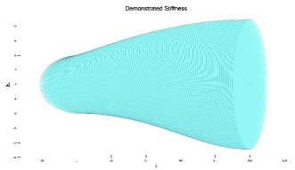
Figure 2: The demonstrated stiffness ellipsoids are visualized at different time steps.

First assume that the damping coefficient is known and a constant as $\boldsymbol{D}_{t}=50$. The comparisons between the proposed algorithm and the method outlined in [17], as well as the convex optimization introduced in [16] are presented and analyzed. The stiffness in equation 4 is estimated by solving the following convex optimization problem.

$$\mathrm{minimize}\;\;||\boldsymbol{K}\boldsymbol{X}-\boldsymbol{Y}||_{2},\;\;\mathrm{subject\;to}\;\boldsymbol{K}\succeq\boldsymbol{0},$$ (43)

where $\boldsymbol{K}\succeq\boldsymbol{0}$ denotes that $\boldsymbol{K}$ is a positive semi-definite matrix.

The average computation time for the nearest–SPD approximation [17], convex optimization [16], and the proposed algorithm are 0.23, 312, and 0.24 ms per time step, respectively. The results of these algorithms compared with the ground truth are shown in Fig. 3.

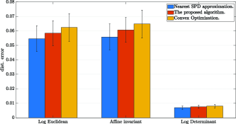
Figure 3: Considering a known constant damping, compare the performance of the estimated stiffness using the proposed algorithm with nearest-SPD approximation and the convex optimization.

It can be seen from Fig. 3 that all the three approaches can acquire accurate estimates of the stiffness. The nearest–SPD approximation [17] produces the lowest error across all three metrics, indicating that it exhibits slightly better performance in estimating stiffness compare with the ground truth. However, it is worth noting that the estimation process involves the use of sliding windows in the simulation, and as the actual stiffness varies within these windows, the ground truth may not be identical to the true value but rather a close approximation.

To get a better consistency with the process of the least squares, changing the original optimization problem to the following formulation when using the convex optimization:

$$\mathrm{minimize}\;\;||\boldsymbol{K}\boldsymbol{X}\boldsymbol{X}^{\mathrm{T}}-\boldsymbol{Y}\boldsymbol{X}^{\mathrm{T}}||_{2},\;\;\mathrm{subject\;to}\;\boldsymbol{K}\succeq\boldsymbol{0},$$ (44)

Then an interesting result is acquired as the estimated stiffness obtained from the proposed algorithm aligns closely with that obtained using the convex optimization method in the majority of cases.

Afterwards, a simulation assumes that the damping coefficient is not precisely known but guess it from $26$ to $58$ which are close to the actual value. The performances of estimating stiffness using the three algorithms compare the ground truth are shown in Fig. 4.

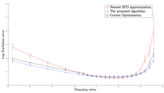
Figure 4: The stiffness estimation results obtained from applying the proposed algorithm with nearest-SPD approximation and the convex optimization method while varying the damping.

Fig. 4 illustrates the performance of the Log-Euclidean error metric, while the other metrics are not shown as they behave similarly when the damping value is altered. The findings indicate that all the approaches are capable of accurately estimating the stiffness, even when different damping values are utilized. However, there are notable distinctions in their performance. The proposed algorithm exhibits greater robustness in estimating the desired stiffness across a range of damping values. In contrast, the nearest-SPD approximation and the convex optimization method display a slightly larger variation in stiffness estimates as the damping changes. Specifically, increasing damping error results in decreased accuracy of estimated stiffness for all these three methods. However, the proposed algorithm shows a slower rate of decrease compare with the other two algorithms making it a more suitable choice for applications where damping is unknown constant.

In practical experiments, it is common for both the stiffness and damping parameters to be unknown and in need of estimation from demonstrations. Assuming the damping is an unknown constant, both the proposed algorithm and the convex optimization approach are used to estimate both the stiffness and damping. To handle the potential variation of damping over time. First, the stiffness and damping are estimated using the sliding windows. Then, the average damping value is calculated based on the estimated value obtained from each window. Subsequently, the stiffness is re-estimated using the calculated average damping. This two-step process allows for more accurate estimation of both the stiffness and damping and satisfies the constant damping assumption. The estimated results are shown in Fig. 5, which demonstrate that even without prior knowledge of the damping, the proposed algorithm and the Convex optimization method can accurately estimate both the stiffness and the damping. Notably, the proposed algorithm demonstrates a distinct advantage in terms of speed, as the two algorithms are implemented twice, making it considerably faster than the Convex optimization approach.

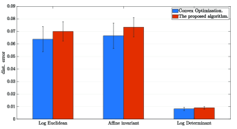
Figure 5: Compare the performance of the estimated stiffness using the proposed algorithm with the convex optimization when assuming that damping is an unknown constant.

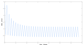
Figure 6: The error between the iterative method and the ground truth. The x-axis represents the number of iterations and the y-axis represents the error.

When assuming that both the stiffness and damping are unknown matrices, and the demonstration behavior satisfies critical damping. The convex optimization method cannot handle this problem since the constraints between stiffness and damping are non-convex. While the proposed algorithm can estimate the stiffness iteratively. To evaluate the iterative method, another self-made dataset is generated by 2-degree-of-freedom mass-spring-damper with the stiffness and damping values that satisfy critical damping. The estimated stiffness obtained using the given damping is considered to be the ground truth and is used for comparison. The Log-Euclidean error between the iterative method and the ground truth is depicted in Figure 6, as the number of iterations increases. The results demonstrate that as the number of iterations increases, the error decreases and converges to a low value. However, the variation when compared to the first estimation is not substantial. This implies that assuming the damping as an unknown constant still results in not bad performance when the demonstrations exhibit critical damping. Therefore, in real experimental scenarios, assuming damping as an unknown constant can lead to accurate estimation of stiffness by utilizing the proposed algorithm when acquiring demonstrations.

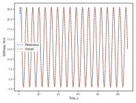
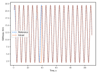
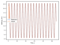
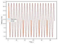
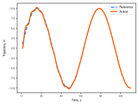
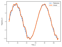
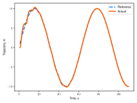
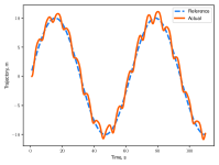
Figure 7: Compare the performance of the proposed algorithm with the original tank-based variable impedance control approach. Real stiffness and trajectory are plotted against reference stiffness and trajectory, respectively, as shown in the top and bottom rows, respectively.

IV-B Simulation on Validating the Novel Tank Based Approach

To evaluate the effectiveness of the proposed novel tank-based variable impedance control approach, a series of simulations were conducted and compared to the original tank-based approach [23]. It is worth noting that variable impedance control aims to achieve the desired interactive rather than precise trajectory tracking. Therefore, in these simulations, the priority was given to maintaining stability by ensuring similarity between the implemented stiffness and predefined stiffness. Once stability was achieved, the focus shifted towards accurately tracking the reference trajectory.

The section presents a reproduction of the simulation conducted in [23], which involves a 1 degree of freedom (dof) system with variable stiffness. The reference trajectory and desired stiffness are defined as:

$$\begin{cases}x^{d}_{t}=10\sin(0.1t),\\ k^{d}_{t}=k_{c}+10\sin(t),\end{cases}$$ (45)

The system is simulated using a mass of 10 Kg and a damping of 1 Ns/m. Since there is no interaction force in this simulation, $\xi$ in equation (25) can be set to $V(\boldsymbol{e},\dot{\boldsymbol{e}},0)/5$. However, setting a tighter condition can improve tracking performance, which is $\xi=V(\boldsymbol{e},\dot{\boldsymbol{e}},0)/10$ in this paper.

Setting $k_{c}=13$ in (45) may not always satisfy the stability conditions proposed by [22], which often require tank-based approaches to ensure stability. However, it is interesting to note that when using the provided stiffness directly, the system remains stable with $k_{c}=13$. On the other hand, if $k_{c}=12$, the system becomes unstable, and the actual trajectory would diverge, indicating the necessity of a tank-based approach to stabilize the system. When the simulation runs for 110 seconds, by using the reference stiffness, the real trajectories of the system are shown in Fig. (6). And the performances of the proposed tank-based approach compare the original tank-based approach [23] to control the system with $k_{c}=13$ and $k_{c}=12$ are shown in Fig. 6.

In the original tank-based approach, stiffness is modified online and, when the tank is empty, it falls back to a constant value of $k_{c}$. The proposed approach also operates online and adjusts the rate of change of stiffness to zero when the tracking error exceeds a certain threshold. In Fig. 6.a, the top plot shows the reference stiffness and actual stiffness, while the bottom plot shows the reference trajectory and actual trajectory when $k_{c}=13$. Similarly, Fig. 6.b shows results for $k_{c}=12$. For comparison, Fig. 6.c and Fig. 6.d show the same plots as in Fig. 6.a and 6.b, but using the original tank-based approach instead of the proposed algorithm. The simulation considers a linear scalar system with varying stiffness, where the only factor affecting performance is stiffness. Comparing results of the proposed algorithm to the original tank-based approach, it can be observed that the actual stiffness is more similar to the reference stiffness when using the proposed algorithm. Moreover, the real trajectory also exhibits greater similarity to the reference trajectory with the proposed algorithm.

V Conclusions and Future Work

In this paper, a framework is proposed for variable impedance control learning from demonstration. The performance of the proposed framework is investigated using the demonstrated examples in a manually designed dateset. The experimental results confirm the effectiveness of the proposed method.

References

- [1] Y. Zimmermann et al., ”Human–Robot Attachment System for Exoskeletons: Design and Performance Analysis,” IEEE Transactions on Robotics, Early Access.
- [2] A.C. Dometios and C.S. Tzafestas, ”Interaction Control of a Robotic Manipulator With the Surface of Deformable Object,” IEEE Transactions on Robotics, vol. 39, no. 2, pp. 1321-1340, April 2023.
- [3] H. Ravichandar, A.S. Polydoros, and S. Chernova, ”Recent Advances in Robot Learning from Demonstration,” Annual Review of Control Robotics and Autonomous Systems, vol. 3, no. 1, pp. 297-330, 2020.
- [4] L. Biagiotti, R. Meattini, D. Chiaravalli, G. Palli and C. Melchiorri, ”Robot Programming by Demonstration: Trajectory Learning Enhanced by sEMG-Based User Hand Stiffness Estimation,” IEEE Transactions on Robotics, Early Access.
- [5] Y. Zhang, L. Cheng, H. Li and R. Cao, ”Learning Accurate and Stable Point-to-Point Motions: A Dynamic System Approach,” IEEE Robotics and Automation Letters, vol. 7, no. 2, pp. 1510-1517, 2022.
- [6] C. Zeng, Y. Li, J. Guo, Z. Huang, N. Wang and C. Yang, ”A Unified Parametric Representation for Robotic Compliant Skills With Adaptation of Impedance and Force,” IEEE/ASME Transactions on Mechatronics, vol. 27, no. 2, pp. 623-633, 2022.
- [7] T.K. Best, C.G. Welker, E.J. Rouse and R.D. Gregg, ”Data-Driven Variable Impedance Control of a Powered Knee–Ankle Prosthesis for Adaptive Speed and Incline Walking,” IEEE Transactions on Robotics, Early Access.
- [8] E. Burdet, R. Osu, D. Franklin, T.E. Milner, and M. Kawato, ”The central nervous system stabilizes unstable dynamics by learning optimal impedance,” Nature, vol. 414, pp. 446–449, 2001.
- [9] C. Yang, G. Ganesh, S. Haddadin, S. Parusel, A. Albu-Schaeffer and E. Burdet, ”Human-Like Adaptation of Force and Impedance in Stable and Unstable Interactions,” IEEE Transactions on Robotics, vol. 27, no. 5, pp. 918-930, 2011.
- [10] Y. Michel, R. Rahal, C. Pacchierotti, P. R. Giordano and D. Lee, ”Bilateral Teleoperation With Adaptive Impedance Control for Contact Tasks,” IEEE Robotics and Automation Letters, vol. 6, no. 3, pp. 5429-5436, 2021.
- [11] Y. Lin, Z. Chen and B. Yao, ”Unified Motion/Force/Impedance Control for Manipulators in Unknown Contact Environments Based on Robust Model-Reaching Approach,” IEEE/ASME Transactions on Mechatronics, vol. 26, no. 4, pp. 1905-1913, 2021.
- [12] R. Martín-Martín, M. A. Lee, R. Gardner, S. Savarese, J. Bohg and A. Garg, ”Variable Impedance Control in End-Effector Space: An Action Space for Reinforcement Learning in Contact-Rich Tasks,” in Proceedings ofIEEE/RSJ International Conference on Intelligent Robots and Systems, Macau, China, 2019, pp. 1010-1017.
- [13] B. Jonas, S. Freek, T. Evangelos, and S. Stefan, ”Learning variable impedance control,” The International Journal of Robotics Research, vol. 30, no. 7, pp. 820-833, 2011.
- [14] Y. Zhu, Q. Wu, B. Chen and Z. Zhao, ”Design and Voluntary Control of Variable Stiffness Exoskeleton Based on sEMG Driven Model,” IEEE Robotics and Automation Letters, vol. 7, no. 2, pp. 5787-5794, 2022.
- [15] J. Arnold and H. Lee, ”Variable Impedance Control for pHRI: Impact on Stability, Agility, and Human Effort in Controlling a Wearable Ankle Robot,” IEEE Robotics and Automation Letters, vol. 6, no. 2, pp. 2429-2436, 2021.
- [16] L. Rozo, S. Calinon, D. G. Caldwell, P. Jimenez, and C. Torras, ”Learning physical collaborative robot behaviors from human demonstrations,” IEEE Transactions on Robotics, vol. 32, no. 3, pp. 513-527, 2016.
- [17] F.J. Abu-Dakka, L. Rozo, and D. Caldwell, ”Force-based variable impedance learning for robotic manipulation,” Robotics and Autonomous Systems, vol. 109, pp. 156-167, 2018.
- [18] C. Zeng, C. Yang, H. Cheng, Y. Li, and S.L. Dai, ”Simultaneously encoding movement and sEMG-based stiffness for robotic skill learning,” IEEE Transactions on Industrial Informatics, vol. 17, no. 2, pp. 1244–1252, 2021.
- [19] Y. Zhao, K. Qian, S. Bo, Z. Zhang, Z. Li, G. Li, A.A. Dehghani-Sanij, and S.Q. Xie, ”Adaptive Cooperative Control Strategy for a Wrist Exoskeleton Using Model-Based Joint Impedance Estimation,” IEEE/ASME Transactions on Mechatronics, vol. 28, no. 2, pp. 748-757, 2023.
- [20] Y. Zhang, L. Cheng, R. Cao, H. Li, and C. Yang, ”A neural network based framework for variable impedance skills learning from demonstrations,” Robotics and Autonomous Systems, vol. 160, 2023.
- [21] M. Bogdanovic, M. Khadiv and L. Righetti, ”Learning Variable Impedance Control for Contact Sensitive Tasks,” IEEE Robotics and Automation Letters, vol. 5, no. 4, pp. 6129-6136, Oct. 2020.
- [22] K. Kronander and A. Billard, ”Stability Considerations for Variable Impedance Control,” IEEE Transactions on Robotics, vol. 32, no. 5, pp. 1298-1305, 2016.
- [23] F. Ferraguti, C. Secchi, and C. Fantuzzi, “A tank-based approach to impedance control with variable stiffness,” in Proceedings of IEEE International Conference on Robotics and Automation, Karlsruhe, Germany, 2013, pp. 4948-4953.
- [24] F.E. Tosun and V. Patoglu, ”Necessary and sufficient conditions for the passivity of impedance rendering with velocity-sourced series elastic actuation,” IEEE Transactions on Robotics, vol. 36, no. 3, pp. 757-772, 2020.
- [25] C. Bishop, ”Pattern Recognition and Machine Learning,” Information Science and Statistics, New York: Springer, Vo. 1, Ch. 6, pp. 291-294, 2006.
- [26] O. Khatib, ”A unified approach for motion and force control of robot manipulators: The operational space formulation,” IEEE Journal on Robotics and Automation, vol. 3, no. 1, pp. 43-53, 1987.
- [27] F.A. Mussa-Ivaldi, N. Hogan, and E. Bizzi, ”Neural, mechanical, and geometric factors subserving arm posture in humans,” The Journal of Neuroscience, vol. 5, no. 10, pp. 2732-2743, 1987.
- [28] S. Jayasumana, R. Hartley, M. Salzmann, H. Li, and M. Harandi, ”Kernel methods on riemannian manifolds with gaussian rbf kernels,” IEEE Transactions on Pattern Analysis and Machine Intelligence, vol. 37, no. 12, pp. 2464-2477, 2015.
- [29] S. Jayasumana, R. Hartley, M. Salzmann, H. Li, and M. Harandi, ”Kernel methods on riemannian manifolds with gaussian rbf kernels,” IEEE Transactions on Pattern Analysis and Machine Intelligence, vol. 37, no. 12, pp. 2464-2477, 2015.
- [30] A.J. Ijspeert, J. Nakanishi, H. Hoffmann, P. Pastor, and S. Schaal, ”Dynamical movement primitives: Learning attractor models for motor behaviors,” Neural Computation, vol. 25, no. 2, pp. 328-373, 2013.