Traversing Between Modes in Function Space for Fast Ensembling

Abstract

Deep ensemble is a simple yet powerful way to improve the performance of deep neural networks. Under this motivation, recent works on mode connectivity have shown that parameters of ensembles are connected by low-loss subspaces, and one can efficiently collect ensemble parameters in those subspaces. While this provides a way to efficiently train ensembles, for inference, multiple forward passes should still be executed using all the ensemble parameters, which often becomes a serious bottleneck for real-world deployment. In this work, we propose a novel framework to reduce such costs. Given a low-loss subspace connecting two modes of a neural network, we build an additional neural network that predicts the output of the original neural network evaluated at a certain point in the low-loss subspace. The additional neural network, which we call a “bridge”, is a lightweight network that takes minimal features from the original network and predicts outputs for the low-loss subspace without forward passes through the original network. We empirically demonstrate that we can indeed train such bridge networks and significantly reduce inference costs with the help of bridge networks.

1 Introduction

Deep Ensemble (de) (Lakshminarayanan et al., 2017) is a simple algorithm to improve both the predictive accuracy and the uncertainty calibration of deep neural networks, where a neural network is trained multiple times using the same data but with different random seeds. Due to this randomness, the parameters obtained from the multiple training runs reach different local optima, called modes, on the loss surface (Fort et al., 2019). These parameters represent a set of various functions that serve as an effective approximation for Bayesian Model Averaging (bma) (Wilson & Izmailov, 2020).

An apparent drawback of de is that it requires multiple training runs. This cost can be huge especially for large-scale settings for which parallel training is not feasible. Garipov et al. (2018) and Draxler et al. (2018) showed that the modes in the loss surface of a deep neural network are connected by relatively simple low-dimensional subspaces where every parameter in those subspaces retains low training error, and the parameters along those subspaces are good candidates for ensembling. Based on this observation, Garipov et al. (2018) and Huang et al. (2017) proposed algorithms to quickly construct deep ensembles without having to run multiple independent training runs.

While the fast ensembling methods based on mode connectivity reduce training costs, they do not address another important drawback of de; the inference cost. One should still execute multiple forward passes using all the parameters collected for the ensemble, and this cost often becomes critical for a real-world scenario, where the training is done in a resource-abundant setting with plenty of computation time, but for the deployment, the inference should be done in a resource-limited environment. For such settings, reducing the inference cost is much more important than reducing the training cost.

In this paper, we propose a novel approach to scale up de by reducing the inference cost. We start from an assumption; if two modes in an ensemble are connected by a simple subspace, we can predict the outputs corresponding to the parameters in the subspace using only the outputs computed from the modes. In other words, we can predict the outputs evaluated in the subspace without having to forward the actual parameters in the subspace through the network. If this is indeed possible, for instance, given two modes, we can approximate an ensemble of three models consisting of parameters collected from three different locations (one from the subspace connecting two modes, and two from each mode) with only two forward passes and a small auxiliary forward pass.

We show that we can actually implement this idea using an additional lightweight network whose inference cost is relatively low compared to that of the original neural network. This additional network, what we call a “bridge network”, takes some features from the original neural network (e.g., features from the penultimate layer) and directly predicts the outputs computed from the connecting subspace. In other words, the bridge network lets us travel between modes in the function space.

We present two types of bridge networks depending on the number of modes involved in prediction, network architectures for bridge networks, and training procedures. Through empirical validation on various image classification benchmarks, we show that (1) bridge networks can predict outputs of connecting subspaces quite accurately with minimal computation cost, and (2) des augmented with bridge networks can significantly reduce inference costs without big sacrifice in performance.

Figure 1: Ensembles with a Bezier curve (left), a type I bridge network (center), and a type II bridge network (right).

2 Preliminaries

2.1 Problem setup

In this paper, we discuss the $K$-way classification problem taking $D$-dimensional inputs. A classifier is constructed with a deep neural network $f_{{\boldsymbol{\theta}}}:\mathbb{R}^{D}\to\mathbb{R}^{K}$ which is decomposed into a feature extractor $f^{(\text{ft})}_{\boldsymbol{\phi}}:\mathbb{R}^{D}\to\mathbb{R}^{D_{\text{ft}}}$ and a classifier $f^{(\text{cls})}_{{\boldsymbol{\psi}}}:\mathbb{R}^{D_{\text{ft}}}\to\mathbb{R}^{K}$, i.e., $f_{{\boldsymbol{\theta}}}(\boldsymbol{x})=f^{(\text{cls})}_{\boldsymbol{\psi}}\circ f^{(\text{ft})}_{\boldsymbol{\phi}}(\boldsymbol{x})$. Here, ${\boldsymbol{\phi}}\in\boldsymbol{\Phi}$ and ${\boldsymbol{\psi}}\in\boldsymbol{\Psi}$ denote the parameters for the feature extractor and classifier, respectively, ${\boldsymbol{\theta}}=({\boldsymbol{\phi}},{\boldsymbol{\psi}})\in\boldsymbol{\Theta}$, and $D_{\text{ft}}$ is the dimension of the feature. An output from the classifier corresponds to a class probability vector.

2.2 Finding low-loss subspaces

While there are few low-loss subspaces that are known to connect modes of deep neural networks, in this paper, we focus on Bezier curves as suggested in (Garipov et al., 2018). Let ${\boldsymbol{\theta}}_{i}$ and ${\boldsymbol{\theta}}_{j}$ be two parameters (usually corresponding to modes) of a neural network. The quadratic Bezier curve between them is defined as

$$\Big{\{}(1-r)^{2}{\boldsymbol{\theta}}_{i}+2r(1-r){\boldsymbol{\theta}}^{(\text{be})}_{i,j}+r^{2}{\boldsymbol{\theta}}_{j}\,|\,r\in[0,1]\Big{\}},$$ (1)

where ${\boldsymbol{\theta}}^{(\text{be})}_{i,j}$ is a pin-point parameter characterizing the curve. Based on this curve paramerization, a low-loss subspace connecting $({\boldsymbol{\theta}}_{i},{\boldsymbol{\theta}}_{j})$ is found by minimizing the following loss w.r.t. ${\boldsymbol{\theta}}^{(\text{be})}_{i,j}$,

$$\int_{0}^{1}{\mathcal{L}}\Big{(}{\boldsymbol{\theta}}^{(\text{be})}_{i,j}(r)\Big{)}\mathrm{d}r,$$ (2)

where ${\boldsymbol{\theta}}^{(\text{be})}_{i,j}(r)$ denotes the parameter at the position $r$ of the curve,

$${\boldsymbol{\theta}}^{(\text{be})}_{i,j}(r)=(1-r)^{2}{\boldsymbol{\theta}}_{i}+2r(1-r){\boldsymbol{\theta}}^{(\text{be})}_{i,j}+r^{2}{\boldsymbol{\theta}}_{j},$$ (3)

and ${\mathcal{L}}:\boldsymbol{\Theta}\to\mathbb{R}$ is the loss function evaluating parameters (e.g., cross entropy). Since the integration above is usually intractable, we instead minimize the stochastic approximation:

$$\mathbb{E}_{r\sim{\mathcal{U}}(0,1)}\left[{\mathcal{L}}\left({\boldsymbol{\theta}}^{(\text{be})}_{i,j}(r)\right)\right],$$ (4)

where ${\mathcal{U}}(0,1)$ is the uniform distribution on $[0,1]$. For a more detailed procedure of Bezier curve training, please refer to Garipov et al. (2018).

2.3 Ensembles with Bezier curves

Let $\{{\boldsymbol{\theta}}_{1},\dots,{\boldsymbol{\theta}}_{m}\}$ be a set of parameters independently trained as a deep ensemble. Then, for each pair $({\boldsymbol{\theta}}_{i},{\boldsymbol{\theta}}_{j})$, we can construct a low-loss Bezier curve. Since all of the parameters along those Bezier curves achieve low loss, we can add them to the ensemble for improved performance. For instance, choosing $r=0.5$, we can collect ${\boldsymbol{\theta}}^{(\text{be})}_{i,j}(0.5)$ for all $(i,j)$ pairs, and construct an ensembled predictor as

$$\frac{1}{m+\binom{m}{2}}\bigg{(}\sum_{i=1}^{m}f_{{\boldsymbol{\theta}}_{i}}(\boldsymbol{x})+\sum_{i<j}f_{{\boldsymbol{\theta}}^{(\text{be})}_{i,j}(0.5)}(\boldsymbol{x})\bigg{)}.$$ (5)

While this strategy provide an effective way to increase the number of ensemble members, for inference, an additional ${\mathcal{O}}(m^{2})$ number of forward passes are required. Our primary goal in this paper is to reduce this additional cost by bypassing the direct forward passes with ${\boldsymbol{\theta}}^{(\text{be})}_{i,j}(r)$.

3 Main contribution

In this section, we present a novel method that directly predicts the outputs of neural networks evaluated at parameters on Bezier curves without actual forward passes with them.

3.1 Bridge networks

Let us first recall our key assumption stated in the introduction; if two modes in an ensemble are connected by a simple low-loss subspace (Bezier curve), then we can predict the outputs corresponding to the parameters on the subspace using only the information obtained from the modes. The intuition behind this assumption is that, since the parameters are connected with a simple curve, the corresponding outputs may also be connected via a relatively simple mapping, which is far less complex than the original neural network. If such mapping exists, we may learn them via a lightweight neural network.

More specifically, let $\boldsymbol{z}_{i}:=f^{(\text{ft})}_{{\boldsymbol{\phi}}_{i}}(\boldsymbol{x})$ and $\boldsymbol{v}_{i}:=f_{{\boldsymbol{\theta}}_{i}}(\boldsymbol{x})=f^{(\text{cls})}_{{\boldsymbol{\psi}}_{i}}(\boldsymbol{z}_{i})$ for $i\in\{1,\dots,m\}$. Let $\boldsymbol{v}_{i,j}(r):=f_{{\boldsymbol{\theta}}^{(\text{be})}_{i,j}(r)}(\boldsymbol{x})$. In order to use $\boldsymbol{v}_{i,j}(r)$ with $\boldsymbol{v}_{i}$ to get an ensemble, we should forward $\boldsymbol{x}$ through $f_{{\boldsymbol{\theta}}^{(\text{be})}_{i,j}(r)}$, starting from the bottom layer. Instead, we reuse $\boldsymbol{z}_{i}$ to predict $\boldsymbol{v}_{i,j}(r)$ with a lightweight neural network. We call such a lightweight neural network a “bridge network”, since it allows us to move directly from $\boldsymbol{v}_{i}$ to $\boldsymbol{v}_{i,j}(r)$ in the function space, not through the actual parameter space. A bridge network is usually constructed with a Convolutional Neural Network (cnn) whose inference cost is much lower than that of $f_{{\boldsymbol{\theta}}_{i}}$.

From the following, we introduce two types of bridge networks depending on the number of modes involved in the computation. Figure 1 presents a schematic diagram that compares forward passes of ensembles with/without bridge networks.

Type I bridge networks

A type I bridge network $h^{(r)}_{i,j}$ takes a feature $\boldsymbol{z}_{i}$ from one mode and predicts $\boldsymbol{v}_{i,j}(r)$ as

$$\boldsymbol{v}_{i,j}(r)\approx\tilde{\boldsymbol{v}}_{i,j}(r)=h^{(r)}_{i,j}(\boldsymbol{z}_{i}).$$ (6)

A type I bridge network can be constructed between any pair of connected modes $({\boldsymbol{\theta}}_{i},{\boldsymbol{\theta}}_{j})$ and an ensembled prediction for specific mode ${\boldsymbol{\theta}}_{i}$ with its Bezier parameter ${\boldsymbol{\theta}}^{(\text{be})}_{i,j}$ can be approximated as

$$\frac{1}{2}\bigg{(}\boldsymbol{v}_{i}+h^{(r)}_{i,j}(\boldsymbol{z}_{i})\bigg{)},$$ (7)

whose inference cost is nearly identical to that of $\boldsymbol{v}_{i}$ (nearly a single forward pass). One can also connect ${\boldsymbol{\theta}}_{i}$ with multiple modes $\{{\boldsymbol{\theta}}_{j_{1}},\dots,{\boldsymbol{\theta}}_{j_{k}}\}$, learn bridge networks between $(i,j_{1}),\dots,(i,j_{k})$, and construct an ensemble

$$\frac{1}{1+k}\bigg{(}\boldsymbol{v}_{i}+\sum_{j=1}^{k}h^{(r)}_{i,j_{k}}(\boldsymbol{z}_{i})\bigg{)}.$$ (8)

Still, since the costs for $h^{(r)}_{i,j_{k}}$s are much lower than $\boldsymbol{v}_{i}$, the inference cost does not increase significantly.

Type II bridge networks

A type II bridge network between $({\boldsymbol{\theta}}_{i},{\boldsymbol{\theta}}_{j})$ takes two features $(\boldsymbol{z}_{i},\boldsymbol{z}_{j})$ to predict $\boldsymbol{v}_{i,j}(r)$.

$$\boldsymbol{v}_{i,j}(r)\approx\tilde{\boldsymbol{v}}_{i,j}(r)=H^{(r)}_{i,j}(\boldsymbol{z}_{i},\boldsymbol{z}_{j}).$$ (9)

An ensembled prediction with the type II bridge network is then constructed as

$$\frac{1}{3}\bigg{(}\boldsymbol{v}_{i}+\boldsymbol{v}_{j}+H^{(r)}_{i,j}(\boldsymbol{z}_{i},\boldsymbol{z}_{j})\bigg{)},$$ (10)

where we construct an ensemble of three models with effectively two forward passes (for $\boldsymbol{v}_{i}$ and $\boldsymbol{v}_{j}$). Similar to the type I bridge networks, we may construct multiple bridges between modes and use them together for an ensemble.

3.2 Learning bridge networks

Fixing a position $r$ on Bezier curves

In the definition of the bridge networks above, we fixed the value $r$. In principle, we may parameterize the bridge networks to take $r$ as an additional input to predict $\boldsymbol{v}_{i,j}(r)$ for any $r\in[0,1]$, but we found this to be ineffective due to the difficulty of learning all the outputs corresponding to arbitrary $r$ values. Moreover, as we empirically observed in Figure 2, the ensemble with Bezier parameters is most effective with $r=0.5$, and adding additional parameters evaluated at different $r$ values does not significantly improve the performance. To this end, we fix $r=0.5$ and aim to learn bridge networks predicting $\boldsymbol{v}_{i,j}(0.5)$ throughout the paper. See § B.1 for more detailed inspection.

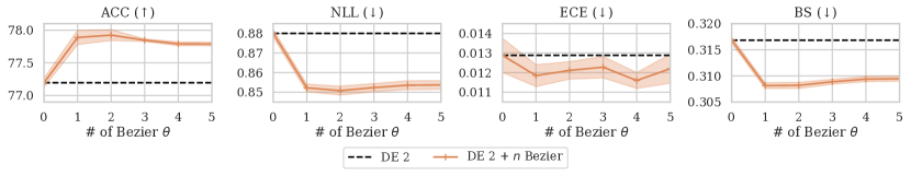
Figure 2: Performance of an ensemble of two modes and a parameter from the Bezier curve connecting them, evaluated for ResNet-50 on ImageNet. Here, $r\in(0,1)$ denotes a position on the curve. (Top) Ensemble performances when one member from the Bezier curve $r$ is added to de-2. (Bottom) Ensemble performances when members are sequentially added to de-2 from a Bezier curve. For accuracy, the higher is better, and for NLL, ECE and BS, the lower is better.

Training procedure

Let $\{{\boldsymbol{\theta}}_{1},\dots,{\boldsymbol{\theta}}_{m}\}$ be a set of parameters in an ensemble. Given a set of Bezier parameters $\{{\boldsymbol{\theta}}^{(\text{be})}_{i,j}\}$ connecting them, we learn bridge networks (either type I or II) for each Bezier curve. The training procedure is straightforward. We minimize the Kullback-Leibler divergence between the actual output from the Bezier parameters and the prediction made from the bridge network. It makes the bridge network imitate the original function defined by the Bezier parameters in the same manner as a conventional knowledge distillation (Hinton et al., 2015).

Further, we apply the mixup (Zhang et al., 2018) method to explore more diverse responses, preventing the bridge from learning to just copy the outputs of the base model. Refer to § A.1 for the detailed training procedure.

4 Related Works

Mode connectivity

The geometric properties of deep neural networks’ loss surfaces have been studied, and one notable property is the mode connectivity (Garipov et al., 2018; Draxler et al., 2018); there exists a simple path between modes of a neural network on which the network retains low training error along that path. From this, fast ensembling methods that collect ensemble members on the mode-connecting-paths have been proposed (Huang et al., 2017; Garipov et al., 2018). Extending this idea, Izmailov et al. (2020) approximated the posteriors of Bayesian neural nets via the low-loss subspace and used them for bma. Wortsman et al. (2021) also presented a method for further improving performance by ensembling over the subspaces.

Efficient ensembling

Despite the superior performance of de (Lakshminarayanan et al., 2017; Ovadia et al., 2019), it suffers from additional computation costs for both the training and the inference. There have been several works that reduce the computational burden in training by collecting ensemble members efficiently (Huang et al., 2017; Garipov et al., 2018; Benton et al., 2021), but they did not consider inference costs that arose from multiple forward passes. On the other hand, there also exist inference-efficient ensembling methods by sharing parameters (Wen et al., 2019; Dusenberry et al., 2020) or sharing representations (Lee et al., 2015; Siqueira et al., 2018; Antorán et al., 2020; Havasi et al., 2021). In particular, Antorán et al. (2020) and Havasi et al. (2021) presented the methods to obtain an ensemble prediction by a single forward pass. Nevertheless, these methods do not scale well for complex large-scale datasets or require large network capacity.

5 Experiments

In this section, we are going to answer the following three big questions:

1. Do bridge networks really learn to predict the outputs of a function from the Bezier curves?

2. How much ensemble gain we obtain via bridge networks with lower computational complexity?

3. How many bridge networks do we have to make in order to achieve certain ensemble performances?

We answer them in §§ 5.2, 5.3 and 5.4 with empirical validation.

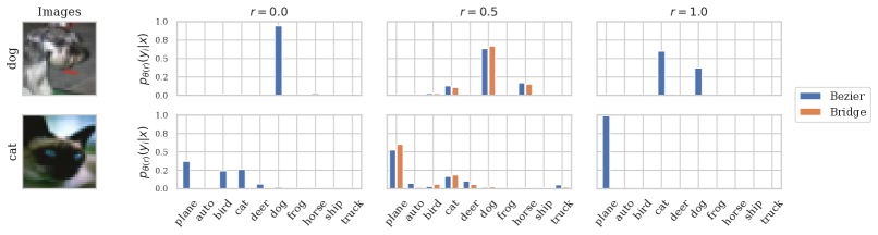
Figure 3: Bar plots in the third column show the class probability outputs of the bridge network (orange) and the base model with the Bezier parameters (blue) for given images displayed in the first column. We also depict the predicted outputs from the base model with ${\boldsymbol{\theta}}_{1}$ and ${\boldsymbol{\theta}}_{2}$ in the second and fourth columns, respectively. Additional results are in § B.6.

Table 1: $R^{2}$ scores and KL divergence values quantify how similar the following models to the target function defined with Bezier parameters ${\boldsymbol{\theta}}^{(\text{be})}_{1,2}(0.5)$ are in output probabilities; ‘Match Type I/II Bridge’, ‘Other Type I/II Bridge’, and ‘Other Bezier’. Refer to § 5.2 for a detailed description of each model. All values are measured on the test split of each dataset.

Dataset	CIFAR-10		CIFAR-100		Tiny ImageNet		ImageNet
Model	$R^{2}$ ($\uparrow$)	KL ($\downarrow$)	$R^{2}$ ($\uparrow$)	KL ($\downarrow$)	$R^{2}$ ($\uparrow$)	KL ($\downarrow$)	$R^{2}$ ($\uparrow$)	KL ($\downarrow$)
Match type I bridge	0.916 $\pm{\,0.003}$	0.131 $\pm{\,0.005}$	0.805 $\pm{\,0.006}$	0.388 $\pm{\,0.011}$	0.751 $\pm{\,0.498}$	0.498 $\pm{\,0.015}$	0.906 $\pm{\,0.001}$	0.229 $\pm{\,0.002}$
Other type I bridge	0.908 $\pm{\,0.002}$	0.148 $\pm{\,0.004}$	0.780 $\pm{\,0.005}$	0.450 $\pm{\,0.010}$	0.719 $\pm{\,0.588}$	0.588 $\pm{\,0.045}$	0.894 $\pm{\,0.001}$	0.260 $\pm{\,0.004}$
Match type II bridge	0.930 $\pm{\,0.002}$	0.108 $\pm{\,0.003}$	0.837 $\pm{\,0.002}$	0.318 $\pm{\,0.004}$	0.767 $\pm{\,0.004}$	0.459 $\pm{\,0.009}$	0.920 $\pm{\,0.001}$	0.191 $\pm{\,0.003}$
Other type II bridge	0.911 $\pm{\,0.002}$	0.144 $\pm{\,0.003}$	0.794 $\pm{\,0.003}$	0.425 $\pm{\,0.006}$	0.720 $\pm{\,0.008}$	0.573 $\pm{\,0.011}$	0.898 $\pm{\,0.000}$	0.241 $\pm{\,0.002}$
Other Bezier	0.870 $\pm{\,0.004}$	0.229 $\pm{\,0.007}$	0.734 $\pm{\,0.002}$	0.586 $\pm{\,0.002}$	0.655 $\pm{\,0.701}$	0.701 $\pm{\,0.011}$	0.874 $\pm{\,0.002}$	0.323 $\pm{\,0.004}$

5.1 Setup

Datasets and networks

We evaluate the proposed bridge networks on various image classification benchmarks, including CIFAR-10, CIFAR-100, Tiny ImageNet, and ImageNet datasets. Throughout the experiments, we use the family of residual networks (ResNet; He et al., 2016) as a base model: ResNet-32$\times$2 for CIFAR-10, ResNet-32$\times$4 for CIFAR-100, ResNet-34 for Tiny ImageNet and ResNet-50 for ImageNet, where $\times$2 and $\times$4 denotes the multiplier of the number of channels for convolutional layers. The base models for CIFAR datasets have fewer parameters than the (Tiny) ImageNet base models, which have different settings. We construct bridge networks with cnns with a residual path whose inference costs are relatively low compared to those of ResNet base models. For detailed training settings, including bridge network architectures or hyperparameter settings, please refer to § A.4.

By changing the channel size of the convolutional layers in the bridge network, we can balance the trade-off between performance gains with computational costs. We check this trade-off in § B.2. We refer to a bridge network with less than 10% of floating-point operations (FLOPs) compared to the base model as Bridge${}_{\text{sm}}$(small bridge), and a bridge with more than 15% as Bridge${}_{\text{md}}$(medium bridge).

Efficiency metrics

We choose FLOPs and the number of parameters (#Params) for efficiency evaluation as these metrics are commonly used to consider the efficiency (Dehghani et al., 2021). Because FLOPs and #Params of the base model are different for each dataset, we report the relative FLOPs and the relative #Params with respect to the corresponding base model instead for better comparison.

Uncertainty metrics

As suggested by Ashukha et al. (2020), along with the classification accuracy (ACC), we report the calibrated versions of Negative Log-likelihood (NLL), Expected Calibration Error (ECE), and Brier Score (BS) as metrics for uncertainty evaluation. We also measure the Deep Ensemble Equivalent (DEE) score proposed in Ashukha et al. (2020), which shows the relative performance for DE in terms of NLL and roughly be interpreted as effective number of models for an ensemble. See § A.5 for more details.

5.2 Correspondence between bridges and Beziers

Figure 3 visualizes the outputs of the bridge network $H_{1,2}^{(0.5)}$ which predicts the logits from ${\boldsymbol{\theta}}^{(\text{be})}_{1,2}(0.5)$. To be more specific, we visualize the predicted logits from ${\boldsymbol{\theta}}_{1}$, ${\boldsymbol{\theta}}_{2}$, ${\boldsymbol{\theta}}^{(\text{be})}_{1,2}(0.5)$, and the bridge network $H_{1,2}^{(0.5)}$, for two test examples of CIFAR-10. Indeed, the bridge network predicts well the logits from the Bezier curve. § B.6 provides additional examples that further verify this.

To assess the quality of the prediction of bridge networks, we use a set of ensemble parameters $\{{\boldsymbol{\theta}}_{1},{\boldsymbol{\theta}}_{2},\dots,{\boldsymbol{\theta}}_{m}\}$ and Bezier curves between them. If the bridge network $H_{1,2}^{(0.5)}$ predicts $\boldsymbol{v}_{1,2}(0.5)$ well compared to the other baselines, we can confirm that there exists the correspondence between the bridge network and the Bezier curve. To this end, we measure the $R^{2}$ score and Kullback-Leibler divergence (KL) which quantify how similar outputs of the following baselines to that of the target function $f_{{\boldsymbol{\theta}}^{(\text{be})}_{1,2}(0.5)}$; (1) ‘Match type I/II bridge’ denote the bridge network imitating the function of ${\boldsymbol{\theta}}^{(\text{be})}_{1,2}(0.5)$, (2) ‘Other type I/II bridge’ denote the bridge network imitating the function of ${\boldsymbol{\theta}}^{(\text{be})}_{i,j}(0.5)$ for some $(i,j)\neq(1,2)$, and (3) ‘Other Bezier’ denotes the base model with the parameters ${\boldsymbol{\theta}}^{(\text{be})}_{i,j}(0.5)$ for some $(i,j)\neq(1,2)$.

Table 1 summarizes the results. Compared to the baselines (i.e., ‘Other type I/II bridge’ and ‘Other Bezier’), the bridge networks produce more similar outputs to the target outputs. The $R^{2}$ values between the predictions and targets are significantly higher than those from the wrong targets, demonstrating that the bridge predictions indeed are approximating our target outputs of interest.

Table 2: Performance improvement of the ensemble by adding type I bridges to the single base ResNet model on Tiny ImageNet and ImageNet datasets. FLOPs, #Params, and DEE metrics are measured with respect to the single base model. Bridge${}_{\text{sm}}$ and Bridge${}_{\text{md}}$ denote the small and the medium versions of the bridge network based on their FLOPs.

Tiny ImageNet
Model	FLOPs ($\downarrow$)	#Params ($\downarrow$)	ACC ($\uparrow$)	NLL ($\downarrow$)	ECE ($\downarrow$)	DEE ($\uparrow$)
ResNet (de-1)	$\times$ 1.000	$\times$ 1.000	62.66 $\pm{\,0.23}$	1.683 $\pm{\,0.009}$	0.050 $\pm{\,0.004}$	1.000
+ 1 Bridge${}_{\text{sm}}$	$\times$ 1.050	$\times$ 1.057	64.58 $\pm{\,0.17}$	1.478 $\pm{\,0.006}$	0.025 $\pm{\,0.002}$	2.280 $\pm{\,0.086}$
+ 2 Bridge${}_{\text{sm}}$	$\times$ 1.099	$\times$ 1.114	65.37 $\pm{\,0.13}$	1.421 $\pm{\,0.004}$	0.018 $\pm{\,0.002}$	3.087 $\pm{\,0.118}$
+ 3 Bridge${}_{\text{sm}}$	$\times$ 1.149	$\times$ 1.171	65.82 $\pm{\,0.10}$	1.395 $\pm{\,0.003}$	0.015 $\pm{\,0.001}$	3.680 $\pm{\,0.133}$
+ 1 Bridge${}_{\text{md}}$	$\times$ 1.180	$\times$ 1.206	65.13 $\pm{\,0.12}$	1.446 $\pm{\,0.002}$	0.034 $\pm{\,0.002}$	2.709 $\pm{\,0.049}$
+ 2 Bridge${}_{\text{md}}$	$\times$ 1.359	$\times$ 1.412	66.29 $\pm{\,0.06}$	1.388 $\pm{\,0.004}$	0.025 $\pm{\,0.001}$	3.845 $\pm{\,0.171}$
+ 3 Bridge${}_{\text{md}}$	$\times$ 1.539	$\times$ 1.618	66.76 $\pm{\,0.09}$	1.362 $\pm{\,0.003}$	0.023 $\pm{\,0.001}$	4.708 $\pm{\,0.209}$
de-2	$\times$ 2.000	$\times$ 2.000	65.54 $\pm{\,0.25}$	1.499 $\pm{\,0.007}$	0.029 $\pm{\,0.003}$	2.000
ImageNet
Model	FLOPs ($\downarrow$)	#Params ($\downarrow$)	ACC ($\uparrow$)	NLL ($\downarrow$)	ECE ($\downarrow$)	DEE ($\uparrow$)
ResNet (de-1)	$\times$ 1.000	$\times$ 1.000	75.85 $\pm{\,0.06}$	0.936 $\pm{\,0.003}$	0.019 $\pm{\,0.001}$	1.000
+ 1 Bridge${}_{\text{sm}}$	$\times$ 1.061	$\times$ 1.071	76.46 $\pm{\,0.06}$	0.914 $\pm{\,0.000}$	0.012 $\pm{\,0.001}$	1.418 $\pm{\,0.034}$
+ 2 Bridge${}_{\text{sm}}$	$\times$ 1.123	$\times$ 1.141	76.60 $\pm{\,0.06}$	0.907 $\pm{\,0.000}$	0.012 $\pm{\,0.001}$	1.537 $\pm{\,0.026}$
+ 3 Bridge${}_{\text{sm}}$	$\times$ 1.184	$\times$ 1.212	76.69 $\pm{\,0.04}$	0.905 $\pm{\,0.000}$	0.011 $\pm{\,0.001}$	1.584 $\pm{\,0.021}$
+ 1 Bridge${}_{\text{md}}$	$\times$ 1.194	$\times$ 1.222	77.03 $\pm{\,0.07}$	0.889 $\pm{\,0.001}$	0.013 $\pm{\,0.000}$	1.881 $\pm{\,0.022}$
+ 2 Bridge${}_{\text{md}}$	$\times$ 1.389	$\times$ 1.444	77.37 $\pm{\,0.07}$	0.876 $\pm{\,0.001}$	0.013 $\pm{\,0.001}$	2.341 $\pm{\,0.076}$
+ 3 Bridge${}_{\text{md}}$	$\times$ 1.583	$\times$ 1.665	77.48 $\pm{\,0.03}$	0.870 $\pm{\,0.000}$	0.013 $\pm{\,0.000}$	2.618 $\pm{\,0.062}$
de-2	$\times$ 2.000	$\times$ 2.000	77.12 $\pm{\,0.04}$	0.883 $\pm{\,0.001}$	0.012 $\pm{\,0.001}$	2.000

Figure 4: The cost-performance plots of type I bridges compared to de on Tiny ImageNet and ImageNet datasets. The x-axis denotes the relative FLOPs quantifying the inference cost of the model compared to a single base model, and the y-axis shows the corresponding predictive performance. On the basis of de (black dashed line), the upper left position is preferable in ACC, and the lower left position is preferable in NLL.

5.3 Classification with bridge networks

5.3.1 Type I bridge networks

Single model performances with type I bridge networks

In situations where multiple forward passes are not allowed for inference, we can approximate an ensemble of a single base model and the ones from Bezier curves with type I bridge networks. The results are shown in Table 2. The results show that for Stochastic Gradient Descent (sgd) trained single ResNet model, an ensemble with type I bridge networks improves the performance both in terms of accuracy and uncertainty estimation. Only adding one small type I bridge with $5\sim 6\%$ FLOPs to the base model (ResNet + 1 Bridge${}_{\text{sm}}$) dramatically improves the accuracy and DEE on both datasets. Furthermore, using more FLOPs with a medium type I bridge (ResNet + 1 Bridge${}_{\text{md}}$) gives better performance gains.

Using multiple type I bridge networks

As type I bridge network requires features from only one mode of each curve for inference, we can use multiple type I bridge networks for a single base model without significantly increasing inference cost, as we mentioned at Equation 8. Table 2 reports the performance gain of a single base model with an increasing number of type I bridges. Each bridge approximates the models on different Bezier curves between a single mode and others (i.e., Bezier curves between modes A-B, A-C, and so on where A, B, and C are different modes.), not the models on a single Bezier curve. Adding more bridge networks introduces more diverse outputs to the ensembles. One can see that the performance continuously improves as the number of bridges increases, with low additional inference costs. Figure 4 shows how much type I bridge networks efficiently increase the performances proportional to FLOPs.

5.3.2 Type II bridge networks

Table 3: Performance improvement of the ensemble by adding type II bridges as members to existing DE ensembles on Tiny ImageNet and ImageNet datasets. FLOPs, #Params, and DEE metrics are measured with respect to corresponding DEs. Type II bridges consistently improve the accuracy and uncertainty metrics of the ensemble before saturation. Bridge${}_{\text{sm}}$ and Bridge${}_{\text{md}}$ denote the small and the medium versions of the bridge network based on their FLOPs.

Tiny ImageNet
Model	FLOPs ($\downarrow$)	#Params ($\downarrow$)	ACC ($\uparrow$)	NLL ($\downarrow$)	ECE ($\downarrow$)	DEE ($\uparrow$)
de-4	$\times$ 4.000	$\times$ 4.000	67.50 $\pm{\,0.11}$	1.381 $\pm{\,0.004}$	0.018 $\pm{\,0.001}$	4.000
+ 1 Bridge${}_{\text{sm}}$	$\times$ 4.058	$\times$ 4.067	67.86 $\pm{\,0.05}$	1.334 $\pm{\,0.003}$	0.017 $\pm{\,0.002}$	6.051 $\pm{\,0.181}$
+ 2 Bridge${}_{\text{sm}}$	$\times$ 4.117	$\times$ 4.135	68.12 $\pm{\,0.09}$	1.311 $\pm{\,0.005}$	0.015 $\pm{\,0.001}$	8.174 $\pm{\,0.465}$
+ 4 Bridge${}_{\text{sm}}$	$\times$ 4.234	$\times$ 4.269	68.47 $\pm{\,0.14}$	1.288 $\pm{\,0.004}$	0.015 $\pm{\,0.001}$	10.340 $\pm{\,0.773}$
+ 6 Bridge${}_{\text{sm}}$	$\times$ 4.351	$\times$ 4.404	68.51 $\pm{\,0.10}$	1.278 $\pm{\,0.003}$	0.014 $\pm{\,0.001}$	11.268 $\pm{\,0.871}$
+ 1 Bridge${}_{\text{md}}$	$\times$ 4.198	$\times$ 4.226	68.00 $\pm{\,0.11}$	1.333 $\pm{\,0.003}$	0.019 $\pm{\,0.001}$	6.183 $\pm{\,0.120}$
+ 2 Bridge${}_{\text{md}}$	$\times$ 4.395	$\times$ 4.453	68.33 $\pm{\,0.08}$	1.308 $\pm{\,0.003}$	0.019 $\pm{\,0.001}$	8.489 $\pm{\,0.481}$
+ 4 Bridge${}_{\text{md}}$	$\times$ 4.791	$\times$ 4.906	68.61 $\pm{\,0.05}$	1.281 $\pm{\,0.004}$	0.021 $\pm{\,0.003}$	10.897 $\pm{\,0.800}$
+ 6 Bridge${}_{\text{md}}$	$\times$ 5.186	$\times$ 5.359	68.80 $\pm{\,0.09}$	1.269 $\pm{\,0.003}$	0.021 $\pm{\,0.001}$	12.110 $\pm{\,1.083}$
de-5	$\times$ 5.000	$\times$ 5.000	67.90 $\pm{\,0.14}$	1.354 $\pm{\,0.003}$	0.019 $\pm{\,0.001}$	5.000
ImageNet
Model	FLOPs ($\downarrow$)	#Params ($\downarrow$)	ACC ($\uparrow$)	NLL ($\downarrow$)	ECE ($\downarrow$)	DEE ($\uparrow$)
de-4	$\times$ 4.000	$\times$ 4.000	77.87 $\pm{\,0.04}$	0.851 $\pm{\,0.001}$	0.012 $\pm{\,0.001}$	4.000
+ 1 Bridge${}_{\text{sm}}$	$\times$ 4.086	$\times$ 4.088	77.93 $\pm{\,0.02}$	0.847 $\pm{\,0.000}$	0.012 $\pm{\,0.001}$	4.580 $\pm{\,0.052}$
+ 2 Bridge${}_{\text{sm}}$	$\times$ 4.172	$\times$ 4.176	78.00 $\pm{\,0.04}$	0.846 $\pm{\,0.000}$	0.011 $\pm{\,0.000}$	4.739 $\pm{\,0.052}$
+ 4 Bridge${}_{\text{sm}}$	$\times$ 4.343	$\times$ 4.351	78.10 $\pm{\,0.03}$	0.846 $\pm{\,0.000}$	0.011 $\pm{\,0.001}$	4.768 $\pm{\,0.041}$
+ 6 Bridge${}_{\text{sm}}$	$\times$ 4.515	$\times$ 4.527	78.12 $\pm{\,0.05}$	0.846 $\pm{\,0.001}$	0.011 $\pm{\,0.001}$	4.659 $\pm{\,0.037}$
+ 1 Bridge${}_{\text{md}}$	$\times$ 4.243	$\times$ 4.256	78.14 $\pm{\,0.03}$	0.839 $\pm{\,0.000}$	0.011 $\pm{\,0.001}$	6.123 $\pm{\,0.121}$
+ 2 Bridge${}_{\text{md}}$	$\times$ 4.487	$\times$ 4.512	78.30 $\pm{\,0.05}$	0.833 $\pm{\,0.000}$	0.012 $\pm{\,0.001}$	8.068 $\pm{\,0.144}$
+ 4 Bridge${}_{\text{md}}$	$\times$ 4.973	$\times$ 5.024	78.46 $\pm{\,0.04}$	0.828 $\pm{\,0.000}$	0.012 $\pm{\,0.000}$	9.951 $\pm{\,0.163}$
+ 6 Bridge${}_{\text{md}}$	$\times$ 5.460	$\times$ 5.536	78.56 $\pm{\,0.09}$	0.825 $\pm{\,0.000}$	0.012 $\pm{\,0.001}$	10.760 $\pm{\,0.202}$
de-5	$\times$ 5.000	$\times$ 5.000	78.03 $\pm{\,0.03}$	0.844 $\pm{\,0.001}$	0.012 $\pm{\,0.001}$	5.000

Figure 5: The cost-performance plots of type II bridges compared to de on Tiny ImageNet and ImageNet datasets. The x-axis denotes the relative FLOPs quantifying the inference cost of the model compared to de basis from de-2 to de-7, and the y-axis shows the corresponding predictive performance. On the basis of de (black dashed line), the upper left position is preferable in ACC, and the lower left position is preferable in NLL.

Performance

Table 3 summarizes the classification results comparing de, de with Bezier curves, and de with type II bridge networks. For more experimental results including other datasets, please refer to § B.7. From Table 3, one can see that with only a slight increase in the computational costs, the ensembles with bridge networks achieve almost DEE 2.051 ensemble gain for de-4 case on Tiny ImageNet dataset. This gain is not specific only for de-4; the ensembles with type II bridge networks consistently improved predictive accuracy and uncertainty calibration with a small increase in the inference costs. Figure 5 shows how much our type II bridge network achieves high performance in the perspective of relative FLOPs.

Computational cost

We report FLOPs for inference on Table 3 to indicate how much relative computational costs are required for the competing models. Figure 5 summarizes the tradeoff between FLOPs and performance in various metrics. As one can see from these results, our bridge networks could achieve a remarkable gain in performance, so for some cases, adding bridge ensembles achieved performance gains larger than those might be achieved by adding entire ensemble members. For instance, in Tiny ImageNet experiments, de-4 + 2 bridges were better than de-5. Please refer to § B.7 for the full results including various de sizes and other datasets.

5.4 How many type II bridges are required?

For an ensemble of $m$ parameters, the number of pairs that can be connected by Bezier curves is $\binom{m}{2}$, which grows quadratically with $m$. In the previous experiment, we constructed Bezier curves and bridges for all possible pairs (which explains the large inference costs for Bezier ensembles), but in practice, we found that it is not necessary to use bridge networks for all of those pairs. As an example, we compare the performance of de-4 + bridge ensembles with an increasing number of bridges on Tiny ImageNet and ImageNet datasets. The results are summarized in Table 3. Just one small bridge dramatically increases the performance, and the performance gain gradually saturates as we add more bridges. Notably, only one bridge shows similar or better performance than de-5.

Table 4: Comparison of performance improvement of the efficient methods on Tiny ImageNet dataset. FLOPs, #Params, and DEE metrics are measured with respect to the single ResNet-34.

Tiny ImageNet
Model	FLOPs ($\downarrow$)	#Params ($\downarrow$)	ACC ($\uparrow$)	NLL ($\downarrow$)	ECE ($\downarrow$)	DEE ($\uparrow$)
ResNet (de-1)	$\times$ 1.000	$\times$ 1.000	62.66 $\pm{\,0.23}$	1.683 $\pm{\,0.009}$	0.050 $\pm{\,0.004}$	1.000
+ 1 Bridge${}_{\text{sm}}$	$\times$ 1.050	$\times$ 1.057	64.58 $\pm{\,0.17}$	1.478 $\pm{\,0.006}$	0.025 $\pm{\,0.002}$	2.280 $\pm{\,0.086}$
+ 2 Bridge${}_{\text{sm}}$	$\times$ 1.099	$\times$ 1.114	65.37 $\pm{\,0.13}$	1.421 $\pm{\,0.004}$	0.018 $\pm{\,0.002}$	3.087 $\pm{\,0.118}$
+ 3 Bridge${}_{\text{sm}}$	$\times$ 1.149	$\times$ 1.171	65.82 $\pm{\,0.10}$	1.395 $\pm{\,0.003}$	0.015 $\pm{\,0.001}$	3.680 $\pm{\,0.133}$
de-2	$\times$ 2.000	$\times$ 2.000	65.54 $\pm{\,0.25}$	1.499 $\pm{\,0.007}$	0.029 $\pm{\,0.003}$	2.000
de-3	$\times$ 3.000	$\times$ 3.000	66.65 $\pm{\,0.18}$	1.425 $\pm{\,0.005}$	0.024 $\pm{\,0.002}$	3.000
BE-2	$\times$ 2.000	$\times$ 1.001	61.44 $\pm{\,0.16}$	1.651 $\pm{\,0.006}$	0.014 $\pm{\,0.003}$	1.169 $\pm{\,0.079}$
BE-3	$\times$ 3.000	$\times$ 1.002	62.33 $\pm{\,0.24}$	1.603 $\pm{\,0.014}$	0.015 $\pm{\,0.003}$	1.433 $\pm{\,0.070}$
BE-4	$\times$ 4.000	$\times$ 1.003	62.42 $\pm{\,0.58}$	1.607 $\pm{\,0.020}$	0.015 $\pm{\,0.003}$	1.410 $\pm{\,0.098}$
MIMO ($M=2$)	$\times$ 2.000	$\times$ 3.994	63.47 $\pm{\,0.76}$	1.691 $\pm{\,0.013}$	0.065 $\pm{\,0.000}$	0.983 $\pm{\,0.053}$
ResNet (SWA)	$\times$ 1.000	$\times$ 1.000	64.03 $\pm{\,0.21}$	1.519 $\pm{\,0.010}$	0.030 $\pm{\,0.002}$	1.888 $\pm{\,0.074}$
+ 1 Bridge${}_{\text{sm}}$	$\times$ 1.050	$\times$ 1.057	65.26 $\pm{\,0.08}$	1.435 $\pm{\,0.004}$	0.031 $\pm{\,0.001}$	2.865 $\pm{\,0.087}$
+ 2 Bridge${}_{\text{sm}}$	$\times$ 1.099	$\times$ 1.114	65.77 $\pm{\,0.10}$	1.403 $\pm{\,0.003}$	0.028 $\pm{\,0.002}$	3.511 $\pm{\,0.162}$
+ 3 Bridge${}_{\text{sm}}$	$\times$ 1.149	$\times$ 1.171	65.96 $\pm{\,0.09}$	1.387 $\pm{\,0.001}$	0.026 $\pm{\,0.002}$	3.873 $\pm{\,0.160}$
ResNet (KD from de-2)	$\times$ 1.000	$\times$ 1.000	64.71 $\pm{\,0.23}$	1.629 $\pm{\,0.005}$	0.066 $\pm{\,0.002}$	1.290 $\pm{\,0.038}$
ResNet (KD from de-3)	$\times$ 1.000	$\times$ 1.000	65.09 $\pm{\,0.25}$	1.622 $\pm{\,0.002}$	0.068 $\pm{\,0.003}$	1.331 $\pm{\,0.035}$

Figure 6: The cost-performance plots of efficient methods compared to de of ResNet-34 on Tiny ImageNet dataset. The x-axis denotes the relative FLOPs quantifying the inference cost of the model compared to a single ResNet-34, and the y-axis shows the corresponding predictive performance. On the basis of de (black dashed line), the upper left position is preferable in ACC, and the lower left position is preferable in NLL.

5.5 Comparison with other efficient ensemble methods

To show the efficiency of our model, we compared it to methods that efficiently use an ensemble. For comparison, we choose BatchEnsemble (BE; Wen et al., 2019), multi-input multi-output network (MIMO; Havasi et al., 2021), a single model trained with stochastic weight averaging (SWA; Izmailov et al., 2018), and a single model that knowledge-distilled from de-$n$ teacher models (Hinton et al., 2015) on Tiny ImageNet dataset.

Table 4 and Figure 6 summarize the results. BatchEnsemble is efficient in terms of the number of parameters, but it still uses the same FLOPs as de. In addition, the method is not scalable, so it does not work well for relatively difficult datasets such as Tiny ImageNet.

MIMO operates effectively when the capacity of the model is sufficient because several subnetworks are independently learned in a single model and the ensemble effect is expected with only one forward pass. However, in difficult datasets, it is hard to have sufficient network capacity, and it is not easy to train a model because additional training techniques such as batch repetition are required. Despite using ResNet-34$\times$2, which increased the width by twice as much as the baseline ResNet, the performance did not improve as expected.

SWA and knowledge distillation give considerable performance gain to a single model. However, by adding a bridge network of about 5% FLOPs, it outperforms SWA in terms of both ACC and NLL. And knowledge-distilled single models show high accuracies, but the advantage for calibration that can be obtained from the ensemble is not large. As an extension of our method, a model that is trained in the form of a single model can be used as the base model of bridge networks to give a greater performance gain. The results show that the type I bridges using an SWA-trained single model as a base model (ResNet (SWA) + Bridge${}_{\text{sm}}$) further improve the performance. We empirically validate this in § B.5.

6 Discussion

Difference between type I and type II bridges

Both types I and II bridges approximate the model located at the midpoint of the Bezier curve with a small inference cost. While the type II bridge requires both outputs of models located at two endpoints of the Bezier curve, the type I bridge only requires one. Since we provide more information about the Bezier subspace to the type II bridge, it will approximate the midpoint of the Bezier curve more accurately than the type I bridge. Indeed, the experimental results presented in § 5.2 shows that the type II bridge produces more similar output to the target model (i.e., the midpoint of the Bezier curve) than the type I bridge. Nevertheless, it is worth investigating the type I bridge since its strength lies in the possibility of scaling up a single model. To be specific, § 5.3.1 shows that type I bridges can progressively enhance the single model to be stronger than de-1,2,3 with a relatively lower cost.

Which type of bridge network should I use?

Although type II bridges usually perform better than type I (due to the rich information that came from two endpoints of the Beizer curve), they presume the feasibility of multiple base networks during inference. Thus, in practice, it is encouraged to use type II bridges only if we are allowed to forward multiple base networks (if not, we should use type I bridges). If the available FLOPs and memory are between de-1 and de-2, only type I bridges can be used, because they can work with a single base model (one endpoint). If you have more FLOPs and more memory available than the de-2, you can use type II bridges. Although type II bridges require base models for both endpoints, they can make more accurate predictions and show higher ensemble gains than type I bridges. This point can be confirmed more clearly by looking at the x-axis (relative FLOPs) of Figure 4 and Figure 5 of the paper, which shows the relative performance compared to the relative FLOPs of type I and type II bridges, and the performance improvement accordingly. In summary, type I bridges can be effectively used in a situation where available relative FLOPs are about $\times 1\sim\times 2$, and type II bridges can be effectively used with type I bridges in a situation where available relative FLOPs are more than $\times 2$. We inspect the situation in which type I and type II bridges are mixed in § B.3.

7 Conclusion

In this paper, we proposed a novel framework for efficient ensembling that reduces inference costs of ensembles with a lightweight network called bridge networks. Bridge networks predict the neural network outputs corresponding to the parameters obtained from the Bezier curves connecting two ensemble parameters without actual forward passes through the network. Instead, they reuse features and outputs computed from the ensemble members and directly predict the outputs corresponding to Bezier parameters in function spaces. Using various image classification benchmarks, we demonstrate that we can train such bridge networks with simple cnns with minimal inference costs, and bridge-augmented ensembles could achieve significant gain in terms of accuracy and uncertainty calibration.

Appendix A Experimental Details

We release the code used in the experiments on GitHub.

A.1 Training procedure

Algorithm 1 Training type I bridge networks

0:  Training dataset ${\mathcal{D}}$, a pair of parameters $({\boldsymbol{\theta}}_{1},{\boldsymbol{\theta}}_{2})$ and corresponding Bezier parameter ${\boldsymbol{\theta}}^{(\text{be})}_{1,2}$, a bridge network $h^{(r)}_{1,2}$ (type I) with parameters ${\boldsymbol{\omega}}$, learning rate $\eta$, a mixup coefficient $\alpha$.

  Initialize ${\boldsymbol{\omega}}$.

  while not converged do

     Sample a mini-batch ${\mathcal{B}}\sim{\mathcal{D}}$.

     for $i=1,\dots,|{\mathcal{B}}|$ do

        Take the input $\boldsymbol{x}_{i}$ from ${\mathcal{B}}$.

        $\tilde{\boldsymbol{x}_{i}}\leftarrow\text{mixup}(\boldsymbol{x}_{i},\alpha)$

        $\boldsymbol{z}_{1}\leftarrow f^{(\text{ft})}_{{\boldsymbol{\phi}}_{1}}(\tilde{\boldsymbol{x}_{i}})$, $\boldsymbol{v}_{1}\leftarrow f^{(\text{cls})}_{{\boldsymbol{\psi}}_{1}}(\boldsymbol{z}_{1})$.

        $\boldsymbol{v}_{1,2}(r)\leftarrow f_{{\boldsymbol{\theta}}^{(\text{be})}_{1,2}(0.5)}(\tilde{\boldsymbol{x}_{i}})$.

        $\tilde{\boldsymbol{v}}_{1,2}(r)\leftarrow h_{1,2}^{(0.5)}(\boldsymbol{z}_{1};{\boldsymbol{\omega}})$.

        $\ell_{i}\leftarrow D_{\text{KL}}(\boldsymbol{v}_{1,2}(0.5)||\tilde{\boldsymbol{v}}_{1,2}(0.5))$

     end for

     ${\boldsymbol{\omega}}\leftarrow{\boldsymbol{\omega}}-\eta\nabla_{\boldsymbol{\omega}}\frac{1}{|{\mathcal{B}}|}\sum_{i}\ell_{i}$.

  end while

  return ${\boldsymbol{\omega}}$.

Algorithm 2 Training type II bridge networks

0:  Training dataset ${\mathcal{D}}$, a pair of parameters $({\boldsymbol{\theta}}_{1},{\boldsymbol{\theta}}_{2})$ and corresponding Bezier parameter ${\boldsymbol{\theta}}^{(\text{be})}_{1,2}$, a bridge network $H^{(r)}_{1,2}$ (type II) with parameters ${\boldsymbol{\omega}}$, learning rate $\eta$, a mixup coefficient $\alpha$.

  Initialize ${\boldsymbol{\omega}}$.

  while not converged do

     Sample a mini-batch ${\mathcal{B}}\sim{\mathcal{D}}$.

     for $i=1,\dots,|{\mathcal{B}}|$ do

        Take the input $\boldsymbol{x}_{i}$ from ${\mathcal{B}}$.

        $\tilde{\boldsymbol{x}_{i}}\leftarrow\text{mixup}(\boldsymbol{x}_{i},\alpha)$

        $\boldsymbol{z}_{1}\leftarrow f^{(\text{ft})}_{{\boldsymbol{\phi}}_{1}}(\tilde{\boldsymbol{x}_{i}})$, $\boldsymbol{v}_{1}\leftarrow f^{(\text{cls})}_{{\boldsymbol{\psi}}_{1}}(\boldsymbol{z}_{1})$.

        $\boldsymbol{z}_{2}\leftarrow f^{(\text{ft})}_{{\boldsymbol{\phi}}_{2}}(\tilde{\boldsymbol{x}_{i}})$, $\boldsymbol{v}_{2}\leftarrow f^{(\text{cls})}_{{\boldsymbol{\psi}}_{2}}(\boldsymbol{z}_{2})$.

        $\boldsymbol{v}_{1,2}(r)\leftarrow f_{{\boldsymbol{\theta}}^{(\text{be})}_{1,2}(0.5)}(\tilde{\boldsymbol{x}_{i}})$.

        $\tilde{\boldsymbol{v}}_{1,2}(r)=H_{1,2}^{(0.5)}(\boldsymbol{z}_{1},\boldsymbol{z}_{2};{\boldsymbol{\omega}})$.

        $\ell_{i}\leftarrow D_{\text{KL}}(\boldsymbol{v}_{1,2}(0.5)||\tilde{\boldsymbol{v}}_{1,2}(0.5))$

     end for

     ${\boldsymbol{\omega}}\leftarrow{\boldsymbol{\omega}}-\eta\nabla_{\boldsymbol{\omega}}\frac{1}{|{\mathcal{B}}|}\sum_{i}\ell_{i}$.

  end while

  return ${\boldsymbol{\omega}}$.

A.2 Filter Response Normalization

Throughout experiments using convolutional neural networks, we use the Filter Response Normalization (FRN; Singh & Krishnan, 2020) instead of the Batch Normalization (BN; Ioffe & Szegedy, 2015) to avoid recomputation of BN statistics along the subspaces. Besides, FRN is fully made up of learned parameters and it does not utilize dependencies between training examples, thus, it gives us a more clear interpretation of the parameter space (Wenzel et al., 2020; Izmailov et al., 2021). We also perform experiments with Batch Normalization and present the results in § B.8.

A.3 Aligning the Bezier curves

In very difficult datasets such as ImageNet, it is not easy to reduce the training loss sufficiently small, and there are considerable discrepancies between trained models. This makes the low-loss subspace between modes sufficiently complex, and the correlation between model outputs in the low-loss subspace becomes low. A bridge network is built on the assumption that the outputs on the mode and the output on the low-loss subspace it approximates will be sufficiently correlated, so it will not perform well in this situation. Therefore, in a situation where the base model does not have a sufficiently low training loss, as introduced in Tatro et al. (2020), we align the modes through permutation before finding a low-loss subspace between them. Through this ‘neuron alignment’, the correlation between the model output on the bezier curve and the model output in the mode rises significantly, and the bridge network works better. Conversely, in relatively easy datasets like CIFAR-10, alignment reduces the diversity between low-loss subspaces and modes too much to help the ensemble. Thus, we align models in mode before finding low-loss subspace on ImageNet dataset, and do not align on CIFAR-10/100, and Tiny ImageNet datasets.

A.4 Datasets and models

Dataset

We use CIFAR-10/100 (Krizhevsky et al., 2009), Tiny ImageNet (Li et al., 2017) and ImageNet (Russakovsky et al., 2015) datasets. We apply the data augmentation consisting of random cropping of 32 pixels with padding of 4 pixels and random horizontal flipping. We subtract per-channel means from input images and divide them by per-channel standard deviations.

Network

We employ similar ResNet block structures for the bridge networks in each dataset. Each bridge network consists of three backbone blocks and one classifier layer. To adjust FLOPs, we modify the channel sizes of the bridge network. To utilize the features of the base models, we extract features $z$ from the third-to-last block of the base models.

• For CIFAR-10 dataset, we use ResNet-32$\times$2 as a base network which consists of 15 basic blocks (5, 5, 5) and 32 layers with widen factor of 2 and in-planes of 16.

• For CIFAR-100 dataset, we use ResNet-32$\times$4 as a base network which is almost the same network as CIFAR-10 with widen factor of 4.

• For Tiny ImageNet dataset, we use ResNet-34 as a base network which consists of 16 basic blocks (3, 4, 6, 3) and 34 layers with in-planes of 64.

• For ImageNet dataset, we use ResNet-50 as a base network which consists of 16 bottleneck blocks (3, 4, 6, 3) and 50 layers with in-planes of 64.

Optimization

We train base ResNet networks for 200 epochs with learning rate 0.1. We use the SGD optimizer with momentum 0.9 and adjust learning rate with simple cosine scheduler. We give weight decay 0.001 for CIFAR-10 dataset, 0.0005 for CIFAR-100 and Tiny ImageNet dataset, and 0.0001 for ImageNet dataset.

Regularization

We apply the mixup augmentation to train bridge models. Since the training error of the base network is near zero for the family of residual networks on CIFAR-10/100 and Tiny ImageNet, given a training input without any modification, the base network and the target network (the one on the Bezier curve) will produce almost identical outputs, so the bridge trained with them will just copy the outputs of the base network. To prevent this, we perturb the inputs via mixup. On the other hand, for the datasets such as ImageNet where the models fail to achieve near zero training errors, the base network and the target networks are already distinct enough, so we found that the bridge can be trained easily without such tricks (i.e., we used mixup coefficient $\alpha=0.0$). We use $\alpha=0.4$ for CIFAR-10/100 and Tiny ImageNet datasets. We do not use mixup ($\alpha=0.0$) for ImageNet dataset.

A.5 Evaluation

Efficiency metrics

Dehghani et al. (2021) pointed out that there can be contradictions between commonly used metrics (e.g., FLOPs, the number of parameters, and speed) and suggested refraining from reporting results using just a single one. So, we present FLOPs and the number of parameters in the results.

Uncertainty metrics

Let $\boldsymbol{p}(\boldsymbol{x})\in[0,1]^{K}$ be a predicted probabilities for a given input $\boldsymbol{x}$, where $\boldsymbol{p}^{(k)}$ denotes the $k$th element of the probability vector, i.e., $\boldsymbol{p}^{(k)}$ is a predicted confidence on $k$th class. We have the following common metrics on the dataset ${\mathcal{D}}$ consists of inputs $\boldsymbol{x}$ and labels $y$:

• Accuracy (ACC):

  $$\operatorname{ACC}({\mathcal{D}})=\mathbb{E}_{(\boldsymbol{x},y)\in{\mathcal{D}}}\left[\left[y=\operatorname*{arg\,max}_{k}\boldsymbol{p}^{(k)}(\boldsymbol{x})\right]\right].$$ (11)

• Negative log-likelihood (NLL):

  $$\operatorname{NLL}({\mathcal{D}})=\mathbb{E}_{(\boldsymbol{x},y)\in{\mathcal{D}}}\left[-\log{\boldsymbol{p}^{(y)}(\boldsymbol{x})}\right].$$ (12)

• Brier score (BS):

  $$\operatorname{BS}({\mathcal{D}})=\mathbb{E}_{(\boldsymbol{x},y)\in{\mathcal{D}}}\left[\Big{\lVert}\boldsymbol{p}(\boldsymbol{x})-\boldsymbol{y}\Big{\rVert}_{2}^{2}\right],$$ (13)

  where $\boldsymbol{y}$ denotes one-hot encoded version of the label $y$, i.e., $\boldsymbol{y}^{(y)}=1$ and $\boldsymbol{y}^{(k)}=0$ for $k\neq y$.

• Expected calibration error (ECE):

  $$\operatorname{ECE}({\mathcal{D}},N_{\text{bin}})=\sum_{b=1}^{N_{\text{bin}}}\frac{n_{b}|\delta_{b}|}{n_{1}+\cdots+n_{N_{\text{bin}}}},$$ (14)

  where $N_{\text{bin}}$ is the number of bins, $n_{b}$ is the number of examples in the $b$th bin, and $\delta_{b}$ is the calibration error of the $b$th bin. Specifically, the $b$th bin consists of predictions having the maximum confidence values in $[(b-1)/K,b/K)$, and the calibration error denotes the difference between accuracy and averaged confidences. We fix $N_{\text{bin}}=15$ in this paper.

We evaluate the calibrated metrics that compute the aforementioned metrics with the temperature scaling (Guo et al., 2017), as Ashukha et al. (2020) suggested. Specifically, (1) we first find the optimal temperature which minimizes the NLL over the validation examples, and (2) compute uncertainty metrics including NLL, BS, and ECE using temperature scaled predicted probabilities under the optimal temperature. Moreover, we evaluate the following Deep Ensemble Equivalent (DEE) score, which measure the relative performance for de in terms of NLL,

$$\operatorname{DEE}({\mathcal{D}})=\min{\left\{m\geq 0\;|\;\operatorname{NLL}({\mathcal{D}})\leq\operatorname{NLL}_{\text{DE-}m}({\mathcal{D}})\right\}},$$ (15)

where $\operatorname{NLL}_{\text{\lx@glossaries@gls@link{acronym}{de}{\leavevmode{de}}-}m}({\mathcal{D}})$ denotes the NLL of de-$m$ on the dataset ${\mathcal{D}}$. Here, we linearly interpolate $\operatorname{NLL}_{\text{\lx@glossaries@gls@link{acronym}{de}{\leavevmode{de}}-}m}({\mathcal{D}})$ values for $m\in\mathbb{R}$ and make the DEE score continuous.

A.6 Computing Resources

We conduct Tiny ImageNet experiments on TPU v2-8 and TPU v3-8 supported by TPU Research Cloud and the others on NVIDIA GeForce RTX 3090. We implemented the experimental codes using PyTorch (Paszke et al., 2019).

Appendix B Additional Experiments

B.1 Ablations on the choice of values for Bezier curve r

Table 5: $R^{2}$ score, KL divergence, and ensemble performances along Bezier curve $r\in(0,1]$ on Tiny ImageNet dataset with Batch Normalization. Each type I bridge is trained to approximate the Bezier curve $r\in(0,1]$ with 0.1 step size. $R^{2}$ score and KL divergence are calculated between the bridge output and the output of target Bezier curve $r$. Here, the type I bridge ($r=1.0$) actually tries to approximate the mode on the other end, and struggles to do so.

Tiny ImageNet
Model	$R^{2}$ ($\uparrow$)	KL ($\downarrow$)	ACC ($\uparrow$)	NLL ($\downarrow$)	ECE ($\downarrow$)	BS ($\downarrow$)	DEE ($\uparrow$)
ResNet (de-1)	-	-	63.90 $\pm{\,0.11}$	1.560 $\pm{\,0.006}$	0.035 $\pm{\,0.004}$	0.483 $\pm{\,0.002}$	1.000
+ Bridge${}_{\text{sm}}$ ($r=0.1$)	0.739 $\pm{\,0.003}$	0.600 $\pm{\,0.001}$	63.57 $\pm{\,0.24}$	1.533 $\pm{\,0.005}$	0.022 $\pm{\,0.002}$	0.485 $\pm{\,0.002}$	1.816 $\pm{\,0.042}$
+ Bridge${}_{\text{sm}}$ ($r=0.2$)	0.753 $\pm{\,0.002}$	0.539 $\pm{\,0.007}$	64.44 $\pm{\,0.12}$	1.508 $\pm{\,0.003}$	0.023 $\pm{\,0.004}$	0.472 $\pm{\,0.001}$	1.952 $\pm{\,0.061}$
+ Bridge${}_{\text{sm}}$ ($r=0.3$)	0.754 $\pm{\,0.005}$	0.511 $\pm{\,0.009}$	64.38 $\pm{\,0.20}$	1.507 $\pm{\,0.003}$	0.022 $\pm{\,0.000}$	0.472 $\pm{\,0.000}$	1.957 $\pm{\,0.055}$
+ Bridge${}_{\text{sm}}$ ($r=0.4$)	0.749 $\pm{\,0.007}$	0.506 $\pm{\,0.011}$	64.50 $\pm{\,0.15}$	1.494 $\pm{\,0.001}$	0.024 $\pm{\,0.001}$	0.470 $\pm{\,0.001}$	2.073 $\pm{\,0.085}$
+ Bridge${}_{\text{sm}}$ ($r=0.5$)	0.751 $\pm{\,0.008}$	0.498 $\pm{\,0.015}$	64.58 $\pm{\,0.17}$	1.478 $\pm{\,0.006}$	0.025 $\pm{\,0.002}$	0.469 $\pm{\,0.001}$	2.280 $\pm{\,0.086}$
+ Bridge${}_{\text{sm}}$ ($r=0.6$)	0.740 $\pm{\,0.013}$	0.530 $\pm{\,0.025}$	64.80 $\pm{\,0.17}$	1.483 $\pm{\,0.003}$	0.025 $\pm{\,0.002}$	0.470 $\pm{\,0.001}$	2.208 $\pm{\,0.053}$
+ Bridge${}_{\text{sm}}$ ($r=0.7$)	0.727 $\pm{\,0.012}$	0.576 $\pm{\,0.026}$	64.67 $\pm{\,0.33}$	1.494 $\pm{\,0.005}$	0.024 $\pm{\,0.001}$	0.470 $\pm{\,0.002}$	2.062 $\pm{\,0.116}$
+ Bridge${}_{\text{sm}}$ ($r=0.8$)	0.719 $\pm{\,0.011}$	0.626 $\pm{\,0.023}$	64.61 $\pm{\,0.15}$	1.492 $\pm{\,0.005}$	0.020 $\pm{\,0.002}$	0.470 $\pm{\,0.001}$	2.107 $\pm{\,0.116}$
+ Bridge${}_{\text{sm}}$ ($r=0.9$)	0.698 $\pm{\,0.008}$	0.721 $\pm{\,0.020}$	63.70 $\pm{\,0.17}$	1.526 $\pm{\,0.008}$	0.021 $\pm{\,0.004}$	0.484 $\pm{\,0.002}$	1.854 $\pm{\,0.022}$
+ Bridge${}_{\text{sm}}$ ($r=1.0$)	0.677 $\pm{\,0.008}$	0.810 $\pm{\,0.025}$	63.83 $\pm{\,0.10}$	1.529 $\pm{\,0.008}$	0.019 $\pm{\,0.003}$	0.484 $\pm{\,0.002}$	1.836 $\pm{\,0.052}$

We further examine the impact of selecting different values for a Bezier curve $r$ when constructing type I bridge networks. In particular, $r=1.0$ would lead the type I bridge to directly predict the other mode from the given mode, which could have significant implications. Table 5 summarizes the results on Tiny ImageNet dataset using ResNet with Batch Normalization.

Our proposed bridge networks are built on the hypothesis that there is a correspondence between two points on the low-loss Bezier curve in both weight and function space. As demonstrated in § 5.2, the type I bridge networks can accurately predict the function output of the target model ($r=0.5$) using the base model ($r=0.0$) due to the close relationship between the target and base models in terms of mode connectivity in weight space.

As we move further away from the base model (i.e., as $r$ increases), there could be further improvements. While it is true for ideal bridge networks that perfectly predict the target model for any $r$ value in the range of $[0,1]$, we should note that the connection between the source and target models becomes weaker as we move away from the source. The results clearly show that the type I bridge networks struggle in accurately predicting the target model with $r>0.6$, which is reflected in lower $R^{2}$ values. As a result, the final ensemble performance suffers with lower ACC and higher NLL values.

B.2 Relationship between model size and regression result

Table 6: FLOPs, #Params, $R^{2}$ scores, and ensemble performance metrics of various type II bridge network sizes on CIFAR-100. We use ResNet-32$\times$4 as a base model and $3$ blocks of cnn with a residual connection as bridge networks. The number after cnn indicates the number of channels. $R^{2}$ scores are measured with respect to the target Bezier $r=0.5$.

Bridge	FLOPs ($\downarrow$)	#Params ($\downarrow$)	$R^{2}$ ($\uparrow$)	ACC ($\uparrow$)	NLL ($\downarrow$)	ECE ($\downarrow$)	BS ($\downarrow$)
cnn   32 ch	$\times$ 0.012	$\times$ 0.009	0.709 $\pm{\,0.004}$	75.62 $\pm{\,0.17}$	0.914 $\pm{\,0.005}$	0.013 $\pm{\,0.001}$	0.342 $\pm{\,0.002}$
cnn   64 ch	$\times$ 0.029	$\times$ 0.022	0.758 $\pm{\,0.004}$	75.78 $\pm{\,0.30}$	0.901 $\pm{\,0.004}$	0.016 $\pm{\,0.002}$	0.338 $\pm{\,0.001}$
cnn 128 ch	$\times$ 0.079	$\times$ 0.060	0.793 $\pm{\,0.003}$	75.98 $\pm{\,0.20}$	0.894 $\pm{\,0.003}$	0.021 $\pm{\,0.002}$	0.335 $\pm{\,0.001}$
cnn 256 ch	$\times$ 0.252	$\times$ 0.192	0.805 $\pm{\,0.006}$	76.21 $\pm{\,0.11}$	0.863 $\pm{\,0.003}$	0.021 $\pm{\,0.002}$	0.324 $\pm{\,0.001}$

We measure the relationship between the size of the bridge networks and the goodness of predictions measured by $R^{2}$ scores. Table 6 shows that we can achieve decent $R^{2}$ scores with a small number of parameters, and the performance improves as we increase the flexibility of our bridge network.

B.3 Using type I and type II bridges together

Table 7: Performance improvement of the ensemble by adding both type I and type II bridges as members to existing DE ensembles on Tiny ImageNet datasets. FLOPs, #Params, and DEE metrics are measured with respect to corresponding DEs. (I) denotes the bridge is type I, and (II) denotes the bridge is type II.

Tiny ImageNet
Model	FLOPs ($\downarrow$)	#Params ($\downarrow$)	ACC ($\uparrow$)	NLL ($\downarrow$)	ECE ($\downarrow$)	BS ($\downarrow$)	DEE ($\uparrow$)
de-2	$\times$ 2.000	$\times$ 2.000	65.54 $\pm{\,0.25}$	1.499 $\pm{\,0.007}$	0.029 $\pm{\,0.003}$	0.461 $\pm{\,0.001}$	2.000
+ 1 Bridge${}_{\text{sm}}$(II)	$\times$ 2.058	$\times$ 2.067	66.66 $\pm{\,0.37}$	1.394 $\pm{\,0.007}$	0.021 $\pm{\,0.002}$	0.445 $\pm{\,0.001}$	3.708 $\pm{\,0.187}$
+ 2 Bridge${}_{\text{sm}}$(I)	$\times$ 2.157	$\times$ 2.181	67.24 $\pm{\,0.19}$	1.341 $\pm{\,0.002}$	0.015 $\pm{\,0.002}$	0.437 $\pm{\,0.001}$	5.673 $\pm{\,0.219}$
de-3	$\times$ 3.000	$\times$ 3.000	66.65 $\pm{\,0.18}$	1.425 $\pm{\,0.005}$	0.024 $\pm{\,0.002}$	0.444 $\pm{\,0.001}$	3.000
+ 3 Bridge${}_{\text{sm}}$(II)	$\times$ 3.175	$\times$ 3.202	68.06 $\pm{\,0.26}$	1.312 $\pm{\,0.006}$	0.016 $\pm{\,0.001}$	0.428 $\pm{\,0.001}$	8.092 $\pm{\,0.610}$
+ 3 Bridge${}_{\text{sm}}$(I)	$\times$ 3.324	$\times$ 3.373	68.27 $\pm{\,0.17}$	1.292 $\pm{\,0.006}$	0.014 $\pm{\,0.002}$	0.427 $\pm{\,0.001}$	9.846 $\pm{\,0.718}$
de-4	$\times$ 4.000	$\times$ 4.000	67.50 $\pm{\,0.11}$	1.381 $\pm{\,0.004}$	0.018 $\pm{\,0.001}$	0.435 $\pm{\,0.001}$	4.000

Figure 7: ‘de-2 + 2 Bridge${}_{\text{sm}}$(I) + 1 Bridge${}_{\text{sm}}$(II)’ ensemble and ‘de-3 + 3 Bridge${}_{\text{sm}}$(I) + 3 Bridge${}_{\text{sm}}$(II)’ ensemble.

Depending on the amount of computing resources available, we can use different combinations of bridge networks. One can freely add more type I bridge networks to the ensemble of the base model and type II bridge networks. As an example, let us assume that the computing resources can handle de-2, but not de-3. Then we can use two base models to construct de-2, and one type II bridge network connecting them. After that, we can add more type I bridges to each base model to increase the performance of the ensemble. There is no restriction to use only one type I bridge network on one base model, so more type I bridges can be used. Table 7 shows that adding two type I bridge networks further improves the performance of the ‘de-2 + 1 Bridge${}_{\text{sm}}$(II)’. And this can be similarly applied to the case of de-3.

B.4 Selecting the optimal mode

Table 8: Among the three modes with considerable and comparable performance differences, we choose one mode as the base endpoint and train type I bridges for the other two modes on Tiny ImageNet dataset. Selecting the mode with the best performance showed better ensemble performance than other cases.

Tiny ImageNet
			Considerable differences				Comparable differences
Model	FLOPs ($\downarrow$)	#Params ($\downarrow$)	ACC ($\uparrow$)	NLL ($\downarrow$)	ECE ($\downarrow$)	BS ($\downarrow$)	ACC ($\uparrow$)	NLL ($\downarrow$)	ECE ($\downarrow$)	BS ($\downarrow$)
ResNet (High)	$\times$ 1.000	$\times$ 1.000	63.11	1.649	0.044	0.492	62.64	1.683	0.049	0.496
+ 2 Bridge${}_{\text{sm}}$	$\times$ 1.099	$\times$ 1.114	65.90	1.415	0.014	0.455	65.48	1.421	0.023	0.457
ResNet (Center)	$\times$ 1.000	$\times$ 1.000	62.64	1.683	0.049	0.496	62.61	1.687	0.053	0.501
+ 2 Bridge${}_{\text{sm}}$	$\times$ 1.099	$\times$ 1.114	65.45	1.421	0.020	0.458	65.43	1.427	0.020	0.459
ResNet (Low)	$\times$ 1.000	$\times$ 1.000	62.38	1.693	0.053	0.501	62.38	1.693	0.053	0.501
+ 2 Bridge${}_{\text{sm}}$	$\times$ 1.099	$\times$ 1.114	65.29	1.419	0.021	0.458	65.09	1.417	0.020	0.457

Given the practicality of the proposed type I bridge networks, we investigate how to choose the base model among multiple modes. To this end, we consider three modes and evaluate the performance of “de-1 + 2 type I Bridge${}_{\text{sm}}$” using three different base models. Table 8 briefly demonstrates this scenario. As a result, selecting a good-performing base model generally leads to good ensemble performance. However, in cases where the performance difference between modes is not significant, the difference in ensemble performance was also not significantly different within the margin of error.

B.5 Using bridge networks with SWA trained base model

Table 9: Comparison of performance improvement of the efficient methods on Tiny ImageNet dataset. FLOPs, #Params, and DEE metrics are measured with respect to the single ResNet-34.

Tiny ImageNet
Model	FLOPs ($\downarrow$)	#Params ($\downarrow$)	ACC ($\uparrow$)	NLL ($\downarrow$)	ECE ($\downarrow$)	DEE ($\uparrow$)
ResNet (SWA)	$\times$ 1.000	$\times$ 1.000	64.03 $\pm{\,0.21}$	1.519 $\pm{\,0.010}$	0.030 $\pm{\,0.002}$	1.888 $\pm{\,0.074}$
+ 1 Bridge${}_{\text{sm}}$	$\times$ 1.050	$\times$ 1.057	65.26 $\pm{\,0.08}$	1.435 $\pm{\,0.004}$	0.031 $\pm{\,0.001}$	2.865 $\pm{\,0.087}$
+ 2 Bridge${}_{\text{sm}}$	$\times$ 1.099	$\times$ 1.114	65.77 $\pm{\,0.10}$	1.403 $\pm{\,0.003}$	0.028 $\pm{\,0.002}$	3.511 $\pm{\,0.162}$
+ 3 Bridge${}_{\text{sm}}$	$\times$ 1.149	$\times$ 1.171	65.96 $\pm{\,0.09}$	1.387 $\pm{\,0.001}$	0.026 $\pm{\,0.002}$	3.873 $\pm{\,0.160}$
+ 1 Bridge${}_{\text{md}}$	$\times$ 1.180	$\times$ 1.206	65.46 $\pm{\,0.05}$	1.422 $\pm{\,0.004}$	0.030 $\pm{\,0.001}$	3.093 $\pm{\,0.173}$
+ 2 Bridge${}_{\text{md}}$	$\times$ 1.359	$\times$ 1.412	66.06 $\pm{\,0.15}$	1.386 $\pm{\,0.004}$	0.025 $\pm{\,0.002}$	3.903 $\pm{\,0.190}$
+ 3 Bridge${}_{\text{md}}$	$\times$ 1.539	$\times$ 1.618	66.46 $\pm{\,0.14}$	1.369 $\pm{\,0.002}$	0.024 $\pm{\,0.002}$	4.431 $\pm{\,0.181}$
+ 4 Bridge${}_{\text{md}}$	$\times$ 1.719	$\times$ 1.824	66.71 $\pm{\,0.04}$	1.359 $\pm{\,0.001}$	0.022 $\pm{\,0.001}$	4.817 $\pm{\,0.111}$
de-2 (SWA)	$\times$ 2.000	$\times$ 2.000	66.28 $\pm{\,0.07}$	1.400 $\pm{\,0.003}$	0.020 $\pm{\,0.002}$	3.565 $\pm{\,0.156}$

Figure 8: The cost-performance plots of efficient methods compared to de of ResNet-34 on Tiny ImageNet dataset. The x-axis denotes the relative FLOPs quantifying the inference cost of the model compared to a single ResNet-34, and the y-axis shows the corresponding predictive performance. On the basis of de (black dashed line), the upper left position is preferable in ACC, and the lower left position is preferable in NLL.

We trained base models with SWA and also train Bezier curves connecting them. Then we train bridge networks to learn curves using features from SWA-trained base models. Table 9 and Figure 8 show that the bridge networks also give performance improvements when the base models are trained with SWA.

B.6 Additional examples

In Figure 9, we visually inspect the logit regression of a type II bridge network. Our bridge network very accurately predicts the logits of $r=0.5$ from Bezier curve when the two base models ($r=0$ and $r=1$) gives similar output logits (deer, ship, and frog). When the base models are not confident on the samples (airplane, bird, cat, and horse), the network recovers the scale of logits approximately. However, it fails to predict some challenging samples (truck and dog) when even the base models are very confused.

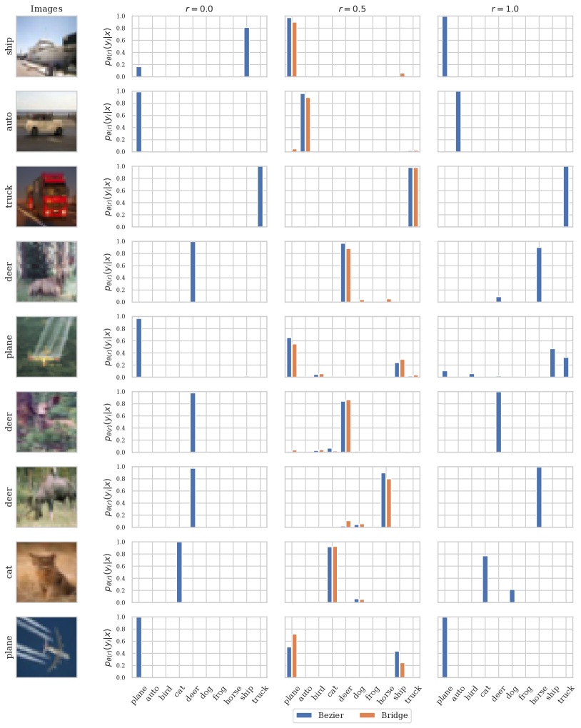
Figure 9: Bar plots in the third column depict whether the bridge network (orange) outputs the same class probability values as the base model with the Bezier parameters ${\boldsymbol{\theta}}^{(\text{be})}_{1,2}(0.5)$ (blue), for a given test inputs displayed in the first column. We also depict the predicted logits from ${\boldsymbol{\theta}}_{1}$ and ${\boldsymbol{\theta}}_{2}$ in the second and fourth columns, respectively.

B.7 Full type I and type II bridge results

We report full experimental results for classification tasks; (1) Type I bridge network results in Table 10, Table 12, Table 14 and Table 16, (2) Type II bridge network results in Table 11, Table 13, Table 15 and Table 17.

B.8 Full type I and type II bridge results with Batch Normalization

We report complete experimental results for classification tasks with Batch Normalization instead of Filter Response Normalization; (1) Type I bridge network results in Table 18, Table 20 and Table 22, (2) Type II bridge network results in Table 19, Table 21 and Table 23. The results indicate that the choice of a normalization operation is an architectural detail, and our approach is also compatible with conventional Batch Normalization.

Table 10: Full result of performance improvement of the ensemble by adding type I bridges on CIFAR-10 dataset. We use the same settings as described in Table 2.

CIFAR-10
Model	FLOPs ($\downarrow$)	#Params ($\downarrow$)	ACC ($\uparrow$)	NLL ($\downarrow$)	ECE ($\downarrow$)	BS ($\downarrow$)	DEE ($\uparrow$)
ResNet (de-1)	$\times$ 1.000	$\times$ 1.000	91.78 $\pm{\,0.10}$	0.287 $\pm{\,0.001}$	0.019 $\pm{\,0.001}$	0.126 $\pm{\,0.001}$	1.000
+ 1 Bridge${}_{\text{sm}}$	$\times$ 1.062	$\times$ 1.048	92.10 $\pm{\,0.04}$	0.252 $\pm{\,0.001}$	0.011 $\pm{\,0.001}$	0.118 $\pm{\,0.000}$	1.645 $\pm{\,0.041}$
+ 2 Bridge${}_{\text{sm}}$	$\times$ 1.125	$\times$ 1.097	92.15 $\pm{\,0.04}$	0.246 $\pm{\,0.001}$	0.009 $\pm{\,0.000}$	0.117 $\pm{\,0.000}$	1.759 $\pm{\,0.051}$
+ 3 Bridge${}_{\text{sm}}$	$\times$ 1.187	$\times$ 1.145	92.18 $\pm{\,0.04}$	0.244 $\pm{\,0.001}$	0.011 $\pm{\,0.000}$	0.116 $\pm{\,0.000}$	1.801 $\pm{\,0.055}$
+ 4 Bridge${}_{\text{sm}}$	$\times$ 1.249	$\times$ 1.194	92.22 $\pm{\,0.06}$	0.243 $\pm{\,0.000}$	0.010 $\pm{\,0.001}$	0.116 $\pm{\,0.000}$	1.819 $\pm{\,0.046}$
+ 1 Bridge${}_{\text{md}}$	$\times$ 1.205	$\times$ 1.159	92.09 $\pm{\,0.08}$	0.251 $\pm{\,0.001}$	0.011 $\pm{\,0.000}$	0.118 $\pm{\,0.000}$	1.674 $\pm{\,0.029}$
+ 2 Bridge${}_{\text{md}}$	$\times$ 1.411	$\times$ 1.319	92.20 $\pm{\,0.05}$	0.244 $\pm{\,0.001}$	0.010 $\pm{\,0.001}$	0.116 $\pm{\,0.000}$	1.797 $\pm{\,0.045}$
+ 3 Bridge${}_{\text{md}}$	$\times$ 1.616	$\times$ 1.478	92.23 $\pm{\,0.05}$	0.241 $\pm{\,0.000}$	0.009 $\pm{\,0.000}$	0.115 $\pm{\,0.000}$	1.850 $\pm{\,0.047}$
+ 4 Bridge${}_{\text{md}}$	$\times$ 1.822	$\times$ 1.638	92.29 $\pm{\,0.03}$	0.240 $\pm{\,0.000}$	0.010 $\pm{\,0.001}$	0.115 $\pm{\,0.000}$	1.874 $\pm{\,0.045}$
de-2	$\times$ 2.000	$\times$ 2.000	93.07 $\pm{\,0.11}$	0.233 $\pm{\,0.003}$	0.012 $\pm{\,0.001}$	0.107 $\pm{\,0.001}$	2.000

Table 11: Full result of performance improvement of the ensemble by adding type II bridges on CIFAR-10 dataset. We use the same settings as described in Table 3.

CIFAR-10
Model	FLOPs ($\downarrow$)	#Params ($\downarrow$)	ACC ($\uparrow$)	NLL ($\downarrow$)	ECE ($\downarrow$)	BS ($\downarrow$)	DEE ($\uparrow$)
de-2	$\times$ 2.000	$\times$ 2.000	93.07 $\pm{\,0.11}$	0.233 $\pm{\,0.003}$	0.012 $\pm{\,0.001}$	0.107 $\pm{\,0.001}$	2.000
+ 1 Bridge${}_{\text{sm}}$	$\times$ 2.081	$\times$ 2.063	93.09 $\pm{\,0.09}$	0.219 $\pm{\,0.003}$	0.007 $\pm{\,0.001}$	0.103 $\pm{\,0.001}$	2.811 $\pm{\,0.143}$
+ 1 Bridge${}_{\text{md}}$	$\times$ 2.247	$\times$ 2.192	93.09 $\pm{\,0.15}$	0.219 $\pm{\,0.003}$	0.007 $\pm{\,0.001}$	0.103 $\pm{\,0.001}$	2.837 $\pm{\,0.160}$
+ 1 Bezier	$\times$ 3.000	$\times$ 3.000	93.03 $\pm{\,0.11}$	0.227 $\pm{\,0.004}$	0.008 $\pm{\,0.001}$	0.105 $\pm{\,0.001}$	2.377 $\pm{\,0.090}$
de-3	$\times$ 3.000	$\times$ 3.000	93.37 $\pm{\,0.03}$	0.216 $\pm{\,0.004}$	0.009 $\pm{\,0.001}$	0.100 $\pm{\,0.001}$	3.000
+ 1 Bridge${}_{\text{sm}}$	$\times$ 3.081	$\times$ 3.063	93.45 $\pm{\,0.08}$	0.206 $\pm{\,0.002}$	0.006 $\pm{\,0.002}$	0.097 $\pm{\,0.001}$	3.896 $\pm{\,0.115}$
+ 2 Bridge${}_{\text{sm}}$	$\times$ 3.162	$\times$ 3.125	93.49 $\pm{\,0.10}$	0.203 $\pm{\,0.002}$	0.006 $\pm{\,0.001}$	0.097 $\pm{\,0.001}$	4.343 $\pm{\,0.213}$
+ 3 Bridge${}_{\text{sm}}$	$\times$ 3.244	$\times$ 3.188	93.52 $\pm{\,0.07}$	0.201 $\pm{\,0.002}$	0.006 $\pm{\,0.001}$	0.096 $\pm{\,0.001}$	4.629 $\pm{\,0.159}$
+ 1 Bridge${}_{\text{md}}$	$\times$ 3.247	$\times$ 3.192	93.48 $\pm{\,0.05}$	0.206 $\pm{\,0.003}$	0.007 $\pm{\,0.001}$	0.097 $\pm{\,0.001}$	3.899 $\pm{\,0.128}$
+ 2 Bridge${}_{\text{md}}$	$\times$ 3.494	$\times$ 3.384	93.53 $\pm{\,0.09}$	0.203 $\pm{\,0.002}$	0.006 $\pm{\,0.000}$	0.096 $\pm{\,0.001}$	4.346 $\pm{\,0.248}$
+ 3 Bridge${}_{\text{md}}$	$\times$ 3.741	$\times$ 3.575	93.52 $\pm{\,0.08}$	0.201 $\pm{\,0.002}$	0.007 $\pm{\,0.001}$	0.096 $\pm{\,0.001}$	4.658 $\pm{\,0.245}$
+ 3 Bezier	$\times$ 6.000	$\times$ 6.000	93.37 $\pm{\,0.14}$	0.208 $\pm{\,0.003}$	0.006 $\pm{\,0.000}$	0.098 $\pm{\,0.001}$	3.752 $\pm{\,0.194}$
de-4	$\times$ 4.000	$\times$ 4.000	93.59 $\pm{\,0.10}$	0.205 $\pm{\,0.002}$	0.010 $\pm{\,0.001}$	0.096 $\pm{\,0.001}$	4.000
+ 1 Bridge${}_{\text{sm}}$	$\times$ 4.081	$\times$ 4.063	93.54 $\pm{\,0.06}$	0.199 $\pm{\,0.002}$	0.008 $\pm{\,0.002}$	0.094 $\pm{\,0.001}$	5.040 $\pm{\,0.050}$
+ 2 Bridge${}_{\text{sm}}$	$\times$ 4.162	$\times$ 4.125	93.60 $\pm{\,0.08}$	0.197 $\pm{\,0.002}$	0.006 $\pm{\,0.001}$	0.094 $\pm{\,0.001}$	5.458 $\pm{\,0.099}$
+ 3 Bridge${}_{\text{sm}}$	$\times$ 4.244	$\times$ 4.188	93.60 $\pm{\,0.06}$	0.195 $\pm{\,0.002}$	0.006 $\pm{\,0.001}$	0.094 $\pm{\,0.001}$	5.678 $\pm{\,0.115}$
+ 4 Bridge${}_{\text{sm}}$	$\times$ 4.325	$\times$ 4.251	93.57 $\pm{\,0.03}$	0.195 $\pm{\,0.002}$	0.006 $\pm{\,0.000}$	0.093 $\pm{\,0.001}$	5.869 $\pm{\,0.177}$
+ 5 Bridge${}_{\text{sm}}$	$\times$ 4.406	$\times$ 4.314	93.55 $\pm{\,0.05}$	0.194 $\pm{\,0.002}$	0.005 $\pm{\,0.000}$	0.093 $\pm{\,0.001}$	5.950 $\pm{\,0.212}$
+ 6 Bridge${}_{\text{sm}}$	$\times$ 4.487	$\times$ 4.376	93.58 $\pm{\,0.04}$	0.194 $\pm{\,0.002}$	0.006 $\pm{\,0.000}$	0.094 $\pm{\,0.001}$	5.997 $\pm{\,0.172}$
+ 1 Bridge${}_{\text{md}}$	$\times$ 4.247	$\times$ 4.192	93.56 $\pm{\,0.08}$	0.199 $\pm{\,0.002}$	0.009 $\pm{\,0.001}$	0.094 $\pm{\,0.001}$	5.006 $\pm{\,0.086}$
+ 2 Bridge${}_{\text{md}}$	$\times$ 4.494	$\times$ 4.384	93.63 $\pm{\,0.10}$	0.197 $\pm{\,0.002}$	0.007 $\pm{\,0.001}$	0.093 $\pm{\,0.001}$	5.415 $\pm{\,0.120}$
+ 3 Bridge${}_{\text{md}}$	$\times$ 4.741	$\times$ 4.575	93.63 $\pm{\,0.07}$	0.196 $\pm{\,0.002}$	0.007 $\pm{\,0.001}$	0.093 $\pm{\,0.001}$	5.646 $\pm{\,0.123}$
+ 4 Bridge${}_{\text{md}}$	$\times$ 4.988	$\times$ 4.767	93.67 $\pm{\,0.07}$	0.195 $\pm{\,0.002}$	0.007 $\pm{\,0.001}$	0.093 $\pm{\,0.001}$	5.857 $\pm{\,0.165}$
+ 5 Bridge${}_{\text{md}}$	$\times$ 5.236	$\times$ 4.959	93.62 $\pm{\,0.04}$	0.194 $\pm{\,0.002}$	0.006 $\pm{\,0.000}$	0.093 $\pm{\,0.001}$	6.008 $\pm{\,0.206}$
+ 6 Bridge${}_{\text{md}}$	$\times$ 5.483	$\times$ 5.151	93.57 $\pm{\,0.03}$	0.194 $\pm{\,0.002}$	0.006 $\pm{\,0.000}$	0.093 $\pm{\,0.001}$	6.086 $\pm{\,0.233}$
+ 6 Bezier	$\times$ 10.000	$\times$ 10.000	93.59 $\pm{\,0.11}$	0.198 $\pm{\,0.002}$	0.007 $\pm{\,0.001}$	0.094 $\pm{\,0.001}$	5.109 $\pm{\,0.212}$
de-5	$\times$ 5.000	$\times$ 5.000	93.68 $\pm{\,0.10}$	0.199 $\pm{\,0.002}$	0.011 $\pm{\,0.001}$	0.093 $\pm{\,0.001}$	5.000

Table 12: Full result of performance improvement of the ensemble by adding type I bridges on CIFAR-100 dataset. We use the same settings as described in Table 2.

CIFAR-100
Model	FLOPs ($\downarrow$)	#Params ($\downarrow$)	ACC ($\uparrow$)	NLL ($\downarrow$)	ECE ($\downarrow$)	BS ($\downarrow$)	DEE ($\uparrow$)
ResNet (de-1)	$\times$ 1.000	$\times$ 1.000	74.06 $\pm{\,0.31}$	1.060 $\pm{\,0.005}$	0.047 $\pm{\,0.003}$	0.367 $\pm{\,0.002}$	1.000
+ 1 Bridge${}_{\text{sm}}$	$\times$ 1.063	$\times$ 1.048	75.03 $\pm{\,0.07}$	0.938 $\pm{\,0.001}$	0.029 $\pm{\,0.001}$	0.347 $\pm{\,0.000}$	1.928 $\pm{\,0.038}$
+ 2 Bridge${}_{\text{sm}}$	$\times$ 1.127	$\times$ 1.097	75.47 $\pm{\,0.11}$	0.911 $\pm{\,0.001}$	0.025 $\pm{\,0.000}$	0.342 $\pm{\,0.001}$	2.321 $\pm{\,0.076}$
+ 3 Bridge${}_{\text{sm}}$	$\times$ 1.190	$\times$ 1.145	75.58 $\pm{\,0.16}$	0.900 $\pm{\,0.001}$	0.025 $\pm{\,0.001}$	0.340 $\pm{\,0.000}$	2.545 $\pm{\,0.077}$
+ 4 Bridge${}_{\text{sm}}$	$\times$ 1.253	$\times$ 1.194	75.58 $\pm{\,0.07}$	0.893 $\pm{\,0.001}$	0.024 $\pm{\,0.001}$	0.339 $\pm{\,0.000}$	2.673 $\pm{\,0.070}$
+ 1 Bridge${}_{\text{md}}$	$\times$ 1.210	$\times$ 1.160	75.25 $\pm{\,0.09}$	0.929 $\pm{\,0.003}$	0.033 $\pm{\,0.001}$	0.344 $\pm{\,0.001}$	2.008 $\pm{\,0.042}$
+ 2 Bridge${}_{\text{md}}$	$\times$ 1.419	$\times$ 1.320	75.64 $\pm{\,0.05}$	0.901 $\pm{\,0.002}$	0.030 $\pm{\,0.001}$	0.339 $\pm{\,0.000}$	2.517 $\pm{\,0.068}$
+ 3 Bridge${}_{\text{md}}$	$\times$ 1.629	$\times$ 1.480	75.71 $\pm{\,0.03}$	0.888 $\pm{\,0.001}$	0.031 $\pm{\,0.001}$	0.337 $\pm{\,0.000}$	2.765 $\pm{\,0.081}$
+ 4 Bridge${}_{\text{md}}$	$\times$ 1.838	$\times$ 1.640	75.85 $\pm{\,0.10}$	0.882 $\pm{\,0.001}$	0.030 $\pm{\,0.001}$	0.336 $\pm{\,0.000}$	2.895 $\pm{\,0.061}$
de-2	$\times$ 2.000	$\times$ 2.000	76.21 $\pm{\,0.11}$	0.928 $\pm{\,0.004}$	0.027 $\pm{\,0.003}$	0.334 $\pm{\,0.001}$	2.000

Table 13: Full result of performance improvement of the ensemble by adding type II bridges on CIFAR-100 dataset. We use the same settings as described in Table 3.

CIFAR-100
Model	FLOPs ($\downarrow$)	#Params ($\downarrow$)	ACC ($\uparrow$)	NLL ($\downarrow$)	ECE ($\downarrow$)	BS ($\downarrow$)	DEE ($\uparrow$)
de-2	$\times$ 2.000	$\times$ 2.000	76.21 $\pm{\,0.11}$	0.928 $\pm{\,0.004}$	0.027 $\pm{\,0.003}$	0.334 $\pm{\,0.001}$	2.000
+ 1 Bridge${}_{\text{sm}}$	$\times$ 2.083	$\times$ 2.063	76.72 $\pm{\,0.19}$	0.868 $\pm{\,0.001}$	0.025 $\pm{\,0.001}$	0.325 $\pm{\,0.001}$	3.256 $\pm{\,0.096}$
+ 1 Bridge${}_{\text{md}}$	$\times$ 2.252	$\times$ 2.192	76.75 $\pm{\,0.12}$	0.863 $\pm{\,0.003}$	0.024 $\pm{\,0.002}$	0.324 $\pm{\,0.001}$	3.435 $\pm{\,0.065}$
+ 1 Bezier	$\times$ 3.000	$\times$ 3.000	76.87 $\pm{\,0.10}$	0.879 $\pm{\,0.005}$	0.021 $\pm{\,0.002}$	0.324 $\pm{\,0.001}$	2.954 $\pm{\,0.111}$
de-3	$\times$ 3.000	$\times$ 3.000	77.23 $\pm{\,0.18}$	0.876 $\pm{\,0.003}$	0.024 $\pm{\,0.001}$	0.321 $\pm{\,0.001}$	3.000
+ 1 Bridge${}_{\text{sm}}$	$\times$ 3.083	$\times$ 3.063	77.43 $\pm{\,0.09}$	0.838 $\pm{\,0.001}$	0.021 $\pm{\,0.002}$	0.316 $\pm{\,0.001}$	4.429 $\pm{\,0.112}$
+ 2 Bridge${}_{\text{sm}}$	$\times$ 3.165	$\times$ 3.126	77.62 $\pm{\,0.08}$	0.822 $\pm{\,0.002}$	0.019 $\pm{\,0.001}$	0.314 $\pm{\,0.000}$	5.387 $\pm{\,0.168}$
+ 3 Bridge${}_{\text{sm}}$	$\times$ 3.248	$\times$ 3.190	77.67 $\pm{\,0.09}$	0.813 $\pm{\,0.003}$	0.020 $\pm{\,0.002}$	0.313 $\pm{\,0.000}$	5.980 $\pm{\,0.289}$
+ 1 Bridge${}_{\text{md}}$	$\times$ 3.252	$\times$ 3.192	77.53 $\pm{\,0.13}$	0.835 $\pm{\,0.002}$	0.021 $\pm{\,0.002}$	0.315 $\pm{\,0.001}$	4.581 $\pm{\,0.097}$
+ 2 Bridge${}_{\text{md}}$	$\times$ 3.504	$\times$ 3.385	77.71 $\pm{\,0.05}$	0.818 $\pm{\,0.002}$	0.022 $\pm{\,0.001}$	0.312 $\pm{\,0.000}$	5.655 $\pm{\,0.093}$
+ 3 Bridge${}_{\text{md}}$	$\times$ 3.756	$\times$ 3.577	77.77 $\pm{\,0.05}$	0.809 $\pm{\,0.003}$	0.023 $\pm{\,0.001}$	0.311 $\pm{\,0.000}$	6.304 $\pm{\,0.236}$
+ 3 Bezier	$\times$ 6.000	$\times$ 6.000	77.92 $\pm{\,0.04}$	0.816 $\pm{\,0.004}$	0.018 $\pm{\,0.002}$	0.310 $\pm{\,0.001}$	5.782 $\pm{\,0.254}$
de-4	$\times$ 4.000	$\times$ 4.000	77.79 $\pm{\,0.21}$	0.846 $\pm{\,0.001}$	0.023 $\pm{\,0.002}$	0.313 $\pm{\,0.001}$	4.000
+ 1 Bridge${}_{\text{sm}}$	$\times$ 4.083	$\times$ 4.063	77.85 $\pm{\,0.19}$	0.819 $\pm{\,0.002}$	0.020 $\pm{\,0.001}$	0.310 $\pm{\,0.001}$	5.570 $\pm{\,0.120}$
+ 2 Bridge${}_{\text{sm}}$	$\times$ 4.165	$\times$ 4.126	77.92 $\pm{\,0.14}$	0.807 $\pm{\,0.002}$	0.019 $\pm{\,0.002}$	0.309 $\pm{\,0.000}$	6.481 $\pm{\,0.202}$
+ 3 Bridge${}_{\text{sm}}$	$\times$ 4.248	$\times$ 4.190	78.07 $\pm{\,0.09}$	0.799 $\pm{\,0.002}$	0.021 $\pm{\,0.001}$	0.308 $\pm{\,0.000}$	7.079 $\pm{\,0.121}$
+ 4 Bridge${}_{\text{sm}}$	$\times$ 4.330	$\times$ 4.253	78.09 $\pm{\,0.07}$	0.794 $\pm{\,0.002}$	0.020 $\pm{\,0.002}$	0.307 $\pm{\,0.000}$	7.505 $\pm{\,0.168}$
+ 5 Bridge${}_{\text{sm}}$	$\times$ 4.413	$\times$ 4.316	78.13 $\pm{\,0.18}$	0.790 $\pm{\,0.001}$	0.020 $\pm{\,0.001}$	0.307 $\pm{\,0.000}$	7.858 $\pm{\,0.119}$
+ 6 Bridge${}_{\text{sm}}$	$\times$ 4.496	$\times$ 4.379	78.15 $\pm{\,0.20}$	0.788 $\pm{\,0.002}$	0.020 $\pm{\,0.002}$	0.307 $\pm{\,0.000}$	8.036 $\pm{\,0.104}$
+ 1 Bridge${}_{\text{md}}$	$\times$ 4.252	$\times$ 4.192	77.91 $\pm{\,0.14}$	0.817 $\pm{\,0.002}$	0.020 $\pm{\,0.001}$	0.309 $\pm{\,0.001}$	5.671 $\pm{\,0.057}$
+ 2 Bridge${}_{\text{md}}$	$\times$ 4.504	$\times$ 4.385	78.05 $\pm{\,0.15}$	0.804 $\pm{\,0.002}$	0.021 $\pm{\,0.001}$	0.308 $\pm{\,0.001}$	6.696 $\pm{\,0.105}$
+ 3 Bridge${}_{\text{md}}$	$\times$ 4.756	$\times$ 4.577	78.06 $\pm{\,0.06}$	0.796 $\pm{\,0.002}$	0.020 $\pm{\,0.001}$	0.306 $\pm{\,0.000}$	7.363 $\pm{\,0.087}$
+ 4 Bridge${}_{\text{md}}$	$\times$ 5.008	$\times$ 4.770	78.17 $\pm{\,0.12}$	0.791 $\pm{\,0.001}$	0.021 $\pm{\,0.001}$	0.306 $\pm{\,0.000}$	7.831 $\pm{\,0.052}$
+ 5 Bridge${}_{\text{md}}$	$\times$ 5.260	$\times$ 4.962	78.19 $\pm{\,0.08}$	0.786 $\pm{\,0.001}$	0.021 $\pm{\,0.002}$	0.305 $\pm{\,0.000}$	8.182 $\pm{\,0.027}$
+ 6 Bridge${}_{\text{md}}$	$\times$ 5.512	$\times$ 5.154	78.24 $\pm{\,0.10}$	0.784 $\pm{\,0.002}$	0.021 $\pm{\,0.001}$	0.305 $\pm{\,0.000}$	8.382 $\pm{\,0.073}$
+ 6 Bezier	$\times$ 10.000	$\times$ 10.000	78.36 $\pm{\,0.05}$	0.787 $\pm{\,0.003}$	0.016 $\pm{\,0.001}$	0.303 $\pm{\,0.001}$	8.178 $\pm{\,0.144}$
de-5	$\times$ 5.000	$\times$ 5.000	78.21 $\pm{\,0.08}$	0.827 $\pm{\,0.003}$	0.024 $\pm{\,0.002}$	0.308 $\pm{\,0.000}$	5.000

Table 14: Full result of performance improvement of the ensemble by adding type I bridges on Tiny ImageNet dataset. We use the same settings as described in Table 2.

Tiny ImageNet
Model	FLOPs ($\downarrow$)	#Params ($\downarrow$)	ACC ($\uparrow$)	NLL ($\downarrow$)	ECE ($\downarrow$)	BS ($\downarrow$)	DEE ($\uparrow$)
ResNet (de-1)	$\times$ 1.000	$\times$ 1.000	62.66 $\pm{\,0.23}$	1.683 $\pm{\,0.009}$	0.050 $\pm{\,0.004}$	0.499 $\pm{\,0.002}$	1.000
+ 1 Bridge${}_{\text{sm}}$	$\times$ 1.050	$\times$ 1.057	64.58 $\pm{\,0.17}$	1.478 $\pm{\,0.006}$	0.025 $\pm{\,0.002}$	0.469 $\pm{\,0.001}$	2.280 $\pm{\,0.086}$
+ 2 Bridge${}_{\text{sm}}$	$\times$ 1.099	$\times$ 1.114	65.37 $\pm{\,0.13}$	1.421 $\pm{\,0.004}$	0.018 $\pm{\,0.002}$	0.459 $\pm{\,0.000}$	3.087 $\pm{\,0.118}$
+ 3 Bridge${}_{\text{sm}}$	$\times$ 1.149	$\times$ 1.171	65.82 $\pm{\,0.10}$	1.395 $\pm{\,0.003}$	0.015 $\pm{\,0.001}$	0.454 $\pm{\,0.001}$	3.680 $\pm{\,0.133}$
+ 4 Bridge${}_{\text{sm}}$	$\times$ 1.198	$\times$ 1.228	65.93 $\pm{\,0.10}$	1.380 $\pm{\,0.001}$	0.014 $\pm{\,0.002}$	0.452 $\pm{\,0.000}$	4.061 $\pm{\,0.157}$
+ 1 Bridge${}_{\text{md}}$	$\times$ 1.180	$\times$ 1.206	65.13 $\pm{\,0.12}$	1.446 $\pm{\,0.002}$	0.034 $\pm{\,0.002}$	0.461 $\pm{\,0.001}$	2.709 $\pm{\,0.049}$
+ 2 Bridge${}_{\text{md}}$	$\times$ 1.359	$\times$ 1.412	66.29 $\pm{\,0.06}$	1.388 $\pm{\,0.004}$	0.025 $\pm{\,0.001}$	0.449 $\pm{\,0.000}$	3.845 $\pm{\,0.171}$
+ 3 Bridge${}_{\text{md}}$	$\times$ 1.539	$\times$ 1.618	66.76 $\pm{\,0.09}$	1.362 $\pm{\,0.003}$	0.023 $\pm{\,0.001}$	0.443 $\pm{\,0.000}$	4.708 $\pm{\,0.209}$
+ 4 Bridge${}_{\text{md}}$	$\times$ 1.719	$\times$ 1.824	66.96 $\pm{\,0.06}$	1.347 $\pm{\,0.002}$	0.023 $\pm{\,0.001}$	0.440 $\pm{\,0.000}$	5.372 $\pm{\,0.169}$
de-2	$\times$ 2.000	$\times$ 2.000	65.54 $\pm{\,0.25}$	1.499 $\pm{\,0.007}$	0.029 $\pm{\,0.003}$	0.461 $\pm{\,0.001}$	2.000

Table 15: Full result of performance improvement of the ensemble by adding type II bridges on Tiny ImageNet dataset. We use the same settings as described in Table 3.

Tiny ImageNet
Model	FLOPs ($\downarrow$)	#Params ($\downarrow$)	ACC ($\uparrow$)	NLL ($\downarrow$)	ECE ($\downarrow$)	BS ($\downarrow$)	DEE ($\uparrow$)
de-2	$\times$ 2.000	$\times$ 2.000	65.54 $\pm{\,0.25}$	1.499 $\pm{\,0.007}$	0.029 $\pm{\,0.003}$	0.461 $\pm{\,0.001}$	2.000
+ 1 Bridge${}_{\text{sm}}$	$\times$ 2.058	$\times$ 2.067	66.66 $\pm{\,0.37}$	1.394 $\pm{\,0.007}$	0.021 $\pm{\,0.002}$	0.445 $\pm{\,0.001}$	3.708 $\pm{\,0.187}$
+ 1 Bridge${}_{\text{md}}$	$\times$ 2.198	$\times$ 2.226	66.72 $\pm{\,0.15}$	1.386 $\pm{\,0.005}$	0.025 $\pm{\,0.001}$	0.443 $\pm{\,0.001}$	3.901 $\pm{\,0.109}$
+ 1 Bezier	$\times$ 3.000	$\times$ 3.000	66.17 $\pm{\,0.12}$	1.436 $\pm{\,0.004}$	0.024 $\pm{\,0.001}$	0.449 $\pm{\,0.001}$	2.851 $\pm{\,0.059}$
de-3	$\times$ 3.000	$\times$ 3.000	66.65 $\pm{\,0.18}$	1.425 $\pm{\,0.005}$	0.024 $\pm{\,0.002}$	0.444 $\pm{\,0.001}$	3.000
+ 1 Bridge${}_{\text{sm}}$	$\times$ 3.058	$\times$ 3.067	67.38 $\pm{\,0.18}$	1.358 $\pm{\,0.005}$	0.016 $\pm{\,0.001}$	0.435 $\pm{\,0.001}$	4.868 $\pm{\,0.189}$
+ 2 Bridge${}_{\text{sm}}$	$\times$ 3.117	$\times$ 3.135	67.80 $\pm{\,0.04}$	1.328 $\pm{\,0.007}$	0.017 $\pm{\,0.001}$	0.430 $\pm{\,0.002}$	6.632 $\pm{\,0.640}$
+ 3 Bridge${}_{\text{sm}}$	$\times$ 3.175	$\times$ 3.202	68.06 $\pm{\,0.26}$	1.312 $\pm{\,0.006}$	0.016 $\pm{\,0.001}$	0.428 $\pm{\,0.001}$	8.092 $\pm{\,0.610}$
+ 1 Bridge${}_{\text{md}}$	$\times$ 3.198	$\times$ 3.226	67.47 $\pm{\,0.11}$	1.354 $\pm{\,0.006}$	0.020 $\pm{\,0.001}$	0.433 $\pm{\,0.001}$	5.028 $\pm{\,0.192}$
+ 2 Bridge${}_{\text{md}}$	$\times$ 3.395	$\times$ 3.453	67.97 $\pm{\,0.10}$	1.322 $\pm{\,0.005}$	0.022 $\pm{\,0.002}$	0.428 $\pm{\,0.001}$	7.196 $\pm{\,0.521}$
+ 3 Bridge${}_{\text{md}}$	$\times$ 3.593	$\times$ 3.679	68.22 $\pm{\,0.09}$	1.303 $\pm{\,0.006}$	0.022 $\pm{\,0.002}$	0.425 $\pm{\,0.001}$	8.931 $\pm{\,0.627}$
+ 3 Bezier	$\times$ 6.000	$\times$ 6.000	67.80 $\pm{\,0.12}$	1.344 $\pm{\,0.004}$	0.019 $\pm{\,0.003}$	0.430 $\pm{\,0.000}$	5.513 $\pm{\,0.162}$
de-4	$\times$ 4.000	$\times$ 4.000	67.50 $\pm{\,0.11}$	1.381 $\pm{\,0.004}$	0.018 $\pm{\,0.001}$	0.435 $\pm{\,0.001}$	4.000
+ 1 Bridge${}_{\text{sm}}$	$\times$ 4.058	$\times$ 4.067	67.86 $\pm{\,0.05}$	1.334 $\pm{\,0.003}$	0.017 $\pm{\,0.002}$	0.429 $\pm{\,0.001}$	6.051 $\pm{\,0.181}$
+ 2 Bridge${}_{\text{sm}}$	$\times$ 4.117	$\times$ 4.135	68.12 $\pm{\,0.09}$	1.311 $\pm{\,0.005}$	0.015 $\pm{\,0.001}$	0.425 $\pm{\,0.001}$	8.174 $\pm{\,0.465}$
+ 3 Bridge${}_{\text{sm}}$	$\times$ 4.175	$\times$ 4.202	68.42 $\pm{\,0.09}$	1.297 $\pm{\,0.004}$	0.015 $\pm{\,0.002}$	0.424 $\pm{\,0.001}$	9.508 $\pm{\,0.633}$
+ 4 Bridge${}_{\text{sm}}$	$\times$ 4.234	$\times$ 4.269	68.47 $\pm{\,0.14}$	1.288 $\pm{\,0.004}$	0.015 $\pm{\,0.001}$	0.422 $\pm{\,0.001}$	10.340 $\pm{\,0.773}$
+ 5 Bridge${}_{\text{sm}}$	$\times$ 4.292	$\times$ 4.337	68.49 $\pm{\,0.25}$	1.282 $\pm{\,0.004}$	0.015 $\pm{\,0.001}$	0.422 $\pm{\,0.001}$	10.861 $\pm{\,0.829}$
+ 6 Bridge${}_{\text{sm}}$	$\times$ 4.351	$\times$ 4.404	68.51 $\pm{\,0.10}$	1.278 $\pm{\,0.003}$	0.014 $\pm{\,0.001}$	0.421 $\pm{\,0.001}$	11.268 $\pm{\,0.871}$
+ 1 Bridge${}_{\text{md}}$	$\times$ 4.198	$\times$ 4.226	68.00 $\pm{\,0.11}$	1.333 $\pm{\,0.003}$	0.019 $\pm{\,0.001}$	0.428 $\pm{\,0.001}$	6.183 $\pm{\,0.120}$
+ 2 Bridge${}_{\text{md}}$	$\times$ 4.395	$\times$ 4.453	68.33 $\pm{\,0.08}$	1.308 $\pm{\,0.003}$	0.019 $\pm{\,0.001}$	0.424 $\pm{\,0.001}$	8.489 $\pm{\,0.481}$
+ 3 Bridge${}_{\text{md}}$	$\times$ 4.593	$\times$ 4.679	68.50 $\pm{\,0.06}$	1.293 $\pm{\,0.003}$	0.020 $\pm{\,0.001}$	0.422 $\pm{\,0.001}$	9.853 $\pm{\,0.679}$
+ 4 Bridge${}_{\text{md}}$	$\times$ 4.791	$\times$ 4.906	68.61 $\pm{\,0.05}$	1.281 $\pm{\,0.004}$	0.021 $\pm{\,0.003}$	0.420 $\pm{\,0.001}$	10.897 $\pm{\,0.800}$
+ 5 Bridge${}_{\text{md}}$	$\times$ 4.988	$\times$ 5.132	68.70 $\pm{\,0.10}$	1.274 $\pm{\,0.003}$	0.023 $\pm{\,0.001}$	0.419 $\pm{\,0.001}$	11.560 $\pm{\,0.964}$
+ 6 Bridge${}_{\text{md}}$	$\times$ 5.186	$\times$ 5.359	68.80 $\pm{\,0.09}$	1.269 $\pm{\,0.003}$	0.021 $\pm{\,0.001}$	0.418 $\pm{\,0.001}$	12.110 $\pm{\,1.083}$
+ 6 Bezier	$\times$ 10.000	$\times$ 10.000	68.51 $\pm{\,0.18}$	1.299 $\pm{\,0.002}$	0.020 $\pm{\,0.001}$	0.421 $\pm{\,0.000}$	9.312 $\pm{\,0.610}$
de-5	$\times$ 5.000	$\times$ 5.000	67.90 $\pm{\,0.14}$	1.354 $\pm{\,0.003}$	0.019 $\pm{\,0.001}$	0.429 $\pm{\,0.001}$	5.000

Table 16: Full result of performance improvement of the ensemble by adding type I bridges on ImageNet dataset. We use the same settings as described in Table 2.

ImageNet
Model	FLOPs ($\downarrow$)	#Params ($\downarrow$)	ACC ($\uparrow$)	NLL ($\downarrow$)	ECE ($\downarrow$)	BS ($\downarrow$)	DEE ($\uparrow$)
ResNet (de-1)	$\times$ 1.000	$\times$ 1.000	75.85 $\pm{\,0.06}$	0.936 $\pm{\,0.003}$	0.019 $\pm{\,0.001}$	0.333 $\pm{\,0.001}$	1.000
+ 1 Bridge${}_{\text{sm}}$	$\times$ 1.061	$\times$ 1.071	76.46 $\pm{\,0.06}$	0.914 $\pm{\,0.000}$	0.012 $\pm{\,0.001}$	0.326 $\pm{\,0.000}$	1.418 $\pm{\,0.034}$
+ 2 Bridge${}_{\text{sm}}$	$\times$ 1.123	$\times$ 1.141	76.60 $\pm{\,0.06}$	0.907 $\pm{\,0.000}$	0.012 $\pm{\,0.001}$	0.324 $\pm{\,0.000}$	1.537 $\pm{\,0.026}$
+ 3 Bridge${}_{\text{sm}}$	$\times$ 1.184	$\times$ 1.212	76.69 $\pm{\,0.04}$	0.905 $\pm{\,0.000}$	0.011 $\pm{\,0.001}$	0.323 $\pm{\,0.000}$	1.584 $\pm{\,0.021}$
+ 4 Bridge${}_{\text{sm}}$	$\times$ 1.245	$\times$ 1.283	76.71 $\pm{\,0.03}$	0.904 $\pm{\,0.000}$	0.011 $\pm{\,0.001}$	0.322 $\pm{\,0.000}$	1.610 $\pm{\,0.021}$
+ 1 Bridge${}_{\text{md}}$	$\times$ 1.194	$\times$ 1.222	77.03 $\pm{\,0.07}$	0.889 $\pm{\,0.001}$	0.013 $\pm{\,0.000}$	0.319 $\pm{\,0.000}$	1.881 $\pm{\,0.022}$
+ 2 Bridge${}_{\text{md}}$	$\times$ 1.389	$\times$ 1.444	77.37 $\pm{\,0.07}$	0.876 $\pm{\,0.001}$	0.013 $\pm{\,0.001}$	0.315 $\pm{\,0.000}$	2.341 $\pm{\,0.076}$
+ 3 Bridge${}_{\text{md}}$	$\times$ 1.583	$\times$ 1.665	77.48 $\pm{\,0.03}$	0.870 $\pm{\,0.000}$	0.013 $\pm{\,0.000}$	0.313 $\pm{\,0.000}$	2.618 $\pm{\,0.062}$
+ 4 Bridge${}_{\text{md}}$	$\times$ 1.778	$\times$ 1.887	77.59 $\pm{\,0.04}$	0.867 $\pm{\,0.000}$	0.013 $\pm{\,0.000}$	0.312 $\pm{\,0.000}$	2.781 $\pm{\,0.069}$
de-2	$\times$ 2.000	$\times$ 2.000	77.12 $\pm{\,0.04}$	0.883 $\pm{\,0.001}$	0.012 $\pm{\,0.001}$	0.318 $\pm{\,0.000}$	2.000

Table 17: Full result of performance improvement of the ensemble by adding type II bridges on ImageNet dataset. We use the same settings as described in Table 3.

ImageNet
Model	FLOPs ($\downarrow$)	#Params ($\downarrow$)	ACC ($\uparrow$)	NLL ($\downarrow$)	ECE ($\downarrow$)	BS ($\downarrow$)	DEE ($\uparrow$)
de-2	$\times$ 2.000	$\times$ 2.000	77.12 $\pm{\,0.04}$	0.883 $\pm{\,0.001}$	0.012 $\pm{\,0.001}$	0.318 $\pm{\,0.000}$	2.000
+ 1 Bridge${}_{\text{sm}}$	$\times$ 2.086	$\times$ 2.088	77.44 $\pm{\,0.03}$	0.871 $\pm{\,0.001}$	0.012 $\pm{\,0.000}$	0.314 $\pm{\,0.000}$	2.567 $\pm{\,0.017}$
+ 1 Bridge${}_{\text{md}}$	$\times$ 2.243	$\times$ 2.256	77.70 $\pm{\,0.05}$	0.857 $\pm{\,0.001}$	0.012 $\pm{\,0.001}$	0.310 $\pm{\,0.000}$	3.416 $\pm{\,0.131}$
+ 1 Bezier	$\times$ 3.000	$\times$ 3.000	77.81 $\pm{\,0.10}$	0.854 $\pm{\,0.001}$	0.012 $\pm{\,0.001}$	0.309 $\pm{\,0.000}$	3.767 $\pm{\,0.137}$
de-3	$\times$ 3.000	$\times$ 3.000	77.64 $\pm{\,0.04}$	0.862 $\pm{\,0.001}$	0.013 $\pm{\,0.001}$	0.311 $\pm{\,0.000}$	3.000
+ 1 Bridge${}_{\text{sm}}$	$\times$ 3.086	$\times$ 3.088	77.77 $\pm{\,0.04}$	0.856 $\pm{\,0.001}$	0.012 $\pm{\,0.000}$	0.310 $\pm{\,0.000}$	3.536 $\pm{\,0.043}$
+ 2 Bridge${}_{\text{sm}}$	$\times$ 3.172	$\times$ 3.176	77.87 $\pm{\,0.02}$	0.854 $\pm{\,0.001}$	0.011 $\pm{\,0.000}$	0.309 $\pm{\,0.000}$	3.735 $\pm{\,0.053}$
+ 3 Bridge${}_{\text{sm}}$	$\times$ 3.257	$\times$ 3.263	77.94 $\pm{\,0.02}$	0.853 $\pm{\,0.001}$	0.012 $\pm{\,0.000}$	0.308 $\pm{\,0.000}$	3.779 $\pm{\,0.041}$
+ 1 Bridge${}_{\text{md}}$	$\times$ 3.243	$\times$ 3.256	77.95 $\pm{\,0.07}$	0.846 $\pm{\,0.000}$	0.012 $\pm{\,0.001}$	0.307 $\pm{\,0.000}$	4.670 $\pm{\,0.118}$
+ 2 Bridge${}_{\text{md}}$	$\times$ 3.487	$\times$ 3.512	78.16 $\pm{\,0.07}$	0.838 $\pm{\,0.001}$	0.012 $\pm{\,0.001}$	0.305 $\pm{\,0.000}$	6.438 $\pm{\,0.241}$
+ 3 Bridge${}_{\text{md}}$	$\times$ 3.730	$\times$ 3.768	78.28 $\pm{\,0.06}$	0.835 $\pm{\,0.001}$	0.012 $\pm{\,0.000}$	0.303 $\pm{\,0.000}$	7.610 $\pm{\,0.242}$
+ 3 Bezier	$\times$ 6.000	$\times$ 6.000	78.62 $\pm{\,0.05}$	0.823 $\pm{\,0.001}$	0.012 $\pm{\,0.001}$	0.300 $\pm{\,0.000}$	11.580 $\pm{\,0.410}$
de-4	$\times$ 4.000	$\times$ 4.000	77.87 $\pm{\,0.04}$	0.851 $\pm{\,0.001}$	0.012 $\pm{\,0.001}$	0.308 $\pm{\,0.000}$	4.000
+ 1 Bridge${}_{\text{sm}}$	$\times$ 4.086	$\times$ 4.088	77.93 $\pm{\,0.02}$	0.847 $\pm{\,0.000}$	0.012 $\pm{\,0.001}$	0.307 $\pm{\,0.000}$	4.580 $\pm{\,0.052}$
+ 2 Bridge${}_{\text{sm}}$	$\times$ 4.172	$\times$ 4.176	78.00 $\pm{\,0.04}$	0.846 $\pm{\,0.000}$	0.011 $\pm{\,0.000}$	0.307 $\pm{\,0.000}$	4.739 $\pm{\,0.052}$
+ 3 Bridge${}_{\text{sm}}$	$\times$ 4.257	$\times$ 4.263	78.07 $\pm{\,0.03}$	0.846 $\pm{\,0.000}$	0.011 $\pm{\,0.001}$	0.306 $\pm{\,0.000}$	4.775 $\pm{\,0.048}$
+ 4 Bridge${}_{\text{sm}}$	$\times$ 4.343	$\times$ 4.351	78.10 $\pm{\,0.03}$	0.846 $\pm{\,0.000}$	0.011 $\pm{\,0.001}$	0.306 $\pm{\,0.000}$	4.768 $\pm{\,0.041}$
+ 5 Bridge${}_{\text{sm}}$	$\times$ 4.429	$\times$ 4.439	78.14 $\pm{\,0.04}$	0.846 $\pm{\,0.000}$	0.012 $\pm{\,0.001}$	0.306 $\pm{\,0.000}$	4.724 $\pm{\,0.039}$
+ 6 Bridge${}_{\text{sm}}$	$\times$ 4.515	$\times$ 4.527	78.12 $\pm{\,0.05}$	0.846 $\pm{\,0.001}$	0.011 $\pm{\,0.001}$	0.306 $\pm{\,0.000}$	4.659 $\pm{\,0.037}$
+ 1 Bridge${}_{\text{md}}$	$\times$ 4.243	$\times$ 4.256	78.14 $\pm{\,0.03}$	0.839 $\pm{\,0.000}$	0.011 $\pm{\,0.001}$	0.305 $\pm{\,0.000}$	6.123 $\pm{\,0.121}$
+ 2 Bridge${}_{\text{md}}$	$\times$ 4.487	$\times$ 4.512	78.30 $\pm{\,0.05}$	0.833 $\pm{\,0.000}$	0.012 $\pm{\,0.001}$	0.303 $\pm{\,0.000}$	8.068 $\pm{\,0.144}$
+ 3 Bridge${}_{\text{md}}$	$\times$ 4.730	$\times$ 4.768	78.38 $\pm{\,0.05}$	0.830 $\pm{\,0.000}$	0.012 $\pm{\,0.001}$	0.302 $\pm{\,0.000}$	9.281 $\pm{\,0.126}$
+ 4 Bridge${}_{\text{md}}$	$\times$ 4.973	$\times$ 5.024	78.46 $\pm{\,0.04}$	0.828 $\pm{\,0.000}$	0.012 $\pm{\,0.000}$	0.301 $\pm{\,0.000}$	9.951 $\pm{\,0.163}$
+ 5 Bridge${}_{\text{md}}$	$\times$ 5.217	$\times$ 5.280	78.53 $\pm{\,0.07}$	0.826 $\pm{\,0.000}$	0.012 $\pm{\,0.001}$	0.301 $\pm{\,0.000}$	10.450 $\pm{\,0.177}$
+ 6 Bridge${}_{\text{md}}$	$\times$ 5.460	$\times$ 5.536	78.56 $\pm{\,0.09}$	0.825 $\pm{\,0.000}$	0.012 $\pm{\,0.001}$	0.301 $\pm{\,0.000}$	10.760 $\pm{\,0.202}$
+ 6 Bezier	$\times$ 10.000	$\times$ 10.000	78.95 $\pm{\,0.02}$	0.807 $\pm{\,0.001}$	0.013 $\pm{\,0.001}$	0.295 $\pm{\,0.000}$	16.639 $\pm{\,0.477}$
de-5	$\times$ 5.000	$\times$ 5.000	78.03 $\pm{\,0.03}$	0.844 $\pm{\,0.001}$	0.012 $\pm{\,0.001}$	0.306 $\pm{\,0.000}$	5.000

Table 18: Full result of performance improvement of the ensemble by adding type I bridges on CIFAR-10 dataset. We use the same settings as described in Table 2 except that BatchNorm is applied instead of FRN.

CIFAR-10  (w/ BatchNorm)
Model	FLOPs ($\downarrow$)	#Params ($\downarrow$)	ACC ($\uparrow$)	NLL ($\downarrow$)	ECE ($\downarrow$)	BS ($\downarrow$)	DEE ($\uparrow$)
ResNet (de-1)	$\times$ 1.000	$\times$ 1.000	93.33 $\pm{\,0.17}$	0.212 $\pm{\,0.006}$	0.008 $\pm{\,0.002}$	0.100 $\pm{\,0.002}$	1.000
+ 1 Bridge${}_{\text{sm}}$	$\times$ 1.063	$\times$ 1.048	93.72 $\pm{\,0.03}$	0.192 $\pm{\,0.001}$	0.007 $\pm{\,0.001}$	0.093 $\pm{\,0.000}$	1.611 $\pm{\,0.085}$
+ 2 Bridge${}_{\text{sm}}$	$\times$ 1.125	$\times$ 1.097	93.77 $\pm{\,0.04}$	0.189 $\pm{\,0.001}$	0.007 $\pm{\,0.001}$	0.092 $\pm{\,0.000}$	1.696 $\pm{\,0.073}$
+ 3 Bridge${}_{\text{sm}}$	$\times$ 1.188	$\times$ 1.145	93.80 $\pm{\,0.07}$	0.188 $\pm{\,0.001}$	0.008 $\pm{\,0.001}$	0.092 $\pm{\,0.000}$	1.727 $\pm{\,0.095}$
+ 4 Bridge${}_{\text{sm}}$	$\times$ 1.250	$\times$ 1.194	93.77 $\pm{\,0.01}$	0.187 $\pm{\,0.001}$	0.007 $\pm{\,0.001}$	0.092 $\pm{\,0.000}$	1.749 $\pm{\,0.113}$
+ 1 Bridge${}_{\text{md}}$	$\times$ 1.207	$\times$ 1.159	93.70 $\pm{\,0.03}$	0.190 $\pm{\,0.001}$	0.007 $\pm{\,0.000}$	0.093 $\pm{\,0.000}$	1.654 $\pm{\,0.075}$
+ 2 Bridge${}_{\text{md}}$	$\times$ 1.413	$\times$ 1.319	93.80 $\pm{\,0.04}$	0.187 $\pm{\,0.001}$	0.007 $\pm{\,0.000}$	0.092 $\pm{\,0.000}$	1.743 $\pm{\,0.063}$
+ 3 Bridge${}_{\text{md}}$	$\times$ 1.620	$\times$ 1.478	93.79 $\pm{\,0.03}$	0.186 $\pm{\,0.001}$	0.007 $\pm{\,0.001}$	0.091 $\pm{\,0.000}$	1.780 $\pm{\,0.081}$
+ 4 Bridge${}_{\text{md}}$	$\times$ 1.827	$\times$ 1.638	93.80 $\pm{\,0.03}$	0.185 $\pm{\,0.000}$	0.007 $\pm{\,0.000}$	0.091 $\pm{\,0.000}$	1.806 $\pm{\,0.088}$
de-2	$\times$ 2.000	$\times$ 2.000	94.39 $\pm{\,0.04}$	0.179 $\pm{\,0.002}$	0.008 $\pm{\,0.002}$	0.086 $\pm{\,0.001}$	2.000

Table 19: Full result of performance improvement of the ensemble by adding type II bridges on CIFAR-10 dataset. We use the same settings as described in Table 3 except that BatchNorm is applied instead of FRN.

CIFAR-10  (w/ BatchNorm)
Model	FLOPs ($\downarrow$)	#Params ($\downarrow$)	ACC ($\uparrow$)	NLL ($\downarrow$)	ECE ($\downarrow$)	BS ($\downarrow$)	DEE ($\uparrow$)
de-2	$\times$ 2.000	$\times$ 2.000	94.39 $\pm{\,0.04}$	0.179 $\pm{\,0.002}$	0.008 $\pm{\,0.002}$	0.086 $\pm{\,0.001}$	2.000
+ 1 Bridge${}_{\text{sm}}$	$\times$ 2.082	$\times$ 2.063	94.33 $\pm{\,0.05}$	0.174 $\pm{\,0.001}$	0.005 $\pm{\,0.001}$	0.085 $\pm{\,0.001}$	2.603 $\pm{\,0.056}$
+ 1 Bridge${}_{\text{md}}$	$\times$ 2.249	$\times$ 2.192	94.35 $\pm{\,0.13}$	0.174 $\pm{\,0.002}$	0.006 $\pm{\,0.001}$	0.084 $\pm{\,0.001}$	2.630 $\pm{\,0.090}$
+ 1 Bezier	$\times$ 3.000	$\times$ 3.000	94.28 $\pm{\,0.07}$	0.178 $\pm{\,0.003}$	0.006 $\pm{\,0.001}$	0.086 $\pm{\,0.001}$	2.136 $\pm{\,0.097}$
de-3	$\times$ 3.000	$\times$ 3.000	94.56 $\pm{\,0.10}$	0.170 $\pm{\,0.001}$	0.007 $\pm{\,0.000}$	0.082 $\pm{\,0.001}$	3.000
+ 1 Bridge${}_{\text{sm}}$	$\times$ 3.082	$\times$ 3.063	94.51 $\pm{\,0.03}$	0.166 $\pm{\,0.001}$	0.005 $\pm{\,0.000}$	0.081 $\pm{\,0.001}$	3.672 $\pm{\,0.068}$
+ 2 Bridge${}_{\text{sm}}$	$\times$ 3.163	$\times$ 3.125	94.48 $\pm{\,0.04}$	0.165 $\pm{\,0.001}$	0.005 $\pm{\,0.001}$	0.081 $\pm{\,0.000}$	3.845 $\pm{\,0.054}$
+ 3 Bridge${}_{\text{sm}}$	$\times$ 3.245	$\times$ 3.188	94.45 $\pm{\,0.07}$	0.165 $\pm{\,0.001}$	0.005 $\pm{\,0.001}$	0.081 $\pm{\,0.001}$	3.907 $\pm{\,0.027}$
+ 1 Bridge${}_{\text{md}}$	$\times$ 3.249	$\times$ 3.192	94.48 $\pm{\,0.06}$	0.166 $\pm{\,0.001}$	0.005 $\pm{\,0.001}$	0.081 $\pm{\,0.001}$	3.681 $\pm{\,0.075}$
+ 2 Bridge${}_{\text{md}}$	$\times$ 3.497	$\times$ 3.384	94.46 $\pm{\,0.04}$	0.165 $\pm{\,0.002}$	0.005 $\pm{\,0.001}$	0.081 $\pm{\,0.001}$	3.897 $\pm{\,0.111}$
+ 3 Bridge${}_{\text{md}}$	$\times$ 3.746	$\times$ 3.575	94.44 $\pm{\,0.07}$	0.164 $\pm{\,0.002}$	0.006 $\pm{\,0.002}$	0.081 $\pm{\,0.001}$	3.960 $\pm{\,0.152}$
+ 3 Bezier	$\times$ 6.000	$\times$ 6.000	94.43 $\pm{\,0.08}$	0.169 $\pm{\,0.002}$	0.005 $\pm{\,0.001}$	0.082 $\pm{\,0.001}$	3.135 $\pm{\,0.184}$
de-4	$\times$ 4.000	$\times$ 4.000	94.65 $\pm{\,0.09}$	0.164 $\pm{\,0.001}$	0.006 $\pm{\,0.000}$	0.079 $\pm{\,0.000}$	4.000
+ 1 Bridge${}_{\text{sm}}$	$\times$ 4.082	$\times$ 4.063	94.65 $\pm{\,0.08}$	0.161 $\pm{\,0.000}$	0.004 $\pm{\,0.000}$	0.079 $\pm{\,0.000}$	4.746 $\pm{\,0.149}$
+ 2 Bridge${}_{\text{sm}}$	$\times$ 4.163	$\times$ 4.125	94.63 $\pm{\,0.09}$	0.161 $\pm{\,0.000}$	0.006 $\pm{\,0.000}$	0.079 $\pm{\,0.000}$	4.876 $\pm{\,0.093}$
+ 3 Bridge${}_{\text{sm}}$	$\times$ 4.245	$\times$ 4.188	94.60 $\pm{\,0.05}$	0.161 $\pm{\,0.000}$	0.004 $\pm{\,0.001}$	0.079 $\pm{\,0.000}$	4.867 $\pm{\,0.075}$
+ 4 Bridge${}_{\text{sm}}$	$\times$ 4.326	$\times$ 4.251	94.58 $\pm{\,0.03}$	0.161 $\pm{\,0.001}$	0.004 $\pm{\,0.000}$	0.079 $\pm{\,0.000}$	4.897 $\pm{\,0.057}$
+ 5 Bridge${}_{\text{sm}}$	$\times$ 4.408	$\times$ 4.314	94.54 $\pm{\,0.03}$	0.161 $\pm{\,0.001}$	0.004 $\pm{\,0.000}$	0.080 $\pm{\,0.000}$	4.756 $\pm{\,0.055}$
+ 6 Bridge${}_{\text{sm}}$	$\times$ 4.489	$\times$ 4.376	94.53 $\pm{\,0.01}$	0.161 $\pm{\,0.001}$	0.004 $\pm{\,0.001}$	0.080 $\pm{\,0.000}$	4.735 $\pm{\,0.090}$
+ 1 Bridge${}_{\text{md}}$	$\times$ 4.249	$\times$ 4.192	94.65 $\pm{\,0.09}$	0.161 $\pm{\,0.001}$	0.004 $\pm{\,0.001}$	0.079 $\pm{\,0.000}$	4.796 $\pm{\,0.031}$
+ 2 Bridge${}_{\text{md}}$	$\times$ 4.497	$\times$ 4.384	94.60 $\pm{\,0.06}$	0.160 $\pm{\,0.001}$	0.005 $\pm{\,0.000}$	0.079 $\pm{\,0.000}$	4.966 $\pm{\,0.112}$
+ 3 Bridge${}_{\text{md}}$	$\times$ 4.746	$\times$ 4.575	94.58 $\pm{\,0.10}$	0.160 $\pm{\,0.001}$	0.005 $\pm{\,0.001}$	0.079 $\pm{\,0.000}$	4.978 $\pm{\,0.117}$
+ 4 Bridge${}_{\text{md}}$	$\times$ 4.994	$\times$ 4.767	94.52 $\pm{\,0.05}$	0.160 $\pm{\,0.001}$	0.006 $\pm{\,0.001}$	0.079 $\pm{\,0.000}$	4.978 $\pm{\,0.149}$
+ 5 Bridge${}_{\text{md}}$	$\times$ 5.243	$\times$ 4.959	94.55 $\pm{\,0.06}$	0.161 $\pm{\,0.001}$	0.005 $\pm{\,0.001}$	0.080 $\pm{\,0.000}$	4.806 $\pm{\,0.130}$
+ 6 Bridge${}_{\text{md}}$	$\times$ 5.492	$\times$ 5.151	94.52 $\pm{\,0.07}$	0.161 $\pm{\,0.001}$	0.004 $\pm{\,0.001}$	0.080 $\pm{\,0.000}$	4.760 $\pm{\,0.143}$
+ 6 Bezier	$\times$ 10.000	$\times$ 10.000	94.43 $\pm{\,0.06}$	0.166 $\pm{\,0.001}$	0.005 $\pm{\,0.001}$	0.082 $\pm{\,0.000}$	3.611 $\pm{\,0.207}$
de-5	$\times$ 5.000	$\times$ 5.000	94.78 $\pm{\,0.06}$	0.160 $\pm{\,0.001}$	0.006 $\pm{\,0.001}$	0.077 $\pm{\,0.000}$	5.000

Table 20: Full result of performance improvement of the ensemble by adding type I bridges on CIFAR-100 dataset. We use the same settings as described in Table 2 except that BatchNorm is applied instead of FRN.

CIFAR-100  (w/ BatchNorm)
Model	FLOPs ($\downarrow$)	#Params ($\downarrow$)	ACC ($\uparrow$)	NLL ($\downarrow$)	ECE ($\downarrow$)	BS ($\downarrow$)	DEE ($\uparrow$)
ResNet (de-1)	$\times$ 1.000	$\times$ 1.000	76.48 $\pm{\,0.18}$	0.909 $\pm{\,0.009}$	0.036 $\pm{\,0.001}$	0.332 $\pm{\,0.003}$	1.000
+ 1 Bridge${}_{\text{sm}}$	$\times$ 1.063	$\times$ 1.048	77.45 $\pm{\,0.12}$	0.828 $\pm{\,0.007}$	0.021 $\pm{\,0.003}$	0.316 $\pm{\,0.002}$	1.718 $\pm{\,0.086}$
+ 2 Bridge${}_{\text{sm}}$	$\times$ 1.127	$\times$ 1.097	77.77 $\pm{\,0.10}$	0.805 $\pm{\,0.004}$	0.019 $\pm{\,0.001}$	0.310 $\pm{\,0.002}$	1.937 $\pm{\,0.088}$
+ 3 Bridge${}_{\text{sm}}$	$\times$ 1.190	$\times$ 1.145	77.87 $\pm{\,0.04}$	0.793 $\pm{\,0.002}$	0.017 $\pm{\,0.001}$	0.307 $\pm{\,0.001}$	2.062 $\pm{\,0.124}$
+ 4 Bridge${}_{\text{sm}}$	$\times$ 1.254	$\times$ 1.194	77.85 $\pm{\,0.11}$	0.788 $\pm{\,0.002}$	0.016 $\pm{\,0.001}$	0.306 $\pm{\,0.001}$	2.148 $\pm{\,0.128}$
+ 1 Bridge${}_{\text{md}}$	$\times$ 1.210	$\times$ 1.160	77.56 $\pm{\,0.16}$	0.819 $\pm{\,0.008}$	0.021 $\pm{\,0.001}$	0.313 $\pm{\,0.002}$	1.798 $\pm{\,0.102}$
+ 2 Bridge${}_{\text{md}}$	$\times$ 1.420	$\times$ 1.320	77.95 $\pm{\,0.20}$	0.793 $\pm{\,0.006}$	0.019 $\pm{\,0.002}$	0.307 $\pm{\,0.002}$	2.072 $\pm{\,0.155}$
+ 3 Bridge${}_{\text{md}}$	$\times$ 1.630	$\times$ 1.481	78.22 $\pm{\,0.14}$	0.782 $\pm{\,0.004}$	0.019 $\pm{\,0.001}$	0.304 $\pm{\,0.001}$	2.296 $\pm{\,0.141}$
+ 4 Bridge${}_{\text{md}}$	$\times$ 1.840	$\times$ 1.641	78.25 $\pm{\,0.05}$	0.776 $\pm{\,0.003}$	0.018 $\pm{\,0.001}$	0.302 $\pm{\,0.001}$	2.412 $\pm{\,0.122}$
de-2	$\times$ 2.000	$\times$ 2.000	78.73 $\pm{\,0.09}$	0.795 $\pm{\,0.005}$	0.021 $\pm{\,0.003}$	0.299 $\pm{\,0.001}$	2.000

Table 21: Full result of performance improvement of the ensemble by adding type II bridges on CIFAR-100 dataset. We use the same settings as described in Table 3 except that BatchNorm is applied instead of FRN.

CIFAR-100  (w/ BatchNorm)
Model	FLOPs ($\downarrow$)	#Params ($\downarrow$)	ACC ($\uparrow$)	NLL ($\downarrow$)	ECE ($\downarrow$)	BS ($\downarrow$)	DEE ($\uparrow$)
de-2	$\times$ 2.000	$\times$ 2.000	78.73 $\pm{\,0.09}$	0.795 $\pm{\,0.005}$	0.021 $\pm{\,0.003}$	0.299 $\pm{\,0.001}$	2.000
+ 1 Bridge${}_{\text{sm}}$	$\times$ 2.083	$\times$ 2.063	79.15 $\pm{\,0.13}$	0.757 $\pm{\,0.002}$	0.015 $\pm{\,0.001}$	0.292 $\pm{\,0.001}$	2.812 $\pm{\,0.075}$
+ 1 Bridge${}_{\text{md}}$	$\times$ 2.253	$\times$ 2.193	79.22 $\pm{\,0.12}$	0.755 $\pm{\,0.002}$	0.015 $\pm{\,0.001}$	0.291 $\pm{\,0.001}$	2.872 $\pm{\,0.088}$
+ 1 Bezier	$\times$ 3.000	$\times$ 3.000	79.17 $\pm{\,0.13}$	0.765 $\pm{\,0.002}$	0.017 $\pm{\,0.001}$	0.292 $\pm{\,0.001}$	2.661 $\pm{\,0.111}$
de-3	$\times$ 3.000	$\times$ 3.000	79.79 $\pm{\,0.13}$	0.748 $\pm{\,0.005}$	0.020 $\pm{\,0.001}$	0.285 $\pm{\,0.001}$	3.000
+ 1 Bridge${}_{\text{sm}}$	$\times$ 3.083	$\times$ 3.063	79.93 $\pm{\,0.11}$	0.728 $\pm{\,0.003}$	0.016 $\pm{\,0.001}$	0.282 $\pm{\,0.001}$	3.847 $\pm{\,0.172}$
+ 2 Bridge${}_{\text{sm}}$	$\times$ 3.166	$\times$ 3.127	80.01 $\pm{\,0.08}$	0.718 $\pm{\,0.001}$	0.014 $\pm{\,0.002}$	0.280 $\pm{\,0.000}$	4.310 $\pm{\,0.134}$
+ 3 Bridge${}_{\text{sm}}$	$\times$ 3.248	$\times$ 3.190	80.06 $\pm{\,0.04}$	0.711 $\pm{\,0.003}$	0.014 $\pm{\,0.001}$	0.279 $\pm{\,0.001}$	4.705 $\pm{\,0.199}$
+ 1 Bridge${}_{\text{md}}$	$\times$ 3.253	$\times$ 3.193	79.92 $\pm{\,0.07}$	0.727 $\pm{\,0.003}$	0.013 $\pm{\,0.002}$	0.281 $\pm{\,0.001}$	3.885 $\pm{\,0.152}$
+ 2 Bridge${}_{\text{md}}$	$\times$ 3.506	$\times$ 3.385	80.01 $\pm{\,0.06}$	0.716 $\pm{\,0.001}$	0.014 $\pm{\,0.001}$	0.279 $\pm{\,0.001}$	4.425 $\pm{\,0.145}$
+ 3 Bridge${}_{\text{md}}$	$\times$ 3.758	$\times$ 3.578	80.08 $\pm{\,0.07}$	0.708 $\pm{\,0.004}$	0.013 $\pm{\,0.001}$	0.277 $\pm{\,0.001}$	4.891 $\pm{\,0.274}$
+ 3 Bezier	$\times$ 6.000	$\times$ 6.000	80.13 $\pm{\,0.08}$	0.712 $\pm{\,0.005}$	0.013 $\pm{\,0.001}$	0.278 $\pm{\,0.001}$	4.613 $\pm{\,0.333}$
de-4	$\times$ 4.000	$\times$ 4.000	80.19 $\pm{\,0.10}$	0.723 $\pm{\,0.003}$	0.017 $\pm{\,0.001}$	0.277 $\pm{\,0.001}$	4.000
+ 1 Bridge${}_{\text{sm}}$	$\times$ 4.083	$\times$ 4.063	80.26 $\pm{\,0.11}$	0.710 $\pm{\,0.003}$	0.015 $\pm{\,0.002}$	0.276 $\pm{\,0.001}$	4.749 $\pm{\,0.087}$
+ 2 Bridge${}_{\text{sm}}$	$\times$ 4.166	$\times$ 4.127	80.29 $\pm{\,0.14}$	0.703 $\pm{\,0.002}$	0.013 $\pm{\,0.001}$	0.275 $\pm{\,0.000}$	5.207 $\pm{\,0.099}$
+ 3 Bridge${}_{\text{sm}}$	$\times$ 4.248	$\times$ 4.190	80.28 $\pm{\,0.18}$	0.699 $\pm{\,0.001}$	0.013 $\pm{\,0.003}$	0.275 $\pm{\,0.000}$	5.562 $\pm{\,0.158}$
+ 4 Bridge${}_{\text{sm}}$	$\times$ 4.331	$\times$ 4.253	80.37 $\pm{\,0.11}$	0.694 $\pm{\,0.002}$	0.013 $\pm{\,0.001}$	0.274 $\pm{\,0.000}$	5.941 $\pm{\,0.062}$
+ 5 Bridge${}_{\text{sm}}$	$\times$ 4.414	$\times$ 4.316	80.37 $\pm{\,0.14}$	0.691 $\pm{\,0.002}$	0.013 $\pm{\,0.001}$	0.274 $\pm{\,0.000}$	6.439 $\pm{\,0.077}$
+ 6 Bridge${}_{\text{sm}}$	$\times$ 4.497	$\times$ 4.380	80.40 $\pm{\,0.15}$	0.689 $\pm{\,0.003}$	0.013 $\pm{\,0.001}$	0.273 $\pm{\,0.000}$	6.797 $\pm{\,0.278}$
+ 1 Bridge${}_{\text{md}}$	$\times$ 4.253	$\times$ 4.193	80.27 $\pm{\,0.10}$	0.709 $\pm{\,0.003}$	0.014 $\pm{\,0.001}$	0.275 $\pm{\,0.000}$	4.773 $\pm{\,0.060}$
+ 2 Bridge${}_{\text{md}}$	$\times$ 4.506	$\times$ 4.385	80.32 $\pm{\,0.11}$	0.702 $\pm{\,0.002}$	0.013 $\pm{\,0.002}$	0.274 $\pm{\,0.000}$	5.307 $\pm{\,0.088}$
+ 3 Bridge${}_{\text{md}}$	$\times$ 4.758	$\times$ 4.578	80.31 $\pm{\,0.12}$	0.697 $\pm{\,0.001}$	0.012 $\pm{\,0.002}$	0.274 $\pm{\,0.000}$	5.703 $\pm{\,0.144}$
+ 4 Bridge${}_{\text{md}}$	$\times$ 5.011	$\times$ 4.770	80.34 $\pm{\,0.06}$	0.692 $\pm{\,0.003}$	0.012 $\pm{\,0.002}$	0.273 $\pm{\,0.001}$	6.266 $\pm{\,0.094}$
+ 5 Bridge${}_{\text{md}}$	$\times$ 5.264	$\times$ 4.963	80.46 $\pm{\,0.12}$	0.688 $\pm{\,0.003}$	0.013 $\pm{\,0.002}$	0.272 $\pm{\,0.001}$	6.944 $\pm{\,0.177}$
+ 6 Bridge${}_{\text{md}}$	$\times$ 5.517	$\times$ 5.155	80.47 $\pm{\,0.10}$	0.686 $\pm{\,0.003}$	0.013 $\pm{\,0.002}$	0.272 $\pm{\,0.001}$	7.378 $\pm{\,0.367}$
+ 6 Bezier	$\times$ 10.000	$\times$ 10.000	80.49 $\pm{\,0.04}$	0.688 $\pm{\,0.003}$	0.012 $\pm{\,0.001}$	0.271 $\pm{\,0.001}$	7.027 $\pm{\,0.265}$
de-5	$\times$ 5.000	$\times$ 5.000	80.54 $\pm{\,0.09}$	0.705 $\pm{\,0.003}$	0.017 $\pm{\,0.001}$	0.272 $\pm{\,0.000}$	5.000

Table 22: Full result of performance improvement of the ensemble by adding type I bridges on Tiny ImageNet dataset. We use the same settings as described in Table 2 except that BatchNorm is applied instead of FRN.

Tiny ImageNet  (w/ BatchNorm)
Model	FLOPs ($\downarrow$)	#Params ($\downarrow$)	ACC ($\uparrow$)	NLL ($\downarrow$)	ECE ($\downarrow$)	BS ($\downarrow$)	DEE ($\uparrow$)
ResNet (de-1)	$\times$ 1.000	$\times$ 1.000	63.90 $\pm{\,0.11}$	1.560 $\pm{\,0.006}$	0.035 $\pm{\,0.004}$	0.483 $\pm{\,0.002}$	1.000
+ 1 Bridge${}_{\text{sm}}$	$\times$ 1.050	$\times$ 1.057	66.24 $\pm{\,0.12}$	1.378 $\pm{\,0.006}$	0.018 $\pm{\,0.004}$	0.446 $\pm{\,0.001}$	2.354 $\pm{\,0.113}$
+ 2 Bridge${}_{\text{sm}}$	$\times$ 1.099	$\times$ 1.114	67.34 $\pm{\,0.06}$	1.332 $\pm{\,0.005}$	0.017 $\pm{\,0.002}$	0.436 $\pm{\,0.000}$	3.130 $\pm{\,0.132}$
+ 3 Bridge${}_{\text{sm}}$	$\times$ 1.149	$\times$ 1.171	67.77 $\pm{\,0.13}$	1.313 $\pm{\,0.003}$	0.016 $\pm{\,0.001}$	0.431 $\pm{\,0.000}$	3.678 $\pm{\,0.106}$
+ 4 Bridge${}_{\text{sm}}$	$\times$ 1.198	$\times$ 1.228	67.94 $\pm{\,0.11}$	1.300 $\pm{\,0.002}$	0.016 $\pm{\,0.001}$	0.429 $\pm{\,0.000}$	4.050 $\pm{\,0.120}$
+ 1 Bridge${}_{\text{md}}$	$\times$ 1.180	$\times$ 1.206	66.61 $\pm{\,0.12}$	1.358 $\pm{\,0.006}$	0.016 $\pm{\,0.002}$	0.441 $\pm{\,0.001}$	2.675 $\pm{\,0.132}$
+ 2 Bridge${}_{\text{md}}$	$\times$ 1.360	$\times$ 1.412	67.67 $\pm{\,0.06}$	1.307 $\pm{\,0.003}$	0.015 $\pm{\,0.003}$	0.429 $\pm{\,0.000}$	3.822 $\pm{\,0.103}$
+ 3 Bridge${}_{\text{md}}$	$\times$ 1.540	$\times$ 1.618	68.13 $\pm{\,0.12}$	1.286 $\pm{\,0.002}$	0.016 $\pm{\,0.001}$	0.424 $\pm{\,0.000}$	4.634 $\pm{\,0.110}$
+ 4 Bridge${}_{\text{md}}$	$\times$ 1.721	$\times$ 1.824	68.50 $\pm{\,0.19}$	1.272 $\pm{\,0.001}$	0.013 $\pm{\,0.002}$	0.421 $\pm{\,0.000}$	5.210 $\pm{\,0.116}$
de-2	$\times$ 2.000	$\times$ 2.000	66.92 $\pm{\,0.22}$	1.401 $\pm{\,0.005}$	0.024 $\pm{\,0.003}$	0.444 $\pm{\,0.002}$	2.000

Table 23: Full result of performance improvement of the ensemble by adding type II bridges on Tiny ImageNet dataset. We use the same settings as described in Table 3 except that BatchNorm is applied instead of FRN.

Tiny ImageNet  (w/ BatchNorm)
Model	FLOPs ($\downarrow$)	#Params ($\downarrow$)	ACC ($\uparrow$)	NLL ($\downarrow$)	ECE ($\downarrow$)	BS ($\downarrow$)	DEE ($\uparrow$)
de-2	$\times$ 2.000	$\times$ 2.000	66.92 $\pm{\,0.22}$	1.401 $\pm{\,0.005}$	0.024 $\pm{\,0.003}$	0.444 $\pm{\,0.002}$	2.000
+ 1 Bridge${}_{\text{sm}}$	$\times$ 2.059	$\times$ 2.067	68.13 $\pm{\,0.27}$	1.315 $\pm{\,0.007}$	0.020 $\pm{\,0.002}$	0.427 $\pm{\,0.002}$	3.616 $\pm{\,0.227}$
+ 1 Bridge${}_{\text{md}}$	$\times$ 2.198	$\times$ 2.227	68.19 $\pm{\,0.12}$	1.305 $\pm{\,0.005}$	0.018 $\pm{\,0.002}$	0.425 $\pm{\,0.001}$	3.898 $\pm{\,0.208}$
+ 1 Bezier	$\times$ 3.000	$\times$ 3.000	68.74 $\pm{\,0.17}$	1.306 $\pm{\,0.006}$	0.021 $\pm{\,0.002}$	0.420 $\pm{\,0.002}$	3.873 $\pm{\,0.255}$
de-3	$\times$ 3.000	$\times$ 3.000	68.21 $\pm{\,0.17}$	1.337 $\pm{\,0.006}$	0.023 $\pm{\,0.001}$	0.427 $\pm{\,0.001}$	3.000
+ 1 Bridge${}_{\text{sm}}$	$\times$ 3.059	$\times$ 3.067	68.94 $\pm{\,0.24}$	1.282 $\pm{\,0.005}$	0.022 $\pm{\,0.001}$	0.418 $\pm{\,0.001}$	4.773 $\pm{\,0.173}$
+ 2 Bridge${}_{\text{sm}}$	$\times$ 3.117	$\times$ 3.134	69.20 $\pm{\,0.13}$	1.259 $\pm{\,0.006}$	0.018 $\pm{\,0.002}$	0.414 $\pm{\,0.002}$	5.947 $\pm{\,0.419}$
+ 3 Bridge${}_{\text{sm}}$	$\times$ 3.176	$\times$ 3.202	69.42 $\pm{\,0.13}$	1.244 $\pm{\,0.005}$	0.017 $\pm{\,0.002}$	0.411 $\pm{\,0.002}$	6.856 $\pm{\,0.420}$
+ 1 Bridge${}_{\text{md}}$	$\times$ 3.198	$\times$ 3.227	68.98 $\pm{\,0.16}$	1.277 $\pm{\,0.004}$	0.019 $\pm{\,0.001}$	0.417 $\pm{\,0.001}$	5.028 $\pm{\,0.188}$
+ 2 Bridge${}_{\text{md}}$	$\times$ 3.396	$\times$ 3.453	69.44 $\pm{\,0.15}$	1.249 $\pm{\,0.005}$	0.016 $\pm{\,0.002}$	0.412 $\pm{\,0.001}$	6.476 $\pm{\,0.413}$
+ 3 Bridge${}_{\text{md}}$	$\times$ 3.594	$\times$ 3.680	69.80 $\pm{\,0.17}$	1.232 $\pm{\,0.005}$	0.014 $\pm{\,0.001}$	0.408 $\pm{\,0.001}$	7.702 $\pm{\,0.329}$
+ 3 Bezier	$\times$ 6.000	$\times$ 6.000	70.25 $\pm{\,0.16}$	1.221 $\pm{\,0.004}$	0.017 $\pm{\,0.002}$	0.400 $\pm{\,0.001}$	8.501 $\pm{\,0.255}$
de-4	$\times$ 4.000	$\times$ 4.000	68.92 $\pm{\,0.14}$	1.301 $\pm{\,0.004}$	0.024 $\pm{\,0.001}$	0.418 $\pm{\,0.001}$	4.000
+ 1 Bridge${}_{\text{sm}}$	$\times$ 4.059	$\times$ 4.067	69.35 $\pm{\,0.11}$	1.262 $\pm{\,0.002}$	0.020 $\pm{\,0.000}$	0.412 $\pm{\,0.000}$	5.763 $\pm{\,0.130}$
+ 2 Bridge${}_{\text{sm}}$	$\times$ 4.117	$\times$ 4.134	69.65 $\pm{\,0.16}$	1.243 $\pm{\,0.003}$	0.018 $\pm{\,0.001}$	0.409 $\pm{\,0.001}$	6.931 $\pm{\,0.211}$
+ 3 Bridge${}_{\text{sm}}$	$\times$ 4.176	$\times$ 4.202	69.76 $\pm{\,0.17}$	1.232 $\pm{\,0.003}$	0.016 $\pm{\,0.002}$	0.407 $\pm{\,0.001}$	7.695 $\pm{\,0.161}$
+ 4 Bridge${}_{\text{sm}}$	$\times$ 4.234	$\times$ 4.269	69.84 $\pm{\,0.10}$	1.224 $\pm{\,0.002}$	0.016 $\pm{\,0.002}$	0.406 $\pm{\,0.001}$	8.287 $\pm{\,0.061}$
+ 5 Bridge${}_{\text{sm}}$	$\times$ 4.293	$\times$ 4.336	69.93 $\pm{\,0.04}$	1.218 $\pm{\,0.002}$	0.015 $\pm{\,0.002}$	0.405 $\pm{\,0.001}$	8.664 $\pm{\,0.040}$
+ 6 Bridge${}_{\text{sm}}$	$\times$ 4.352	$\times$ 4.403	70.02 $\pm{\,0.05}$	1.214 $\pm{\,0.002}$	0.015 $\pm{\,0.001}$	0.405 $\pm{\,0.001}$	8.946 $\pm{\,0.045}$
+ 1 Bridge${}_{\text{md}}$	$\times$ 4.198	$\times$ 4.227	69.45 $\pm{\,0.09}$	1.257 $\pm{\,0.001}$	0.020 $\pm{\,0.001}$	0.411 $\pm{\,0.000}$	5.986 $\pm{\,0.136}$
+ 2 Bridge${}_{\text{md}}$	$\times$ 4.396	$\times$ 4.453	69.68 $\pm{\,0.07}$	1.236 $\pm{\,0.002}$	0.016 $\pm{\,0.001}$	0.408 $\pm{\,0.000}$	7.417 $\pm{\,0.155}$
+ 3 Bridge${}_{\text{md}}$	$\times$ 4.594	$\times$ 4.680	69.95 $\pm{\,0.07}$	1.224 $\pm{\,0.003}$	0.016 $\pm{\,0.001}$	0.405 $\pm{\,0.001}$	8.306 $\pm{\,0.085}$
+ 4 Bridge${}_{\text{md}}$	$\times$ 4.792	$\times$ 4.906	70.07 $\pm{\,0.10}$	1.213 $\pm{\,0.003}$	0.015 $\pm{\,0.001}$	0.403 $\pm{\,0.001}$	9.040 $\pm{\,0.074}$
+ 5 Bridge${}_{\text{md}}$	$\times$ 4.991	$\times$ 5.133	70.21 $\pm{\,0.09}$	1.206 $\pm{\,0.002}$	0.015 $\pm{\,0.001}$	0.402 $\pm{\,0.001}$	9.503 $\pm{\,0.078}$
+ 6 Bridge${}_{\text{md}}$	$\times$ 5.189	$\times$ 5.359	70.29 $\pm{\,0.12}$	1.201 $\pm{\,0.002}$	0.015 $\pm{\,0.002}$	0.401 $\pm{\,0.001}$	9.865 $\pm{\,0.118}$
+ 6 Bezier	$\times$ 10.000	$\times$ 10.000	70.82 $\pm{\,0.17}$	1.186 $\pm{\,0.003}$	0.014 $\pm{\,0.002}$	0.393 $\pm{\,0.001}$	10.943 $\pm{\,0.304}$
de-5	$\times$ 5.000	$\times$ 5.000	69.50 $\pm{\,0.12}$	1.277 $\pm{\,0.002}$	0.024 $\pm{\,0.001}$	0.412 $\pm{\,0.001}$	5.000

References

- Antorán et al. (2020) Antorán, J., Allingham, J. U., and Hernández-Lobato, J. M. Depth uncertainty in neural networks. In Advances in Neural Information Processing Systems 33 (NeurIPS 2020), 2020.
- Ashukha et al. (2020) Ashukha, A., Lyzhov, A., Molchanov, D., and Vetrov, D. P. Pitfalls of in-domain uncertainty estimation and ensembling in deep learning. In International Conference on Learning Representations (ICLR), 2020.
- Benton et al. (2021) Benton, G. W., Maddox, W. J., Lotfi, S., and Wilson, A. G. Loss surface simplexes for mode connecting volumes and fast ensembling. In Proceedings of The 38th International Conference on Machine Learning (ICML 2021), 2021.
- Dehghani et al. (2021) Dehghani, M., Tay, Y., Arnab, A., Beyer, L., and Vaswani, A. The efficiency misnomer. In International Conference on Learning Representations (ICLR), 2021.
- Draxler et al. (2018) Draxler, F., Veschgini, K., Salmhofer, M., and Hamprecht, F. Essentially no barriers in neural network energy landscape. In Proceedings of The 35th International Conference on Machine Learning (ICML 2018), 2018.
- Dusenberry et al. (2020) Dusenberry, M., Jerfel, G., Wen, Y., Ma, Y., Snoek, J., Heller, K., Lakshminarayanan, B., and Tran, D. Efficient and scalable bayesian neural nets with rank-1 factors. In Proceedings of The 37th International Conference on Machine Learning (ICML 2020), 2020.
- Fort et al. (2019) Fort, S., Hu, H., and Lakshminarayanan, B. Deep ensembles: A loss landscape perspective. arXiv:1912.02757, 2019.
- Garipov et al. (2018) Garipov, T., Izmailov, P., Podoprikhin, D., Vetrov, D., and Wilson, A. G. Loss surfaces, mode connectivity, and fast ensembling of DNNs. In Advances in Neural Information Processing Systems 31 (NeurIPS 2018), 2018.
- Guo et al. (2017) Guo, C., Pleiss, G., Sun, Y., and Weinberger, K. Q. On calibration of modern neural networks. In Proceedings of The 34th International Conference on Machine Learning (ICML 2017), 2017.
- Havasi et al. (2021) Havasi, M., Jenatton, R., Fort, S., Liu, J. Z., Snoek, J., Lakshminarayanan, B., Dai, A. M., and Tran, D. Training independent subnetworks for robust prediction. In International Conference on Learning Representations (ICLR), 2021.
- He et al. (2016) He, K., Zhang, X., Ren, S., and Sun, J. Deep residual learning for image recognition. In Proceedings of the IEEE Conference on Computer Vision and Pattern Recognition (CVPR), 2016.
- Hinton et al. (2015) Hinton, G. E., Vinyals, O., and Dean, J. Distilling the knowledge in a neural network. In Deep Learning and Representation Learning Workshop, NIPS 2014, 2015.
- Huang et al. (2017) Huang, G., Li, Y., Pleiss, G., Liu, Z., Hopcroft, J. E., and Weinberger, K. Q. Snapshot ensembles: Train 1, get M for free. In International Conference on Learning Representations (ICLR), 2017.
- Ioffe & Szegedy (2015) Ioffe, S. and Szegedy, C. Batch normalization: Accelerating deep network training by reducing internal covariate shift. In Proceedings of The 32nd International Conference on Machine Learning (ICML 2015), 2015.
- Izmailov et al. (2018) Izmailov, P., Podoprikhin, D., Garipov, T., Vetrov, D., and Wilson, A. G. Averaging weights leads to wider optima and better generalization. In Proceedings of the 34th Conference on Uncertainty in Artificial Intelligence (UAI 2018), 2018.
- Izmailov et al. (2020) Izmailov, P., Maddox, W. J., Kirichenko, P., Garipov, T., Vetrov, D., and Wilson, A. G. Subspace inference for bayesian deep learning. In Uncertainty in Artificial Intelligence, 2020.
- Izmailov et al. (2021) Izmailov, P., Vikram, S., Hoffman, M. D., and Wilson, A. G. What are bayesian neural network posteriors really like? In Proceedings of The 38th International Conference on Machine Learning (ICML 2021), 2021.
- Krizhevsky et al. (2009) Krizhevsky, A., Hinton, G., et al. Learning multiple layers of features from tiny images, 2009.
- Lakshminarayanan et al. (2017) Lakshminarayanan, B., Pritzel, A., and Blundell, C. Simple and scalable predictive uncertainty estimation using deep ensembles. In Advances in Neural Information Processing Systems 30 (NIPS 2017), 2017.
- Lee et al. (2015) Lee, S., Purushwalkam, S., Cogswell, M., Crandall, D., and Batra, D. Why m heads are better than one: Training a diverse ensemble of deep networks. arXiv:1511.06314, 2015.
- Li et al. (2017) Li, F.-F., Karpathy, A., and Johnson, J. Tiny ImageNet. https://www.kaggle.com/c/tiny-imagenet, 2017. [Online; accessed 19-May-2022].
- Ovadia et al. (2019) Ovadia, Y., Fertig, E., Ren, J., Nado, Z., Sculley, D., Nowozin, S., Dillon, J. V., Lakshminarayanan, B., and Snoek, J. Can you trust your model’s uncertainty? evaluating predictive uncertainty under dataset shift. In Advances in Neural Information Processing Systems 32 (NeurIPS 2019), 2019.
- Paszke et al. (2019) Paszke, A., Gross, S., Massa, F., Lerer, A., Bradbury, J., Chanan, G., Killeen, T., Lin, Z., Gimelshein, N., Antiga, L., Desmaison, A., Kopf, A., Yang, E., DeVito, Z., Raison, M., Tejani, A., Chilamkurthy, S., Steiner, B., Fang, L., Bai, J., and Chintala, S. Pytorch: An imperative style, high-performance deep learning library. In Advances in Neural Information Processing Systems 32 (NeurIPS 2019). Curran Associates, Inc., 2019.
- Russakovsky et al. (2015) Russakovsky, O., Deng, J., Su, H., Krause, J., Satheesh, S., Ma, S., Huang, Z., Karpathy, A., Khosla, A., Bernstein, M., Berg, A. C., and Fei-Fei, L. Imagenet large scale visual recognition challenge. International Journal of Computer Vision (IJCV), 2015.
- Singh & Krishnan (2020) Singh, S. and Krishnan, S. Filter response normalization layer: Eliminating batch dependence in the training of deep neural networks. In Proceedings of the IEEE Conference on Computer Vision and Pattern Recognition (CVPR), 2020.
- Siqueira et al. (2018) Siqueira, H., Barros, P., Magg, S., and Wermter, S. An ensemble with shared representations based on convolutional networks for continually learning facial expressions. In 2018 IEEE/RSJ International Conference on Intelligent Robots and Systems (IROS), 2018.
- Tatro et al. (2020) Tatro, N., Chen, P.-Y., Das, P., Melnyk, I., Sattigeri, P., and Lai, R. Optimizing mode connectivity via neuron alignment. Advances in Neural Information Processing Systems, 33:15300–15311, 2020.
- Wen et al. (2019) Wen, Y., Tran, D., and Ba, J. Batchensemble: an alternative approach to efficient ensemble and lifelong learning. In International Conference on Learning Representations (ICLR), 2019.
- Wenzel et al. (2020) Wenzel, F., Roth, K., Veeling, B. S., Świkatkowski, J., Tran, L., Mandt, S., Snoek, J., Salimans, T., Jenatton, R., and Nowozin, S. How good is the bayes posterior in deep neural networks really? In Proceedings of The 37th International Conference on Machine Learning (ICML 2020), 2020.
- Wilson & Izmailov (2020) Wilson, A. G. and Izmailov, P. Bayesian deep learning and a probabilistic perspective of generalization. In Advances in Neural Information Processing Systems 33 (NeurIPS 2020), 2020.
- Wortsman et al. (2021) Wortsman, M., Horton, M., Guestrin, C., Farhadi, A., and Rastegari, M. Learning neural network subspaces. In Proceedings of The 38th International Conference on Machine Learning (ICML 2021), 2021.
- Zhang et al. (2018) Zhang, H., Cisse, M., Dauphin, Y. N., and Lopez-Paz, D. mixup: Beyond empirical risk minimization. In International Conference on Learning Representations (ICLR), 2018.