A Two-stage Bayesian Small Area Estimation Approach for Proportions

Abstract

With the rise in popularity of digital Atlases to communicate spatial variation, there is an increasing need for robust small-area estimates. However, current small-area estimation methods suffer from various modeling problems when data are very sparse or when estimates are required for areas with very small populations. These issues are particularly heightened when modeling proportions. Additionally, recent work has shown significant benefits in modeling at both the individual and area levels. We propose a two-stage Bayesian hierarchical small area estimation approach for proportions that can: account for survey design; reduce direct estimate instability; and generate prevalence estimates for small areas with no survey data. Using a simulation study we show that, compared with existing Bayesian small area estimation methods, our approach can provide optimal predictive performance (Bayesian mean relative root mean squared error, mean absolute relative bias and coverage) of proportions under a variety of data conditions, including very sparse and unstable data. To assess the model in practice, we compare modeled estimates of current smoking prevalence for 1,630 small areas in Australia using the 2017-2018 National Health Survey data combined with 2016 census data.

Keywords Bayesian statistics, sample surveys, small area estimation, area level model, individual level model

1 Introduction

Although the popularity in using digital health atlases [1, 2] to effectively communicate spatial patterns continues to rise, data for most health outcomes are generally not available for the entire population. Instead, researchers must rely on large surveys to generate estimates for small geographical areas. However, this often results in small sample sizes for each small area. A popular remedy is to employ statistical methods of small area estimation (SAE) which use the concordance between survey and census data to generate estimates of small area characteristics [3, 4, 5].

The two common frameworks for SAE are direct and model-based estimators. Direct estimators (e.g. the Horvitz-Thompson estimator [6]), that use only sampled individuals, yield estimates with low mean squared error (MSE) when sample sizes are large, but high MSE when sample sizes are small [3]. Unlike direct estimators, model-based methods, such as the seminal individual level [7] or area level models [8], can borrow statistical strength across areas and thus can provide more efficient estimates [9].

However, these existing model-based frameworks are increasingly put to the test as the availability of large-scale surveys fails to match the escalating need for high-resolution estimates. New model-based methods must be developed to address the issue of data sparsity, which refers to settings where area level sample sizes are very small.

Although model-based methods were initially developed for continuous outcomes and are generally less affected by sparsity, proportions of binary or categorical outcomes such as smoking status, are often more useful in health settings [10]. Unfortunately, modeling proportions with highly sparse data gives rise to unique methodological challenges that neither individual level nor area level models can address.

Area level models require access to direct proportion estimates and their sampling variances [11, 12, 13]. Under data sparsity, the consistency of these estimates can present a considerable limitation as they can be highly fluctuating, frequently collapsing to zero or one. In this work, we define these areas as unstable. As sparsity increases, the likelihood of instability also dramatically increases. In conjunction with sparsity, instability is exacerbated when the characteristic is either very rare or common, or when the sample design is very informative. Furthermore, unstable direct estimates give invalid sampling variances, rendering them inapplicable in standard area level models [14].

While unstable sampling variances can be imputed using generalized variance functions [15], some solutions to unstable direct estimates include: small conditional or unconditional perturbations prior to modeling [13], use of zero-or-one inflated models [16, 17], assuming a distributional form for the strata-specific proportions [18, 19], dropping them from analysis altogether [12] or modeling at a higher administrative level (i.e. using larger areas). Some of these solutions may be considered ad hoc, while others may compromise the resolution of the estimates.

Unlike area level models, individual level logistic models do not suffer from instability issues. Instead, they require covariate data for the entire population of interest [20, 21]. This requirement can be avoided by using only area level covariates [22, 23] if the assumption of within-area exchangeability is reasonable. Alternatively, if all the individual level covariates are categorical, multilevel regression with poststratification (MrP) can be used [24, 25, 20]. However, given MrP’s reliance on population counts, it can create issues related to covariate choice and data accessibility [26, 27]. In both cases, to ensure concordance between survey and census covariates, less flexible models must be adopted, and this sacrifices predictive performance.

Recent research has seen the emergence of two-stage approaches to small area estimation [28, 29, 30]. For instance, Gao and Wakefield [29] introduced a smoothed model-assisted approach, where estimates from an individual level model were input into an area level model. This concept of multi-stage or double smoothing is also explored by Das et al. [30], who modeled data cross-sectionally before using a temporal model. These approaches hint at, but don’t fully explore, the potential benefits of two-stage approaches. We suggest that employing both individual and area level models mitigates their individual weaknesses and leverages their strengths.

1.1 Motivation

Although two-stage approaches hold broad applicability, the motivation for this study lies in the challenges associated with data sparsity and proportion estimation in the context of Australia. Australia’s population density is highly variable, about 80% of Australians live in east coast cities, and there are huge inland areas that are sparsely populated [31]. Unless a survey has been designed specifically for SAE, sample sizes for small areas can be prohibitively small, and remote areas may be excluded altogether [1, 32]. A review of SAE papers revealed some international studies using area level sample sizes in excess of 25 [29], with most using sample sizes greater than 50 [33, 34].

In contrast, the 2017-2018 National Health Survey (NHS), the focus of this work, has area level sample sizes ranging from 5 to 13 (see Fig. 1). The consequence of these very small sample sizes (i.e. data sparsity) is that roughly 50% of the direct estimates, such as those for current smoking, are either missing or unstable, making standard area level models inappropriate. While modeling for larger areas may solve the data sparsity issue, as in the Social Health Atlases of Australia [1], this practice risks concealing critical regional differences due to increased within-area heterogeneity [35].

While census microdata are not easily accessible in Australia, publicly available aggregated census data are available. However, cross-tabulations of these aggregated data, as required for MrP, are limited to a maximum of four demographic variables (e.g. area, sex, age and education) with no available health-related covariates (such as obesity or chronic illness). The flexibility and predictive capabilities of individual level logistic models are compromised without population level data at a finer granularity.

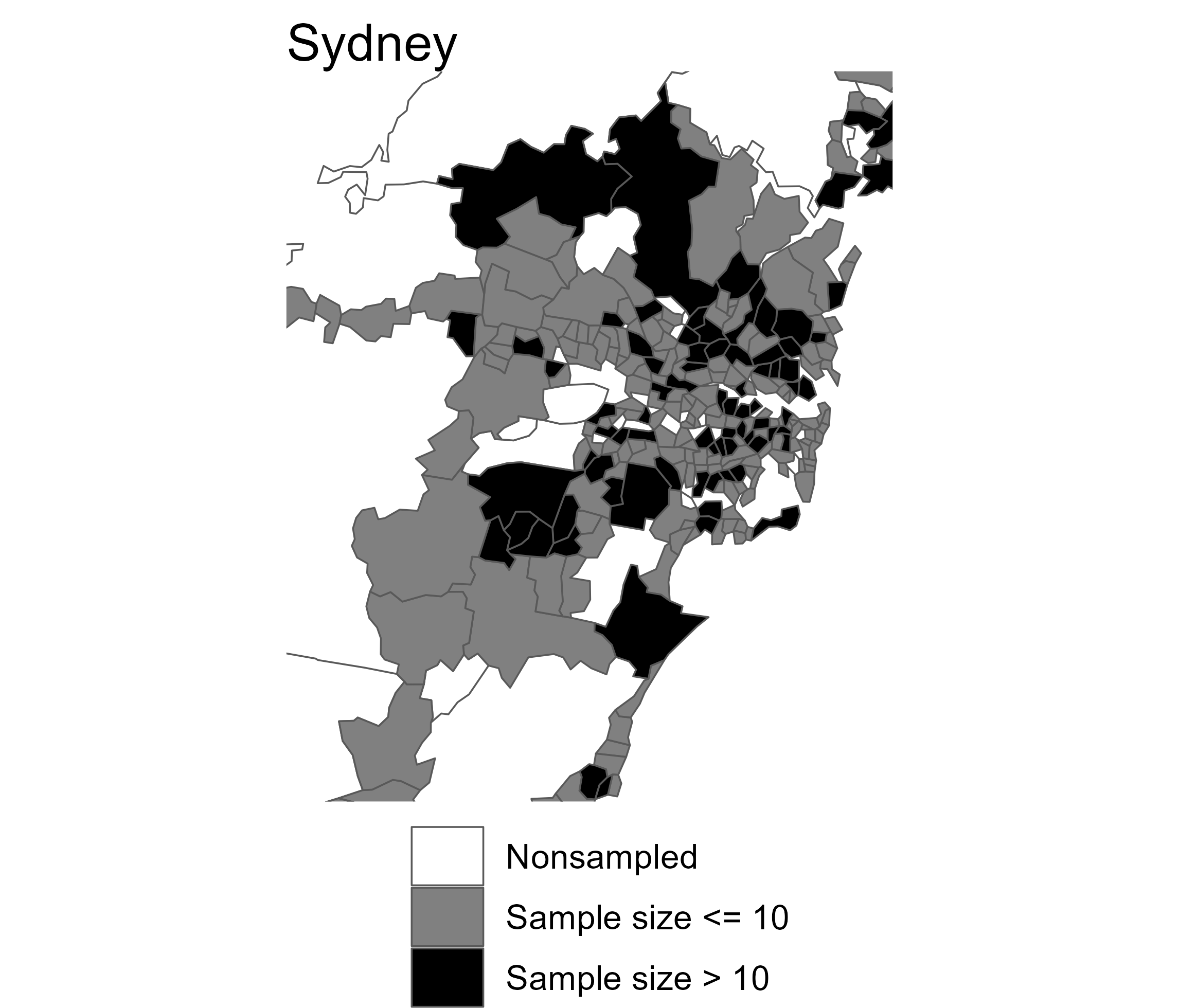
Figure 1: Map of 282 small areas in and around Sydney on the east coast of Australia. Each area is coloured according to the sample size (greater or less than 10) or sample status of the area (sampled or nonsampled) in the 2017-2018 National Health Survey.

The aim of this work is to conceptualize and demonstrate a method for modeling proportions that can provide superior estimates for sparse SAE applications, such as when using the NHS. Our proposed solution, called the two-stage logistic-normal (TSLN) approach, will address the methodological and applied issues described above by using both individual and area level models in a two-stage approach, thus leveraging the strengths of each while mitigating their respective limitations. We adopt a Bayesian perspective and estimate both models using Markov chain Monte Carlo (MCMC) methods [36]. Initially, the TSLN approach stabilizes direct estimates through an individual-level logistic model. Subsequently, it inputs the first stage’s posterior draws into an area-level hierarchical linear model, thereby propagating uncertainty.

The paper is structured as follows. First, we describe the two Bayesian models of our proposed approach and how these link together. Then we describe alternative two-stage and one-stage approaches for proportions. Next, we describe the simulation study conducted to assess the performance of the TSLN approach compared with four alternative models. Finally, we describe a case study where we generated small area level prevalence estimates of current smoking on the east coast of Australia using the 2017-18 NHS.

2 Proposed method

2.1 Notation

We define a finite population where each individual resides in one of $M$ small geographical areas. Allow $N_{i}$ individuals in each area $i=1,\dots,M$, such that $\sum_{i=1}^{M}N_{i}=N$. We are interested in a binary characteristic $y_{ij}\in\{0,1\}$ which is equal to $1$ if individual $j$ in area $i$ has the characteristic and $0$ otherwise. We wish to generate estimates, $\hat{\boldsymbol{\mu}}=\left(\hat{\mu}_{1},\dots,\hat{\mu}_{M}\right)$, of the true proportion of the population with the characteristic, $\boldsymbol{\mu}=\left(\mu_{1},\dots,\mu_{M}\right)$.

Without loss of generality, assume that we have samples from the first $m$ areas, $m<M$, and no samples for the remaining $M-m$ areas. Denote the $n_{i}$ sampled individuals in area $i$ by $j\in r_{i}$ and the $N_{i}-n_{i}$ nonsampled individuals by $j\in r_{i}^{C}$ where $r_{i}^{C}$ is the complement set of $r_{i}$.

Generally, the survey data used in applications of SAE are collected according to a specified survey design. Similar to Vandendijck et al. [33], we assume that in secondary analysis we do not have sufficient details or data to create weights and instead rely on the sampling weights, $w_{ij}^{\text{raw}}$, provided by the data custodians. Using these weights, design-unbiased population estimates can be derived [3].

Throughout this work, $\hat{\mu}_{i}^{D},\hat{\mu}_{i},\mu_{i}$ will denote a direct estimate (using the Hajek [37]), a model-based estimate and the unknown true small area proportion, respectively. Hence,

$$\hat{\mu}_{i}^{D}=\frac{\sum_{j\in r_{i}}w_{ij}y_{ij}}{n_{i}}.$$ (1)

By assuming $w_{ij}=w_{ij}^{\text{raw}}n_{i}\left(\sum_{j\in r_{i}}w_{ij}^{\text{raw}}\right)^{-1}$ and that all the sampling fractions, $n_{i}/N_{i}$, are sufficiently small, we use the following approximation to the sampling variance of the direct proportion estimator [33, 38],

$$\psi_{i}^{D}=\widehat{\text{v}}\left(\hat{\mu}_{i}^{D}\right)=\frac{1}{n_{i}}\left(1-\frac{n_{i}}{N_{i}}\right)\left(\frac{1}{n_{i}-1}\right)$$

$$\sum_{j\in r_{i}}\left(w_{ij}^{2}\left(y_{ij}-\hat{\mu}_{i}^{D}\right)^{2}\right).$$ (2)

Direct estimators have low variance and are design-unbiased for $\mu_{i}$ when $n_{i}$ is large, but high variance when $n_{i}$ is small [39]. Although, model-based methods can be biased, they reduce variance, resulting in lower MSEs [40].

2.2 TSLN approach

The proposed two-stage logistic-normal (TSLN) approach involves two models/stages. In the first stage, an individual level logistic model is fitted to the survey data, where individual level predictions are used to generate area level estimates [41]. In the second stage, these area estimates serve as data in an area level Fay and Herriot [8] (FH) model to further smooth and impute estimates for nonsampled areas [29].

For the sake of clarity, we describe and investigate our approach in its most generalized form, encompassing both individual and area level models of a similarly generic nature. It is worth noting that more sophisticated modeling techniques — such as non-linear regression or spatial smoothing [42, 43] — are not only feasible but also advisable. Moreover, benchmarking approaches [44, 45] could be utilized after fitting the stage 2 model or incorporated directly into the stage 2 model using fully Bayesian benchmarking [46]. We employ some of these sophisticated modeling techniques in Section 5.

2.2.1 Stage 1

The goal of the stage 1 model is to stabilize the area level direct estimates and sampling variances whilst simultaneously reducing their bias and accommodating the sample design. This is achieved by fitting a Bayesian logistic mixed model to the individual level binary outcomes, $y_{ij}$.

For design-consistent estimation of the model parameters we use pseudo-likelihood, which can be described as the Horvitz-Thompson estimator of the population-level log-likelihood [47, 48] (see Supplemental Materials B [49]). Following the notation of Parker et al. [34, 50], we represent the pseudo-likelihood for a probability density function, $p(.)$, as $p(y_{ij})^{\tilde{w}_{ij}}$, where $\tilde{w}_{ij}$ are the sample scaled weights, $\tilde{w}_{ij}=w_{ij}^{\text{raw}}n\left(\sum_{i=1}^{m}\sum_{j=1}^{n_{i}}w_{ij}^{\text{raw}}\right)^{-1}$. The rescaling of the weights is recommended by Savitsky and Toth [48] in their work on Bayesian pseudo-likelihoods.

The stage 1 model, similar to Model 1 in Parker et al. [34], is,

$$y_{ij} \sim \text{Bernoulli}(p_{ij})^{\tilde{w}_{ij}}$$ (3)

$$\text{logit}(p_{ij}) = \mathbf{x}_{ij}\boldsymbol{\beta}+e_{i}$$

$$e_{i} \sim N(0,\sigma_{e}^{2})$$

where $j=1,\dots,n_{i};i=1,\dots,m$. In (3), $\mathbf{x}$ is the design matrix, which includes the fixed effects (individual level survey-only and area level fixed effects), and $\boldsymbol{\beta}$ the corresponding regression coefficients.

Noninformative and diffuse priors (e.g. $\boldsymbol{\beta}\propto 1$ and $\sigma_{e}\propto 1$) are common choices in Bayesian SAE [3, 51]. Recently however, weakly informative priors, which consider the scale of the data, are preferred to these flat priors [52]. We used $N(0,2)$ priors for the fixed regression coefficients $\boldsymbol{\beta}$ and a student-$t(df=3,\mu=0,\sigma=1)$ prior for the intercept (implied in $\mathbf{x}_{ij}\boldsymbol{\beta}$). A weakly informative $N(0,1)^{+}$ prior was used for $\sigma_{e}$.

The stage 1 model will be referred to as the TSLN-S1 model hereafter.

2.2.2 Stage 1 (S1) estimates

To derive area level estimates suitable for area level modeling, we collapse the individual level data to area level data by calculating S1 proportion estimates, $\hat{\mu}_{i}^{\text{S1}}$, and their corresponding sampling variances, $\psi_{i}^{\text{S1}}$. These values are derived using the posterior distributions for the individual level probabilities, $p_{ij}$ instead of the observed binary outcomes, $y_{ij}$.

Smoothing the individual level data in this way, which is similar to the work by Gao and Wakefield [53], permits one to view the TSLN-S1 model as a model-based smoothing method. However, unlike their work [29], the S1 estimates are aggregates of the sampled individuals only. This highlights the distinction between our proposed approach and the model-assisted framework [54]. Note that using S1 estimates guarantees that the values are stable: all $\hat{\mu}_{i}^{\text{S1}}\in(0,1)$ and $\psi_{i}^{\text{S1}}>0$.

To accommodate the uncertainty of the TSLN-S1 model, we approximate the posterior distribution for the S1 estimates. To do so, all the steps to aggregate the individual level predictions are done for each posterior draw, which are indexed by $t=1,\dots,T$.

The S1 estimate for area $i$ and posterior draw $t$ is,

$$\hat{\mu}^{\text{S1},t}_{i} = \frac{\sum_{j\in r_{i}}w_{ij}p_{ij}^{t}}{n_{i}}$$ (4)

$$\psi_{i}^{\text{S1},t} = \widehat{\text{v}}\left(\hat{\mu}^{\text{S1},t}_{i}\right)=\widehat{\text{v}}\left(\hat{\mu}^{D}_{i}\right)+\widehat{\text{v}}\left(\hat{B}_{i}^{t}\right)$$ (5)

$$\hat{B}_{i}^{t} = \frac{\sum_{j\in r_{i}}w_{ij}\left(p_{ij}^{t}-y_{ij}\right)}{n_{i}}$$ (6)

where $\hat{B}_{i}^{t}$ quantifies the level of smoothing achieved by using the TSLN-S1 model (See Supplemental Materials A [49] for details). The formula used to calculate both $\widehat{\text{v}}\left(.\right)$ terms is given in (2).

To accommodate the constraints on the S1 estimates in the stage 2 model, we use the common empirical logistic transformation [18, 38],

$$\hat{\theta}_{i}^{\text{S1},t} = \text{logit}\left(\hat{\mu}_{i}^{\text{S1},t}\right)$$ (7)

$$\gamma_{i}^{\text{S1},t} = \psi_{i}^{\text{S1},t}\left[\hat{\mu}_{i}^{\text{S1},t}\left(1-\hat{\mu}_{i}^{\text{S1},t}\right)\right]^{-2}$$ (8)

where $\hat{\theta}_{i}^{\text{S1},t}$ is the log-odds of the S1 estimate and $\gamma_{i}^{\text{S1},t}$ the corresponding sampling variance for area $i$ and posterior draw $t$. The logistic transformation permits the use of a Gaussian likelihood in the stage 2 model, which improves computation and avoids the limitations of the Beta distribution (see Supplemental Materials B [49]).

2.2.3 Assessing smoothing properties

Whilst multi-stage or double smoothing of survey data has been shown to provide optimal predictive performance [29, 30], the degree of smoothing should be monitored. Predictions from the TSLN-S1 model should provide acceptable approximations to the observed values, whilst still ensuring a level of generalisability. Severely overfit TSLN-S1 models will yield minimal smoothing and stability gains, while poor-fitting models can exhibit very high sampling variances, biased S1 estimates and inaccurate estimates for nonsampled areas. Therefore, the stability gained from smoothing the individual level data must be balanced by ensuring adequate agreement (and comparable variability) of the S1 and direct estimates.

To assess the level of agreement, we regress the posterior median of $\left(\hat{\theta}_{i}^{\text{S1},t},\dots,\hat{\theta}_{i}^{\text{S1},T}\right)$ on $\hat{\theta}_{i}^{D}$ with weights $\frac{1}{\psi_{i}^{D}}$. The estimated slope from this regression is defined as the area linear comparison (ALC), with values closer to 1 indicating less smoothing and more agreement between the S1 and direct estimates.

We are yet to provide a theoretical threshold for when the ALC measure may indicate over-smoothing. However, the simulation study described in Supplemental Materials E suggested that optimal performance could be achieved approximately when $0.55<ALC<0.75$, with performance atrophy outside these bounds. We found that values at the lower end of these bounds generally provided narrower and more reliable uncertainty intervals.

2.2.4 Stage 2

To accommodate the posterior draws from the stage 1 model, we derive the following summaries of the S1 estimates. Let $\bar{\gamma}_{i}^{\text{S1}}$ be the empirical mean of $\left(\gamma_{i}^{\text{S1},1:T}\right)$, $\widehat{\text{v}}\left(\hat{\theta}_{i}^{\text{S1}}\right)$ be the empirical variance of $\left(\hat{\theta}_{i}^{\text{S1},1:T}\right)$ and $\hat{\boldsymbol{\theta}}_{i}^{\text{S1}}$ be a random subset from $\left(\hat{\theta}_{i}^{\text{S1},1:T}\right)$ of size $\widetilde{T}$. We use a random subset to reduce the computational burden, whilst simultaneously accommodating the uncertainty of the stage 1 model. In this work we use $\widetilde{T}=T/2$ (i.e. 50% of the posterior draws). A more detailed description and some alternative approaches to accommodate the uncertainty of the stage 1 model are given in Supplemental Materials A [49].

The stage 2 model, referred to as the TSLN-S2 model hereafter, is composed of: a measurement error model [55],

$$\hat{\boldsymbol{\theta}}_{i}^{\text{S1}}\sim N\left(\hat{\bar{\theta}}_{i},\widehat{\text{v}}\left(\hat{\theta}_{i}^{\text{S1}}\right)\right),$$ (9)

which accommodates some of the uncertainty of the stage 1 model; a sampling model,

$$\hat{\bar{\theta}}_{i}\sim N\left(\hat{\theta}_{i},\bar{\gamma}_{i}^{\text{S1}}\right),$$ (10)

which accommodates the sampling variance; and a linking model,

$$\hat{\theta}_{i} = \mathbf{Z}_{i}\boldsymbol{\lambda}+v_{i}$$ (11)

$$v_{i} \sim N(0,\sigma_{v}^{2}),$$

which relates the modeled values, $\hat{\theta}_{i}$, to a series of covariates and area level random effects $\mathbf{v}=\left(v_{1},\dots,v_{M}\right)$ for $i=1,\dots,M$. We used $N(0,2)$ priors for the fixed regression coefficients $\boldsymbol{\lambda}$ and a student-$t(df=3,\mu=0,\sigma=1)$ prior for the intercept (implied in $\mathbf{Z}_{i}\boldsymbol{\lambda}$). A weakly informative $N(0,2)^{+}$ prior was used for $\sigma_{v}$.

Note that $\mathbf{Z}$ is the design matrix, which should include area level covariates that are available for all $M$ areas, and $\boldsymbol{\lambda}$ is the corresponding regression coefficients. Although S1 estimates are not available for areas $m+1,\dots,M$, Tzavidis et al. [56] show how estimates can be obtained by combining the areas’ known covariate values (i.e. $\mathbf{Z}$) and random draws from the priors. To ensure that posterior uncertainty remains unaffected by the choice of $\widetilde{T}$, we downscale the likelihood contribution in (9) by $1/\widetilde{T}$.

The parameter of interest (i.e. proportion) is the posterior distribution of $\hat{\mu}_{i}=\text{logit}^{-1}(\hat{\theta}_{i})$, which can be described by deriving summary quantities (such as means, variances and highest density intervals) of the posterior draws of $\hat{\mu}_{i}$ [57, 39, 3].

2.2.5 Generalized variance functions (GVF)

FH models require valid direct estimates and sampling variances for all sampled areas. As discussed previously, for very sparse survey data, many sampled areas may give unstable estimates ($\hat{\mu}_{i}^{D}=0$ or $1$) and thus sampling variances that are highly fluctuating, undefined or exactly zero. The reader is reminded that an area is defined as unstable according to its direct estimate only.

The stage 1 model provides more consistent area level estimates and sampling variances, reducing the need for pre-smoothing, a standard practice in area level modeling [3, 58]. That said, S1 sampling variances do exhibit undesirable limit properties. This is because they are derived from probabilities rather than binary random variables. For example, consider a single area $i$ with a sample size of 4 and assume that $w_{ij}=1,\forall j$. While it is possible for $\hat{\mu}^{\text{S1}}_{i}=0.01$, to obtain $\hat{\mu}^{D}_{i}=0.01$ one would require 25 times the sample size. In other words, for a fixed sample size, S1 estimates are able to be much closer to zero (or one), without being exactly zero (or one), than direct estimates. The result of this phenomenon is unrealistically low S1 sampling variances for unstable areas.

Our solution is to use generalized variance functions (GVF), which relate the sampling variance of a direct estimate to a set of covariates, often including the sample sizes and direct estimates, with necessary transformations [15, 3, 58]. To ensure that S1 sampling variances for unstable areas do not inadvertently affect the fit of the FH model in (10), we impute the $m-m_{s}$ S1 sampling variances using GVF, where $m_{s}<m<M$ is the number of stable areas.

In this work, we generalize the approach used by Das et al. [30] to a fully Bayesian framework by implementing the GVF within our model. By fitting the GVF and stage 2 model jointly [53] we ensure the uncertainty of the imputations is appropriately taken into account.

Unlike standard practice where GVFs are applied to all direct sampling variances [3, 58], our approach only requires this for unstable areas. We use the stable S1 sampling variances, $\bar{\gamma}_{i}^{\text{S1}}$, to estimate the parameters of the GVF and then use the fitted GVF to impute the S1 sampling variances for the unstable areas only. Note that S1 sampling variances were not imputed for non-sampled areas. For more details on the GVF used in this work, see Supplemental Materials A [49].

3 Existing methods

Name	Model	Limitations	Reference
Logistic model (LOG)	$\displaystyle y_{ij}$ $\displaystyle\sim$ $\displaystyle\text{Bernoulli}(p_{ij})^{\tilde{w}_{ij}}\quad\quad j=1,\dots,n_{i};i=1,\dots,m$ $\displaystyle\text{logit}(p_{ij})$ $\displaystyle=$ $\displaystyle\mathbf{x}_{ij}\boldsymbol{\beta}+e_{i}\quad\quad j=1,\dots,N_{i};i=1,\dots,M$ $\displaystyle\hat{\mu}_{i}$ $\displaystyle=$ $\displaystyle\frac{1}{N_{i}}\sum_{j=1}^{N_{i}}p_{ij}\quad\quad i=1,\dots,M$	Requires access to covariate data for the entire population	[48, 34]
Binomial model (BIN)	$\displaystyle\sum_{j\in r_{i}}y_{ij}$ $\displaystyle\sim$ $\displaystyle\text{Binomial}(n_{i},\hat{\mu}_{i})\quad\quad i=1,\dots,m$ $\displaystyle\text{logit}(\hat{\mu}_{i})$ $\displaystyle=$ $\displaystyle\mathbf{Z}_{i}\boldsymbol{\lambda}+v_{i}\quad\quad i=1,\dots,M$	Does not accommodate sample design	[10, 59]
Beta model (BETA)	$\displaystyle\hat{\mu}^{D}_{i}$ $\displaystyle\sim$ $\displaystyle\text{Beta}\left(\hat{\mu}_{i}\phi_{i},\phi_{i}-\hat{\mu}_{i}\phi_{i}\right)\quad\quad i=1,\dots,m$ $\displaystyle\phi_{i}$ $\displaystyle=$ $\displaystyle\frac{\hat{\mu}_{i}(1-\hat{\mu}_{i})}{\psi^{D}_{i}}-1\quad\quad i=1,\dots,m$ $\displaystyle\text{logit}(\hat{\mu}_{i})$ $\displaystyle=$ $\displaystyle\mathbf{Z}_{i}\boldsymbol{\lambda}+v_{i}\quad\quad i=1,\dots,M$	Requires $\hat{\mu}_{i}^{D}\in(0,1)$ and $\psi^{D}_{i}\in(0,0.25)$, $\forall i$ Possible bimodal posterior Requires GVFs for unstable and missing areas Areas with very large $\psi^{D}_{i}$, give $\hat{\mu}_{i}$ values close to 0.5	[12, 13]
Empirical-logistic normal model (ELN)	$\displaystyle\text{logit}\left(\hat{\mu}_{i}^{D}\right)$ $\displaystyle\sim$ $\displaystyle N\left(\text{logit}\left(\hat{\mu}_{i}\right),\gamma_{i}^{D}\right)\quad\quad i=1,\dots,m$ $\displaystyle\gamma_{i}^{D}$ $\displaystyle=$ $\displaystyle\psi_{i}^{D}\left[\hat{\mu}_{i}^{D}\left(1-\hat{\mu}_{i}^{D}\right)\right]^{-2}\quad\quad i=1,\dots,m$ $\displaystyle\text{logit}\left(\hat{\mu}_{i}\right)$ $\displaystyle=$ $\displaystyle\mathbf{Z}_{i}\boldsymbol{\lambda}+v_{i}\quad\quad i=1,\dots,M$	Requires $\hat{\mu}_{i}^{D}\in(0,1)$, $\forall i$ Requires GVFs for unstable areas	[18, 38, 13]

Table 1: Description of the individual and area level comparison models with their corresponding model identifiers (e.g. ELN, LOG, etc). Model details can be found in both Section 3.2 and Supplemental Materials B [49], while generalized variance functions (GVFs) are described in Section 2.2.5. Note that $e_{i}\sim N(0,\sigma_{e}^{2})$ and $v_{i}\sim N(0,\sigma_{v}^{2})$ and weakly informative priors are used for the remaining parameters (see Sections 2.2.1, 2.2.4 and 4).

3.1 Two-stage approaches

Our two-stage approach builds on the similar intuition of Gao and Wakefield [29] (hereafter named the GW model) and Das et al. [30], but with several improvements. Firstly, unlike previous approaches that treat predictions from the first stage as fixed, the TSLN-S2 model accommodates the uncertainty in the model parameters and predictions from the TSLN-S1 model. Gao and Wakefield [29] warn against overconfident estimates, as their stage 1 LGREG estimator, fit using frequentist inference, ignores model parameter uncertainty. By using Bayesian inference at both the individual and area level, our estimates inherit the uncertainty from model fitting.

Secondly, our approach relaxes some covariate requirements. While the GW model assumes that the stage 1 model provides “unbiased” predictions for all individuals and areas this assumption can be restrictive. Specifically, the GW model requires individual-level covariates for all population individuals and prohibits the use of survey-only covariates. Fortunately, the TSLN approach has no such requirement or prohibition. Note that Gao and Wakefield [29] acknowledge the limitations of requiring access to covariate information for the entire population. Their solution involved redefining individuals as very fine spatial grids, for which population data were available.

Thirdly, the GW approach requires access to first and second-order inclusion probabilities in order to calculate the sampling variance of their first stage LGREG estimates. In most cases, first-order inclusion probabilities are not provided by data custodians, and further, it is very rare to have access to second-order probabilities. Our TSLN approach only assumes access to sample weights, which are typically provided with survey data. Finally, unlike the model of Das et al. [30], which operates solely at the area level, the TSLN approach can provide more efficient estimates by smoothing the data at both the individual and area levels.

Note that we do not use the GW model as a comparison model in Section 4 as it uses a frequentist approach for the stage 1 model and requires pairwise sampling probabilities which we assume are inaccessible. Nor do we compare our approach to that of Das et al. [30] model as it requires temporal data.

3.2 Models for proportions

As with the TSLN approach, those developed by Gao and Wakefield [29] and Das et al. [30] are composed of basic component models such as the logistic and FH. Table 1 gives an overview of four different model-based techniques for small area estimation of proportions that serve as comparison models in the simulation experiment described in Section 4. However, now we briefly address some of the challenges and limitations of these and other alternative methodologies (see Supplemental Materials B [49] for more details), as well as how the TSLN approach offers some solutions. In addition, we provide justification for the four comparison models used in this work.

BIN model Despite their common use [3], standard FH models are generally not suitable to model sparse binary data due to unstable direct estimates. Instability is alleviated by considering an aggregation of the binary outcomes via a binomial model. However, these models do not generally accommodate the sampling methodology. In contrast, our approach provides stable direct estimates and accommodates the survey design. In this study, we deliberately selected a binomial model that ignores the sampling methodology as a baseline (crude) model against which the TSLN approach was evaluated in terms of design consistency.

BETA model Although the Beta distribution is a natural choice when modeling proportions [60, 11, 12, 13], it has several statistical and computational limitations that arise when modeling sparse survey data (see Table 1 and Supplemental Materials B [49]). These include: problematic constraints on the $\hat{\mu}_{i}$’s which depend on the $\psi^{D}_{i}$’s; the necessity to impute sampling variances for non-sampled areas; bimodal behaviour which causes significant MCMC convergence issues; and undefined likelihoods for unstable direct estimates. Nevertheless, the FH Beta model is a popular solution for modeling proportions [13]; thus, it was chosen as one of the comparison models.

ELN model Other area level models for proportions assume Gaussian distributions for the direct estimates, allowing the use of typical FH models [11]. Although this method is effective for applications with large area sample sizes, in the situation of sparsity, the Gaussian approximation proves insufficient [13]. Instead, researchers use the empirical logistic transformation before using an FH model. This is the technique used by Mercer et al. [18] and Cassy et al. [38], and by us. Liu et al. [13] present a similar model (Model 3), which utilizes the design effect to compute sampling variances. Since the ELN model is most similar to ours, we included it in our comparisons to evaluate the advantages of using S1 over direct estimates.

LOG model Individual level models for binary data offer significant advantages over the area level models discussed above. Most notably, working at the individual level eliminates the need for direct estimates, and allows for greater model flexibility. However, these models require covariate data for all persons in the population [20, 21], which is often sourced from census microdata. This introduces further restrictions on covariate choice due to the necessary concordance between survey and census covariates. Covariates collected in a census may be less predictive of health-related outcomes, whilst individual level survey-only covariates may be more useful. The TSLN-S1 model does not predict values for the whole population, hence easing the requirement for survey-census concordance and permitting the inclusion of survey-only covariates.

Another limitation of individual level models is that they do not accommodate known sample weights and are susceptible to bias under informative sampling. A simple solution is to include the sample weights as covariates, but this requires imputation for nonsampled individuals [33]. Bayesian pseudo-likelihood [47] is an alternative used by Parker et al. [34, 50] (see Supplemental Materials B [49]). By construction, our TSLN approach accommodates the sample design at both stages; pseudo-likelihood in (3) and the weighted estimators in (4). Comparing our TSLN approach to a pseudo-likelihood LOG model (similar to MrP [24, 25, 20]) enables us to assess the effectiveness of utilizing survey-only covariates and the utility of two-stage methods in general.

4 Simulation Study

To evaluate the performance of the TSLN approach, we undertook a simulation experiment based on the approach used by Buttice and Highton [61]. In contrast to conventional simulation studies where data are generated directly from the target model, the two-stage structure of our approach required a reverse method. We generated a census by first simulating the area level proportions and then generating individual and area level covariates based on these, implicitly allowing for specified levels of association and random effects. For simplicity, no spatial autocorrelation was imposed between areas. From the fixed census, we repeatedly drew unique surveys using a multi-stage informative design.

First, we generated individual level census data for $100$ small areas with populations ranging from $500$ and $3000$. The simulated census included the binary outcomes, $\mathbf{y}$, two individual-level covariates (one survey-only categorical covariate, $\mathbf{x}^{\text{survey}}$ with three groups, and one continuous covariate, $\mathbf{x}^{\text{census}}$ available in both the census and survey) and a single area level covariate ($\mathbf{Z}$). To explore how the association of the survey-only covariate affected the overall performance of our approach, we used two levels; high and average (see Table 2).

Keeping the census, and thus true proportions, fixed, we then drew 500 unique (repetitions) surveys, fitting the TSLN and four comparison models (Table 1) to each. We used a sampling fraction of 0.4% and only sampled $60$ areas for each repetition. Following Hidiroglou and You [58], we devised the sampling method so that individuals with a binary value of 0 were more likely to be sampled and constructed sample weights to reflect this. Extensive details of the simulation algorithm can be found in Supplemental Materials C [49].

The median sample size, $n$, population size, $N$, and area sample size, $n_{i}$ were 771, 177263, and 8 respectively. Note that it is relatively rare for simulation experiments in the SAE literature to use such small area level sample sizes; generally $n_{i}>50$ [29, 62, 34, 63], which is less relevant in the Australian context. Unstable direct estimates for all comparison models were stabilized via the simple perturbation method [13]; add or subtract a value of $0.001$ to any $\hat{\mu}_{i}^{D}=0$ or $1$, respectively, prior to modeling.

Overall, we wished to explore how the TSLN approach performed for sparse survey data. In addition, we wanted to assess performance for varying degrees of prevalence and for the inclusion of more predictive individual level survey-only covariates. These objectives translated to the six simulation scenarios given in Table 2. Note that Sc1, Sc3, and Sc5 ensure that the survey-only covariate is much more predictive of the outcome than the census-available covariate. Given the informative sample design, the rare scenarios (Sc3 and Sc4) will provide a high number of unstable direct estimates (see Table 4).

		Predictive $\mathbf{x}^{\text{survey}}$	$L$	$U$
50-50	Sc1	High	0.35	0.65
	Sc2	Average
Rare	Sc3	High	0.1	0.4
	Sc4	Average
Common	Sc5	High	0.6	0.9
	Sc6	Average

Table 2: Summary of the six simulation scenarios. $L$ and $U$ give the lower and upper bounds of the true proportions, respectively (see Supplemental Materials C [49] for more details).

As described in Section 3 we compared the performance of our approach to the four model-based SAE methods summarized in Table 1. Both models of the TSLN approach and the BETA, LOG and ELN models were fit using rstan, leveraging Hamiltonian Monte Carlo (HMC) [64]. The BIN model was fit using JAGS via rjags [65]. The covariates used in the models are given in Table 3. Only models deemed to have converged were used in the simulation results. Convergence was assessed using $\widehat{R}$ [66]. Any analysis for which at least one parameter of interest had $\widehat{R}>1.02$ was discarded. We used $2,000$ post-warmup and $6,000$ post-burnin draws for each of four chains for the Stan and JAGS models, respectively. R code to run the simulations, with the necessary Stan and JAGS code is available here.

		$\mathbf{x}^{\text{survey}}$	$\mathbf{x}^{\text{census}}$	$\mathbf{Z}$
Individual level	TSLN-S1	✓	✓	✓
	LOG		✓	✓
Area level	TSLN-S2			✓
	ELN			✓
	BETA			✓
	BIN			✓

Table 3: Illustrates which of the simulated covariates, described in Section 4, were used in which models in the simulation study. Ticks denote that the model specified in the row used the covariate (shown in the column) as a fixed effect. The estimated regression coefficients and variance terms varied across models, scenarios and repetitions (see Supplemental Materials C [49]).

Similar to the TSLN approach, all fixed regression parameters in the comparison models were given a $N(0,2)$ prior, whilst intercept terms were given a student-$t(df=3,\mu=0,\sigma=1)$ prior. Standard deviation parameters in the TSLN-S1, LOG and BIN models were given a weakly informative $N(0,1)^{+}$ prior, while standard deviation parameters in the BETA, ELN and TSLN-S2 models were given a $N(0,2)^{+}$ prior. Note that the GVF described in Section 2.2.5 was necessarily adjusted for the Beta model (See Supplemental Materials B [49] for details). All design matrices were mean-centered prior to model fitting and the popular QR decomposition was used [67].

4.1 Performance metrics

To compare the models we use Bayesian performance metrics which are calculated separately depending on whether an area was sampled or nonsampled in repetition $d$. Unlike common frequentist metrics (see Supplemental Materials C [49]), Bayesian metrics use all the appropriate posterior samples during calculation. Thus, they generally favor posteriors with smaller variance, whilst still penalizing inaccuracy. While Bayesian coverage is summed over all areas and repetitions, the remaining metrics are calculated independently for each repetition, $d$. The simulations provide $500\times T$ posterior draws for each area, model and scenario. Let $\hat{\mu}_{idt}$ be the $t$th posterior draw for repeat $d$ in area $i$ and $\mu_{i}$ be the true proportion in area $i$. Also let $\hat{\mu}_{id}^{\text{(L)}}$ and $\hat{\mu}_{id}^{\text{(U)}}$ denote the lower and upper bounds, respectively, of the posterior 95% highest density interval (HDI) for area $i$ and repeat $d$.
Absolute relative bias: ARB_id

$$\left|\frac{\frac{1}{T}\sum_{t=1}^{T}\left(\hat{\mu}_{idt}-\mu_{i}\right)}{\mu_{i}}\right|$$ (12)

Relative root mean square error: RRMSE_id

$$\frac{\sqrt{\frac{1}{T}\sum_{t=1}^{T}\left(\hat{\mu}_{idt}-\mu_{i}\right)^{2}}}{\mu_{i}}$$ (13)

Coverage

$$\frac{1}{MD}\sum_{i=1}^{M}\sum_{d=1}^{D}\mathbb{I}\left(\hat{\mu}_{id}^{\text{(L)}}<\mu_{i}<\hat{\mu}_{id}^{\text{(U)}}\right)$$ (14)

We take the mean across all areas to derive the mean RRMSE (MRRMSE) and mean ARB (MARB) for each repetition. While the distribution of these 500 MRRMSE and MARB values are visualized in Fig. 2 and 3, respectively, summaries are given in Table 5.

4.2 Results

		Percent of sampled areas unstable (%)	ALC	Percent increase in sampling variance (%)	Percent reduction in MAB (%)
50-50	Sc1	3.3 (1.7, 5.0)	0.69 (0.66, 0.73)	56 (27, 91)	25 (22, 28)
	Sc2	3.3 (1.7, 5.0)	0.65 (0.60, 0.68)	74 (40, 107)	30 (27, 34)
Rare	Sc3	25.0 (21.7, 28.3)	0.78 (0.73, 0.82)	79 (36, 140)	24 (21, 28)
	Sc4	25.0 (21.7, 28.3)	0.76 (0.71, 0.80)	101 (53, 162)	27 (24, 31)
Common	Sc5	1.7 (0.0, 3.3)	0.66 (0.62, 0.70)	66 (29, 108)	30 (26, 34)
	Sc6	1.7 (0.0, 3.3)	0.59 (0.55, 0.64)	79 (36, 123)	38 (34, 42)

Table 4: Overview of the simulation and smoothing properties of the TSLN-S1 model (see Supplemental Materials C [49]), including the area linear comparison (ALC) metric (Section 2.2.3), and mean absolute bias (MAB) along with the interquartile bounds in brackets. Column one is derived by calculating the percentage of sampled areas with unstable direct estimates for each repetition, before taking the median (and IQ bounds) of these 500 percentages. Column two is derived by taking the median (and IQ bounds) of the 500 ALC values. The third column is derived by first calculating the median of the area-specific ratios of the stage 1 sampling variances to the direct sampling variances for each repetition, before taking the median (and IQ bounds) of the 500 values (details are given in Supplemental Materials C [49]). Large values indicate large increases in the S1 sampling variances above that of the direct, which is undesirable. The final column is derived by first calculating the ratio between the MABs for the direct and S1 estimates for each repetition, before taking the median (and IQ bounds) of these 500 ratios (details are given in Supplemental Materials C [49]). Large values indicate larger reductions in MAB when using the S1 estimates, which is preferable.

			Sampled areas				Nonsampled areas
			MRRMSE	MARB	CI width	Coverage	MRRMSE	MARB	CI width	Coverage
50-50	Sc1	BETA	0.36 (2.17)	0.22 (1.96)	0.46	0.80	0.40 (2.29)	0.16 (1.35)	0.61	1.00
		BIN	0.39 (2.38)	0.38 (3.35)	0.18	0.03	0.40 (2.30)	0.38 (3.29)	0.20	0.03
		ELN	0.34 (2.08)	0.21 (1.84)	0.43	0.91	0.40 (2.32)	0.15 (1.32)	0.64	1.00
		LOG	0.25 (1.52)	0.16 (1.41)	0.32	0.90	0.28 (1.61)	0.10 (0.83)	0.47	1.00
		TSLN	0.17 (1.00)	0.11 (1.00)	0.22	0.94	0.17 (1.00)	0.12 (1.00)	0.23	0.95
	Sc2	BETA	0.36 (2.13)	0.22 (1.90)	0.46	0.80	0.40 (2.25)	0.16 (1.29)	0.62	1.00
		BIN	0.39 (2.33)	0.38 (3.25)	0.18	0.03	0.40 (2.26)	0.38 (3.17)	0.20	0.03
		ELN	0.34 (2.04)	0.21 (1.79)	0.43	0.91	0.40 (2.29)	0.15 (1.26)	0.64	1.00
		LOG	0.25 (1.49)	0.16 (1.37)	0.32	0.90	0.28 (1.58)	0.10 (0.80)	0.47	1.00
		TSLN	0.17 (1.00)	0.12 (1.00)	0.22	0.93	0.18 (1.00)	0.12 (1.00)	0.23	0.95
Rare	Sc3	BETA	0.47 (1.46)	0.31 (1.39)	0.21	0.66	0.51 (1.57)	0.22 (1.08)	0.34	0.97
		BIN	0.50 (1.54)	0.48 (2.16)	0.12	0.08	0.50 (1.54)	0.47 (2.29)	0.13	0.08
		ELN	0.78 (2.42)	0.55 (2.52)	0.39	0.68	1.03 (3.17)	0.20 (0.96)	0.77	1.00
		LOG	0.50 (1.55)	0.35 (1.60)	0.28	0.82	0.55 (1.68)	0.15 (0.73)	0.43	1.00
		TSLN	0.32 (1.00)	0.22 (1.00)	0.19	0.86	0.32 (1.00)	0.21 (1.00)	0.20	0.88
	Sc4	BETA	0.47 (1.43)	0.31 (1.36)	0.21	0.66	0.50 (1.54)	0.22 (1.03)	0.34	0.97
		BIN	0.50 (1.51)	0.48 (2.10)	0.12	0.09	0.50 (1.53)	0.47 (2.18)	0.14	0.09
		ELN	0.78 (2.38)	0.55 (2.44)	0.39	0.68	1.02 (3.12)	0.20 (0.92)	0.77	1.00
		LOG	0.50 (1.52)	0.35 (1.55)	0.28	0.82	0.54 (1.66)	0.15 (0.70)	0.43	1.00
		TSLN	0.33 (1.00)	0.23 (1.00)	0.19	0.86	0.33 (1.00)	0.22 (1.00)	0.19	0.88
Common	Sc5	BETA	0.16 (2.01)	0.09 (1.76)	0.31	0.89	0.18 (2.25)	0.04 (0.87)	0.43	1.00
		BIN	0.25 (3.13)	0.24 (4.80)	0.19	0.05	0.25 (3.04)	0.23 (4.64)	0.21	0.08
		ELN	0.12 (1.52)	0.07 (1.37)	0.26	0.98	0.13 (1.58)	0.06 (1.18)	0.31	1.00
		LOG	0.11 (1.40)	0.06 (1.28)	0.24	0.97	0.12 (1.45)	0.05 (0.99)	0.29	1.00
		TSLN	0.08 (1.00)	0.05 (1.00)	0.16	0.98	0.08 (1.00)	0.05 (1.00)	0.17	0.99
	Sc6	BETA	0.16 (2.02)	0.09 (1.81)	0.31	0.89	0.18 (2.26)	0.04 (0.88)	0.43	1.00
		BIN	0.25 (3.15)	0.24 (4.96)	0.19	0.05	0.25 (3.05)	0.23 (4.78)	0.21	0.08
		ELN	0.12 (1.53)	0.07 (1.41)	0.26	0.98	0.13 (1.58)	0.06 (1.20)	0.31	1.00
		LOG	0.11 (1.43)	0.06 (1.32)	0.24	0.97	0.12 (1.47)	0.05 (1.02)	0.30	1.00
		TSLN	0.08 (1.00)	0.05 (1.00)	0.16	0.98	0.08 (1.00)	0.05 (1.00)	0.16	0.98

Table 5: Median of the 500 MRRMSE and MARB values. The table also includes the width of 95% posterior credible interval (CI width) and coverage across the 500 repetitions. Bold numbers represent the lowest value in each column, scenario and whether the metric is for sampled or nonsampled areas. For coverage, bold numbers denote the value closest to 0.95. Gray numbers in brackets give the ratio of the value to that of the TSLN approach.

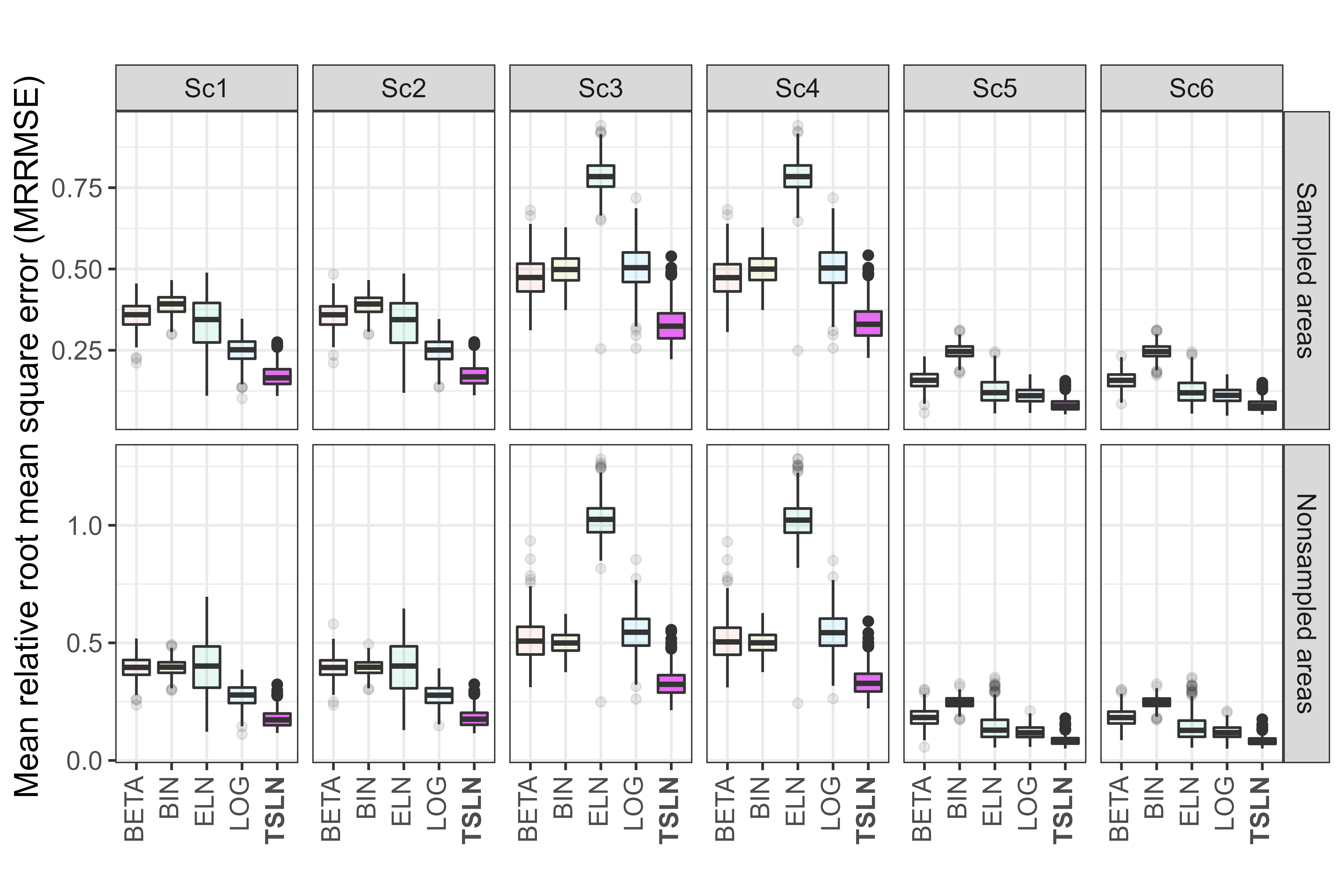
Figure 2: Boxplots of the 500 MRRMSE values. The medians of each boxplot are available in Table 5.

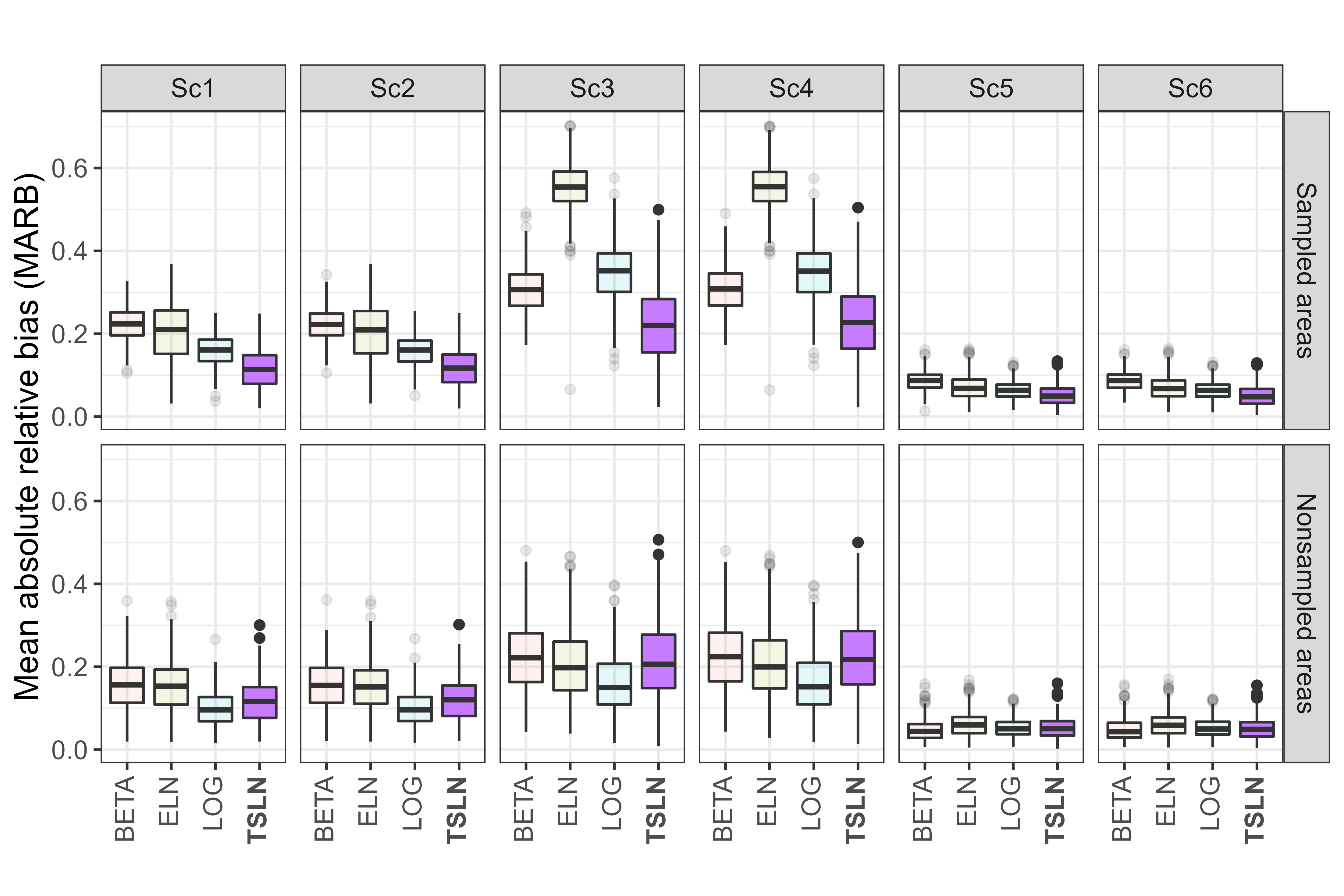
Figure 3: Boxplots of the 500 MARB values. The medians of each boxplot are available in Table 5. We have omitted the BIN model; its very large bias distorts the plot.

4.2.1 Stage 1 results

Table 4 summarises the simulated data and provides details on the smoothing properties of the TSLN-S1 model. As anticipated with more predictive individual level covariates (e.g. Sc1 versus Sc2), the ALC is closer to 1. However, the differences are subtle. The biggest effect of having more predictive individual level covariates is the significantly smaller increase in sampling variance. However, this comes at the cost of a lower reduction in the mean absolute bias between the S1 or direct estimates and the true values. This pattern is expected because the S1 estimates will collapse to the direct estimates when the TSLN-S1 model “overfits” the survey data.

4.2.2 Overall modeling results

Accuracy Overall, the TSLN approach provides MRRMSE that are between 40% to 52% smaller than those for the next smallest MRRMSE (Fig. 2 and Table 5). Across all scenarios and for sampled areas, at least, the TSLN approach provides a 28% to 41% smaller MARB than the next smallest MARB; a clear pattern in Fig. 3. However, for nonsampled areas, the TSLN approach does not outperform the alternative models, with MARB values ranging from 11% to 30% bigger than the best-performing approach (often the LOG model). These findings for the MARB (nonsampled) were expected given the additional smoothing enforced under the TSLN approach. That said, the between-simulation variability of the MARB estimates (e.g. the sizes of the boxes in Fig. 3) suggest that the MARB for the TSLN approach is at least comparable to the other models for nonsampled areas.

Table 1 in Supplemental Materials C [49] provides frequentist MSE results [19]. Across all scenarios and for sampled areas we found that the TSLN approach had MSE values ranging from 78% to 194% smaller than the next smallest. For nonsampled areas, the LOG and BETA models had smaller MSE than that of the TSLN approach, apart from in the rare scenarios, where the TSLN approach outperformed all comparison models (5% to 14% smaller MSE than the BETA model).

Uncertainty Similar to Gomez-Rubio et al. [68], we found that the credible intervals for all comparison models were too wide for nonsampled areas, but generally too narrow for sampled areas. The TSLN approach had, in most cases, coverage closer to the nominal 95% level than the comparison models.

By excluding the BIN model due to its excessive bias, our simulation study found that the TSLN approach consistently provided the smallest CI widths, with the improvement most notable for nonsampled areas. For sampled areas, posterior credible intervals were consistently between 11% and 50% smaller than that of the other models. For nonsampled areas the CI widths ranged from 71% to 104% smaller. Since the TSLN-S1 model pre-smooths estimates, the TSLN-S2 model has considerably less variance to accommodate than the ELN and BETA models. This manifests in a smaller $\sigma_{v}$ (see Table 2 in Supplemental Materials C [49]), which results in less posterior variance (i.e. smaller credible intervals). Interestingly when the perturbation applied to unstable direct estimates is less extreme (e.g. setting any $\hat{\mu}_{i}^{D}=0.01$ instead of $0.001$), the size of $\sigma_{v}$ and thus the uncertainty can be reduced, in some cases even halved (results not shown).

Covariates We found no discernible performance improvements when we used more predictive individual level covariates in the TSLN-S1 model (e.g. comparing Sc1 to Sc2).

Rare outcomes Given our interest in instability, the simulation results for the rare scenarios (Sc3 and Sc4) were particularly important. Although the ELN model and TSLN approach are relatively similar in construction, our approach gave superior results under high instability. The TSLN approach had lower median MRRMSE, smaller average CI widths, and better coverage than the ELN model. We believe this is primarily due to the substantially larger random effect variance (see Supplemental Materials C [49]); in Sc3 $\sigma_{v}=2.11,0.17$ for the ELN model and TSLN approach, respectively.

While the alternative area level model (BETA model) provided better coverage (97%) for non-sampled areas, it gave very poor coverage (66%) for sampled areas. Although individual level models (e.g. LOG model) should provide optimal prediction in the unstable setting, we found that the TSLN approach remained superior in terms of median MRRMSE, average CI width and coverage. For the rare scenarios and for nonsampled areas, the LOG model gave the lowest bias; approximately 30% smaller than the TSLN approach. However, the between-simulation variability of the MARB (see Fig. 3) suggests this difference is not significant.

5 Application: Prevalence of current smoking on the east coast of Australia

To illustrate the benefits of the two-stage logistic normal (TSLN) model in practice, we generate small area estimates of current smoking prevalence in Australia using the TSLN, ELN and LOG models. Neither the BIN model (poor performance in the simulation study) nor the BETA model (has various limitations, see Supplemental Materials B [49]) were considered. Unless otherwise stated, the model specifications used in this application are identical to those described in the preceding sections.

5.1 Data

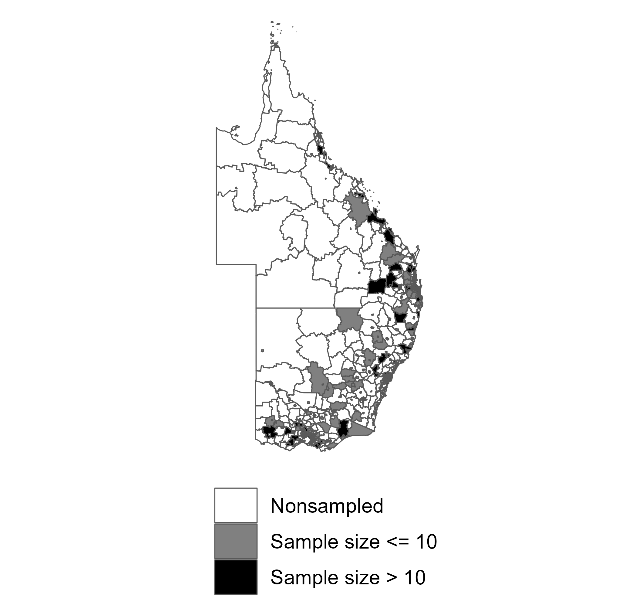
Figure 4: Map of the 1630 statistical area level 2 (SA2s) on the east coast of Australia. Each SA2 is colored according to the sample size (greater or less than 10) or sample status of the SA2 (sampled or nonsampled).

The individual level survey data were obtained from the 2017-18 National Health Survey (NHS), which is an Australia-wide population-level health survey conducted every 3-4 years by the Australian Bureau of Statistics (ABS) [69, 70]. The survey aimed to collect a variety of health data on one adult and one child (where possible) in each selected household. Households were selected using a complex multistage design [69]. Trained ABS interviewers conducted personal interviews with selected persons in each of the sampled households. To allow researchers to accommodate the complex sample design, the ABS provides survey weights, which we use in this analysis after applying the necessary rescalings (see Section 2.1). For the area level auxiliary data, we use data from the 2016 Australian census, represented as proportions. We obtained the Estimated Resident Population (ERP) stratified by age (15 years and above), sex and small area for both 2017 and 2018. In this study, the population counts were derived by averaging across the two years. Although the 2017-18 NHS collected data across Australia, we reduced our analysis to just those states on the east coast, both to ease the interpretation of visualizations and reduce the computation time.

We classify current smoking as daily, weekly, or less-than-weekly smokers, like the Social Health Atlas [1]. We additionally enforce that all current smokers must have smoked at least 100 cigarettes in their lifetime. After exclusions, we have data for 10,918 respondents aged 15 years and above. The overall weighted prevalence of current smoking in our study region is 14.7%.

The goal of this analysis is to generate prevalence estimates for 1,630 small areas, of which 1,262 (77%) were sampled. Of the sampled areas, 781 (62%) gave stable direct estimates. Area level sample sizes range from 1 to 140, with a median of 7.

The small areas we use are derived from the 2016 Australia Statistical Geography Standard (ASGS), which is the geographic standard maintained by the ABS [71]. The ASGS splits Australia into a hierarchical structure of areas that completely cover the country. We generate prevalence estimates at the statistical areas level 2 (SA2), which is the lowest level of the ASGS hierarchy for which detailed census population characteristics are publicly available.

5.2 Model details

Variable selection is an intricate step of our approach in practice. Not only do we have two models for which variable selection must be performed, but variable selection decisions made at the second stage are dependent on the model fit at the first stage; an issue we do not tackle in the current paper.

Given the extensive range of covariates available in the 2017-18 NHS, we used two phases of variable selection to mitigate the computational burden. First, as recommended by Goldstein [72], we employed frequentist inference methods (i.e. the lme4 package [73]) to identify an initial set of candidate fixed effects. Models were evaluated based on the AIC, BIC, and ALC, with a preference for lower AIC and BIC values. This frequentist stage served as an effective initial filter for variable selection.

Second, final decisions on covariates and random effects were made using Bayesian leave-one-out cross-validation (LOOCV) [74], which provided a Bayesian assessment of model fit with higher values preferred. The use of the loo package necessitated an approximation that disregarded the uncertainty from the stage 1 model.

Where possible the fixed and random effects for all the models were chosen according to the TSLN approach. That is, to enable fair comparisons, fixed and random effects for all models were as similar as possible. See Supplemental Materials B [49] for further details of model selection.

5.2.1 Individual level models

We used the following individual level categorical covariates in the TSLN-S1 model: age, sex and their interaction; registered marital status; high school completion status; Kessler psychological distress score; educational qualifications; self-assessed health; and labor force status. We also used the following household level categorical covariates: number of daily smokers, tenure type, and whether there were Indigenous Australian household members. Along with the individual and household level covariates, we used some SA2-level contextual covariates including state, the Index of Relative Socio-Economic Disadvantage (IRSD) from the Socio-Economic Indexes for Areas (SEIFA) [75], and the following SA2-level demographic variables as proportions: occupation, Indigenous Australian status, income, unemployment and household composition.

In addition to the individual and area level fixed effects, we introduced a random effect on a new categorical covariate, constructed from every unique combination of sex, age, and four binary-coded individual level risk factors (see Table 4 in the Supplemental Materials). The resulting covariate had 274 groups, with the number of participants in each category ranging from 1 to 299, with a median of 20.

To further improve the predictive accuracy of the TSLN-S1 model and increase the ALC, the final component of the model was an individual level residual error term with a fixed standard deviation of 0.5. The chosen TSLN-S1 model had $\text{ALC}=0.67$.

Since census microdata was unavailable, we could not mirror the TSLN-S1 model complexity in the LOG model. We omitted the risk factor categorical random effect and were restricted to just three individual level covariates: age, sex and marital status. These three covariates gave a poststrata dataset with 146,700 rows. Note that we also omitted the individual level residual error term from the LOG model as, unlike the TSLN-S1 model, the LOG model must prioritize generalisability in order to perform well.

Further details and definitions for the covariates used in the individual level models can be found in Supplemental Materials B [49].

5.2.2 Area level models

For both the TSLN-S2 and ELN models, we utilized the following SA2-level covariates: IRSD, state and the first six principal components derived from SA2-level census proportion data. Similar to Section 2.2.5 we use GVFs where the log of the SA2-level sample sizes was the only predictor. Details on variable selection and the covariates used in the area level models can be found in Supplemental Materials D [49].

5.2.3 Spatial random effects

Unlike in the simulation study where data were not generated with any spatial autocorrelation, we expect smoking prevalence to exhibit spatial clustering as smoking is generally higher in areas of lower socioeconomic status which can be geographical neighbors [76]. There is a considerable collection of research that develops spatial SAE models [77, 78, 79, 80]. Further, it has been shown that accommodating spatial structure in model-based SAE methods can provide considerable efficiency gains [42, 33, 81, 29, 14].

To adjust for the spatial autocorrelation between areas and enforce global and local smoothing, we use the BYM2 prior [43] at the SA2-level for the TSLN-S2, ELN and LOG models (see Supplemental Materials D [49] for details). Although others have used conditional autoregressive (CAR) or simultaneous autoregressive (SAR) priors only, Gomez-Rubio et al. [68] conclude that models with just the CAR prior generally over-estimate the small area estimates and argue that including a structured and unstructured random effect provides a useful compromise between producing accurate small area estimates and their corresponding variances.

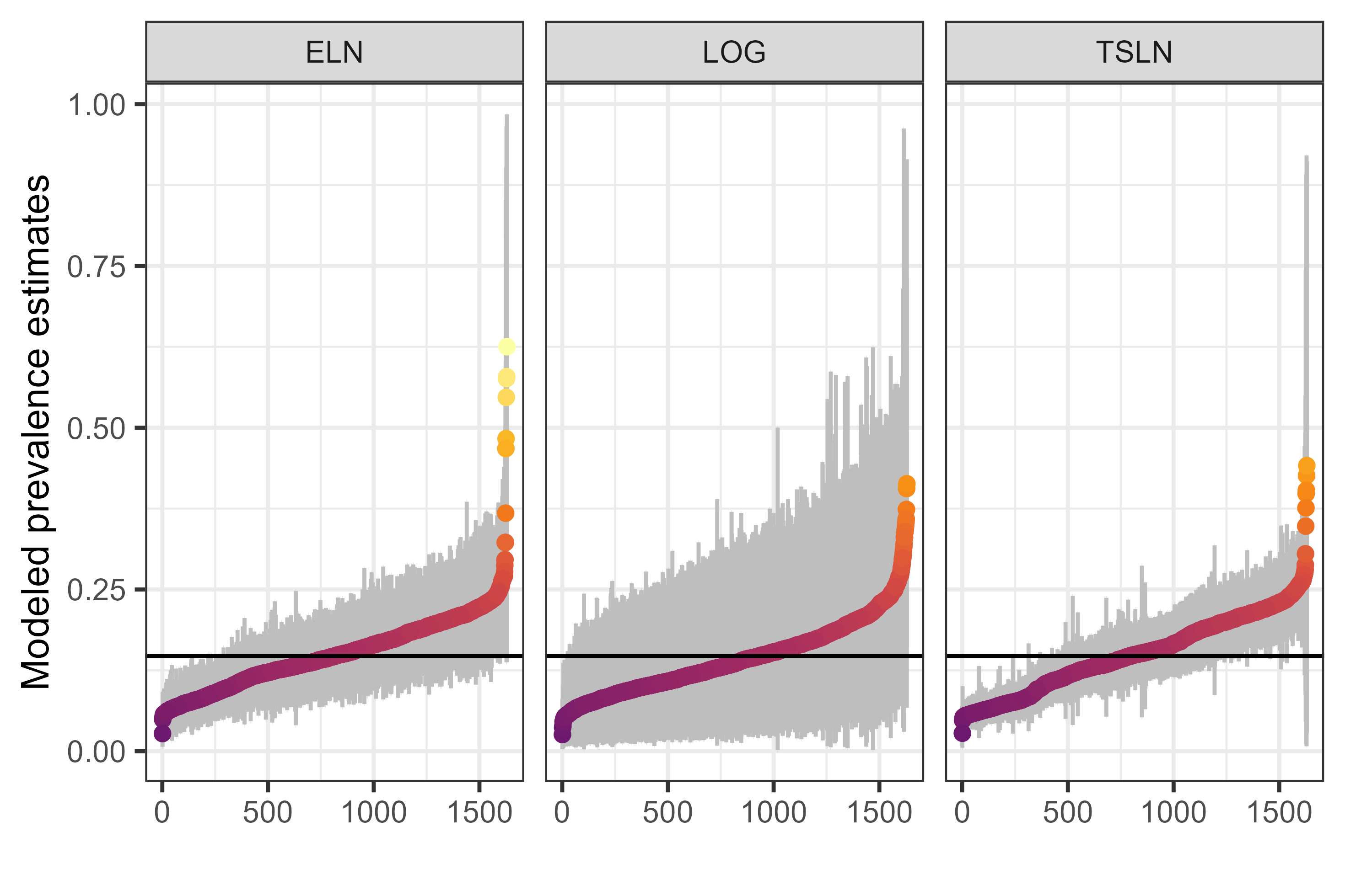
Figure 5: Comparison of the modeled SA2 level current smoking prevalence estimates from the three models. The caterpillar plots display the posterior medians and 95% highest density intervals (grey bars) for all 1630 SA2s, ordered by their magnitude. The point colors mirror the $y$-axis and the vertical black line is the overall current smoking prevalence.

5.2.4 Priors and computation

Most of the priors used in this case study mirror those specified in Section 4. We utilized a relatively informative prior for $\rho$, the mixing parameter of the BYM2 spatial prior which controls the amount of spatially structured as opposed to unstructured variation, where $\rho=1$ gives a scaled intrinsic CAR prior [43]. We use $\rho\sim$Beta$\left(\text{shape}=3.05,\text{rate}=1.65\right)$, a prior which places roughly 45% of density above $\rho=0.7$. In this application, areas with survey data may have many neighbors but few with survey data, thus this informative prior “encouraged” the models to borrow information locally. The median number of neighbors is 7, whereas the median number that has sampled data is 5. This informative prior on $\rho$ slightly improved both model fit and predictive accuracy. The posterior median of $\rho$ was 0.89 under this informative prior, but 0.5 under a Uniform$(0,1)$ prior.

We used $5000$ post-warmup draws for each of four chains in Stan [64], feeding a random subset of 500 posterior draws from the TSLN-S1 to the TSLN-S2 model. For storage reasons we thinned the draws by four, resulting in $5000$ useable posterior draws. Convergence of the models was assessed using $\widehat{R}$ [66], where a $\widehat{R}<1.02$ was used as the cutoff for convergence for the parameters of interest, namely $\boldsymbol{\mu}$. We also explored trace plots and autocorrelation plots to verify convergence. All proportion parameters, $\boldsymbol{\mu}$, had effective sample sizes $>$500.

5.2.5 Benchmarking

To help validate our small area estimates, we utilized state-level estimates as internal benchmarks [44]. There are four states on the east coast of Australia, with a median sample and population size of 3100 and 4.6 million, respectively. At this level of aggregation, the direct estimates are reliable. We employed inexact fully Bayesian benchmarking [46], which acts as a soft constraint on the model by penalizing discrepancies between the modeled state estimates and the direct state estimates. Unlike previous approaches that use posterior point estimates [39], Bayesian benchmarking directly includes the benchmarks in the joint posterior distribution, which accounts for benchmarking-induced uncertainty. We use Bayesian benchmarking in the TSLN-S2 and ELN models and exact benchmarking for the LOG model. Full details and a performance comparison with and without benchmarking is given in Supplemental Materials D [49].

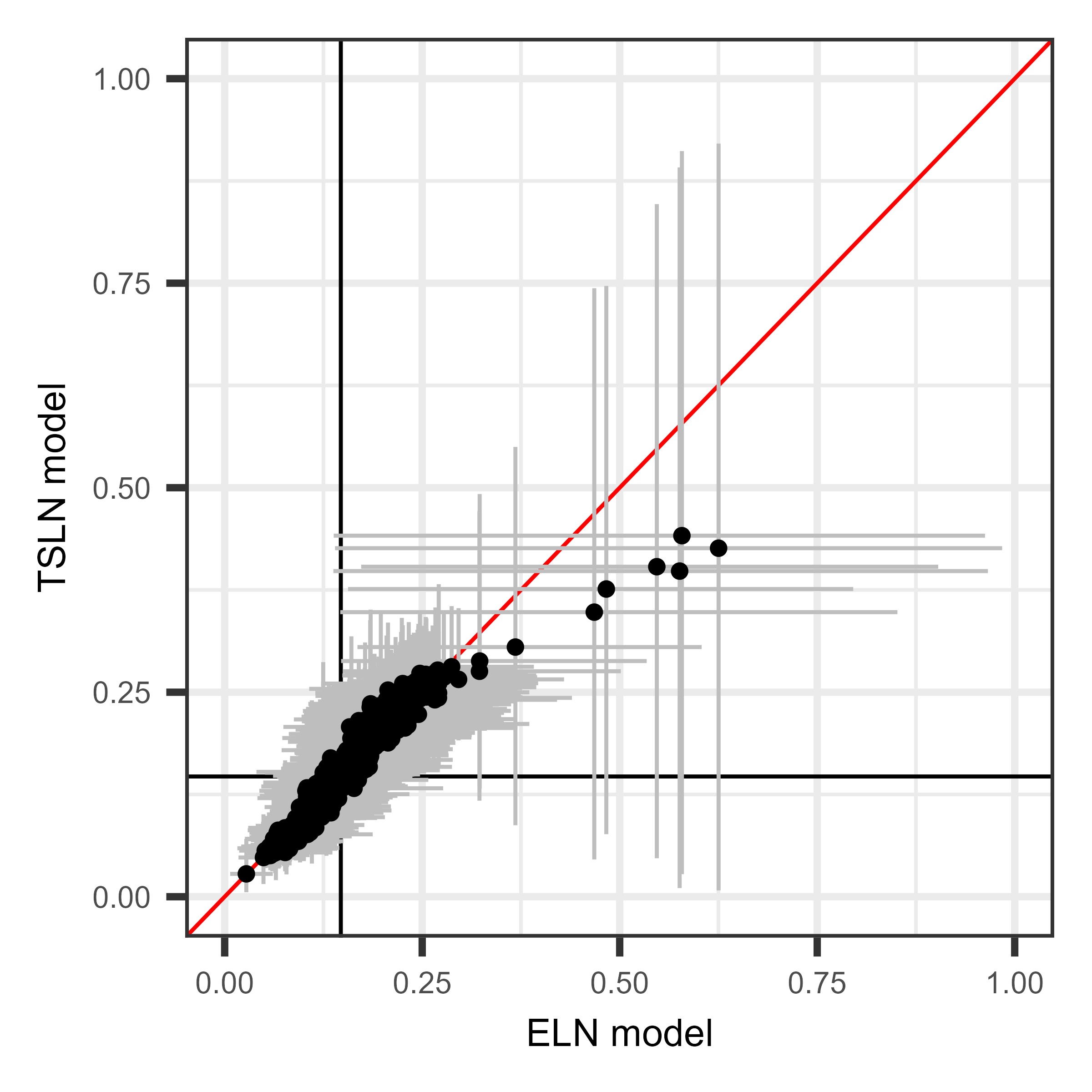
(a)

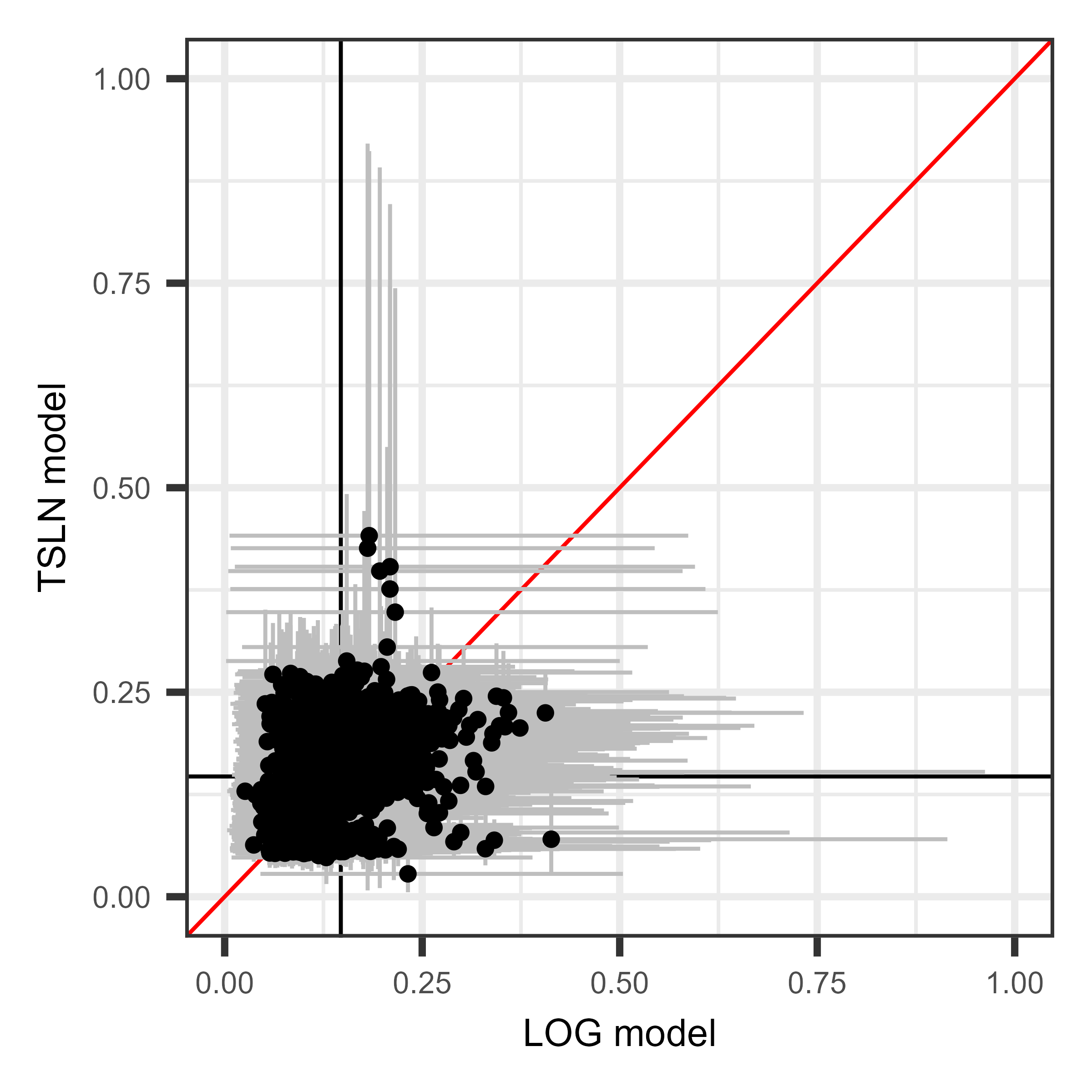
(b)

(c)

Figure 6: Comparison of the modeled estimates from the TSLN, LOG and ELN models. The scatter plots display the posterior medians (black points) and 95% highest density intervals (gray bars) of the modeled SA2 level current smoking prevalence estimates, with the red lines denoting equivalence. The vertical and horizontal black lines are the overall current smoking prevalence.

5.2.6 Visualisations

We map both absolute and relative measures of current smoking. The absolute measures are the posterior medians and highest density intervals (HDIs) of the estimated prevalence from the models, while the relative measures rely on odds ratios (ORs). We derive ORs as follows,

$$\widehat{\text{OR}}_{i}=\frac{\hat{\mu}_{i}/(1-\hat{\mu}_{i})}{\hat{\mu}^{D}/(1-\hat{\mu}^{D})},$$ (15)

where $\hat{\mu}^{D}$ is the overall direct estimate of current smoking prevalence. By deriving $\widehat{\text{OR}}_{i}$ for all posterior draws, we can map their posterior medians and HDIs. To quantify whether an OR is significantly different to 1, we use the exceedance probability (EP) [82, 59], where $t=1,\dots,T$ indexes the MCMC draws.

$$EP_{i}=\left(\frac{1}{T}\sum_{t}\mathbb{I}\left(\widehat{\text{OR}}_{it}>1\right)\right)$$ (16)

A high (low) $EP_{i}$ is interpreted as a high level of evidence that the OR for SA2 $i$ is significantly higher (lower) than 1. Generally an $EP_{i}$ above 0.8 or below 0.2 is considered significant [83].

5.3 Results

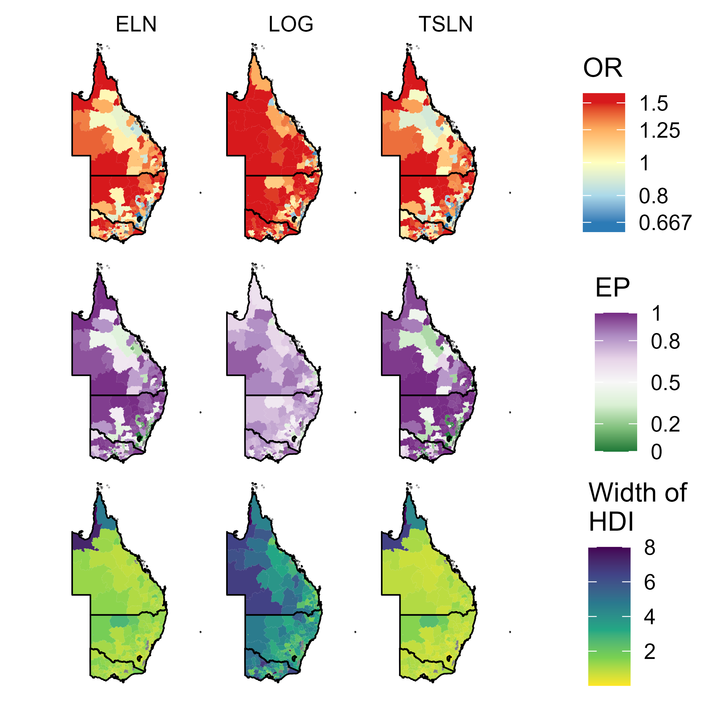
Figure 7: Choropleth maps displaying the modeled ORs for smoking prevalence in 1630 SA2s on the east coast of Australia. For each model, this figure displays the posterior medians (top row), exceedance probabilities ($EP$s) (middle row) and width of the 95% HDI (bottom row) for the ORs. Note that some values are lower than the range of color scales shown — for these values, the lowest color is shown. Gray areas were excluded from estimation due to having 2016-2017 ERPs smaller than or equal to 10. Black lines represent the boundaries of the four states on the east coast of Australia.

Fig. 5 gives separate caterpillar plots for the SA2-level prevalence estimates and HDIs for the three models. Supporting this plot, Fig. 6 compares the estimates from the TSLN approach to the ELN and LOG models. Both figures show the similarities in the modeled estimates from the two area level models and the superior interval sizes of the TSLN approach. The LOG model provides estimates with little correspondence to those from the TSLN or the ELN models.

For areas with high prevalence the TSLN approach provides more conservative estimates than those from the ELN model; a result of the two stages of smoothing applied when using the TSLN approach. Given that the sparsity of the survey data results in very noisy and unstable direct estimates, in this case study we prefer estimates that are slightly over-smoothed rather than undersmoothed.

The six outlying points visible in (a) of Fig. 6 are SA2s in the Cape York (Northern section) region of Queensland. The high level of uncertainty for these SA2s is reasonable as they are remote, have small populations and are far from areas with survey data.

In Fig. 7 we map the relative measures for all 1630 SA2s, including those without survey data. The figure displays posterior median ORs, HDIs and corresponding $EP$s for the three models. Observe that because the area level models (TSLN and ELN) generally provide more certainty in the estimates, the $EP$s are more extreme than those for the LOG model. The prevalence of current smoking is significantly higher than the overall prevalence in the western and northern parts of the region, while significantly lower in urban centers, such as Sydney (the most populous city on the east coast of Australia), Melbourne and Brisbane. Fig. 8 gives the absolute prevalence estimates for these three cities. See Supplemental Materials D [49] for a plot stratifying the modeled estimates by socioeconomic status and maps of the absolute prevalence estimates from the models.

By treating the direct estimates at a higher aggregation level as the truth, we compare the direct and modeled estimates at the statistical area level 4 using RRMSE, ARB, coverage and interval overlap. The details and possible limitations of these comparative performance results are given in Supplemental Materials D [49]. We found that the TSLN approach provided superior MRRMSE and interval overlap. Furthermore, the performance metrics for the TSLN approach show the smallest changes when we benchmark, providing more support for the validity of the estimates from the TSLN approach. Prevalence estimates from the LOG model, on the other hand, saw considerable changes when benchmarking was applied. We posit that the LOG model is providing poor estimates given the restricted set of individual level census covariates that were available, given the requirements of the LOG model.

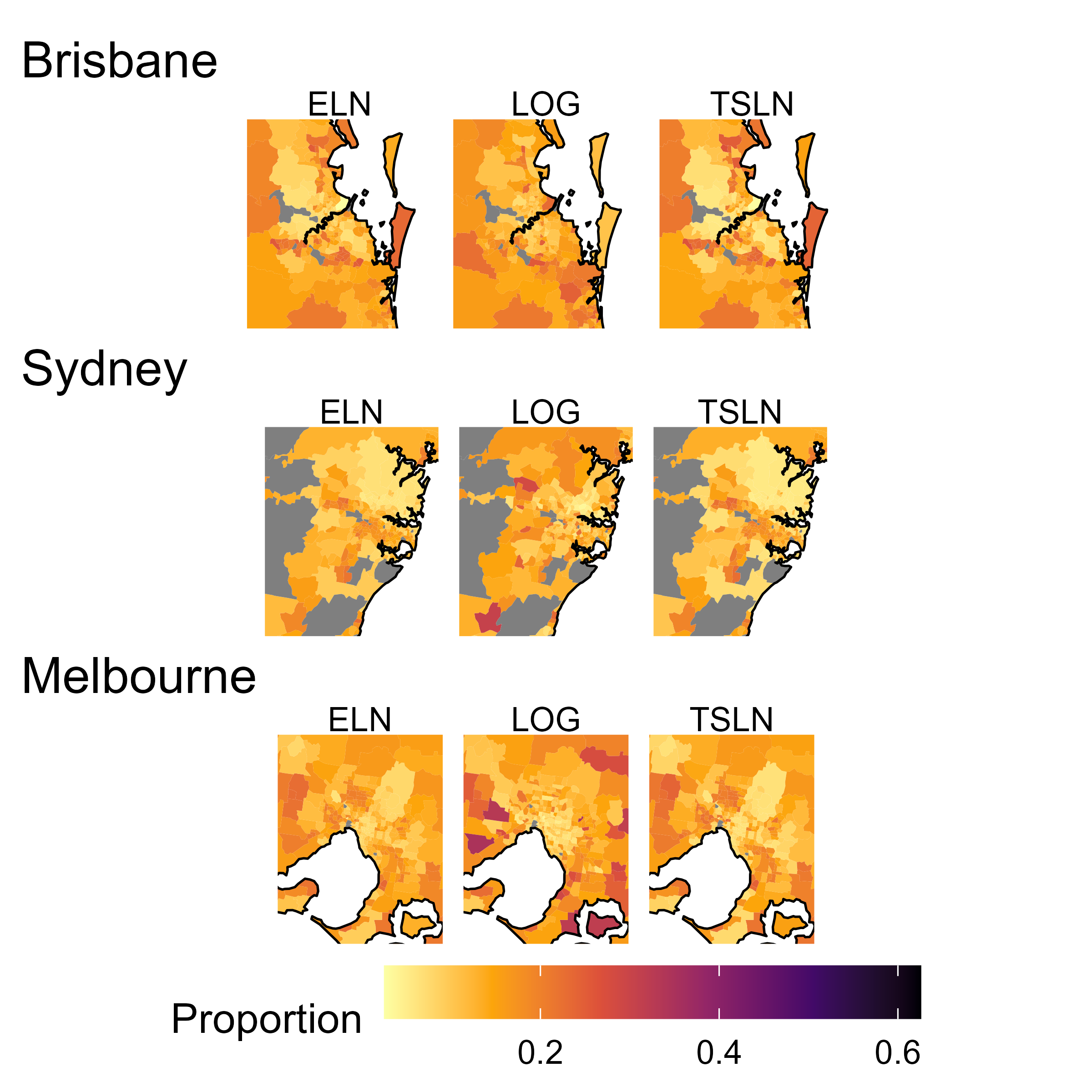
Figure 8: Choropleth inset maps displaying the modeled estimates of the proportion of current smokers in and around Sydney, Melbourne and Brisbane; three capital cities on the east coast of Australia. Gray areas were excluded from estimation due to having 2016-2017 ERPs smaller than or equal to 10. Most of these excluded areas are National parks, industrial areas, airports or cemeteries.

6 Discussion

We have proposed a new Bayesian model-based SAE approach to estimate proportions for small areas from sparse survey data. The TSLN approach is able to model these data by using both individual and area level models to reduce instability, alleviate covariate restrictions, and generate estimates for nonsampled areas. We have shown that the TSLN approach can provide superior proportion estimates for sampled and nonsampled areas compared to some alternatives, with similar or slightly more bias but much smaller variance; resulting in consistently smaller MRRMSEs and credible intervals. Compared with other available approaches, the TSLN approach appears to be the best option in sparse settings, such as when using the NHS in Australia. Moreover, we have demonstrated, along with others [29, 30], that the multi-stage or double smoothing properties of modeling at both the individual and area level are beneficial across a broad range of SAE applications.

Although the simulation results and case study illustrate the potential benefits of the TSLN approach, some limitations motivate future theoretical and applied research in two-stage SAE. One pressing need is the development of statistical theory to motivate the use of double smoothing and two-stage approaches in general.

Our approach follows the independence assumptions proposed by Gao and Wakefield [29], but the potential for correlation among the S1 estimates warrants further investigation. Das et al. [30] found that incorporating the covariances between area predictions did little to improve the bias or variance of their final estimates. Our own simulation study corroborated the low correlation between S1 estimates. We provide further details in Supplemental Material A. Future research could assess the validity and implications of this independence assumption. One option is to create a specialized MCMC algorithm, which would eliminate the need for these assumptions and allow one to fit the TSLN approach in a single step. Alternatively, our TSLN approach could be conceptualized as a modular model, by leveraging Bayesian cut distributions [84].

We recognize that the GVF applied exclusively to unstable S1 sampling variances represents a unique solution to the undesirable properties mentioned in Section 2.2.5. Thus, another area of exploration is the development of non-GVF solutions. Alternatively, methods to adjust for the instability of direct estimates could be formally compared. On a related note, while coverage was relatively stable for the TSLN approach, one could explore methods of conformal prediction [85], which can be used to guarantee frequentist coverage in small area estimation [86].

The Gaussian distribution assumption in the stage 2 model, although consistent with existing literature [29], presents another limitation. The empirical logistic transformation of direct estimates yields a small set of possible values if area level sample sizes are small. This issue is alleviated when using our S1 estimates, which aggregate probabilities rather than binary variables. Although the smoothing introduced by the stage 1 model makes the Gaussian assumption more plausible, especially under data sparsity, further theoretical work is required to determine when the assumption becomes inappropriate. We initially explored an alternative approach using a Beta likelihood, but encountered issues with MCMC convergence and unidentifiability, warranting future research.

Another consideration is substantial clustering of the sampling, which results in the effective sample size of the survey being significantly lower than the nominal sample size. While the current study does not delve into the specific impacts of clustering, the stage 1 model is inherently flexible and is therefore capable of accommodating clustering effects similar to standard individual-level logistic models.

The TSLN approach is generic in its component models, which within an applied context allows researchers to extend our approach by using more flexible classes of models (such as semi or non-parametric models or even machine learning algorithms), as long as uncertainty can be captured. Performance could be improved by leveraging robust SAE for the component models, such as those developed by Chambers et al. [87] or Liu and Lahiri [23].

Alternatively, the TSLN approach could be extended to the multivariate setting by using univariate stage 1 models, followed by a multivariate stage 2 model [80, 88]. Finally, further work is required to develop model selection tools for both stages of the TSLN approach, with a focus on the flow-on effect of model choices from the first stage to the second and how LOOCV can be better utilized in this setting.

7 Conclusion

Given that the need for higher resolution area level estimates is increasing faster than funding for larger surveys, methods of SAE must be capable of tackling sparsity issues. In this work, we have developed a solution to SAE for severely sparse data by leveraging both area and individual level models. Similar to other work [29, 30], this research represents another important step in continuing the positive narrative surrounding two-stage approaches and highlights their benefits and future avenues of research in SAE. As expressed by Fuglstad et al. [10], “$\dots$ the goal of the analysis should determine the approach, and different goals may call for different approaches.” We envisage that our approach will allow practitioners to set more ambitious goals for their small area estimates in the future.

Acknowledgments

This study has received ethical approval from the Queensland University of Technology Human Research Ethics Committee (Project ID: 4609) for the project entitled “Statistical methods for small area estimation of cancer risk factors and their associations with cancer incidence”.

We thank the Australian Bureau of Statistics (ABS) for designing and collecting the National Health Survey data and making it available for analysis in the DataLab. The views expressed in this paper are those of the authors and do not necessarily reflect the policy of QUT, CCQ or the ABS.

Competing interests

The authors declare that they have no competing interests.

Funding

JH was supported by the Queensland University of Technology (QUT) Centre for Data Science and Cancer Council QLD (CCQ) Scholarship. SC receives salary and research support from a National Health and Medical Research Council Investigator Grant (#2008313).

Supplemental materials

The supplemental material mentioned throughout this work can be found on at the end of this document. This additional material includes further details, plots and results to accompany Sections 2-5 of this paper.

References

- PHIDU [2018] PHIDU. Social health atlases, 2018. https://phidu.torrens.edu.au/social-health-atlases.
- Duncan et al. [2019a] E. W. Duncan, S. M. Cramb, J. F. Aitken, K. L. Mengersen, and P. D. Baade. Development of the Australian Cancer Atlas: Spatial modelling, visualisation, and reporting of estimates. International Journal of Health Geographics, 18(1):1–12, 2019a. doi:10.1186/s12942-019-0185-9. URL https://www.scopus.com/inward/record.uri?eid=2-s2.0-85072763102&doi=10.1186%2fs12942-019-0185-9&partnerID=40&md5=9b36caf529353c1c2096d322009360ff.
- Rao and Molina [2015] J.N.K. Rao and Isabel Molina. Small Area Estimation. Wiley Series in Survey Methodology, Hoboken, New Jersey, 2nd edition, 2015.
- Pratesi [2016] M. Pratesi. Analysis of Poverty Data by Small Area Estimation. Wiley Series in Survey Methodology. Wiley, 2016.
- Morales et al. [2021] D. Morales, M.D. Esteban, A. Pérez, and T. Hobza. A Course on Small Area Estimation and Mixed Models. Springer, 2021.
- Horvitz and Thompson [1952] D. Horvitz and D. Thompson. A generalisation of sampling without replacement from a finite universe. Journal of the American Statistical Association, 47:663–685, 1952.
- Battese et al. [1988] George E. Battese, Rachel M. Harter, and Wayne A. Fuller. An error-components model for prediction of county crop areas using survey and satellite data. Journal of the American Statistical Association, 83(401):28–36, 1988. ISSN 0162-1459. doi:10.108001621459.1988.10478561.
- Fay and Herriot [1979] Robert E. Fay and Roger A. Herriot. Estimates of income for small places: An application of james-stein procedures to census data. Journal of the American Statistical Association, 74(366):269–277, 1979. ISSN 01621459. doi:10.2307/2286322.
- Moretti and Whitworth [2021] A. Moretti and A. Whitworth. Estimating the uncertainty of a small area estimator based on a microsimulation approach. Sociological Methods and Research, 2021. doi:10.1177/0049124120986199.
- Fuglstad et al. [2021] Geir-Arne Fuglstad, Zehang Richard Li, and Jon Wakefield. The two cultures for prevalence mapping: Small area estimation and spatial statistics. arXiv preprint arXiv:2110.09576, 2021. doi:arXiv:2110.09576.
- Liu et al. [2007] Benmei Liu, Partha Lahiri, and Graham Kalton. Hierarchical bayes modeling of survey-weighted small area proportions. Proceedings of the American Statistical Association, Survey Research Section, pages 3181–3186, 2007.
- Janicki [2020] R. Janicki. Properties of the beta regression model for small area estimation of proportions and application to estimation of poverty rates. Communications in Statistics - Theory and Methods, 49(9):2264–2284, 2020. doi:10.1080/03610926.2019.1570266.
- Liu et al. [2014] B. Liu, P. Lahiri, and G. Kalton. Hierarchical bayes modeling for survey-weighted small area proportions. Survey Methodology, 40(1):1–13, 2014.
- Paige et al. [2022] John Paige, Geir-Arne Fuglstad, Andrea Riebler, and Jon Wakefield. Design-and model-based approaches to small-area estimation in a low-and middle-income country context: comparisons and recommendations. Journal of Survey Statistics and Methodology, 10(1):50–80, 2022. ISSN 2325-0984.
- Wolter [2007] Kirk M. Wolter. Introduction to Variance Estimation. Springer, New York, NY, 2007. doi:https://doi.org/10.1007/978-0-387-35099-8.
- Ospina and Ferrari [2012] Raydonal Ospina and Silvia L. P. Ferrari. A general class of zero-or-one inflated beta regression models. Computational Statistics and Data Analysis, 56(6):1609–1623, 2012. ISSN 0167-9473. doi:https://doi.org/10.1016/j.csda.2011.10.005. URL https://www.sciencedirect.com/science/article/pii/S0167947311003628.
- De Nicolò and Gardini [2022] Silvia De Nicolò and Aldo Gardini. The r package tipsae: Tools for mapping proportions and indicators on the unit interval. Report, 2022.
- Mercer et al. [2014] Laina Mercer, Jon Wakefield, Cici Chen, and Thomas Lumley. A comparison of spatial smoothing methods for small area estimation with sampling weights. Spatial Statistics, 8(1):69–85, 2014. ISSN 2211-6753. doi:https://doi.org/10.1016/j.spasta.2013.12.001.
- Chen et al. [2014] Cici Chen, Jon Wakefield, and Thomas Lumely. The use of sampling weights in bayesian hierarchical models for small area estimation. Spatial and Spatio-temporal Epidemiology, 11:33–43, 2014. ISSN 1877-5845. doi:https://doi.org/10.1016/j.sste.2014.07.002. URL https://www.sciencedirect.com/science/article/pii/S1877584514000367.
- Malec et al. [1997] Donald Malec, J. Sedransk, Christopher L. Moriarity, and Felicia B. Leclere. Small area inference for binary variables in the national health interview survey. Journal of the American Statistical Association, 92(439):815–826, 1997. ISSN 0162-1459. doi:10.1080/01621459.1997.10474037. URL https://doi.org/10.1080/01621459.1997.10474037.
- Moura and Migon [2002] F. A. S. Moura and H. S. Migon. Bayesian spatial models for small area estimation of proportions. Statistical Modeling, 2(3):183–201, 2002. doi:10.1191/1471082x02st032oa.
- Chen and Lahiri [2012] S. Chen and P. Lahiri. Inferences on small area proportions. Journal of the Indian Society of Agricultural Statistics, 66(1):121–124, 2012.
- Liu and Lahiri [2017] Benmei Liu and Partha Lahiri. Adaptive hierarchical bayes estimation of small area proportions. Calcutta Statistical Association Bulletin, 69(2):150–164, 2017.
- Gelman [2007] Andrew Gelman. Struggles with survey weighting and regression modeling. Statistical Science, 22(2):153–164, 2007. URL https://doi.org/10.1214/088342306000000691.
- Gelman and Little [1997] Andrew Gelman and Thomas C Little. Poststratification into many categories using hierarchical logistic regression. Survey Methodology, pages 23:127–135, 1997.
- Leemann and Wasserfallen [2017] Lucas Leemann and Fabio Wasserfallen. Extending the use and prediction precision of subnational public opinion estimation. American Journal of Political Science, 61(4):1003–1022, 2017. ISSN 0092-5853. doi:https://doi.org/10.1111/ajps.12319.
- Kuriwaki and Yamauchi [2021] Shiro Kuriwaki and Soichiro Yamauchi. Synthetic area weighting for measuring public opinion in small areas. arXiv preprint arXiv:2105.05829, 2021. doi:arXiv:2105.05829.
- Honaker and Plutzer [2011] James Honaker and Eric Plutzer. Small area estimation with multiple overimputation. Midwest Political Science Association, Chicago, 2011.
- Gao and Wakefield [2023] Peter A. Gao and Jon Wakefield. Smoothed model-assisted small area estimation of proportions. Canadian Journal of Statistics, 2023. doi:https://doi.org/10.1002/cjs.11787.
- Das et al. [2022] S. Das, J. van den Brakel, H.J. Boonstra, and S. Haslett. Multilevel time series modelling of antenatal care coverage in bangladesh at disaggregated administrative levels. Survey Methodology, 48(2), 2022. URL http://www.statcan.gc.ca/pub/12-001-x/2022002/article/00010-eng.htm.
- Baffour et al. [2019] B. Baffour, H. Chandra, and A. Martinez. Localised estimates of dynamics of multi-dimensional disadvantage: An application of the small area estimation technique using australian survey and census data. International Statistical Review, 87(1):1–23, 2019.
- ABS [2019] ABS. Modelled estimates for small areas based on the 2017-18 National Health Survey. Report, Australian Bureau of Statistics, 2019.
- Vandendijck et al. [2016] Y. Vandendijck, C. Faes, R. S. Kirby, A. Lawson, and N. Hens. Model-based inference for small area estimation with sampling weights. Spatial Statistics, 18(1):455–473, 2016. doi:10.1016/j.spasta.2016.09.004.
- Parker et al. [2019] Paul A. Parker, Ryan Janicki, and Scott H. Holan. Unit level modeling of survey data for small area estimation under informative sampling: A comprehensive overview with extensions. arXiv preprint arXiv:1908.10488, 2019. doi:arXiv:1908.10488.
- Cislaghi et al. [1990] C. Cislaghi, M. Braga, A. Danielli, and G. Luppi. An analysis of the spatial association between cancer mortality and risk factor: the role of the geographical scale. Espace-Populations-Societes, 8(3):407–416, 1990. doi:10.3406/espos.1990.1418. URL https://www.scopus.com/inward/record.uri?eid=2-s2.0-0025631992&doi=10.3406%2fespos.1990.1418&partnerID=40&md5=1bf6104faa0099b62fa1ecdf7210bed5https://www.persee.fr/doc/espos_0755-7809_1990_num_8_3_1418.
- Rao [2011] J. N. K. Rao. Impact of frequentist and bayesian methods on survey sampling practice: A selective appraisal. Statistical Science, 26(2):240–256, 2011. doi:10.1214/10-STS346. URL https://doi.org/10.1214/10-STS346.
- Hajek [1971] J. Hajek. Comment on "an essay on the logical foundations of survey sampling, part one". The Foundations of Survey Sampling, 1971.
- Cassy et al. [2022] S. R. Cassy, S. Manda, F. Marques, and Mdro Martins. Accounting for sampling weights in the analysis of spatial distributions of disease using health survey data, with an application to mapping child health in malawi and mozambique. International Journal of Environmental Research and Public Health, 19(10), 2022. ISSN 1661-7827 (Print) 1660-4601. doi:10.3390/ijerph19106319.
- Pfeffermann [2013] Danny Pfeffermann. New important developments in small area estimation. Statistical Science, 28(1):40–68, 2013.
- Iriondo-Perez et al. [2018] Jeniffer Iriondo-Perez, Amang Sukasih, and Rachel Harter. Comparing direct survey and small area estimates of health care coverage in new york. Report, American Statistical Association, 2018.
- Roy et al. [2019] Paritosh K. Roy, Md Hasinur R. Khan, Tahmina Akter, and M. Shafiqur Rahman. Exploring socio-demographic-and geographical-variations in prevalence of diabetes and hypertension in bangladesh: Bayesian spatial analysis of national health survey data. Spatial and Spatio-temporal Epidemiology, 29:71–83, 2019. ISSN 1877-5845. doi:https://doi.org/10.1016/j.sste.2019.03.003.
- Chung and Datta [2020] Hee Cheol Chung and Gauri Sankar Datta. Bayesian hierarchical spatial models for small area estimation. Report, Center for Statistical Research and Methodology, 2020.
- Riebler et al. [2016] Andrea Riebler, Sigrunn H. Sørbye, Daniel Simpson, and Håvard Rue. An intuitive bayesian spatial model for disease mapping that accounts for scaling. arXiv preprint arXiv:1601.01180, 2016. doi:arXiv:1601.01180.
- Bell et al. [2013] W. R. Bell, G. S. Datta, and M. Ghosh. Benchmarking small area estimators. Biometrika, 100(1):189–202, 2013. ISSN 0006-3444. doi:10.1093/biomet/ass063. URL <GotoISI>://WOS:000315623900011.
- Datta et al. [2011] G. Datta, M. Ghosh, R. Steorts, and J. Maples. Bayesian benchmarking with applications to small area estimation. TEST, 20:574–588, 2011.
- Zhang and Bryant [2020] J. L. Zhang and J. Bryant. Fully bayesian benchmarking of small area estimation models. Journal of Official Statistics, 36(1):197–223, 2020. ISSN 0282-423X. doi:10.2478/jos-2020-0010. URL <GotoISI>://WOS:000520863200010.
- Binder [1983] David A Binder. On the variances of asymptotically normal estimators from complex surveys. International Statistical Review, pages 279–292, 1983. ISSN 0306-7734.
- Savitsky and Toth [2016] Terrance D Savitsky and Daniell Toth. Bayesian estimation under informative sampling. Electronic Journal of Statistics, 10(1):1677–1708, 2016. ISSN 1935-7524.
- Hogg et al. [2023] James Hogg, Jessica Cameron, Susanna Cramb, Peter Baade, and Kerrie Mengersen. Supplement to "a two-stage bayesian method of small area estimation for proportions". International Statistical Review, 2023.
- Parker et al. [2023] Paul A Parker, Ryan Janicki, and Scott H Holan. A Comprehensive Overview of Unit-Level Modeling of Survey Data for Small Area Estimation Under Informative Sampling. Journal of Survey Statistics and Methodology, 11(4):829–857, 2023. doi:10.1093/jssam/smad020.
- You and Rao [2000] Yong You and JNK Rao. Hierarchical bayes estimation of small area means using multi-level models. Survey Methodology, 26(2):173–181, 2000.
- Gelman et al. [2020] Andrew Gelman, Aki Vehtari, Daniel Simpson, Charles C. Margossian, Bob Carpenter, Yuling Yao, Lauren Kennedy, Jonah Gabry, Paul-Christian Bürkner, and Martin Modrák. Bayesian workflow. arXiv preprint arXiv:2011.01808v1, 2020. doi:arXiv:2011.01808v1.
- Gao and Wakefield [2022] Peter A. Gao and Jon Wakefield. A spatial variance-smoothing area level model for small area estimation of demographic rates. arXiv preprint arXiv:2209.02602, 2022. doi:arXiv:2209.02602.
- Breidt and Jean [2017] F. Jay Breidt and D. Opsomer Jean. Model-assisted survey estimation with modern prediction techniques. Statistical Science, 32(2):190–205, 2017. doi:10.1214/16-STS589. URL https://doi.org/10.1214/16-STS589.
- Carroll et al. [2006] Raymond J. Carroll, David Ruppert, Leonard A. Stefanski, and Ciprian M. Crainiceanu. Measurement Error in Nonlinear Models : A Modern Perspective, Second Edition. CRC Press LLC, London, UNITED KINGDOM, 2006. ISBN 9781420010138. URL http://ebookcentral.proquest.com/lib/qut/detail.action?docID=274076.
- Tzavidis et al. [2018] N. Tzavidis, L. C. Zhang, A. Luna, T. Schmid, and N. Rojas-Perilla. From start to finish: a framework for the production of small area official statistics. Journal of the Royal Statistical Society, 181(4):927–979, 2018. ISSN 0964-1998. doi:10.1111/rssa.12364. URL <GotoISI>://WOS:000445193300002.
- Best et al. [2008] N. Best, S. Richardson, and P. Clarke. A comparison of model-based methods for small area estimation. Report, Department of Epidemiology and Public Health, Imperial College London, 2008.
- Hidiroglou and You [2016] M. Hidiroglou and Y. You. Comparison of unit level and area level small area estimators. Survey Methodology, 42(1):41–61, 2016.
- Dong and Wakefield [2021] Tracy Qi Dong and Jon Wakefield. Modeling and presentation of vaccination coverage estimates using data from household surveys. Vaccine, 39(18):2584–2594, 2021. ISSN 0264-410X.
- Aitkin et al. [2009] Murray Aitkin, Charles C. Liu, and Tom Chadwick. Bayesian model comparison and model averaging for small-area estimation. The Annals of Applied Statistics, 3(1):199–221, 2009. URL https://doi.org/10.1214/08-AOAS205.
- Buttice and Highton [2013] Matthew K. Buttice and Benjamin Highton. How does multilevel regression and poststratification perform with conventional national surveys? Political Analysis, 21(4):449–467, 2013. ISSN 10471987, 14764989.
- Guadarrama et al. [2021] María Guadarrama, Domingo Morales, and Isabel Molina. Time stable empirical best predictors under a unit-level model. Computational Statistics and Data Analysis, 160:107226, 2021. ISSN 0167-9473. doi:https://doi.org/10.1016/j.csda.2021.107226.
- Molina and Rao [2010] Isabel Molina and J. N. K. Rao. Small area estimation of poverty indicators. The Canadian Journal of Statistics, 38(3):369–385, 2010. ISSN 03195724. URL http://www.jstor.org/stable/27896031.
- Stan Development Team [2022a] Stan Development Team. Stan, 2022a. https://mc-stan.org.
- Plummer [2003] Martyn Plummer. Jags: A program for analysis of bayesian graphical models using gibbs sampling. In 3rd International Workshop on Distributed Statistical Computing, 2003.
- Vehtari et al. [2021] Aki Vehtari, Andrew Gelman, Daniel Simpson, Bob Carpenter, and Paul-Christian Bürkner. Rank-normalization, folding, and localization: An improved for assessing convergence of mcmc (with discussion). Bayesian Analysis, 16(2):667–718, 2021. doi:10.1214/20-BA1221. URL https://doi.org/10.1214/20-BA1221.
- Stan Development Team [2022b] Stan Development Team. The qr reparameterization. In Stan User’s Guide. 2022b. URL https://mc-stan.org/docs/stan-users-guide/QR-reparameterization.html.
- Gomez-Rubio et al. [2008] V. Gomez-Rubio, Nicky Best, Sylvia Richardson, Guangquan Li, and Philip Clarke. Bayesian statistics small area estimation. Report, Office for National Statistics, 2008.
- ABS [2018] ABS. National Health Survey: First results methodology. Report, Australian Bureau of Statistics, 2018. URL https://www.abs.gov.au/methodologies/national-health-survey-first-results-methodology/2017-18.
- ABS [2017] ABS. Microdata: National Health Survey [DataLab], 2017.
- ABS [2011] ABS. Australian Statistical Geography Standard (ASGS), 2011. URL https://www.abs.gov.au/websitedbs/d3310114.nsf/home/australian+statistical+geography+standard+(asgs).
- Goldstein [2011] Harvey Goldstein. Multilevel statistical models. John Wiley and Sons, 2011. ISBN 111995682X.
- Bates et al. [2015] Douglas Bates, Martin Mächler, Ben Bolker, and Steve Walker. Fitting linear mixed-effects models using lme4. Journal of Statistical Software, 67(1):1–48, 2015. doi:10.18637/jss.v067.i01.
- Vehtari et al. [2017] A. Vehtari, A. Gelman, and J. Gabry. Practical bayesian model evaluation using leave-one-out cross-validation and waic. Statistics and Computing, 27(5):1413–1432, 2017. doi:10.1007/s11222-016-9696-4. URL https://www.scopus.com/inward/record.uri?eid=2-s2.0-85026299835&doi=10.1007%2fs11222-016-9696-4&partnerID=40&md5=d4d48dc9b435386f7e4be2c5cb580f4b.
- ABS [2016] ABS. Technical paper: Socio-economic indexes for areas (SEIFA). Report, Australian Bureau of Statistics,, 2016.
- Patterson et al. [2014] K. A. E. Patterson, V. Cleland, A. Venn, L. Blizzard, and S. Gall. A cross-sectional study of geographic differences in health risk factors among young australian adults: The role of socioeconomic position. BMC Public Health, 14(1):1–10, 2014. doi:10.1186/1471-2458-14-1278. URL https://www.scopus.com/inward/record.uri?eid=2-s2.0-84924288776&doi=10.1186%2f1471-2458-14-1278&partnerID=40&md5=775e49b9ba2c4478ae77d0e0c641ce77.
- Saei and Chambers [2003] Ayoub Saei and Ray Chambers. Small area estimation under linear and generalized linear mixed models with time and area effects. Report, University of Southampton, 2003.
- Chandra and Salvati [2018] Hukum Chandra and Nicola Salvati. Small area estimation of proportions under a spatial dependent aggregated level random effects model. Communications in Statistics-Theory and Methods, 47(5):1234–1255, 2018.
- Chandra et al. [2017] Hukum Chandra, Nicola Salvati, and Ray Chambers. Small area prediction of counts under a non-stationary spatial model. Spatial Statistics, 20:30–56, 2017. ISSN 2211-6753. doi:https://doi.org/10.1016/j.spasta.2017.01.004.
- Guha and Chandra [2023] Saurav Guha and Hukum Chandra. Small area estimation under a spatially correlated multivariate area-level model. Journal of the Royal Statistical Society Series A: Statistics in Society, page qnad079, 06 2023. ISSN 0964-1998. doi:10.1093/jrsssa/qnad079.
- Donegan et al. [2021] Connor Donegan, Yongwan Chun, and Daniel A. Griffith. Modeling community health with areal data: Bayesian inference with survey standard errors and spatial structure. International Journal of Environmental Research and Public Health, 18(13):6856, 2021. ISSN 1660-4601. URL https://www.mdpi.com/1660-4601/18/13/6856.
- Duncan et al. [2019b] Earl W. Duncan, Susanna M. Cramb, Joanne F. Aitken, Kerrie L. Mengersen, and Peter D. Baade. Development of the australian cancer atlas: spatial modelling, visualisation, and reporting of estimates. International Journal of Health Geographics, 18(1):21, 2019b. ISSN 1476-072X. doi:10.1186/s12942-019-0185-9. URL https://doi.org/10.1186/s12942-019-0185-9.
- Richardson et al. [2004] Sylvia Richardson, Andrew Thomson, Nicky Best, and Paul Elliott. Interpreting posterior relative risk estimates in disease-mapping studies. Environmental Health Perspectives, 112(9):1016–1025, 2004. ISSN 0091-6765 1552-9924. doi:10.1289/ehp.6740.
- Jacob et al. [2017] Pierre E Jacob, Lawrence M Murray, Chris C Holmes, and Christian P Robert. Better together? statistical learning in models made of modules. arXiv preprint arXiv:1708.08719, 2017. doi:arXiv:1708.08719.
- Shafer and Vovk [2008] Glenn Shafer and Vladimir Vovk. A tutorial on conformal prediction. Journal of Machine Learning Research, 9(3), 2008. ISSN 1532-4435.
- Bersson and Hoff [2022] Elizabeth Bersson and Peter D Hoff. Optimal conformal prediction for small areas. arXiv preprint arXiv:2204.08122, 2022.
- Chambers et al. [2014] Ray Chambers, Hukum Chandra, Nicola Salvati, and Nikos Tzavidis. Outlier robust small area estimation. Journal of the Royal Statistical Society Series B: Statistical Methodology, 76(1):47–69, 2014.
- Arima et al. [2017] Serena Arima, William R Bell, Gauri S Datta, Carolina Franco, and Brunero Liseo. Multivariate fay–herriot bayesian estimation of small area means under functional measurement error. Journal of the Royal Statistical Society Series A: Statistics in Society, 180(4):1191–1209, 2017.