The Dyson Equalizer: Adaptive Noise Stabilization for Low-Rank Signal Detection and Recovery

Abstract

Detecting and recovering a low-rank signal in a noisy data matrix is a fundamental task in data analysis. Typically, this task is addressed by inspecting and manipulating the spectrum of the observed data, e.g., thresholding the singular values of the data matrix at a certain critical level. This approach is well-established in the case of homoskedastic noise, where the noise variance is identical across the entries. However, in numerous applications, the noise can be heteroskedastic, where the noise characteristics may vary considerably across the rows and columns of the data. In this scenario, the spectral behavior of the noise can differ significantly from the homoskedastic case, posing various challenges for signal detection and recovery. To address these challenges, we develop an adaptive normalization procedure that equalizes the average noise variance across the rows and columns of a given data matrix. Our proposed procedure is data-driven and fully automatic, supporting a broad range of noise distributions, variance patterns, and signal structures. We establish that in many cases, this procedure enforces the standard spectral behavior of homoskedastic noise – the Marchenko-Pastur (MP) law, allowing for simple and reliable detection of signal components. Furthermore, we demonstrate that our approach can substantially improve signal recovery in heteroskedastic settings by manipulating the spectrum after normalization. Lastly, we apply our method to single-cell RNA sequencing and spatial transcriptomics data, showcasing accurate fits to the MP law after normalization. Our approach relies on recent results in random matrix theory, which describe the resolvent of the noise via the so-called Dyson equation. By leveraging this relation, we can accurately infer the noise level in each row and each column directly from the resolvent of the data.

Keywords— principal components analysis, matrix denoising, rank estimation, noise stabilization, heteroskedastic noise, rank selection, matrix scaling, heterogeneous noise

1 Introduction

Low-rank approximation, typically realized by PCA or SVD, is a ubiquitous tool for compressing and denoising large data matrices before downstream analysis. A common approach to studying low-rank approximation of noisy data is to assume a signal+noise model, where a low-rank signal matrix is observed under noise and the goal is to detect and recover the signal. In this work, we consider a data matrix $Y\in\mathbb{R}^{m\times n}$ modeled as

$$Y=X+E,$$ (1)

where $X$ is a signal matrix of rank $r\ll\min\{m,n\}$ and $E$ is a random noise matrix whose entries $E_{ij}$ are independent with zero mean and variance $S_{ij}=\mathbb{E}[E_{ij}^{2}]>0$. For simplicity of presentation, we assume that $m\leq n$ (otherwise, we can always replace $Y$ with $Y^{T}$). Given the data matrix $Y$, common tasks of interest include identifying the presence of the low-rank signal $X$, estimating its rank $r$, and recovering $X$ from the noisy observations. We refer to these tasks broadly as signal detection and recovery.

Many existing methods for signal detection and recovery rely on inspecting and manipulating the spectrum of the observed data; see, e.g., [7, 61, 25, 48, 18, 8, 16, 34, 15, 28, 9, 37, 35] and references therein. In particular, in order to detect the signal and estimate its rank, the singular values of $Y$, or functions thereof, are often compared against analytical or empirical thresholds. Then, to recover the signal matrix $X$, the singular values of the data are typically thresholded or shrunk towards zero, while retaining the original singular vectors.

The above approach for signal detection and recovery is well-established in the case of homoskedastic noise, where the noise variance $S_{ij}=\sigma^{2}$ is identical across all entries. In this case, under mild regularity conditions, the noise matrix $E$ satisfies the celebrated Marchenko-Pastur (MP) law [43], which describes the eigenvalue density of $EE^{T}/n$ in the asymptotic regime $m,n\rightarrow\infty$ with $m/n\rightarrow\gamma\in(0,1]$. Further, in this regime, the largest eigenvalue of $EE^{T}/n$ converges almost surely to $\beta_{+}=\sigma^{2}(1+\sqrt{\gamma})^{2}$  [21, 62], which is the upper edge of the MP density. Consequently, a simple approach for identifying the presence of a signal $X$ and estimating its rank is to count how many eigenvalues of $YY^{T}/n$ exceed $\beta_{+}$. This approach can be justified further by the BBP phase transition [3, 4, 5, 47, 49]. The results therein show that in a suitable spiked model and the same asymptotic regime as for the MP law, the eigenvalues of $YY^{T}/n$ that exceed $\beta_{+}$ admit a one-to-one analytic correspondence to nonzero eigenvalues of $XX^{T}/n$, and the respective clean and noisy eigenvectors admit nonzero correlations. Based on these results, refined techniques for singular value thresholding and shrinkage were also developed with the aim of recovering $X$ optimally according to a prescribed loss function; see [19, 18, 40] and references therein.

In many practical situations, the noise can be heteroskedastic, where the noise variance $S_{ij}$ differs between the entries. A notable example is count or nonnegative data, where the entries are typically modeled by, e.g., Poisson, binomial, negative binomial, or gamma distributions. In these cases, the noise variance inherently depends on the signal, leading to heteroskedasticity. Such data is commonly found in network traffic analysis [51], photon imaging [50], document topic modeling [60], single-cell RNA sequencing [23], spatial transcriptomics [6], and high-throughput chromosome conformation capture [33], among many other applications. Heteroskedastic noise also arises when data is nonlinearly transformed, e.g., in natural image processing due to spatial pixel clipping [17], or in experimental procedures where conditions vary during data acquisition, such as in spectrophotometry and atmospheric data analysis [10, 56]. Another common reason for heteroskedasticity is when datasets are merged from different sources, e.g., sensors or measurement devices with different levels of technical noise. Lastly, heteroskedastic noise can be caused by abrupt deformations or technical errors during data collection and storage, leading to severe corruptions in certain entries of the matrix or even entire rows and columns. Due to the many forms of heteroskedastic noise prevalent in applications, it is important to develop robust methods for signal detection and recovery under general heteroskedastic noise.

When the noise is heteroskedastic, the spectral behavior of the noise can differ significantly from the homoskedastic case, posing various challenges for signal detection and recovery. First, if the noise variance $S_{ij}$ is abnormally high in a few rows or columns, then some of the noise eigenvalues may depart from the bulk, creating a false impression of signal components. Second, if $S_{ij}$ varies considerably across the rows and columns, then the eigenvalue density of the noise $EE^{T}/n$ can become much more spread out than the MP law, potentially masking weak signal components of interest. These two fundamental issues are illustrated in Figures 1a, 1c, 2a, and 2c, where we exemplify the sorted eigenvalues of $YY^{T}/n$ and its eigenvalue density for two simulated scenarios with $m=1000$ and $n=2000$. The signal $X$ is identical in both scenarios; it is of rank $r=20$ and contains $10$ strong components and $10$ weak components. In the first scenario, depicted in Figures 1a and 1c, the noise matrix $E$ was generated as Gaussian homoskedastic with variance $1$, except that we amplified its last $5$ rows and $5$ columns by factors of $\sqrt{10}$ and $10$, respectively. In the second scenario, depicted in Figures 2a and 2c, the noise variance matrix $S$ was generated randomly in such a way that its entries fluctuate considerably across the rows and columns, while its average across all entries is $1$. More details on these experiments can be found in Appendix A.

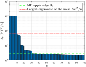
(a)

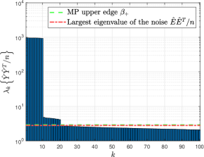
(b)

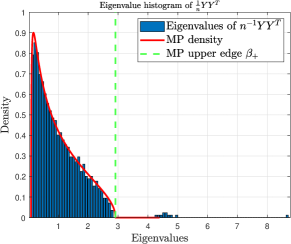
(c)

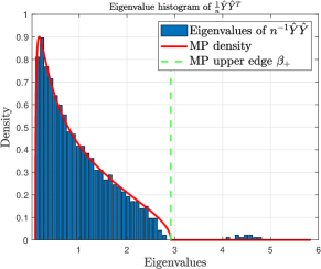
(d)

Figure 1: The spectrum of the original data (panels (a) and (c)) and after applying Algorithm 1 (panels (b) and (d)), where $m=1000$, $n=2000$, and $r=20$. The signal $X$ consists of $10$ strong components and $10$ weak components. The noise matrix $E$ is homoskedastic almost everywhere – except for the last $5$ rows and $5$ columns where the noise is abnormally strong.

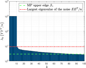
(a)

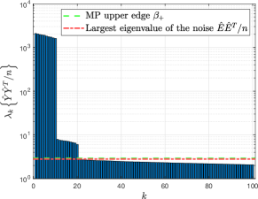
(b)

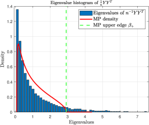
(c)

(d)

Figure 2: The spectrum of the original data (panels (a) and (c)) and after applying Algorithm 1 (panels (b) and (d)), where $m=1000$, $n=2000$, and $r=20$. The signal $X$ is identical to the one in the setting of Figure 1. The noise matrix $E$ is generated as Gaussian heteroskedastic, where $S_{ij}$ varies considerably across the rows and columns.

It is evident that in the first simulated scenario (Figures 1a and 1c), the bulk of the eigenvalues of $YY^{T}/n$ is well-approximated by the MP law since the noise is mostly homoskedastic. However, the severely corrupted rows and columns contribute $10$ significant components to the spectrum of the data. In this case, the first $10$ eigenvalues of $YY^{T}/n$ correspond to the strong signal components in the data, the next $10$ eigenvalues correspond to the $5$ noisy columns and $5$ noisy rows (in this order), and the last $10$ eigenvalues correspond to the weak signal components. Notably, there are $30$ eigenvalues of $YY^{T}/n$ that exceed the MP upper edge, while the signal’s rank is only $20$. Ideally, we would like to detect and recover all $20$ signal components (weak and strong) while filtering out the $10$ components arising from the corrupted rows and columns. However, this cannot be achieved by thresholding the singular values since the corrupted rows and columns are stronger in magnitude than the weak signal components. For the second simulated scenario (Figures 2a and 2c), we see that the bulk of the eigenvalues no longer fits the MP law and is much more spread out. In particular, the noise covers the weak signal components completely, prohibiting their detection and recovery via traditional approaches. Hence, relying on the spectrum of the observed data for signal detection and recovery can be restrictive under heteroskedastic noise. This challenge remains valid even if the eigenvalue density of $EE^{T}/n$ and its largest eigenvalue are known or can be inferred from the data; see, e.g., [46, 20, 13, 36, 28, 55].

Instead of using the spectrum of the observed data directly for signal detection and recovery, an alternative approach is to first normalize the data appropriately to stabilize the behavior of the noise. In the literature on robust covariance estimation under heavy-tailed distributions, it is well known that reweighting the data – by putting less weight on extremal observations – can lead to substantial improvement in recovery accuracy [57, 63, 22]. Data normalizations were also proposed and analyzed in [41, 26, 20, 27] under one-side heteroskedasticity, i.e., across the rows (observations) or columns (features). The results therein show that applying a suitable linear transformation to the heteroskedastic dimension (either the rows or the columns) can be highly beneficial for covariance estimation and matrix denoising. To account for more general variance patterns, [42] and [39] recently considered normalizing the data by scaling the rows and columns simultaneously. Specifically,

$$\widetilde{Y}=(D\{\mathbf{{x}}\})^{-1/2}Y(D\{\mathbf{{y}}\})^{-1/2}=\widetilde{X}+\widetilde{E},$$ (2)

where $\mathbf{x}\in\mathbb{R}^{m}$ and $\mathbf{y}\in\mathbb{R}^{n}$ are positive vectors, $D\{\nu\}$ is a diagonal matrix with $\nu$ on its main diagonal, and $\widetilde{X}=(D\{\mathbf{{x}}\})^{-1/2}X(D\{\mathbf{{y}}\})^{-1/2}$ is the scaled signal while $\widetilde{E}=(D\{\mathbf{{x}}\})^{-1/2}E(D\{\mathbf{{y}}\})^{-1/2}$ is the scaled noise. Notably, if the noise variance matrix is given by $S=\mathbf{x}\mathbf{y}^{T}$, which allows for heteroskedasticity across both rows and columns, then the normalization (2) makes the noise $\widetilde{E}$ completely homoskedastic with variance one.

The case of Gaussian heteroskedastic noise with $S=\mathbf{x}\mathbf{y}^{T}$ was considered in [42]. It was shown that in a suitable spiked model where the signal is sufficiently generic and delocalized, the normalization (2) enhances the spectral signal-to-noise ratio, namely, it increases the ratios between the signal’s singular values and the operator norm of the noise. Then, to improve signal recovery, [42] applied a spectral denoiser to $\widetilde{Y}$ that is optimally tuned for recovering $X$, followed by unscaling the rows and columns of the denoised matrix. If the noise variance matrix $S=\mathbf{x}\mathbf{y}^{T}$ is unknown, [42] proposed to estimate $\mathbf{x}$ and $\mathbf{y}$ directly from the magnitudes of the rows and columns of the data, i.e., from the sums of $Y_{ij}^{2}$ across the rows and columns. This approach relies on the assumption that $S=\mathbf{x}\mathbf{y}^{T}$ and requires the signal $X$ to be sufficiently weak compared to the noise $E$ and spread out across the entries.

In [39], the authors proposed to use the normalization (2) for rank estimation under heteroskedastic noise, utilizing the fact that the scaled signal $\widetilde{X}$ perseveres the rank of the original signal $X$. It was shown that for general variance matrices $S$ (not necessarily of the form $S=\mathbf{x}\mathbf{y}^{T}$), the normalization (2) can still enforce the standard spectral behavior of homoskedastic noise, namely the MP law for the spectrum of $\widetilde{E}\widetilde{E}^{T}/n$ and the convergence of its largest eigenvalue to the MP upper edge. The main idea is that by scaling the rows and columns of $S$ judiciously, we can control its average entry in each row and each column [53, 52]. Specifically, the normalization (2) can make the average entry in each row and each column of $\mathbb{E}[\widetilde{E}_{ij}^{2}]$ precisely one. This property is sufficient to enforce the spectral behavior of homoskedastic noise under non-restrictive conditions (see Proposition 4.1 in [39]). Then, the rank of $X$ is estimated simply by comparing the eigenvalues of $\widetilde{Y}\widetilde{Y}^{T}/n$ to the MP upper edge $(1+\sqrt{m/n})^{2}$. It was demonstrated in [39] that this method can accurately estimate the rank in challenging regimes, including in severe heteroskedasticity with general variance patterns and when strong signal components are present in the data. If $S$ is known, then the required scaling factors $\mathbf{x}$ and $\mathbf{y}$ can be obtained from $S$ by the Sinkhorn-Knopp algorithm [53, 52]. Otherwise,  [39] derived a procedure to estimate the required $\mathbf{x}$ and $\mathbf{y}$ from the data under the assumption that the variance of $Y_{ij}$ is a quadratic polynomial in its mean. This assumption holds for data sampled from prototypical count and nonnegative random variables such as Poisson, binominal, negative binomial, and Gamma [45].

1.1 Our results and contributions

In this work, we develop a data-driven version of the normalization (2) and utilize it for improved detection and recovery of low-rank signals under general heteroskedastic noise. Similarly to [42] and [39], the scaling factors $\mathbf{x}$ and $\mathbf{y}$ in our setting are designed to equalize the average noise variance across the rows and columns, i.e., make the average entry of $\widetilde{S}=(\mathbb{E}[\widetilde{E}_{ij}^{2}])=D^{-1}\{\mathbf{x}\}SD^{-1}\{\mathbf{y}\}$ in each row and each column to be precisely one. However, distinctly from [42] and [39], our approach allows us to estimate the required $\mathbf{x}$ and $\mathbf{y}$ directly from the observed data $Y$ in a broad range of settings without prior knowledge on the signal or the noise. Specifically, our main contribution is to derive estimators for $\mathbf{x}$ and $\mathbf{y}$ that support general distributions of the noise entries $E_{ij}$, diverse patterns of the variance $S_{ij}$ across the rows and columns, and a possibly strong signal $X$ that is localized in a subset of the entries; see Section 2. Then, relying on the normalization (2) with our estimated scaling factors, we propose suitable techniques for signal detection and recovery that adapt to general heteroskedastic noise. We provide theoretical justification for our proposed techniques and demonstrate their advantages in simulations; see Section 3. In Section 4, we exemplify the favorable performance of our normalization procedure on real data from single-cell RNA sequencing and spatial transcriptomics. Lastly, in Section 5, we discuss our results and some future research directions.

Our proposed data normalization procedure is described in Algorithm 1 below, where $\hat{\mathbf{x}}$ and $\hat{\mathbf{y}}$ denote our estimators for $\mathbf{x}$ and $\mathbf{y}$, respectively. The advantage of this procedure is demonstrated in Figures 1 and 2, where we compare the spectrum of the observed data in the two simulated scenarios discussed previously (in the context of the challenges posed by heteroskedastic noise) to the spectrum after Algorithm 1, i.e., $\hat{Y}=(D\{\mathbf{\hat{x}}\})^{-1/2}Y(D\{\mathbf{\hat{y}}\})^{-1/2}$, where we denote the normalized noise as $\hat{E}=(D\{\mathbf{\hat{x}}\})^{-1/2}E(D\{\mathbf{\hat{y}}\})^{-1/2}$. It is evident that in the first scenario, our proposed normalization removes the spurious eigenvalues arising from the severely corrupted rows and columns. As a consequence, only the true signal components exceed the MP upper edge. In the second scenario, our proposed normalization lowers the noise level in the spectrum and reveals the weak signal components under the noise. In both scenarios, our proposed normalization stabilizes the spectral behavior of the noise. In particular, the bulk of the eigenvalues after normalization is described accurately by the MP density, and moreover, the largest eigenvalue of $\hat{E}\hat{E}/n$ is very close to the MP upper edge, which is much smaller than the largest eigenvalue of $EE^{T}/n$ before normalization. Notably, our approach accurately infers the noise levels in the rows and columns of the data despite the fact that the signal is much stronger than the noise (due to the presence of the strong signal components). Indeed, in our simulation, the magnitude of the signal is $\|X\|_{F}^{2}\approx 10\times 10^{3}n=2\times 10^{7}$, which is $10$ times larger than the magnitude of the noise $\mathbb{E}\|E\|_{F}^{2}\approx mn=2\times 10^{6}$.

Algorithm 1 The Dyson Equalizer

1:Input: Data matrix $Y\in\mathbb{R}^{m\times n}$ with $m\leq n$ and no rows or columns that are entirely zero.

2:Compute the SVD of $Y$ and let the columns of $U\in\mathbb{R}^{m\times m}$, columns of $V\in\mathbb{R}^{n\times n}$, and $\{\sigma_{k}\}_{k=1}^{m}$ denote the left singular vectors, right singular vectors, and singular values of $Y$, respectively.

3:Set $\eta$ as the median singular value of $Y$, i.e., $\eta=\operatorname{Median}\{\sigma_{1},\ldots,\sigma_{m}\}$.

4:Compute the vectors $\hat{\mathbf{g}}^{(1)}\in\mathbb{R}^{m}$ and $\hat{\mathbf{g}}^{(2)}\in\mathbb{R}^{n}$ given by

$$\hat{\mathbf{g}}_{i}^{(1)}=\sum_{k=1}^{m}\frac{\eta}{\sigma_{k}^{2}+\eta^{2}}U_{ik}^{2},\qquad\qquad\hat{\mathbf{g}}_{j}^{(2)}=\frac{1}{\eta}+\sum_{k=1}^{m}\left(\frac{\eta}{\sigma_{k}^{2}+\eta^{2}}-\frac{1}{\eta}\right)V_{jk}^{2},$$ (3)

for all $i\in[m]$ and $j\in[n]$.

5:Compute the vectors $\hat{\mathbf{x}}\in\mathbb{R}^{m}$ and $\hat{\mathbf{y}}\in\mathbb{R}^{n}$ according to

$$\hat{\mathbf{x}}_{i}=\frac{1}{\sqrt{m-\eta\|\hat{\mathbf{g}}^{(1)}\|_{1}}}\left(\frac{1}{\hat{\mathbf{g}}_{i}^{(1)}}-\eta\right),\qquad\qquad\hat{\mathbf{y}}_{j}=\frac{1}{\sqrt{n-\eta\|\hat{\mathbf{g}}^{(2)}\|_{1}}}\left(\frac{1}{\hat{\mathbf{g}}_{j}^{(2)}}-\eta\right),$$ (4)

for all $i\in[m]$ and $j\in[n]$.

6:Form the normalized data matrix $\hat{Y}=(D\{\mathbf{\hat{x}}\})^{-1/2}Y(D\{\mathbf{\hat{y}}\})^{-1/2}$.

Our approach for estimating the scaling factors $\mathbf{x}$ and $\mathbf{y}$ relies on recent results in random matrix theory [2, 14]. These results establish that the main diagonal of the resolvent of the noise (see eq. (6)) concentrates around the solution to a nonlinear equation known as the Dyson equation (see eq. (7)). Importantly, this phenomenon is universal, i.e., it holds for general noise distributions, where the Dyson equation and its solution depend only on the variance matrix $S$; see Section 2.1. Building on these results, we show that in a broad range of settings, there is a tractable relation between the resolvent of the observed data (see eq. (14)) and the variance pattern of the noise. To the best of our knowledge, our approach is the first to exploit this relation to infer the noise variance structure in the signal+noise model (1). Below is a detailed account of our results and contributions.

We begin by considering the case of a rank-one variance matrix $S=\mathbf{x}\mathbf{y}^{T}$ in section 2.2. We observe that in this case, there is an explicit formula for $\mathbf{x}$ and $\mathbf{y}$ in terms of the solution to the aforementioned Dyson equation; see Proposition 2. Since we do not have access to this solution (as it depends on $S$, which is unknown), we propose to estimate it directly from the main diagonal of the resolvent of the observed data, which acts as a surrogate to the resolvent of the noise. One of our main technical contributions is to show that the resolvent of the data is robust to the presence of the low-rank signal $X$ regardless of the signal’s magnitude; see Theorem 6 and Corollaries 7 and 8. Intuitively, this favorable property follows from the fact that the resolvent of the data is inversely proportional to the singular values of $Y$ (see Proposition 3 and its proof). Hence, strong signal components that correspond to large singular values in the data have a limited influence on the resolvent. Building on these results, we provide estimators for $\mathbf{x}$ and $\mathbf{y}$ via the resolvent of the data and characterize their accuracy in terms of the dimensions of the matrix and the localization level of the singular vectors of the signal $X$; see Theorem 9. Our theoretical guarantees here are non-asymptotic, allow $m$ and $n$ to grow disproportionally, and support regimes where the singular vectors of $X$ concentrate in a vanishingly small number of entries, while the signal’s magnitude can be arbitrary. The convergence of our estimators to the true scaling factors in these settings is demonstrated numerically in Figure 3 in Section 2.2.

In Section 2.3, we extend the results described above to support general variance matrices $S$ beyond rank-one. Similarly to [39], we rely on the fact that any positive variance matrix $S$ can be written as $S=D(\mathbf{x})\widetilde{S}D(\mathbf{y})$, where $\widetilde{S}$ is doubly regular, meaning that average entry in each row and each column of $\widetilde{S}$ is $1$; see Definition 10 and Proposition 11. We investigate which variance matrices $S$ allow us to accurately estimate $\mathbf{x}$ and $\mathbf{y}$ using the procedure developed previously in Section 2.2. We show that the same procedure can be used to estimate $\mathbf{x}$ and $\mathbf{y}$ accurately if $\widetilde{S}$ is sufficiently incoherent with respect to $\mathbf{x}$ and $\mathbf{y}$; see Theorem 14 and Lemma 13. We demonstrate that this incoherence condition is satisfied by several prototypical random constructions of $\widetilde{S}$, in which case $S$ need not be rank-one or even low-rank. We demonstrate numerically the convergence of our proposed estimators in this case in Figure 4 in Section 2.3.

In Section 3, we utilize our proposed normalization for automating and improving signal detection and recovery under heteroskedastic noise. We first consider the task of rank estimation in Section 3.1. We establish that under suitable conditions, our proposed normalization from Algorithm 1 enforces the standard spectral behavior of homoskedastic noise, i.e., the MP law for the eigenvalue density of $\hat{E}\hat{E}/n$ and the convergence of its largest eigenvalue to the MP upper edge; see Theorem 15. This fact allows for a simple and reliable procedure for rank estimation by comparing the eigenvalues of $\hat{Y}\hat{Y}^{T}/n$ to the MP upper edge; see Algorithm 2 in Section 3.1 and the relevant discussion. We also show that our proposed normalization can significantly reduce the operator norm of the noise and enhance the spectral signal-to-noise ratio, thereby improving the detection of weak signal components under heteroskedasticity; see Figure 5 and the discussion in Section 3.1.

We proceed in Section 3.2 to address the task of recovering the signal $X$. Instead of the traditional approach of thresholding the singular values of the observed data $Y$, we propose to threshold the singular values of the data after normalization, i.e., $\hat{Y}$ from Algorithm 1, followed by unscaling the rows and columns correspondingly; see Algorithm 3 in Section 3.2. We show that this approach arises naturally from maximum-likelihood estimation of $X$ under Gaussian heteroskedastic noise with variance $S=\mathbf{x}\mathbf{y}^{T}$. For Gaussian noise with a more general variance matrix $S$ (beyond rank-one), we show that the proposed approach provides an appealing approximation to the true maximum-likelihood estimation problem; see Proposition 16 and the relevant discussion. Importantly, our approach is applicable beyond Gaussian noise and is naturally interpretable; it is equivalent to solving a weighted low-rank approximation problem [54] – seeking the best low-rank approximation to the data in a weighted least-squares sense – where the weights adaptively penalize the rows and columns according to their inherent noise levels. As a refined alternative to thresholding the singular values after our proposed normalization, we also consider the denoising technique of [41]. We demonstrate in simulations that our normalization, when combined with singular value thresholding or the denoising technique of [41], can substantially improve the recovery accuracy of the signal $X$ over alternative approaches under heteroskedasticity; see Figure 6 and the corresponding text.

Lastly, in Section 4, we exemplify our proposed normalization on real data from single-cell RNA sequencing and spatial transcriptomics, comparing our approach to the method of [39]. We demonstrate that our proposed normalization and the method of [39] both result in accurate fits to the MP law when applied to the raw count data; see Figures 7a–7f. However, after applying a certain transformation to the data that is commonly used for downstream analysis, the method of [39] provides unsatisfactory performance, whereas our approach still provides an excellent fit to the MP law; see Figures 7g–7l. The reason for this advantage is that our approach supports general noise distributions and is agnostic to the signal, whereas the method of [39] relies on a quadratic relation between the mean and the variance of the data entries, which is hindered by the transformation.

2 Method derivation and analysis

2.1 Preliminaries: the noise resolvent and the quadratic Dyson equation

We begin by defining $\mathcal{E},\mathcal{S}\in\mathbb{R}^{(m+n)\times(m+n)}$ as the symmetrized versions of $E$ and $S$, respectively, according to

$$\mathcal{E}=\begin{bmatrix}\mathbf{0}_{m\times m}&E\\ E^{T}&\mathbf{0}_{n\times n}\end{bmatrix},\qquad\qquad\mathcal{S}=\begin{bmatrix}\mathbf{0}_{m\times m}&S\\ S^{T}&\mathbf{0}_{n\times n}\end{bmatrix},$$ (5)

where $\mathbf{0}_{m\times m}$ and $\mathbf{0}_{n\times n}$ are $m\times m$ and $n\times n$ zero matrices, respectively. Next, the resolvent of $\mathcal{E}$ is defined as the complex-valued random matrix $R(z)\in\mathbb{C}^{(m+n)\times(m+n)}$ given by

$$R(z)=(\mathcal{E}-zI)^{-1},$$ (6)

where $I$ is the identity matrix and $z\in\mathbb{H}^{+}$ is point in the complex upper half plane $\mathbb{H}^{+}$. A fundamental fact underpinning our approach is that in a broad range of settings, the main diagonal of $R(z)$ concentrates around the solution $\mathbf{f}\in\mathbb{C}^{m+n}$ to the deterministic vector-valued equation

$$z+\mathcal{S}\mathbf{f}=-\frac{1}{\mathbf{f}},$$ (7)

for any $z\in\mathbb{H}^{+}$; see [14, 2] and references therein. For simplicity of presentation, we use a standard fraction notation, e.g., in the right-hand side of (7), to denote entrywise division whenever vectors are involved. The equation (7) is known as the quadratic Dyson equation and has been extensively studied in the literature on random matrix theory. The following proposition guarantees the existence and uniqueness of the solution $\mathbf{f}$ and states several useful properties (see [1]).

Proposition 1.

There exists a unique holomorphic function $\mathbf{f}:\mathbb{H}^{+}\rightarrow\mathbb{C}^{m+n}$ that solves (7) for all $z\in\mathbb{H}^{+}$. Moreover, $\operatorname{Im}\{\mathbf{f}(z)\}>0$ for all $z\in\mathbb{H}^{+}$ and $\operatorname{Re}\{\mathbf{f}(z)\}$ is an odd function of $\operatorname{Re}\{z\}$.

In what follows, we focus on the restriction of $\mathbf{f}$ to the upper half of the imaginary axis, i.e., $z=\imath\eta$ for $\eta>0$. In this case, Proposition 1 asserts that the real part of $\mathbf{f}$ vanishes and its imaginary part is strictly positive, hence

$$\mathbf{f}(\imath\eta)=\imath\mathbf{g}(\eta),$$ (8)

where $\mathbf{g}(\eta)\in\mathbb{R}^{m+n}$ is a positive vector for all $\eta>0$. By plugging (8) into the Dyson equation for $z=\imath\eta$ and taking the imaginary part of both sides, we see that $\mathbf{g}$ satisfies the vector-valued equation

$$\eta+\mathcal{S}\mathbf{g}=\frac{1}{\mathbf{g}}.$$ (9)

Note that according to the definition of $\mathcal{S}$ in (5), the equation (9) can also be written as the system of coupled equations

$$\eta+{S}\mathbf{g}^{(2)}=\frac{1}{\mathbf{g}^{(1)}},\qquad\qquad\eta+{S^{T}}\mathbf{g}^{(1)}=\frac{1}{\mathbf{g}^{(2)}},$$ (10)

where $\mathbf{g}^{(1)}=[\mathbf{g}_{1},\ldots,\mathbf{g}_{m}]^{T}$ and $\mathbf{g}^{(2)}=[\mathbf{g}_{m+1},\ldots,\mathbf{g}_{m+n}]^{T}$. The system of equations in (10) involves only real-valued and strictly positive quantities, making it particularly convenient for our subsequent derivation and analysis.

2.2 Variance matrices $S$ with rank one

We begin by considering the case of a rank-one variance matrix, i.e.,

Assumption 1.

$S=\mathbf{x}\mathbf{y}^{T}$ for positive $\mathbf{x}\in\mathbb{R}^{m}$ and $\mathbf{y}\in\mathbb{R}^{n}$.

As mentioned in the introduction, in this case, the normalization of the rows and columns in (2) makes the noise completely homoskedastic with noise variance $1$, i.e., $\mathbb{E}[{\widetilde{E}}_{ij}^{2}]=1$ for all $i\in[m]$ and $j\in[n]$. In what follows, we address the task of estimating $\mathbf{x}$ and $\mathbf{y}$ directly from the data matrix $Y$. We begin by deriving our proposed estimators and proceed to analyze their convergence to $\mathbf{x}$ and $\mathbf{y}$. Our main result in this section is Theorem 9, which provides probabilistic error bounds for our proposed estimators under suitable conditions.

2.2.1 Method derivation

To derive our estimators for $\mathbf{x}$ and $\mathbf{y}$, we observe that under Assumption 1, the vectors $\mathbf{x}$ and $\mathbf{y}$ can be written explicitly in terms of $\mathbf{g}^{(1)}$ and $\mathbf{g}^{(2)}$ from (10) up to a trivial scalar ambiguity. Specifically, we have the following proposition, whose proof can be found in Appendix E.

Proposition 2.

Under Assumption 1, we have

$$\mathbf{x}=\frac{\alpha}{\sqrt{m-\eta\|\mathbf{g}^{(1)}\|_{1}}}\left(\frac{1}{\mathbf{g}^{(1)}}-\eta\right),\qquad\mathbf{y}=\frac{\alpha^{-1}}{\sqrt{n-\eta\|\mathbf{g}^{(2)}\|_{1}}}\left(\frac{1}{\mathbf{g}^{(2)}}-\eta\right),\qquad\alpha=\sqrt{\frac{\mathbf{x}^{T}\mathbf{g}^{(1)}}{\mathbf{y}^{T}\mathbf{g}^{(2)}}}.$$ (11)

The scalar ambiguity in Proposition 2 stems from the fact that $\mathbf{x}$ and $\mathbf{y}$ can always be replaced with $\alpha^{-1}\mathbf{x}$ and $\alpha\mathbf{y}$, respectively, for any $\alpha>0$, resulting in the same noise variance matrix $S=\mathbf{x}\mathbf{y}^{T}$. To settle this ambiguity, we set $\alpha=1$ by requiring that

$$\mathbf{x}^{T}\mathbf{g}^{(1)}=\mathbf{y}^{T}\mathbf{g}^{(2)},$$ (12)

which can be assumed to hold without loss of generality.

We propose to estimate $\mathbf{x}$ and $\mathbf{y}$ by first estimating $\mathbf{g}^{(1)}$ and $\mathbf{g}^{(2)}$ from the observed data and then utilizing the formulas in Proposition 2 with $\alpha=1$. As mentioned in Section 2.1, under suitable conditions (see, e.g., [2, 14]), the main diagonal of the noise resolvent $R(z)$ concentrates around the solution $\mathbf{f}(z)$ to the Dyson equation (7). Since $\mathbf{g}(\eta)=\operatorname{Im}\{\mathbf{f}(\imath\eta)\}$ according to (8), we expect the imaginary part of the main diagonal of the noise resolvent $R(\imath\eta)$ to approximate $\mathbf{g}(\eta)$. However, since we do not have direct access to the noise resolvent, we replace it with the resolvent constructed analogously from the data. To this end, we define $\mathcal{Y}\in\mathbb{R}^{(m+n)\times(m+n)}$ as the symmetrized version of the data matrix $Y$, i.e.,

$$\mathcal{Y}=\begin{bmatrix}\mathbf{0}_{m\times m}&Y\\ Y^{T}&\mathbf{0}_{n\times n}\end{bmatrix},$$ (13)

and denote the resolvent of $\mathcal{Y}$ by $\mathcal{R}(z)\in\mathbb{C}^{(m+n)\times(m+n)}$, namely

$$\mathcal{R}(z)=(\mathcal{Y}-zI)^{-1},$$ (14)

for $z\in\mathbb{H}^{+}$. We then estimate $\mathbf{g}(\eta)$ from the imaginary part of the main diagonal of the data resolvent $\mathcal{R}(\imath\eta)$ according to

$$\hat{\mathbf{g}}_{i}(\eta)=\operatorname{Im}\{\mathcal{R}_{ii}(\imath\eta)\},$$ (15)

for all $i\in[m+n]$. For notational convenience, we define the estimates of $\mathbf{g}^{(1)}$ and $\mathbf{g}^{(2)}$ separately as $\hat{\mathbf{g}}^{(1)}=[\hat{\mathbf{g}}_{1},\ldots,\hat{\mathbf{g}}_{m}]^{T}$ and $\hat{\mathbf{g}}^{(2)}=[\hat{\mathbf{g}}_{m+1},\ldots,\hat{\mathbf{g}}_{m+n}]^{T}$, respectively, and omit the explicit dependence on $\eta$.

The following proposition, whose proof can be found in Appendix F, shows that $\hat{\mathbf{g}}^{(1)}$ and $\hat{\mathbf{g}}^{(2)}$ have simple formulas in terms of the SVD of $Y$ (recalling our assumption that $m\leq n$). In particular, these formulas justify steps 2 and 4 in Algorithm 1.

Proposition 3.

Let the columns of $U\in\mathbb{R}^{m\times m}$, the columns of $V\in\mathbb{R}^{n\times n}$, and $\{\sigma_{k}\}_{k=1}^{m}$ denote the left singular vectors, right singular vectors, and singular values of $Y$, respectively. Then,

$$\hat{\mathbf{g}}_{i}^{(1)}=\sum_{k=1}^{m}\frac{\eta}{\sigma_{k}^{2}+\eta^{2}}U_{ik}^{2},\qquad\qquad\hat{\mathbf{g}}_{j}^{(2)}=\frac{1}{\eta}+\sum_{k=1}^{m}\left(\frac{\eta}{\sigma_{k}^{2}+\eta^{2}}-\frac{1}{\eta}\right)V_{jk}^{2},$$ (16)

for all $i\in[m]$ and $j\in[n]$.

As we shall see in our analysis, an important property of the estimator $\hat{\mathbf{g}}$ of $\mathbf{g}$ is that it is not sensitive to the presence of a possibly strong low-rank signal $X$. This is one of the main advantages of using the data resolvent to infer the structure of the noise variance, as opposed to, e.g., computing the empirical variances of the data matrix $Y$ across its rows and columns, which can be highly sensitive to the presence of strong components in the signals.

Equipped with an estimator of $\mathbf{g}$, we propose to estimate $\mathbf{x}$ and $\mathbf{y}$ by replacing $\mathbf{g}^{(1)}$ and $\mathbf{g}^{(2)}$ in (11) with their estimates $\hat{\mathbf{g}}^{(1)}$ and $\hat{\mathbf{g}}^{(2)}$, respectively, taking $\alpha=1$. Specifically, we define

$$\hat{\mathbf{x}}=\frac{1}{\sqrt{m-\eta\|\hat{\mathbf{g}}^{(1)}\|_{1}}}\left(\frac{1}{\hat{\mathbf{g}}^{(1)}}-\eta\right),\qquad\qquad\hat{\mathbf{y}}=\frac{1}{\sqrt{n-\eta\|\hat{\mathbf{g}}^{(2)}\|_{1}}}\left(\frac{1}{\hat{\mathbf{g}}^{(2)}}-\eta\right),$$ (17)

which agrees with Step 5 in Algorithm 1. The following proposition, whose proof can be found in Appendix G, establishes the well-posedness of the formulas in (17) and the normalization (2) when replacing $\mathbf{x}$ and $\mathbf{y}$ with $\hat{\mathbf{x}}$ and $\hat{\mathbf{y}}$, respectively. In particular, this proposition justifies our requirement at the beginning of Algorithm 1.

Proposition 4.

The vector $\hat{\mathbf{g}}$ from (15) is positive for any $\eta>0$. Further, if $Y$ is not the zero matrix, i.e., $Y\neq\mathbf{0}_{m\times n}$, then $\hat{\mathbf{x}}$ and $\hat{\mathbf{y}}$ from (17) are nonnegative vectors for any $\eta>0$, where $\hat{\mathbf{x}}_{i}=0$ ($\hat{\mathbf{y}}_{j}=0$) if and only if the $i$’th row ($j$’th column) of $Y$ is entirely zero.

Lastly, while our derivation in this section does not restrict the value of $\eta>0$, we propose in practice to set $\eta$ as the median singular value of $Y$; see step 3 in Algorithm 1. The purpose of this choice is to adapt our procedure to the global scaling of the noise in the data. In particular, this choice of $\eta$ enforces a certain scaling of the noise that is required for our analysis in the next section; see Assumptions 2 and 5 in the next section and the discussion in Appendix B.

2.2.2 Convergence analysis

For our analysis in this section and subsequent ones, we consider $\eta$ and the signal’s rank $r$ as fixed global constants. All other quantities in our setup, such as the matrix dimensions $m$ and $n$, the distribution of the noise entries $E_{ij}$, and the signal $X$ (its $r$ leading singular values and vectors) can be arbitrary, pending that they satisfy the requirements imposed by our assumptions detailed below. Therefore, in what follows, all constants appearing in our results may depend only on $\eta$, $r$, and the relevant global constants defined in our assumptions.

To formally state the relation between $\mathbf{g}$ from (9) and the noise resolvent $R(z)$, we require all moments of the scaled noise variables $\sqrt{n}E_{ij}$ to be upper bounded by global constants. That is,

Assumption 2.

There exist global constants $\{\mu_{q}\}_{q=1}^{\infty}$ such that $\mathbb{E}|\sqrt{n}E_{ij}|^{q}\leq\mu_{q}$ for all $i\in[m]$, $j\in[n]$, $q\in\mathbb{N}$.

Assumption 2 is non-restrictive and covers many standard noise models, including all sub-Gaussian and sub-Exponential distributions [58]. We now have the following lemma, which characterizes the relation between the noise resolvent on the imaginary axis, i.e., $R(\imath\eta)$, and the vector $\mathbf{g}$ from (9).

Lemma 5.

Under Assumption 2, for any $\epsilon>0$ there exist $C^{{}^{\prime}},c^{{}^{\prime}}(t)>0$ such that for all deterministic unit vectors $\mathbf{a},\mathbf{b}\in\mathbb{C}^{m+n}$ (i.e., $\|\mathbf{a}\|_{2}=\|\mathbf{b}\|_{2}=1$), we have

$$\left|\mathbf{a}^{T}\left[R(\imath\eta)-D\{\imath\mathbf{g}(\eta)\}\right]\mathbf{b}\right|\leq C^{{}^{\prime}}n^{\epsilon-1/2},$$ (18)

with probability at least $1-c^{{}^{\prime}}(t)n^{-t}$, for all $t>0$.

The proof of Lemma 5 can be found in Appendix D and follows directly from the results in [14] adapted to our setting. Lemma 5 establishes the concentration of bilinear forms of the noise resolvent evaluated on the imaginary axis in terms of the deterministic vector $\mathbf{g}$. In particular, it asserts that under Assumption 2 and for large $n$ (the long dimension), the noise resolvent $R(\imath\eta)$ behaves like a diagonal matrix whose main diagonal is $\imath\mathbf{g}$. We mention that under Assumption 2, the entries of $\mathbf{g}$ are always lower bounded away from zero by a global constant (which may depend on $\eta$); see Lemma 17 in Appendix C.1. Therefore, we have that $\operatorname{Im}\{R_{ii}(\imath\eta)\}\sim\mathbf{g}_{i}(\eta)$ almost surely as $n\rightarrow\infty$ for all $i\in[m+n]$, where the convergence rate is almost $n^{-1/2}$. Consequently, for large $n$, the main diagonal of the noise resolvent provides an accurate approximation to the solution $\mathbf{g}$ to the Dyson equation (9) on the imaginary axis. We note that the statement in Lemma 5 on the concentration of bilinear forms of a matrix is stronger than a statement on the concentration of the entries. Indeed, the former implies the latter but not vice-versa. This stronger statement is required for our key result below on the concentration of the main diagonal of the data resolvent.

Let us denote the (compact) SVD of the signal matrix $X$ as

$$X=\widetilde{U}D\{s_{1},\ldots,s_{r}\}\widetilde{V}^{T},$$ (19)

where $\widetilde{U}\in\mathbb{R}^{m\times r}$, $\widetilde{V}\in\mathbb{R}^{n\times r}$, and $s_{1},\ldots,s_{r}$ stand for the left singular vectors, right singular vectors, and singular values of $X$, respectively. To analyze the behavior of $\hat{\mathbf{g}}$ in the signal+noise model (1), we make the simplifying assumption that all nonzero signal singular values are identical and equal to $s$, namely

Assumption 3.

$s_{1}=\ldots=s_{r}=s>0$.

We now have the following theorem, which characterizes the concentration of $\hat{\mathbf{g}}$ around $\mathbf{g}$ in terms of the long dimension $n$ and the SVD of the signal $X$.

Theorem 6.

Under Assumptions 2 and 3, for any $\epsilon>0$ there exist $C_{1}^{{}^{\prime}},C_{2}^{{}^{\prime}},C_{3}^{{}^{\prime}},c^{{}^{\prime}}(t)>0$ such that

$$|\hat{\mathbf{g}}_{i}^{(1)}-{\mathbf{g}}_{i}^{(1)}| \leq C_{1}^{{}^{\prime}}n^{\epsilon-1/2}+\frac{C_{2}^{{}^{\prime}}}{\sqrt{s^{-2}+C_{3}^{{}^{\prime}}}}\sum_{k=1}^{r}\widetilde{U}_{ik}^{2},$$ (20)

$$|\hat{\mathbf{g}}_{j}^{(2)}-{\mathbf{g}}_{j}^{(2)}| \leq C_{1}^{{}^{\prime}}n^{\epsilon-1/2}+\frac{C_{2}^{{}^{\prime}}}{\sqrt{s^{-2}+C_{3}^{{}^{\prime}}}}\sum_{k=1}^{r}\widetilde{V}_{jk}^{2},$$ (21)

for all $i\in[m]$ and $j\in[n]$ with probability at least $1-c^{{}^{\prime}}(t)n^{-t}$, for all $t>0$.

The proof of Theorem 6 can be found in Appendix H. The main idea therein is to utilize the Woodbury matrix identity together with Lemma 5 to show that the main diagonal of the data resolvent $\mathcal{R}(\imath\eta)$ concentrates around $\imath\mathbf{g}$ plus an error term. This additive error term has a special algebraic structure, which can be expressed in terms of the singular values of $X$ and bilinear forms involving $D\{\imath\mathbf{g}\}$ and the singular vectors of $X$. We then conduct a careful spectral analysis of this error term to prove the required result. It is important to note that Theorem 6 does not rely on Assumption 1. Consequently, the probabilistic bound in Theorem 6 does not depend on the structure of the noise variance matrix $S$. This fact will be important for our analysis in the next section involving general variance matrices.

From Theorem 6, we see that the probabilistic errors between $\hat{\mathbf{g}}$ and $\mathbf{g}$ in (20) and (21) have two terms. The first term depends only on the long data dimension $n$ and converges to zero with rate almost $n^{-1/2}$. The second term depends on the signal magnitude $s$ and the magnitude of the entries of the singular vectors $\widetilde{U}$ and $\widetilde{V}$. Evidently, if the signal is vanishingly small, i.e., $s\rightarrow 0$, then the second error term vanishes and, as expected from Lemma 5, $\hat{\mathbf{g}}$ approaches $\mathbf{g}$ with rate almost $n^{-1/2}$ (with probability rapidly approaching $1$). However, even if the magnitude of the signal $s$ is arbitrarily large, we always have

$$\frac{C_{2}^{{}^{\prime}}}{\sqrt{s^{-2}+C_{3}^{{}^{\prime}}}}\sum_{k=1}^{r}\widetilde{U}_{ik}^{2}\leq\frac{C_{2}^{{}^{\prime}}}{\sqrt{C_{3}^{{}^{\prime}}}}\sum_{k=1}^{r}\widetilde{U}_{ik}^{2},\qquad\frac{C_{2}^{{}^{\prime}}}{\sqrt{s^{-2}+C_{3}^{{}^{\prime}}}}\sum_{k=1}^{r}\widetilde{V}_{jk}^{2}\leq\frac{C_{2}^{{}^{\prime}}}{\sqrt{C_{3}^{{}^{\prime}}}}\sum_{k=1}^{r}\widetilde{V}_{jk}^{2},$$ (22)

which depends only on the singular vectors of $X$. Since each singular vector has unit Euclidean norm, we have the following immediate corollary of Theorem 6.

Corollary 7.

Under Assumptions 2 and 3, for any $\epsilon>0$ there exist $C^{{}^{\prime}},c^{{}^{\prime}}(t)>0$ such that

$$\frac{1}{m}\|\hat{\mathbf{g}}^{(1)}-\mathbf{g}^{(1)}\|_{1}\leq C^{{}^{\prime}}\max\left\{n^{\epsilon-1/2},m^{-1}\right\},\qquad\frac{1}{n}\|\hat{\mathbf{g}}^{(2)}-\mathbf{g}^{(2)}\|_{1}\leq C^{{}^{\prime}}n^{\epsilon-1/2},$$ (23)

with probability at least $1-c^{{}^{\prime}}(t)n^{-t}$, for all $t>0$.

Therefore, the average absolute error between $\hat{\mathbf{g}}^{(1)}$ and ${\mathbf{g}}^{(1)}$ always converges to zero as $n\rightarrow\infty$ with probability approaching $1$ and rate almost $n^{-1/2}$. This convergence does not depend on $m$ (the short dimension) nor the low-rank signal $X$. If $m$ also grows with $n$, then the average absolute error between $\hat{\mathbf{g}}^{(2)}$ and ${\mathbf{g}}^{(2)}$ also converges to zero (with probability approaching $1$). In this case, the convergence rate depends on the growth rate of $m$ with respect to $n$. Note that when $m,n\rightarrow\infty$, the convergence of the average absolute errors discussed above implies that almost all entries of $\hat{\mathbf{g}}$ converge to the corresponding entries of $\mathbf{g}$ with probability approaching $1$. In particular, the proportion of indices $i\in[m]$ and $j\in[n]$ for which the errors $|\hat{\mathbf{g}}_{i}^{(1)}-\mathbf{g}_{i}^{(1)}|$ and $|\hat{\mathbf{g}}_{j}^{(2)}-\mathbf{g}_{j}^{(2)}|$ do not converge to zero must be vanishing as $m,n\rightarrow\infty$ (otherwise, it would be a contradiction to the convergence of the average absolute errors). Therefore, the main diagonal of the data resolvent $\mathcal{R}(\imath\eta)$ is robust to the presence of the low-rank signal $X$ in the sense that for large $m$ and $n$, we can use it to accurately estimate almost all entries of $\mathbf{g}$ regardless of $X$ and its structure.

To proceed, it is convenient to have a stronger control of the element-wise errors between $\hat{\mathbf{g}}$ and $\mathbf{g}$. Specifically, it is desirable to guarantee the stochastic convergence of $\|\hat{\mathbf{g}}-\mathbf{g}\|_{\infty}$. To this end, we make the following assumption on the behavior of the singular vectors of $X$, where we use the notation $\|\cdot\|_{\infty}$ to represent the maximal absolute entry in a vector or a matrix.

Assumption 4.

There exist constants $\widetilde{C},\delta>0$ such that $\max\{\|\widetilde{U}\|_{\infty}^{2}$, $\|\widetilde{V}\|_{\infty}^{2}\}\leq\widetilde{C}n^{-\delta}$.

In other words, we require the maximal absolute entry in the singular vectors of $X$ to decay with some fractional power of $n$. Essentially, this is an assumption on the delocalization of the singular vectors of $X$. In particular, it prohibits the singular vectors from having too few non-zero entries, e.g., a fixed number of non-zeros or a logarithmically growing number of non-zeros with respect to $n$. However, the singular vectors can still be sparse or localized in a vanishingly small proportion of entries. For instance, suppose that each column of $\widetilde{U}$ has only $\lceil\sqrt{m}\rceil$ nonzero entries and each column of $\widetilde{V}$ has only $\lceil\sqrt{n}\rceil$ nonzero entries, where $\lceil\cdot\rceil$ denotes the ceiling function. For simplicity, suppose also that all nonzero entries in the singular vectors have identical absolute values. Then, $\max\{\|\widetilde{U}\|_{\infty}^{2}$, $\|\widetilde{V}\|_{\infty}^{2}\}\leq\max\{m^{-1/2},n^{-1/2}\}=m^{-1/2}$. In this case, if $m$ is proportional to $n$, Assumption 4 holds with $\delta=1/2$, implying that the proportion of nonzero entries in $\widetilde{U}$ and $\widetilde{V}$ vanish at rate $n^{-1/2}$, allowing for significant sparsity of the singular vectors. Alternatively, if, for example, $m$ is proportional to $\sqrt{n}$, then Assumption 4 holds with $\delta=1/4$. Generally, Assumption 4 allows the singular vectors of $X$ to be localized in subsets of entries with cardinality proportional to any fractional power of $n$. We remark that Assumption 4 requires $m$ to grow at least with some fractional power of $n$. Specifically, since we always have $\|\widetilde{U}\|_{\infty}^{2}\geq m^{-1}$, Assumption 4 implies that $m\geq n^{\delta}/\widetilde{C}$.

Combining Theorem 6 with Assumption 4, we get the following immediate corollary.

Corollary 8.

Under Assumptions 2,3,4, for any $\epsilon>0$ there exist $C^{{}^{\prime}},c^{{}^{\prime}}(t)>0$ such that

$$\left\|{\hat{\mathbf{g}}-\mathbf{g}}\right\|_{\infty}\leq C^{{}^{\prime}}\max\left\{n^{\epsilon-1/2},n^{-\delta}\right\},$$ (24)

with probability at least $1-c^{{}^{\prime}}(t)n^{-t}$, for all $t>0$.

Corollary 8 establishes the stochastic entrywise convergence of $\hat{\mathbf{g}}$ to $\mathbf{g}$ with rate that depends on the localization level of the singular vectors and the growth rate of $m$ with respect to $n$; see Assumption 4. For the example described in the text after Assumption 4, where $\delta=1/2$, the convergence rate of $\hat{\mathbf{g}}$ to $\mathbf{g}$ would remain almost $n^{-1/2}$. However, the convergence rate can be slower if $\delta$ is smaller, e.g., if the singular vectors are concentrated in a smaller number of entries of if $m$ is not proportional to $n$ and grows slower.

Next, we turn to establish the entrywise concentration of $\hat{\mathbf{x}}$ and $\hat{\mathbf{y}}$ around $\mathbf{x}$ and $\mathbf{y}$, respectively. To this end, we need two additional assumptions. First, we require that the noise variances $S_{ij}$ are lower bounded by a global constant divided by $n$, i.e.,

Assumption 5.

There exist a global constant $c>0$ such that $S_{ij}\geq{c}{n}^{-1}$ for all $i\in[m]$ and $j\in[n]$.

Therefore, together with Assumption 2, we require the noise variances to be lower and upper bounded according to $cn^{-1}\leq S_{ij}\leq\mu_{2}n^{-1}$. Since the constants $\mu_{2},c>0$ are arbitrary, e.g., $c=0.01$ and $\mu_{2}=100$, this boundedness requirement is not restrictive and allows the noise variances to differ substantially across the rows and columns of the data. We note that the global scaling of the noise $S_{ij}\propto n^{-1}$ is convenient for analysis but is not required in practice. In particular, we can enforce it automatically by our choice of $\eta$ in step 3 of Algorithm 1; see the discussion in Appendix B.

Our second assumption is that $m$ (the short dimension) grows sufficiently quickly with respect to $n$.

Assumption 6.

There exist global constants $\widetilde{C}_{2},\delta_{2}>0$ such that $m\geq\widetilde{C}_{2}\max\{n^{1/2+\delta_{2}},n^{1-\delta+\delta_{2}}\}$.

Assumption 6 requires that $m$ grows with a rate slightly faster than $\sqrt{n}$ and $n^{1-\delta}$, where the latter depends on the delocalization level of the signal’s singular vectors according to Assumption 4. Note that Assumption 6 is always satisfied if $m$ grows proportionally to $n$, i.e., if $\widetilde{C}_{2}n\leq m\leq n$ (since we can take any $\delta_{2}<\min\{1/2,\delta\}$), regardless of the singular vectors’ delocalization.

We now have the main result of this section, which provides probabilistic bounds on the relative entrywise deviations between the pairs $(\hat{\mathbf{x}},\hat{\mathbf{y}})$ and $(\mathbf{x},\mathbf{y})$, respectively.

Theorem 9.

Under Assumptions 2–5, for any $\epsilon>0$ there exist $C^{{}^{\prime}},c^{{}^{\prime}}(t)>0$ such that

$$\left\|\frac{\hat{\mathbf{x}}-\mathbf{x}}{\mathbf{x}}\right\|_{\infty}\leq C^{{}^{\prime}}\max\left\{n^{\epsilon-1/2},n^{-\delta}\right\},$$ (25)

with probability at least $1-c^{{}^{\prime}}(t)n^{-t}$, for all $t>0$. Furthermore, if Assumption 6 holds, then for any $\epsilon<\delta_{2}$,

$$\left\|\frac{\hat{\mathbf{y}}-\mathbf{y}}{\mathbf{y}}\right\|_{\infty}\leq C^{{}^{\prime}}\max\left\{\frac{n^{\epsilon+1/2}}{m},\frac{n^{1-\delta}}{m}\right\},$$ (26)

with probability at least $1-c^{{}^{\prime}}(t)n^{-t}$, for all $t>0$.

The proof Theorem 9 can be found in Appendix I. It relies on analyzing the relative errors appearing in (25) and (26) using a combination of Proposition 2, the estimator formulas (17), and Corollary 8. The reason that we consider relative errors in Theorem 9 and not absolute errors (i.e., $\|\hat{\mathbf{x}}-\mathbf{x}\|_{\infty}$ and $\|\hat{\mathbf{y}}-\mathbf{y}\|_{\infty}$) is that the entries of $\mathbf{x}$ and $\mathbf{y}$ tend to zero as $m,n\rightarrow\infty$ under our assumptions; see Lemma 18 in Appendix C.2. Hence, relative errors are much more informative in this case than absolute errors. This situation differs from our previous analysis of the deviation between $\hat{\mathbf{g}}$ and $\mathbf{g}$, since the entries of $\mathbf{g}$ are always lower bounded by a positive global constant; see Lemma 17 in Appendix C.1.

We see that under Assumptions 2–5, the relative entrywise error between $\hat{\mathbf{x}}$ and $\mathbf{x}$ converges to zero as $n\rightarrow\infty$ with probability approaching $1$ rapidly, regardless of the growth rate of $m$ (the short dimension). The corresponding rate is upper bounded by $n^{-1/2}$ but can be slower – depending on the parameter $\delta$, which is determined by the delocalization of the singular vectors and the growth rate of $m$ with respect to $n$ according to Assumption 4. Under the additional Assumption 6 on the growth rate of $m$, Theorem 9 also guarantees that the relative entrywise error between $\hat{\mathbf{y}}$ and $\mathbf{y}$ converges to zero as $m,n\rightarrow\infty$, with probability approaching $1$ rapidly. In this case, the convergence rate depends explicitly on the growth rate of $m$ in addition to $\delta$ from Assumption 4. Importantly, all error bounds are completely oblivious to the magnitude of the signal $s$, which can be very large, e.g., growing with $n$, or very small, e.g., decaying with $n$.

In Figure 3, we depict the relative errors from the left-hand sides of (25) and (26) as functions of the long dimension $n$ in four simulated scenarios. The results were averaged over $20$ randomized experiments for each scenario. In all scenarios, the signal $X$ has rank $r=10$, where all nonzero singular values are equal to $s$. The noise is Gaussian heteroskedastic with variance matrix $S=\mathbf{x}\mathbf{y}^{T}$, where the entries of $\mathbf{x}$ and $\mathbf{y}$ are sampled independently and uniformly at random from $[1,10]$. Then, $S$ is normalized by a scalar so that its average entry is $1$. In the first scenario (panel (a)), the dimensions are growing proportionally according to $m=\lceil n/2\rceil$, the magnitudes of the signal’s components are fixed at $s^{2}/n=10$ (i.e., the nonzero eigenvalues of $XX^{T}/n$ are equal to $10$), and the singular vectors of $X$ are orthonormalized independent Gaussian random vectors. Hence, Assumption 4 holds with high probability for $\delta\sim 1$ for large $n$. The second scenario (panel (b)) is identical to the first scenario except that the signal components are growing according to $s^{2}/n=10n$. In this case, the total magnitude of the signal $\|X\|_{F}^{2}=100n^{2}$ is $200$ times larger than that of the noise $\mathbb{E}\|E\|_{F}^{2}=mn$. The third scenario is identical to the first scenario except that the dimensions are growing disproportionally, where $m=\lceil 3n^{3/4}\rceil$. In this case, Assumption 4 holds with high probability for $\delta\sim 3/4$ for sufficiently large $n$. Lastly, the fourth scenario (panel (d)) is identical to the first scenario except that the singular vectors of $X$ are sparse with a diminishing proportion of nonzero entries. Specifically, the nonzero entries of the left and right singular vectors of $X$ are restricted to $\lceil 5{m}^{2/3}\rceil$ and $\lceil 5{n}^{2/3}\rceil$ entries, respectively, implying that Assumption 4 holds with high probability for $\delta\sim 2/3$ for sufficiently large $n$.

For the first, second, and fourth scenarios, Theorem 9 asserts that the convergence rates of the estimation errors of $\mathbf{x}$ and $\mathbf{y}$ are bounded by a rate that is slightly slower than $n^{-1/2}$. For the third scenario, the corresponding rates are $n^{-1/2}$ for the estimation error of $\mathbf{x}$ and $n^{-1/4}$ for the estimation error of $\mathbf{y}$. We see from Figure 3 that in all cases, the empirical estimation errors converge to zero and the rates conform to the bounds in Theorem 9.

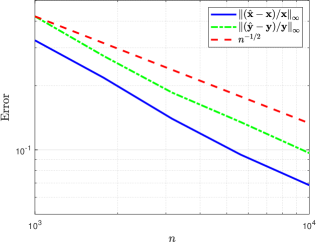
(a)

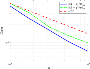
(b)

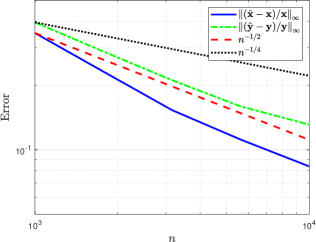
(c)

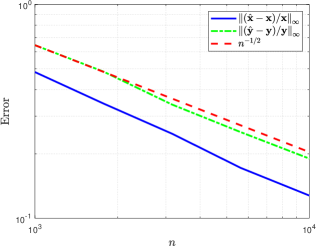
(d)

Figure 3: Maximal relative errors between $\hat{\mathbf{x}}$ and $\mathbf{x}$ and between $\hat{\mathbf{y}}$ and $\mathbf{y}$, as functions of $n$ in four different scenarios, where $S=\mathbf{x}\mathbf{y}^{T}$.

2.3 Variance matrices $S$ with arbitrary rank

In the previous section, we established that if $S=\mathbf{x}\mathbf{y}^{T}$, then $\mathbf{x}$ and $\mathbf{y}$ can be estimated accurately from $Y$ if its dimensions are sufficiently large and under mild delocalization conditions on the singular vectors of the signal $X$, even if the signal’s magnitude is arbitrarily large. In this section, we alleviate the rank-one assumption on $S$ and consider more general variance matrices.

We begin with the following definition of a doubly regular matrix.

Definition 10.

A matrix $A\in\mathbb{R}^{m\times n}$ is called doubly regular if its average entry in each row and in each column is precisely one, i.e.,

$$\frac{1}{n}A\mathbf{1}_{m}=\mathbf{1}_{n},\qquad\frac{1}{m}A^{T}\mathbf{1}_{n}=\mathbf{1}_{m}.$$ (27)

A fundamental fact crucial to our approach is that any positive matrix can be made doubly regular by appropriate scaling of its rows and columns. Specifically, since the variance matrix $S$ is positive (see (1) and the subsequent text), we have the following proposition, which is an immediate consequence of [52].

Proposition 11.

There exist positive vectors $\mathbf{x}\in\mathbb{R}^{m}$ and $\mathbf{y}\in\mathbb{R}^{n}$ such that

$$S=D\{\mathbf{x}\}\widetilde{S}D\{\mathbf{y}\},$$ (28)

where $\widetilde{S}\in\mathbb{R}^{m\times n}$ is a positive and doubly regular matrix. Moreover, the pair $(\mathbf{x},\mathbf{y})$ is unique up to the trivial scalar ambiguity, i.e., it can only be replaced with $(\alpha\mathbf{x},\alpha^{-1}\mathbf{y})$ for any $\alpha>0$.

We shall refer to $\mathbf{x}$ and $\mathbf{y}$ as the scaling factors of $S$. See [31] and the references therein for an extensive review of the topic of matrix scaling. Note that the case of $S=\mathbf{x}\mathbf{y}^{T}$, which was investigated in Section 2.2, is a special case of (28) where $\widetilde{S}$ is a matrix of ones, i.e., $\widetilde{S}=\mathbf{1}_{m\times n}$. In this case, the normalization (2) makes all of the noise variances in the matrix identical. More generally, we cannot make all noise variances identical but we can stabilize the noise variances simultaneously across rows and columns by making the noise variance matrix $(\mathbb{E}[\widetilde{E}_{ij}^{2}])=\widetilde{S}$ doubly regular. Hence, after the normalization (2), the average noise variance in each row and in each column is precisely $1$. As we shall see in Section 3, this normalization is particularly advantageous for signal detection and recovery under general heteroskedastic noise. In the remainder of this section, we investigate which structures of $S$ allow us to accurately estimate the scaling factors $\mathbf{x}$ and $\mathbf{y}$ of $S$ using $\hat{\mathbf{x}}$ and $\hat{\mathbf{y}}$ from (17). Our main result is Theorem 14 at the end of this section, which extends Theorem 9 by supporting a broader class of variance matrices $S$ with general rank, including full rank.

We begin with several definitions. Let $\mathbf{h}\in\mathbb{R}^{(m+n)}$ be the positive vector that solves (9) when replacing $S$ with $\mathbf{x}\mathbf{y}^{T}$. In particular, $\mathbf{h}^{(1)}=[\mathbf{h}_{1},\ldots,\mathbf{h}_{m}]^{T}$ and $\mathbf{h}^{(2)}=[\mathbf{h}_{m+1},\ldots,\mathbf{h}_{m+n}]^{T}$ satisfy

$$\eta+\mathbf{x}\mathbf{y}^{T}\mathbf{h}^{(2)}=\frac{1}{\mathbf{h}^{(1)}},\qquad\qquad\eta+\mathbf{y}\mathbf{x}^{T}\mathbf{h}^{(1)}=\frac{1}{\mathbf{h}^{(2)}},$$ (29)

where $\mathbf{x}$ and $\mathbf{y}$ are the scaling factors of $S$ from (28). Note that $\mathbf{h}$ depends only on $\mathbf{x}$ and $\mathbf{y}$, whereas $\mathbf{g}$ from (9) may additionally depend on $\widetilde{S}$. Next, analogously to (12), we settle the scalar ambiguity in the definition of $\mathbf{x}$ and $\mathbf{y}$ by requiring (without loss of generality) that

$$\mathbf{x}^{T}\mathbf{h}^{(1)}=\mathbf{y}^{T}\mathbf{h}^{(2)}.$$ (30)

Note that $\mathbf{g}=\mathbf{h}$ if $S=\mathbf{x}\mathbf{y}^{T}$. Therefore, Proposition 2 implies that

$$\mathbf{x}=\frac{1}{\sqrt{m-\eta\|\mathbf{h}^{(1)}\|_{1}}}\left(\frac{1}{\mathbf{h}^{(1)}}-\eta\right),\qquad\mathbf{y}=\frac{1}{\sqrt{n-\eta\|\mathbf{h}^{(2)}\|_{1}}}\left(\frac{1}{\mathbf{h}^{(2)}}-\eta\right).$$ (31)

In the previous section, we established that $\mathbf{g}$ can be estimated accurately from the data matrix $Y$ using $\hat{\mathbf{g}}$ from (15). Importantly, the estimation accuracy of $\mathbf{g}$ does not depend on the structure of the noise variance matrix $S$ (see Theorem 6 and Corollaries 7 and 8, which do not rely on Assumption 1). Hence, in cases where $\mathbf{g}$ is close to $\mathbf{h}$, it is natural to employ the formulas in (17) to estimate $\mathbf{x}$ and $\mathbf{y}$. Consequently, our primary focus in this section is to bound the discrepancy $\|\mathbf{g}-\mathbf{h}\|_{\infty}$ and describe how this discrepancy controls the accuracy of recovering $\mathbf{x}$ and $\mathbf{y}$. As we shall see, even though the estimators $\hat{\mathbf{x}}$ and $\hat{\mathbf{y}}$ in (17) were derived in the case where ${S}$ is of rank one, they can be used to accurately estimate the scaling factors $\mathbf{x}$ and $\mathbf{y}$ of $S$ in many other cases.

Let us define the positive vectors $\mathbf{w}^{(1)}\in\mathbb{R}^{m}$ and $\mathbf{w}^{(2)}\in\mathbb{R}^{n}$ according to

$$\mathbf{w}^{(1)}=D\{\mathbf{x}\}\mathbf{h}^{(1)}=\frac{\mathbf{x}}{\eta+a\mathbf{x}},\qquad\mathbf{w}^{(2)}=D\{\mathbf{y}\}\mathbf{h}^{(2)}=\frac{\mathbf{y}}{\eta+a\mathbf{y}},$$ (32)

where $a=\mathbf{x}^{T}\mathbf{h}^{(1)}=\mathbf{y}^{T}\mathbf{h}^{(2)}$; see (29) and (30). Note that $\mathbf{w}^{(1)}$ and $\mathbf{w}^{(2)}$ depend only on $\mathbf{x}$ and $\mathbf{y}$ and not on $\widetilde{S}$. To further clarify the correspondence between the pairs $(\mathbf{x},\mathbf{y})$ and $(\mathbf{w}^{(1)},\mathbf{w}^{(2)})$, we have the following proposition, whose proof can be found in Appendix K.

Proposition 12.

The sign of $\mathbf{w}_{i}^{(1)}-\mathbf{w}_{j}^{(1)}$ ($\mathbf{w}_{i}^{(2)}-\mathbf{w}_{j}^{(2)}$) is identical to the sign of $\mathbf{x}_{i}-\mathbf{x}_{j}$ ($\mathbf{y}_{i}-\mathbf{y}_{j}$), and

$$\left|\frac{\mathbf{w}_{i}^{(1)}-\mathbf{w}_{j}^{(1)}}{\mathbf{w}_{j}^{(1)}}\right|\leq\left|\frac{\mathbf{x}_{i}-\mathbf{x}_{j}}{\mathbf{x}_{j}}\right|,\qquad\left|\frac{\mathbf{w}_{i}^{(2)}-\mathbf{w}_{j}^{(2)}}{\mathbf{w}_{j}^{(2)}}\right|\leq\left|\frac{\mathbf{y}_{i}-\mathbf{y}_{j}}{\mathbf{y}_{j}}\right|,$$ (33)

for all $i\in[m]$ and $j\in[n]$. Moreover, equality holds in the two inequalities above only if $x_{i}=x_{j}$ and $y_{i}=y_{j}$, respectively.

Proposition 12 shows that the entries of $\mathbf{w}^{(1)}$ ($\mathbf{w}^{(2)}$) preserve the same ranking as the entries of $\mathbf{x}$ ($\mathbf{y}$). Moreover, the pairwise relative differences between the entries of $\mathbf{w}^{(1)}$ ($\mathbf{w}^{(2)}$) are always smaller or equal to the corresponding relative pairwise differences between the entries of $\mathbf{x}$ ($\mathbf{y}$). In this sense, the entries of $\mathbf{w}^{(1)}$ and $\mathbf{w}^{(2)}$ are always closer to being constant than the entries of $\mathbf{x}$ and $\mathbf{y}$, respectively.

We now have the following lemma, which bounds the discrepancy between $\mathbf{g}$ and $\mathbf{h}$ in terms of $\widetilde{S}$ and the vectors $\mathbf{w}^{(1)}$ and $\mathbf{w}^{(2)}$, where $\langle\cdot\rangle$ denotes the average entry in a vector.

Lemma 13.

Under Assumptions 2 and 5, there exists a constant $C^{{}^{\prime}}>0$ such that

$$\|\mathbf{g}-\mathbf{h}\|_{\infty}\leq C^{{}^{\prime}}\max\left\{\frac{1}{\sqrt{n}}\left\|\left(\widetilde{S}-1\right)\frac{\mathbf{w}^{(2)}-\langle\mathbf{w}^{(2)}\rangle}{\|\mathbf{w}^{(2)}\|_{2}}\right\|_{\infty},\frac{\sqrt{m}}{n}\left\|\left(\widetilde{S}-1\right)^{T}\frac{\mathbf{w}^{(1)}-\langle\mathbf{w}^{(1)}\rangle}{\|\mathbf{w}^{(1)}\|_{2}}\right\|_{\infty}\right\}.$$ (34)

The proof of Lemma 13 is found in Appendix J and relies on a stability analysis of the Dyson equation on the imaginary axis, which may be of independent interest; see Lemma 20 in Appendix C.4. First, Lemma 13 shows that the error $\|\mathbf{g}-\mathbf{h}\|_{\infty}$ is small if $\widetilde{S}$ is sufficiently close to the matrix of all ones $\mathbf{1}_{m\times n}$, or alternatively, if $\mathbf{w}^{(1)}$ and $\mathbf{w}^{(2)}$ are sufficiently close to being constant vectors (i.e., vectors whose entries are nearly identical). In particular, if $\mathbf{x}$ and $\mathbf{y}$ are multiples of the all-ones vectors $\mathbf{1}_{m}$ and $\mathbf{1}_{n}$, respectively, then according to Proposition 12, $\mathbf{w}^{(1)}$ and $\mathbf{w}^{(1)}$ are also multiples of the all-ones vectors $\mathbf{1}_{m}$ and $\mathbf{1}_{n}$, in which case we have $\mathbf{g}=\mathbf{h}$ by Lemma 13. In other words, we have $\mathbf{g}=\mathbf{h}$ whenever $S$ is a scalar multiple of a doubly regular matrix, regardless of its rank. Second, Lemma 13 shows that the error $\|\mathbf{g}-\mathbf{h}\|_{\infty}$ is small if $\mathbf{w}^{(1)}$ and $\mathbf{w}^{(2)}$ are sufficiently incoherent with respect to $(\widetilde{S}-1)$. Below we provide two examples demonstrating this scenario using random priors imposed on $\widetilde{S}$.

Example 1.

Consider a matrix $\widetilde{S}$ given by

$$\widetilde{S}_{ij}=1+z_{ij}-\frac{1}{m}\sum_{i=1}^{m}z_{ij}-\frac{1}{n}\sum_{j=1}^{n}z_{ij}+\frac{1}{mn}\sum_{i=1}^{m}\sum_{j=1}^{n}z_{ij},$$ (35)

where $\{z_{ij}\}\in[a-1,b-1]$ are independent random variables with zero mean and $b>1>a>0$ are fixed constants. By construction, $\widetilde{S}$ is always doubly regular and is also positive with high probability for all sufficiently large $m$ and $n$. Importantly, if $\mathbf{x}$ and $\mathbf{y}$ are either deterministic or random but generated independently of $\{z_{ij}\}$, then by standard concentration arguments [24] together with the union bound, we have

$$\frac{1}{\sqrt{n}}\left\|\left(\widetilde{S}-1\right)\frac{\mathbf{w}^{(2)}-\langle\mathbf{w}^{(2)}\rangle}{\|\mathbf{w}^{(2)}\|_{2}}\right\|_{\infty} \leq C^{{}^{\prime\prime}}\frac{\left\|\mathbf{w}^{(2)}-\langle\mathbf{w}^{(2)}\rangle\right\|_{2}}{\|\mathbf{w}^{(2)}\|_{2}}\sqrt{\frac{{\log n}}{{n}}}\leq C^{{}^{\prime\prime}}\sqrt{\frac{{\log n}}{{n}}},$$ (36)

$$\frac{\sqrt{m}}{n}\left\|\left(\widetilde{S}-1\right)^{T}\frac{\mathbf{w}^{(1)}-\langle\mathbf{w}^{(1)}\rangle}{\|\mathbf{w}^{(1)}\|_{2}}\right\|_{\infty} \leq C^{{}^{\prime\prime}}\frac{\left\|\mathbf{w}^{(1)}-\langle\mathbf{w}^{(1)}\rangle\right\|_{2}}{\|\mathbf{w}^{(1)}\|_{2}}\sqrt{\frac{\log n}{n}}\leq C^{{}^{\prime\prime}}\sqrt{\frac{{\log n}}{{n}}},$$ (37)

with probability that approaches $1$ as $m,n\rightarrow\infty$, where $C^{{}^{\prime\prime}}>0$ is a global constant. Here, we also used the fact that $m\leq n$, $\left\|\mathbf{w}^{(2)}-\langle\mathbf{w}^{(2)}\rangle\right\|_{2}\leq\left\|\mathbf{w}^{(2)}\right\|_{2}$, and $\left\|\mathbf{w}^{(1)}-\langle\mathbf{w}^{(1)}\rangle\right\|_{2}\leq\left\|\mathbf{w}^{(1)}\right\|_{2}$. We see that in this case, the upper bound in (34) is of the order of $\sqrt{\log n/n}$ with high probability, regardless of $\mathbf{w}^{(1)}$ and $\mathbf{w}^{(2)}$. If, in addition, the entries of $\mathbf{w}^{(1)}$ and $\mathbf{w}^{(2)}$ are approximately constant, then the quantities ${\left\|\mathbf{w}^{(2)}-\langle\mathbf{w}^{(2)}\rangle\right\|_{2}}/{\|\mathbf{w}^{(2)}\|_{2}}$ and ${\left\|\mathbf{w}^{(1)}-\langle\mathbf{w}^{(1)}\rangle\right\|_{2}}/{\|\mathbf{w}^{(1)}\|_{2}}$ will be small and the the upper bound in (34) will further improve. According to Proposition 12, the entries of $\mathbf{w}^{(1)}$ and $\mathbf{w}^{(2)}$ are approximately constant if the entries of $\mathbf{x}$ and $\mathbf{y}$ are approximately constant, respectively.

Example 2.

Consider a matrix $\widetilde{S}$ given by

$$\widetilde{S}=1+\sum_{k=1}^{\rho-1}\left(\nu_{k}-\langle\nu_{k}\rangle\right)\left(\xi_{k}-\langle\xi_{k}\rangle\right)^{T},$$ (38)

where $\{\nu_{k}\}_{k=1}^{\rho-1}\in\mathbb{R}^{m}$ and $\{\xi_{k}\}_{k=1}^{\rho-1}\in\mathbb{R}^{n}$ are random vectors whose entries are independent, have zero mean, and are bounded such that $\sum_{k}(\nu_{k}\xi_{k}^{T})_{ij}\in[a-1,b-1]$ for all $i\in[m]$ and $j\in[n]$ for some fixed constants $b>1>a>0$ and $\rho\in\{1,\ldots,m\}$. As in Example 1, $\widetilde{S}$ is doubly regular by construction and is positive with high probability for sufficiently large $m$ and $n$. In this case, if $\mathbf{x}$ and $\mathbf{y}$ are either deterministic or random but generated independently of $\{\nu_{k}\}$ and $\{\xi_{k}\}$, then by the same concentration arguments used in Example 1, the bounds (36) and (37) also hold here (with probability approaching $1$ as $m,n\rightarrow\infty$). The main difference here from Example 1 is that $\widetilde{S}$ is constructed to be low-rank and its entries are highly dependent, whereas in Example 1, the variables $\{z_{ij}\}$ are independent and the resulting $\widetilde{S}$ is full-rank with probability one.

Examples 1 and 2 show that the error $\|\mathbf{g}-\mathbf{h}\|_{\infty}$ is small for a wide range of noise variance matrices $S=D\{\mathbf{x}\}\widetilde{S}D\{\mathbf{y}\}$ where $\widetilde{S}$ is sufficiently generic and incoherent with respect to $\mathbf{x}$ and $\mathbf{y}$. Moreover, in these cases, the bound on the error $\|\mathbf{g}-\mathbf{h}\|_{\infty}$ is further reduced if $\mathbf{w}^{(1)}$ and $\mathbf{w}^{(2)}$ are close to being constant vectors, which is determined directly by the variability of the entries of $\mathbf{x}$ and $\mathbf{y}$ according to Proposition 12.

In cases where $\mathbf{g}$ is close to $\mathbf{h}$, we expect the formulas in (17) to provide accurate estimates of $\mathbf{x}$ and $\mathbf{y}$. To guarantee the convergence of $\hat{\mathbf{x}}$ and $\hat{\mathbf{y}}$ from (17) to $\mathbf{x}$ and $\mathbf{y}$, respectively, and provide corresponding rates, it is convenient to make the assumption that $\mathbf{g}$ approaches $\mathbf{h}$ at least with some fractional power of $n$. Specifically, we assume that

Assumption 7.

There exist constants $\widetilde{C}_{3},\delta_{3}>0$ such that $\|\mathbf{g}-\mathbf{h}\|_{\infty}\leq\widetilde{C}_{3}n^{-\delta_{3}}$.

For instance, if $m$ and $n$ are sufficiently large and the noise variance matrix $S$ is generated according to Example 1 or Example 2, then Assumption 7 is satisfied with high probability using, e.g., $\delta_{3}=0.49$. Aside from these constructions, Assumption 7 allows for more general classes of variance matrices $S$ where $\delta_{3}$ can be an arbitrarily small positive constant.

To state our main result in this section, which extends Theorem 9, we replace Assumption 6 from Section 2.2 with the following assumption, which similarly requires that $m$ grows sufficiently quickly with $n$.

Assumption 8.

There exist constants $\widetilde{C}_{4},\delta_{4}>0$ such that $m\geq\widetilde{C}_{4}\max\{n^{1/2+\delta_{4}},n^{1-\delta+\delta_{4}},n^{1-\delta_{3}+\delta_{4}}\}$.

Recall that $\delta>0$ is from Assumption 4, which controls the delocalization level of the singular vectors of the signal $X$. Similarly to Assumption 6 in the previous section, Assumption 8 always holds if $m$ is proportional to $n$ (since one can take any $\delta_{4}<\min\{\delta,\delta_{3},0.5\}$). Now, we can extend Theorem 9 to cover general variance matrices $S$ as long as $\mathbf{g}$ is close to $\mathbf{h}$ for large $m$ and $n$.

Theorem 14.

Under Assumptions 2,3,4,5,7, for any $\epsilon>0$ there exist $C^{{}^{\prime}},c^{{}^{\prime}}(t)>0$ such that

$$\left\|\frac{\hat{\mathbf{x}}-\mathbf{x}}{\mathbf{x}}\right\|_{\infty}\leq C^{{}^{\prime}}\max\left\{n^{\epsilon-1/2},n^{-\delta},n^{-\delta_{3}}\right\},$$ (39)

with probability at least $1-c^{{}^{\prime}}(t)n^{-t}$, for all $t>0$. Furthermore, if Assumption 8 holds, then for any $\epsilon<\delta_{4}$,

$$\left\|\frac{\hat{\mathbf{y}}-\mathbf{y}}{\mathbf{y}}\right\|_{\infty}\leq C^{{}^{\prime}}\max\left\{\frac{n^{\epsilon+1/2}}{m},\frac{n^{1-\delta}}{m},\frac{n^{1-\delta_{3}}}{m}\right\},$$ (40)

with probability at least $1-c^{{}^{\prime}}(t)n^{-t}$, for all $t>0$.

The proof of Theorem 14 is an immediate extension of the proof of Theorem 9 under Assumptions 7 and 8; see Appendix L. Theorem 14 is identical to Theorem 9 except that the bounds here depend additionally on $\delta_{3}$, which controls the closeness of $\mathbf{g}$ and $\mathbf{h}$. Intuitively, the bound on the estimation accuracy improves if the solution $\mathbf{g}$ of the true Dyson equation (10) is close to the solution $\mathbf{h}$ of the rank-one Dyson equation (29). According to Lemma 13 and Proposition 12, $\mathbf{g}$ and $\mathbf{h}$ are close if $\widetilde{S}$ is sufficiently incoherent with respect to $\mathbf{x}$ and $\mathbf{y}$, or if the entries of $\mathbf{x}$ and $\mathbf{y}$ are approximately constant (i.e., $\mathbf{x}$ and $\mathbf{y}$ are close to multiples of the all-ones vector). As noted after Assumption 7, if ${S}$ is generated as described in Examples 1 or 2 for sufficiently large $m$ and $n$, then Assumption 7 holds with high probability for $\delta_{3}=0.49$. In this case, the bounds in Theorem 14 imply almost the same rates as in Theorem 9.

In Figure 4, we illustrate the relative errors in the left-hand sides of (39) and (40) for the same experimental setup used for Figure 3, except that the variance matrix is $S=D\{\mathbf{x}\}\widetilde{S}D\{\mathbf{y}\}$, where $\widetilde{S}$ was generated according to Example 1. Specifically, $\{z_{ij}\}$ are i.i.d and sampled from $5(\operatorname{Bernoulli}(0.1)-0.1)$, i.e., $z_{ij}$ takes the value of $-0.5$ with probability $0.9$ and the value of $4.5$ with probability $0.1$. In this case, as mentioned previously, Assumption 7 is satisfied with high probability with $\delta_{3}\sim 0.5$ for sufficiently large $m$ and $n$. Therefore, according to Theorem 14, we expect the convergence rates to be the same as for the corresponding rates from Figure 3. Indeed, we observe from Figure 4 that in this case, the empirical error rates conform to the same bounds from Figure 3.

(a)

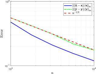
(b)

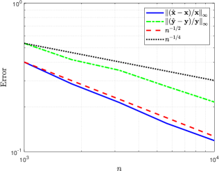
(c)

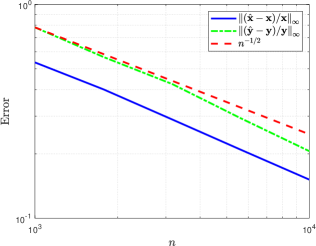
(d)

Figure 4: Maximal relative errors between $\hat{\mathbf{x}}$ and $\mathbf{x}$ and between $\hat{\mathbf{y}}$ and $\mathbf{y}$, as functions of $n$ in four different scenarios. The variance matrix here is given by $S=D\{\mathbf{x}\}\widetilde{S}D\{\mathbf{y}\}$, where $\widetilde{S}$ was generated according to Example 1.

3 Application to signal detection and recovery

3.1 Signal identification and rank estimation

We begin by reviewing the spectral behavior of homoskedastic noise. Letting $\Sigma={E}{E}^{T}/n$, we define the Empirical Spectral Distribution (ESD) of $\Sigma$ as

$$F_{\Sigma}(\tau)=\frac{1}{m}\sum_{i=1}^{m}\mathbbm{1}\left(\lambda_{i}\{\Sigma\}\leq\tau\right),$$ (41)

where $\mathbbm{1}(\cdot)$ is the indicator function and $\lambda_{i}\{\Sigma\}$ is the $i$’th largest eigenvalue of $\Sigma$. If the noise is homoskedastic, i.e., $S=\sigma^{2}\mathbf{1}_{m\times n}$ for some $\sigma>0$, then as $m,n\rightarrow\infty$ and $m/n\rightarrow\gamma\in(0,1]$, the empirical spectral distribution $F_{\Sigma}(\tau)$ converges almost surely to the Marchenko-Pastur (MP) distribution $F_{\gamma,\sigma}(\tau)$ [43], which is the cumulative distribution function of the MP density

$$dF_{\gamma,\sigma}(\tau)=\frac{\sqrt{(\beta_{+}-\tau)(\tau-\beta_{-})}}{2\pi\sigma^{2}\gamma\tau}\mathbbm{1}\left(\beta_{-}\leq\tau\leq\beta_{+}\right),$$ (42)

where $\beta_{\pm}=\sigma^{2}(1\pm\sqrt{\gamma})^{2}$. Moreover, for many types of noise distributions [21, 62], the largest eigenvalue of $\Sigma$ converges almost surely (in the same asymptotic regime) to the upper edge of the MP density, i.e., $\lambda_{1}\{\Sigma\}\overset{a.s.}{\longrightarrow}\beta_{+}$.

If the noise variance matrix $S$ is of rank one, i.e., $S=\mathbf{x}\mathbf{y}^{T}$, then the normalization (2) makes the noise completely homoskedastic, imposing the standard spectral behavior described above on $\widetilde{\Sigma}=\widetilde{E}\widetilde{E}^{T}/n$. For more general variance matrices, the normalization (2) makes the noise variance matrix doubly regular (see Proposition 11 and Definition 10). Importantly, it was shown in [39] (see Proposition 4.1 therein), that under mild regularity conditions, this normalization is sufficient to enforce the standard spectral of homoskedastic noise. Hence, we propose to use our estimates of $\mathbf{x}$ and $\mathbf{y}$ (described and analyzed in Section 2) to normalize the rows and columns of the data, thereby making the noise variance matrix close to doubly regular. Specifically, we define $\hat{Y}\in\mathbb{R}^{m\times n}$, $\hat{X}\in\mathbb{R}^{m\times n}$, and $\hat{E}\in\mathbb{R}^{m\times n}$ according to

$$\hat{Y}=(D\{\mathbf{\hat{x}}\})^{-1/2}Y(D\{\mathbf{\hat{y}}\})^{-1/2}=\hat{X}+\hat{E},$$ (43)

where $\hat{X}=(D\{\mathbf{\hat{x}}\})^{-1/2}X(D\{\mathbf{\hat{y}}\})^{-1/2}$ and $\hat{E}=(D\{\mathbf{\hat{x}}\})^{-1/2}E(D\{\mathbf{\hat{y}}\})^{-1/2}$. We now have the following theorem.

Theorem 15.

Suppose that the assumptions of Theorem 14 hold and consider the asymptotic regime $m,n\rightarrow\infty$ with $m/n\rightarrow\gamma\in(0,1]$. Then, the empirical spectral distribution of $\hat{\Sigma}=\hat{E}\hat{E}^{T}/n$, given by $F_{\hat{\Sigma}}(\tau)$ (see (41)), converges almost surely to the Marchenko-Pastur distribution with parameter $\gamma$ and variance $1$, i.e., $F_{\gamma,1}(\tau)$, for all $\tau\in\mathbb{R}$. Moreover, the largest eigenvalue of $\hat{\Sigma}$ converges almost surely to the upper edge of the MP density $\beta_{+}=(1+\sqrt{\gamma})^{2}$.

The proof of Theorem 15 can be found in Appendix M and follows closely to proof of Theorem 2.6 in [39]. Theorem 15 establishes that under suitable conditions, $\hat{E}$ enjoys the same asymptotic spectral behavior described above for homoskedastic noise, namely the same limiting spectral distribution and the limit of the largest eigenvalue. This fact allows for a simple procedure for rank estimation. If no signal is present, i.e., if $X$ is the zero matrix, then the largest eigenvalue of $\hat{Y}\hat{Y}^{T}/n$ should be close to $(1+\sqrt{m/n})^{2}$ for sufficiently large $m$ and $n$. Alternatively, if an eigenvalue of $\hat{Y}\hat{Y}^{T}/n$ exceeds the threshold $(1+\sqrt{m/n})^{2}$ by a small positive constant for sufficiently large $m$ and $n$, then we can deduce that a signal is present in the data. Moreover, since the rank of $\hat{X}$ is identical to the rank of ${X}$ (as they differ by a positive diagonal scaling), we can estimate the rank of $X$ by counting how many eigenvalues of $\hat{Y}\hat{Y}^{T}/n$ exceed $(1+\sqrt{m/n})^{2}$ by a small positive constant $\varepsilon$, i.e.,

$$\hat{r}_{\varepsilon}=\left|\left\{i\in[m]:\;\lambda_{i}\{\frac{1}{n}\hat{Y}\hat{Y}^{T}\}>\left(1+\sqrt{\frac{m}{n}}\right)^{2}+\varepsilon\right\}\right|.$$ (44)

Here, $\varepsilon$ accounts for finite-sample fluctuations of the largest eigenvalue of $\hat{E}\hat{E}^{T}/n$, which diminish as $m,n\rightarrow\infty$. It can be shown that for any fixed $\varepsilon>0$, under the conditions in Theorem 14, the rank estimator $\hat{r}_{\varepsilon}$ provides a consistent lower bound on the true rank $r$ as $n\rightarrow\infty$, namely

$$\operatorname{Pr}\{r<\hat{r}_{\varepsilon}\}\underset{n\rightarrow\infty}{\longrightarrow}0,$$ (45)

see Theorem 2.3 in [39] and its proof, which we do not repeat here for the sake of brevity. In other words, all signal components that are detected in this way are true signal components asymptotically. In what follows, we take $\varepsilon\rightarrow 0$ for simplicity and denote $\hat{r}=\hat{r}_{0}$. Algorithm 2 summarizes our proposed rank estimation procedure, noting that comparing the eigenvalues of $\hat{Y}\hat{Y}^{T}/n$ to $\beta_{+}$ is equivalent to comparing the singular values of $\hat{Y}$ to $\sqrt{m}+\sqrt{n}$.

Algorithm 2 Rank estimation

1:Input: Data matrix $Y\in\mathbb{R}^{m\times n}$ with $m\leq n$ and no rows or columns that are entirely zero.

2:Apply Algorithm 1 to obtain $\hat{Y}$.

3:Compute $\hat{r}$ by counting the number of singular values of $\hat{Y}$ that exceed $\sqrt{m}+\sqrt{n}$.

An important advantage of our proposed rank estimation technique is that the normalization of the rows and columns can enhance the spectral signal-to-noise ratio, namely, improve the ratios between the singular values of the signal and the operator norm of the noise. Specifically, it was shown in [42] (see Proposition 6.3 therein) that in the case of $E_{ij}\sim\mathcal{N}(0,S_{ij})$, $S=\mathbf{x}\mathbf{y}^{T}$, and if the singular vectors of $X$ satisfy certain genericity and weighted orthogonality conditions (see [42] for more details), then

$$\frac{\sigma_{i}^{2}\{\widetilde{X}\}}{\|\widetilde{E}\|_{2}^{2}}\geq\tau\frac{\sigma_{i}^{2}\{{X}\}}{\|{E}\|_{2}^{2}},$$ (46)

almost surely as $m,n\rightarrow\infty$ with $m/n\rightarrow\gamma$, for all $i=1,\ldots,r$, where $\sigma_{i}\{\cdot\}$ denotes the $i$’th largest singular value of a matrix and

$$\tau=\left(\frac{1}{m}\sum_{i=1}^{m}\mathbf{x}_{i}\right)\left(\frac{1}{m}\sum_{i=1}^{m}\frac{1}{\mathbf{x}_{i}}\right)\left(\frac{1}{n}\sum_{j=1}^{n}\mathbf{y}_{j}\right)\left(\frac{1}{n}\sum_{j=1}^{n}\frac{1}{\mathbf{y}_{j}}\right).$$ (47)

Here, we always have $\tau\geq 1$, where $\tau=1$ if and only if $\mathbf{x}$ and $\mathbf{y}$ are constant vectors (i.e., vectors with identical entries); see [42]. In this setting, if the noise variances are not identical across rows and/or columns, the normalization (2) will improve the signal-to-noise ratio for each signal component. Moreover, the improvement increases with the level of heteroskedasticity, i.e., with the amount of variability of the entries in $\mathbf{x}$ and $\mathbf{y}$ as encoded by $\tau$. Importantly, even if some of the signal components are originally below the spectral noise level, i.e., ${\sigma_{i}\{{X}\}}<{\|{E}\|_{2}}$, the corresponding signal components after the normalization (2) can exceed it if $\tau$ is sufficiently large. Under the conditions in Theorem 9 in Section 2.2, which allow us to estimate $\mathbf{x}$ and $\mathbf{y}$ accurately for large matrix dimensions, our proposed normalization (43) will enhance the spectral signal-to-noise ratio analogously.

More generally, the normalization (2) can significantly reduce the operator norm of the noise with respect to the average noise variance in the data. This advantage holds for general noise distributions and variance patterns regardless of the signal. To explain this advantage, suppose for simplicity that the average noise variance across all entries in the original data is one, i.e., $\sum_{ij}S_{ij}/(mn)=1$. This property also holds after the normalization (2) since the corresponding noise variance matrix is doubly regular. On the one hand, before the normalization, we have the inequality

$$\frac{1}{n}\mathbb{E}\|{E}\|^{2}_{2}\geq\max\left\{\max_{i\in[n]}\left\{\frac{1}{n}\sum_{j=1}^{n}S_{ij}\right\},\left(\frac{m}{n}\right)\max_{j\in[m]}\left\{\frac{1}{m}\sum_{i=1}^{m}S_{ij}\right\}\right\},$$ (48)

which follows from the fact that the operator norm of a matrix is lower-bounded by the Euclidean norm of any of its rows or columns. Hence, the quantity $\mathbb{E}\|{{E}}\|^{2}_{2}/n$ will be large if the average noise variance in at least one of the rows or columns is large. For instance, if $m/n=\gamma=0.5$ and the average noise variance in one of the rows or columns is $100$, then $\mathbb{E}\|{{E}}\|^{2}_{2}/n$ must be at least $50$ (see Figure 1 in the introduction for an illustration). On the other hand, after the normalization (2), the quantity $\mathbb{E}\|\widetilde{{E}}\|^{2}_{2}/n=\mathbb{E}[\lambda_{1}\{\widetilde{E}\widetilde{E}^{T}/n\}]$ approaches the MP upper edge $(1+\sqrt{\gamma})^{2}$ in the asymptotic regime $m,n\rightarrow\infty$ with $m/n\rightarrow\gamma$. Crucially, $(1+\sqrt{\gamma})^{2}$ is upper bounded by $4$ for all $\gamma\in(0,1]$. Therefore, the operator norm of the noise can be substantially reduced by the normalization (2) while keeping the average noise variance in the data the same. This advantage holds similarly for the normalization (43) whenever $\mathbf{x}$ and $\mathbf{y}$ are accurately estimated by $\hat{\mathbf{x}}$ and $\hat{\mathbf{y}}$, respectively (see Section 2.3).

Figure 5 depicts the spectrum of a matrix $Y$ of size $1000\times 2000$ before and after the normalizations (2) and (43), where the true scaling factors $\mathbf{x}$ and $\mathbf{y}$ were computed by the Sinkhorn-Knopp algorithm [52, 53] applied to $S$. Here, the signal matrix $X$ is of rank $r=10$ with singular values $s_{1},\ldots,s_{10}=\sqrt{10n}$, where the singular vectors were drawn from random Gaussian vectors followed by orthonormalization. The noise entries $E_{ij}$ were sampled independently from $\mathcal{N}(0,S_{ij})$, where $S$ is of rank $30$ and was generated according to $S=AB$, $A\in\mathbb{R}^{m\times 30}$, $B\in\mathbb{R}^{30\times n}$, $A_{ij},B_{ij}\sim\operatorname{exp}\{\mathcal{N}(0,t^{2})\}$, and $t$ is the heteroskedasticity parameter ($t=0$ corresponds to homoskedastic noise). We then fixed $t=2$ and normalized $S$ by a scalar so that its average entry is $1$. Since the entries of $A$ and $B$ are generated from a log-normal distribution, the entries of $S$ can differ substantially across rows and columns.

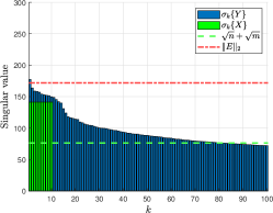
(a)

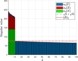
(b)

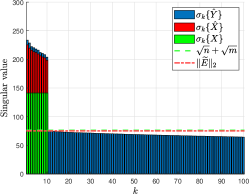
(c)

(d)

(e)

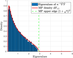
(f)

Figure 5: The spectrum of the original data matrix (panel (a)) and after applying the normalizations (2) (panel(b)) and (43), where $m=1000$, $n=2000$, and $r=10$.

Figure 5 shows that for the original data, the spectral noise level $\|E\|_{2}$ exceeds the signal singular values $\sigma_{i}\{X\}$. Moreover, the largest singular value of $Y$ corresponds to the noise level $\|{E}\|_{2}$ almost perfectly. Hence, the signal components are undetectable by traditional approaches that compare the singular values of $Y$ to the noise level. Moreover, the data singular values do not admit any noticeable gap after the $10$’th singular value, and the eigenvalue density of $YY^{T}/n$ does not fit the MP law. In particular, the eigenvalue density of $YY^{T}/n$ is much more spread out than the MP density, with a large number of eigenvalues that exceed the upper edge $\beta_{+}$. These large eigenvalues arise due to the heteroskedasticity of the noise. However, after our proposed normalizations, the signal singular values increase and the noise level decreases simultaneously, revealing the signal components and allowing for their easy detection. Specifically, we immediately see a large gap after the $10$’th singular value of $\widetilde{Y}$ and $\hat{Y}$, while the $11$’th singular values is just below the critical threshold $\sqrt{n}+\sqrt{m}$, which is very close to $\|{\widetilde{E}}\|_{2}$ and $\|{\hat{E}}\|_{2}$. Furthermore, the eigenvalue densities of $\widetilde{Y}\widetilde{Y}^{T}/n$ and $\hat{Y}\hat{Y}^{T}/n$ are very close to the MP law, even though the noise variances after the normalizations (2) and (43) are not identical (since $S$ is not rank-one).

3.2 Low-rank signal recovery

In the previous section, we showed that normalizing the rows and columns of the data matrix according to (43) can be highly beneficial for signal detection. In particular, the normalization standardizes the spectral behavior of the noise and can improve the spectral signal-to-noise ratio. In this section, we propose to leverage these advantages for improved recovery of the low-rank signal matrix $X$. Specifically, instead of applying a low-rank approximation to the original data matrix $Y$, where the noise can be highly heteroskedastic, we advocate applying a low-rank approximation to the normalized matrix $\hat{Y}$ and then un-normalize the rows and columns of the resulting matrix. We motivate and justify this approach through maximum-likelihood estimation and weighted low-rank approximation. We then demonstrate the practical advantages of this approach in simulations.

Let us consider the case of Gaussian heteroskedastic noise $E_{ij}\sim\mathcal{N}(0,S_{ij})$. In this case, we have $Y_{ij}\sim\mathcal{N}(X_{ij},S_{ij})$, where we treat $X$ as a deterministic parameter to be estimated. The negative log-likelihood of observing $Y$ is given by

$$\mathcal{L}_{S}(X)=\frac{1}{2}\sum_{i=1}^{m}\sum_{j=1}^{n}\left[\frac{|X_{ij}-Y_{ij}|^{2}}{S_{ij}}+\log(2\pi S_{ij})\right].$$ (49)

If the signal’s rank $r$ is known, then the maximum-likelihood estimate of $X$ is obtained by minimizing $\mathcal{L}_{S}(\Theta)$ over all matrices $\Theta\in\mathbb{R}^{m\times n}$ of rank $r$. This is equivalent to minimizing

$$\widetilde{\mathcal{L}}_{S}(\Theta)=\sum_{i=1}^{m}\sum_{j=1}^{n}\frac{|\Theta_{ij}-Y_{ij}|^{2}}{S_{ij}},$$ (50)

over all rank-$r$ matrices, a problem known as weighted low-rank approximation [54]. Specifically, the goal is to find an $m\times n$ matrix of rank $r$ that best fits the data $Y$ in a weighted least-squares sense, where the weights are inversely proportional to the noise variances in the data.

If the noise variance matrix $S$ is of rank one, i.e., $S=\mathbf{x}\mathbf{y}^{T}$, then the weighted low-rank approximation problem admits a simple closed-form solution that can be written via the normalization (2). Specifically, the minimizer of $\widetilde{\mathcal{L}}_{\mathbf{x}\mathbf{y}^{T}}(\Theta)$ over all matrices $\Theta$ of rank $r$ is given by (see, e.g., [32, 54])

$$(D\{\mathbf{x}\})^{1/2}T_{r}\{\widetilde{Y}\}(D\{\mathbf{y}\})^{1/2},$$ (51)

where $\widetilde{Y}$ is from (2) and $T_{r}\{\widetilde{Y}\}$ is the closest rank-$r$ matrix to $\widetilde{Y}$ in Frobenius norm. In other words, if $S=\mathbf{x}\mathbf{y}^{T}$, then the solution to the weighted low-rank approximation problem is given by first scaling the rows and columns of the data matrix $Y$ according to (2), then truncating the SVD of the normalized matrix to its $r$ largest components, and lastly, unscaling the rows and columns of the resulting rank-$r$ matrix. Since $\mathbf{x}$ and $\mathbf{y}$ are unknown, we replace them with their estimates $\hat{\mathbf{x}}$ and $\hat{\mathbf{y}}$ from Algorithm 1. Further, we replace the true rank $r$ with its estimate $\hat{r}$ from Section 3.1 (see Algorithm 2). Overall, we obtain the signal estimate

$$\overline{X}=(D\{\hat{\mathbf{x}}\})^{1/2}T_{\hat{r}}\{\hat{{Y}}\}(D\{\hat{\mathbf{y}}\})^{1/2}.$$ (52)

If the variance matrix $S$ is not rank-one, then the weighted low-rank approximation problem does not admit a closed-form solution [54]. Since it is a non-convex optimization problem, solving it can be highly prohibitive from a computational perspective, particularly for large matrix dimensions. Therefore, it is advantageous to replace the variance matrix $S$ in the weighted low-rank approximation problem with a rank-one surrogate. As we show below, replacing $S$ in $\mathcal{L}_{S}$ from (49) with $\mathbf{x}\mathbf{y}^{T}$, where $\mathbf{x}$ and $\mathbf{y}$ are the scaling factors of $S$ from Proposition 11, has a favorable interpretation from the viewpoint of approximate maximum-likelihood estimation in the Gaussian noise model. Specifically, we have the following proposition, whose proof can be found in Appendix N.

Proposition 16.

For any fixed signal $X$, the matrix $\mathbf{x}\mathbf{y}^{T}$ is the unique minimizer of $\mathbb{E}[\mathcal{L}_{A}(X)]$ over all positive matrices $A\in\mathbb{R}^{m\times n}$ of rank one, where $\mathbf{x}$ and $\mathbf{y}$ are from Proposition 11 and the expectation is over $\{Y_{ij}\sim\mathcal{N}(X_{ij},S_{ij})\}$. If we alleviate the rank-one requirement, then the corresponding minimizer is $S$.

In other words, among all positive rank-one matrices $A$ that act as surrogates for $S$, taking $A=\mathbf{x}\mathbf{y}^{T}$ in $\mathcal{L}_{A}(X)$ provides the best approximation, on average, to the true negative log-likelihood $\mathcal{L}_{S}(X)$ of observing the data in the Gaussian noise model. Hence, if we want to replace $S$ with a rank-one surrogate for approximate maximum-likelihood estimation, i.e., when minimizing $\mathcal{L}_{A}(\Theta)$ over all rank-$r$ matrices, it is natural to use $A=\mathbf{x}\mathbf{y}^{T}$. Note that $\mathbf{x}\mathbf{y}^{T}$ is generally not the best rank-one approximation to $S$ in Frobenius norm.

As explained above, in the Gaussian noise model, the weighted low-rank approximation problem of minimizing $\widetilde{\mathcal{L}}_{\mathbf{x}\mathbf{y}^{T}}(\Theta)$ over all matrices $\Theta$ of rank $r$ is a natural surrogate for the true maximum-likelihood estimation problem when $S$ is not rank-one. More broadly, the rationale for solving this problem is to penalize noisy rows and columns in the data while allowing for a simple closed-form solution to the weighted low-rank approximation problem. In this context, the noise levels in the rows and columns are encoded by the scaling factors $\mathbf{x}$ and $\mathbf{y}$ from Proposition 11, which can be estimated accurately by $\hat{\mathbf{x}}$ and $\hat{\mathbf{y}}$ from (17), respectively, in a broad range of settings (see Section 2.3). Consequently, even if the noise is highly heteroskedastic with a general variance pattern, it is advantageous to use (52) to estimate the low-rank signal $X$. Algorithm 3 summarizes our proposed approach for signal recovery.

Algorithm 3 Adaptively weighted low-rank approximation

1:Input: Data matrix $Y\in\mathbb{R}^{m\times n}$ with $m\leq n$ and no rows or columns that are entirely zero.

2:Apply Algorithms 1 and 2 to $Y$, obtaining $\hat{Y}$, $\hat{\mathbf{x}}$, $\hat{\mathbf{y}}$, and $\hat{r}$.

3:Compute $T_{\hat{r}}\{\hat{{Y}}\}$ by truncating the SVD of $\hat{Y}$ to its $\hat{r}$ largest components.

4:Form the estimated signal matrix $\overline{X}=(D\{\hat{\mathbf{x}}\})^{1/2}T_{\hat{r}}\{\hat{{Y}}\}(D\{\hat{\mathbf{y}}\})^{1/2}$.

The solution (51) to the weighted low-rank approximation problem with $S=\mathbf{x}\mathbf{y}^{T}$ involves the operator $T_{r}$, which truncates the SVD of the input matrix to its $r$ leading components. This operator can be replaced with a more general matrix denoising operator. For the Gaussian noise model with $S=\mathbf{x}\mathbf{y}^{T}$, [41] proposed to use $\mathcal{T}_{r}\{A\}=\sum_{i=1}^{r}\sum_{j=1}^{r}u_{i}\theta_{ij}v_{j}$, where $\{u_{i}\}$ and $\{v_{j}\}$ are the left and right singular vectors of $A$, respectively, and $\{\theta_{ij}\}$ are tunable parameters. This matrix denoising operator generalizes singular value shrinkage [19] (which manipulates the singular values of a matrix) by allowing for all possible cross-products of left and right singular vectors. [41] derived the optimally-tuned parameters $\{\theta_{ij}\}$ that minimize the weighted loss

$$\left\|\left(D\{\mathbf{x}\}\right)^{1/2}\left(\mathcal{T}_{r}\{\widetilde{Y}\}-\widetilde{X}\right)\left(D\{\mathbf{y}\}\right)^{1/2}\right\|_{F}^{2}=\left\|\left(D\{\mathbf{x}\}\right)^{1/2}\mathcal{T}_{r}\{\widetilde{Y}\}\left(D\{\mathbf{y}\}\right)^{1/2}-X\right\|_{F}^{2}$$ (53)

asymptotically as $m,n\rightarrow\infty$ and $m/n\rightarrow\gamma$ under suitable conditions. The corresponding estimator of $X$ is then given by $(D\{\mathbf{x}\})^{1/2}\mathcal{T}_{r}\{\widetilde{Y}\}(D\{\mathbf{y}\})^{1/2}$, which is analogues to (51) when replacing $T_{r}$ with $\mathcal{T}_{r}$. We refer to this approach as weighted-loss denoising (WLD). Analogously to our adaptively weighted low-rank approximation approach, we propose to replace $\mathbf{x}$ and $\mathbf{y}$ with our estimates $\hat{\mathbf{x}}$ and $\hat{\mathbf{y}}$ from (17), respectively.

In Figure 6, we demonstrate the advantages of the normalization (43) for recovering $X$ – either by truncating the SVD after our normalization (Algorithm 3) or via WLD with our estimated scaling factors $\hat{\mathbf{x}}$ and $\hat{\mathbf{y}}$. Specifically, we compare several methods for recovering $X$: 1) Oracle singular value thresholding (SVT) of $Y$, i.e., $T_{r^{{}^{\prime}}}\{Y\}$, where $r^{{}^{\prime}}$ is set to minimize the error with respect to $X$ in Frobenius norm ($X$ is provided for optimally tuning $r^{{}^{\prime}}$); b) Oracle singular value shrinkage (SVS) of $Y$, i.e., $\mathcal{T}_{r}\{Y\}$, where the parameters $\{\theta_{ij}\}$ are nonzero only for $i=j$ and are set to minimize the error with respect to $X$ in Frobenius norm ($X$ is provided for optimally tuning $\{\theta_{ii}\}$); c) WLD [42], where $\mathbf{x}$ and $\mathbf{y}$ are estimated as described in [42] from the Euclidean norms of the rows and columns of $Y$ (listed as “traditional normalization” in the legend of Figure 6); d) SVT at rank $\hat{r}$ after our proposed normalization (43), i.e., Algorithm 3; and (e) WLD [42] combined with our proposed normalization (43), namely, replacing $T_{\hat{r}}$ in (52) with $\mathcal{T}_{\hat{r}}$. In this experiment, the dimensions are $m=1000$, $n=2000$, and the noise $E$ is Gaussian heteroskedastic as described for Figure 5 (see details in Section 3.1). The signal $X$ has $r=20$ nonzero singular values equal to $s$ and the singular vectors are orthonormalized Gaussian random vectors whose support was restricted to half the rows and half the columns. Hence, the signal $X$ is localized to a quarter of the entries. We then evaluated the relative mean squared error (MSE) of the recovery for each method, i.e., the squared Frobenius norm of the difference between each method’s output and $X$, relative to $\|X\|_{F}^{2}$, followed by averaging the results over $10$ randomized experiments.

In Figure 6a, we depict the relative MSE versus the signal strength $s$ while the noise heteroskedasticity level is fixed at $t=2$ (see the details of the noise generation in Section 3.1). It is evident that our proposed normalization combined with WLD provides the best performance. Very similar performance is achieved by Algorithm 3, i.e., when truncating the singular values after our normalization, with a slight advantage to WLD for weak signals. However, when applying WLD with the traditional normalization proposed in [42], which relies on $(Y_{ij}^{2})$ to estimate $\mathbf{x}$ and $\mathbf{y}$, the performance deteriorates significantly for strong signals since the corresponding estimators for $\mathbf{x}$ and $\mathbf{y}$ become highly inaccurate. Moreover, we see that truncating or shrinking the singular values of the original data $Y$, even if optimally tuned using an oracle that provides the true signal $X$, is always suboptimal to normalizing the data. This is most notable for weak signals, e.g., $s=2\sqrt{n}$, where the difference between the relative MSEs before and after normalization is substantial.

In Figure 6b, we depict the relative MSE versus the noise heteroskedasticity level $t$ while the signal strength is fixed at $s=3\sqrt{n}$. It is evident that when no heteroskedasticity is present, i.e., $t=0$, all methods perform similarly. In this case, oracle SVS is almost identical to our normalization + WLD, while oracle SVT is almost identical to our normalization + SVT. Indeed, if the noise is homoskedastic, then no normalization should be performed, i.e., $\hat{\mathbf{x}}$ and $\hat{\mathbf{y}}$ should be close to vectors of all-ones (up to a possible global factor). Hence, we see that our normalization does not degrade the performance in this case. However, as $t$ increases, the noise becomes more heteroskedastic, and all normalization-based approaches significantly outperform SVT or SVS applied to the original data.

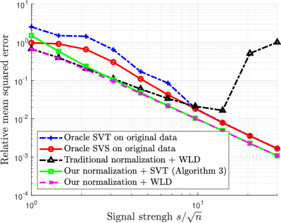
(a)

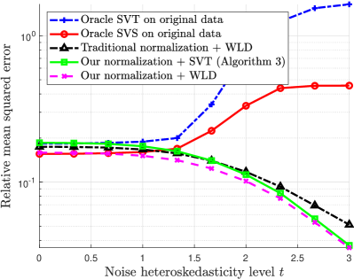
(b)

Figure 6: Comparison of the relative MSE of recovering $X$ using different methods, where $m=1000$, $n=2000$, and $r=20$. The noise here is Gaussian heteroskedastic, generated as described in Section 3.1 for Figure 5. Panel (a) depicts the relative MSE versus the signal strength $s/\sqrt{n}$ while fixing the heteroskedasticity level at $t=2$. Panel (b) depicts the relative MSE versus the heteroskedasticity level $t$ while fixing the signal strength at $s=3\sqrt{n}$.

4 Examples on real data

Next, we demonstrate the effect of our proposed normalization on the spectrum of experimental genomics data. We compare our approach to the method of [39], which assumes that the data satisfies a quadratic variance function (QVF) for estimating the scaling factors $\mathbf{x}$ and $\mathbf{y}$. In our experiments, we used data from Single-Cell RNA Sequencing (scRNA-seq) and Spatial Transcriptomics (ST). Specifically, we used the scRNA-seq dataset of purified peripheral blood mononuclear cells (PBMCs) of Zheng et al. [64] and the Visium ST dataset of human dorsolateral prefrontal cortex from Maynard et. al. [44].

We applied several preliminary preprocessing steps to the datasets to control their size and sparsity. For the scRNA-seq data, which originally contained $\sim 95000$ rows (cells) and $\sim 33000$ columns (genes), we randomly sampled $5000$ rows and then removed all rows and columns with less than $50$ nonzero entries, resulting in a matrix of size $\sim 5000\times 7500$. For the ST data, which originally contained $\sim 3600$ rows (pixels) and $\sim 33000$ genes, we did not apply any downsampling, but we applied an analogous sparsity filtering step with a threshold of $20$ nonzeros per row and column, resulting in a matrix of size $\sim 5000\times 15000$.

Figures 7a, 7b, and 7c, depict the empirical eigenvalue densities of the raw scRNA-seq data, the corresponding data after the normalization of [39] (where we used the procedure described therein to adaptively find the QVF parameters), and the data after Algorithm 1, respectively. Analogously, Figures 7d, 7e, and 7f, depict the corresponding empirical eigenvalue densities for the ST data. We mention that for visualization purposes, we normalized the raw scRNA-seq and ST data by a scalar to match the median of the eigenvalues of $YY^{T}/n$ to the median of the MP law. It is evident that the eigenvalue densities of the raw scRNA-seq and ST data are very different from the MP density and are much more spread out. On the other hand, after normalization of the rows and columns using the estimated scaling factors of either [39] or our proposed approach here, we obtain accurate fits to the MP law.

Next, we applied a sequence of two common transformations to the scRNA-seq and ST data matrices. First, we normalized each row of the data matrices so that their entries sum to $1$. This step is known as library normalization and is used to mitigate the influence of technical variability of counts (also known as “read depth”) across cell populations [59, 11]. Second, we removed the empirical mean of each column (gene), which is a common step used for principal components analysis. The resulting data matrices contain negative entries, so we cannot apply the method of [39] directly. Instead, we used the absolute values of the transformed data entries to estimate the scaling factors $\mathbf{x}$ and $\mathbf{y}$ via the method of [39]. Figures 7g, 7h, 7i, 7j, 7k, and 7l depict the empirical eigenvalue densities of the transformed data analogously to Figures 7a, 7b, 7c, 7d, 7e, and 7f. It is evident that similarly to the raw data, the eigenvalue density of the transformed data does not fit the MP law and is much more spread out. Yet, for the transformed data, the method of [39] no longer provides accurate fits to the MP law, arguably because the transformed data does not satisfy the required QVF condition. On the other hand, our proposed approach still provides excellent fits to the MP law for the transformed data of scRNA-seq and ST. The main advantage of our approach here is that it does not rely on the particular distributions of the noise entries nor their relation to the signal. Therefore, our approach can support many common transformations of the data that are useful for downstream analysis.

(a)

(b)

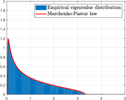
(c)

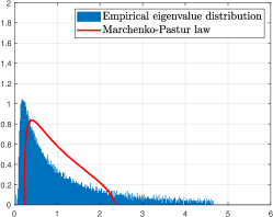
(d)

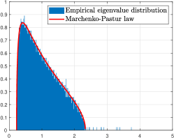
(e)

(f)

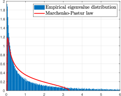
(g)

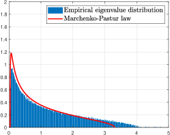
(h)

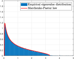
(i)

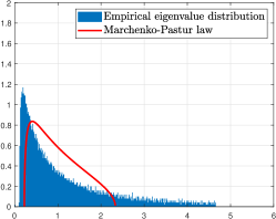
(j)

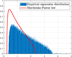
(k)

(l)

Figure 7: Empirical eigenvalue densities of scRNA-seq [64] and ST [44] data, before and after the normalization of the rows and columns. The scaling factors for the normalization were estimated using two approaches: 1) the QVF-based method of [39]; and 2) our proposed method (see Algorithm 1). The data was used either in its raw count form (panels (a) – (f)) or after a standard transformation (library normalization followed by mean subtraction; see the corresponding text).

5 Discussion

In this work, we developed an adaptive bi-diagonal scaling procedure for equalizing the average noise variance across the rows and columns of a given data matrix. We analyzed the accuracy of our proposed procedure in a wide range of settings and provided theoretical and empirical evidence of its advantages for signal detection and recovery under general heteroskedastic noise. Our approach is particularly appealing from a practical standpoint: it is fully automatic and data-driven, it supports general noise distributions and a broad range of signals and noise variance structures, and perhaps most importantly, it provides an empirical validation of our model assumptions via the accuracy of the spectrum’s fit to the MP law after normalization.

It is worthwhile to briefly discuss our delocalization assumption on the signal’s singular vectors (see Assumption 4 in Section 2.2 and the subsequent text). Currently, this assumption prohibits highly localized singular vectors, e.g., with a finite number of nonzeros or a logarithmically-growing number of them (with respect to the growing dimensions of the matrix). A natural question is whether this assumption is required in practice and whether it can be relaxed. We conjecture that some amount of delocalization of the signal singular vectors is always necessary to treat heteroskedastic noise with a general variance matrix $S$. Otherwise, a single row or column in the data with abnormally strong noise can always be considered as a rank-one component in the signal (see, e.g., Figure 1). In this case, there is no fundamental way of telling whether such a row or column belongs to the signal or the noise. Therefore, our approach implicitly assumes that highly localized singular vectors (i.e., whose energy is concentrated in a very small number of entries) belong to the noise and are thus suppressed by the normalization of the rows and columns. We believe that this is a desirable property for many applications.

Another question of interest is whether it is possible to accurately estimate the scaling factors $\mathbf{x}$ and $\mathbf{y}$ for general variance matrices $S$ without relying on their incoherence with respect to $\widetilde{S}$ (see Assumption 7 and Lemma 13 in Section 2.3). One potential direction is to consider an iterative application of our proposed normalization, i.e., to apply Algorithm 1 consecutively to its own output. Our results in Section 2.3 already show that the estimation error of the scaling factors improves if the scaling factors are close to vectors of all-ones. This fact implies that an iterative application of our normalization may improve the estimation accuracy if the previous round of normalization made the variance matrix closer to being doubly regular. We conducted preliminary numerical experiments of this idea, not reported in this work, which suggest that iterative application of Algorithm 1 can indeed improve the quality of normalization in challenging regimes where $S$ does not abide by our incoherence requirements. However, a comprehensive investigation of this idea, especially the numerical stability and convergence of the iterative procedure, is beyond the scope of this work.

Lastly, an important future research direction is to further establish the advantages of the normalization (2) for signal detection and recovery in general heteroskedastic settings. First, it is desirable to investigate the influence of this normalization on the spectral signal-to-noise ratio, beyond the case of Gaussian noise with $S=\mathbf{x}\mathbf{y}^{T}$ (which was considered in [41]). In particular, it is worthwhile to characterize the settings where the spectral signal-to-noise ratio improves, and by how much. Second, it is of interest to analyze the recovery accuracy of the signal $X$ by singular value thresholding or shrinkage after the normalization (2), identifying scenarios where the potential for improvement in recovery accuracy is substantial. We leave such extensions for future work.

6 Acknowledgements

The authors acknowledge funding support from NIH grants R01GM131642, UM1PA051410, R33DA047037, U54AG076043, U54AG079759, U01DA053628, P50CA121974, and R01GM135928.

Appendix A Experiment reproducibility details

A.1 Figure 1

In this figure, the signal $X$ is of rank $20$ with $10$ identical singular values given by $\sqrt{10^{3}n}$ and $10$ identical singular values given by $\sqrt{3n}$. The singular vectors were obtained by orthonormalizing independent random Gaussian vectors of suitable size. The noise matrix $E$ was generated as Gaussian homoskedastic with variance $1$, except that we amplified its last $5$ rows and $5$ columns by factors of $\sqrt{10}$ and $10$, respectively. Specifically, $E_{ij}\sim\mathcal{N}(0,S_{ij})$, $S=\mathbf{x}\mathbf{y}^{T}$, where $\mathbf{x}=[1,\ldots,1,10,10,10,10,10]^{T}$ and $\mathbf{y}=[1,\ldots,1,100,100,100,100,100]^{T}$.

A.2 Figure 2

In this figure, the signal $X$ was generated in the same way as described for Figure 1. The noise was generated according to $E_{ij}\sim\mathcal{N}(0,S_{ij})$, $S=AB$, where $A\in\mathbb{R}^{m\times 10}$, $B\in\mathbb{R}^{10\times n}$, and $A_{ij},B_{ij}\sim\operatorname{exp}\{\mathcal{N}(0,2)\}$. We then normalized $S$ by a scalar so that its average entry is $1$.

Appendix B Adapting to unknown global scaling of the noise

The analysis in Section 2 relies on Assumptions 2 and 5, which require a specific scaling of the moments of $E_{ij}$ with respect to the dimensions of the matrix. In particular, they require that the noise variances $S_{ij}$ scale like $n^{-1}$. These assumptions also imply, if we assume $0<d_{1}\leq m/n\leq d_{2}<1$ for some global constants $d_{1},d_{2}>0$, that with high probability, all singular values of $E$ are bounded from above and from below by positive global constants. Specifically,

$$c_{1}\leq\sigma_{i}\{E\}\leq c_{2},$$ (54)

for some constants $c_{1},c_{2}>0$, with probability approaching $1$ as $n\rightarrow\infty$. This fact is a consequence of Theorems 2.1, 2.4, and 2.9 from [2].

The scaling requirement on the noise variances $S_{ij}\propto n^{-1}$ and the boundedness of the noise singular values may not naturally hold in applications. To account for other scalings of the noise, suppose that instead of $Y$, we observe

$$Y^{{}^{\prime}}=\alpha(m,n)Y,$$ (55)

where $\alpha(m,n)$ is a scalar with an unknown dependence on the matrix dimensions $m$ and $n$.

Since $\alpha(m,n)$ is unknown, we propose to estimate it from the data. According to (54), the singular values of the scaled noise $\alpha(m,n)E$ are bounded with high probability from above and from below by constant multiples of $\alpha(m,n)$. Hence, we can correct for the unknown scaling $\alpha(m,n)$, up to a global constant, if we know the singular values of $\alpha(m,n)E$. Since we do not have access to these singular values, we estimate $\alpha(m,n)$ directly from the scaled data $Y^{{}^{\prime}}$. To this end, we propose to exploit the fact that the signal $X$ is low-rank by employing the median singular value of $Y^{{}^{\prime}}$, which is robust to low-rank perturbations of $Y^{{}^{\prime}}$ for sufficiently large $m$ and $n$. Specifically, since $Y^{{}^{\prime}}=\alpha(m,n)X+\alpha(m,n)E$, where the rank of $X$ is of fixed and independent of $m$ and $n$, Weyl’s inequality for singular values of sums of matrices (see Theorem 3.3.16 in [30]) together with (54) imply that

$$c_{1}\alpha(m,n)\leq\operatorname{Median}\{\sigma_{1}\{Y^{{}^{\prime}}\},\ldots,\sigma_{m}\{Y^{{}^{\prime}}\}\}\leq c_{2}\alpha(m,n),$$ (56)

with probability approaching $1$ as $n\rightarrow\infty$. Consequently, the median singular value of $Y^{{}^{\prime}}$ is proportional to $\alpha(m,n)$ with high probability for large $m$ and $n$. We can then divide $Y{{}^{\prime}}$ by its median singular value to attain the scaling of the noise required for the analysis in Section 2. Alternatively, we can simply take

$$\eta=\operatorname{Median}\left\{\sigma_{1}\{Y^{{}^{\prime}}\},\ldots,\sigma_{m}\{Y^{{}^{\prime}}\}\right\},$$ (57)

and proceed as usual – treating $Y^{{}^{\prime}}$ as $Y$. By doing so, $\hat{\mathbf{x}}$ and $\hat{\mathbf{y}}$ from (17) would automatically account for the factor $\alpha(m,n)$, and would concentrate around $\alpha(m,n)\mathbf{x}$ and $\alpha(m,n)\mathbf{y}$, respectively. This follows from the fact that according to (16), if we multiply $Y$ and $\eta$ each by $\alpha(m,n)$, then $\hat{\mathbf{g}}^{(1)}$ and $\hat{\mathbf{g}}^{(2)}$ would be divided by $\alpha(m,n)$, and consequently, $\hat{\mathbf{x}}$ and $\hat{\mathbf{y}}$ would each be multiplied by $\alpha(m,n)$. Overall, this discussion justifies Step 3 in Algorithm 1.

Appendix C Auxiliary results and definitions

C.1 Boundedness of $\mathbf{g}$

Lemma 17.

Let $m\leq n$ and suppose that there exists a global constant $C>0$ such that $S_{ij}\leq Cn^{-1}$ for all $i,j$. Then,

$$\left(\eta+\frac{C}{\eta}\right)^{-1}<\mathbf{g}_{i}<\frac{1}{\eta},$$ (58)

for all $i\in[m+n]$, where $\mathbf{g}$ is the solution to (9).

Proof.

According to (9) we have

$$\eta<\eta+(\mathcal{S}\mathbf{g})_{i}=\frac{1}{\mathbf{g}_{i}},$$ (59)

for all $i\in[m+n]$, where we used the fact that $\mathcal{S}\mathbf{g}$ is a positive vector. Therefore, we immediately obtain the upper bound in (58). Plugging this upper bound in (9) we obtain the lower bound

$$\mathbf{g}_{i}>\left({\eta+\frac{(\mathcal{S}\mathbf{1}_{m+n})_{i}}{\eta}}\right)^{-1},$$ (60)

for all $i=1,\ldots,m+n$, where $\mathbf{1}_{m+n}$ is a vector of $m+n$ ones. Lastly, the assumption $S_{ij}\leq Cn^{-1}$ implies that $(\mathcal{S}\mathbf{1}_{m+n})_{i}\leq C\max\{1,m/n\}\leq C$ for all $i=1,\ldots,m+n$ (since $m\leq n$), which completes the proof. ∎

C.2 Boundedness of $\mathbf{x}$ and $\mathbf{y}$ for $S=\mathbf{x}\mathbf{y}^{T}$

Lemma 18.

Let $m\leq n$ and $S=\mathbf{x}\mathbf{y}^{T}$. Suppose that there exists global constants $C,c>0$ such that $cn^{-1}\leq S_{ij}\leq Cn^{-1}$ for all $i\in[m]$ and $j\in[n]$. Then, under the normalization (12), we have

$$\frac{1}{\sqrt{m}}\left(\frac{c}{\sqrt{C}}\right)\left(1+\frac{C}{\eta^{2}}\right)^{-3/2} \leq\mathbf{x}_{i}\leq\frac{1}{\sqrt{m}}\left(\frac{C}{\sqrt{c}}\right)\left(1+\frac{C}{\eta^{2}}\right)^{3/2},$$ (61)

$$\frac{\sqrt{m}}{n}\left(\frac{c}{\sqrt{C}}\right)\left(1+\frac{C}{\eta^{2}}\right)^{-3/2} \leq\mathbf{y}_{j}\leq\frac{\sqrt{m}}{n}\left(\frac{C}{\sqrt{c}}\right)\left(1+\frac{C}{\eta^{2}}\right)^{3/2},$$ (62)

for all $i\in[m]$ and $j\in[n]$.

Proof.

According to (12) and Lemma 17, we have

$$c\left(\eta+\frac{C}{\eta}\right)^{-1}\leq\frac{c}{n}\sum_{j=1}^{n}\mathbf{g}_{j}^{(2)}\leq\left(S\mathbf{g}^{(2)}\right)_{i}=\mathbf{x}_{i}\left(\mathbf{y}^{T}\mathbf{g}^{(2)}\right)=\mathbf{x}_{i}\left(\mathbf{x}^{T}\mathbf{g}^{(1)}\right)\leq\frac{\mathbf{x}_{i}}{\eta}\sum_{k=1}^{m}\mathbf{x}_{k}.$$ (63)

Summing the above over $i=1,\ldots,m$ and taking the square root of both sides gives

$$\sum_{i=1}^{m}\mathbf{x}_{i}\geq m^{1/2}\sqrt{\frac{c\eta}{\eta+C\eta^{-1}}}.$$ (64)

Similarly, we have

$$\left(\eta+\frac{C}{\eta}\right)^{-1}\mathbf{x}_{i}\sum_{k=1}^{m}\mathbf{x}_{k}\leq\mathbf{x}_{i}\left(\mathbf{x}^{T}\mathbf{g}^{(1)}\right)=\mathbf{x}_{i}\left(\mathbf{y}^{T}\mathbf{g}^{(2)}\right)=\left(S\mathbf{g}^{(2)}\right)_{i}\leq\frac{C}{n}\sum_{j=1}^{n}\mathbf{g}_{j}^{(2)}\leq\frac{C}{\eta},$$ (65)

implying that

$$\sum_{i=1}^{m}\mathbf{x}_{i}\leq m^{1/2}\sqrt{\frac{C}{\eta}\left(\eta+\frac{C}{\eta}\right)}.$$ (66)

Combining all of the above and after some manipulation, we obtain that

$$\frac{1}{\sqrt{m}}\left(\frac{c}{\sqrt{C}}\right)\left(1+\frac{C}{\eta^{2}}\right)^{-3/2}\leq\mathbf{x}_{i}\leq\frac{1}{\sqrt{m}}\left(\frac{C}{\sqrt{c}}\right)\left(1+\frac{C}{\eta^{2}}\right)^{3/2},$$ (67)

for all $i\in[m]$. Next, we derive analogous bounds for $\mathbf{y}_{j}$. First, we have

$$c\left(\frac{m}{n}\right)\left(\eta+\frac{C}{\eta}\right)^{-1}\leq\frac{c}{n}\sum_{i=1}^{m}\mathbf{g}_{i}^{(1)}\leq\left([\mathbf{g}^{(1)}]^{T}S\right)_{j}=\left([\mathbf{g}^{(1)}]^{T}\mathbf{x}\right)\mathbf{y}_{j}=\left([\mathbf{g}^{(2)}]^{T}\mathbf{y}\right)\mathbf{y}_{j}\leq\frac{\mathbf{y}_{j}}{\eta}\sum_{k=1}^{n}\mathbf{y}_{k},$$ (68)

which asserts that

$$\sum_{j=1}^{n}\mathbf{y}_{j}\geq m^{1/2}\sqrt{\frac{c\eta}{\eta+C\eta^{-1}}}.$$ (69)

Second, we can write

$$\left(\eta+\frac{C}{\eta}\right)^{-1}\mathbf{y}_{j}\sum_{k=1}^{n}\mathbf{y}_{k}\leq\left([\mathbf{g}^{(2)}]^{T}\mathbf{y}\right)\mathbf{y}_{j}=\left([\mathbf{g}^{(1)}]^{T}\mathbf{x}\right)\mathbf{y}_{j}=\left([\mathbf{g}^{(1)}]^{T}S\right)_{j}\leq\left(\frac{C}{n}\right)\sum_{i=1}^{m}\mathbf{g}_{i}^{(1)}\leq\frac{C}{\eta}\left(\frac{m}{n}\right),$$ (70)

which leads to

$$\sum_{j=1}^{n}\mathbf{y}_{j}\leq m^{1/2}\sqrt{\frac{C}{\eta}\left(\eta+\frac{C}{\eta}\right)}.$$ (71)

Finally, combining the last four equations gives

$$\frac{\sqrt{m}}{n}\left(\frac{c}{\sqrt{C}}\right)\left(1+\frac{C}{\eta^{2}}\right)^{-3/2}\leq\mathbf{y}_{j}\leq\frac{\sqrt{m}}{n}\left(\frac{C}{\sqrt{c}}\right)\left(1+\frac{C}{\eta^{2}}\right)^{3/2},$$ (72)

for all $j\in[n]$. ∎

C.3 Boundedness of $\mathbf{x}$ and $\mathbf{y}$ for general $S$

Lemma 19.

Let $m\leq n$ and suppose there exists global constants $C,c>0$ such that $cn^{-1}\leq S_{ij}\leq Cn^{-1}$ for all $i\in[m]$ and $j\in[n]$. Then, under the normalization (30), we have

$$\frac{1}{\sqrt{m}}\left(\frac{c^{5/2}}{{C^{2}}}\right)\left(1+\frac{C^{2}}{c\eta^{2}}\right)^{-3/2} \leq\mathbf{x}_{i}\leq\frac{1}{\sqrt{m}}\left(\frac{C^{5/2}}{{c^{2}}}\right)\left(1+\frac{C^{2}}{c\eta^{2}}\right)^{3/2},$$ (73)

$$\frac{\sqrt{m}}{n}\left(\frac{c^{5/2}}{{C^{2}}}\right)\left(1+\frac{C^{2}}{c\eta^{2}}\right)^{-3/2} \leq\mathbf{y}_{j}\leq\frac{\sqrt{m}}{n}\left(\frac{C^{5/2}}{{c^{2}}}\right)\left(1+\frac{C^{2}}{c\eta^{2}}\right)^{3/2},$$ (74)

for all $i\in[m]$ and $j\in[n]$.

Proof.

According to (28) we can write

$$\widetilde{S}_{ij}=\frac{S_{ij}}{\mathbf{x}_{i}\mathbf{y}_{j}},$$ (75)

where the sum of each row of $\widetilde{S}$ is $n$ and the sum of each column of $\widetilde{S}$ is $m$. Therefore, applying Lemma 4.1 in [38] together with the assumptions in Lemma 19, we obtain

$$\frac{c}{C^{2}}n\leq\frac{1}{\mathbf{x}_{i}\mathbf{y}_{j}}\leq\frac{C}{c^{2}}n,$$ (76)

implying that

$$\frac{c^{2}}{C}n^{-1}\leq{\mathbf{x}_{i}\mathbf{y}_{j}}\leq\frac{C^{2}}{c}n^{-1}.$$ (77)

Note that the normalization (30) is equivalent to (12) under Assumption 1 ($S=\mathbf{x}\mathbf{y}^{T}$). Since the proof of Lemma 18 relies on the assumption $cn^{-1}\leq\mathbf{x}_{i}\mathbf{y}_{j}\leq Cn^{-1}$, it also holds in the setting of this lemma if we replace $c$ and $C$ in the statement of Lemma 18 with $c^{2}/C$ and $C^{2}/c$, respectively, which provides the required result. ∎

C.4 Stability of the Dyson equation on the imaginary axis

Lemma 20.

Let $\widetilde{\mathbf{g}}\in\mathbb{R}^{m+n}$ be a positive vector satisfying

$$\frac{1}{\widetilde{\mathbf{g}}}=\eta+\mathcal{S}\widetilde{\mathbf{g}}+\mathbf{e},$$ (78)

for some $\mathbf{e}\in\mathbb{R}^{m+n}$. Then,

$$\left\|\frac{\widetilde{\mathbf{g}}-\mathbf{g}}{\mathbf{g}}\right\|_{\infty}\leq\|\mathbf{e}\|_{\infty}\max_{i}\{\widetilde{\mathbf{g}}_{i}\}\max\left\{1,\frac{2}{\eta\min_{i}\{\widetilde{\mathbf{g}}_{i}\}}\right\},$$ (79)

where $\mathbf{g}$ is the solution to (9).

Proof.

According to (78) we can write

$$1-D\{\widetilde{\mathbf{g}}\}\mathbf{e} =\eta\widetilde{\mathbf{g}}+D\{\widetilde{\mathbf{g}}\}\mathcal{S}\widetilde{\mathbf{g}}=\eta\widetilde{\mathbf{g}}+D\left\{\frac{\widetilde{\mathbf{g}}}{\mathbf{g}}\right\}D\{{\mathbf{g}}\}\mathcal{S}D\{{\mathbf{g}}\}\left[\frac{\widetilde{\mathbf{g}}}{\mathbf{g}}\right]$$

$$\geq\eta\widetilde{\mathbf{g}}+\min_{i}\left\{\frac{\widetilde{\mathbf{g}}_{i}}{\mathbf{g}_{i}}\right\}D\left\{\frac{\widetilde{\mathbf{g}}}{\mathbf{g}}\right\}D\{{\mathbf{g}}\}\mathcal{S}\mathbf{g}$$

$$=\eta\widetilde{\mathbf{g}}\left(1-\min_{i}\left\{\frac{\widetilde{\mathbf{g}}_{i}}{\mathbf{g}_{i}}\right\}\right)+\left[\frac{\widetilde{\mathbf{g}}}{\mathbf{g}}\right]\min_{i}\left\{\frac{\widetilde{\mathbf{g}}_{i}}{\mathbf{g}_{i}}\right\},$$ (80)

where we used $\mathcal{S}\mathbf{g}=1/\mathbf{g}-\eta$ (see (9)) in the last transition. Similarly, we have

$$1-D\{\widetilde{\mathbf{g}}\}\mathbf{e}\leq\eta\widetilde{\mathbf{g}}\left(1-\max_{i}\left\{\frac{\widetilde{\mathbf{g}}_{i}}{\mathbf{g}_{i}}\right\}\right)+\left[\frac{\widetilde{\mathbf{g}}}{\mathbf{g}}\right]\max_{i}\left\{\frac{\widetilde{\mathbf{g}}_{i}}{\mathbf{g}_{i}}\right\}.$$ (81)

Let us denote

$$k=\operatorname{argmax}_{i\in[m+n]}\left\{\frac{\widetilde{\mathbf{g}}_{i}}{\mathbf{g}_{i}}\right\},\qquad\ell=\operatorname{argmin}_{i\in[m+n]}\left\{\frac{\widetilde{\mathbf{g}}_{i}}{\mathbf{g}_{i}}\right\}.$$ (82)

Using (80) we obtain

$$1+\widetilde{\mathbf{g}}_{k}|\mathbf{e}_{k}|\geq 1-\widetilde{\mathbf{g}}_{k}\mathbf{e}_{k}\geq\eta\widetilde{\mathbf{g}}_{k}\left(1-\min_{i}\left\{\frac{\widetilde{\mathbf{g}}_{i}}{\mathbf{g}_{i}}\right\}\right)+\max_{i}\left\{\frac{\widetilde{\mathbf{g}}_{i}}{\mathbf{g}_{i}}\right\}\min_{i}\left\{\frac{\widetilde{\mathbf{g}}_{i}}{\mathbf{g}_{i}}\right\},$$ (83)

and analogously, using (81) we have

$$1-\widetilde{\mathbf{g}}_{\ell}|\mathbf{e}_{\ell}|\leq 1-\widetilde{\mathbf{g}}_{\ell}\mathbf{e}_{\ell}\leq\eta\widetilde{\mathbf{g}}_{\ell}\left(1-\max_{i}\left\{\frac{\widetilde{\mathbf{g}}_{i}}{\mathbf{g}_{i}}\right\}\right)+\max_{i}\left\{\frac{\widetilde{\mathbf{g}}_{i}}{\mathbf{g}_{i}}\right\}\min_{i}\left\{\frac{\widetilde{\mathbf{g}}_{i}}{\mathbf{g}_{i}}\right\}.$$ (84)

Subtracting one of the two equations above from the other implies that

$$\widetilde{\mathbf{g}}_{k}\left(1-\min_{i}\left\{\frac{\widetilde{\mathbf{g}}_{i}}{\mathbf{g}_{i}}\right\}\right)+\widetilde{\mathbf{g}}_{\ell}\left(\max_{i}\left\{\frac{\widetilde{\mathbf{g}}_{i}}{\mathbf{g}_{i}}\right\}-1\right)\leq\frac{\widetilde{\mathbf{g}}_{k}|\mathbf{e}_{k}|+\widetilde{\mathbf{g}}_{\ell}|\mathbf{e}_{\ell}|}{\eta},$$ (85)

and consequently,

$$\left(1-\min_{i}\left\{\frac{\widetilde{\mathbf{g}}_{i}}{\mathbf{g}_{i}}\right\}\right)+\left(\max_{i}\left\{\frac{\widetilde{\mathbf{g}}_{i}}{\mathbf{g}_{i}}\right\}-1\right)\leq\frac{2\|\mathbf{e}\|_{\infty}}{\eta}\left(\frac{\max_{i}\{\widetilde{\mathbf{g}}_{i}\}}{\min_{i}\{\widetilde{\mathbf{g}}_{i}\}}\right).$$ (86)

Next, we consider four different cases that correspond to the possible signs of the two summands in the left-hand side of (86):

1. $\min_{i}\left\{{\widetilde{\mathbf{g}}_{i}}/{\mathbf{g}_{i}}\right\}\leq 1$ and $\max_{i}\left\{{\widetilde{\mathbf{g}}_{i}}/{\mathbf{g}_{i}}\right\}\geq 1$: In this case, both summands in the left-hand side of (86) are nonnegative, thus

   $$-\frac{2\|\mathbf{e}\|_{\infty}}{\eta}\left(\frac{\max_{i}\{\widetilde{\mathbf{g}}_{i}\}}{\min_{i}\{\widetilde{\mathbf{g}}_{i}\}}\right)\leq\min_{i}\left\{\frac{\widetilde{\mathbf{g}}_{i}}{\mathbf{g}_{i}}\right\}-1\leq\frac{\widetilde{\mathbf{g}}_{i}}{\mathbf{g}_{i}}-1\leq\max_{i}\left\{\frac{\widetilde{\mathbf{g}}_{i}}{\mathbf{g}_{i}}\right\}-1\leq\frac{2\|\mathbf{e}\|_{\infty}}{\eta}\left(\frac{\max_{i}\{\widetilde{\mathbf{g}}_{i}\}}{\min_{i}\{\widetilde{\mathbf{g}}_{i}\}}\right),$$ (87)

   for all $i\in[m+n]$.

2. $\min_{i}\left\{{\widetilde{\mathbf{g}}_{i}}/{\mathbf{g}_{i}}\right\}\leq 1$ and $\max_{i}\left\{{\widetilde{\mathbf{g}}_{i}}/{\mathbf{g}_{i}}\right\}<1$: In this case we have $\widetilde{\mathbf{g}}_{i}<\mathbf{g}_{i}$ for all $i\in[m+n]$, and therefore we can use (9) to write

   $$\frac{1}{\mathbf{g}}=\eta+\mathcal{S}\mathbf{g}>\eta+\mathcal{S}\widetilde{\mathbf{g}}=\frac{1}{\widetilde{\mathbf{g}}}-\mathbf{e},$$ (88)

   where we used (78) in the last transition. Consequently, we obtain

   $$1>\frac{\widetilde{\mathbf{g}}_{i}}{\mathbf{g}_{i}}>1-\widetilde{\mathbf{g}}_{i}\mathbf{e}_{i}\geq 1-\|\mathbf{e}\|_{\infty}\max_{i}\{\widetilde{\mathbf{g}}_{i}\},$$ (89)

   for all $i\in[m+n]$.

3. $\min_{i}\left\{{\widetilde{\mathbf{g}}_{i}}/{\mathbf{g}_{i}}\right\}>1$ and $\max_{i}\left\{{\widetilde{\mathbf{g}}_{i}}/{\mathbf{g}_{i}}\right\}\geq 1$: In this case we have $\widetilde{\mathbf{g}}_{i}>\mathbf{g}_{i}$ for all $i\in[m+n]$, and therefore we can use (9) to write

   $$\frac{1}{\mathbf{g}}=\eta+\mathcal{S}\mathbf{g}<\eta+\mathcal{S}\widetilde{\mathbf{g}}=\frac{1}{\widetilde{\mathbf{g}}}-\mathbf{e},$$ (90)

   where we used (78) in the last transition. Consequently, we obtain

   $$1<\frac{\widetilde{\mathbf{g}}_{i}}{\mathbf{g}_{i}}<1-\widetilde{\mathbf{g}}_{i}\mathbf{e}_{i}\leq 1+\|\mathbf{e}\|_{\infty}\max_{i}\{\widetilde{\mathbf{g}}_{i}\},$$ (91)

   for all $i\in[m+n]$.

4. $\min_{i}\left\{{\widetilde{\mathbf{g}}_{i}}/{\mathbf{g}_{i}}\right\}>1$ and $\max_{i}\left\{{\widetilde{\mathbf{g}}_{i}}/{\mathbf{g}_{i}}\right\}<1$: This case is clearly infeasible.

Overall, considering all possible cases mentioned above, we conclude that

$$\left|\frac{\widetilde{\mathbf{g}}_{i}}{\mathbf{g}_{i}}-1\right|\leq\|\mathbf{e}\|_{\infty}\max_{i}\{\widetilde{\mathbf{g}}_{i}\}\max\left\{1,\frac{2}{\eta\min_{i}\{\widetilde{\mathbf{g}}_{i}\}}\right\},$$ (92)

for all $i\in[m+n]$.

∎

C.5 Order with high probability

For simplicity of presentation and brevity of our proofs, we will make use of the following definition.

Definition 21.

Let $X$ be a complex-valued random variable. We say that $X=\mathcal{O}_{n}\left(f(m,n)\right)$ if there exist $C^{{}^{\prime}},c^{{}^{\prime}}(t)>0$, such that with probability at least $1-c^{{}^{\prime}}(t)n^{-t}$, for all $t>0$,

$$|X|\leq C^{{}^{\prime}}f(m,n).$$ (93)

The following two facts make it easy to analyze expressions involving multiple variables satisfying Definition 21 and functions thereof.

1. Let $X_{1},X_{2},\ldots,X_{P(n)}$ be random variables satisfying $X_{i}=\mathcal{O}_{n}(f(m,n))$, where $P(n)$ is a polynomial in $n$. Then, by Definition 21, applying the union bound $P(n)$ times yields

   $$\max_{i=1,\ldots,P(n)}|X_{i}|=\mathcal{O}_{n}(f(m,n)).$$ (94)

2. Let $X$ be a real-valued random variable satisfying $X=\mathcal{O}_{n}(f(m,n))$ and define $Y=g(X)$, where $g:\mathbb{R}\rightarrow\mathbb{R}$ is a differentiable function in a neighborhood of zero. Suppose that $\lim_{n\rightarrow\infty}f(m,n)=0$ and that the first derivative of $g(\cdot)$ is uniformly bounded by a global constant in a neighborhood of zero. Then, by Definition 21 and the Taylor expansion of $g(\cdot)$ around zero, it follows that

   $$Y=g(0)+\mathcal{O}_{n}(f(m,n)).$$ (95)

We will use the above two properties of Definition 21 seamlessly throughout our proofs below.

Appendix D Proof of Lemma 5

Under Assumption 2, we can apply Theorem 2.1 in [14], noting that Assumptions $A$ and $CD$ in [14] are satisfied in our setting since the noise entries $E_{ij}$ are independent and have zero means. Theorem 2.1 in [14] states that for any $\epsilon>0$ there exists $\delta,C_{0},C_{1}(\epsilon,t)>0$ such that for all $t>0$, $i\in[m+n]$, and $z\in\{z:\operatorname{Im}(z)\geq(m+n)^{-\delta},\;|z|\leq(m+n)^{C_{0}}\}$, with probability at least $1-C_{1}(\epsilon,D)n^{-t}$,

$$|\mathbf{a}^{T}R(z)\mathbf{b}-\mathbf{a}^{T}M\mathbf{b}|\leq\frac{(m+n)^{\epsilon-1/2}}{(1+|z|)^{2}}.$$ (96)

Here, $M\in\mathbb{C}^{(m+n)\times(m+n)}$ is the solution to a certain matrix-valued Dyson equation appearing in [14], $C_{0}\geq 100$ is universal constant, and $C_{1}(\epsilon,t)$ is a constant depending on $\epsilon$, $t$, and on the universal constants in Assumption 2. It is easy to verify from [14] that since $E_{ij}$ are independent with zero means, the matrix $M$ (solving the matrix Dyson equation appearing in [14]) is a diagonal matrix whose main diagonal is precisely $\mathbf{f}$ from (7), i.e., $M=D\{\mathbf{f}(z)\}$; see also [2]. If we take $z=\imath\eta$, then $\mathbf{f}(z)=\imath\mathbf{g}(\eta)$. Note that the aforementioned condition $z\in\{z:\operatorname{Im}(z)\geq(m+n)^{-\delta},\;|z|\leq(m+n)^{C_{0}}\}$ is satisfied for any fixed $\eta>0$ if $n$ is sufficiently large, namely if $n\geq n_{0}$ for some constant $n_{0}$ that may depend on $\eta$ and $\epsilon$ (since $\delta$ is determined by $\epsilon$). We can always represent the requirement $n\geq n_{0}$ in our Definition 21 by taking $c{{}^{\prime}}(t)$ to be large enough so that $1-c^{{}^{\prime}}(t)n^{-t}\leq 0$ for all $n<n_{0}$, e.g., $c^{{}^{\prime}}(t)=\max\{n_{0}^{t},C_{1}(\epsilon,t)\}$. Finally, the required result follows from the fact that $n\leq m+n\leq 2n$ (since $0\leq m\leq n$ in our setup).

Appendix E Proof of Proposition 2

Plugging $S=\mathbf{x}\mathbf{y}^{T}$ into the system of coupled equations (10), we can write

$$\mathbf{x}=\frac{1}{\mathbf{y}^{T}\mathbf{g}^{(2)}}\left(\frac{1}{\mathbf{g}^{(1)}}-\eta\right),\qquad\qquad\mathbf{y}=\frac{1}{\mathbf{x}^{T}\mathbf{g}^{(1)}}\left(\frac{1}{\mathbf{g}^{(2)}}-\eta\right).$$ (97)

Therefore, by transposing the two equations above and multiplying them by $\mathbf{g}^{(1)}$ and $\mathbf{g}^{(2)}$, respectively, we obtain

$$\mathbf{x}^{T}\mathbf{g}^{(1)}=\frac{n-\eta\|\mathbf{g}^{(1)}\|_{1}}{\mathbf{y}^{T}\mathbf{g}^{(2)}},\qquad\qquad\mathbf{y}^{T}\mathbf{g}^{(2)}=\frac{m-\eta\|\mathbf{g}^{(2)}\|_{1}}{\mathbf{x}^{T}\mathbf{g}^{(1)}},$$ (98)

implying that

$$(\mathbf{x}^{T}\mathbf{g}^{(1)})(\mathbf{y}^{T}\mathbf{g}^{(2)})=n-\eta\|\mathbf{g}^{(1)}\|_{1}=m-\eta\|\mathbf{g}^{(2)}\|_{1}.$$ (99)

Consequently, using the definition of $\alpha$ from (11), we can rewrite $\mathbf{x}$ and $\mathbf{y}$ as

$$\mathbf{x}=\frac{\alpha}{\sqrt{\left(\mathbf{y}^{T}\mathbf{g}^{(2)}\right)\left(\mathbf{x}^{T}\mathbf{g}^{(1)}\right)}}\left(\frac{1}{\mathbf{g}^{(1)}}-\eta\right),\qquad\qquad\mathbf{y}=\frac{\alpha^{-1}}{\sqrt{\left(\mathbf{y}^{T}\mathbf{g}^{(2)}\right)\left(\mathbf{x}^{T}\mathbf{g}^{(1)}\right)}}\left(\frac{1}{\mathbf{g}^{(2)}}-\eta\right),$$ (100)

which together with (99) completes the proof.

Appendix F Proof of Proposition 3

Let $V=[V^{(1)},V^{(2)}]$, where $V^{(1)}\in\mathbb{R}^{n\times m}$ and $V^{(2)}\in\mathbb{R}^{n\times(n-m)}$, and denote $\Sigma=D\{\sigma_{1},\ldots,\sigma_{m}\}\in\mathbb{R}^{m\times m}$. We can write the eigen-decomposition of $\mathcal{Y}$ as

$$\mathcal{Y}=\begin{bmatrix}\frac{1}{\sqrt{2}}U&\frac{1}{\sqrt{2}}U&\mathbf{0}\\ \frac{1}{\sqrt{2}}V^{(1)}&-\frac{1}{\sqrt{2}}V^{(1)}&{V}^{(2)}\end{bmatrix}\begin{bmatrix}\Sigma&\mathbf{0}&\mathbf{0}\\ \mathbf{0}&-\Sigma&\mathbf{0}\\ \mathbf{0}&\mathbf{0}&\mathbf{0}\end{bmatrix}\begin{bmatrix}\frac{1}{\sqrt{2}}U&\frac{1}{\sqrt{2}}U&\mathbf{0}\\ \frac{1}{\sqrt{2}}V^{(1)}&-\frac{1}{\sqrt{2}}V^{(1)}&{V}^{(2)}\end{bmatrix}^{T},$$ (101)

where $\mathbf{0}$ is a block of zeros of suitable size. Consequently, the resolvent of $\mathcal{Y}$ from (14) is given by

$$\mathcal{R}(z)=\begin{bmatrix}\frac{1}{\sqrt{2}}U&\frac{1}{\sqrt{2}}U&\mathbf{0}\\ \frac{1}{\sqrt{2}}V^{(1)}&-\frac{1}{\sqrt{2}}V^{(1)}&{V}^{(2)}\end{bmatrix}\begin{bmatrix}(\Sigma-zI)^{-1}&\mathbf{0}&\mathbf{0}\\ \mathbf{0}&(-\Sigma-zI)^{-1}&\mathbf{0}\\ \mathbf{0}&\mathbf{0}&-z^{-1}I\end{bmatrix}\begin{bmatrix}\frac{1}{\sqrt{2}}U&\frac{1}{\sqrt{2}}U&\mathbf{0}\\ \frac{1}{\sqrt{2}}V^{(1)}&-\frac{1}{\sqrt{2}}V^{(1)}&{V}^{(2)}\end{bmatrix}^{T}.$$ (102)

If we denote the top left $m\times m$ block of $\mathcal{R}$ by $\mathcal{R}^{(11)}$, then a direct calculation shows that

$$\hat{\mathbf{g}}^{(1)}_{i}=\operatorname{Im}\{\mathcal{R}^{(11)}_{ii}(\imath\eta)\}=\frac{1}{2}\sum_{k=1}^{m}U_{ik}^{2}\operatorname{Im}\left\{\frac{1}{\sigma_{k}-\imath\eta}+\frac{1}{-\sigma_{k}-\imath\eta}\right\}=\sum_{k=1}^{m}U_{ik}^{2}\frac{\eta}{\sigma_{k}^{2}+\eta^{2}},$$ (103)

for all $i\in[m]$. Similarly, denoting the bottom right $n\times n$ block $\mathcal{R}$ by $\mathcal{R}^{(22)}$, we have

$$\hat{\mathbf{g}}^{(2)}_{j} =\operatorname{Im}\{\mathcal{R}^{(22)}_{jj}(\imath\eta)\}=\frac{1}{2}\sum_{k=1}^{m}(V_{jk}^{(1)})^{2}\operatorname{Im}\left\{\frac{1}{\sigma_{k}-\imath\eta}+\frac{1}{-\sigma_{k}-\imath\eta}\right\}+\frac{1}{\eta}\sum_{k=1}^{n-m}(V_{jk}^{(2)})^{2}$$ (104)

$$=\frac{1}{\eta}+\sum_{k=1}^{m}V_{jk}^{2}\left(\frac{\eta}{\sigma_{k}^{2}+\eta^{2}}-\frac{1}{\eta}\right),$$ (105)

for all $j\in[n]$, where we used the fact that $\sum_{k=1}^{n-m}(V_{jk}^{(2)})^{2}=1-\sum_{k=1}^{m}(V_{jk}^{(1)})^{2}$.

Appendix G Proof of Proposition 4

Since $0\leq\sigma_{k}<\infty$ and $U$ and $V$ are orthogonal matrices, it follows from (17) that $0<\hat{\mathbf{g}}_{i}^{(1)}\leq 1/\eta$ and $0<\hat{\mathbf{g}}_{j}^{(2)}\leq 1/\eta$ for all $i\in[m]$ and $j\in[n]$. Therefore, according to (17), the only situation where the vectors $\hat{\mathbf{x}}$ and $\hat{\mathbf{y}}$ are ill-posed is if $\hat{\mathbf{g}}^{(1)}=\mathbf{1}_{m}/\eta$ or $\hat{\mathbf{g}}^{(2)}=\mathbf{1}_{n}/\eta$, respectively. According to (16), this can only happen if $\sigma_{1}=\ldots=\sigma_{m}=0$, i.e., if $Y$ is the zero matrix $\mathbf{0}_{m\times n}$. Otherwise, we must have $\hat{\mathbf{x}}_{i}\geq 0$ and $\hat{\mathbf{y}}_{j}\geq 0$ for all $i\in[m]$ and $j\in[n]$. We now consider the positivity of $\hat{\mathbf{x}}$ and $\hat{\mathbf{y}}$. Let us fix $i\in[m]$. If there exists $k\in[m]$ such that $\sigma_{k}>0$ and $U_{ik}^{2}>0$, then we obtain the strict inequality $\hat{\mathbf{g}}_{i}^{(1)}<1/\eta$, which implies that $\hat{\mathbf{x}}_{i}>0$. Otherwise, we must have that $U_{ik}=0$ for all $k\in[m]$ for which $\sigma_{k}>0$, asserting, by the SVD of $Y$, that $Y_{ij}=0$ for all $j\in[n]$, i.e., the $i$’th row of $Y$ is entirely zero. Conversely, if the $i$’th row of $Y$ is entirely zero, then $U_{ik}=0$ for all $k\in[m]$ with $\sigma_{k}>0$, implying that $\hat{\mathbf{g}}^{(1)}_{i}=1/\eta$ and hence $\hat{\mathbf{x}}_{i}=0$. An analogous argument establishes that $\hat{\mathbf{y}}_{j}=0$ if and only if the $j$’th column of $Y$ is zero.

Appendix H Proof of Theorem 6

Let us define the matrices $\mathcal{X}\in\mathbb{R}^{(m+n)\times(m+n)}$, $\mathcal{U}\in\mathbb{R}^{(m+n)\times 2r}$, and $\mathcal{V}\in\mathbb{R}^{(m+n)\times 2r}$, as

$$\mathcal{X}=\begin{bmatrix}\mathbf{0}&X\\ X^{T}&\mathbf{0}\end{bmatrix},\quad\mathcal{U}=\begin{bmatrix}\widetilde{U}&\mathbf{0}\\ \mathbf{0}&\widetilde{V}\end{bmatrix},\quad\mathcal{V}=\begin{bmatrix}\mathbf{0}&\widetilde{U}\\ \widetilde{V}&\mathbf{0}\end{bmatrix},\quad\Sigma=\begin{bmatrix}D\{s_{1},\ldots,s_{r}\}&\mathbf{0}\\ \mathbf{0}&D\{s_{1},\ldots,s_{r}\}\end{bmatrix}.$$ (106)

We can therefore write $\mathcal{X}=\mathcal{U}\Sigma\mathcal{V}^{T}$, and we have

$$\mathcal{R}(z)=\left(\mathcal{X}+\mathcal{E}-zI\right)^{-1}=\left(\mathcal{E}-zI+\mathcal{U}\Sigma\mathcal{V}^{T}\right)^{-1}=\left(R^{-1}(z)+\mathcal{U}\Sigma\mathcal{V}^{T}\right)^{-1}.$$ (107)

Using the Woodbury matrix identity, we obtain

$$\mathcal{R}(z)=R(z)+R(z)\mathcal{U}\left(\Sigma^{-1}+\mathcal{V}^{T}R(z)\mathcal{U}\right)^{-1}\mathcal{V}^{T}R(z).$$ (108)

Taking $z=\imath\eta$ and applying Lemma 5, we have

$$[R(\imath\eta)\mathcal{U}]_{ij} =\imath[D\{\mathbf{g}\}\mathcal{U}]_{ij}+\mathcal{O}_{n}(n^{\epsilon-1/2})$$

$$=\imath\begin{bmatrix}D\{\mathbf{g}^{(1)}\}\widetilde{U}&\mathbf{0}\\ \mathbf{0}&D\{\mathbf{g}^{(2)}\}\widetilde{V}\end{bmatrix}_{ij}+\mathcal{O}_{n}(n^{\epsilon-1/2}),$$ (109)

$$[\mathcal{V}^{T}R(\imath\eta)]_{ji} =\imath[\mathcal{V}^{T}D\{\mathbf{g}\}]_{ji}+\mathcal{O}_{n}(n^{\epsilon-1/2})$$

$$=\imath\begin{bmatrix}\mathbf{0}&\widetilde{V}^{T}D\{\mathbf{g}^{(2)}\}\\ \widetilde{U}^{T}D\{\mathbf{g}^{(1)}\}&\mathbf{0}\end{bmatrix}_{ji}+\mathcal{O}_{n}(n^{\epsilon-1/2}),$$ (110)

for all $i\in[m+n]$ and $j\in[2r]$. Let us define

$$A=\begin{bmatrix}A_{11}&A_{12}\\ A_{21}&A_{22}\end{bmatrix}=\left(\Sigma^{-1}+\mathcal{V}^{T}R(z)\mathcal{U}\right)^{-1},$$ (111)

where $A_{11},A_{12},A_{21},A_{22}\in\mathbb{C}^{r\times r}$. By plugging (111), (109), and (110) into (108) to evaluate $\mathcal{R}_{ii}(z)$ at $z=\imath\eta$, we get

$$\mathcal{R}_{ii}(\imath\eta) =R_{ii}(\imath\eta)+[R(\imath\eta)\mathcal{U}A\mathcal{V}^{T}R(\imath\eta)]_{ii}$$

$$=R_{ii}(\imath\eta)-\left(\begin{bmatrix}D\{\mathbf{g}^{(1)}\}\widetilde{U}&\mathbf{0}\\ \mathbf{0}&D\{\mathbf{g}^{(2)}\}\widetilde{V}\end{bmatrix}\begin{bmatrix}A_{11}&A_{12}\\ A_{21}&A_{22}\end{bmatrix}\begin{bmatrix}\mathbf{0}&\widetilde{V}^{T}D\{\mathbf{g}^{(2)}\}\\ \widetilde{U}^{T}D\{\mathbf{g}^{(1)}\}&\mathbf{0}\end{bmatrix}\right)_{ii}$$

$$+\eta^{(1)}_{i}+\eta^{(2)}_{i}+\eta^{(3)}_{i},$$ (112)

where

$$|\eta^{(1)}_{i}| \leq\mathcal{O}_{n}(n^{\epsilon-1/2})\|A\|_{2}\left\|\begin{bmatrix}\mathbf{0}&\widetilde{V}^{T}D\{\mathbf{g}^{(2)}\}\\ \widetilde{U}^{T}D\{\mathbf{g}^{(1)}\}&\mathbf{0}\end{bmatrix}\right\|_{2},$$ (113)

$$|\eta^{(2)}_{i}| \leq\mathcal{O}_{n}(n^{\epsilon-1/2})\|A\|_{2}\left\|\begin{bmatrix}D\{\mathbf{g}^{(1)}\}\widetilde{U}&\mathbf{0}\\ \mathbf{0}&D\{\mathbf{g}^{(2)}\}\widetilde{V}\end{bmatrix}\right\|_{2},$$ (114)

$$|\eta^{(3)}_{i}| \leq\mathcal{O}_{n}(n^{2\epsilon-1})\|A\|_{2}.$$ (115)

Since the columns of $\widetilde{U}$ and $\widetilde{V}$ are orthonormal, it follows that

$$\left\|\begin{bmatrix}\mathbf{0}&\widetilde{V}^{T}D\{\mathbf{g}^{(2)}\}\\ \widetilde{U}^{T}D\{\mathbf{g}^{(1)}\}&\mathbf{0}\end{bmatrix}\right\|_{2}\leq\left\|\begin{bmatrix}\mathbf{0}&\widetilde{V}^{T}\\ \widetilde{U}^{T}&\mathbf{0}\end{bmatrix}\right\|_{2}\|D\{\mathbf{g}\}\|_{2}\leq\|\mathbf{g}\|_{\infty}\leq\frac{1}{\eta},$$ (116)

$$\left\|\begin{bmatrix}D\{\mathbf{g}^{(1)}\}\widetilde{U}&\mathbf{0}\\ \mathbf{0}&D\{\mathbf{g}^{(2)}\}\widetilde{V}\end{bmatrix}\right\|_{2}\leq\left\|\begin{bmatrix}\widetilde{U}&\mathbf{0}\\ \mathbf{0}&\widetilde{V}\end{bmatrix}\right\|_{2}\|D\{\mathbf{g}\}\|_{2}\leq\|\mathbf{g}\|_{\infty}\leq\frac{1}{\eta},$$ (117)

where we used Lemma 17 in the last transition. Let us define $\eta^{(4)}=\eta^{(1)}+\eta^{(2)}+\eta^{(3)}$, which satisfies

$$\|\eta^{(4)}\|_{\infty}\leq\mathcal{O}_{n}(n^{\epsilon-1/2})\|A\|_{2}.$$ (118)

We can now write

$$\hat{\mathbf{g}}_{i} =\operatorname{Im}\{\mathcal{R}_{ii}(\imath\eta)\}=\operatorname{Im}\{{R}_{ii}(\imath\eta)\}+\eta_{i}^{(4)}$$

$$-\operatorname{Im}\left\{\begin{bmatrix}D\{\mathbf{g}^{(1)}\}\widetilde{U}A_{12}\widetilde{U}^{T}D\{\mathbf{g}^{(1)}\}&D\{\mathbf{g}^{(1)}\}\widetilde{U}A_{11}\widetilde{V}^{T}D\{\mathbf{g}^{(2)}\}\\ D\{\mathbf{g}^{(2)}\}\widetilde{V}A_{22}\widetilde{U}^{T}D\{\mathbf{g}^{(1)}\}&D\{\mathbf{g}^{(2)}\}\widetilde{V}A_{21}\widetilde{V}^{T}D\{\mathbf{g}^{(2)}\}\end{bmatrix}\right\}_{ii}$$

$$={\mathbf{g}}_{i}+\mathcal{O}_{n}(n^{\epsilon-1/2})+\operatorname{Im}\{\eta_{i}^{(4)}\}-\begin{dcases}\operatorname{Im}\left\{\left[D\{\mathbf{g}^{(1)}\}\widetilde{U}A_{12}\widetilde{U}^{T}D\{\mathbf{g}^{(1)}\}\right]_{ii}\right\},&1\leq i\leq m,\\ \operatorname{Im}\left\{\left[D\{\mathbf{g}^{(2)}\}\widetilde{V}A_{21}\widetilde{V}^{T}D\{\mathbf{g}^{(2)}\}\right]_{ii}\right\},&m+1\leq i\leq m+n,\end{dcases}$$ (119)

for all $i\in[m+n]$, where we also used Lemma 5 in the last transition. Utilizing Lemma 17, we have

$$\left|\operatorname{Im}\left\{\left[D\{\mathbf{g}^{(1)}\}\widetilde{U}A_{12}\widetilde{U}^{T}D\{\mathbf{g}^{(1)}\}\right]_{ii}\right\}\right| \leq|\mathbf{g}_{i}^{(1)}|^{2}\|A_{12}\|_{2}\sum_{k=1}^{r}\widetilde{U}_{ik}^{2}\leq\frac{\|A\|_{2}}{\eta^{2}}\sum_{k=1}^{r}\widetilde{U}_{ik}^{2},$$ (120)

$$\left|\operatorname{Im}\left\{\left[D\{\mathbf{g}^{(2)}\}\widetilde{V}A_{21}\widetilde{V}^{T}D\{\mathbf{g}^{(2)}\}\right]_{jj}\right\}\right| \leq|\mathbf{g}_{j}^{(2)}|^{2}\|A_{21}\|_{2}\sum_{k=1}^{r}\widetilde{V}_{jk}^{2}\leq\frac{\|A\|_{2}}{\eta^{2}}\sum_{k=1}^{r}\widetilde{V}_{jk}^{2},$$ (121)

for all $i\in[m]$ and $j\in[n]$, where we also used the fact that $\max\{\|A_{12}\|_{2},\|A_{21}\|_{2}\}\leq\|A\|_{2}$. Overall, we have

$$|\hat{\mathbf{g}}_{i}-{\mathbf{g}}_{i}|\leq\mathcal{O}_{n}(n^{\epsilon-1/2})+\begin{dcases}\|A\|_{2}\left(\mathcal{O}_{n}(n^{\epsilon-1/2})+\eta^{-2}\sum_{k=1}^{r}\widetilde{U}_{ik}^{2}\right),&1\leq i\leq m,\\ \|A\|_{2}\left(\mathcal{O}_{n}(n^{\epsilon-1/2})+\eta^{-2}\sum_{k=1}^{r}\widetilde{V}_{ik}^{2}\right),&m+1\leq i\leq m+n,\end{dcases}$$ (122)

for all $i\in[m+n]$.

Next, we turn to bound $\|A\|_{2}$. To this end, we require a lower bound on the smallest singular value of $A^{-1}=\Sigma^{-1}+\mathcal{V}^{T}R(\imath\eta)\mathcal{U}$. Applying Lemma 5, we have

$$[\Sigma^{-1}+\mathcal{V}^{T}R(\imath\eta)\mathcal{U}]_{k\ell} =[\Sigma^{-1}]_{k\ell}+\imath[\mathcal{V}^{T}D\{\mathbf{g}\}\mathcal{U}]_{k\ell}+\mathcal{O}_{n}(n^{\epsilon-1/2})$$

$$=[\Sigma^{-1}]_{k\ell}+\imath\begin{bmatrix}\mathbf{0}&\widetilde{V}^{T}D\{\mathbf{g}^{(2)}\}\widetilde{V}\\ \widetilde{U}^{T}D\{\mathbf{g}^{(1)}\}\widetilde{U}&\mathbf{0}\end{bmatrix}_{k\ell}+\mathcal{O}_{n}(n^{\epsilon-1/2}),$$ (123)

for all $k,\ell\in[2r]$. Let us define the matrices $B\in\mathbb{C}^{2r\times 2r}$ and $H\in\mathbb{R}^{2r\times 2r}$ according to

$$B=\Sigma^{-1}+\imath H,\qquad H=\begin{bmatrix}\mathbf{0}&H_{12}\\ H_{21}&\mathbf{0}\end{bmatrix}=\begin{bmatrix}\mathbf{0}&\widetilde{V}^{T}D\{\mathbf{g}^{(2)}\}\widetilde{V}\\ \widetilde{U}^{T}D\{\mathbf{g}^{(1)}\}\widetilde{U}&\mathbf{0}\end{bmatrix}.$$ (124)

Our strategy is as follows. First, we obtain a lower bound on the magnitude of the eigenvalues of $B$. Since $B$ is not Hermitian, we cannot use this bound directly to provide a lower bound on its singular values. Instead, we us it to derive a lower bound on the determinant of $B$ and employ Theorem 1 in [29], which bounds the smallest singular value of a matrix in terms of its determinant and the Euclidean norms of its rows and columns. Then, since $r$ is fixed, we use (123) and Weyl’s inequality to show that the smallest singular value of $A^{-1}$ is close to that of $B$ for large $n$ with high probability.

We begin by evaluating the $i$’th eigenvalue of $B$, which is given by

$$\lambda_{i}\{B\}=\frac{1}{s}+\imath\lambda_{i}\left\{H\right\}$$ (125)

where $\lambda_{i}\left\{H\right\}$ is the $i$’th eigenvalue of $H$. Observe that since $\lambda_{i}\{H\}$ is an eigenvalue of $H$, then $(\lambda_{i}\{H\})^{2}$ must be an eigenvalue of

$$H^{2}=\begin{bmatrix}H_{12}H_{21}&\mathbf{0}\\ \mathbf{0}&H_{21}H_{12}\end{bmatrix},$$ (126)

whose eigenvalues are given by the union of the eigenvalues of $H_{12}H_{21}=\widetilde{V}^{T}D\{\mathbf{g}^{(2)}\}\widetilde{V}\widetilde{U}^{T}D\{\mathbf{g}^{(1)}\}\widetilde{U}$ and those of $H_{21}H_{12}=\widetilde{U}^{T}D\{\mathbf{g}^{(1)}\}\widetilde{U}\widetilde{V}^{T}D\{\mathbf{g}^{(2)}\}\widetilde{V}$. Therefore, all eigenvalues of $B$ must be contained in the set

$$\left\{\frac{1}{s}\pm\imath\sqrt{\lambda_{i}\left\{H_{12}H_{21}\right\}}\right\}_{i=1}^{r}\bigcup\left\{\frac{1}{s}\pm\imath\sqrt{\lambda_{i}\left\{H_{21}H_{12}\right\}}\right\}_{i=1}^{r}.$$ (127)

Note that the matrices $H_{12}=\widetilde{V}^{T}D\{\mathbf{g}^{(2)}\}\widetilde{V}$ and $H_{21}=\widetilde{U}^{T}D\{\mathbf{g}^{(1)}\}\widetilde{U}$ are positive definite since $\mathbf{g}^{(1)}$ and $\mathbf{g}^{(2)}$ are positive vectors. Consequently, denoting $H_{21}^{1/2}$ as the unique positive definite square root of $H_{21}$ and conjugating the matrix $H_{12}H_{21}$ by $H_{21}^{1/2}$, we obtain

$$\lambda_{i}\{H_{12}H_{21}\} =\lambda_{i}\{H_{21}^{1/2}H_{12}H_{21}^{1/2}\}=\sigma_{i}\{H_{21}^{1/2}H_{12}H_{21}^{1/2}\}\geq\sigma_{\min}\{H_{21}^{1/2}H_{12}H_{21}^{1/2}\}$$

$$\geq\sigma_{\min}\{H_{21}^{1/2}\}\sigma_{\min}\{H_{12}\}\sigma_{\min}\{H_{21}^{1/2}\}=\sigma_{\min}\{H_{21}\}\sigma_{\min}\{H_{12}\}$$

$$=\lambda_{\min}\{H_{21}\}\lambda_{\min}\{H_{12}\},$$ (128)

where $\sigma_{\min}\{\cdot\}$ and $\lambda_{\min}\{\cdot\}$ denote the smallest singular value and smallest eigenvalue of a matrix, respectively. Analogously, we have $\lambda_{i}\{H_{21}H_{12}\}\geq\lambda_{\min}\{H_{21}\}\lambda_{\min}\{H_{12}\}$. Observe that the eigenvalues of $H_{12}=\widetilde{V}^{T}D\{\mathbf{g}^{(2)}\}\widetilde{V}$ are precisely the $r$ positive eigenvalues of $\sqrt{D\{\mathbf{g}^{(2)}\}}\widetilde{V}\widetilde{V}^{T}\sqrt{D\{\mathbf{g}^{(2)}\}}$. We then apply Theorem 1.3 in [12], which provides a quantitative version of Sylvester’s law of inertia, to provide a lower bound on the positive eigenvalues of $\sqrt{D\{\mathbf{g}^{(2)}\}}\widetilde{V}\widetilde{V}^{T}\sqrt{D\{\mathbf{g}^{(2)}\}}$. Specifically, the matrix $\widetilde{V}\widetilde{V}^{T}$ has $r$ eigenvalues that are equal to $1$ and the rest are zero, while $D\{\mathbf{g}^{(2)}\}$ has $n$ positive eigenvalues that are lower bounded by $\min_{j}\{\mathbf{g}_{j}^{(2)}\}$. Therefore, Theorem 1.3 in [12] assets that the matrix $\sqrt{D\{\mathbf{g}^{(2)}\}}\widetilde{V}\widetilde{V}^{T}\sqrt{D\{\mathbf{g}^{(2)}\}}$ has at least $r$ eigenvalues that are lower bounded by $\min_{j}\{\mathbf{g}_{j}^{(2)}\}$. An analogous argument holds for the eigenvalues of $H_{21}$. Consequently, utilizing Lemma 17, we have

$$\lambda_{i}\{H_{12}H_{21}\}\geq\lambda_{\min}\{H_{21}\}\lambda_{\min}\{H_{12}\}\geq\min_{j}\{\mathbf{g}_{j}^{(2)}\}\min_{i}\{\mathbf{g}_{i}^{(1)}\}\geq\left(\eta+\frac{C}{\eta}\right)^{-2},$$ (129)

and the same lower bound also holds for $\lambda_{i}\{H_{21}H_{12}\}$. Combining these bounds with (127), we obtain that

$$|\lambda_{i}\{B\}|\geq\min\left\{\sqrt{{s}^{-2}+\lambda_{i}\{H_{12}H_{21}\}},\sqrt{{s}^{-2}+\lambda_{i}\{H_{21}H_{12}\}}\right\}\geq\sqrt{{s}^{-2}+\left(\eta+\frac{C}{\eta}\right)^{-2}}.$$ (130)

Therefore,

$$|\operatorname{det}\{B\}|=\prod_{i=1}^{2r}|\lambda_{i}\{B\}|\geq\left[{{s}^{-2}+\left(\eta+\frac{C}{\eta}\right)^{-2}}\right]^{r}.$$ (131)

We now obtain a lower bound on the smallest singular value of $B$ via its determinant and the Euclidean norms of its rows and columns. Specifically, Theorem 1 in [29] asserts that

$$\sigma_{\min}\{B\}\geq\left(\frac{2r-1}{2r}\right)^{(2r-1)/2}|\operatorname{det}\{B\}|\max\left\{\frac{\min_{i}r_{i}\{B\}}{\prod_{i}r_{i}\{B\}},\frac{\min_{j}c_{j}\{B\}}{\prod_{j}c_{j}\{B\}}\right\},$$ (132)

where $r_{i}\{B\}$ and $c_{j}\{B\}$ here stand for the Euclidean norms of the $i$’th row and $j$’th column of $B$, respectively. According to the definition of $B$ in (124), we have

$$r_{i}\{B\}=\begin{dcases}\sqrt{{s}^{-2}+r_{i}^{2}\{H_{12}\}}&1\leq i\leq r,\\ \sqrt{{s}^{-2}+r_{i}^{2}\{H_{21}\}}&r+1\leq i\leq 2r.\end{dcases}$$ (133)

Utilizing Lemma 17, we have

$$\left(\eta+\frac{C}{\eta}\right)^{-2}\leq\left(\sum_{j=1}^{n}\widetilde{V}_{ij}^{2}\mathbf{g}^{(2)}_{j}\right)^{2}\leq r_{i}^{2}\{H_{12}\}\leq\|H_{12}\|_{2}^{2}\leq\|\widetilde{V}\|_{2}^{2}\|D\{\mathbf{g}^{(2)}\}\|_{2}^{2}\|\widetilde{V}\|_{2}^{2}\leq\frac{1}{\eta^{2}}.$$ (134)

Analogously, we obtain the same lower and upper bounds for $r_{i}^{2}\{H_{21}\}$. Combining the last four equations, we conclude that

$$\sigma_{\min}\{B\} \geq\left(\frac{2r-1}{2r}\right)^{(2r-1)/2}\left(\frac{{s}^{-2}+\left(\eta+\frac{C}{\eta}\right)^{-2}}{{s}^{-2}+\eta^{-2}}\right)^{r}\sqrt{{s}^{-2}+\left(\eta+\frac{C}{\eta}\right)^{-2}}$$

$$\geq\widetilde{C}\sqrt{{s}^{-2}+\left(\eta+\frac{C}{\eta}\right)^{-2}},$$ (135)

where we used the fact that the quantity

$$\left(\frac{2r-1}{2r}\right)^{(2r-1)/2}\left(\frac{{s}^{-2}+\left(\eta+\frac{C}{\eta}\right)^{-2}}{{s}^{-2}+\eta^{-2}}\right)^{r},$$ (136)

is lower bounded for all $s>0$ by a positive constant $\widetilde{C}$ (which may depend on $\eta$ and $r$). Hence, by applying Weyl’s inequality (for the singular values of sums of matrices) to (123), we obtain

$$\|A\|_{2}\leq\frac{1}{\sigma_{\min}\{B\}+\mathcal{O}_{n}(n^{\epsilon-1/2})}\leq\frac{\widetilde{C}^{-1}}{\sqrt{{s}^{-2}+\left(\eta+\frac{C}{\eta}\right)^{-2}}}+\mathcal{O}_{n}(n^{\epsilon-1/2}),$$ (137)

where we used the second property of Definition 21 together with the fact that $\sigma_{\min}\{B\}$ is lower bounded for all $s>0$ by a positive global constant. We emphasize that the constant in $\mathcal{O}_{n}(n^{\epsilon-1/2})$ may depend on $r$ and $\eta$, which are considered as fixed, but not on $s$. Finally, plugging (137) into (122) provides the required result.

Appendix I Proof of Theorem 9

Let us define $\mathbf{e}\in\mathbb{R}^{m+n}$ according to

$$\hat{\mathbf{g}}_{i}=\mathbf{g}_{i}+\mathbf{e}_{i},$$ (138)

for all $i\in[m+n]$, where

$$\|\mathbf{e}\|_{\infty}=\mathcal{O}_{n}\left(n^{\epsilon-1/2}+n^{-\delta}\right),$$ (139)

for any fixed $\epsilon>0$ according to Corollary 8. We begin by proving the required bound on $\|(\hat{\mathbf{x}}-\mathbf{x})/\mathbf{x}\|_{\infty}$. Using (17) and (12), we can write

$$\frac{\hat{\mathbf{x}}_{i}}{\mathbf{x}_{i}}=\left(\frac{\mathbf{g}_{i}^{(1)}}{\hat{\mathbf{g}}_{i}^{(1)}}\right)\left(\frac{1-\eta\hat{\mathbf{g}}_{i}^{(1)}}{1-\eta{\mathbf{g}_{i}^{(1)}}}\right)\sqrt{\frac{m-\eta\|{\mathbf{g}}^{(1)}\|_{1}}{m-\eta\|\hat{\mathbf{g}}^{(1)}\|_{1}}}.$$ (140)

We now evaluate each of the three multiplicative terms in the expression above one by one, showing that they concentrate around $1$ with an error of $\mathcal{O}_{n}(n^{\epsilon-1/2}+n^{-\delta})$. Let us denote $\mathbf{e}^{(1)}=[\mathbf{e}_{1},\ldots,\mathbf{e}_{m}]^{T}$. Using Definition 21 and its properties together with the boundedness of $\mathbf{g}$ from Lemma 17, it can be verified that

$$\frac{\mathbf{g}_{i}^{(1)}}{\hat{\mathbf{g}}_{i}^{(1)}}=\frac{\mathbf{g}^{(1)}_{i}}{\mathbf{g}^{(1)}_{i}+\mathbf{e}_{i}^{(1)}}=1-\frac{\mathbf{e}^{(1)}_{i}}{\mathbf{g}^{(1)}_{i}+\mathbf{e}^{(1)}_{i}}={1}+\mathcal{O}_{n}\left(n^{\epsilon-1/2}+n^{-\delta}\right),$$ (141)

for all $i\in[m]$. For the next term in (140), let us write

$$\frac{1-\eta\hat{\mathbf{g}}_{i}^{(1)}}{1-\eta{\mathbf{g}_{i}^{(1)}}}=1-\frac{\eta\mathbf{e}_{i}^{(1)}}{1-\eta{\mathbf{g}_{i}^{(1)}}}.$$ (142)

According to Proposition 2 (recalling that $\alpha=1$), we have

$$\mathbf{x}^{T}\mathbf{g}^{(1)}=\sqrt{m-\eta\|\mathbf{g}^{(1)}\|_{1}}.$$ (143)

Plugging this back into the expression for $\mathbf{x}$ in (11) while utilizing Lammas 17 and 18, gives

$$1-\eta\mathbf{g}_{i}^{(1)}=\mathbf{x}_{i}\mathbf{g}^{(1)}_{i}\left({\mathbf{x}^{T}\mathbf{g}^{(1)}}\right)\geq c_{1},$$ (144)

where $c_{1}>0$ is a global constant. Overall, we obtain that

$$\left|\frac{1-\eta\hat{\mathbf{g}}_{i}^{(1)}}{1-\eta{\mathbf{g}_{i}^{(1)}}}-1\right|\leq\frac{\eta}{c_{1}}|\mathbf{e}^{(1)}_{i}|=\mathcal{O}_{n}\left(n^{\epsilon-1/2}+n^{-\delta}\right),$$ (145)

for all $i\in[m]$. For the last term in (140), we write its reciprocal as

$$\sqrt{\frac{m-\eta\|\hat{\mathbf{g}}^{(1)}\|_{1}}{m-\eta\|{\mathbf{g}}^{(1)}\|_{1}}}=\sqrt{1+\eta\frac{\|{\mathbf{g}}^{(1)}\|_{1}-\|\hat{\mathbf{g}}^{(1)}\|_{1}}{m-\eta\|{\mathbf{g}}^{(1)}\|_{1}}}.$$ (146)

According to Lemma 17 and (139),

$$\|{\mathbf{g}}^{(1)}\|_{1}-\|\hat{\mathbf{g}}^{(1)}\|_{1}=\sum_{i=1}^{m}{\mathbf{g}}_{i}^{(1)}-\sum_{i=1}^{m}\left({\mathbf{g}}_{i}^{(1)}+\mathbf{e}_{i}^{(1)}\right)=\sum_{i=1}^{m}\mathbf{e}_{i}^{(1)}=\mathcal{O}_{n}\left(m(n^{\epsilon-1/2}+n^{-\delta})\right),$$ (147)

where we used the nonnegativity of $\mathbf{g}$ and $\hat{\mathbf{g}}$. In addition, (143) and Lemma 18 imply that

$$m-\eta\|\mathbf{g}^{(1)}\|_{1}=\left(\mathbf{x}^{T}\mathbf{g}^{(1)}\right)^{2}\geq c_{2}m,$$ (148)

for a global constant $c_{2}>0$. Therefore, according to Definition 21 and its properties,

$$\sqrt{\frac{m-\eta\|\hat{\mathbf{g}}^{(1)}\|_{1}}{m-\eta\|{\mathbf{g}}^{(1)}\|_{1}}}=\sqrt{1+\mathcal{O}_{n}\left(n^{\epsilon-1/2}+n^{-\delta}\right)}=1+\mathcal{O}_{n}\left(n^{\epsilon-1/2}+n^{-\delta}\right).$$ (149)

Thus, we have

$$\sqrt{\frac{m-\eta\|{\mathbf{g}}^{(1)}\|_{1}}{m-\eta\|\hat{\mathbf{g}}^{(1)}\|_{1}}}=\frac{1}{1+\mathcal{O}_{n}\left(n^{\epsilon-1/2}+n^{-\delta}\right)}=1+\mathcal{O}_{n}\left(n^{\epsilon-1/2}+n^{-\delta}\right),$$ (150)

for all $i\in[m]$. Plugging (141), (145), and (150) into (140) proves the required bound on $\|(\hat{\mathbf{x}}-\mathbf{x})/\mathbf{x}\|_{\infty}$ after applying the union bound over $i=1,\ldots,m$.

Next, we prove the bound on $\|(\hat{\mathbf{y}}-\mathbf{y})/\mathbf{y}\|_{\infty}$. Analogously to (140), we have

$$\frac{\hat{\mathbf{y}}_{j}}{\mathbf{y}_{j}}=\left(\frac{\mathbf{g}_{j}^{(2)}}{\hat{\mathbf{g}}_{j}^{(2)}}\right)\left(\frac{1-\eta\hat{\mathbf{g}}_{j}^{(2)}}{1-\eta{\mathbf{g}_{j}^{(2)}}}\right)\sqrt{\frac{n-\eta\|{\mathbf{g}}^{(2)}\|_{1}}{n-\eta\|\hat{\mathbf{g}}^{(2)}\|_{1}}},$$ (151)

for all $j\in[n]$. Let us denote $\mathbf{e}^{(2)}=[\mathbf{e}_{m+1},\ldots,\mathbf{e}_{m+n}]^{T}$. For the first term in (151), Definition 21 and its properties together with (139) and Lemma 17, imply that

$$\frac{\mathbf{g}_{j}^{(2)}}{\hat{\mathbf{g}}_{j}^{(2)}}=\frac{\mathbf{g}^{(2)}_{j}}{\mathbf{g}^{(2)}_{j}+\mathbf{e}_{j}^{(2)}}=1-\frac{\mathbf{e}^{(2)}_{j}}{\mathbf{g}^{(2)}_{j}+\mathbf{e}^{(2)}_{j}}={1}+\mathcal{O}_{n}\left(n^{\epsilon-1/2}+n^{-\delta}\right),$$ (152)

for all $j\in[n]$. For the second term in (140), we can write

$$\frac{1-\eta\hat{\mathbf{g}}_{j}^{(2)}}{1-\eta{\mathbf{g}_{j}^{(2)}}}=1-\frac{\eta\mathbf{e}_{j}^{(2)}}{1-\eta{\mathbf{g}_{j}^{(2)}}}.$$ (153)

Using Proposition 2, we obtain

$$\mathbf{y}^{T}\mathbf{g}^{(2)}=\sqrt{n-\eta\|\mathbf{g}^{(2)}\|_{1}}.$$ (154)

Plugging (154) into the expression for $\mathbf{y}$ in (11) while utilizing Lammas 17 and 18, asserts that

$$1-\eta\mathbf{g}_{j}^{(2)}=\mathbf{y}_{j}\mathbf{g}^{(2)}_{j}\left({\mathbf{y}^{T}\mathbf{g}^{(2)}}\right)\geq c_{3}\frac{m}{n},$$ (155)

for some global constant $c_{3}>0$. Consequently, we obtain

$$\left|\frac{1-\eta\hat{\mathbf{g}}_{j}^{(2)}}{1-\eta{\mathbf{g}_{j}^{(2)}}}-1\right|\leq\frac{\eta}{c_{3}}\left(\frac{n}{m}\right)|\mathbf{e}^{(2)}_{j}|=\mathcal{O}_{n}\left(\frac{n^{\epsilon+1/2}}{m}+\frac{n^{1-\delta}}{m}\right),$$ (156)

for all $j\in[n]$. Next, we write the reciprocal of the third term in (151) as

$$\sqrt{\frac{n-\eta\|\hat{\mathbf{g}}^{(2)}\|_{1}}{n-\eta\|{\mathbf{g}}^{(2)}\|_{1}}}=\sqrt{1+\eta\frac{\|{\mathbf{g}}^{(2)}\|_{1}-\|\hat{\mathbf{g}}^{(2)}\|_{1}}{n-\eta\|{\mathbf{g}}^{(2)}\|_{1}}}.$$ (157)

According to Lemma 17 and (139),

$$\|{\mathbf{g}}^{(2)}\|_{1}-\|\hat{\mathbf{g}}^{(2)}\|_{1}=\sum_{j=1}^{n}{\mathbf{g}}_{j}^{(2)}-\sum_{j=1}^{n}\left({\mathbf{g}}_{j}^{(2)}+\mathbf{e}_{j}^{(2)}\right)=\sum_{j=1}^{n}\mathbf{e}_{j}^{(2)}=\mathcal{O}_{n}\left(n^{\epsilon+1/2}+n^{1-\delta}\right),$$ (158)

while (154) and Lemma 18 imply that

$$n-\eta\|\mathbf{g}^{(2)}\|_{1}=\left(\mathbf{y}^{T}\mathbf{g}^{(2)}\right)^{2}\geq c_{4}m,$$ (159)

for a global constant $c_{4}>0$. Therefore, according to Assumption 6 combined with Definition 21 and its properties, it follows that

$$\sqrt{\frac{m-\eta\|\hat{\mathbf{g}}^{(1)}\|_{1}}{m-\eta\|{\mathbf{g}}^{(1)}\|_{1}}}=\sqrt{1+\mathcal{O}_{n}\left(\frac{n^{\epsilon+1/2}}{m}+\frac{n^{1-\delta}}{m}\right)}=1+\mathcal{O}_{n}\left(\frac{n^{\epsilon+1/2}}{m}+\frac{n^{1-\delta}}{m}\right).$$ (160)

Consequently,

$$\sqrt{\frac{n-\eta\|{\mathbf{g}}^{(2)}\|_{1}}{n-\eta\|\hat{\mathbf{g}}^{(2)}\|_{1}}}=\frac{1}{1+\mathcal{O}_{n}\left(\frac{n^{\epsilon+1/2}}{m}+\frac{n^{1-\delta}}{m}\right)}=1+\mathcal{O}_{n}\left(\frac{n^{\epsilon+1/2}}{m}+\frac{n^{1-\delta}}{m}\right),$$ (161)

for all $j\in[n]$. Plugging (152), (156), and (161) into (151) proves the required bound on $\|(\hat{\mathbf{y}}-\mathbf{y})/\mathbf{y}\|_{\infty}$ after applying the union bound over $j=1,\ldots,n$.

Appendix J Proof of Lemma 13

According to (29) we have

$$\frac{1}{\mathbf{h}^{(1)}} =\eta+\mathbf{x}\mathbf{y}^{T}\mathbf{h}^{(2)}=\eta+D\{\mathbf{x}\}\widetilde{S}D\{\mathbf{y}\}\mathbf{h}^{(2)}-D\{\mathbf{x}\}\left(\widetilde{S}-1\right)D\{\mathbf{y}\}\mathbf{h}^{(2)}$$

$$=\eta+S\mathbf{h}^{(2)}-D\{\mathbf{x}\}\left(\widetilde{S}-1\right)\mathbf{w}^{(2)}.$$ (162)

Similarly,

$$\frac{1}{\mathbf{h}^{(2)}} =\eta+\mathbf{y}\mathbf{x}^{T}\mathbf{h}^{(1)}=\eta+D\{\mathbf{y}\}\widetilde{S}^{T}D\{\mathbf{x}\}\mathbf{h}^{(1)}-D\{\mathbf{y}\}\left(\widetilde{S}-1\right)^{T}D\{\mathbf{x}\}\mathbf{h}^{(1)}$$

$$=\eta+S^{T}\mathbf{h}^{(1)}-D\{\mathbf{y}\}\left(\widetilde{S}-1\right)^{T}\mathbf{w}^{(1)}.$$ (163)

Combining both equations above we obtain

$$\frac{1}{\mathbf{h}}=\eta+\mathcal{S}\mathbf{h}+\mathbf{e},$$ (164)

where

$$\|\mathbf{e}\|_{\infty} =\left\|\begin{bmatrix}D\{\mathbf{x}\}\left(\widetilde{S}-1\right)\mathbf{w}^{(2)}\\ D\{\mathbf{y}\}\left(\widetilde{S}-1\right)^{T}\mathbf{w}^{(1)}\end{bmatrix}\right\|_{\infty}$$

$$\leq C_{1}^{{}^{\prime}}\max\left\{\frac{1}{\sqrt{m}}\left\|\left(\widetilde{S}-1\right)\mathbf{w}^{(2)}\right\|_{\infty},\frac{\sqrt{m}}{n}\left\|\left(\widetilde{S}-1\right)^{T}\mathbf{w}^{(1)}\right\|_{\infty}\right\},$$ (165)

for some constant $C_{1}^{{}^{\prime}}>0$, where we used Lemma 19 (under Assumption 5) in the last transition. Invoking Lemma 20, we have

$$\left\|\frac{\mathbf{h}-\mathbf{g}}{\mathbf{g}}\right\|_{\infty}\leq\|\mathbf{e}\|_{\infty}\max_{i}\{\mathbf{h}_{i}\}\max\left\{1,\frac{2}{\eta\min_{i}\{\mathbf{h}_{i}\}}\right\}.$$ (166)

Note that Lemma 19 also asserts that $\mathbf{x}_{i}\mathbf{y}_{j}\leq C_{2}^{{}^{\prime}}n^{-1}$ for some constant $C_{2}^{{}^{\prime}}>0$ and all $i\in[m]$ and $j\in[n]$. Therefore, since $\mathbf{h}$ is the solution to (9) for $S=\mathbf{x}\mathbf{y}^{T}$, Lemma 17 can be applied with $C=C_{2}^{{}^{\prime}}$ to provide upper and lower bounds on the entries of $\mathbf{h}$. Specifically, we obtain

$$\left(\eta+\frac{C_{2}^{{}^{\prime}}}{\eta}\right)^{-1}\leq\mathbf{h}_{i}\leq\frac{1}{\eta},$$ (167)

for all $i\in[m+n]$. Combining the previous three equations together with the lower bound on $\mathbf{g}_{i}$ from Lemma 17 gives

$$\left\|{\mathbf{g}-\mathbf{h}}\right\|_{\infty}\leq C_{2}^{{}^{\prime}}\max\left\{\frac{1}{\sqrt{m}}\left\|\left(\widetilde{S}-1\right)\mathbf{w}^{(2)}\right\|_{\infty},\frac{\sqrt{m}}{n}\left\|\left(\widetilde{S}-1\right)^{T}\mathbf{w}^{(1)}\right\|_{\infty}\right\},$$ (168)

for some constant $C_{2}^{{}^{\prime}}>0$. Since $\mathbf{w}^{(1)}=D\{\mathbf{x}\}\mathbf{h}^{(1)}$ and $\mathbf{w}^{(2)}=D\{\mathbf{y}\}\mathbf{h}^{(2)}$ (see (32)), we have

$$\|\mathbf{w}^{(1)}\|_{2}\leq\sqrt{m}\|\mathbf{x}\|_{\infty}\|\mathbf{h}^{(1)}\|_{\infty}\leq C_{3}^{{}^{\prime}},\qquad\|\mathbf{w}^{(2)}\|_{2}\leq\sqrt{n}\|\mathbf{y}\|_{\infty}\|\mathbf{h}^{(2)}\|_{\infty}\leq C_{3}^{{}^{\prime}}\sqrt{\frac{m}{n}},$$ (169)

for some constant $C_{3}^{{}^{\prime}}>0$, where we used (167) and Lemma 19. Finally, we obtain

$$\left\|{\mathbf{g}-\mathbf{h}}\right\|_{\infty} \leq C_{2}^{{}^{\prime}}\max\left\{\frac{\|\mathbf{w}^{(2)}\|_{2}}{\sqrt{m}}\left\|\left(\widetilde{S}-1\right)\frac{\mathbf{w}^{(2)}}{\|\mathbf{w}^{(2)}\|_{2}}\right\|_{\infty},\frac{\sqrt{m}\|\mathbf{w}^{(1)}\|_{2}}{n}\left\|\left(\widetilde{S}-1\right)^{T}\frac{\mathbf{w}^{(1)}}{\|\mathbf{w}^{(1)}\|_{2}}\right\|_{\infty}\right\}$$

$$\leq C_{4}^{{}^{\prime}}\max\left\{\frac{1}{\sqrt{n}}\left\|\left(\widetilde{S}-1\right)\frac{\mathbf{w}^{(2)}}{\|\mathbf{w}^{(2)}\|_{2}}\right\|_{\infty},\frac{\sqrt{m}}{n}\left\|\left(\widetilde{S}-1\right)^{T}\frac{\mathbf{w}^{(1)}}{\|\mathbf{w}^{(1)}\|_{2}}\right\|_{\infty}\right\}$$

$$=C_{4}^{{}^{\prime}}\max\left\{\frac{1}{\sqrt{n}}\left\|\left(\widetilde{S}-1\right)\frac{\mathbf{w}^{(2)}-\langle\mathbf{w}^{(2)}\rangle}{\|\mathbf{w}^{(2)}\|_{2}}\right\|_{\infty},\frac{\sqrt{m}}{n}\left\|\left(\widetilde{S}-1\right)^{T}\frac{\mathbf{w}^{(1)}-\langle\mathbf{w}^{(1)}\rangle}{\|\mathbf{w}^{(1)}\|_{2}}\right\|_{\infty}\right\},$$ (170)

where we also used the fact that the vector of ones $\mathbf{1}$ is in the left and right null spaces of $(\widetilde{S}-1)$, hence $(\widetilde{S}-1)(\mathbf{w}^{(2)}-\langle\mathbf{w}^{(2)}\rangle)=(\widetilde{S}-1)\mathbf{w}^{(2)}$ and $(\widetilde{S}-1)^{T}(\mathbf{w}^{(1)}-\langle\mathbf{w}^{(1)}\rangle)=(\widetilde{S}-1)^{T}\mathbf{w}^{(1)}$.

Appendix K Proof of Proposition 12

Using (32) we can write

$$\frac{\mathbf{w}_{i}^{(1)}}{\mathbf{w}^{(1)}_{j}}-1=\frac{\mathbf{x}_{j}^{-1}\eta+a}{\mathbf{x}_{j}^{-1}\eta+a}-1=\frac{\eta(\mathbf{x}_{i}-\mathbf{x}_{j})}{\mathbf{x}_{i}\mathbf{x}_{j}(\mathbf{x}_{i}^{-1}\eta+a)}=\frac{\eta(\mathbf{x}_{i}-\mathbf{x}_{j})}{\mathbf{x}_{j}\eta+a\mathbf{x}_{i}}.$$ (171)

Therefore, $\mathbf{w}_{i}^{(1)}-\mathbf{w}_{j}^{(1)}$ has the same sign as $\mathbf{x}_{i}-\mathbf{x}_{j}$. If $\mathbf{x}_{i}>\mathbf{x}_{j}$, then using the fact that $\mathbf{x}_{i}>0$ and $a>0$, we have

$$0<\frac{\mathbf{w}_{i}^{(1)}}{\mathbf{w}^{(1)}_{j}}-1<\frac{\mathbf{x}_{i}-\mathbf{x}_{j}}{\mathbf{x}_{j}}.$$ (172)

Similarly, if $\mathbf{x}_{i}<\mathbf{x}_{j}$, we have

$$0>\frac{\mathbf{w}_{i}^{(1)}}{\mathbf{w}^{(1)}_{j}}-1>\frac{\mathbf{x}_{i}-\mathbf{x}_{j}}{\mathbf{x}_{j}}.$$ (173)

Overall, we obtained that

$$\left|\frac{\mathbf{w}_{i}^{(1)}}{\mathbf{w}^{(1)}_{j}}-1\right|\leq\left|\frac{\mathbf{x}_{i}-\mathbf{x}_{j}}{\mathbf{x}_{j}}\right|,$$ (174)

for all $i\in[m]$ and $j\in[n]$. An analogous argument holds if we replace $\mathbf{w}_{i}^{(1)},\mathbf{w}_{j}^{(1)},\mathbf{x}_{i},\mathbf{x}_{j}$ above with $\mathbf{w}_{i}^{(2)},\mathbf{w}_{j}^{(2)},\mathbf{y}_{i},\mathbf{y}_{j}$, respectively.

Appendix L Proof of Theorem 14

According to Assumption 7 and Corollary 8, we have

$$\|\hat{\mathbf{g}}-\mathbf{h}\|_{\infty}\leq\|\hat{\mathbf{g}}-\mathbf{g}\|_{\infty}+\|{\mathbf{g}}-\mathbf{h}\|_{\infty}=\mathcal{O}_{n}\left(\max\left\{n^{\epsilon-1/2},n^{-\delta},n^{-\delta_{3}}\right\}\right).$$ (175)

Therefore, the proof of Theorem 9 goes through if we replace the right-hand side of (139) with $\mathcal{O}_{n}\left(\max\left\{n^{\epsilon-1/2},n^{-\delta},n^{-\delta_{3}}\right\}\right)$ and replace all uses of Lemma 18 with Lemma 19 (which provides essentially the same result as Lemma 18 but with different constants and for general variance matrices $S$).

Appendix M Proof of Theorem 15

According to Theorem 14, we have

$$\frac{1}{\sqrt{\hat{\mathbf{x}}_{i}}}=\frac{1}{\sqrt{{\mathbf{x}}_{i}}}\sqrt{\frac{\mathbf{x}_{i}}{\hat{\mathbf{x}}_{i}}}=\frac{1}{\sqrt{{\mathbf{x}}_{i}}}\left(\frac{1}{1+\mathcal{O}_{n}\left(\max\left\{n^{\epsilon-1/2},n^{-\delta},n^{-\delta_{3}}\right\}\right)}\right)=\frac{1+\zeta_{i}^{(1)}}{\sqrt{{\mathbf{x}}_{i}}},$$ (176)

for all $i\in[m]$, where $\zeta^{(1)}\in\mathbb{R}^{m}$ satisfies

$$\|\zeta^{(1)}\|_{\infty}=\mathcal{O}_{n}(\max\{n^{\epsilon-1/2},n^{-\delta},n^{-\delta_{3}}\}),$$ (177)

using the properties of Definition 21. Analogously, we have

$$\frac{1}{\sqrt{\hat{\mathbf{y}}_{j}}}=\frac{1+\zeta_{j}^{(2)}}{\sqrt{{\mathbf{y}}_{j}}},$$ (178)

for all $j\in[n]$, where $\zeta^{(2)}\in\mathbb{R}^{n}$ satisfies

$$\|\zeta^{(2)}\|_{\infty}=\mathcal{O}_{n}\left(\max\left\{\frac{n^{\epsilon+1/2}}{m},\frac{n^{1-\delta}}{m},\frac{n^{1-\delta_{3}}}{m}\right\}\right)=\max\{n^{\epsilon-1/2},n^{-\delta},n^{-\delta_{3}}\},$$ (179)

where we used the fact that $m$ is proportional to $n$ (see the assumptions in Theorem 15). Let us write

$$\hat{E} =D\left\{\frac{1}{\sqrt{\hat{\mathbf{x}}}}\right\}ED\left\{\frac{1}{\sqrt{\hat{\mathbf{y}}}}\right\}=D\left\{\frac{1}{\sqrt{{\mathbf{x}}}}\right\}ED\left\{\frac{1}{\sqrt{{\mathbf{y}}}}\right\}+D\left\{\frac{\zeta^{(1)}}{\sqrt{\mathbf{x}}}\right\}ED\left\{\frac{1}{\sqrt{{\mathbf{y}}}}\right\}$$

$$+D\left\{\frac{1}{\sqrt{{\mathbf{x}}}}\right\}ED\left\{\frac{\zeta^{(2)}}{\sqrt{\mathbf{y}}}\right\}+D\left\{\frac{\zeta^{(1)}}{\sqrt{\mathbf{x}}}\right\}ED\left\{\frac{\zeta^{(2)}}{\sqrt{\mathbf{y}}}\right\}.$$ (180)

It follows that

$$\frac{1}{\sqrt{n}}\|\hat{E}-\widetilde{E}\|_{2}\leq\|E\|_{2}\frac{{\|\zeta^{(1)}\|_{\infty}}+{\|\zeta^{(2)}\|_{\infty}}+\|\zeta^{(1)}\|_{\infty}\|\zeta^{(2)}\|_{\infty}}{\sqrt{n\min_{i}\{{\mathbf{x}_{i}}\}\min_{j}\{{\mathbf{y}_{j}}\}}},$$ (181)

where we used the fact that the operator norm of a diagonal matrix is the maximal absolute value of its diagonal entries. To bound $\|E\|_{2}$ we will apply Theorem 2.4 part II in [2] to the matrix $E$. First, we show that conditions (A)–(D) in [2] hold. Condition (D) in [2] holds since $m,n\rightarrow\infty$ and $m/n\rightarrow\gamma\in(0,1]$, hence $0.9\gamma\leq m/n\leq 1.1\gamma$ for all sufficiently large $n$. Second, our Assumptions 2 and 5 imply that $cn^{-1}\leq S_{ij}\leq\mu_{2}n^{-1}$. This fact, together with the fact that $m$ is proportional to $n$, imply that Conditions (A) and (B) in [2] hold (see Remark 2.8 in [2]). Lastly, Condition (C) in [2] holds since our Assumptions 2 and 5 assert that

$$|E_{ij}|^{k}\leq\mu_{k}n^{-k/2}\leq{\mu_{k}}c^{-k/2}(cn^{-1})^{k/2}\leq\widetilde{\mu}_{k}S_{ij}^{k/2},$$ (182)

for all $k\in\mathbb{N}$, where $\widetilde{\mu}_{k}={\mu_{k}}c^{-k/2}>0$. Therefore, applying part II of Theorem 2.4 in [2] to the matrix $E$, we obtain that for any $\varepsilon^{*}>0$,

$$\|E\|_{2}^{2}\leq 4\mu_{2}+\varepsilon*,$$ (183)

with probability at least $1-n^{-t}$, for all $t>0$ and $n\geq n_{0}(t)$, where $n_{0}(t)$ is some constant that depends also on $t$. To obtain this probabilistic bound, we also used part I of Lemma 2.1 in [2], which states that the support of the measure appearing in Theorem 2.4 of [2] is confined to the interval $[0,4\mu_{2}]$. Note that if an event holds with probability at least $1-n^{-t}$ for all $t>0$ and $n\geq n_{0}(t)$, then it also holds with probability at least $1-c^{{}^{\prime}}(t)n^{-t}$ for all $t>0$ and all $n$, where $c^{{}^{\prime}}(t)=\max\{[n_{0}(t)]^{t},1\}$ (since $1-c^{{}^{\prime}}(t)n^{-t}\leq 0$ for all $n<n_{0}(t)$ and $1-n^{-t}\geq 1-c^{{}^{\prime}}(t)n^{-t}$ for all $n\geq n_{0}(t)$). Consequently, using Definition 21, we have

$$\|E\|_{2}=\mathcal{O}_{n}(1).$$ (184)

Utilizing the above together with Lemma 19, we arrive at

$$\frac{1}{\sqrt{n}}\|\hat{E}-\widetilde{E}\|_{2}=\mathcal{O}_{n}(\max\{n^{\epsilon-1/2},n^{-\delta},n^{-\delta_{3}}\}).$$ (185)

Using Weyl’s inequality for singular values (see Theorem 3.3.16 in [30]), we have

$$\left|\sigma_{i}\{\frac{1}{\sqrt{n}}\hat{E}\}-\sigma_{i}\{\frac{1}{\sqrt{n}}\widetilde{E}\}\right|=\mathcal{O}_{n}(\max\{n^{\epsilon-1/2},n^{-\delta},n^{-\delta_{3}}\}),$$ (186)

for all $i\in[m]$, where $\sigma_{i}\{\cdot\}$ denotes the $i$’th singular value of a matrix. Consequently,

$$\lambda_{i}\{\frac{1}{n}\hat{E}\hat{E}^{T}\} =\left(\sigma_{i}\{\frac{1}{\sqrt{n}}\hat{E}\}\right)^{2}=\left(\sigma_{i}\{\frac{1}{\sqrt{n}}\widetilde{E}\}+\mathcal{O}_{n}(\max\{n^{\epsilon-1/2},n^{-\delta},n^{-\delta_{3}}\})\right)^{2}$$

$$=\lambda_{i}\{\frac{1}{n}\widetilde{E}\widetilde{E}^{T}\}+\sigma_{i}\{\frac{1}{\sqrt{n}}\widetilde{E}\}\mathcal{O}_{n}(\max\{n^{\epsilon-1/2},n^{-\delta},n^{-\delta_{3}}\})+\mathcal{O}_{n}(\max\{n^{2\epsilon-1},n^{-4\delta},n^{-\delta_{3}}\})$$

$$=\lambda_{i}\{\frac{1}{n}\widetilde{E}\widetilde{E}^{T}\}+\mathcal{O}_{n}(\max\{n^{\epsilon-1/2},n^{-\delta},n^{-\delta_{3}}\}),$$ (187)

where $\lambda_{i}\{\cdot\}$ denotes the $i$’th largest eigenvalue of a symmetric matrix, and we also used the fact that according to (184) and Lemma 19,

$$\sigma_{i}\{\frac{1}{\sqrt{n}}\widetilde{E}\}=\left\|\frac{1}{\sqrt{n}}\widetilde{E}\right\|_{2}=\left\|\frac{1}{\sqrt{n}}D\{\frac{1}{\sqrt{\mathbf{x}}}\}ED\{\frac{1}{\sqrt{\mathbf{y}}}\}\right\|_{2}\leq\frac{\|E\|_{2}}{\sqrt{n\min_{i}\{{\mathbf{x}_{i}}\}\min_{j}\{{\mathbf{y}_{j}}\}}}=\mathcal{O}_{n}(1),$$ (188)

for all $i\in[m]$. Overall, we have

$$\max_{i\in[m]}\left|\lambda_{i}\{\frac{1}{n}\hat{E}\hat{E}^{T}\}-\lambda_{i}\{\frac{1}{n}\widetilde{E}\widetilde{E}^{T}\}\right|=\mathcal{O}_{n}(\max\{n^{\epsilon-1/2},n^{-\delta},n^{-\delta_{3}}\})\underset{n\rightarrow\infty}{\overset{\text{a.s.}}{\longrightarrow}}0,$$ (189)

where $\overset{\text{a.s.}}{\longrightarrow}$ refers to almost sure convergence, which follows from Definition 21 taking any $t>1$. Next, we apply Proposition 4.1 in [39] to the matrix $\sqrt{n}Y$. Note that the conditions in Proposition 4.1 in [39] are satisfied by our Assumptions 2 and 5. Therefore, Proposition 4.1 in [39] asserts that $F_{\widetilde{\Sigma}}{\overset{\text{a.s.}}{\longrightarrow}}F_{\gamma,1}$ and $\lambda_{1}\{\widetilde{\Sigma}\}{\overset{\text{a.s.}}{\longrightarrow}}\beta_{+}=(1+\sqrt{\gamma})^{2}$. Consequently, according to (189), we also have that $F_{\hat{\Sigma}}{\overset{\text{a.s.}}{\longrightarrow}}F_{\gamma,1}$ and $\lambda_{1}\{\hat{\Sigma}\}{\overset{\text{a.s.}}{\longrightarrow}}\beta_{+}=(1+\sqrt{\gamma})^{2}$, which concludes the proof.

Appendix N Proof of Proposition 16

We have

$$\mathbb{E}[\mathcal{L}_{A}(X)]=\frac{1}{2}\sum_{i=1}^{m}\sum_{j=1}^{n}\left[\frac{\mathbb{E}|X_{ij}-Y_{ij}|^{2}}{A_{ij}}+\log(2\pi A_{ij})\right]=\frac{1}{2}\sum_{i=1}^{m}\sum_{j=1}^{n}\left[\frac{S_{ij}}{A_{ij}}+\log(A_{ij})\right]+\frac{mn}{2}\log(2\pi).$$ (190)

For any matrix $A$ of rank one, we can write $A=\mathbf{a}\mathbf{b}^{T}$ for some $\mathbf{a}\in\mathbb{R}^{m}$ and $\mathbf{b}\in\mathbb{R}^{n}$. Therefore, minimizing $\mathbb{E}[\mathcal{L}_{A}(X)]$ over all positive rank-one matrices $A\in\mathbb{R}^{m\times n}$ is equivalent to minimizing

$$J(\mathbf{a},\mathbf{b})=\sum_{i=1}^{m}\sum_{j=1}^{n}\left[\frac{S_{ij}}{\mathbf{a}_{i}\mathbf{b}_{j}}+\log(\mathbf{a}_{i}\mathbf{b}_{j})\right]=\sum_{i=1}^{m}\sum_{j=1}^{n}\frac{S_{ij}}{\mathbf{a}_{i}\mathbf{b}_{j}}+n\sum_{i=1}^{m}\log(\mathbf{a}_{i})+m\sum_{j=1}^{n}\log(\mathbf{b}_{j}),$$ (191)

over all positive vectors $\mathbf{a}\in\mathbb{R}^{m}$ and $\mathbf{b}\in\mathbb{R}^{n}$. Defining ${\mathbf{a}_{i}}=e^{-\eta_{i}}$, ${\mathbf{b}_{j}}=e^{-\xi_{j}}$, minimizing $J(\mathbf{a},\mathbf{b})$ is equivalent to minimizing

$$\widetilde{J}(\eta,\xi)=\sum_{i=1}^{m}\sum_{j=1}^{n}e^{\eta_{i}}S_{ij}e^{\xi_{j}}-n\sum_{i=1}^{m}\eta_{i}-m\sum_{j=1}^{n}\xi_{j},$$ (192)

over all $\eta\in\mathbb{R}^{m}$ and $\xi\in\mathbb{R}^{n}$. It is well known that the minimization of $\widetilde{J}$ is closely related to the problem of matrix scaling; see, e.g., [31] and references therein. Specifically, since $\widetilde{J}(\eta,\xi)$ is convex in $(\eta,\xi)\in\mathbb{R}^{m}\times\mathbb{R}^{n}$, it has a global minimum if there exist $\eta$ and $\xi$ that satisfy

$$\frac{\partial\widetilde{J}}{\partial\eta_{i}}=\sum_{j=1}^{n}e^{\eta_{i}}S_{ij}e^{\xi_{j}}-n=0,\qquad\frac{\partial\widetilde{J}}{\partial\xi_{j}}=\sum_{i=1}^{m}e^{\eta_{i}}S_{ij}e^{\xi_{j}}-m=0,$$ (193)

for all $i\in[m]$ and $j\in[n]$. This implies that $(\mathbf{a},\mathbf{b})$ is a global minimizer of $J(\mathbf{a},\mathbf{b})$ if it satisfies

$$n=\sum_{j=1}^{n}\frac{S_{ij}}{\mathbf{a}_{i}\mathbf{b}_{j}}\qquad m=\sum_{i=1}^{m}\frac{S_{ij}}{\mathbf{a}_{i}\mathbf{b}_{j}},$$ (194)

for all $i\in[m]$ and $j\in[n]$, or in other words, if $(D\{\mathbf{a}\})^{-1}S(D\{\mathbf{b}\})^{-1}$ is doubly regular (see Definition 10). According to the existence and uniqueness statements in Proposition 11, such $\mathbf{a}$ and $\mathbf{b}$ exist and must satisfy $\mathbf{a}\mathbf{b}^{T}=\mathbf{x}\mathbf{y}^{T}$, which is uniquely defined. Hence, we conclude that $\mathbf{x}\mathbf{y}^{T}$ is the unique minimizer of $\mathbb{E}[\mathcal{L}_{A}(X)]$ over all positive matrices $A\in\mathbb{R}^{m\times n}$ of rank one.

If we alleviate the rank-one requirement on $A$, then minimizing $\mathbb{E}[\mathcal{L}_{A}(X)]$ is equivalent to minimizing

$$\frac{S_{ij}}{A_{ij}}+\log(A_{ij}),$$ (195)

for each pair $i,j$ separately over $A_{ij}\in(0,\infty)$. Defining $A_{ij}=e^{-\zeta_{ij}}$, we obtain a strictly convex minimization problem in $\zeta_{ij}\in\mathbb{R}$. Then, a straight-forward calculation shows that the minimizer is $A_{ij}=e^{-\zeta_{ij}}=S_{ij}$.

References

• [1] Oskari Ajanki, László Erdős, and Torben Krüger. Quadratic vector equations on complex upper half-plane, volume 261. American Mathematical Society, 2019.
• [2] Johannes Alt, László Erdős, Torben Krüger, et al. Local law for random gram matrices. Electronic Journal of Probability, 22, 2017.
• [3] Jinho Baik, Gérard Ben Arous, Sandrine Péché, et al. Phase transition of the largest eigenvalue for nonnull complex sample covariance matrices. The Annals of Probability, 33(5):1643–1697, 2005.
• [4] Jinho Baik and Jack W Silverstein. Eigenvalues of large sample covariance matrices of spiked population models. Journal of Multivariate Analysis, 97(6):1382–1408, 2006.
• [5] Florent Benaych-Georges and Raj Rao Nadakuditi. The eigenvalues and eigenvectors of finite, low rank perturbations of large random matrices. Advances in Mathematics, 227(1):494–521, 2011.
• [6] Darren J Burgess. Spatial transcriptomics coming of age. Nature Reviews Genetics, 20(6):317–317, 2019.
• [7] Raymond B Cattell. The scree test for the number of factors. Multivariate behavioral research, 1(2):245–276, 1966.
• [8] Sourav Chatterjee et al. Matrix estimation by universal singular value thresholding. The Annals of Statistics, 43(1):177–214, 2015.
• [9] Yunjin Choi, Jonathan Taylor, and Robert Tibshirani. Selecting the number of principal components: Estimation of the true rank of a noisy matrix. The Annals of Statistics, pages 2590–2617, 2017.
• [10] Robert N Cochran and Frederick H Horne. Statistically weighted principal component analysis of rapid scanning wavelength kinetics experiments. Analytical Chemistry, 49(6):846–853, 1977.
• [11] Michael B Cole, Davide Risso, Allon Wagner, David DeTomaso, John Ngai, Elizabeth Purdom, Sandrine Dudoit, and Nir Yosef. Performance assessment and selection of normalization procedures for single-cell rna-seq. Cell systems, 8(4):315–328, 2019.
• [12] Jerome Dancis. A quantitative formulation of sylvester’s law of inertia. iii. Linear Algebra and its Applications, 80:141–158, 1986.
• [13] David Donoho, Matan Gavish, and Elad Romanov. Screenot: Exact mse-optimal singular value thresholding in correlated noise. The Annals of Statistics, 51(1):122–148, 2023.
• [14] László Erdős, Torben Krüger, and Dominik Schröder. Random matrices with slow correlation decay. In Forum of Mathematics, Sigma, volume 7. Cambridge University Press, 2019.
• [15] Jianqing Fan, Jianhua Guo, and Shurong Zheng. Estimating number of factors by adjusted eigenvalues thresholding. Journal of the American Statistical Association, pages 1–10, 2020.
• [16] Jianqing Fan, Qiang Sun, Wen-Xin Zhou, and Ziwei Zhu. Principal component analysis for big data. Wiley StatsRef: Statistics Reference Online, pages 1–13, 2014.
• [17] Alessandro Foi. Clipped noisy images: Heteroskedastic modeling and practical denoising. Signal Processing, 89(12):2609–2629, 2009.
• [18] Matan Gavish and David L Donoho. The optimal hard threshold for singular values is $4/\sqrt{3}$. IEEE Transactions on Information Theory, 60(8):5040–5053, 2014.
• [19] Matan Gavish and David L Donoho. Optimal shrinkage of singular values. IEEE Transactions on Information Theory, 63(4):2137–2152, 2017.
• [20] Matan Gavish, William Leeb, and Elad Romanov. Matrix denoising with partial noise statistics: Optimal singular value shrinkage of spiked f-matrices. arXiv preprint arXiv:2211.00986, 2022.
• [21] Stuart Geman. A limit theorem for the norm of random matrices. The Annals of Probability, pages 252–261, 1980.
• [22] John Goes, Gilad Lerman, and Boaz Nadler. Robust sparse covariance estimation by thresholding tyler’s m-estimator. The Annals of Statistics, 48(1):86–110, 2020.
• [23] Christoph Hafemeister and Rahul Satija. Normalization and variance stabilization of single-cell rna-seq data using regularized negative binomial regression. Genome biology, 20(1):1–15, 2019.
• [24] Wassily Hoeffding. Probability inequalities for sums of bounded random variables. Journal of the American statistical association, 58(301):13–30, 1963.
• [25] Peter D Hoff. Model averaging and dimension selection for the singular value decomposition. Journal of the American Statistical Association, 102(478):674–685, 2007.
• [26] David Hong, Laura Balzano, and Jeffrey A Fessler. Asymptotic performance of pca for high-dimensional heteroscedastic data. Journal of Multivariate Analysis, 167:435–452, 2018.
• [27] David Hong, Jeffrey A Fessler, and Laura Balzano. Optimally weighted pca for high-dimensional heteroscedastic data. arXiv preprint arXiv:1810.12862, 2018.
• [28] David Hong, Yue Sheng, and Edgar Dobriban. Selecting the number of components in pca via random signflips. arXiv preprint arXiv:2012.02985, 2020.
• [29] YP Hong and C-T Pan. A lower bound for the smallest singular value. Linear Algebra and its Applications, 172:27–32, 1992.
• [30] Roger A Horn, Roger A Horn, and Charles R Johnson. Topics in matrix analysis. Cambridge university press, 1994.
• [31] Martin Idel. A review of matrix scaling and sinkhorn’s normal form for matrices and positive maps. arXiv preprint arXiv:1609.06349, 2016.
• [32] Michal Irani and P Anandan. Factorization with uncertainty. In ECCV (1), pages 539–553, 2000.
• [33] Timothy M Johanson, Hannah D Coughlan, Aaron TL Lun, Naiara G Bediaga, Gaetano Naselli, Alexandra L Garnham, Leonard C Harrison, Gordon K Smyth, and Rhys S Allan. Genome-wide analysis reveals no evidence of trans chromosomal regulation of mammalian immune development. PLoS Genetics, 14(6):e1007431, 2018.
• [34] Iain M Johnstone and Debashis Paul. Pca in high dimensions: An orientation. Proceedings of the IEEE, 106(8):1277–1292, 2018.
• [35] IM Johnstone and Boaz Nadler. Roy’s largest root test under rank-one alternatives. Biometrika, 104(1):181–193, 2017.
• [36] Zheng Tracy Ke, Yucong Ma, and Xihong Lin. Estimation of the number of spiked eigenvalues in a covariance matrix by bulk eigenvalue matching analysis. Journal of the American Statistical Association, pages 1–19, 2021.
• [37] Shira Kritchman and Boaz Nadler. Determining the number of components in a factor model from limited noisy data. Chemometrics and Intelligent Laboratory Systems, 94(1):19–32, 2008.
• [38] Boris Landa. Scaling positive random matrices: concentration and asymptotic convergence. Electronic Communications in Probability, 27:1–13, 2022.
• [39] Boris Landa, Thomas TCK Zhang, and Yuval Kluger. Biwhitening reveals the rank of a count matrix. SIAM Journal on Mathematics of Data Science, 4(4):1420–1446, 2022.
• [40] William Leeb. Optimal singular value shrinkage for operator norm loss: Extending to non-square matrices. Statistics & Probability Letters, 186:109472, 2022.
• [41] William Leeb and Elad Romanov. Optimal spectral shrinkage and pca with heteroscedastic noise. IEEE Transactions on Information Theory, 67(5):3009–3037, 2021.
• [42] William E Leeb. Matrix denoising for weighted loss functions and heterogeneous signals. SIAM Journal on Mathematics of Data Science, 3(3):987–1012, 2021.
• [43] Vladimir A Marčenko and Leonid Andreevich Pastur. Distribution of eigenvalues for some sets of random matrices. Mathematics of the USSR-Sbornik, 1(4):457, 1967.
• [44] Kristen R Maynard, Leonardo Collado-Torres, Lukas M Weber, Cedric Uytingco, Brianna K Barry, Stephen R Williams, Joseph L Catallini, Matthew N Tran, Zachary Besich, Madhavi Tippani, et al. Transcriptome-scale spatial gene expression in the human dorsolateral prefrontal cortex. Nature neuroscience, 24(3):425–436, 2021.
• [45] Carl N Morris. Natural exponential families with quadratic variance functions. The Annals of Statistics, pages 65–80, 1982.
• [46] Raj Rao Nadakuditi. Optshrink: An algorithm for improved low-rank signal matrix denoising by optimal, data-driven singular value shrinkage. IEEE Transactions on Information Theory, 60(5):3002–3018, 2014.
• [47] Boaz Nadler et al. Finite sample approximation results for principal component analysis: A matrix perturbation approach. The Annals of Statistics, 36(6):2791–2817, 2008.
• [48] Art B Owen, Patrick O Perry, et al. Bi-cross-validation of the svd and the nonnegative matrix factorization. The Annals of Applied Statistics, 3(2):564–594, 2009.
• [49] Debashis Paul. Asymptotics of sample eigenstructure for a large dimensional spiked covariance model. Statistica Sinica, pages 1617–1642, 2007.
• [50] Joseph Salmon, Zachary Harmany, Charles-Alban Deledalle, and Rebecca Willett. Poisson noise reduction with non-local pca. Journal of mathematical imaging and vision, 48(2):279–294, 2014.
• [51] Haipeng Shen and Jianhua Z Huang. Analysis of call centre arrival data using singular value decomposition. Applied Stochastic Models in Business and Industry, 21(3):251–263, 2005.
• [52] Richard Sinkhorn. Diagonal equivalence to matrices with prescribed row and column sums. The American Mathematical Monthly, 74(4):402–405, 1967.
• [53] Richard Sinkhorn and Paul Knopp. Concerning nonnegative matrices and doubly stochastic matrices. Pacific Journal of Mathematics, 21(2):343–348, 1967.
• [54] Nathan Srebro and Tommi Jaakkola. Weighted low-rank approximations. In Proceedings of the 20th international conference on machine learning (ICML-03), pages 720–727, 2003.
• [55] Pei-Chun Su and Hau-Tieng Wu. Adaptive optimal shrinkage of singular values under colored and dependent noise. arXiv preprint arXiv:2207.03466, 2022.
• [56] Omer Tamuz, Tsevi Mazeh, and Shay Zucker. Correcting systematic effects in a large set of photometric light curves. Monthly Notices of the Royal Astronomical Society, 356(4):1466–1470, 2005.
• [57] David E Tyler. A distribution-free m-estimator of multivariate scatter. The annals of Statistics, pages 234–251, 1987.
• [58] Roman Vershynin. High-dimensional probability: An introduction with applications in data science, volume 47. Cambridge university press, 2018.
• [59] Beate Vieth, Swati Parekh, Christoph Ziegenhain, Wolfgang Enard, and Ines Hellmann. A systematic evaluation of single cell rna-seq analysis pipelines. Nature communications, 10(1):1–11, 2019.
• [60] Hanna M Wallach. Topic modeling: beyond bag-of-words. In Proceedings of the 23rd international conference on Machine learning, pages 977–984, 2006.
• [61] Svante Wold. Cross-validatory estimation of the number of components in factor and principal components models. Technometrics, 20(4):397–405, 1978.
• [62] Yong-Qua Yin, Zhi-Dong Bai, and Pathak R Krishnaiah. On the limit of the largest eigenvalue of the large dimensional sample covariance matrix. Probability theory and related fields, 78(4):509–521, 1988.
• [63] Teng Zhang and Gilad Lerman. A novel m-estimator for robust pca. The Journal of Machine Learning Research, 15(1):749–808, 2014.
• [64] Grace XY Zheng, Jessica M Terry, Phillip Belgrader, Paul Ryvkin, Zachary W Bent, Ryan Wilson, Solongo B Ziraldo, Tobias D Wheeler, Geoff P McDermott, Junjie Zhu, et al. Massively parallel digital transcriptional profiling of single cells. Nature Communications, 8(1):1–12, 2017.