CoNi-MPC: Cooperative Non-inertial Frame Based Model Predictive Control

Abstract

This paper presents a novel solution for UAV control in cooperative multi-robot systems, which can be used in various scenarios such as leader-following, landing on a moving base, or specific relative motion with a target. Unlike classical methods that tackle UAV control in the world frame, we directly control the UAV in the target coordinate frame, without making motion assumptions about the target. In detail, we formulate a non-linear model predictive controller of a UAV, referred to as the agent, within a non-inertial frame (i.e., the target frame). The system requires the relative states (pose and velocity), the angular velocity and the accelerations of the target, which can be obtained by relative localization methods and ubiquitous MEMS IMU sensors, respectively. This framework eliminates dependencies that are vital in classical solutions, such as accurate state estimation for both the agent and target, prior knowledge of the target motion model, and continuous trajectory re-planning for some complex tasks. We have performed extensive simulations to investigate the control performance with varying motion characteristics of the target. Furthermore, we conducted real robot experiments, employing either simulated relative pose estimation from motion capture systems indoors or directly from our previous relative pose estimation devices outdoors, to validate the applicability and feasibility of the proposed approach.

I Introduction

Recently, quadrotors or drones, due to their agility and lightweight nature, have been widely used in surveillance, search-and-rescue, and cinematography. The rapid development has led to a growing demand for multi-robot systems such as UAV-UGV pairs [1], leader-follower systems [2], multi-agent formation [3], autonomous landing [4, 5], etc. This paper focuses on an air-ground robot system in which the UAV (referred to as the agent/quadrotor/drone/follower) is actively controlled to fulfill a task along with an independently controlled UGV (referred to as the target/base/leader). State estimation, planning, and controllers are crucial components in developing versatile systems for interactive or cooperative tasks. In classical pipelines, relative state, typically obtained through direct mutual measurements or subtraction from global state estimations, is used as a feedback to control the motion of UAVs in the world frame [6]. In these pipelines, controllers require a complete system model of the quadrotor. Furthermore, in complex tasks such as in [7, 8], appropriate trajectories and continuous re-planning are needed to achieve good performance.

To achieve good performance for the air-ground system, current state-of-the-art air-ground (agent-target) collaborative planning-control systems such as [7, 8] have to face the following challenges:

• Accurate absolute state estimations for both the agent and the target to achieve demanding high-precision relative motion planning and control, which is hard to be guaranteed in challenging environments (GPS denied, feature-less) or for long-term tasks (accumulated drifts);

• A prior kinematic model of the target is necessary to be known by the agent to predict the target’s movements, which may fail if the given model is not accurate or the assumptions of the target model do not hold;

• Continuous trajectory re-planning of the agent is needed to be responsive and adaptive to the target’s motions, which can lead to heavy computation loads.

Therefore, we propose CoNi-MPC that directly controls the agent in a target’s body frame utilizing relative estimations and target’s IMU data, eliminating all dependencies in absolute world frame.

Typically, a full SLAM stack that fuses multiple sensors (vision, lidar, GPS, IMU, etc.) is used to acquire accurate state estimation. However, SLAM algorithms generally demand high computational cost and rely on good environment features to achieve robust estimation. Maintaining long-term SLAM for a system that only requires interactive actions may be also considered redundant. At the same time, having prior knowledge of the kinematic model of the moving target is necessary for the agent to predict the target’s following trajectory accurately. However, this could be difficult to be guaranteed considering the target’s individual tasks and motion. Even with accurate state estimation and a precise kinematic model, the dynamic evolution of both the target’s state and the agent’s state demands continuous trajectory re-planning.

To overcome these challenges and directly control the agent in the target’s body frame, we design CoNi-MPC, a novel systematic solution that formulates a non-linear model predictive controller of a UAV within a non-inertial frame, specifically the target frame. The system only requires the relative states (pose and velocity) , the angular velocity and the accelerations of the target, which can be obtained by relative localization methods and ubiquitous MEMS IMU sensors, respectively. This solution eliminates the dependency on state estimation information in the world frame, and only requires relative estimation. We directly controls the UAV in the target coordinate frame without making any motion assumptions about the target. Additionally, the system does not require trajectory re-planning even for some complex tasks.

This CoNi-MPC framework can be directly applied to various application tasks, such as leader-following, directional landing, and complex relative motion control. All these tasks can be implemented by changing the reference within the model. In the leader-follower control, a single fixed relative point within the leader’s frame serves as an input to guide the follower. For landing or more complex inter-robot interactive tasks, the agent control only requires one pre-computed trajectory relative to the target, without any re-planning requirement. Fig. 1 shows snapshots of a drone circling over a ground vehicle (orbit flight), where the drone is controlled in the ground vehicle’s frame (non-inertial frame) and the vehicle follows an S-shape trajectory (unknown to the drone). The drone’s trajectory traces a circle, as viewed from the vehicle’s perspective, while the trajectory of the drone in the world frame is rather complex.

To the best of our knowledge, this is the first work realizing complex interactions between an agent and a target that only requires relative position estimation and the target’s IMU data. The contributions of our work are:

• We propose a systematic framework for drone-target relative motion control using MPC by fully modeling the drone in the target’s non-inertial body frame. The system does not need to know the absolute pose and motion of target in the world frame.

• With the relative motion model, we group the target-dependent elements together and substitute it with IMU information from target body frame. This operation eliminates the dependency on the data in the world frame and makes this method feasible in real-world setup.

• The proposed MPC controller works as a unified framework supporting various UAV-target interaction tasks (eg. leader-following, aggressive directional landing, dynamic rings crossing, and orbit flight) with high tracking accuracy while eliminating continuous trajectory re-planning.

II Related Work

Autonomous landing [6, 9], leader-following systems [10, 11], and tracking [12] have been extensively investigated individually, considering their unique task characteristics and challenges. Niu et al. [6] introduce a vision-based autonomous landing method for UAV-UGV cooperative systems. They employ multiple QR codes on the landing pad of the UGV to obtain estimations of relative distance, velocity and direction between the two vehicles, as well as UAV state from Visual Inertial Odometry (VIO) or GPS. Based on these estimations, a velocity controller utilizing a control barrier function (CBF) and a control Lyapunov function (CLF) are designed for the quadrotor landing on the moving UGV. Wang et al. [9] propose a systematic approach for vision-based autonomous landing that utilizes EKF and VIO for pose estimation and a similar marker detection method obtaining the relative information between the UAV and the UGV. Han et al. [10] utilize a complex Laplacian based similar formation control algorithm over leader-follower networks with the actively estimated relative position. Giribet et al. [11] propose a tracking controller based on dual quaternion pose representations and cluster-space in a leader-follower task, with the objective of minimizing steady-state error. The UAVs in these works are all controlled in the world frame and therefore the global state estimation is essential for the system. In our system, we formulate the model in a pure relative motion control in the target frame. The system avoids involving the state estimation in the world frame, which can be difficult or fragile under specific conditions.

While relative motion based control is more widely used in the field of space technology, such as target tracking and docking for approaching operations [13], a limited number of works in robotics explore modeling and controlling relative motion for UAV-UGV cooperation, particularly in the context of quadrotor control. Marani et al. [14] investigate the dynamics of a quadrotor in a non-inertial frame without rotation, assuming the referencing non-inertial frame only performs translational movement, and they use a sliding mode controller for trajectory tracking. Jin et al. [15] investigate the relative motion model of a quadrotor in a non-inertial frame and propose two controllers (relative position and attitude controllers) for a quadrotor landing on a moving vessel. Although they directly address relative motion constraints, the control input remains reliant on attitude in a world frame, necessitating global state estimation. Li et al. [16] propose a robocentric model-based visual servoing method for hovering and obstacle avoidance for a single drone, employing model predictive control. Their method constructs the “relative” states in the drone’s body frame by using the RGB-D camera to detect targets, which eliminates the state dependency on the world frame. DeVries et al. [17] proposed a distributed formation controller in a non-inertial reference frames but still map the agent’s states and control inputs to an inertial frame.

The model predictive control framework serves as the base of many works related to direct control and trajectory planning in the literature. Falanga et al. [12] propose a non-linear MPC (PAMPC) method for quadrotors, combining perception and action terms into the optimization. A VIO estimator and the PAMPC method are applied to allow the quadrotor to follow a trajectory while maintaining a point of interest in its field of view. Ji et al. [18] propose a disturbance-adaptive receding horizon low-level replanner for autonomous drones, which can generate collision-free and temporally optimized local reference trajectories. Similarly, Romero et al. [19] handle the problem of generating temporal optimized trajectories for quadrotors. The proposed MPCC also integrates temporal optimization into the standard MPC formulation to solve the time allocation problem online. In [20], a stochastic and predictive MPC (SNMPC) is proposed to minimize the total amount of uncertainty in the target observation and the robot state estimation, to effectively maintain the desired pose of the robot relative to the moving target.

The aforementioned works or their applications in multi-robot cooperation still require global state estimation and frequent global path re-planning. Our work, based on relative estimation, is inherently suitable for cooperation tasks without requiring global state estimation. Moreover, costly global path re-planning can be avoided thanks to the system model in the non-inertial frame.

III Problem Formulation and CoNi-MPC

We consider a cooperative system consisting of a UGV as the target and a UAV as the agent. The objective is to regulate the motion of the UAV in conjunction with the UGV for multi-robot cooperation tasks, such as leader-follower, landing, orbit flight, etc.

III-A Notations

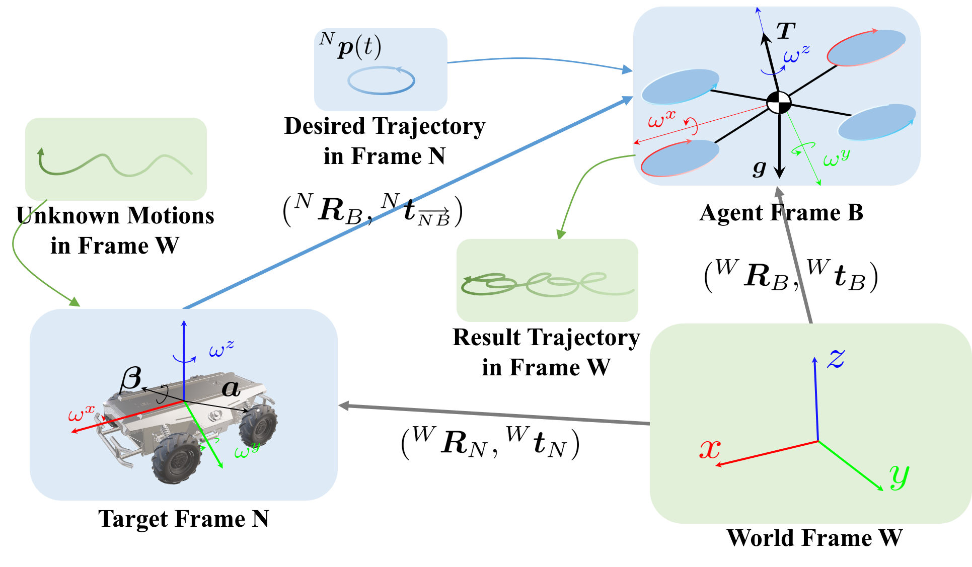
Figure 2: The transformation relationship among the quadrotor (the agent) body frame, the non-inertial (the target) frame, and the world frame. The target is controlled externally, and the agent is controlled by feeding reference (e.g. trajectory) defined in the target’s frame.

As shown in Fig. 2, we define the agent frame as $B$ attached to the body frame of the quadrotor, the target frame as $N$ attached to the body frame of the UGV, and frame $W$ is the inertial world frame. We denote scalar numbers with lowercase letters, vectors with bold lowercase letters, and matrices with bold uppercase letters. The left superscript indicates the coordinate system where the variable is expressed. If no other specification, values without any left superscript are expressed in the world frame $W$. For example, we denote the relative position of frame $B$ w.r.t. frame $N$ (non-inertial) by ${}^{N}\boldsymbol{p}_{B}$, the relative velocity by ${}^{N}\boldsymbol{v}_{B}$, and the relative orientation by ${}^{N}\boldsymbol{q}_{B}$. The right superscript $x$, $y$, or $z$ on a vector means the element of the vector, e.g., $\boldsymbol{t}^{x}$ is the $x$ element of $\boldsymbol{t}$. $\odot$ means quaternion Hamilton product. The skew-symmetric matrix of a vector $\boldsymbol{t}$ is denoted as $[\boldsymbol{t}]_{\times}$. The measured vector $\boldsymbol{v}$ from sensors is denoted as $\widehat{\boldsymbol{v}}$. Table I lists the main notations used in this paper.

TABLE I: Table of Notations

${}^{N}\boldsymbol{p}_{B}$	$\triangleq$	Relative position of the agent in the target’s frame
${}^{N}\boldsymbol{v}_{B}$	$\triangleq$	Relative velocity of the agent in the target’s frame
${}^{*}\boldsymbol{q}_{\#}$	$\triangleq$	Unit quaternion from $\#$ to $*$
${}^{*}\boldsymbol{R}_{\#}$	$\triangleq$	Rotation matrix from $\#$ to $*$
${}^{*}\boldsymbol{t}_{\scriptscriptstyle\overrightarrow{NB}}$	$\triangleq$	Translation vector from $N$ to $B$ expressed in $*$
$\boldsymbol{t}_{\#}$	$\triangleq$	Translation vector from $W$ to $\#$ expressed in $W$
$\boldsymbol{g}$	$\triangleq$	Gravitational acceleration
${}^{B}\boldsymbol{T}_{B}$	$\triangleq$	Normalized collective thrust of $B$, system input
${}^{B}\boldsymbol{\Omega}_{B}$	$\triangleq$	Body rate of $B$, system input
${}^{N}\boldsymbol{a}_{N}$	$\triangleq$	Linear acceleration of $N$ expressed in $N$
${}^{N}\boldsymbol{\Omega}_{N}$	$\triangleq$	Body rate (angular velocity) of $N$
${}^{N}\boldsymbol{\beta}_{N}$	$\triangleq$	Angular acceleration of $N$
$(r,v,\omega)$	$\triangleq$	Experiment parameter configuration

III-B Quadrotor System Model in Non-Inertial Frame

In this section, we derive the quadrotor system model in the non-inertial frame $N$ by introducing an intermediate inertial world frame $W$. Our derivation shows that all the dependencies on this world frame are eliminated at the end. Fig. 2 shows the relationship among the three frames. The relative position is:

$${}^{N}\boldsymbol{p}_{B}={}^{N}\boldsymbol{R}_{W}\boldsymbol{t}_{\scriptscriptstyle\overrightarrow{NB}}$$ (1)

where $\boldsymbol{t}_{\scriptscriptstyle\overrightarrow{NB}}=\boldsymbol{t}_{B}-\boldsymbol{t}_{N}$ is the translational vector pointing from the origin of frame $N$ to frame $B$. Then we get the relative velocity by applying a time derivative as following

$${}^{N}\dot{\boldsymbol{p}}_{B}={}^{N}\boldsymbol{v}_{B} =\frac{d}{dt}({}^{N}\boldsymbol{R}_{W})\boldsymbol{t}_{\scriptscriptstyle\overrightarrow{NB}}+{}^{N}\boldsymbol{R}_{W}\dot{\boldsymbol{t}}_{\scriptscriptstyle\overrightarrow{NB}}$$ (2)

$$=-[{}^{N}\boldsymbol{\Omega}_{N}]_{\times}{}^{N}\boldsymbol{R}_{W}\boldsymbol{t}_{\scriptscriptstyle\overrightarrow{NB}}+{}^{N}\boldsymbol{R}_{W}\dot{\boldsymbol{t}}_{\scriptscriptstyle\overrightarrow{NB}}$$

$$=-[{}^{N}\boldsymbol{\Omega}_{N}]_{\times}{}^{N}\boldsymbol{p}_{B}+{}^{N}\boldsymbol{R}_{W}\dot{\boldsymbol{t}}_{\scriptscriptstyle\overrightarrow{NB}}$$

The relative acceleration is the time derivative of the relative velocity

$${}^{N}\dot{\boldsymbol{v}}_{B} =-\frac{d}{dt}([{}^{N}\boldsymbol{\Omega}_{N}]_{\times}){}^{N}\boldsymbol{p}_{B}-[{}^{N}\boldsymbol{\Omega}_{N}]_{\times}{}^{N}\dot{\boldsymbol{p}}_{B}$$ (3)

$$-[{}^{N}\boldsymbol{\Omega}_{N}]_{\times}{}^{N}\boldsymbol{R}_{W}\dot{\boldsymbol{t}}_{\scriptscriptstyle\overrightarrow{NB}}+{}^{N}\boldsymbol{R}_{W}\ddot{\boldsymbol{t}}_{\scriptscriptstyle\overrightarrow{NB}}$$

$$=-\frac{d}{dt}([{}^{N}\boldsymbol{\Omega}_{N}]_{\times}){}^{N}\boldsymbol{p}_{B}-[{}^{N}\boldsymbol{\Omega}_{N}]_{\times}{}^{N}\boldsymbol{v}_{B}$$

$$-[{}^{N}\boldsymbol{\Omega}_{N}]_{\times}({}^{N}\boldsymbol{v}_{B}+[{}^{N}\boldsymbol{\Omega}_{N}]_{\times}{}^{N}\boldsymbol{p}_{B})+{}^{N}\boldsymbol{R}_{W}(\ddot{\boldsymbol{t}}_{B}-\ddot{\boldsymbol{t}}_{N})$$

$$=-[{}^{N}\boldsymbol{\beta}_{N}]_{\times}{}^{N}\boldsymbol{p}_{B}-2[{}^{N}\boldsymbol{\Omega}_{N}]_{\times}{}^{N}\boldsymbol{v}_{B}-[{}^{N}\boldsymbol{\Omega}_{N}]_{\times}^{2}{}^{N}\boldsymbol{p}_{B}$$

$$+{}^{N}\boldsymbol{R}_{B}{}^{B}\boldsymbol{T}_{B}+\underbrace{{}^{N}\boldsymbol{R}_{W}\boldsymbol{g}-{}^{N}\boldsymbol{R}_{W}\boldsymbol{a}_{N}}_{\text{values relying on estimations in }W}$$

where $\ddot{\boldsymbol{t}}_{B}$ in Equ. 3 is the acceleration of a quadrotor modeled in the world frame as a rigid body as in [21]

$$\ddot{\boldsymbol{t}}_{B}={}^{W}\boldsymbol{R}_{B}{}^{B}\boldsymbol{T}_{B}+\boldsymbol{g}$$ (4)

${}^{B}\boldsymbol{T}_{B}=[0,0,T]^{\top}$ is the normalized collective thrust of the quadrotor and $T=\sum_{i}T_{i},i\in\{1,2,3,4\}$ is the normalized thrust force from four motors, $\boldsymbol{g}=[0,0,-g]^{\top}$ is the gravity, ${}^{N}\boldsymbol{\Omega}_{N}$ is the body rate of the non-inertial frame, ${}^{N}\boldsymbol{\beta}_{N}$ is the angular acceleration of the non-inertial frame, ${}^{N}\boldsymbol{R}_{W}\boldsymbol{a}_{N}$ is the linear acceleration of the non-inertial frame expressed in the non-inertial frame.

The rotation matrix from $B$ to $N$ is

$${}^{N}\boldsymbol{R}_{B}={}^{N}\boldsymbol{R}_{W}{}^{W}\boldsymbol{R}_{B}$$ (5)

The time derivative of the above rotation matrix is

$${}^{N}\dot{\boldsymbol{R}}_{B} =\frac{d}{dt}({}^{N}\boldsymbol{R}_{W}){}^{W}\boldsymbol{R}_{B}+{}^{N}\boldsymbol{R}_{W}\frac{d}{dt}({}^{W}\boldsymbol{R}_{B})$$ (6)

$$=-[{}^{N}\boldsymbol{\Omega}_{N}]_{\times}{}^{N}\boldsymbol{R}_{B}+{}^{N}\boldsymbol{R}_{B}[{}^{B}\boldsymbol{\Omega}_{B}]_{\times}$$

At the same time, we show the quaternion here for model implementation in the next section

$${}^{N}\dot{\boldsymbol{q}}_{B} ={}^{N}\dot{\boldsymbol{q}}_{W}\odot{}^{W}\boldsymbol{q}_{B}+{}^{N}\boldsymbol{q}_{W}\odot{}^{W}\dot{\boldsymbol{q}}_{B}$$ (7)

$$=-\frac{1}{2}{}^{N}\boldsymbol{\Omega}_{N}\odot{}^{N}\boldsymbol{q}_{B}+\frac{1}{2}{}^{N}\boldsymbol{q}_{B}\odot{}^{B}\boldsymbol{\Omega}_{B}$$

In the system model of Equ. 3 and Equ. 7, we almost eliminate the dependency on values in world frame $W$ except for ${}^{N}\boldsymbol{R}_{W}$ in Equ. 3. We notice that the last two terms (${}^{N}\boldsymbol{R}_{W}\boldsymbol{g}-{}^{N}\boldsymbol{R}_{W}\boldsymbol{a}_{N}$) in Equ. 3 are actually the total measured acceleration of target expressed in target’s frame, which can be handled using the data from an IMU attached to the non-inertial frame to the relative system model directly. In detail, Equ. 3 contains the projected gravitational acceleration ${}^{N}\boldsymbol{R}_{W}\boldsymbol{g}$ and the acceleration of the non-inertial frame ${}^{N}\boldsymbol{a}_{N}$($={}^{N}\boldsymbol{R}_{W}\boldsymbol{a}_{N}$). The true acceleration of a MEMS IMU sensor can be calculated by applying the negative gravity in the target’s body frame as

$${}^{N}\boldsymbol{a}_{N}={}^{N}\boldsymbol{R}_{W}\prescript{W}{}{\begin{bmatrix}0\\ 0\\ -g\end{bmatrix}}+\prescript{N}{}{\begin{bmatrix}\hat{a}^{x}\\ \hat{a}^{y}\\ \hat{a}^{z}\end{bmatrix}}$$ (8)

where $\hat{a}^{x}$, $\hat{a}^{y}$, and $\hat{a}^{z}$ are the measured acceleration data from the IMU. With Equ. 8, Equ. 3 can be reformulated to

$${}^{N}\dot{\boldsymbol{v}}_{B} =-[{}^{N}\boldsymbol{\beta}_{N}]_{\times}{}^{N}\boldsymbol{p}_{B}-2[{}^{N}\widehat{\boldsymbol{\Omega}}_{N}]_{\times}{}^{N}\boldsymbol{v}_{B}-[{}^{N}\widehat{\boldsymbol{\Omega}}_{N}]_{\times}^{2}{}^{N}\boldsymbol{p}_{B}$$ (9)

$$+{}^{N}\boldsymbol{R}_{B}{}^{B}\boldsymbol{T}_{B}-{}^{N}\widehat{\boldsymbol{a}}_{N}$$

where ${}^{N}\widehat{\boldsymbol{a}}_{N}$ and ${}^{N}\widehat{\boldsymbol{\Omega}}_{N}$ are the measured linear acceleration and angular velocity from the IMU, respectively.

III-C CoNi-MPC

We propose a Cooperative Non-inertial Frame Based Model Predictive Control (CoNi-MPC) with the above system model targeting relative motion control. We define the cooperative system state $\boldsymbol{x}=[{}^{N}\boldsymbol{p}_{B};\;{}^{N}\boldsymbol{v}_{B};\;{}^{N}\boldsymbol{q}_{B};\;{}^{N}\widehat{\boldsymbol{a}}_{N};\;{}^{N}\widehat{\boldsymbol{\Omega}}_{N};\;{}^{N}\boldsymbol{\beta}_{N}]\in\mathbb{R}^{19}$. The first three vectors ${}^{N}\boldsymbol{p}_{B}$, ${}^{N}\boldsymbol{v}_{B}$, and ${}^{N}\boldsymbol{q}_{B}$, as defined in above section, are the relative quantities in the system. The last three vectors ${}^{N}\widehat{\boldsymbol{a}}_{N}$, ${}^{N}\widehat{\boldsymbol{\Omega}}_{N}$, and ${}^{N}\boldsymbol{\beta}_{N}$ contain the dynamic information of the non-inertial frame. The time derivative of the angular velocity is $\frac{d}{dt}({}^{N}\widehat{\boldsymbol{\Omega}}_{N})={}^{N}\boldsymbol{\beta}_{N}$. For the linear and angular accelerations, we assume their change rates are 0 in each control window, i.e., ${}^{N}\dot{\widehat{\boldsymbol{a}}}_{N}=0$ and $\dot{\boldsymbol{\beta}}_{N}=0$. As they are relatively high order values, this assumption does not affect the performance very much for our system. We put the dynamic information of the non-inertial frame in the state vector for convenience in the implementation part and for future improvement on a actively collaborative system (expanding the control vector and adding the dynamic evolution of frame $N$). The control input is $\boldsymbol{u}=[T;\;{}^{B}\Omega_{B}^{x};\;{}^{B}\Omega_{B}^{y};\;{}^{B}\Omega_{B}^{z}]\in\mathbb{R}^{4}$ where $T=\sum_{i=1}^{4}T_{i}$.

We define the quadratic cost

$$\boldsymbol{C}(\boldsymbol{x},\boldsymbol{u})=\lVert\boldsymbol{x}(t)-\boldsymbol{x}(t)_{ref}\rVert_{\boldsymbol{Q}}+\lVert\boldsymbol{u}(t)-\boldsymbol{u}_{h}\rVert_{\boldsymbol{R}}$$

where $\lVert\boldsymbol{x}\rVert_{\boldsymbol{M}}=\boldsymbol{x}^{\top}\boldsymbol{M}\boldsymbol{x}$ and $\boldsymbol{u}_{h}=[g;0;0;0]$ is the hover input. The discretized optimization problem is

$$\min_{\boldsymbol{u}_{0},\dots,\boldsymbol{u}_{N-1}} \sum_{k=0}^{N-1}(\lVert\boldsymbol{x}(k)-\boldsymbol{x}(k)_{ref}\rVert_{\boldsymbol{Q}}+\lVert\boldsymbol{u}(k)-\boldsymbol{u}_{h}\rVert_{\boldsymbol{R}})$$ (10)

$$+\lVert\boldsymbol{x}(N)-\boldsymbol{x}(N)_{ref}\rVert_{\boldsymbol{Q}_{final}}$$

s.t. $$\boldsymbol{x}(0)=\boldsymbol{x}_{0}$$

$$\boldsymbol{x}(k+1)=f_{d}(\boldsymbol{x}(k),\boldsymbol{u}(k))$$

$$T_{\text{min}}\leq T\leq T_{\text{max}}$$

$$\lVert{}^{B}\Omega_{B}^{x}\rVert\leq\Omega_{\text{rp}}$$

$$\lVert{}^{B}\Omega_{B}^{y}\rVert\leq\Omega_{\text{rp}}$$

$$\lVert{}^{B}\Omega_{B}^{z}\rVert\leq\Omega_{\text{yaw}}$$

where $\boldsymbol{x}_{0}$ is the state estimation of the system in each control iteration, $f_{d}$ is the discretized system model, $T_{\text{min}}$ is the minimum thrust, $T_{\text{max}}$ is the maximum thrust constraint, $\Omega_{\text{rp}}$ is the maximum roll and pitch angular speed, and $\Omega_{\text{yaw}}$ is the maximum yaw angular speed.

As our system does not rely on any information in the global world frame and only relates to the agent and target, the system can handle the cooperation between robots elegantly. Tasks like leader-follower, landing, orbit flight, rings crossing, etc. can be solved by simply defining the reference in the CoNi-MPC. The advantage of the system is that the reference is fixed, which is just a pre-computed expression of the relative motion between robots and does not need any online replaning. We classify the reference into two categories, fixed-point scheme and fixed-plan scheme, corresponding to leader-follower and complex motion respectively.

III-C1 Fixed point scheme (leader and follower)

The proposed method can be easily used for leader-follower control. CoNi-MPC only needs a fixed point (containing the full state) so as to let the agent track that point while the target moves. For example, an array containing the same point reference, $\boldsymbol{x}(k)=[(0,0,z),\boldsymbol{0}^{\top},(1,0,0,0),\boldsymbol{0}^{\top},\boldsymbol{0}^{\top},\boldsymbol{0}^{\top}]^{\top}$, fed to the controller will let the agent hover at the ${}^{N}\boldsymbol{p}_{B}=(0,0,z)^{\top}$ point in the non-inertial target frame with the same orientation of the target frame, even if the target frame may arbitrarily move in the world frame.

III-C2 Fixed plan scheme (complex trajectories)

For complex tasks such as landing, orbit flight, and rings crossing, we simply need to define the trajectory of the agent in the target frame. The landing tasks can use a trajectory approaching the origin of $N$ frame and the orbit flight is a circle trajectory directly. We adopt our previous work of a minimum control effort polynomial trajectory class named MINCO [22] to define the relative trajectory between robot. MINCO trajectory can achieve smooth motions by decoupling the space and time parameters of the trajectory for users, which greatly improves the quality and efficiency of trajectory generation. We only need to take initial and terminal relative states of the UAV as boundary conditions, and specify the position of intermediate waypoints and the time duration of each piece to obtain a polynomial trajectory $\boldsymbol{p}({t})$ with minimum jerk. Furthermore, we limit the maximum relative velocity and acceleration to guarantee dynamic feasibility. After discretizing $\boldsymbol{p}({t})$ and calculating the orientation based on the differential flatness of multicopters [23], we can get a series of reference states $\{[{}^{N}\boldsymbol{p}_{B}(k)\;;{}^{N}\boldsymbol{v}_{B}(k)\;;{}^{N}\boldsymbol{q}_{B}(k)]\}_{k=0}^{N}$. Thus, the proposed controller can be fed with only one fixed global trajectory to achieve autonomous landing and tracking while the UGV moves.

III-D Implementation

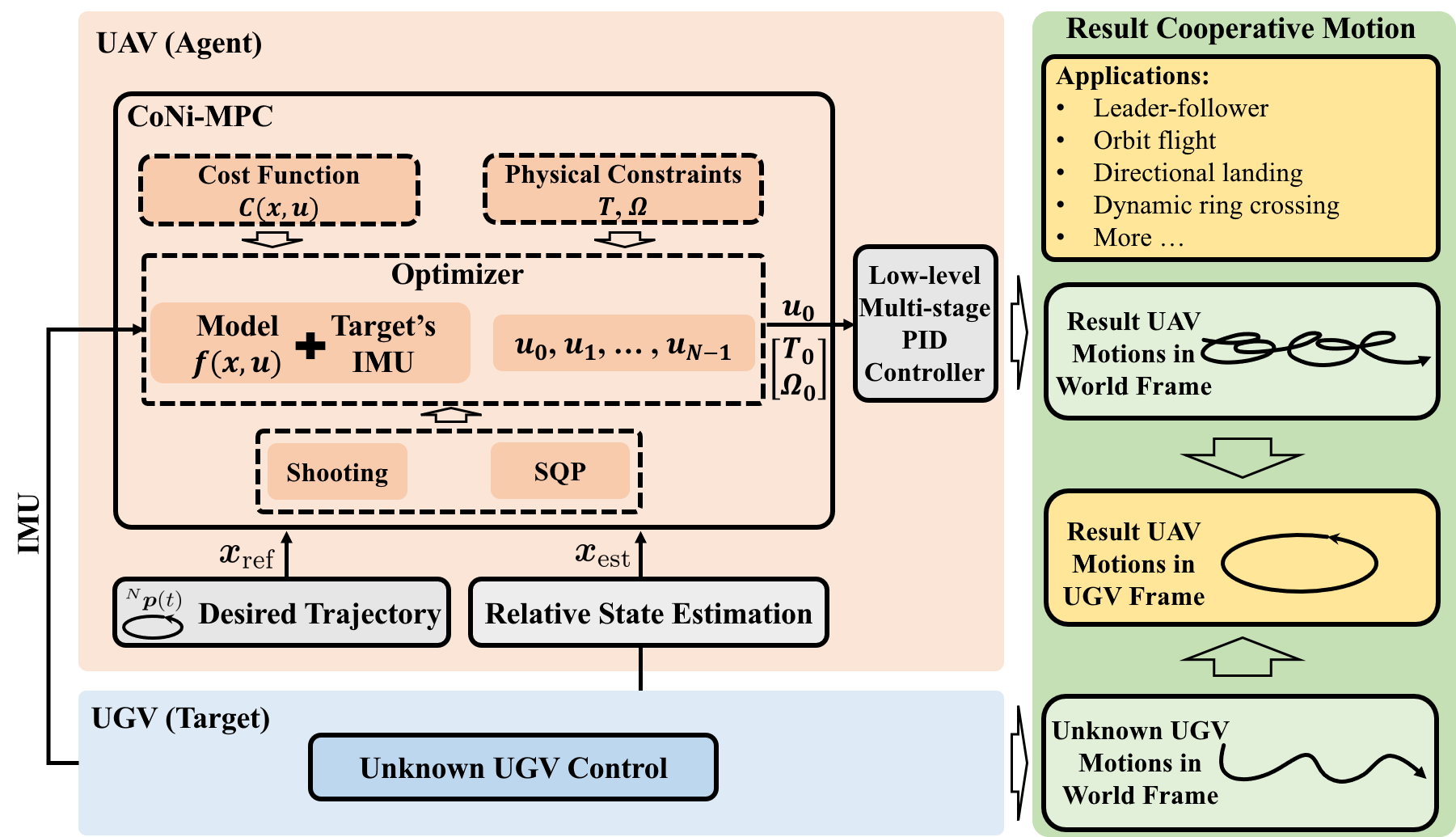
Figure 3: System overview and implementation of UAV-UGV cooperative motion control using CoNi-MPC.

Fig. 3 shows the system overview of UAV-UGV cooperative motion control system. A CoNi-MPC controller, implemented using ACADO toolkit [24], is employed by the UAV and works as a high-level controller to produce thrust and body rate control command $\boldsymbol{u}_{0}$. A low-level multi-stage PID controllers is used to track the control command. CoNi-MPC needs a pre-defined desired relative motion trajectory refer to the UGV as motion control target. With input of UGV’s IMU measurements and relative state estimations, CoNi-MPC solves a optimization via multiple shooting technique and Runge-Kutta integration scheme. An average signal filter is applied to the IMU data from the non-inertial frame, which is transmitted through ROS’s multi-machine communication mechanism in current setup. The relative estimation can be generated either from a motion capture system or directly from our previous work of CREPES [25], a relative estimation device. For each control iteration of the MPC optimization problem, we set the time window as $T=2$ seconds and discretization time step $dt=0.1$ second. The real control loop time of the MPC is around 10 ms, which is smaller than $dt=100$ ms. This implementation differs from standard MPC formulation, where CoNi-MPC uses latest relative state to produce the control command much more frequently, but with relatively small scale optimization problem to save computation cost. In each iteration, the initial state is set as the current estimated relative state $\boldsymbol{x}_{\text{est}}$. For ${}^{N}\widehat{\boldsymbol{a}}_{N}$, ${}^{N}\widehat{\boldsymbol{\Omega}}_{N}$, and ${}^{N}\boldsymbol{\beta}_{N}$, the penalty terms for them are set to $\boldsymbol{Q}(i,i)=0,\;\forall i=10\dots 19$. Note that in the simulation and experiment, since the angular acceleration is hard to retrieve, we set this term to $\boldsymbol{0}$ both in estimations and references, which assumes that the non-inertial frame rotates with a constant angular velocity in each prediction horizon.

IV Experiments

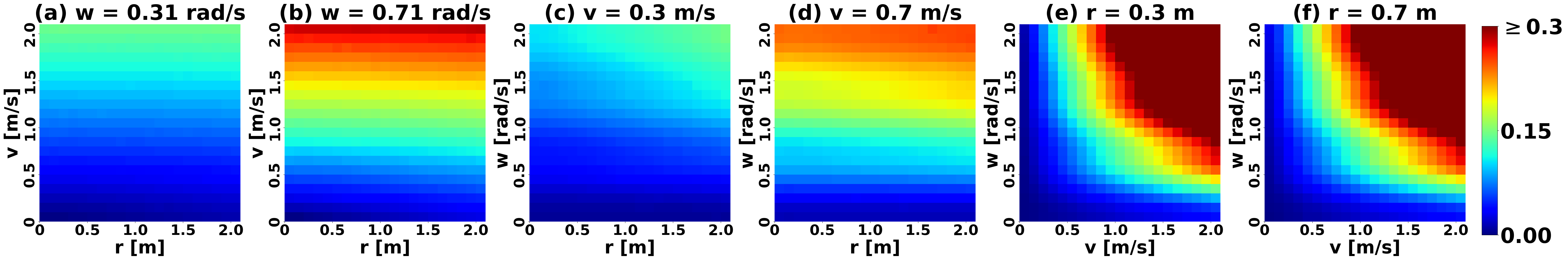
Figure 4: Mean errors for tracking a point with different $(r,v,\omega)$ settings. (a-b) error distribution of $r-v$ with $\omega=$ 0.31 and 0.71. (c-d) error distribution of $\omega-r$ with $v=$ 0.3 and 0.7. (e-f) error distribution of $\omega-v$ with $r=$ 0.3 and 0.7.

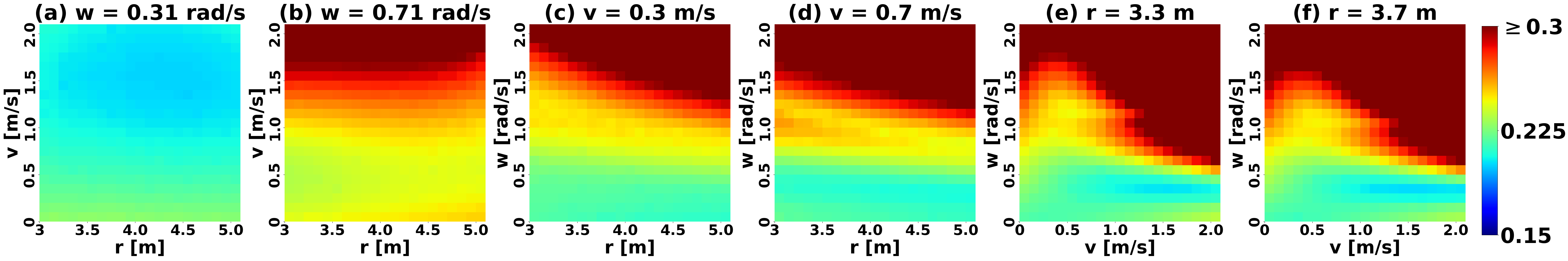
Figure 5: Mean errors for tracking a landing trajectory with different $(r,v,\omega)$ settings. (a-b) error distribution of $r-v$ with $\omega=$ 0.31 and 0.71. (c-d) error distribution of $\omega-r$ with $v=$ 0.3 and 0.7. (e-f) error distribution of $\omega-v$ with $r=$ 3.3 and 3.7.

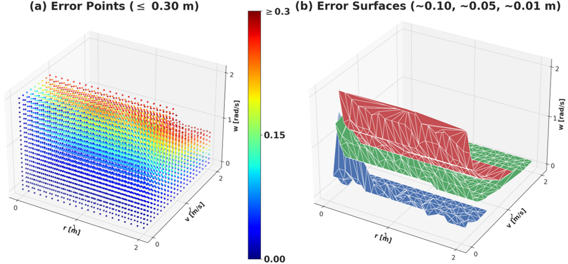
Figure 6: Mean errors for tracking a point with different $(r,v,\omega)$ settings. (a) illustrates the data points with tracking error $\leq$ 0.30 m. (b) shows three surfaces of data points with around tracking errors of 0.10 (red), 0.05 (green), and 0.01 (blue) m.

Consider a UAV-UGV cooperative system, the uncontrolled motions of the UGV place a crucial role for the system performance. Most results of UAV-UGV cooperative tasks, such as the autonomous landing in [6] and [9], only show the UGV with constant linear velocities without any aggressive rotational movements. However, whether that UAV can track the UGV with both aggressive linear and angular motions well is the key point to consider when applying this system to corresponding tasks. From Equ. 9 it can be inferred that ${}^{N}\boldsymbol{p}_{B}$, ${}^{N}\widehat{\boldsymbol{\Omega}}_{N}$, ${}^{N}\boldsymbol{\beta}_{N}$, and ${}^{N}\widehat{\boldsymbol{a}}_{N}$ affect the relative acceleration ${}^{N}\dot{\boldsymbol{v}}_{B}$. Meanwhile, ${}^{N}\boldsymbol{\Omega}_{N}$, ${}^{N}\boldsymbol{p}_{B}$, and the relative linear velocity in $W$, $\dot{\boldsymbol{t}}_{\scriptscriptstyle\overrightarrow{NB}}$, are coupled in the relative velocity (Equ. 2). In order to test the performance of the proposed controller, we decouple the variables and pick the parameters $(r,v,\omega)$ to conduct parameter study. These parameters stand for the range (x-y plane) between robots, linear and angular velocity of the target, which also fits the cooperative task intuitively. Parameters definition and theoretical analysis is as following.

• $r\triangleq-{}^{N}\boldsymbol{p}_{B}^{x}$, s.t. ${}^{N}\boldsymbol{p}_{B}^{x}<0$, ${}^{N}\boldsymbol{p}_{B}^{y}=0$, ${}^{N}\boldsymbol{p}_{B}^{z}=z(t)\geq 0$ where $z(t)$ can be fixed or time-varying

• $v\triangleq({}^{N}\boldsymbol{R}_{W}\dot{\boldsymbol{t}}_{N})^{x}$, s.t. $({}^{N}\boldsymbol{R}_{W}\dot{\boldsymbol{t}}_{N})^{x}>0$, $({}^{N}\boldsymbol{R}_{W}\dot{\boldsymbol{t}}_{N})^{y}=0$, $({}^{N}\boldsymbol{R}_{W}\dot{\boldsymbol{t}}_{N})^{z}=0$

• $\omega\triangleq{}^{N}\boldsymbol{\Omega}_{N}^{z}$, s.t. ${}^{N}\boldsymbol{\Omega}_{N}^{x}=0$, ${}^{N}\boldsymbol{\Omega}_{N}^{y}=0$, ${}^{N}\boldsymbol{\Omega}_{N}^{z}>0$

For simplicity, if no other specification, the units of the configuration $(r,v,\omega)$ are m, m/s, and rad/s by default, respectively. We expand Equ. 2 and 9 in three dimensions to show how $(r,v,\omega)$ are involved in the system model:

$${}^{N}{\boldsymbol{{v}}}_{B}^{x} =({}^{N}\boldsymbol{R}_{W}\dot{\boldsymbol{t}}_{B})^{x}-v$$ (11)

$${}^{N}{\boldsymbol{{v}}}_{B}^{y} =({}^{N}\boldsymbol{R}_{W}\dot{\boldsymbol{t}}_{B})^{y}-wr$$

$${}^{N}{\boldsymbol{{v}}}_{B}^{z} =({}^{N}\boldsymbol{R}_{W}\dot{\boldsymbol{t}}_{B})^{z}$$

$${}^{N}\dot{\boldsymbol{{v}}}_{B}^{x} =2\omega({}^{N}\boldsymbol{R}_{W}\dot{\boldsymbol{t}}_{B})^{y}+({}^{N}\boldsymbol{R}_{B}{}^{B}\boldsymbol{T}_{B})^{x}-({}^{N}\widehat{\boldsymbol{a}}_{N})^{x}$$

$${}^{N}\dot{\boldsymbol{{v}}}_{B}^{y} =-2\omega({}^{N}\boldsymbol{R}_{W}\dot{\boldsymbol{t}}_{B})^{x}+2\omega v+({}^{N}\boldsymbol{R}_{B}{}^{B}\boldsymbol{T}_{B})^{y}-({}^{N}\widehat{\boldsymbol{a}}_{N})^{y}$$

$${}^{N}\dot{\boldsymbol{{v}}}_{B}^{z} =({}^{N}\boldsymbol{R}_{B}{}^{B}\boldsymbol{T}_{B})^{z}-9.8$$

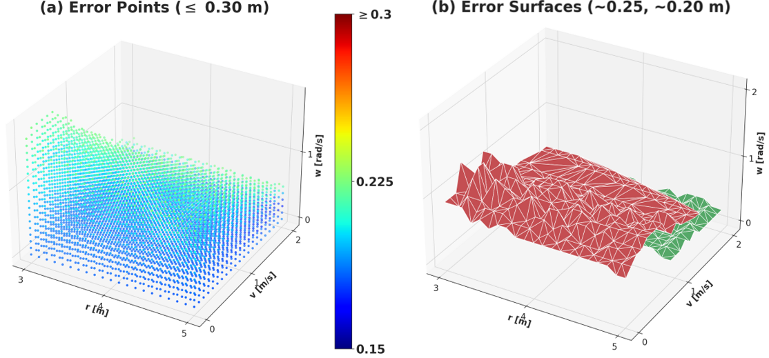
Figure 7: Mean errors for tracking a landing trajectory with different $(r,v,\omega)$ settings. (a) illustrates the data points with tracking error $\leq$ 0.30 m. (b) shows three surfaces of data points with around tracking errors of 0.25 (red) and 0.20 (green) m.

In the experiment, apart from the range parameter, the target UGV is programmed with a circular motion with different $v,w$ combination in the world frame (the radius of circle is $v/\omega$). We classify the experiments into two schemes, fixed point and fixed plan scheme. The first is to control the quadrotor follow a fixed point (e.g., ${}^{N}{\boldsymbol{{p}}}_{B}=(-r,0,z)^{\top}$) in the non-inertial frame. We set the $z$ as 2.0 m in simulation and 1.0 m in real experiment. For example, the configuration $(r,v,\omega)=(\underline{1.0\text{ m}},\underline{1.0\text{ m/s}},\underline{0.5\text{ rad/s}})$ represents the quadrotor will follow a fixed point $(\underline{-1.0\text{ m}},0.0\text{ m},2.0\text{ m})$ in the non-inertial frame with forward 1.0 m/s speed and counter-clockwise 0.5 rad/s rotating speed. The other test scheme is fixed plan experiment. The configuration has same meaning with the $(v,w)$ but the $r$ stands for the inertial range of the fixed landing trajectory. The quadrotor will follow the pre-computed trajectory to land at the origin of the non-inertial frame. For example, $\underline{r=1.0}$ represents that the landing trajectory will start at ${}^{N}{\boldsymbol{{p}}}_{B}=(\underline{-1.0},0.0,2.0)^{\top}$ and end at ${}^{N}{\boldsymbol{{p}}}_{B}=(0,0,0)^{\top}$. For each scheme, we define the tracking error $e_{i}$ at each control iteration $i$ as $e_{i}=\lVert({}^{N}\boldsymbol{p}_{B})_{\text{est}}-({}^{N}\boldsymbol{p}_{B})_{\text{ref},i}(0)\rVert$ which is the distance that the the current estimated point deviates from the first point of the reference window. The mean tracking error for each scheme is defined as $\bar{e}=\sum_{i}e_{i}/M$, where $M$ is the total number of iterations.

IV-A Simulation

The numerical simulation is performed on a work station with an AMD Ryzen PRO 5995WX CPU, where we use 64 Docker containers simultaneously simulating the quadrotor system model with different parameter configurations using the proposed controller. The MPC in the simulation runs over 100Hz. For all simulations, the range of the control inputs is set to

• $T\in[2.0,20.0]\;\text{m}/\text{s}^{2}$

• ${}^{B}\boldsymbol{\Omega}_{B}^{i}\in[-3.14,3.14]$ rad/s $\forall i\in\{x,y,z\}$

The penalty matrices $\boldsymbol{Q}$ and $\boldsymbol{R}$ and the constraints are the same. The simulated relative estimation is added with a Gaussian noise to represent real sensors, where $\boldsymbol{\sigma}({{}^{N}\boldsymbol{p}_{B}})^{i}=0.025\;\text{m}$, $\boldsymbol{\sigma}({{}^{N}\boldsymbol{v}_{B}})^{i}=0.025\;\text{m}/\text{s}$, $\boldsymbol{\sigma}({\theta({}^{N}\boldsymbol{q}_{B})})^{i}=0.044\;\text{rad}$ ($5^{\circ}$, $\theta(\cdot)$ is the rotation angle of the quaternion along the rotation axis), $\boldsymbol{\sigma}({{}^{N}\widehat{\boldsymbol{a}}_{N}})^{i}=0.025\;\text{m}/\text{s}^{2}$, and $\boldsymbol{\sigma}({{}^{N}\boldsymbol{\Omega}_{N}})^{i}=0.044\;\text{rad}/\text{s}$ ($5^{\circ}/s$), where $i\in\{x,y,z\}$.

The parameter configurations of the fixed-point scheme are set with $r\in[0.0,2,0]$, $v\in[0.0,2.0]$, and $\omega\in[0.01,2.01]$ all with stepsizes of $0.1$. Fig. 4 illustrates the tracking errors for different $r,v,\omega$ combinations by selecting two example values for each parameter. The parameters for the fixed-plan scheme are: $r\in[3.0,5.0]$, $v\in[0.0,2.0]$, and $\omega\in[0.01,2.01]$ all with stepsizes of $0.1$. Fig. 5 illustrates the mean tracking errors with the same logic. We consider tracking error more than 0.30 m as tracking failure and they are shown in the dark red regions in Fig. 4 and 5. In Fig. 6 and 7, we show all the errors in 3D in the left and selected error surfaces (relation between result error and $r,v,\omega$) in the right. From these figures, we can conclude that the angular velocity $\omega$ of the non-inertial frame affects the tracking error most. For a fixed $\omega$, the tracking error increases as $v$ grows. For a landing task, the simulations can help find the safe $(r,v,\omega)$ parameters that can guarantee the success of landing.

IV-B Real-World Experiment

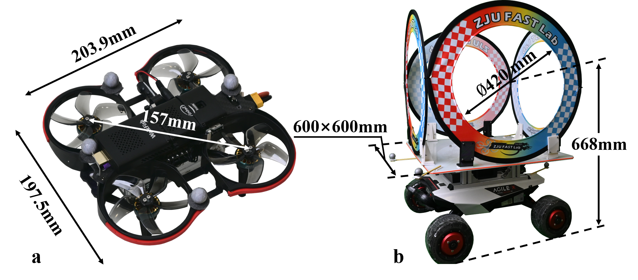
Figure 8: The quadrotor and UGV in our real experiments.

We have conducted both indoor and outdoor experiments to verify our system. The relative estimation can be generated directly from CREPES[25] or computed from NOKOV motion capture system for outdoor or indoor experiments respectively. Fig. 8 shows the UAV and UGV platform and their dimensions. The quadrotor weighs 591.8g and has a thrust-to-weight ratio of 2.03. The CoNi-MPC of UAV runs on a onboard computer with an Intel Celeron J4125 processor (2 to 2.7 GHz) and 8GB RAM. The proposed CoNi-MPC has computation time (one iteration) of 4.58 ms on average with standard deviation of 1.2 ms, which runs over 100Hz on the onboard computer.

According to the numerical simulation results, we select several representative parameters for both the fixed point and fixed plan schemes. The constraints in the MPC formulation are the same as that in the simulation. The parameters and the corresponding average tracking errors of both schemes are listed in Table II, We plot the tracking performance alone with time of two tests in details in Fig. 9 and 10.

Fig. 11 shows an qualitative result of a more demanding task, dynamic multi-ring crossing experiment. By simply apply a pre-computed 8-shape trajectory to CoNi-MPC, the quadrotor can continuously cross four rings attached to the four sides of a UGV while the UGV moves along an S-shape trajectory in the world frame. The diameter of rings for the UAV to cross is only two times of the UAV’s width, about 100 mm free at each side. Based on CREPES [25], we also performed outdoor experiments where the UGV is controlled arbitrarily and the UAV follows a circle trajectory. Please note there is no GPS/SLAM/anchors technology used to realize this task. Fig. 12 shows the tracking snapshots.

TABLE II: Average Tracking Errors of Real Experiments

Fixed point		Fixed plan
$(r,v,\omega)$	Error [m]	$(r,v,\omega)$	Error [m]
$(1.0,1.0,0.31)$	0.13	${(\textbf{4.0},\textbf{1.0},\textbf{0.31})}$	0.15
$(1.0,1.0,0.71)$	0.23	$(4.0,1.0,0.71)$	0.19
$(1.0,0.3,1.0)$	0.13	$(4.0,0.3,1.0)$	0.21
$(1.0,0.7,1.0)$	0.14	$(4.0,0.7,1.0)$	0.24
${(\textbf{0.3},\textbf{1.0},\textbf{1.0})}$	0.11	$(3.3,1.0,1.0)$	0.18
$(0.7,1.0,1.0)$	0.16	$(3.7,1.0,1.0)$	0.23

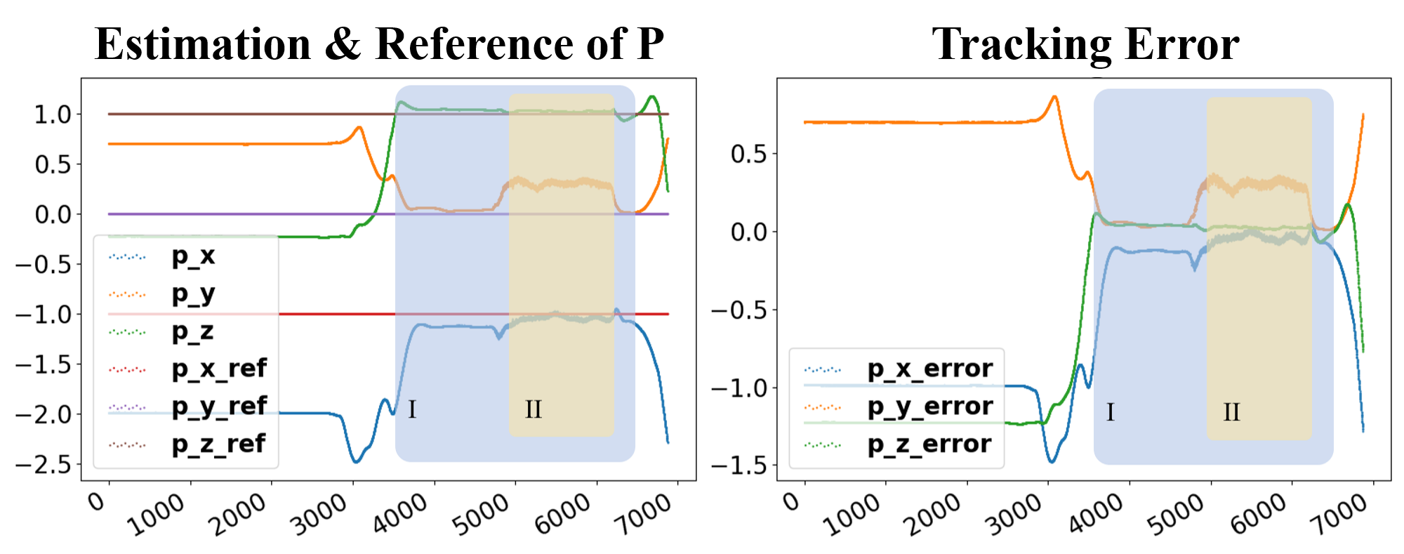
Figure 9: Fixed point experiment with $(1.0,1.0,0.71)$ setting. Blue (I) is for off-board mode; orange (II) is for UGV moving.

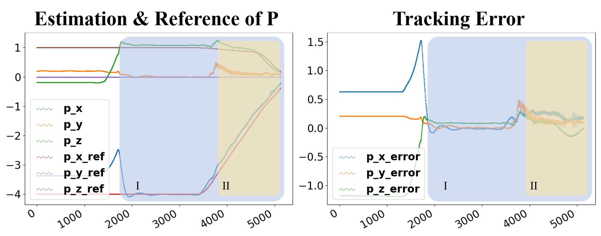
Figure 10: Fixed plan experiment with $(4.0,1.0,0.71)$ setting. Blue (I) is for off-board mode; orange (II) is for UGV moving.

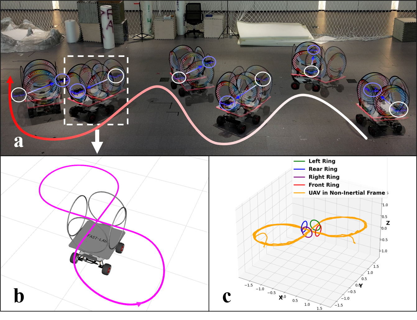
Figure 11: Rings crossing experiment. The UGV moves with an average speed of 0.15 m/s and a maximal speed of 0.38 m/s while the UAV can cross the ring attached to it.

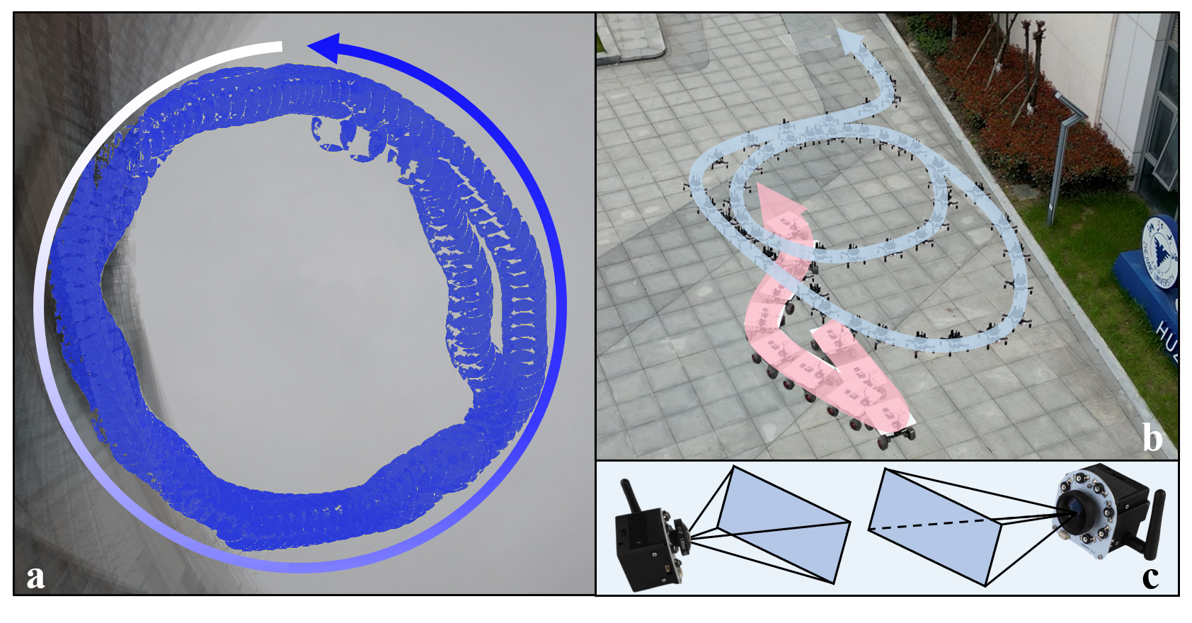
Figure 12: Outdoor experiment. (a) is shot from the camera on the UGV, and (b) is shot from third-person view. The UAV follows a circular trajectory while the UGV arbitrarily moves. (c) shows CREPES devices we use in the outdoor experiment.

V Conclusion

In this work, we present a thorough relative system dynamic model for a quadrotor in a non-inertial frame with linear and angular motions. Based on this model, we design and implement CoNi-MPC targeting cooperative UAV-UGV cooperation tasks, by taking the UGV as a non-inertial frame. Unlike traditional methods, this method bypasses the dependency of global state estimation of the agent and/or the target in the world frame. The system also avoids relying on prior knowledge of the target and does not need complex trajectory re-planning. CoNi-MPC only requires the relative states (pose and velocity), the angular velocity and the accelerations of the target, which can be obtained by relative localization methods and ubiquitous MEMS IMU sensors, respectively. We have performed extensive fixed-point and fixed-plan simulations and considerable real world experiments to test the proposed system. Experiment results show that the controller has promising robustness and tracking performance. For future works, this method can be extended to achieve multi-agent formation control and more demanding cooperative tasks.

References

- [1] T. Miki, P. Khrapchenkov, and K. Hori, “Uav/ugv autonomous cooperation: Uav assists ugv to climb a cliff by attaching a tether,” in International Conference on Robotics and Automation (ICRA). IEEE, 2019, pp. 8041–8047.
- [2] G. A. Di Caro and A. W. Z. Yousaf, “Multi-robot informative path planning using a leader-follower architecture,” in IEEE International Conference on Robotics and Automation (ICRA). IEEE, 2021, pp. 10 045–10 051.
- [3] L. Quan, L. Yin, T. Zhang, M. Wang, R. Wang, S. Zhong, Y. Cao, C. Xu, and F. Gao, “Formation flight in dense environments,” arXiv preprint arXiv:2210.04048, 2022.
- [4] M. Demirhan and C. Premachandra, “Development of an automated camera-based drone landing system,” IEEE Access, vol. 8, pp. 202 111–202 121, 2020.
- [5] P. Vlantis, P. Marantos, C. P. Bechlioulis, and K. J. Kyriakopoulos, “Quadrotor landing on an inclined platform of a moving ground vehicle,” in IEEE International Conference on Robotics and Automation (ICRA). IEEE, 2015, pp. 2202–2207.
- [6] G. Niu, Q. Yang, Y. Gao, and M.-O. Pun, “Vision-based autonomous landing for unmanned aerial and ground vehicles cooperative systems,” IEEE robotics and automation letters, vol. 7, no. 3, pp. 6234–6241, 2021.
- [7] Z. Han, R. Zhang, N. Pan, C. Xu, and F. Gao, “Fast-tracker: A robust aerial system for tracking agile target in cluttered environments,” in IEEE International Conference on Robotics and Automation (ICRA). IEEE, 2021, pp. 328–334.
- [8] J. Ji, T. Yang, C. Xu, and F. Gao, “Real-time trajectory planning for aerial perching,” in IEEE/RSJ International Conference on Intelligent Robots and Systems (IROS). IEEE, 2022, pp. 10 516–10 522.
- [9] P. Wang, C. Wang, J. Wang, and M. Q.-H. Meng, “Quadrotor autonomous landing on moving platform,” arXiv preprint arXiv:2208.05201, 2022.
- [10] Z. Han, K. Guo, L. Xie, and Z. Lin, “Integrated relative localization and leader–follower formation control,” IEEE Transactions on Automatic Control, vol. 64, no. 1, pp. 20–34, 2018.
- [11] J. I. Giribet, L. J. Colombo, P. Moreno, I. Mas, and D. V. Dimarogonas, “Dual quaternion cluster-space formation control,” IEEE Robotics and Automation Letters, vol. 6, no. 4, pp. 6789–6796, 2021.
- [12] D. Falanga, P. Foehn, P. Lu, and D. Scaramuzza, “Pampc: Perception-aware model predictive control for quadrotors,” in IEEE/RSJ International Conference on Intelligent Robots and Systems (IROS). IEEE, 2018, pp. 1–8.
- [13] L. Sun and W. Huo, “6-dof integrated adaptive backstepping control for spacecraft proximity operations,” IEEE Transactions on Aerospace and Electronic Systems, vol. 51, no. 3, pp. 2433–2443, 2015.
- [14] Y. Marani, K. Telegenov, E. Feron, and M.-T. L. Kirati, “Drone reference tracking in a non-inertial frame: control, design and experiment,” in IEEE/AIAA 41st Digital Avionics Systems Conference (DASC). IEEE, 2022, pp. 1–8.
- [15] C. Jin, M. Zhu, L. Sun, and Z. Zheng, “Relative motion modeling and control for a quadrotor landing on an unmanned vessel,” in AIAA Guidance, Navigation, and Control Conference, 2017, p. 1522.
- [16] Y. Li, G. Lu, D. He, and F. Zhang, “Robocentric model-based visual servoing for quadrotor flights,” IEEE/ASME Transactions on Mechatronics, 2023.
- [17] L. DeVries and J. Dawkins, “Multi-vehicle target tracking and formation control in non-inertial reference frames,” Annual American Control Conference (ACC), 4026-4031, 2018.
- [18] J. Ji, X. Zhou, C. Xu, and F. Gao, “Cmpcc: Corridor-based model predictive contouring control for aggressive drone flight,” in Experimental Robotics: The 17th International Symposium. Springer, 2021, pp. 37–46.
- [19] A. Romero, S. Sun, P. Foehn, and D. Scaramuzza, “Model predictive contouring control for time-optimal quadrotor flight,” IEEE Transactions on Robotics, vol. 38, no. 6, pp. 3340–3356, 2022.
- [20] T. P. d. Nascimento, G. F. Basso, C. E. T. Dórea, and L. M. G. Gonçalves, “Perception-driven motion control based on stochastic nonlinear model predictive controllers,” IEEE/ASME Transactions on Mechatronics, vol. 24, no. 4, pp. 1751–1762, 2019.
- [21] M. W. Mueller, M. Hehn, and R. D’Andrea, “A computationally efficient motion primitive for quadrocopter trajectory generation,” IEEE transactions on robotics, vol. 31, no. 6, pp. 1294–1310, 2015.
- [22] Z. Wang, X. Zhou, C. Xu, and F. Gao, “Geometrically constrained trajectory optimization for multicopters,” IEEE Transactions on Robotics, vol. 38, no. 5, pp. 3259–3278, 2022.
- [23] D. Mellinger and V. Kumar, “Minimum snap trajectory generation and control for quadrotors,” in IEEE international conference on robotics and automation. IEEE, 2011, pp. 2520–2525.
- [24] B. Houska, H. J. Ferreau, and M. Diehl, “Acado toolkit—an open-source framework for automatic control and dynamic optimization,” Optimal Control Applications and Methods, vol. 32, no. 3, pp. 298–312, 2011.
- [25] Z. Xun, J. Huang, Z. Li, C. Xu, F. Gao, and Y. Cao, “Crepes: Cooperative relative pose estimation towards real-world multi-robot systems,” arXiv preprint arXiv:2302.01036, 2023.