Geometry of quasiperiodic functions on the plane

Abstract.

The present article proposes a review of the most recent results obtained in the study of Novikov’s problem on the description of the geometry of the level lines of quasi-periodic functions in the plane. Most of the paper is devoted to the results obtained for functions with three quasi-periods, which play a very important role in the theory of transport phenomena in metals. In this part, along with previously known results, a number of new results are presented that significantly refine the general description of the picture that arises in this case. New statements are also presented for the case of functions with more than three quasi-periods, which open up approaches to the further study of Novikov’s problem in the most general formulation. The role of Novikov’s problem in various fields of mathematical and theoretical physics is also discussed.

1. Introduction

The theory of quasi-periodic functions originates in the works of G. Bohr and A.S. Besikovich ([1, 2]) and plays an important role in the description of a huge variety of phenomena in various fields of theoretical and applied science. As a rule, a quasi-periodic function $f(x^{1},\dots,x^{n})$ with $N$ quasi-periods in the space $\mathbb{R}^{n}$ is the restriction of a “good enough” (for example, smooth) $N$-periodic function $F(z^{1},\dots,z^{N})$ onto the image of the space $\mathbb{R}^{n}$ under some affine embedding $\iota:\mathbb{R}^{n}\hookrightarrow\mathbb{R}^{N}$, i.e. $f=F\circ\iota$. In the case of a generic embedding $\iota$, the function $f(x^{1},\dots,x^{n})$ has no exact periods in $\mathbb{R}^{n}$. Such periods appear when the intersection of the subspace $\iota(\mathbb{R}^{n})$ with the lattice $\mathbb{Z}^{N}$ is not empty. It may also turn out that the image $\iota(\mathbb{R}^{n})$ is contained in a non-trivial subspace of an integral direction. In this case, the number of quasi-periods of the function $f$ will be less than $N$.

In this paper, both the generic cases and special cases of quasi-periodic functions corresponding to embeddings $\iota:\mathbb{R}^{n}\hookrightarrow\mathbb{R}^{N}$ of various types will be important for us.

It is well known that the theory of quasiperiodic functions is extremely important in the description of quasicrystals. In this case, the physically important cases are $n=2$ and $n=3$, and $N$ is most often equal to $2n$. In addition, the theory of quasi-periodic functions underlies the description of solutions to integrable dynamical systems (both finite- and infinite-dimensional).

In this survey, we consider qualitative questions of the geometry of quasiperiodic functions on the plane. By this we mean the global behavior of their level lines $f(x,y)={\rm const}$, which plays a very important role in the description of a large number of physical phenomena. The problem of a qualitative description of the geometry of the level lines of quasi-periodic functions on the plane (Novikov’s problem) is very non-trivial, and its complexity grows rapidly with an increase in the number of quasi-periods. Here we will try to give an overview of the most recent results obtained in this area.

The most fundamental, from the point of view of physical applications, is Novikov’s problem for functions with three quasi-periods. This problem was first set in [3] and can also be considered as the problem of qualitative description of the geometry of intersections of an arbitrary two-dimensional periodic surface in $\mathbb{R}^{3}$ with a family of planes of a given direction (Fig. 1).

In this formulation, Novikov’s problem is most directly related to the description of galvanomagnetic phenomena in metals in a constant uniform magnetic field at low temperature. The role of the periodic surface here is played by the Fermi surface in the space of quasimomenta. Intersections of the Fermi surface with planes orthogonal to the magnetic field determine the geometry of quasiclassical electron trajectories in this space, and the corresponding quasiperiodic functions $f(x,y)$ are given by the restrictions of a periodic (three-dimensional) dispersion relation $\epsilon(\mathbf{p})$ to these planes. As was previously shown in a number of important examples (see [4, 5, 6, 7]), the behavior of transport phenomena (magnetic conductivity) in a metal in the limit of strong magnetic fields depends most significantly on the geometry of the described trajectories, which allows to conduct their experimental study. The most interesting magnetic transport phenomena are associated in this case with the presence of non-closed (open) electron trajectories on the Fermi surface; therefore, the most important is the classification of the open level lines of the corresponding functions $f(x,y)$.

Figure 1. Periodic surface in the three-space intersected by a plane of a given direction

To date, Novikov’s problem has been studied most deeply in the case of three quasi-periods (see [8, 9, 10, 11, 12, 13, 14]). In particular, we have now a qualitative classification of open level lines of the functions $f(x,y)$, which establishes their division into topologically regular [8, 9, 11] and chaotic ones [10, 12, 13]. A detailed study of topologically regular level lines made it possible to introduce non-trivial topological characteristics associated with them, which were previously unknown. Such characteristics have the form of irreducible integer triples $(m^{1},m^{2},m^{3})$ and are defined for each stable family of topologically regular level lines (trajectories). In [15, 16], these characteristics were defined as new topological numbers observed in the conductivity of normal metals with complex enough Fermi surfaces.

As for chaotic level lines of functions $f(x,y)$ with three quasi-periods, their existence was not known before [10, 12, 13]. All such level lines are unstable with respect to small variations of the problem parameters, and their geometry is very complucated.

Chaotic level lines can be divided into two main types, Tsarev-type trajectories and Dynnikov-type ones. The description of the global behavior of the trajectories in the second case is especially difficult, and the appearance of such trajectories on the Fermi surface leads to the most nontrivial, not considered earlier, behavior of the magnetic conductivity in strong magnetic fields ([17, 18]).

The study of chaotic level lines of functions with three quasi-periods has been continued since their discovery (see, e.g., [19, 20, 22, 21, 23, 24, 25, 26, 27, 28, 29, 30, 31, 32, 33, 34, 35, 36]). In this article, we will try, in particular, to give the most detailed description of the current state of this area.

The theory of galvanomagnetic phenomena in metals, however, is not the only field of physical applications of the general Novikov’s problem. Naturally, numerous applications of the theory of quasi-periodic functions on the plane arise also in the physics of two-dimensional systems (see [37, 38, 39, 40, 41, 42]). As a rule, quasi-periodic functions $f(x,y)$ play the role of potentials in which the dynamics of particles localized in two dimensions is observed. The applications of Novikov’s problem here are related primarily with the description of transport phenomena in such systems (both in the presence of a magnetic field and without it). When describing such phenomena, the main role can be played by both the geometry of the level lines of the potential $f(x,y)$ (see e.g. [38]) and the geometry of the domains $f(x,y)\leqslant\epsilon_{0}$ ([42]), which is directly related to the geometry of the level lines.

In addition to purely applied significance, the study of Novikov’s problem also has an important general theoretical one. Namely, quasi-periodic potentials with a sufficiently large number of quasi-periods on the plane can be considered as a transitional link between “ordered” and random potentials, having the properties of potentials of both types. To describe random potentials, various models are used, which may differ from each other in a number of properties. Some of the features of random potentials, however, are usually considered universal and related to the behavior of the potential level lines. In particular, random potentials are characterized by the presence of open level lines only at a single energy level $V(x,y)=\epsilon_{0}$, while at other energies all level lines are closed curves (see e.g. [43, 44, 45, 46]). Open level lines of random potentials, as a rule, have a rather complex geometry, wandering around the plane in a chaotic manner.

Considering Novikov’s problem from the point of view of random potential models, already in the case of three quasi-periods, one can observe both rich families of “regular” potentials (having topologically regular open level lines in a finite energy interval) and non-trivial examples of “random” potentials (having chaotic level lines present only at a single energy level).

Experimental techniques, as a rule, make it possible to create families of quasi-periodic potentials with a given number of quasi-periods, depending on a finite number of parameters $\mathbf{U}=(U^{1},\dots,U^{N})$. In most of these cases, the results of the study of Novikov’s problem for three quasi-periods lead to a universal (albeit rather nontrivial) description of the sets of “regular” and “random” potentials within the full family $V(x,y,\mathbf{U})$.

Namely, the parameter space contains an everywhere dense set consisting of domains with piecewise smooth boundaries, each of which is a “stability zone” and corresponds to potentials with topologically regular level lines. Each of the stability zones is determined by its own values of the topological invariants $(m^{1},m^{2},m^{3})$. The complement to the union of all stability zones in the parameter space $\mathbf{U}$ is a set of fractal type and parametrizes potentials with chaotic level lines. It is this set that can be considered in this case as a realization of the model of quasi-periodic potentials with the properties of random potentials.

As the study of Novikov’s problem with four quasi-periods [47, 48] shows, a natural division of the set of potentials into subsets of potentials with topologically regular and chaotic open level lines also arises here. As in the case of three quasi-periods, topological invariants are associated with topologically regular open level lines, and have now the form of irreducible integer quadruples $(m^{1},m^{2},m^{3},m^{4})$.

As follows from the results of [47, 48], smooth families of quasi-periodic potentials $V(x,y,\mathbf{U})$ with four quasi-periods must in the generic case also contain an everywhere dense set, which is the union of stability zones, corresponding to potentials with topologically regular level lines, as well as a fractal complement to this set that parametrizes potentials with chaotic level lines. The question of whether chaotic level lines are present in a certain nondegenerate energy interval or only at a single energy level remains open for potentials with four quasi-periods. Note that it is the potentials with four quasiperiods that are most closely related to the theory of two-dimensional quasicrystals, which we have already mentioned above.

As for functions with a larger number of quasi-periods, at the moment there are practically no rigorous general results for them. For any number of quasi-periods, it is easy to construct functions that have stable topologically regular level lines. However, the question of whether they will be everywhere dense in smooth families of quasi-periodic potentials $V(x,y,\mathbf{U})$ for $N>4$ is still open. Also, at the moment there are no rigorous results on the description of chaotic level lines of such potentials. In this article, we describe the situation that arises here with the help of a number of examples, and also formulate and prove a number of general statements about level lines of functions with an arbitrary number of quasi-periods.

2. Novikov’s problem in the case of three quasi-periods and angular diagrams of magnetic conductivity in metals

In this section, we will stop in detail on Novikov’s problem with three quasi-periods and its main application, the description of galvanomagnetic phenomena in metals in the presence of strong magnetic fields. Many key consequences of the results of the study of Novikov’s problem for the theory of galvanomagnetic phenomena were revealed and presented in a number of papers already some time ago (see, for example, [15, 16, 17, 49, 50, 51]). After that, however, a number of new important aspects were revealed, which essentially supplemented the general picture both in terms of rigorous mathematical results and in the field of applications.

In the setting described, the role of the periodic function in the ambient space is played by the dispersion relation $\epsilon(\mathbf{p})$ defined in the space of quasi-momenta $\mathbf{p}=(p_{1},p_{2},p_{3})$. The function $\epsilon(\mathbf{p})$ is periodic with respect to the reciprocal lattice, whose basis vectors $\mathbf{a}_{1}$, $\mathbf{a}_{2}$, $\mathbf{a}_{3}$ are connected with the basis of the crystal lattice $(\mathbf{l}_{1},\mathbf{l}_{2},\mathbf{l}_{3})$ by the relations

$$\mathbf{a}_{1}=2\pi\hbar{\mathbf{l}_{2}\times\mathbf{l}_{3}\over(\mathbf{l}_{1},\mathbf{l}_{2},\mathbf{l}_{3})},\quad\mathbf{a}_{2}=2\pi\hbar{\mathbf{l}_{3}\times\mathbf{l}_{1}\over(\mathbf{l}_{1},\mathbf{l}_{2},\mathbf{l}_{3})},\quad\mathbf{a}_{3}=2\pi\hbar{\mathbf{l}_{1}\times\mathbf{l}_{2}\over(\mathbf{l}_{1},\mathbf{l}_{2},\mathbf{l}_{3})}$$

In the presence of an external magnetic field, a nontrivial semiclassical dynamics of electronic states arises in the space of quasimomenta, which is determined by the system

(2.1) $$\dot{\mathbf{p}}={e\over c}\left[\mathbf{v}_{\mathrm{gr}}\times\mathbf{B}\right]={e\over c}\left[\nabla\epsilon(\mathbf{p})\times\mathbf{B}\right],$$

(see e.g. [7, 52, 53, 54]).

Geometrically, the trajectories of the system (2.1) are given by the intersections of surfaces of constant energy $\epsilon(\mathbf{p})={\rm const}$ by planes orthogonal to the magnetic field, or, in other words, by the level lines of the function $\epsilon(\mathbf{p})$ restricted to such planes. For a given dispersion relation $\epsilon(\mathbf{p})$, we thus have a family of quasi-periodic functions on the plane, the parameters in which are given by the direction of the magnetic field $\mathbf{B}$ and the shift of the plane relative to the origin. (Moreover, for the questions of interest to us, the shift does not play a role in the case of generic direction $\mathbf{B}$.)

Many of our results are formulated for generic functions. This means that the function belongs to some fixed open everywhere dense subset in the space of all smooth functions.

The trajectories of system (2.1) can, of course, be both closed and open in the $\mathbf{p}$-space. The following property of closed trajectories is specific for the level lines of quasi-periodic functions with three quasi-periods.

Lemma 2.1 ([11]).

For any fixed direction $\mathbf{B}$ and energy value $\epsilon(\mathbf{p})=\epsilon_{0}$, the diameters of all closed trajectories of the system (2.1) in the $\mathbf{p}$-space are bounded by one constant (depending on $\mathbf{B}$ and $\epsilon_{0}$).

The value of the corresponding constant, however, may depend on the direction of $\mathbf{B}$ and on $\epsilon_{0}$, becoming arbitrarily large as these parameters change. As we have already said, we will be interested in the phenomena associated with the presence of non-closed trajectories of the system (2.1).

The contribution to the magnetic conductivity comes from trajectories in all planes orthogonal to the magnetic field. However, if the direction of $\mathbf{B}$ is not proportional to an integral one (that is, to a direct lattice vector), then the image of any plane orthogonal to $\mathbf{B}$ is everywhere dense in the torus $\mathbb{T}^{3}=\mathbb{R}^{3}/\mathbb{Z}^{3}$. Therefore, in different planes orthogonal to $\mathbf{B}$ the level lines of the dispersion relation $\epsilon$ behave similarly.

We divide open trajectories into two types, topologically regular and chaotic. Topologically regular are open trajectories whose projection to $\mathbb{T}^{3}$ is contained in an embedded two-dimensional torus. The topological characteristics of such a trajectory include the possible homology classes that this torus may have. (If the trajectory is not periodic, then such a homology class is uniquely defined up to a factor.) Any topologically regular trajectory lies in a straight strip of finite width in some plane orthogonal to $\mathbf{B}$, and passes through it (Fig. 4). The direction of the strip is determined by the topological characteristics of the trajectory.

An open trajectory that is not topologically regular is called chaotic.

Lemma 2.2 ([13]).

For any fixed direction $\mathbf{B}$ not proportional to an integral one, all open trajectories of the system (2.1) in all planes orthogonal to $\mathbf{B}$ have the same type and topological characteristics, which also do not depend on energy values $\epsilon_{0}$ (provided that not all trajectories are closed at this level).

If the direction of $\mathbf{B}$ is integral, then the open trajectories of the system (2.1) have a relatively simple description, namely, they can only be periodic.

We will divide directions $\mathbf{B}$ into rational (proportional to integral ones), partially irrational (such that the plane orthogonal to $\mathbf{B}$ contains only one reciprocal lattice vector up to a factor), and generic directions (the plane orthogonal to $\mathbf{B}$ does not contain nonzero reciprocal lattice vectors).

In our situation it is natural to introduce an angular diagram showing the dependence of the type of open trajectories of system (2.1) on the direction of ${\bf B}$. For simplicity, here we will call open trajectories not only non-closed non-singular trajectories of the system (2.1), but also connected complexes consisting of stationary points and separatrices connecting them provided they are not bounded in the $\mathbf{p}$-space (Fig.  2). Similarly, in addition to closed non-singular trajectories of the system (2.1), we will also call closed trajectories bounded in the $\mathbf{p}$-space connected complexes consisting of stationary points and separatrices connecting them (Fig. 3). With this definition, Lemma 2.1 is still valid, and the following assertion also holds.

Lemma 2.3 ([13, 14]).

For any fixed direction $\mathbf{B}$, the set of energy values $\epsilon$ for which the system (2.1) has open trajectories has the form of a segment $[\epsilon_{1}(\mathbf{B}),\epsilon_{2}(\mathbf{B})]$, which can degenerate into a single point $\epsilon_{0}(\mathbf{B})=\epsilon_{1}(\mathbf{B})=\epsilon_{2}(\mathbf{B})$.

Figure 2. Connected complexes of stationary points and separatrices of the system (2.1) unbounded in the $\mathbf{p}$-space

Figure 3. Examples of connected complexes of stationary points and sepatarices of system (2.1) bounded in the $\mathbf{p}$-space

The main feature of the angular diagram describing the open trajectories of system (2.1) is the presence of an everywhere dense set having the form of a union of “stability zones” each of which is a domain with a piecewise-smooth boundary on the unit sphere and includes directions $\mathbf{B}$ corresponding to topologically regular open trajectories (see [8, 9, 11, 13, 14]). Namely, the following assertion is true.

Theorem 2.4.

For every generic dispersion law $\epsilon$, there is an everywhere dense set on the sphere $\mathbb{S}^{2}$, which is the union of at most countably many closed domains $\Omega_{\alpha}$ with the following properties:

1. the interiors of the domains $\Omega_{\alpha}$ are pairwise disjoint;

2. if $\mathbf{B}\in\bigcup_{\alpha}\Omega_{\alpha}$, then the trajectories of the system (2.1) are topologically regular;

3. each stability zone $\Omega_{\alpha}$ corresponds to an irreducible triple of integers $(m^{1}_{\alpha},m^{2}_{\alpha},m^{3}_{\alpha})$, characterized uniquely up to sign by the property that for $\mathbf{B}\in\Omega_{\alpha}$ any open trajectory of the system (2.1) lies in a strip whose direction is orthogonal to the vector with coordinates $(m^{1}_{\alpha},m^{2}_{\alpha},m^{3}_{\alpha})$ with respect to the basis of the crystal lattice;

4. if $\mathbf{B}\notin\bigcup_{\alpha}\Omega_{\alpha}$ and the direction of $\mathbf{B}$ is completely irrational, then open trajectories of the system (2.1) are present only at one energy level, i.e. $\epsilon_{1}(B)=\epsilon_{2}(B)$, and are chaotic.

Figure 4. Topologically regular open trajectory of the system (2.1) in the plane orthogonal to $\mathbf{B}$ (schematically)

Thus, for a fixed generic direction $\mathbf{B}\in\Omega_{\alpha}$, the topologically regular trajectories of system (2.1) have the same mean direction given by the intersection of the plane orthogonal to $\mathbf{B}$ with some integral plane $\Gamma_{\alpha}$, which is the same for a given stability zone $\Omega_{\alpha}$. This plane is orthogonal to the vector

$$\mathbf{l}_{\alpha}=m^{1}_{\alpha}\mathbf{l}_{1}+m^{2}_{\alpha}\mathbf{l}_{2}+m^{3}_{\alpha}\mathbf{l}_{3}$$

of the crystal lattice.

In the general case, topologically regular open trajectories of (2.1) are in some sense quasi-periodic. However, each stability zone $\Omega_{\alpha}$ contains an infinite set of directions $\mathbf{B}$ for which the open trajectories of the system (2.1) are periodic. This happens whenever the intersection of the plane orthogonal to $\mathbf{B}$ and  $\Gamma_{\alpha}$ has a rational direction in the $\mathbf{p}$-space.

Note that topologically regular trajectories are naturally divided into stable, unstable, and semi-stable ones. Namely, a topologically regular trajectory is called stable if for any of its points and any open neighborhood $V$ of this point, for any sufficiently small perturbation of the dispersion law $\epsilon$, energy level $\epsilon_{0}$, and direction of magnetic field $\mathbf{B}$, some topologically regular trajectory of the perturbed system intersects $V$. If, by an arbitrarily small perturbation of the system, we can achieve that a stable topologically regular trajectory passes through $V$, then the original trajectory is said to be semi-stable. In other cases, topologically regular trajectories are called unstable.

The remarkable properties of topologically regular open trajectories of system (2.1) made it possible to introduce in [15, 16] new topological characteristics, observable in the conductivity of normal metals whenever stable trajectories of this type are present on the Fermi surface. The possibility of introducing such characteristics is based on the features of the contribution of such trajectories to the conductivity tensor in the limit of strong magnetic fields, among which the most important is the strong anisotropy of the conductivity in the plane orthogonal to $\mathbf{B}$. Measuring the conductivity in this plane allows to directly measure the mean direction of the open trajectories in the $\mathbf{p}$-space as the direction of the greatest suppression of the conductivity in the limit $B\rightarrow\infty$. In the presence of open topologically regular trajectories on the Fermi surface that are stable under small rotations of $\mathbf{B}$, the measurement of conductivity in strong magnetic fields thus allows to determine the integer invariants $(m^{1}_{\alpha},m^{2}_{\alpha},m^{3}_{\alpha})$ corresponding to the given family of open trajectories.

As follows from [14], the complete angular diagrams for periodic dispersion relations $\epsilon(\mathbf{p})$ can belong to only one of the following two types.

Theorem 2.5.

For a generic dispersion law $\epsilon$ one of the following two cases occurs:

1. the entire sphere $\mathbb{S}^{2}$ is the only stability zone;

2. the angular diagram for $\epsilon$ contains an infinite number of stability zones $\Omega_{\alpha}$, with numbers $(m^{1}_{\alpha},m^{2}_{\alpha},m^{3}_{\alpha})$ growing without bound in absolute value.

Fig. 5 shows an example of an angle diagram of the second type. The next statement, from which the previous theorem follows, describes a key property of such diagrams, namely, their structure near the boundary of each stability zone.

Figure 5. Stability zones on a sphere for the dispersion relation $\epsilon(\mathbf{p})=\cos p_{x}\cos p_{y}+\cos p_{y}\cos p_{z}+\cos p_{z}\cos p_{x}$ (in the stereographic projection) [55]

Theorem 2.6.

Let $\mathbf{B}$ be a point of smoothness of the boundary of some stability zone $\Omega_{\alpha}$ such that all open trajectories of the system (2.1) are periodic. Then $\mathbf{B}$ also belongs to the boundary of another zone, $\Omega_{\beta}$, such that $\partial\Omega_{\beta}$ has a breaking point at $\mathbf{B}$, and $\mathbf{B}$ is an isolated intersection point of $\Omega_{\alpha}$ and $\Omega_{\beta}$. The set of such points is dense in the boundary of each stability zone (see Fig. 6).

One can see that the presence of periodic trajectories of the system (2.1) means that the direction of $\mathbf{B}$ is orthogonal to some vector of the reciprocal lattice, to the same one under shift by which the trajectories are invariant. This means that $\mathbf{B}$ is contained in some plane generated by two vectors of the direct lattice. If $\mathbf{B}\in\Omega_{\alpha}$, then the vector $\mathbf{l}_{\alpha}$ corresponding to the given stability zone can be taken for one of these vectors, since the mean direction of the open trajectories is orthogonal to it.

Thus, the directions $\mathbf{B}\in\Omega_{\alpha}$ for which the system (2.1) has periodic trajectories form, on the angle diagram, an everywhere dense union of arcs (geodesics) passing through the point $\mathbf{l}_{\alpha}$ (see Fig. 7). The points at which these arcs intersect the boundary of the zone $\partial\Omega_{\alpha}$, excluding the breaking points of the boundary, are ones at which other stability zones are attached. Moreover, if $\mathbf{B}\in\Omega_{\alpha}\cap\Omega_{\beta}$, then the vector $\mathbf{B}$ is a linear combination of the vectors $\mathbf{l}_{\alpha}$ and $\mathbf{l}_{\beta}$, and the corresponding arc of the geodesic passing through $\mathbf{l}_{\alpha}$ continues from the zone $\Omega_{\alpha}$ to the zone $\Omega_{\beta}$ (Fig. 8).

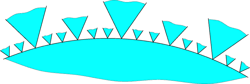
Figure 6. An infinite set of stability zones $\Omega_{\beta}$ adjacent to the boundary of a zone $\Omega_{\alpha}$

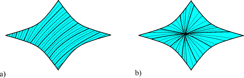
Figure 7. Everywhere dense families of directions $\mathbf{B}$ in stability zones for which the system (2.1) has periodic open trajectories, in the cases where the zone does not contain (a) and contains (b) the vector $\mathbf{l}_{\alpha}$

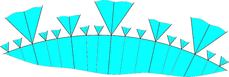
Figure 8. Curves of partially irrational directions $\mathbf{B}$ corresponding to the presence of periodic trajectories of (2.1) in adjacent stability zones

We are not aware of any other general results on the geometry of an individual stability zone. It can be seen from Fig. 5 that the stability zones are not necessarily convex. Moreover, the stability zones can be non-simply connected. The corresponding example can be constructed as follows.

Example 2.7.

Let the level surface of the dispersion law have the shape shown in Fig. 9. Namely, the surface consists of a family of parallel planes connected by thin curved tubes, each tube being contained in a small neighborhood of a plane parallel to a fixed plane $\Pi_{0}$ and being symmetric with respect to it. Then each family of parallel planes forming a not too small angle with $\Pi_{0}$ cuts all these tubes along closed curves. One can see from the constructions of the works [11, 13] that in this case all non-closed components of sections of this surface by planes from this family will be topologically regular.

Thus, in this case, all directions $\mathbf{B}$ that are not too close to the normal to the $\Pi_{0}$ plane will be in the same stability zone. At the same time, it can be shown that this stability zone will not cover the entire sphere.

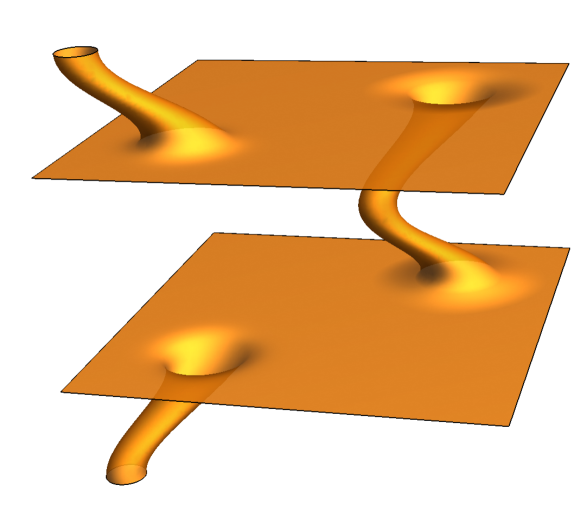
Figure 9. Fundamental domain of the surface for which a non-simply connected stability zone arises

The functions $\epsilon_{1}$ and $\epsilon_{2}$ introduced in Lemma 2.3, generally speaking, need not be continuous on the entire sphere. However, as noted in [14], they become continuous when restricted to the set of completely irrational directions $\mathbf{B}$, coinciding on this set with the restriction of some functions $\widetilde{\epsilon}_{1}(\mathbf{B})$, $\widetilde{\epsilon}_{2}(\mathbf{B})$ well defined and continuous on the entire unit sphere $\mathbb{S}^{2}$. Inside the stability zones, these functions are also uniquely characterized by the fact that $(\widetilde{\epsilon}_{1}(\mathbf{B}),\widetilde{\epsilon}_{2}(\mathbf{B}))$ is the largest range of energies $\epsilon_{0}$ for which system (2.1) has stable topologically regular trajectories.

For rational and partially irrational directions $\mathbf{B}$, the values of $\epsilon_{s}(\mathbf{B})$ and $\widetilde{\epsilon}_{s}(\mathbf{B})$ may not coincide due to the presence of unstable topologically regular trajectories at energy levels outside the interval $(\widetilde{\epsilon}_{1}(\mathbf{B}),\widetilde{\epsilon}_{2}(\mathbf{B}))$. In this case, we always have the inequalities

$$\epsilon_{1}(\mathbf{B})\leqslant\widetilde{\epsilon}_{1}(\mathbf{B})\leqslant\widetilde{\epsilon}_{2}(\mathbf{B})\leqslant\epsilon_{2}(\mathbf{B}).$$

Interior points of the stability zones $\Omega_{\alpha}$ are defined by the relation $\widetilde{\epsilon}_{1}(\mathbf{B})<\widetilde{\epsilon}_{2}(\mathbf{B})$. The relation $\widetilde{\epsilon}_{1}(\mathbf{B})=\widetilde{\epsilon}_{2}(\mathbf{B})$ takes place at the boundaries of the stability zones, as well as at the accumulation points of an infinite number of zones $\Omega_{\alpha}$ decreasing in size.

Here we would like to describe the structure of complex angle diagrams in some more detail and point out a number of important additional features of such diagrams. Let’s start by considering the rational directions of the magnetic field, which, in a sense, take a special place in an angular diagram.

As we have already said, rational directions $\mathbf{B}$ differ from other directions, in particular, in that the patterns of trajectories in different planes orthogonal to $\mathbf{B}$ can differ significantly from each other when $\mathbf{B}$ is rational. All non-singular open trajectories of the system (2.1), as well as open trajectories in our generalized sense, are periodic in all such planes.

For rational directions $\mathbf{B}$, it is typical that at some energy levels in the interval $[\epsilon_{1}(\mathbf{B}),\epsilon_{2}(\mathbf{B})]$ periodic complexes of stationary points and separatrices are present (Fig. 2). To each such complex we assign its rank which is the dimension of the sublattice in $H_{1}(\mathbb{T}^{3};\mathbb{Z})$ generated by all the separatrix cycles contained in the image of this complex under the projection onto the torus $\mathbb{T}^{3}=\mathbb{R}^{3}/\mathbb{Z}^{3}$. For example, for the complexes in Fig. 2 a)–c) this rank is equal to one, and for the complex in Fig. 2 d) it is two. For a fixed rational direction $\mathbf{B}$, the presence of such complexes of ranks zero and one is typical, while the presence of complexes of rank two requires some additional conditions (certain symmetry or conditions of codimension 1). As follows from the results of [11, 13, 14], if for a given rational direction $\mathbf{B}$ at least for one energy value

$$\epsilon\in[\epsilon_{1}(\mathbf{B}),\epsilon_{2}(\mathbf{B})]$$

there are only regular trajectories and/or complexes of stationary points and separatrices of rank $\leqslant 1$ in all planes orthogonal to $\mathbf{B}$, then the given direction $\mathbf{B}$ lies inside some stability zone $\Omega_{\alpha}$. It is natural to call rational directions $\mathbf{B}$ of this type ordinary rational directions.

Rational directions $\mathbf{B}$ such that, for any value of $\epsilon\in[\epsilon_{1}(\mathbf{B}),\epsilon_{2}(\mathbf{B})]$, there is a complex of stationary points and separatrices of rank two in at least one plane orthogonal to $\mathbf{B}$, we will call special rational directions.

Special rational directions $\mathbf{B}$ can appear in different parts of an angle diagram. For example, suppose that, for some rational direction $\mathbf{B}$, there is a periodic complex of separatrices shown in Fig. 2,d in one of the planes $\Pi$ orthogonal to $\mathbf{B}$. The shown complex contains, up to a shift by a reciprocal lattice vector, two saddle points in the $\mathbf{p}$-space connected by separatrices.

Let us first assume that the gradients of the function $\epsilon(\mathbf{p})$ at these points are codirectional. Then, for small shifts of the plane keeping its direction, the shown complex splits into closed non-singular trajectories of system (2.1). In this case, however, the type of such trajectories (electron or hole) is different for shifts in opposite directions.

It can be shown that the direction $\mathbf{B}$ lies in this case inside some stability zone $\Omega_{\alpha}$, and the corresponding plane $\Gamma_{\alpha}$ is parallel to $\Pi$.

The described situation provides an example when a stability zone $\Omega_{\alpha}$ contains the direction orthogonal to the corresponding plane $\Gamma_{\alpha}$. In this case, the planes orthogonal to $\mathbf{B}$ may contain periodic trajectories of different directions, periodic trajectories of a single direction, or not contain regular periodic trajectories at all. The different cases that arise in this situation, in particular, give different regimes of behavior of the conductivity tensor in strong magnetic fields (see [16], for example).

Let us now consider the situation when the gradients $\epsilon(\mathbf{p})$ at nonequivalent saddle points in Fig. 2, d are opposite to one another. Then, for small shifts of the plane $\Pi$ keeping its direction, the shown complex splits into periodic regular trajectories of system (2.1), which are stable under small changes of the energy $\epsilon$, as well as under small rotations of the direction of $\mathbf{B}$ around their mean direction. For close partially irrational directions $\mathbf{B}$ obtained as a result of such rotations, the non-degeneracy of the interval $[\epsilon_{1}(\mathbf{B}),\epsilon_{2}(\mathbf{B})]$ means that such a direction belongs to some stability zone $\Omega_{\alpha}$ or its boundary. It can be seen, therefore, that if the original direction $\mathbf{B}$ does not belong to any stability zone or its boundary, it always represents an accumulation point of of stability zones on the angular diagram.

The above argument is, in fact, of a general nature, which allows us to conclude that any special rational direction $\mathbf{B}$ either belongs to some stability zone (or its boundary), or is an accumulation point of stability zones $\Omega_{\alpha}$ on an angle diagram. In particular, the above arguments imply the assertion of the theorem 2.4 that the union of all stability zones $\Omega_{\alpha}$ is everywhere dense on the unit sphere $\mathbb{S}^{2}$.

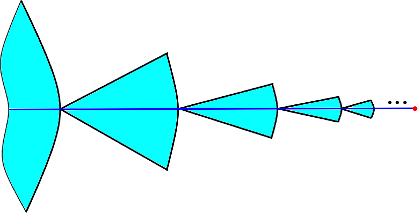
Figure 10. A sequence of stability zones, united by one direction of periodic open trajectories, converging to some special rational direction $\mathbf{B}$ (schematically)

In addition to special rational directions $\mathbf{B}$, the directions $\mathbf{B}$ for which the open trajectories of system (2.1) are chaotic are also accumulation points of stability zones. As we noted above, for such a direction of the magnetic field $\mathbf{B}$ chaotic trajectories present only at one energy level $\epsilon_{0}(\mathbf{B})$.

As we also said, the chaotic trajectories of system (2.1) can be divided into two main types: Tsarev-type trajectories and Dynnikov-type trajectories. The former can arise only for partially irrational directions $\mathbf{B}$ and always have an asymptotic direction in the $\mathbf{p}$-space ([10, 13]). Unlike regular open trajectories, Tsarev-type chaotic trajectories are generally not limited to straight strips of finite width in planes orthogonal to $\mathbf{B}$ (Fig. 11). The contribution of Tsarev-type trajectories to the magnetic conductivity is generally similar to the contribution of topologically regular trajectories, although it also has some special features.

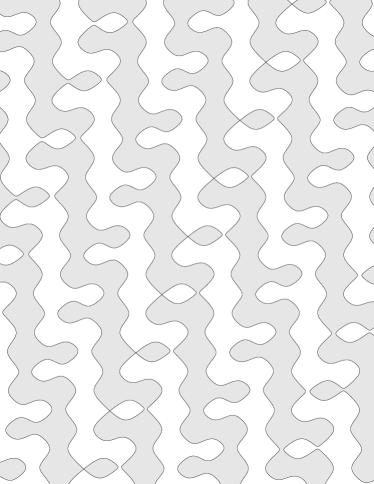
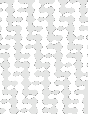
Figure 11. Examples of topologically regular trajectories and trajectories of Tsarev’s type in a plane orthogonal to $\mathbf{B}$

A necessary condition for the presenece of Tsarev-type trajectories is the presence on the corresponding level surface

$$\epsilon(\mathbf{p})=\epsilon_{0}$$

of separatrix cycles that are nonhomologous to zero in the torus $\mathbb{T}^{3}$. As a consequence of this, the corresponding direction $\mathbf{B}$ must be orthogonal to some rational direction in the $\mathbf{p}$-space, but itself should not be rational. Thus, directions $\mathbf{B}$ for which Tsarev-type chaotic trajectories occur are naturally combined into families, each of which is contained in a great circular arc lying in some integral plane of the crystal lattice, and consists of all partially irrational points of this arcs. The rational points of these arcs can then be boundary points of stability zones, as well as accumulation points of stability zones (special rational directions $\mathbf{B}$), see Fig. 12.

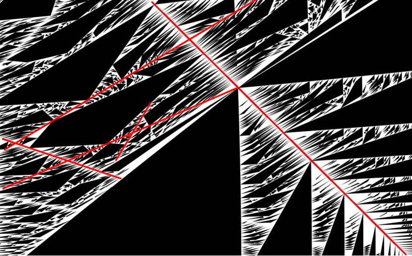
Figure 12. Stability zones and lines of appearance of Tsarev’s trajectories for a surface $\cos p_{x}+\cos p_{y}+\cos p_{z}=0$

A more complex type of chaotic trajectories of system (2.1) are Dynnikov-type trajectories ([13]). Trajectories of this type correspond to pronounced chaotic dynamics both in planes orthogonal to $\mathbf{B}$ (Fig. 13) and on the Fermi surface considered as a compact surface in $\mathbb{T}^{3}$. A consequence of such dynamics is the emerging of nontrivial regimes of the behavior of conductivity in the presence of such trajectories on the Fermi surface ([17, 18]), among which especially noticeable is the suppression of the conductivity in the direction of the magnetic field, as well as the presence of fractional powers of $B$ in the asymptotics of the conductivity tensor. According to S.P. Novikov’s conjecture [49], the set of directions $\mathbf{B}$ corresponding to chaotic regimes (of any type) for a fixed generic dispersion relation has measure zero and the Hausdorff dimension strictly less than 2 on the angular diagram. This conjecture is partially confirmed in the following statement proved in a paper under preparation by I.Dynnikov, P.Hubert, P.Mercat, O.Paris-Romaskevich, and A.Skripchenko.

Theorem 2.8.

For a generic dispersion relation $\epsilon$ obeying central symmetry, $\epsilon(\mathbf{p})=\epsilon(-\mathbf{p})$, and such that all its level surfaces viewed in $\mathbb{T}^{3}$, have genus at most three, the set of directions $\mathbf{B}$ yielding chaotic regimes has measure zero.

Figure 13. Chaotic Dynnikov-type trajectory lying on the surface $\cos p_{x}+\cos p_{y}+\cos p_{z}=0$

The study of chaotic trajectories of Dynnikov’s type is actively keep going at the present time; below we describe some of the most recent results obtained in this area.

Theorem 2.9 ([29]).

Let the surface $\epsilon(\mathbf{p})=\epsilon_{0}$ and the magnetic field $\mathbf{B}$ be such that the trajectories of system (2.1) are chaotic, and the direction $\mathbf{B}$ is completely irrational. Then in almost all planes orthogonal to $\mathbf{B}$ the number of open trajectories is the same and equals either one, or two, or is infinite.

The least difficult is to construct examples for which there is exactly one chaotic trajectory in almost every plane orthogonal to $\mathbf{B}$. For example, all “self-similar” examples (see [32]) in the case of a surface of genus three have this property.

In the papers [33, 34], examples of chaotic regimes in Novikov’s problem are constructed, for which each plane orthogonal to $\mathbf{B}$ contains an infinite number of open trajectories, and these trajectories have an asymptotic direction, but are not contained in straight strips of finite width. This effect is related to the absence of unique ergodicity of the corresponding foliation on a compact level surface $\epsilon=\epsilon_{0}$ in $\mathbb{T}^{3}$, and requires a very subtle choice of system parameters. Apparently, among the chaotic regimes in Novikov’s problem, such a situation is not typical.

No examples are currently known in which almost every plane orthogonal to $\mathbf{B}$ contains exactly two chaotic trajectories. We only know that they do not exist in the case of genus three [29].

When considering galvanomagnetic phenomena in metals, we must take into account only the trajectories of system (2.1) that lie at the Fermi level. Accordingly, it is natural to introduce angular diagrams showing the presence of open trajectories, as well as their type, on the Fermi surface $\epsilon(\mathbf{p})=\epsilon_{\mathrm{F}}$ for different directions of the magnetic field. Such diagrams, of course, are poorer than the diagrams for the total dispersion relation, and contain domains consisting of directions $\mathbf{B}$ for which all trajectories at the Fermi level are closed (see e.g. Fig. 14). The stability zones on such diagrams are defined as closures of the connected components of the set of directions $\mathbf{B}$ for which system (2.1) has stable topologically regular open trajectories at the level $\epsilon=\epsilon_{F}$ .

Each stability zone $\Omega^{*}_{\alpha}$ on such diagrams, as before, is a domain with a piecewise smooth boundary on the unit sphere. It is characterized by some values of the topological invariants $(m^{1}_{\alpha},m^{2}_{\alpha},m^{3}_{\alpha})$ and is a subdomain of the corresponding zone $\Omega_{\alpha}$ defined for the entire dispersion relation.

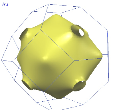
Figure 14. The Fermi surface of gold and the corresponding exact mathematical stability zones in the angular diagram ([56, 57])

If, however, we are talking about the complete family of open trajectories on the Fermi surface associated with a given stability zone $\Omega_{\alpha}$, then the corresponding set of directions $\mathbf{B}$ goes beyond the zone $\Omega^{*}_{\alpha}$. The reason for this is the presence of unstable periodic trajectories for some partially irrational directions $\mathbf{B}$ located near the boundaries of each of the zones $\Omega^{*}_{\alpha}$. Such directions form extensions of arcs of partially irrational directions $\mathbf{B}$, corresponding to the presence of stable periodic trajectories in the zone $\Omega^{*}_{\alpha}$, beyond the boundaries of this zone (Fig. 15). Adjacent segments form an everywhere dense set at the boundary of a stability zone, and their length tends to zero as the period of the corresponding trajectories increases.

As was shown in [58], such a structure leads to rather complex analytic properties of the magnetic conductivity tensor both inside the zones $\Omega^{*}_{\alpha}$ and near their boundaries. As observed in [59], for experimental determination of the exact boundaries of the zones $\Omega^{*}_{\alpha}$, it may be better to use methods other than direct measurements of conductivity in strong magnetic fields.

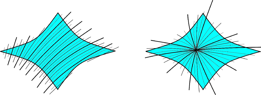
Figure 15. Complete sets of directions $\mathbf{B}$ inside one stability zone $\Omega_{\alpha}$ corresponding to the presence of open trajectories on the Fermi surface

Certainly, angular diagrams for specific Fermi surfaces can be very simple. For example, they can entirely consist of directions $\mathbf{B}$ for which all trajectories of system (2.1) are closed, or they can admit only unstable periodic trajectories for some $\mathbf{B}$ (Fig. 16).

Certain restrictions on the structure of an angular diagram are imposed by the topology of the Fermi surface and its embeddings in the torus $\mathbb{T}^{3}$. An important role here is played by such characteristic as the dimension of the image of its one-dimensional homology in the one-dimensional homology of the torus $\mathbb{T}^{3}$

$$H_{1}\left(S_{\mathrm{F}}\right)\rightarrow H_{1}\left(\mathbb{T}^{3}\right),$$

which we call the topological rank of the Fermi surface. It obviously can take the values 0, 1, 2, and 3. Angular diagrams containing stability zones can only emerge for Fermi surfaces of topological rank two or more, and more than one stability zone can exist only if the topological rank is three. Note that Fermi surfaces of rank 3 must have genus $g\geqslant 3$.

Figure 16. Fermi surfaces corresponding to the simplest angle diagrams

As for the presence of directions $\mathbf{B}$ on the angular diagrams for Fermi surfaces that are not included in any of the stability zones, but which are the limit points of the union of all stability zones, then such a situation is possible only when the diagram of the entire dispersion relation contains an infinite number of stability zones. Such directions $\mathbf{B}$ will be called singular for a given Fermi surface. As noted in [60], the presence of singular directions requires that the Fermi energy $\epsilon_{\mathrm{F}}$ falls into a rather narrow energy interval, determined by the dispersion relation $\epsilon(\mathbf{p})$.

Namely, consider some fixed periodic function (dispersion relation) $\epsilon(\mathbf{p})$, taking values in a certain interval

$$\epsilon_{\rm min}\leqslant\epsilon(\mathbf{p})\leqslant\epsilon_{\rm max}.$$

It is easy to see that for values of $\epsilon_{\mathrm{F}}$ close to $\epsilon_{\rm min}$ or $\epsilon_{\rm max}$, the Fermi surfaces is very simple, and the angular diagrams corresponding to them are trivial (all trajectories of the system (2.1) are closed). One can introduce values $\epsilon^{\mathcal{A}}_{1}$, $\epsilon^{\mathcal{A}}_{2}$,

$$\epsilon_{\rm min}<\epsilon^{\mathcal{A}}_{1}<\epsilon^{\mathcal{A}}_{2}<\epsilon_{\rm max},$$

such that for the values of the Fermi energy $\epsilon_{\mathrm{F}}$ lying in the interval $(\epsilon^{\mathcal{A}}_{1},\epsilon^{\mathcal{A}}_{2})$, the corresponding angular diagrams will contain stability zones.

The resulting angle diagrams, in turn, can also be divided into two classes (diagrams of type A and diagrams of type B), which differ qualitatively. Namely:

1) generic diagrams of type A contain only a finite number of stability zones, while everywhere in the domain corresponding to the presence of only closed trajectories on the Fermi surface, the respective Hall (transverse) conductivity has the same type (electron or hole) (Fig.   17(a));

2) generic diagrams of type B contain an infinite number of stability zones, and in the domain corresponding to the presence of only closed trajectories on the Fermi surface, there are both domains corresponding to electronic Hall conductivity and domains corresponding to hole Hall conductivity (Fig. 17(b)).

Figure 17. Complex angle diagrams of type A (a) and type B (b) (schematically). The letters e and h denote the type of the Hall conductivity in the domains corresponding to the presence of only closed trajectories on the Fermi surface (electron and hole, respectively)

For generic dispersion relations we can define a finite energy interval $(\epsilon^{\mathcal{B}}_{1},\epsilon^{\mathcal{B}}_{2})$,

$$\epsilon^{\mathcal{A}}_{1}<\epsilon^{\mathcal{B}}_{1}<\epsilon^{\mathcal{B}}_{2}<\epsilon^{\mathcal{A}}_{2},$$

such that for all values of $\epsilon_{\mathrm{F}}$ from this interval the corresponding angular diagrams are of type B, while the values of $\epsilon_{\mathrm{F}}$ from the intervals $(\epsilon^{\mathcal{A}}_{1},\epsilon^{\mathcal{B}}_{1})$ and $(\epsilon^{\mathcal{B}}_{2},\epsilon^{\mathcal{A}}_{2})$ correspond to angle diagrams of type A.

Generic diagrams of type A do not contain singular directions ${\bf B}$. On the contrary, generic diagrams of type B must contain them. We also note here that, since the Fermi levels at which special rational directions $\mathbf{B}$ can arise have measure zero, for generic values $\epsilon_{\mathrm{F}}$ from the interval $(\epsilon^{\mathcal{B}}_{1},\epsilon^{\mathcal{B}}_{2})$ singular directions $\mathbf{B}$ will correspond to the presence of chaotic trajectories of Tsarev’s or Dynnikov’s type.

It is shown in [14] that the measure of the set of directions $\mathbf{B}$ corresponding to the presence of chaotic trajectories on a generic Fermi surface is equal to zero. According to S.P. Novikov’s conjecture ([50, 51]), the Hausdorff dimension of this set for generic surfaces is strictly less than 1.

In conclusion, we note here that, apparently, the length of the interval $(\epsilon^{\mathcal{B}}_{1},\epsilon^{\mathcal{B}}_{2})$ for actual dispersion relations is rather small, which, perhaps, explains the absence, to date, of clear evidence of chaotic trajectories of system (2.1) in experiments with real conductors. It is also possible, of course, that unfamiliarity with trajectories of this type until very recently did not allow to interpret certain experimental data appropriately. However, we hope that trajectories of this type, as well as the respective behavior of the magnetic conductivity, will anyway be discovered in the future for suitable classes of conductors among the huge variety of new materials currently being produced.

3. General Novikov’s problem. Setting and results.

As we said in the Introduction, the general Novikov’s problem is to describe the geometry of open level lines of a quasi-periodic function having an arbitrary number of quasi-periods on the plane. One of the most natural formulations is to describe the level lines of a family of functions obtained by compose a given generic $N$-periodic function $F$ on the space $\mathbb{R}^{N}$ with all possible affine embeddings $\iota:\mathbb{R}^{2}\rightarrow\mathbb{R}^{N}$. The global properties of level lines of our interest depend primarily on the direction of the plane $\iota(\mathbb{R}^{2})$, which is a point of the Grassmann manifold $G_{N,2}$, and may also depend on the shift parameters. The change of affine coordinates in $\mathbb{R}^{2}$ does not play any role for us.

The most essential result in Novikov’s problem for $N>3$ is the following statement.

Theorem 3.1 ([47, 48]).

There is an open everywhere dense subset $S\subset C^{\infty}(\mathbb{T}^{4})$ of 4-periodic functions $F$, and an open everywhere dense subset $X_{F}\subset G_{4,2}$ depending on $F$ such that for any $\xi\in X_{F}$, any level line of the restriction of the function $F$ onto any two-dimensional plane of direction $\xi$ in $\mathbb{R}^{4}$ is contained in a straight strip of finite width. The widths of these strips, as well as the diameters of the compact level lines, are bounded above by a constant that depends only on the pair $(F,\xi)$, and any open non-singular level line passes through the corresponding strip (Fig. 4). The directions of the strips containing open level lines are orthogonal to some integer vector $(m^{1},m^{2},m^{3},m^{4})$ which is a locally constant function of $(F,\xi)$.

It is easy to see that the situation of stable “topologically regular” behavior of the level lines of a quasi-periodic function on the plane can occur for any number of quasi-periods. For example, it will take place if for the corresponding $N$-periodic function in $\mathbb{R}^{N}$ we take a small perturbation of a periodic function depending on only one coordinate. Thus, for a family of quasi-periodic functions obtained as restrictions of a fixed $N$-periodic function to all possible planes, one can also define stability zones, which are open domains in $G_{N,2}$. It should be noted, however, that with an increase in the number of quasiperiods, the shape of topologically regular level lines often is getting more complicated, approaching chaotic behavior on finite scales. In general, as the number of quasi-periods increases, Novikov’s problem approaches more and more a problem on random potentials in the two-dimensional plane.

Below we present a number of topological results related to Novikov’s problem with an arbitrary number of quasi-periods that generalize the previously known statements for the case $N=3$.

Lemma 3.2.

Let $F(z^{1},\dots,z^{N})$ be an $N$-periodic function with respect to some integer lattice in $\mathbb{R}^{N}$, and let  $\xi\in G_{N,2}$ and $c\in\mathbb{R}$ be such that for any two-dimensional affine plane $\Pi$ of direction $\xi$ all level lines $F|_{\Pi}=c$ are compact. Then the diameters of all these level lines are bounded from above by one constant common to all planes of direction $\xi$.

This fact follows from the compactness of the image of the surface $F=c$ in the torus $\mathbb{T}^{N}$: each compact level line (both singular and non-singular) has a neighborhood of finite diameter such that all other level lines $F=c$ in parallel planes that intersect this neighborhood lie entirely in it. From such neighborhoods, one can choose a finite family so that their images cover the entire image of the surface $F=c$ in the torus $\mathbb{T}^{N}$.

Note that in the case $N=3$ the assumption that all level lines $F=c$ are compact in all planes of a given direction is not required (see Lemma 2.1).

Theorem 3.3.

Let $F(z^{1},\dots,z^{N})$ be an $N$-periodic function, and let $\xi\in G_{N,2}$ be a fixed direction of two-dimensional planes in $\mathbb{R}^{N}$. Then the set of values $c\in\mathbb{R}$ such that for some plane $\Pi$ of direction $\xi$ the level set $F|_{\Pi}=c$ has unbounded components forms a closed interval $[c_{1},c_{2}]$ or consists of a single point $c_{0}$.

The proof mostly follows the lines of the proof of a similar assertion for the case $N=3$ given in [13, 14]. Note that there is again a difference from the case $N=3$, which consists in the fact that we consider the entire set of planes of one direction simultaneously, while in the case of three quasi-periods the statement was true for each individual plane of this direction. In the case of more than three quasi-periods, we admit a situation in which all level lines $F|_{\Pi}=c\in[c_{1},c_{2}]$ in some planes $\Pi$ of direction $\xi$ are compact, but their diameters are not limited from above.

Note, that if $\xi$ is a completely irrational direction, which is not contained in a hyperplane of rational direction, then for any $c\in[c_{1},c_{2}]$ (or $c=c_{0}$) and any plane $\Pi$ of direction $\xi$, the level set $F|_{\Pi}=c$ has either unbounded or arbitrarily large closed components.

Indeed, let there be a plane $\Pi$ of direction $\xi$, in which there are only closed level lines $F|_{\Pi}=c$, the size of which is limited by one constant. By the size of a trajectory we mean the minimum diameter of the circle $D$ in which it can be placed.

Let’s take a plane of direction $\xi$, in which there is an unbounded level line. Let us take a segment of this level line such that it does not contain singular points and cannot be enclosed in a circle of diameter $D$. There is a small $\delta$ such that this segment is preserved for all parallel shifts of this plane in all transversal directions by a distance less than $\delta$.

Consider the corresponding $\delta$ neighborhood $O$ of our plane (which contains unbounded components). Integer shifts of the original plane $\Pi$ are everywhere dense in $R^{N}$ for our embedding and must fall in a neighborhood $O$. We get a contradiction.

Recall once again that we call here unbounded components not only non-singular level lines, but also connected complexes containing singular points and separatrices connecting them, unbounded in the plane (the same for bounded components). We also impose general position conditions for completely irrational embeddings, namely, we require that each such complex contains at most a finite number of multiple saddles (of finite multiplicity).

We would also like to note here that the statements formulated above can also be generalized to a more general case, namely, the case of level surfaces of generic quasi-periodic functions in $\mathbb{R}^{n}$ with $N$ quasi-periods. The proofs of the corresponding assertions here are similar to those given above under the imposition of natural conditions of general position.

As can also be shown, the situation can be described more precisely in the important nongeneric case of the Novikov problem.

Theorem 3.4.

Let $F(z^{1},\dots,z^{N})$ be an $N$-periodic function, and let $\xi\in G_{N,2}$ be a fixed direction of two-dimensional planes containing exactly one, up to a factor, non-zero integer vector and not contained in a rational hyperplane. Then the following is true for all planes $\Pi$ of direction $\xi$:

1. all non-singular open level lines of the function $F|_{\Pi}$ have an asymptotic direction, which is the same, up to sign, for all planes of the direction $\xi$;

2. for a fixed $c$, the diameters of all compact level lines $F|_{\Pi}=c$ are bounded from above by a single constant common to all planes of the direction $\xi$;

3. if, for some $c$, there are non-periodic unbounded level lines $F|_{\Pi}=c$ in some plane $\Pi$, then they also exist in any other plane of direction $\xi$.

The proof of the first part follows the proof of a similar assertion for $N=3$ given in [13, §6]. Now, we take for $\gamma$ a path in $\mathbb{R}^{N}$ that lies entirely in some plane of direction $\xi$ and such that the end point of the path $\gamma$ is obtained from the initial point by a shift by $\mathbf{w}$, where $\mathbf{w}$ is an irreducible nonzero integer vector parallel to $\xi$. Among all such paths, we choose the one that has the least number of intersection points with the surface $F=c$. Next, in the orthogonal complement $\xi^{\perp}$, we choose a small neighborhood $W$ of the origin so that the shift of $\gamma$ by vectors from $W$ does not increase the number of intersection points with the surface $F=c$ . The union $\Gamma$ of all shifts of $\gamma$ by all possible vectors of the form $\mathbf{u}+\mathbf{v}$, where $\mathbf{u}\in W$, $\mathbf{v}\in\mathbb{Z}^{N}$, will cut each plane of direction $\xi$ into strips of a finite number of shapes, following in a “quasi-periodic” order, and in each strip the pattern of level lines is periodic. The rest of the argument does not differ from the case $N=3$.

The second and third assertions of the theorem are proved using the same construction. Compact level lines $F=c$ in the planes of direction $\xi$ do not intersect $\Gamma$, which means that they are contained in strips of limited width in which the pattern of intersection lines is invariant under the shift by the vector $\mathbf{w}$. This entails the existence of a general upper bound for the diameters of these level lines.

The presence of non-periodic unbounded level lines $F=c$ in any of the planes of direction $\xi$ is equivalent to the fact that the intersection of the surface $F=c$ with $\Gamma$ is non-empty. This implies the third assertion of the theorem.

Note that, as in the case of $N=3$, the presence of an asymptotic direction of the level lines in the last theorem does not mean that these level lines lie in straight strips of finite width.

References

- [1] H. Bohr., Zur theorie der fastperiodischen funktionen., Acta Mathematica, 47(3) (1926), 237-281
- [2] A.S. Besicovitch., On generalized almost periodic functions., Proceedings of the London Mathematical Society, 2(1) (1926), 495-512
- [3] S.P. Novikov., The Hamiltonian formalism and a many-valued analogue of Morse theory., Russian Math. Surveys 37 (5), 1-56 (1982).
- [4] I.M. Lifshitz, M.Ya. Azbel, M.I. Kaganov., The Theory of Galvanomagnetic Effects in Metals., Sov. Phys. JETP 4:1, 41-53 (1957).
- [5] I.M. Lifshitz, V.G. Peschansky., Galvanomagnetic characteristics of metals with open Fermi surfaces., Sov. Phys. JETP 8:5, 875-883 (1959).
- [6] I.M. Lifshitz, V.G. Peschansky., Galvanomagnetic characteristics of metals with open Fermi surfaces. II., Sov. Phys. JETP 11:1, 131-141 (1960).
- [7] I.M. Lifshitz, M.Ya. Azbel, M.I. Kaganov., Electron Theory of Metals. New York: Consultants Bureau, 1973.
- [8] A.V. Zorich., A problem of Novikov on the semiclassical motion of an electron in a uniform almost rational magnetic field., Russian Math. Surveys 39 (5), 287-288 (1984).
- [9] I.A. Dynnikov., Proof of S.P. Novikov’s conjecture for the case of small perturbations of rational magnetic fields., Russian Math. Surveys 47:3, 172-173 (1992).
- [10] S.P. Tsarev, private communication, 1992-1993
- [11] I.A. Dynnikov., Proof of S.P. Novikov’s conjecture on the semiclassical motion of an electron., Math. Notes 53:5, 495-501 (1993).
- [12] I.A. Dynnikov., Surfaces in 3-torus: geometry of plane sections., Proc. of ECM2, BuDA, 1996.
- [13] I.A. Dynnikov., Semiclassical motion of the electron. A proof of the Novikov conjecture in general position and counterexamples., Solitons, geometry, and topology: on the crossroad, Amer. Math. Soc. Transl. Ser. 2, 179, Amer. Math. Soc., Providence, RI, 1997, 45-73.
- [14] I.A. Dynnikov., The geometry of stability zones in Novikov’s problem on the semiclassical motion of an electron., Russian Math. Surveys 54:1, 21-59 (1999).
- [15] S.P. Novikov, A.Y. Maltsev., Topological quantum characteristics observed in the investigation of the conductivity in normal metals., JETP Letters 63 (10), 855-860 (1996).
- [16] S.P. Novikov, A.Y. Maltsev., Topological phenomena in normal metals., Physics-Uspekhi 41:3, 231-239 (1998).
- [17] A.Ya. Maltsev., Anomalous behavior of the electrical conductivity tensor in strong magnetic fields., Journal of Experimental and Theoretical Physics 85 (5), 934-942 (1997)
- [18] A.Ya. Maltsev, S.P. Novikov., The Theory of Closed 1-Forms, Levels of Quasiperiodic Functions and Transport Phenomena in Electron Systems., Proceedings of the Steklov Institute of Mathematics 302, 279-297 (2018).
- [19] A.V. Zorich., Asymptotic Flag of an Orientable Measured Foliation on a Surface., Proc. Geometric Study of Foliations, (Tokyo, November 1993), ed. T.Mizutani et al. Singapore: World Scientific Pb. Co., 479-498 (1994).
- [20] A.V. Zorich., Finite Gauss measure on the space of interval exchange transformations. Lyapunov exponents., Annales de l’Institut Fourier 46:2, (1996), 325-370.
- [21] Anton Zorich., On hyperplane sections of periodic surfaces., Solitons, Geometry, and Topology: On the Crossroad, V. M. Buchstaber and S. P. Novikov (eds.), Translations of the AMS, Ser. 2, vol. 179, AMS, Providence, RI (1997), 173-189.
- [22] Anton Zorich., Deviation for interval exchange transformations., Ergodic Theory and Dynamical Systems 17, (1997), 1477-1499.
- [23] Anton Zorich., How do the leaves of closed 1-form wind around a surface., Pseudoperiodic Topology, V.I.Arnold, M.Kontsevich, A.Zorich (eds.), Translations of the AMS, Ser. 2, vol. 197, AMS, Providence, RI, 1999, 135-178.
- [24] R. De Leo., Existence and measure of ergodic leaves in Novikov’s problem on the semiclassical motion of an electron., Russian Math. Surveys 55:1 (2000), 166-168.
- [25] R. De Leo., Characterization of the set of “ergodic directions” in Novikov’s problem of quasi-electron orbits in normal metals., Russian Math. Surveys 58:5 (2003), 1042-1043.
- [26] R. De Leo., Topology of plane sections of periodic polyhedra with an application to the Truncated Octahedron., Experimental Mathematics 15:1 (2006), 109-124.
- [27] Anton Zorich., Flat surfaces., in collect. ¡¡Frontiers in Number Theory, Physics and Geometry. Vol. 1: On random matrices, zeta functions and dynamical systems; Ecole de physique des Houches, France, March 9-21 2003, P. Cartier; B. Julia; P. Moussa; P. Vanhove (Editors), Springer-Verlag, Berlin, 2006, 439-586.
- [28] R. De Leo, I.A. Dynnikov., An example of a fractal set of plane directions having chaotic intersections with a fixed 3-periodic surface., Russian Math. Surveys 62:5 (2007), 990-992.
- [29] I.A. Dynnikov., Interval identification systems and plane sections of 3-periodic surfaces., Proceedings of the Steklov Institute of Mathematics 263:1 (2008), 65-77.
- [30] R. De Leo, I.A. Dynnikov., Geometry of plane sections of the infinite regular skew polyhedron ., Geom. Dedicata 138:1 (2009), 51-67.
- [31] A. Skripchenko., Symmetric interval identification systems of order three., Discrete Contin. Dyn. Sys. 32:2 (2012), 643-656.
- [32] A. Skripchenko., On connectedness of chaotic sections of some 3-periodic surfaces., Ann. Glob. Anal. Geom. 43 (2013), 253-271.
- [33] I. Dynnikov, A. Skripchenko., On typical leaves of a measured foliated 2-complex of thin type., Topology, Geometry, Integrable Systems, and Mathematical Physics: Novikov’s Seminar 2012-2014, Advances in the Mathematical Sciences., Amer. Math. Soc. Transl. Ser. 2, 234, eds. V.M. Buchstaber, B.A. Dubrovin, I.M. Krichever, Amer. Math. Soc., Providence, RI, 2014, 173-200, arXiv: 1309.4884
- [34] I. Dynnikov, A. Skripchenko., Symmetric band complexes of thin type and chaotic sections which are not actually chaotic., Trans. Moscow Math. Soc., Vol. 76, no. 2, 2015, 287-308.
- [35] A. Avila, P. Hubert, A. Skripchenko., Diffusion for chaotic plane sections of 3-periodic surfaces., Inventiones mathematicae, October 2016, Volume 206, Issue 1, pp 109-146.
- [36] A. Avila, P. Hubert, A. Skripchenko., On the Hausdorff dimension of the Rauzy gasket., Bulletin de la societe mathematique de France, 2016, 144 (3), pp. 539–568.
- [37] L. Guidoni, B. Depret, A. di Stefano, and P. Verkerk, Atomic diffusion in an optical quasicrystal with five-fold symmetry, Phys. Rev. A, Vol. 60, Number 6 (1999), R4233-R4236
- [38] A.Ya. Maltsev, Quasiperiodic functions theory and the superlattice potentials for a two-dimensional electron gas, Journal of Mathematical Physics 45:3 (2004), 1128-1149.
- [39] L. Sanchez-Palencia and L. Santos, Bose-Einstein condensates in optical quasicrystal lattices, Phys. Rev. A 72 (2005), 053607
- [40] Konrad Viebahn, Matteo Sbroscia, Edward Carter, Jr-Chiun Yu, and Ulrich Schneider, Matter-Wave Diffraction from a Quasicrystalline Optical Lattice, Phys. Rev. Lett. 122 (2019), 110404
- [41] Ronan Gautier, Hepeng Yao, and Laurent Sanchez-Palencia, Strongly Interacting Bosons in a Two-Dimensional Quasicrystal Lattice, Phys. Rev. Lett. 126 (2021), 110401
- [42] I.A. Dynnikov, A.Ya. Maltsev, Features of the motion of ultracold atoms in quasiperiodic potentials, JETP, 133 (6), 711-736 (2021)
- [43] D. Stauffer, Scaling theory of percolation clusters, Physics Reports, Volume 54, Issue 1 (1979), 1-74.
- [44] J.W. Essam, Percolation theory, Rep. Prog. Phys. 43 (1980), 833-912
- [45] Eberhard K. Riedel, The potts and cubic models in two dimensions: A renormalization-group description, Physica A: Statistical Mechanics and its Applications., Volume 106, Issues 1-2 (1981), 110-121.
- [46] S.A. Trugman, Localization, percolation, and the quantum Hall effect, Phys. Rev. B 27 (1983), 7539-7546
- [47] S.P. Novikov, Levels of quasiperiodic functions on a plane, and Hamiltonian systems, Russian Math. Surveys, 54 (5) (1999), 1031-1032
- [48] I.A. Dynnikov, S.P. Novikov, Topology of quasi-periodic functions on the plane, Russian Math. Surveys, 60 (1) (2005), 1-26
- [49] A.Ya. Maltsev, S.P. Novikov., Dynamical Systems, Topology and Conductivity in Normal Metals., arXiv:cond-mat/0304471
- [50] A.Ya. Maltsev, S.P. Novikov., Quasiperiodic functions and Dynamical Systems in Quantum Solid State Physics., Bulletin of Braz. Math. Society, New Series 34:1 (2003), 171-210.
- [51] A.Ya. Maltsev, S.P. Novikov., Dynamical Systems, Topology and Conductivity in Normal Metals in strong magnetic fields., Journal of Statistical Physics 115:(1-2) (2004), 31-46.
- [52] C. Kittel., Quantum Theory of Solids., Wiley, 1963.
- [53] J.M. Ziman., Principles of the Theory of Solids., Cambridge University Press 1972.
- [54] A.A. Abrikosov., Fundamentals of the Theory of Metals., Elsevier Science & Technology, Oxford, United Kingdom, 1988
- [55] Leo R.D. (2019) A Survey on Quasiperiodic Topology. In: Berezovskaya F., Toni B. (eds) Advanced Mathematical Methods in Biosciences and Applications. pp 53-88 STEAM-H: Science, Technology, Engineering, Agriculture, Mathematics & Health. Springer, Cham. DOI: https://doi.org/10.1007/978-3-030-15715-9_3
- [56] R. De Leo., Topological effects in the magnetoresistance of Au and Ag., Phys. Lett. A 332, 469-474 (2004)
- [57] R. De Leo., First-principles generation of stereographic maps for high-field magnetoresistance in normal metals: An application to Au and Ag., Physica B: Condensed Matter 362 (1-4) (2005), 62-75
- [58] A.Ya. Maltsev., On the Analytical Properties of the Magneto-Conductivity in the Case of Presence of Stable Open Electron Trajectories on a Complex Fermi Surface., Journal of Experimental and Theoretical Physics 124 (5), 805-831 (2017).
- [59] A.Ya. Maltsev, Oscillation phenomena and experimental determination of exact mathematical stability zones for magneto-conductivity in metals having complicated Fermi surfaces., Journal of Experimental and Theoretical Physics 125:5, 896-905 (2017).
- [60] A.Ya. Maltsev, The second boundaries of stability zones and the angular diagrams of conductivity for metals having complicated Fermi surfaces, Journal of Experimental and Theoretical Physics 127 (6), 1087-1111 (2018)