Eliminating Lipschitz Singularities in Diffusion Models

Abstract

Diffusion models, which employ stochastic differential equations to sample images through integrals, have emerged as a dominant class of generative models. However, the rationality of the diffusion process itself receives limited attention, leaving the question of whether the problem is well-posed and well-conditioned. In this paper, we uncover a vexing propensity of diffusion models: they frequently exhibit the infinite Lipschitz near the zero point of timesteps. This poses a threat to the stability and accuracy of the diffusion process, which relies on integral operations. We provide a comprehensive evaluation of the issue from both theoretical and empirical perspectives. To address this challenge, we propose a novel approach, dubbed E-TSDM, which eliminates the Lipschitz singularity of the diffusion model near zero. Remarkably, our technique yields a substantial improvement in performance, e.g., on the high-resolution FFHQ dataset ($256\times 256$). Moreover, as a byproduct of our method, we manage to achieve a dramatic reduction in the Frechet Inception Distance of other acceleration methods relying on network Lipschitz, including DDIM and DPM-Solver, by over 33%. We conduct extensive experiments on diverse datasets to validate our theory and method. Our work not only advances the understanding of the general diffusion process, but also provides insights for the design of diffusion models.

1 Introduction

The rapid development of diffusion models has been witnessed in image synthesis [10, 27, 23, 25, 24, 34, 11] in the past few years, whose success profits from modeling a complex data distribution with a cascade of simple distributions. Concretely, diffusion models construct a multi-step process to destroy a signal by gradually adding noises to it. That way, reversing the diffusion process (i.e., denoising) at each step naturally admits a sampling capability. In essence, the sampling process involves solving a reverse-time stochastic differential equation (SDE) through integrals [31].

Although diffusion models have achieved a great success in synthesizing images, the rationality of the diffusion process itself has received limited attention, leaving the open question of whether the problem is well-posed and well-conditioned. In this paper, we surprisingly observe that diffusion models often exhibit an alarming propensity to possess infinite Lipschitz near the zero point of timesteps. Such large Lipschitz constants represent a significant threat to the stability and accuracy of the diffusion process. We conduct a comprehensive investigation of this issue from both theoretical and empirical perspectives.

One of the most direct methods to reduce the Lipschitz constants is to impose restrictions on the Lipschitz constants using regularization techniques. However, this approach requires additional gradient calculations, which significantly reduces training efficiency and places higher demands on hardware resources. Another approach to controlling the Lipschitz constants is to modify the network architecture itself. However, it is challenging to limit the Lipschitz constants to some specific small values without introducing additional structures. Fortunately, there is a simple alternative solution: By sharing the timestep conditions in the interval with large Lipschitz constants, the Lipschitz constants can be set to zero.

Based on the analysis above, we propose a practical approach to address the issue of the large Lipschitz constants. Specifically, we divide the target interval with small noise levels into $n$ sub-intervals uniformly, and share the condition values between neighboring timesteps in each sub-interval, as illustrated in (II) of Fig. 1a. In this way, our approach can effectively reduce the Lipschitz constants near $t=0$ to zero. To validate this idea, we conduct extensive experiments, including unconditional generation on various datasets, acceleration of sampling using popular fast samplers, and a classical conditional generation task, i.e., super-resolution task. Both qualitative and quantitative results confirm that our approach substantially alleviates the large Lipschitz constants which occur in the intervals whose noise levels are small, and improves the synthesis performance compared to the DDPM baseline [10].

\begin{overpic}[width=433.62pt]{figures/first.pdf} \put(75.0,5.5){{$\tilde{t}$ (=100) }} \put(13.0,-1.0){(a) Conceptual comparison} \put(66.0,-1.0){(b) Lipschitz constants} \end{overpic}

Figure 1: (a) Conceptual comparison between DDPM [10] (I) and our proposed early timestep-shared diffusion model (E-TSDM) (II). DDPM [10] trains the network $\epsilon_{\theta}(\cdot,t)$ with varying timestep conditions $t$ at each denoising step, whereas E-TSDM uniformly divides the near-zero timestep interval $t\in[0,\tilde{t})$ with high Lipschitz constants into $n$ sub-intervals and shares the condition $t$ within each sub-interval. Here, $\tilde{t}$ denotes the length of the target timestep interval for sharing conditions. When $t\geq\tilde{t}$, E-TSDM follows the same procedure as DDPM [10]. However, when $t<\tilde{t}$, E-TSDM shares timestep conditions. (b) Quantitative comparison of the Lipschitz constants between DDPM [10] and our proposed early timestep-shared diffusion model (E-TSDM). The Lipschitz constants tend to be extremely large near zero point for DDPM [10]. However, our sharing approach allows E-TSDM to force the Lipschitz constants in each sub-interval to be zero, thereby reducing the overall Lipschitz constants in the timestep interval $t\in[0,\tilde{t})$, where $\tilde{t}$ is set as a default value 100.

2 Related work

2.1 Diffusion models

Diffusion models are first proposed in  [26], which constructs a discrete Markov chain $\{{\mathbf{x}}_{0},\dots,{\mathbf{x}}_{T}\}$ with the relationship $q_{t}({\mathbf{x}}_{t}|{\mathbf{x}}_{0})={\mathcal{N}}({\mathbf{x}}_{i};\alpha_{t}{\mathbf{x}}_{0},\sigma_{t}^{2}\mathbf{I})$, where $\alpha_{t}:=\prod_{i=1}^{t}\sqrt{1-\beta_{i}}$, $\sigma_{t}:=\sqrt{1-\alpha_{t}^{2}}$, and the positive sequence $\{\beta_{0},\beta_{1},\dots,\beta_{T}\}$ is a pre-designed noise schedule.

The reverse process is a Markov chain that starts from ${\mathbf{x}}_{T}$ to ${\mathbf{x}}_{0}$. Since $q_{T}({\mathbf{x}}_{T}):=\int q({\mathbf{x}}_{0})q_{T}({\mathbf{x}}_{T}|{\mathbf{x}}_{0})d{\mathbf{x}}_{0}$ is very close to ${\mathcal{N}}(\mathbf{0},\mathbf{I})$, ${\mathbf{x}}_{T}$ is directly sampled from a standard Gaussian. Denoising diffusion probabilistic model (DDPM)  [10] parameterizes the reverse process by

$$p_{\theta}({\mathbf{x}}_{t-1}|{\mathbf{x}}_{t})={\mathcal{N}}\left({\mathbf{x}}_{t-1};\frac{\alpha_{t-1}}{\alpha_{t}}\left({\mathbf{x}}_{t}-\frac{\beta_{t}}{\sigma_{t}}\bm{\epsilon}_{\theta}({\mathbf{x}}_{t},t)\right),\eta_{t}^{2}\mathbf{I}\right),$$ (1)

where $\eta_{t}$ is the standard deviation of the Gaussian transition. The learned data distribution can be represented as $p_{\theta}({\mathbf{x}}_{0})=\int p_{\theta}({\mathbf{x}}_{0:T})d{\mathbf{x}}_{1:T}$, where $p_{\theta}({\mathbf{x}}_{0:T}):=p({\mathbf{x}}_{T})\prod_{t=1}^{T}p_{\theta}({\mathbf{x}}_{t-1}|{\mathbf{x}}_{t})$. The network ${\mathbf{\epsilon}}_{\theta}({\mathbf{x}}_{t},t)$ can be trained using the following loss [10]:

$$L(\epsilon_{\theta}):=\mathbb{E}_{t\sim\mathcal{U}(0,T),{\mathbf{x}}_{0}\sim q({\mathbf{x}}_{0}),{\mathbf{\epsilon}}\sim{\mathcal{N}}(0,\mathbf{I})}\left[\|{\mathbf{\epsilon}}_{\theta}\left(\alpha_{t}{\mathbf{x}}_{0}+\sigma_{t}{\mathbf{\epsilon}},t\right)-{\mathbf{\epsilon}}\|_{2}^{2}\right].$$ (2)

SDE [31] demonstrates that DDPM and score-based generative models (SGM) [28, 29] can be encapsulated by a unified framework. Recently, there are massive variants that significantly promote the development of diffusion models [15, 19, 8, 2, 18, 35, 1].

2.2 Numerical stability near zero point

Achieving numerical stability is essential for high-quality samples in diffusion models, where the sampling process involves solving a reverse-time SDE. Nevertheless, numerical instability is frequently observed near $t=0$ in practice [30, 32]. The work of  [22] sheds new light on this issue, revealing that the score function explodes as $t\rightarrow 0$ under the assumption that the data distribution is supported on a lower-dimensional manifold.

To address the singularity, one possible approach is to set a small non-zero starting time $\tau>0$ in both training and inference [30, 32]. Kim et al. resolve the trade-off between density estimation and sample generation performance by introducing randomization to the fixed $\tau$ [16]. In contrast, we enhance numerical stability by reducing the Lipschitz constants to zero near $t=0$, which leads to improved sample quality in discrete-time diffusion models.

3 Large Lipschitz in diffusion models

In this section, we elucidate the vexing propensity of diffusion models to exhibit infinite Lipschitz near the zero point. We achieve this by analyzing the partial derivative $\partial\epsilon_{\theta}({\mathbf{x}},t)/\partial t$ of the network $\epsilon_{\theta}({\mathbf{x}},t)$. We focus particularly on the scenario where the network $\epsilon_{\theta}({\mathbf{x}},t)$ is trained to predict the noises added to images, which exhibits a relationship with the score function $\nabla_{\mathbf{x}}\log q_{t}({\mathbf{x}})$ that $\epsilon_{\theta}({\mathbf{x}},t)=-\sigma_{t}\nabla_{\mathbf{x}}\log q_{t}({\mathbf{x}})$ [31], where $\sigma_{t}$ is the standard deviation of the forward transition distribution $q_{t}({\mathbf{x}}|{\mathbf{x}}_{0})=\mathcal{N}({\mathbf{x}};\alpha_{t}{\mathbf{x}}_{0},\sigma_{t}^{2}\mathbf{I})$. Specifically, $\alpha_{t}$ and $\sigma_{t}$ satisfy $\alpha_{t}^{2}+\sigma_{t}^{2}=1$. Now we prove that the infinite Lipschitz happens near the zero point in diffusion models, where the distribution of data is an arbitrary complex distribution.

Theorem 1

Given a noise schedule, since $\sigma_{t}=\sqrt{1-\alpha_{t}^{2}}$, we have $\frac{d\sigma_{t}}{dt}=-\frac{\alpha_{t}}{\sqrt{1-\alpha_{t}^{2}}}\frac{d\alpha_{t}}{dt}$. As $t$ gets close to $0$, the noise schedule requires $\alpha_{t}\rightarrow 1$, leading to $d\sigma_{t}/dt\rightarrow\infty$ as long as $\frac{d\alpha_{t}}{dt}|_{t=0}\neq 0$. The partial derivative of the network can be written as

$$\dfrac{\partial\epsilon_{\theta}({\mathbf{x}},t)}{\partial t}=\dfrac{\alpha_{t}}{\sqrt{1-\alpha_{t}^{2}}}\dfrac{d\alpha_{t}}{dt}\nabla_{\mathbf{x}}\log q_{t}({\mathbf{x}})-\dfrac{\partial\nabla_{\mathbf{x}}\log q_{t}({\mathbf{x}})}{\partial t}\sigma_{t}.$$ (3)

Note that $\alpha_{t}\rightarrow 1$ as $t\rightarrow 0$, Thus if $\frac{d\alpha_{t}}{dt}|_{t=0}\neq 0$, and $\nabla_{\mathbf{x}}\log q_{t}({\mathbf{x}})|_{t=0}\neq\mathbf{0}$, then one of the following two must hold

$$\lim\sup_{t\rightarrow 0+}\left\lVert\dfrac{\partial\epsilon_{\theta}({\mathbf{x}},t)}{\partial t}\right\rVert\rightarrow\infty;\quad\lim\sup_{t\rightarrow 0+}\left\lVert\dfrac{\partial\nabla_{\mathbf{x}}\log q_{t}({\mathbf{x}})}{\partial t}\sigma_{t}\right\rVert\rightarrow\infty.$$ (4)

Note that $\frac{d\alpha_{t}}{dt}|_{t=0}\neq 0$ stands for a wide range of noise schedules, including linear schedule, cosine schedule, and quadratic schedule (see details in Supplementary Material). Besides, we can safely assume that $q_{t}({\mathbf{x}})$ is a smooth process. Therefore, we may have

$$\lim\sup_{t\rightarrow 0+}\big{\lVert}\frac{\partial\epsilon_{\theta}({\mathbf{x}},t)}{\partial t}\big{\rVert}\rightarrow\infty,$$ (5)

indicating the infinite Lipschitz constants around $t=0$.

Taking a simple case that the distribution of data $p({\mathbf{x}}_{0})\sim\mathcal{N}(\mathbf{0},\mathbf{I})$ for instance, the score function can be written as

$$\nabla_{\mathbf{x}}\log q_{t}({\mathbf{x}})=\nabla_{\mathbf{x}}\log(-\dfrac{1}{\sqrt{2\pi}}\exp(-\dfrac{\|{\mathbf{x}}\|_{2}^{2}}{2}))=-{\mathbf{x}}.$$ (6)

Since $\epsilon_{\theta}({\mathbf{x}},t)=-\sigma_{t}\nabla_{\mathbf{x}}\log q_{t}({\mathbf{x}})$ and the deviation $\frac{{\rm d}\sigma_{t}}{{\rm d}t}\rightarrow\infty$ as $t\rightarrow 0$, we have $\big{\lVert}\frac{\partial\epsilon_{\theta}({\mathbf{x}},t)}{\partial t}\big{\rVert}\rightarrow\infty$.

We have already theoretically shown the diffusion models suffer infinite Lipschitz near the zero point, then we demonstrate it from an empirical perspective. The Lipschitz constant of a network can be estimated by

$$K(t,t^{\prime})=\dfrac{\lVert\epsilon_{\theta}({\mathbf{x}}_{t},t)-\epsilon_{\theta}({\mathbf{x}}_{t},t^{\prime})\lVert_{2}}{\Delta t},$$ (7)

where $\Delta t=\lvert t-t^{\prime}\rvert$. For a network $\epsilon_{\theta}({\mathbf{x}}_{t},t^{\prime})$ of DDPM baseline [10] trained on FFHQ $256\times 256$ [13] (see training details in Sec. 5.1 and more results on other datasets in Supplementary Material), the variation of the Lipschitz constants $K(t,t^{\prime})$ as the noise level $t$ varies is illustrated in Fig. 1b, from which we find that the Lipschitz constants $K(t,t^{\prime})$ become extremely large in the interval with low noise levels. Such large Lipschitz constants support the above theoretical analysis, and pose a threat to the stability and accuracy of the diffusion process, which relies on integral operations.

4 Eliminating Lipschitz singularities by sharing conditions

In this section, we introduce our proposed Early Timestep-shared Diffusion Model (E-TSDM), which significantly alleviates the issue of large Lipschitz constants. We first analyze several direct ideas to reduce the Lipschitz constants and their possible defects in practice. Then we propose our E-TSDM based on the analysis.

4.1 Reducing the Lipschitz constants

One of the most direct methods to reduce the Lipschitz constants is imposing restrictions on the Lipschitz constants through regularization techniques. However, this approach comes at a cost of lower training efficiency. Specifically, when performing one-step optimization, we need to calculate the partial derivative of the network $\epsilon_{\theta}({\mathbf{x}},t)$ with respect to the timestep condition $t$. This additional calculation can significantly reduce training efficiency. An alternative approach is to estimate the gradient $\frac{\partial\epsilon_{\theta}({\mathbf{x}},t)}{\partial t}$ by calculating the difference $K(t,t^{\prime})$, which requires at least twice the amount of computation.

In addition to explicitly reducing the Lipschitz constants through regularization, another potential solution is to limit the Lipschitz constants $K(t,t^{\prime})$ to a specific small value. However, this is a challenging task. Let us consider a more general scenario, where the network is parameterized with a specific function $f(t)$, such that the network can be expressed as $\epsilon_{\theta}({\mathbf{x}},f(t))$, where $f(t)$ is typically equal to $t$. In this case, the partial derivative of the network $\epsilon_{\theta}({\mathbf{x}},t)$ with respect to $t$ can be expressed as $\frac{\partial\epsilon_{\theta}({\mathbf{x}},t)}{\partial t}=\frac{\partial\epsilon_{\theta}({\mathbf{x}},t)}{\partial f(t)}\cdot\frac{df(t)}{dt}$. However, it is impossible to control the value of $\frac{\partial\epsilon_{\theta}({\mathbf{x}},t)}{\partial f(t)}$. Therefore, the only effective means of controlling the gradient $\frac{\partial\epsilon_{\theta}({\mathbf{x}},t)}{\partial t}$ is to set $\frac{df(t)}{dt}$ to zero.

\begin{overpic}[width=429.28616pt]{figures/lipschitz_constants.pdf} \put(7.0,7.5){0} \put(13.0,3.5){0} \put(5.0,66.0){24} \put(52.0,3.5){100} \put(47.0,-1.0){Timestep} \put(92.0,3.5){1000} \put(5.0,15.0){\rotatebox{90.0}{Lipschitz Constants}} \end{overpic}

Figure 2: Quantitative comparison of the Lipschitz constants between continuous-time E-TSDM and continuous-time DDPM [10] baseline. Experimental results show that E-TSDM can efficiently reduce the Lipschitz constants in continuous-time scenarios.

\begin{overpic}[width=429.28616pt]{figures/stability.pdf} \put(15.0,3.5){0.01} \put(30.0,3.5){0.03} \put(45.0,3.5){0.1} \put(60.0,3.5){0.2} \put(75.0,3.5){0.3} \put(90.0,3.5){0.5} \put(6.0,7.5){0} \put(5.0,65.5){0.4} \put(6.0,18.0){\rotatebox{90.0}{Perturbation Error}} \put(36.0,-2.0){Standard Deviation} \end{overpic}

Figure 3: Quantitative comparison of the errors caused by a perturbation on the input between E-TSDM and DDPM [10] baseline. Experimental results show that E-TSDM is more stable as its prediction is less affected by the perturbation.

4.2 Early timestep-shared diffusion model

Motivated by the insights gained from our analysis, we propose the Early Timestep-shared Diffusion Model (E-TSDM), which aims to set $\frac{df(t)}{dt}=0$ by sharing the timestep conditions in the interval with large Lipschitz constants. To avoid impairing the network’s ability, E-TSDM performs a stepwise operation of sharing condition values. Specifically, we consider the interval near the zero point suffering from large Lipschitz constants, denoted as $t\in[0,\tilde{t})$, where $\tilde{t}$ is a small threshold indicating the length of the interval. E-TSDM divides this interval into $n$ sub-intervals using a uniform timestep partition schedule represented as a sequence ${\mathbb{T}}=\{t_{0},t_{1},\cdots,t_{n}\}$, where $0=t_{0}<t_{1}<\dots<t_{n}=\tilde{t}$ and $t_{1}-t_{0}=t_{i}-t_{i-1},i\in[1,n]$. Each element of ${\mathbb{T}}$ indicates the boundary of a sub-interval, such that the $i$-th sub-interval covers $t\in[t_{i-1},t_{i})$, where $i\in[1,n]$. For each sub-interval, E-TSDM employs a single timestep value as the condition, both during training and inference. Utilizing this strategy, E-TSDM effectively enforces zero Lipschitz constants within each sub-interval, with only the timesteps near the boundaries of the sub-intervals having a Lipschitz constant greater than zero. As a result, the overall Lipschitz constant of the target interval $t\in[0,\tilde{t})$ is significantly reduced. The corresponding training loss can be written as

$$L({\mathbf{\epsilon}}_{\theta}):=\mathbb{E}_{t\sim\mathcal{U}(0,T),{\mathbf{x}}_{0}\sim q({\mathbf{x}}_{0}),{\mathbf{\epsilon}}\sim{\mathcal{N}}(0,\mathbf{I})}\left[\|{\mathbf{\epsilon}}_{\theta}\left(\alpha_{t}{\mathbf{x}}_{0}+\sigma_{t}{\mathbf{\epsilon}},f_{{\mathbb{T}}}(t)\right)-{\mathbf{\epsilon}}\|_{2}^{2}\right],$$ (8)

where $f_{{\mathbb{T}}}(t)=\max_{1\leq i\leq n}\{t_{i-1}\in{\mathbb{T}}:t_{i-1}\leq t\}$ for $t<\tilde{t}$, while $f_{{\mathbb{T}}}(t)=t$ for $t\geq\tilde{t}$. The corresponding reverse process can be represented as

$$p_{\theta}({\mathbf{x}}_{t-1}|{\mathbf{x}}_{t})=\mathcal{N}\left({\mathbf{x}}_{t-1};\frac{\alpha_{t-1}}{\alpha_{t}}\left({\mathbf{x}}_{t}-\frac{\beta_{t}}{\sigma_{t}}{\mathbf{\epsilon}}_{\theta}({\mathbf{x}}_{t},f_{{\mathbb{T}}}(t))\right),\eta_{t}^{2}\mathbf{I}\right).$$ (9)

E-TSDM is easy to implement, and the algorithm details are provided in Supplementary Material.

In Fig. 1b, we present the curve of $K(t,t^{\prime})$ of E-TSDM on FFHQ $256\times 256$ [13] (we provide another result in Fig. 3 as detailed in Sec. 5.3.1, and more results on other datasets in Supplementary Material). Our results indicate that by sharing the timestep conditions, the Lipschitz constant $K(t,t^{\prime})$ is significantly reduced. This finding suggests that E-TSDM is highly effective in mitigating the issue of large Lipschitz constants in the interval with small noise levels.

To further verify the stability of E-TSDM, we evaluate the impact of a small perturbation added to the input. Specifically, we add a small noise with a growing scale to ${\mathbf{x}}_{\tilde{t}}$, where $\tilde{t}$ is set to a default value of 100, and observe the resulting difference in the predicted value of ${\mathbf{x}}_{0}$, for both E-TSDM and baseline. Our results, as shown in Fig. 3, illustrate that E-TSDM exhibits better stability than the baseline, as its predictions are less affected by perturbations. Specifically, E-TSDM reduces the perturbation error by 29.6% (from 0.090 to 0.063) when the scale of the perturbation is 0.2. These results demonstrate the effectiveness of E-TSDM in reducing Lipschitz constants and enhancing the stability of the network, showing its potential to improve the synthesis performance of diffusion models, as confirmed in Sec. 5.

5 Experiments

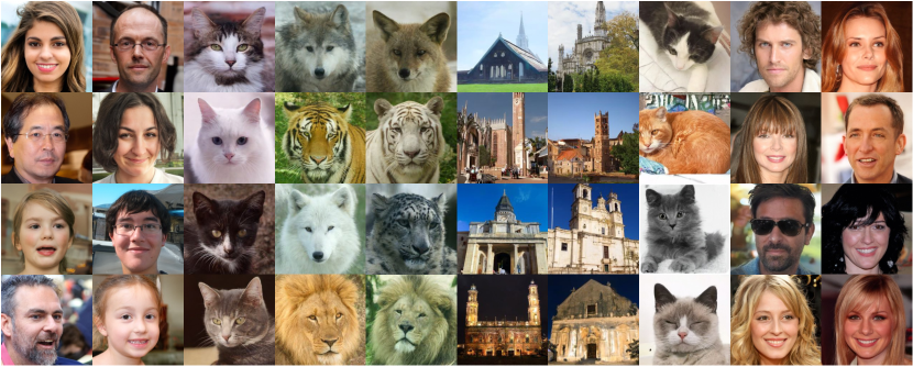
Figure 4: Qualitative results produced by E-TSDM on various datasets, including FFHQ $256\times 256$ [13], AFHQ-Cat $256\times 256$ [6], AFHQ-Wild $256\times 256$ [6], Lsun-Church $256\times 256$ [33], Lsun-Cat $256\times 256$ [33], CelebAHQ $256\times 256$ [12].

In this section, we present compelling evidence that our E-TSDM outperforms existing approaches on a variety of datasets. To achieve this, we first detail the experimental setup used in our studies in Sec. 5.1. Subsequently, in Sec. 5.2, we compare the synthesis performance of E-TSDM against that of the baseline on various datasets. Remarkably, our approach sets a new state-of-the-art benchmark for diffusion models on FFHQ $256\times 256$ [13]. In Sec. 5.3, we conduct multiple ablation studies and quantitative analysis from two perspectives. Firstly, we demonstrate the generalizability of E-TSDM by implementing it in continuous-time diffusion models and changing the noise schedules. Secondly, we investigate the impact of changing the number of conditions $n$ in $t\in[0,\tilde{t})$ and the length of the interval $\tilde{t}$, which are important hyperparameters. Moreover, we demonstrate in Sec. 5.4 that our method can be effectively combined with popular fast sampling techniques. Finally, we show that E-TSDM can be applied to conditional generation tasks, such as super-resolution, in Sec. 5.5.

Table 1: Quantitative comparison on various datasets with $256\times 256$ resolution. All experiments are evaluated with FID-10k, where smaller number indicates better performance.

	DDPM [10]	E-TSDM
AFHQ-Cat  [6]	7.19	$\bf 6.63$
AFHQ-Wild  [6]	9.64	$\bf 7.34$
FFHQ  [13]	9.50	$\bf 6.62$
CelebAHQ  [12]	8.05	$\bf 6.99$
Lsun-Church  [33]	7.01	$\bf 6.72$
Lsun-Cat  [33]	14.69	$\bf 11.98$

Table 2: Quantitative comparison on FFHQ [13]. $\ast$ denotes our reproduced result using the same network as our E-TSDM-large.

Model	FID-50k $\downarrow$
StyleGAN2$+$ADA$+$bCR [14]	3.62
Soft-Truncation [16]	5.54
P2-DM [5]	6.92
LDM [24]	4.98
DDPM [10]	6.88∗
E-TSDM (ours)	5.21
E-TSDM-large (ours)	4.22

5.1 Experimental setup

Implementation details. All of our experiments utilize the settings of DDPM [10] (see more details in Supplementary Material). Besides, we utilize a more developed structure of unet [7] than that of DDPM [10] for all experiments containing reproduced baseline. To ensure fairness, we reproduce the baseline on all datasets using the same network structure. Given that the model size is kept constant, the speed and memory requirements for training and inference for both the baseline and E-TSDM are the same. Except for the ablation studies in Sec. 5.3, all other experiments fix $\tilde{t}=100$ for E-TSDM and use five conditions ($n=5$) in the interval $t\in[0,\tilde{t})$, which we have found to be a relatively good choice in practice. Furthermore, all experiments are trained on NVIDIA A100 GPUs.

Datasets We implement E-TSDM on several widely evaluated datasets including FFHQ $256\times 256$ [13], CelebAHQ $256\times 256$ [12], AFHQ-Cat $256\times 256$ [6], AFHQ-Wild $256\times 256$ [6], Lsun-Church $256\times 256$ [33], Lsun-Cat $256\times 256$ [33].

Evaluation metrics. In order to assess the sampling quality of E-TSDM, we utilize the widely-adopted Frechet inception distance (FID) metric [9]. Additionally, we use the peak signal-to-noise ratio (PSNR) to evaluate the performance of the super-resolution task. To be more specific, we calculate FID using 10,000 samples for all of our experiments.

5.2 Synthesis performance

We have demonstrated that E-TSDM can effectively mitigate the large Lipschitz constants near $t=0$ in Fig. 1 b, as detailed in Sec. 4. In this section, we show that E-TSDM can improve the synthesis performance. To this end, we conduct a comprehensive comparison between E-TSDM and the DDPM baseline [10] on various datasets. The quantitative comparison between DDPM and E-TSDM is presented in Tab. 2, which clearly illustrates that E-TSDM outperforms the baseline on all evaluated datasets. Furthermore, as depicted in Fig. 4, the samples generated by E-TSDM on various datasets demonstrate its ability to generate high-fidelity images. Remarkably, to the best of our knowledge, as shown in Tab. 2, we set a new state-of-the-art benchmark for diffusion models on FFHQ $256\times 256$ [13] using a large version of our approach (see details in Supplementary Material).

5.3 Ablation study and quantitative analysis

In this section, we design several analytic experiments to demonstrate the generalizability of E-TSDM by implementing it on continuous-time diffusion models and changing the noise schedules. In addition, in order to gain a deeper understanding of the properties of E-TSDM, we conduct ablation studies to investigate the critical hyperparameters of E-TSDM, namely the number of conditions $n$ and the length of the interval $\tilde{t}$ to share the timestep conditions.

Table 3: Quantitative comparison between DDPM baseline [10] and our proposed E-TSDM on the generalized scenarios, on FFHQ $256\times 256$ [13] using FID-10k $\downarrow$ as the evaluation metric. Specifically, one scenario is to vary the noise schedule from the linear schedule to the popular quadratic schedule, the other scenario is to implement E-TSDM on the continuous-time diffusion models. Experimental results illustrate that E-TSDM can be generalized to other noise schedules and is still effective in the context of continuous-time diffusion models.

Settings	Method	FID $\downarrow$	Settings	Method	FID $\downarrow$
Discrete	DDPM [10]	13.79	Continuous	DDPM [10]	9.53
$+$ Quadratic	E-TSDM	$\bf 9.69$	$+$ Linear	E-TSDM	$\bf 6.95$

5.3.1 Quantitative analysis on the generalizability of E-TSDM

To ensure the generalizability of E-TSDM beyond specific settings of DDPM [10], we conduct a thorough investigation of E-TSDM on another popular noise schedule, as well as implement a continuous-time version of E-TSDM. Regarding the noise schedule, there are several popular options including linear, quadratic, and cosine schedules. However, the cosine schedule adds too little noise to fully destroy high-resolution images ($256\times 256$), resulting in poor performance [4, 11]. Therefore, we only consider the quadratic schedule as a supplement to the linear schedule. Moreover, we implement E-TSDM in the continuous-time diffusion models, which have received increasing attention recently [31, 15], and reproduce its corresponding baseline.

As shown in Tab. 3, our E-TSDM achieves excellent performance across different noise schedules, highlighting its effects independently of the specific noise schedule. Additionally, the continuous-time version of E-TSDM outperforms the corresponding baseline, indicating that E-TSDM is effective for both continuous-time and discrete-time diffusion models. We provide the curves of the Lipschitz constants $K(t,t^{\prime})$ in Fig. 3 for both continuous-time E-TSDM and its baseline, showing the ability of E-TSDM to eliminate Lipschitz singularities in the continuous-time scenario (see $K(t,t^{\prime})$ for quadratic schedule in Supplementary Material).

\begin{overpic}[width=429.28616pt]{figures/ab.pdf} \put(18.0,-1.0){(a) Timestep Number} \put(68.0,-1.0){(b) Interval Length} \put(1.5,15.0){\rotatebox{90.0}{FID-10K}} \end{overpic}

Figure 5: Ablation study on the length of the interval $t\in[0,\tilde{t})$ to share the timestep conditions $\tilde{t}$, and the number of timestep conditions in this interval $n$, using FID-10k $\downarrow$ as the evaluation metric.

5.3.2 The number of timestep conditions

E-TSDM involves dividing the target interval with large Lipschitz constants into $n$ sub-intervals and sharing timestep conditions within each sub-interval. Accordingly, the choice of $n$ has a significant impact on the performance of E-TSDM. Intuitively, $n$ should not be too large or too small. If $n$ is too small, the operation of sharing conditions may weaken the network’s ability, leading to a potential decline in performance. Conversely, if the value of $n$ is set too large, the number of boundaries of the sub-intervals increases. While E-TSDM enforces zero Lipschitz constants within each sub-interval, the timesteps near the boundaries have a non-zero Lipschitz constant. Therefore, a large number of sub-intervals may lead to an insufficient reduction in the overall Lipschitz constants of the target interval.

We conduct an in-depth evaluation of the impact of $n$ on FFHQ $256\times 256$ in this section. As shown in Fig. 5 a, we observe a rise in FID when $n$ is too small, for instance, when $n=2$. Conversely, when $n$ is too large, such as $n=100$, the performance deteriorates significantly. Although E-TSDM performs well on FFHQ $256\times 256$ for most $n$, we take into consideration the results on other datasets (see more results on other datasets in Supplementary Material) to make a general recommendation. We suggest using a relatively but not excessively small value of $n$, such as the default value of $n=5$ when applying E-TSDM without a thorough search.

Recall the observation that Lipschitz constants tend to be high around $t=0$, which is also a common symptom of overfitting. Besides, we can view the operation of sharing conditions in E-TSDM as reducing the number of degrees of freedom. By implementing this strategy, we significantly reduce the Lipschitz constants, thereby mitigating the issue of overfitting. Based on these findings, we can reasonably infer that traditional diffusion models are probably overfitted near zero.

Table 4: Quantitative comparison on FFHQ $256\times 256$ [13] between DDPM [10] and our proposed E-TSDM utilizing different fast samplers, DDIM [27] and DPM-Solver [19], varying the number of function evalutaions (NFE). FID-10k is used as the evaluation metric, and DPM-Solver-$k$ represents the $k$-th-order DPM-Solver. Results indicate that our approach well supports the popular fast samplers.

Sampling Method	NFE	Method	FID $\downarrow$
DPM-Solver-3 [19]	20	DDPM [10]	21.91
		E-TSDM	$\bf 16.97$
	50	DDPM [10]	24.48
		E-TSDM	$\bf 13.52$
DPM-Solver-2 [19]	20	DDPM [10]	22.21
		E-TSDM	$\bf 17.28$
	50	DDPM [10]	24.80
		E-TSDM	$\bf 14.14$
DDIM [27]	50	DDPM [10]	21.80
		E-TSDM	$\bf 19.34$
	200	DDPM [10]	23.16
		E-TSDM	$\bf 13.71$

5.3.3 The length of the interval to share condition

We claim that the large Lipschitz constants arise in diffusion models when the noise level is low, and our proposed E-TSDM shares condition in the interval $t\in[0,\tilde{t})$, where $\tilde{t}$ is a small threshold and its selection is critical to the performance of E-TSDM. In this section, we investigate the impact of $\tilde{t}$ on AFHQ-Cat $256\times 256$ [6] by varying $\tilde{t}$ (see more results on other datasets in Supplementary Material). Note that as $n$ is defined as the number of conditions in the interval $t\in[0,\tilde{t})$, it should increase proportionally with $\tilde{t}$. For instance, the default settings are $\tilde{t}=100$ and $n=5$, meaning that each timestep condition covers 20 noise levels. In this ablation study, we maintain the number of corresponding noise levels for each condition unchanged. Thus, when $\tilde{t}$ is set to 200, $n$ should be 10.

The results presented in Fig. 5 b demonstrate that E-TSDM performs well when $\tilde{t}$ is relatively small. However, as $\tilde{t}$ increases beyond a certain threshold, the performance of E-TSDM deteriorates significantly. Despite the presence of some outliers, the default value of $\tilde{t}=100$ consistently performs well across all evaluated datasets as in Tab. 2, which is recommended when applying E-TSDM without a thorough search.

5.4 Fast sampling

With the development of fast sampling algorithms, it is crucial that E-TSDM can be effectively combined with popular fast samplers, such as DDIM [27] and DPM-Solver [19]. To this end, we incorporate both DDIM [27] and DPM-Solver [19] into E-TSDM for fast sampling in this section. It should be noted that large Lipschitz constants can impede fast sampling more than full-timestep sampling. Because numerical solvers typically rely on the similarity of function values and their derivatives on adjacent steps, large discretization steps in fast sampling algorithms require greater smoothness, which corresponds to smaller Lipschitz constants. Consequently, we expect that E-TSDM will enhance the generation performance of fast sampling methods.

As presented in Tab. 4, we observe that E-TSDM significantly outperforms the baseline when using the same strategy for fast sampling, which is under expectation. As seen in Tab. 4, the advantage of E-TSDM becomes more pronounced when using higher order sampler (from DDIM [27] to DPM-Solver [19]), indicating better smoothness when compared to the baseline. Notably, for both DDIM [27] and DPM-Solver [19], we observe an abnormal phenomenon for baseline, whereby the performance deteriorates as the number of function evaluations (NFE) increases. This phenomenon has been previously noted by several works [19, 20, 17], but remains unexplained. Given this phenomenon is not observed in E-TSDM, we hypothesize that it may be related to the smoothness of the learned network. We leave further verification of this hypothesis for future work.

\begin{overpic}[width=433.62pt]{figures/super_resolution_compare.pdf} \put(-2.0,32.0){Low resolution} \put(-0.5,23.0){Original one} \put(1.0,14.5){Baseline} \put(-1.0,12.0){PSNR$\uparrow$: 24.64} \put(2.0,4.5){Ours} \put(-1.0,2.0){PSNR$\uparrow$: 25.61} \end{overpic}

Figure 6: Qualitative and quantitative results by applying E-TSDM to super-resolution task (i.e., from $64\times 64$ to $256\times 256$), using PSNR as the evaluation metric. Results show that E-TSDM mitigates the color bias occurring in baseline and improves the PSNR from 24.64 to 25.61, which suggests that our approach well supports conditional generation.

5.5 Conditional generation

We have demonstrated the efficiency of E-TSDM in the context of unconditional generation tasks. In order to explore the potential for extending E-TSDM to conditional generation tasks, we further investigate its performance in the super-resolution task, which is one of the most popular conditional generation tasks. Specifically, we test E-TSDM on the FFHQ $256\times 256$ dataset, using the $64\times 64\rightarrow 256\times 256$ pixel resolution as our experimental settings. For the baseline in the super-resolution task, we utilize the same network structure and hyper-parameters as those employed in the baseline presented in Sec. 5.1, but incorporate a low-resolution image as an additional input. Besides, for E-TSDM, we adopt a general setting with $n=5$ and $\tilde{t}=100$.

As illustrated in Fig. 6, we observe that the baseline tends to exhibit a color bias compared to real images, which is mitigated by E-TSDM. Quantitatively, our results indicate that E-TSDM outperforms the baseline on the test set, achieving an improvement in PSNR from 24.64 to 25.61. These findings suggest that E-TSDM holds considerable promise for application in conditional generation tasks.

6 Conclusion

In this paper, we have elaborated on the infinite Lipschitz of the diffusion model near the zero point from both theoretical and empirical perspectives, which wreaks havoc on the stability and accuracy of the diffusion process. A novel E-TSDM is further proposed to eliminate the corresponding singularity in a timestep-sharing manner. Experimental results demonstrate the superiority of our method in both performance and adaptability to the baselines, including unconditional generation, conditional generation, and fast sampling.

Limitations Although E-TSDM has demonstrated significant improvements in various applications, it has yet to be verified on large-scale text-to-image generative models. As E-TSDM reduces the large Lipschitz constants by sharing conditions, there is a possibility that this may lead to a decrease in the effectiveness of large-scale generative models. Additionally, the reduction of Lipschitz constants to zero within each sub-interval in E-TSDM may introduce unknown and potentially harmful effects.

Appendix

Overview

This supplementary material is organized as follows. First, to facilitate the reproducibility of our experiments, we present implementation details, including hyper-parameters in Sec. A.1 and algorithmic details in Sec. A.2. Next, in appendix B, we provide all details of deduction involved in the main paper. Finally, we present additional experimental results in support of the effectiveness of E-TSDM.

Appendix A Implementation details

A.1 Hyper-parameters

The hyper-parameters used in our experiments are shown in Tab. 5, and we use identical hyper-parameters for all evaluated datasets for both E-TSDM and their corresponding baselines. Specifically, we follow the hyper-parameters of DDPM [10] but adopt a more advanced structure of U-Net [7] with residual blocks from BigGAN [3]. The network employs a block consisting of fully connected layers to encode the timestep, where the dimensionality of hidden layers for this block is determined by the timestep channels shown in Tab. 5.

Table 5: Hyper-parameters of E-TSDM and our reproduced baseline.

	Normal version	Large version
$T$	1,000	1,000
$\beta_{t}$	linear	linear
Model size	131M	692M
Base channels	128	128
Channels multiple	(1,1,2,2,4,4)	(1,1,2,4,6,8)
Heads channels	64	64
Self attention	32,16,8	32,64,8
Timestep channels	512	2048
BigGAN block	✓	✓
Dropout	0.0	0.0
Learning rate	1e-4	1e-4
Batch size	96	64
Res blocks	2	4
EMA	0.9999	0.9999
Warmup steps	0	0
Gradient clip	✗	✗

Moreover, we scale up the network to achieve the state-of-the-art results of diffusion models on FFHQ $256\times 256$ [13], and therefore we provide the hyper-parameters of the large version of E-TSDM in Tab. 5.

A.2 Algorithm details

In this section, we provide a detailed description of the E-TSDM algorithm, including the training and inference procedures as shown in algorithm 1 and algorithm 2, respectively. Our method is simple to implement and requires only a few steps. Firstly, a suitable length of the interval $\tilde{t}$ should be selected for sharing conditions, along with the corresponding number of timestep conditions $n$ in the target interval $t\in[0,\tilde{t})$. While performing a thorough search for different datasets can achieve better performance, the default settings $\tilde{t}=100$ and $n=5$ are recommended when E-TSDM is applied without a thorough search.

Algorithm 1 Training of E-TSDM

1:The length of the target interval $\tilde{t}$.

2:The number of conditions $n$.

3:Model ${\mathbf{\epsilon}}_{\theta}$ to be trained.

4:Data set $\mathcal{D}$.

5:Uniformly divide the target interval $t\in[0,\tilde{t})$ into $n$ sub-intervals to get the corresponding timestep partition schedule ${\mathbb{T}}=\{t_{0},t_{1},\dots,t_{n}\}$.

6:repeat

7:     ${\mathbf{x}}_{0}\sim\mathcal{D}$

8:     $t\sim\text{Uniform}(\{1,\dots,T\})$

9:     if $t<\tilde{t}$ then

10:         $\hat{t}=\max_{1\leq i\leq n}\{t_{i-1}\in{\mathbb{T}}:t_{i-1}\leq t\}$

11:     else

12:         $\hat{t}=t$

13:     end if

14:     $\epsilon\sim\mathcal{N}(\mathbf{0},\mathbf{I})$

15:     Take gradient descent step on

16:   $\nabla_{\theta}\|{\mathbf{\epsilon}}-{\mathbf{\epsilon}}_{\theta}(\alpha_{t}{\mathbf{x}}_{0}+\sigma_{t}{\mathbf{\epsilon}},\hat{t})\|^{2}$

17:until converged

Algorithm 2 Sampling of E-TSDM

1:The length of the target interval $\tilde{t}$.

2:The number of conditions $n$.

3:A trained model ${\mathbf{\epsilon}}_{\theta}$.

4:Uniformly divide the target interval $t\in[0,\tilde{t})$ into $n$ sub-intervals to get the corresponding timestep partition schedule ${\mathbb{T}}=\{t_{0},t_{1},\dots,t_{n}\}$.

5:${\mathbf{x}}_{T}\sim\mathcal{N}(\mathbf{0},\mathbf{I})$

6:for $t=T,\dots,1$ do

7:     if $t<\tilde{t}$ then

8:         $\hat{t}=\max_{1\leq i\leq n}\{t_{i-1}\in{\mathbb{T}}:t_{i-1}\leq t\}$

9:     else

10:         $\hat{t}=t$

11:     end if

12:     if $t>1$ then

13:         ${\mathbf{z}}\sim\mathcal{N}(\mathbf{0},\mathbf{I})$

14:     else

15:         ${\mathbf{z}}=0$

16:     end if

17:     ${\mathbf{x}}_{t-1}=\frac{\alpha_{t-1}}{\alpha_{t}}\left({\mathbf{x}}_{t}-\frac{\beta_{t}}{\sigma_{t}}{\mathbf{\epsilon}}_{\theta}({\mathbf{x}}_{t},\hat{t})\right)+\eta_{t}{\mathbf{z}}$

18:end for

19:return ${\mathbf{x}}_{0}$

Next, the target interval $t\in[0,\tilde{t})$ should be divided into $n$ sub-intervals, and the boundaries for each sub-interval should be calculated to generate the partition schedule ${\mathbb{T}}=\{t_{0},t_{1},\dots,t_{n}\}$. Finally, during both training and sampling, the corresponding left boundary $\hat{t}$ for each timestep in the target interval $t\in[0,\tilde{t})$ should be determined according to ${\mathbb{T}}$, and used as the conditional input of the network instead of $t$.

Appendix B Derivation of formulas

We have already shown that for an arbitrary complex distribution, given a noise schedule, if $\left.\frac{{\rm d}\alpha_{t}}{{\rm d}t}\right|_{t=0}\neq 0$, then we often have $\lim\sup_{t\rightarrow 0+}\big{\lVert}\frac{\partial\epsilon_{\theta}({\mathbf{x}},t)}{\partial t}\big{\rVert}\rightarrow\infty$, indicating the infinite Lipschitz constants around $t=0$. In this section, we prove that $\left.\frac{{\rm d}\alpha_{t}}{{\rm d}t}\right|_{t=0}\neq 0$ stands for three mainstream noise schedules including linear schedule, quadratic schedule and cosine schedule.

B.1 ${\rm d}\alpha_{t}/{\rm d}t$ for linear and quadratic schedules at zero point

Linear and quadratic schedules are first proposed by [10]. Both of them determine $\{\alpha_{t}\}_{t=1}^{T}$ by a pre-designed positive sequence $\{\beta_{t}\}_{t=1}^{T}$ and the relationship $\alpha_{t}:=\prod_{i=1}^{t}\sqrt{1-\beta_{i}}$. Note that $t\in\{1,2,\cdots,T\}$ is a discrete index, and $\{\alpha_{t}\}_{t=1}^{T}$, $\{\beta_{t}\}_{t=1}^{T}$ are discrete parameter sequences in DDPM. However, $\alpha_{t}$ in ${\rm d}\alpha_{t}/{\rm d}t$ actually refers to the continuous-time parameter determined by the following score SDE [31]

$${\rm d}{\mathbf{x}}(\tau)=-\frac{1}{2}\beta(\tau){\mathbf{x}}(\tau){\rm d}\tau+\sqrt{\beta(\tau)}{\rm d}{\mathbf{w}},~{}\tau\in[0,1],$$ (10)

where ${\mathbf{w}}$ is the standard Wiener process, $\beta(\tau)$ is the continuous version of $\{\beta_{t}\}_{t=1}^{T}$ with a continuous time variable $\tau\in[0,1]$ for indexing, and the continuous-time $\alpha_{t}=\exp{(-\frac{1}{2}\int_{0}^{t}\beta(s){\rm d}s)}$. To avoid ambiguity, let $\alpha(\tau),~{}\tau\in[0,1]$ denote the continuous version of $\{\alpha_{t}\}_{t=1}^{T}$. Thus,

$$\left.\frac{{\rm d}\alpha(\tau)}{{\rm d}\tau}\right|_{\tau=0}=\left.-\frac{1}{2}\beta(\tau)\exp{(-\frac{1}{2}\int_{0}^{\tau}\beta(s){\rm d}s)}\right|_{\tau=0}=-\frac{1}{2}\beta(0).$$ (11)

Once the continuous function $\beta(\tau)$ is determined for a specific noise schedule, we can obtain $\left.\frac{{\rm d}\alpha(\tau)}{{\rm d}\tau}\right|_{\tau=0}$ immediately by Eq. 11.

To obtain $\beta(\tau)$, we first give the expression of $\{\beta_{t}\}_{t=1}^{T}$ in linear and quadratic schedules [10]

Linear: $$\beta_{t}=\frac{\bar{\beta}_{\rm min}}{T}+\left(\frac{\bar{\beta}_{\rm max}}{T}-\frac{\bar{\beta}_{\rm min}}{T}\right)\cdot\frac{t-1}{T-1},$$ (12)

Quadratic: $$\beta_{t}=\left(\sqrt{\frac{\bar{\beta}_{\rm min}}{T}}+\left(\sqrt{\frac{\bar{\beta}_{\rm max}}{T}}-\sqrt{\frac{\bar{\beta}_{\rm min}}{T}}\right)\cdot\frac{t-1}{T-1}\right)^{2},$$ (13)

where $\bar{\beta}_{\rm min}$ and $\bar{\beta}_{\rm max}$ are user-defined hyperparameters. Then, we define an auxiliary sequence $\{\bar{\beta}_{t}=T\beta_{t}\}_{t=1}^{T}$. In the limit of $T\rightarrow\infty$, $\{\bar{\beta}_{t}\}_{t=1}^{T}$ becomes the function $\beta(\tau)$ indexed by $\tau\in[0,1]$

Linear: $$\beta(\tau)=\bar{\beta}_{\rm min}+\left(\bar{\beta}_{\rm max}-\bar{\beta}_{\rm min}\right)\cdot\tau,$$ (14)

Quadratic: $$\beta(\tau)=\left(\sqrt{\bar{\beta}_{\rm min}}+\left(\sqrt{\bar{\beta}_{\rm max}}-\sqrt{\bar{\beta}_{\rm min}}\right)\cdot\tau\right)^{2},$$ (15)

Thus, $\beta(0)=\bar{\beta}_{\rm min}$ for both linear and quadratic schedules, which leads to $\left.\frac{{\rm d}\alpha(\tau)}{{\rm d}\tau}\right|_{\tau=0}=-\frac{1}{2}\bar{\beta}_{\rm min}$. As a common setting, $\bar{\beta}_{\rm min}$ is a positive real number, thus $\left.\frac{{\rm d}\alpha(\tau)}{{\rm d}\tau}\right|_{\tau=0}<0$.

B.2 ${\rm d}\alpha_{t}/{\rm d}t$ for cosine schedule at zero point

Cosine schedule is designed to prevent abrupt changes in noise level near $t=0$ and $t=T$ [21]. Different from linear and quadratic schedules that define $\{\alpha_{t}\}_{t=1}^{T}$ by a pre-degined sequence $\{\beta_{t}\}_{t=1}^{T}$, cosine schedule directly defines $\{\alpha_{t}\}_{t=1}^{T}$ as

$$\alpha_{t}=\frac{f(t)}{f(0)},\quad f(t)=\cos{\left(\frac{t/T+s}{1+s}\cdot\frac{\pi}{2}\right)},\quad t=1,2,\cdots,T,$$ (16)

where $s$ is a small positive offset. The continuous version of $\{\alpha_{t}\}_{t=1}^{T}$ can be obtained in the limit of $T\rightarrow\infty$ as

$$\alpha(\tau)=\cos{\left(\frac{\tau+s}{1+s}\cdot\frac{\pi}{2}\right)}/\cos{\left(\frac{s}{1+s}\cdot\frac{\pi}{2}\right)},\quad\tau\in[0,1].$$ (17)

With Eq. 17, we can easily get $\left.\frac{{\rm d}\alpha(\tau)}{{\rm d}\tau}\right|_{\tau=0}$

$$\left.\frac{{\rm d}\alpha(\tau)}{{\rm d}\tau}\right|_{\tau=0}=-\frac{\pi}{2(1+s)}\tan{\left(\frac{s}{1+s}\cdot\frac{\pi}{2}\right)},$$ (18)

which leads to $\left.\frac{{\rm d}\alpha(\tau)}{{\rm d}\tau}\right|_{\tau=0}<0$ since $s>0$.

\begin{overpic}[width=429.28616pt]{figures/lipschitz_constants_.pdf} \put(14.0,68.0){(a) AFHQ-Cat $256\times 256$} \put(24.5,70.5){100} \put(8.5,70.5){0} \put(38.0,70.5){1000} \put(6.0,73.0){0} \put(5.2,98.0){24} \put(5.5,78.0){\rotatebox{90.0}{Lipschitz Constants}} \par\put(58.0,68.0){(b) AFHQ-Wild $256\times 256$} \put(69.0,70.5){100} \put(53.0,70.5){0} \put(82.5,70.5){1000} \put(50.5,73.0){0} \put(49.7,98.0){24} \put(50.0,78.0){\rotatebox{90.0}{Lipschitz Constants}} \par\put(15.0,31.5){(c) Lsun-Cat $256\times 256$} \put(24.5,34.0){100} \put(8.5,34.0){0} \put(38.0,34.0){1000} \put(6.0,36.5){0} \put(5.2,61.5){24} \put(5.5,41.5){\rotatebox{90.0}{Lipschitz Constants}} \par\put(58.0,31.5){(d) Lsun-Church $256\times 256$} \put(69.0,34.0){100} \put(53.0,34.0){0} \put(82.5,34.0){1000} \put(50.5,36.5){0} \put(49.7,61.5){24} \put(50.0,41.5){\rotatebox{90.0}{Lipschitz Constants}} \par\put(14.0,-5.0){(e) CelebAHQ $256\times 256$} \put(24.5,-2.5){100} \put(8.5,-2.5){0} \put(38.0,-2.5){1000} \put(6.0,0.0){0} \put(5.2,25.0){24} \put(5.5,5.0){\rotatebox{90.0}{Lipschitz Constants}} \par\put(58.0,-5.0){(f) FFHQ $256\times 256$ using} \put(62.0,-7.5){quadratic schedule} \put(69.0,-2.5){100} \put(53.0,-2.5){0} \put(82.5,-2.5){1000} \put(50.5,0.0){0} \put(49.7,25.0){24} \put(50.0,5.0){\rotatebox{90.0}{Lipschitz Constants}} \end{overpic}

Figure 7: Quantitative comparison of Lipschitz constants between E-TSDM and DDPM baseline [10] on various datasets, including (a) AFHQ-Cat [6], (b) AFHQ-Wild [6], (c) Lsun-Cat $256\times 256$ [13], (d) Lsun-Church $256\times 256$ [13], and (e) CelebAHQ $256\times 256$ [12] using linear schedule. (f) Quantitative comparison of Lipschitz constants between E-TSDM and DDPM baseline [10] on FFHQ $256\times 256$ [13] using quadratic schedule.

\begin{overpic}[width=429.28616pt]{figures/ablation_t_supp.pdf} \put(16.0,34.5){(a) FFHQ $256\times 256$} \put(20.0,38.0){Interval Length} \put(1.0,52.0){\rotatebox{90.0}{FID-10k}} \par\put(65.0,34.5){(b) CelebAHQ $256\times 256$} \put(72.0,38.0){Interval Length} \put(52.0,52.0){\rotatebox{90.0}{FID-10k}} \par\put(14.0,-6.0){(c) LSUN-Cat $256\times 256$} \put(20.0,-2.5){Interval Length} \put(1.0,11.0){\rotatebox{90.0}{FID-10k}} \par\put(65.0,-6.0){(d) LSUN-Church $256\times 256$} \put(72.0,-2.5){Interval Length} \put(52.0,11.0){\rotatebox{90.0}{FID-10k}} \end{overpic}

Figure 8: Ablation study on the length of the interval $t\in[0,\tilde{t})$ to share the timestep conditions, $\tilde{t}$, using FID-10k $\downarrow$ as the evaluation metric.

\begin{overpic}[width=429.28616pt]{figures/ablation_n_supp.pdf} \put(16.0,33.5){(a) CelebAHQ $256\times 256$} \put(20.0,37.0){Timestep Number} \put(2.0,52.0){\rotatebox{90.0}{FID-10k}} \par\put(65.0,33.5){(b) AFHQ-Cat $256\times 256$} \put(72.0,37.0){Timestep Number} \put(53.0,52.0){\rotatebox{90.0}{FID-10k}} \par\put(14.0,-6.0){(c) LSUN-Cat $256\times 256$} \put(20.0,-2.5){Timestep Number} \put(2.0,11.0){\rotatebox{90.0}{FID-10k}} \par\put(65.0,-6.0){(d) LSUN-Church $256\times 256$} \put(72.0,-2.5){Timestep Number} \put(53.0,11.0){\rotatebox{90.0}{FID-10k}} \end{overpic}

Figure 9: Ablation study on the number of timestep conditions in this interval, $n$, using FID-10k $\downarrow$ as the evaluation metric.

Appendix C Additional results

C.1 Lipschitz constants

In our main paper, we demonstrate the effectiveness of E-TSDM in reducing the Lipschitz constants near $t=0$ by comparing its Lipschitz constants with that of DDPM baseline [10] on the FFHQ $256\times 256$ dataset [13]. As a supplement, we provide additional comparisons of Lipschitz constants on other datasets, including AFHQ-Cat [6] (see Fig. 7a), AFHQ-Wild [6] (see Fig. 7b), Lsun-Cat $256\times 256$ [13] (see Fig. 7c), Lsun-Church $256\times 256$ [13] (see Fig. 7d), and CelebAHQ $256\times 256$ [12] (see Fig. 7e). These experimental results demonstrate that E-TSDM is highly effective in eliminating Lipschitz singularities in diffusion models across various datasets.

Furthermore, we provide a comparison of Lipschitz constants between E-TSDM and the DDPM baseline [10] when using a quadratic schedule. As shown in Fig. 7f, we observe that large Lipschitz constants still exist in diffusion models when using a quadratic schedule. However, E-TSDM effectively eliminates this problem, highlighting the superiority of our approach over the DDPM baseline.

C.2 Quantitative analysis and ablation studies

C.2.1 The length of interval to share condition $\tilde{t}$ and the number of conditions $n$

In our main paper, we investigated the impact of two important settings for E-TSDM, the length of the interval to share conditions $\tilde{t}$, and the number of timestep conditions $n$ in this interval. As a supplement, we provide additional results on various datasets to further investigate the optimal settings for these parameters.

As seen in Fig. 8 and Fig. 9, we observe divergence in the best choices of $n$ and $\tilde{t}$ across different datasets. However, we find that the default settings where $\tilde{t}=100$ and $n=5$ consistently yield good performance across a range of datasets. Based on these findings, we recommend the default settings as an ideal choice for implementing E-TSDM without the need for a thorough search. However, if performance is the main concern, researchers may conduct a grid search to explore the optimal values of $\tilde{t}$ and $n$ for specific dataset.

C.2.2 The noise schedule

In our main paper, we predominantly use the linear schedule, which is widely adopted in diffusion models. Moreover, we explore the effectiveness of E-TSDM on other noise schedules by utilizing the quadratic schedule. We abandon the cosine schedule as it adds too little noise on images to fully destroy data, resulting in poor performance [11]. However, Hoogeboom et al. [11] have recently proposed a new noise schedule that essentially replicates the design of the cosine schedule but yields a higher noise-to-signal ratio, which is called cosine-shift schedule in this paper. In other words, the cosine-shift schedule can add enough noise to images, thereby improving the synthesis performance In this section, we investigate the effectiveness of E-TSDM on cosine-shift schedule as a supplement to the main paper. As shown in Fig. 11, E-TSDM is also effective on the cosine-shift schedule, as it significantly reduces the Lipschitz constants and improves the FID-10k from 14.51 to 11.20.

\begin{overpic}[width=429.28616pt]{figures/lipschitz_constants_ffhq_cosine_shift.pdf} \put(45.0,-9.0){Timestep} \put(15.0,-4.0){0} \put(4.5,2.0){0} \put(4.5,62.0){12} \put(55.0,-4.0){100} \put(90.0,-4.0){1000} \put(4.5,11.0){\rotatebox{90.0}{Lipschitz Constants}} \end{overpic}

Figure 10: Quantitative comparison of Lipschitz constants between E-TSDM and DDPM baseline [10] on FFHQ $256\times 256$ [13] using cosine shift schedule.

\begin{overpic}[width=429.28616pt]{figures/lipschitz_constants_ffhq_difference.pdf} \put(45.0,-10.0){Timestep} \put(15.0,-5.0){0} \put(8.5,2.0){0} \put(8.5,62.0){24} \put(57.0,-5.0){100} \put(90.0,-5.0){1000} \put(8.5,11.0){\rotatebox{90.0}{Lipschitz Constants}} \end{overpic}

Figure 11: Quantitative comparison of Lipschitz constants among E-TSDM, DDPM [10], and DDPM [10] using regularization techniques (DDPM-r) on FFHQ $256\times 256$ [13].

C.3 Alternative methods

As mentioned in the main paper, one alternative method is to impose restrictions on the Lipschitz constants through regularization techniques. In this section, we apply regularization on baseline and estimate the gradient of $\epsilon_{\theta}({\mathbf{x}},t)$ by calculating the difference $K(t,t^{\prime})$. We represent this method as DDPM-r in this paper. As shown in Fig. 11, although DDPM-r can also reduce the Lipschitz constants, its capacity to do so is substantially inferior to that of E-TSDM. Additionally, DDPM-r necessitates twice the calculation compared to E-TSDM. Regarding synthesis performance, DDPM-r achieves a comparable FID-10k (7.97) with baseline (8.05), which is inferior to that of E-TSDM (6.99), indicating that E-TSDM is a better choice rather than regularization.

C.4 Latent diffusion models

Latent diffusion models (LDM) [24] is one of the most renowned variants of diffusion models. In this section, we will investigate the Lipschitz singularities in LDM [24], and apply E-TSDM to address this problem. LDM [24] shares a resemblance with DDPM [24] but has an additional auto-encoder to encode images into the latent space. As LDM typically employs the quadratic schedule, it is also susceptible to Lipschitz singularities, as confirmed in Fig. 13.

As seen in Fig. 13, by utilizing E-TSDM, the Lipschitz constants within each timestep-shared sub-interval are reduced to zero, while the timesteps located near the boundaries of the sub-intervals exhibit a Lipschitz constant comparable to that of baseline, leading to a decrease in overall Lipschitz constants in the target interval $t\in[0,\tilde{t})$, where $\tilde{t}$ is set as the default, namely $\tilde{t}=100$. Consequently, E-TSDM achieves an improvement in FID-50k from 4.98 to 4.61 with the adoption of E-TSDM, when $n=20$. We provide some samples generated by the E-TSDM implemented on LDM in Fig. 13.

\begin{overpic}[width=429.28616pt]{figures/lipschitz_constants_ffhq_ldm.pdf} \put(7.0,3.5){0} \put(12.0,-1.0){0} \put(7.0,62.0){6} \put(65.0,-1.0){100} \put(47.0,-6.0){Timestep} \put(88.0,-1.0){1000} \put(6.0,14.0){\rotatebox{90.0}{Lipschitz Constants}} \end{overpic}

Figure 12: Quantitative comparison of Lipschitz constants between E-TSDM and LDM [24] on FFHQ $256\times 256$[13]. E-TSDM reduces the overall Lipschitz constants near $t=0$, and eliminates the Lipschitz singularities occurring in LDM [24].

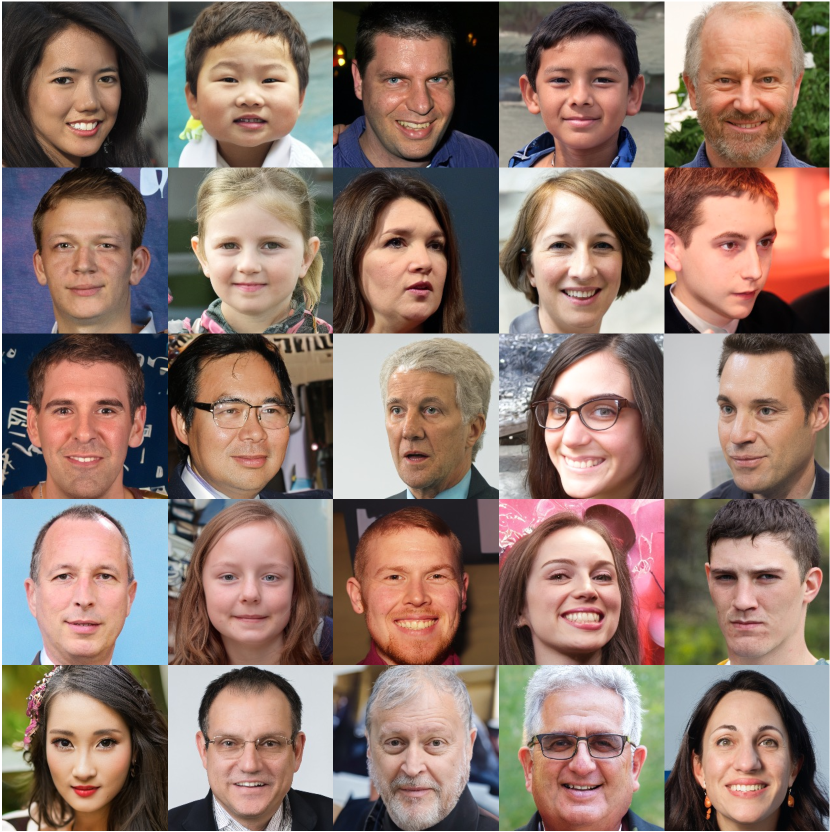
Figure 13: Qualitative results produced by E-TSDM implemented on LDM [24] on FFHQ $256\times 256$[13].

C.5 More samples

As a supplement, we provide more samples of E-TSDM trained on Lsun-Church $256\times 256$ [13] (see Fig. 14), Lsun-Cat $256\times 256$ [13] (see Fig. 15), AFHQ-Cat $256\times 256$ [6], AFHQ-Wild $256\times 256$ [6] (see Fig. 16), FFHQ $256\times 256$ [13] (see Fig. 17), and CelebAHQ $256\times 256$ [12] (see Fig. 18).

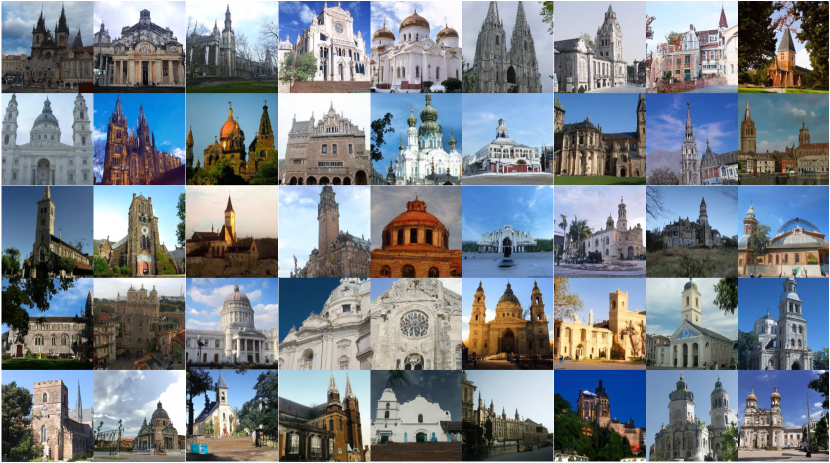
Figure 14: Qualitative results produced by E-TSDM on Lsun-Church $256\times 256$ [33].

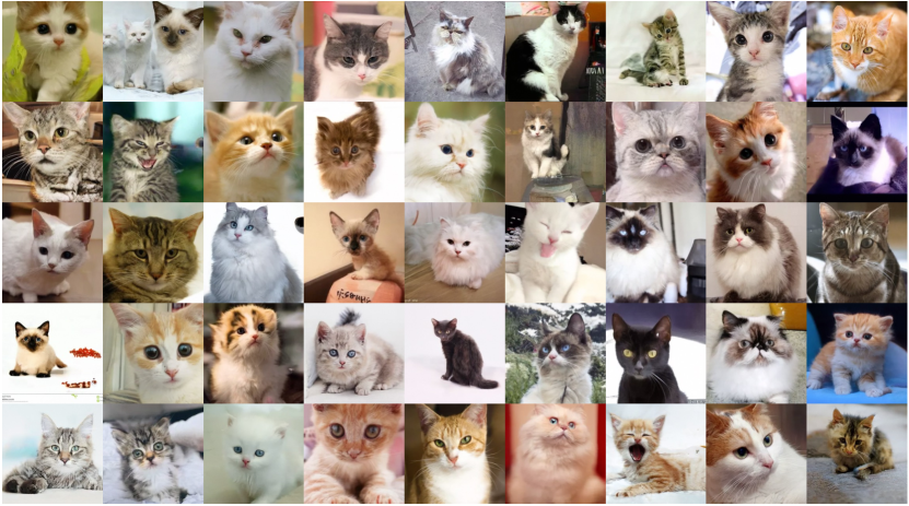
Figure 15: Qualitative results produced by E-TSDM on Lsun-Cat $256\times 256$ [33].

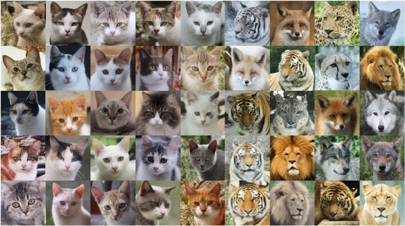
Figure 16: Qualitative results produced by E-TSDM on AFHQ-Cat $256\times 256$ [6] and AFHQ-Wild $256\times 256$ [6].

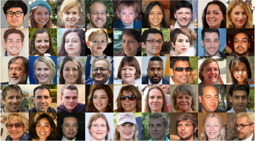
Figure 17: Qualitative results produced by E-TSDM on FFHQ $256\times 256$[13].

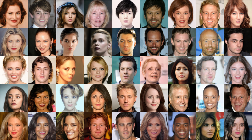
Figure 18: Qualitative results produced by E-TSDM on CelebAHQ $256\times 256$ [12].

References

- Bao et al. [2022a] F. Bao, C. Li, J. Sun, J. Zhu, and B. Zhang. Estimating the optimal covariance with imperfect mean in diffusion probabilistic models. arXiv preprint arXiv:2206.07309, 2022a.
- Bao et al. [2022b] F. Bao, C. Li, J. Zhu, and B. Zhang. Analytic-DPM: an analytic estimate of the optimal reverse variance in diffusion probabilistic models. arXiv preprint arXiv:2201.06503, 2022b.
- Brock et al. [2018] A. Brock, J. Donahue, and K. Simonyan. Large scale GAN training for high fidelity natural image synthesis. arXiv preprint arXiv:1809.11096, 2018.
- Chen [2023] T. Chen. On the importance of noise scheduling for diffusion models. arXiv preprint arXiv:2301.10972, 2023.
- Choi et al. [2022] J. Choi, J. Lee, C. Shin, S. Kim, H. Kim, and S. Yoon. Perception prioritized training of diffusion models. In IEEE Conf. Comput. Vis. Pattern Recog., pages 11472–11481, 2022.
- Choi et al. [2020] Y. Choi, Y. Uh, J. Yoo, and J.-W. Ha. StarGAN v2: Diverse image synthesis for multiple domains. In IEEE Conf. Comput. Vis. Pattern Recog., pages 8188–8197, 2020.
- Dhariwal and Nichol [2021] P. Dhariwal and A. Nichol. Diffusion models beat GANs on image synthesis. Adv. Neural Inform. Process. Syst., pages 8780–8794, 2021.
- Dockhorn et al. [2021] T. Dockhorn, A. Vahdat, and K. Kreis. Score-based generative modeling with critically-damped Langevin diffusion. arXiv preprint arXiv:2112.07068, 2021.
- Heusel et al. [2017] M. Heusel, H. Ramsauer, T. Unterthiner, B. Nessler, and S. Hochreiter. GANs trained by a two time-scale update rule converge to a local Nash equilibrium. Adv. Neural Inform. Process. Syst., 2017.
- Ho et al. [2020] J. Ho, A. Jain, and P. Abbeel. Denoising diffusion probabilistic models. In Adv. Neural Inform. Process. Syst., pages 6840–6851, 2020.
- Hoogeboom et al. [2023] E. Hoogeboom, J. Heek, and T. Salimans. Simple diffusion: End-to-end diffusion for high resolution images. arXiv preprint arXiv:2301.11093, 2023.
- Karras et al. [2017] T. Karras, T. Aila, S. Laine, and J. Lehtinen. Progressive growing of GANs for improved quality, stability, and variation. arXiv preprint arXiv:1710.10196, 2017.
- Karras et al. [2019] T. Karras, S. Laine, and T. Aila. A style-based generator architecture for generative adversarial networks. In IEEE Conf. Comput. Vis. Pattern Recog., pages 4401–4410, 2019.
- Karras et al. [2020] T. Karras, M. Aittala, J. Hellsten, S. Laine, J. Lehtinen, and T. Aila. Training generative adversarial networks with limited data. Adv. Neural Inform. Process. Syst., pages 12104–12114, 2020.
- Karras et al. [2022] T. Karras, M. Aittala, T. Aila, and S. Laine. Elucidating the design space of diffusion-based generative models. arXiv preprint arXiv:2206.00364, 2022.
- Kim et al. [2022] D. Kim, S. Shin, K. Song, W. Kang, and I.-C. Moon. Soft truncation: A universal training technique of score-based diffusion model for high precision score estimation. In Int. Conf. Mach. Learn., pages 11201–11228. PMLR, 2022.
- Li et al. [2023] S. Li, L. Liu, Z. Chai, R. Li, and X. Tan. Era-Solver: Error-Robust Adams solver for fast sampling of diffusion probabilistic models. arXiv preprint arXiv:2301.12935, 2023.
- Lu et al. [2022a] C. Lu, K. Zheng, F. Bao, J. Chen, C. Li, and J. Zhu. Maximum likelihood training for score-based diffusion odes by high order denoising score matching. In Int. Conf. Mach. Learn., pages 14429–14460. PMLR, 2022a.
- Lu et al. [2022b] C. Lu, Y. Zhou, F. Bao, J. Chen, C. Li, and J. Zhu. DPM-Solver: A fast ODE solver for diffusion probabilistic model sampling in around 10 steps. arXiv preprint arXiv:2206.00927, 2022b.
- Lu et al. [2022c] C. Lu, Y. Zhou, F. Bao, J. Chen, C. Li, and J. Zhu. Dpm-solver++: Fast solver for guided sampling of diffusion probabilistic models. arXiv preprint arXiv:2211.01095, 2022c.
- Nichol and Dhariwal [2021] A. Q. Nichol and P. Dhariwal. Improved denoising diffusion probabilistic models. In Int. Conf. Mach. Learn., pages 8162–8171, 2021.
- Pidstrigach [2022] J. Pidstrigach. Score-based generative models detect manifolds. In S. Koyejo, S. Mohamed, A. Agarwal, D. Belgrave, K. Cho, and A. Oh, editors, Adv. Neural Inform. Process. Syst., pages 35852–35865. Curran Associates, Inc., 2022.
- Ramesh et al. [2022] A. Ramesh, P. Dhariwal, A. Nichol, C. Chu, and M. Chen. Hierarchical text-conditional image generation with clip latents. arXiv preprint arXiv:2204.06125, 2022.
- Rombach et al. [2022] R. Rombach, A. Blattmann, D. Lorenz, P. Esser, and B. Ommer. High-resolution image synthesis with latent diffusion models. In IEEE Conf. Comput. Vis. Pattern Recog., pages 10684–10695, 2022.
- Saharia et al. [2022] C. Saharia, W. Chan, S. Saxena, L. Li, J. Whang, E. Denton, S. K. S. Ghasemipour, B. K. Ayan, S. S. Mahdavi, R. G. Lopes, et al. Photorealistic text-to-image diffusion models with deep language understanding. arXiv preprint arXiv:2205.11487, 2022.
- Sohl-Dickstein et al. [2015] J. Sohl-Dickstein, E. Weiss, N. Maheswaranathan, and S. Ganguli. Deep unsupervised learning using nonequilibrium thermodynamics. In Int. Conf. Mach. Learn., pages 2256–2265, 2015.
- Song et al. [2020] J. Song, C. Meng, and S. Ermon. Denoising diffusion implicit models. arXiv preprint arXiv:2010.02502, 2020.
- Song and Ermon [2019] Y. Song and S. Ermon. Generative modeling by estimating gradients of the data distribution. Adv. Neural Inform. Process. Syst., 2019.
- Song and Ermon [2020] Y. Song and S. Ermon. Improved techniques for training score-based generative models. Adv. Neural Inform. Process. Syst., pages 12438–12448, 2020.
- Song et al. [2021a] Y. Song, C. Durkan, I. Murray, and S. Ermon. Maximum likelihood training of score-based diffusion models. Adv. Neural Inform. Process. Syst., pages 1415–1428, 2021a.
- Song et al. [2021b] Y. Song, J. Sohl-Dickstein, D. P. Kingma, A. Kumar, S. Ermon, and B. Poole. Score-based generative modeling through stochastic differential equations. Int. Conf. Learn. Represent., 2021b.
- Vahdat et al. [2021] A. Vahdat, K. Kreis, and J. Kautz. Score-based generative modeling in latent space. Adv. Neural Inform. Process. Syst., pages 11287–11302, 2021.
- Yu et al. [2015] F. Yu, A. Seff, Y. Zhang, S. Song, T. Funkhouser, and J. Xiao. Lsun: Construction of a large-scale image dataset using deep learning with humans in the loop. arXiv preprint arXiv:1506.03365, 2015.
- Zhang and Agrawala [2023] L. Zhang and M. Agrawala. Adding conditional control to text-to-image diffusion models. arXiv preprint arXiv:2302.05543, 2023.
- Zhang et al. [2022] Q. Zhang, M. Tao, and Y. Chen. gddim: Generalized denoising diffusion implicit models. arXiv preprint arXiv:2206.05564, 2022.