Neural Inventory Control in Networks
via Hindsight Differentiable Policy Optimization
Abstract
Inventory management offers unique opportunities for reliably evaluating and applying deep reinforcement learning (DRL). Rather than evaluate DRL algorithms by comparing against one another or against human experts, we can compare to the optimum itself in several problem classes with hidden structure. Our DRL methods consistently recover near-optimal policies in such settings, despite being applied with up to 600-dimensional raw state vectors. In others, they can vastly outperform problem-specific heuristics. To reliably apply DRL, we leverage two insights. First, one can directly optimize the hindsight performance of any policy using stochastic gradient descent. This uses (i) an ability to backtest any policy’s performance on a subsample of historical demand observations, and (ii) the differentiability of the total cost incurred on any subsample with respect to policy parameters. Second, we propose a natural neural network architecture to address problems with weak (or aggregate) coupling constraints between locations in an inventory network. This architecture employs weight duplication for “sibling” locations in the network, and state summarization. We justify this architecture through an asymptotic guarantee, and empirically affirm its value in handling large-scale problems.
1 Introduction
Inventory management deals with designing replenishment policies that minimize costs related to holding, selling, purchasing, and transporting goods. Such problems are typically modelled as Markov Decisions Processes (MDPs), but the triple curse of dimensionality [30] (i.e., exponentially large state, action, and outcome spaces) usually renders them computationally intractable. Since the 1950s, researchers have attempted to circumvent this curse by formulating specialized models in which the optimal policy has a simple structure [1, 31, 5, 9]. These policies then form the basis of simple heuristics that work well in slightly broader – but still very narrow – problem settings [8, 37]. These heuristics may perform very poorly when other realistic problem features are present (see Sec. 4.2).
Deep reinforcement learning (DRL) is a promising alternative. Rather than using artful model abstractions to simplify the optimal policy, practitioners employing DRL would emphasize the fidelity of a simulator. Instead of being limited by the ingenuity of a human policy designer, solution can improve by increasing computation – i.e., by increasing network size, training time and data.
Despite impressive successes of DRL in arcade games [26], board games [32], and robotics [23], applications to complex logistics problems remain limited. Some noteworthy efforts have been made to apply DRL to queuing network control [7], ride-hailing [10, 28, 34] and inventory management [13]. These works typically try to apply generic DRL algorithms, like the classical REINFORCE [36] algorithm and its variants, encountering many challenges in getting the methods to work well. The usual challenges of reliably applying DRL are exacerbated in many logistics problems, due to high variance and combinatorial actions spaces (see [7] for a discussion).
1.1 Our contributions
We argue that inventory management presents unique opportunities for reliably applying and rigorously evaluating DRL. We develop general methodology to do so, and show outstanding results, including near-optimal performance in settings where the global optimum can be characterized or bounded. Next, we describe two key ingredients of our methodology: hindsight differentiable policy optimization, and our approach to policy network design.
Hindsight differentiable policy optimization (HDPO). We find that, if modelled properly, a broad class of problems in the logistics domain possess a benign structure that appears to allow for a simpler application of RL methods. We rely on two key model features to facilitate our approach. First, we are able to backtest the performance of any policy under consideration. In most inventory models, for instance, it is well understood how states evolve under given realizations of demand and shipping lead times: inventory levels increase with the arrival of goods and decrease when items are sold or shipped. Assuming, as is canonically done in the literature, that demand and lead times are exogenous of ordering decisions, one can evaluate how any policy would have performed in a historical scenario (i.e., given a sample path of demands and lead times). Sinclair et al. [33] argues that this hindsight structure – which is common to many problems arising in Operations Research – allows practitioners to evaluate policy performance with high fidelity. Second, under appropriate modeling choices, we can evaluate the exact gradient with respect to the policy parameters of the cost incurred in a given sample path [14], enabling especially efficient policy search. We exploit these key observations to optimize inventory control policies by performing direct gradient-based policy search on the average cost incurred in a backtest. We refer to this training scheme as HDPO.
The main benchmarks for HDPO are the REINFORCE [36] algorithm and its variants. The use of randomized policies and a clever log-derivative trick enables the REINFORCE algorithm to conduct unbiased policy gradient estimation even if transition and cost functions are unknown. This trick is no panacea, however, and more advanced policy gradient ideas are commonplace in successful applications; these include natural gradient methods to deal with ill-conditioning [20], entropy regularization to prevent premature convergence to nearly deterministic policies [16], baselines to help reduce variance [15], and actor-critic methods to further reduce variance (at the expense of bias) [22]. Still, many “tricks” [19] and careful hyperparameter choices [17] are required. Skeptics have even argued that methods like REINFORCE are little better than random search [25]. HDPO avoids these challenges, making it easy to generate unbiased low-variance stochastic gradients with respect to policy parameters. We evaluate its impact in Section 4 by comparing our results to those of Gijsbrechts et al. [13], who utilized the Asynchronous Advantage Actor-Critic (A3C) algorithm [27]. We are able to find better policies, address much larger problems, and exhibit greater robustness to hyperparameter choices and more stable learning across various problems settings.
Weak coupling and policy network design. Many inventory management problems involve rich network structure. The following situation arises frequently. Inventory can be ordered from manufacturers, but long lead times make forecasting difficult. Inventory can be held at “stores” that sell directly to customers, but stores have high holding costs (reflecting, e.g., limited shelf space and the expensive real-estate). Instead, most inventory is ordered to a centralized warehouse(s), which holds inventory at lower cost and, as a result of “pooling” demand across stores, can forecast more accurately. Inventory is shipped from the warehouse to stores as needed. Stores impact each other, since they draw on the same pool of inventory, but the coupling between them is “weak”.
A vanilla policy network architecture for such a problem is a fully connected neural network (NN) that maps the full state of the system – information needed to forecast demand, inventory levels at various locations, inventory ordered but yet to be delivered, etc – to a complex system-level decision. We introduce a natural policy network architecture which better reflects the structure of a class of network inventory problems in which different locations are linked through weak coupling constraints. The architecture we propose has two ingredients: (i) a NN for each location, with sharing of NN weights between “sibling” locations, e.g., different stores which are supplied by the same warehouse share network weights, (ii) a Context Net that takes in the raw state as input and generates a “context” vector as output. This context acts as a compressed summary of the overall state of the system. Using this context along with the local state of each location, a Warehouse Net and a Store Net make allocation decisions. Note that the composition of the Context Net, Warehouse Net, and Store Networks can be viewed as one single neural network with substantial weight-sharing. We motivate this architecture by proving, in a specific setting, that even a small (fixed-size) context dimension enables optimal performance in an asymptotic regime in which the number of stores grows. Empirically, we show in Section 4 that our network architecture greatly outperforms vanilla architecture designs as the number of stores grows. At a conceptual level, this points to the benefits of reflecting inventory network structure in the policy network architecture.
Benchmarking against the global optimum. The DRL literature has typically validated heuristic policies by comparing them against each other, or against human experts. In inventory control there is a unique opportunity to compare against the true optimum. Over decades, the inventory control literature has identified certain structured problem classes where the curse of dimensionality can be avoided. In other problems, researchers have developed computable lower bounds on the optimal cost-to-go that come from solving simpler relaxations of the true problem. We apply our DRL methods to several such problems. Our implementations work with raw, high-dimensional state vectors, without modifications that reflect each problem’s unique hidden structure. Nevertheless, we consistently converge to (essentially) optimal policies.
We further test our approach on a set of problems in which demand is correlated across time – a realistic setting in which the optimal policy is not well understood. Our approach vastly outperforms simple heuristics. A challenge we face in further testing the performance of our methodology is that difficult, established, test problems are lacking. We share our code to provide one clear benchmark against which future researchers can compare.
1.2 Further related literature
Although the first RL approaches to inventory control problems date back some years (e.g., [35, 12]), the recent successes of DRL in other domains have drawn much greater attention to this area. One prominent effort in applying modern DRL algorithms to inventory control is Gijsbrechts et al. [13], which we discussed above and serves as a key benchmark in Section 4. Other subsequent works in this area, such as Oroojlooyjadid et al. [29] and Kaynov [21], have sought to improve on Gijsbrechts et al. [13], achieving good results on specific problem settings for which their methods were designed. As discussed in Section 1.1, our use of HDPO, and our ability to treat network inventory control problems via a unique policy network design, are not present in [13, 21, 29] and distinguish our work.
Our work is conceptually aligned with and complements the recent work of Madeka et al. [24], which also utilizes HDPO. While their work focuses on the end-to-end integration of forecasting and inventory planning (e.g., by including many exogenous features that are useful for forecasting in their formulations) at Amazon, our work emphasizes inventory problems in networks with multiple locations, which presents challenges due to the explosion of the state and action spaces, and motivates our new policy network architecture. Another distinguishing feature of our work is the emphasis on reproducible benchmarking on canonical inventory problems. While Madeka et al. [24] compares to custom benchmarks that are internal to Amazon, we demonstrate DRL’s ability to automatically recover optimality in problems whose solution structure was uncovered by decades of research. We commit to sharing our code, and benchmark against other published works to advance progress.
Although our work has a loose connection to multi-agent RL, we take a distinct approach by considering a “central planner” who optimizes a system comprising many “weakly coupled” components. This approach avoids the need for sophisticated techniques to handle the flow of information among agents. Our use of HDPO is partly motivated by the recent impact differentiable physics simulators have had in optimizing robotic control policies [11, 18]. Our results suggest HDPO could help address problems that have confounded operations researchers for decades.
2 Problem formulation
We begin by presenting a generic formulation of Markov Decision Processes. We then highlight the additional features that make such a problem amenable to HDPO. Finally, we specialize to an inventory control problem, which is our main setting of interest.
2.1 Markov Decision Processes (MDPs)
In each period , a decision-maker (who we later call the “central planner”) observes a state , and chooses an action from a feasible set . In a -period problem, a policy is a sequence of functions in which each maps a state to a feasible action . Let denote the set of feasible policies. The objective of the decision-maker is to solve
| (1) | ||||
with , and where the system function governs state transitions, the cost function governs per-period costs, and is a sequence of exogenous noise terms. This is how the classic textbook of Bertsekas [3] defines MDPs.111An alternative definition, which may be more familiar to the reader, involves transition probabilities. This is just a stylistic difference and the two ways of defining MDPs are mathematically equivalent. We will later approximate an infinite-horizon average-cost objective by choosing the time horizon to be very large. See Remark 1.
2.2 A generic hindsight differentiable Reinforcement Learning problem
In most RL problems, the decision-maker must learn to make effective decisions despite having very limited knowledge of the underlying MDP. Typically, they learn by, across episodes, applying policies and observing the -length sequence of states visited and costs incurred. A hindsight differentiable Reinforcement Learning (HD-RL) problem has three special properties:
-
1.
Known system: The system function and cost function are known.
-
2.
Historical noise traces: The policy designer observes historical, independent examples of initial states and exogenous noise sequences , indexed by .
-
3.
Differentiability: The action space is “continuous” and the system and cost functions are “smooth enough” that the total cost is an almost everywhere (a.e.) differentiable function of ( for each fixed and .
While these may seem like special properties, they arise naturally in a broad class of operations problems, including our main setting of interest described in the next subsection.
HD-RL problems allow for efficient policy search via a scheme we call hindsight differentiable policy optimization (HDPO) as follows. Let , for some , and let each define a smoothly parameterized deterministic policy . The first two properties allow to evaluate the approximate expected cost of policy based on historical (noise sample paths, initial state) pairs as
| (2) |
where is the sample path average cost under noise trace and initial state . The third property ensures that is an a.e. differentiable function of for a HD-RL problem. This enables one to use stochastic gradient descent to efficiently search for the policy parameter that approximately minimizes (2).
Remark 1 (On the use of stationary policies).
We optimize over stationary policies, which have many practical benefits. It is known that there is a stationary optimal policy for a stationary infinite-horizon average-cost minimization problem under regularity conditions, like the restriction to finite state and action spaces [2]. But an infinite horizon formulation of our problem is not very natural, since that would require access to an infinite-length historical noise trace. We will focus on large to mimic an infinite horizon, hence we expect a stationary policy to perform very well.
2.3 Formulation of a HD-RL problem in inventory control
We use the HD-RL problem formulation described above to instantiate an inventory control problem. The problem we formulate is challenging because the state and action spaces can be quite large due to the presence of many “locations” at which inventory is held. This is the “network” problem feature stressed in the introduction. For brevity, we will assume that lead times are strictly positive. It should be mentioned that the following formulation needs slight adjustments when dealing with lead times of zero. Our HD-RL problem formulation captures all inventory control problems we consider, except for one, and we will use it consistently from Section 3 onwards. The problem we model consists of locations, comprising heterogeneous stores indexed by and one warehouse indexed as location . Each store sells the same identical product (meaning that we do not model cross-product interactions), and we assume that the warehouse has access to an unlimited supply of goods. There are no constraints on storage or transfer quantities.
Recall that , and define and .
State and action spaces. In this model, the exogenous noise sequence , with , represents the sequence of (uncensored) demand quantities at each store and across time. The system state is a concatenation of local states
where is the current inventory on-hand at location , represents the vector of outstanding orders and represents information about the past that is needed to forecast future demand. More precisely, each location has a known and fixed222 We further note that random lead times can be modeled by letting each entry in track orders that have not yet arrived and updating considering the stochastic realization for the random lead time. lead time . The vector encodes the quantity of goods arriving in each of the next periods. The forecasting information can encode information about the recent demand, and also exogenous contextual information like the weather. For the state to satisfy the Markov property, the forecasting information should be rich enough333One can always satisfy this property by taking to include all past demand observations. More concise representations are often possible. For instance, if demand is independent across locations, one can take . If the noise process is also an order Markov chain, one can take . to capture information about the past demands that is relevant to predicting the future:
For our policy design in Section 3 to perform well, we have in mind that contains the portion of information that is useful for predicting demand at store .
After observing , a central planner must jointly define the warehouse’s order and the quantity of goods allocated to every store from the warehouse, without exceeding the warehouse’s inventory on-hand. The action space at state is then given by .
Notice that the dimension of the state space grows with the number of locations, the lead time, and the length of the demand forecast information. The dimension of the action space and the length of the demand realizations (i.e., ) also grows with the number of locations.
Transition functions. Following the literature on inventory control, we separately consider two ways in which inventory on-hand at each store evolves:
| (3) | |||||
| (4) |
The case (3) is known as backlogged demand, and imagines the customers will wait for the product if not immediately available (though a cost is incurred for the delay). The case (4) is known as a lost demand model and imagines that unmet demand disappears. The rest of the transitions are defined as
| (5) | |||||
| (6) | |||||
We omit an explicit formula for how forecasting information is updated, as this is case dependent. In some of our examples, demand is independent across time and no forecasting state is used. In another example, contains a window of recent demands that is sufficient for predicting the future. Taken together, these equations define the system function that governs state transitions.
Cost functions. The per-period cost function is defined as
The cost incurred at store is given by , where the first and second terms correspond to underage and overage costs, respectively. Per-unit underage costs and holding costs are heterogeneous across stores. The cost incurred at the warehouse is given by . The first and second terms reflect procurement costs at rate and holding costs at rate , where we assume that . We will restrict attention to zero warehouse procurement costs for simplicity, following [13, 37].
Historical noise traces. The policy designer observes historical, independent examples of initial states and demand sequences , indexed by . We sample these from mathematical generative models (e.g., from an AR process), as is common in the operations literature. In practice, retailers carry multiple items, and historical observations for each individual item provide a sample path; these sample paths can collectively be used for training as in Madeka et al. [24].
3 Neural Network architecture
We will apply HDPO to the inventory HD-RL model in Section 2.3 by leveraging a given NN as the policy class, and letting represent all trainable parameters of the NN. As mentioned in Remark 1, we consider stationary policies and, therefore, will not include any time indexing.
To aid in defining NN policies that result in feasible actions, we first introduce some concepts. A tentative store allocation is any tuple .
Let the normalization define the proportion of a tentative store allocation that can be satisfied by the warehouse. We then enforce feasibility of a policy by normalizing tentative store allocations to output feasible store allocations .
A naive feasible NN policy architecture, which we refer to as the Vanilla NN, consists of a monolithic fully-connected Multilayer Perceptron (MLP) as depicted in Figure 2 in Appendix C.1. The raw state is fed to the NN, which outputs an allocation for the warehouse and tentative allocations for each store. Note that both the input and output size scale linearly with . We find in our experiments in Section 4.1.2 that the performance of this architecture degrades significantly as increases.
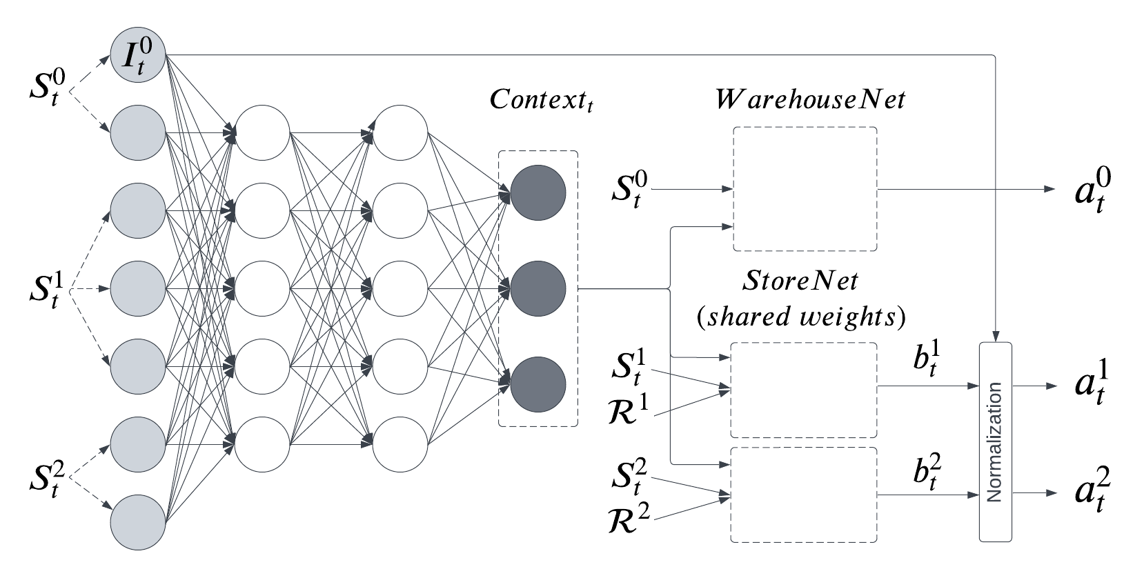
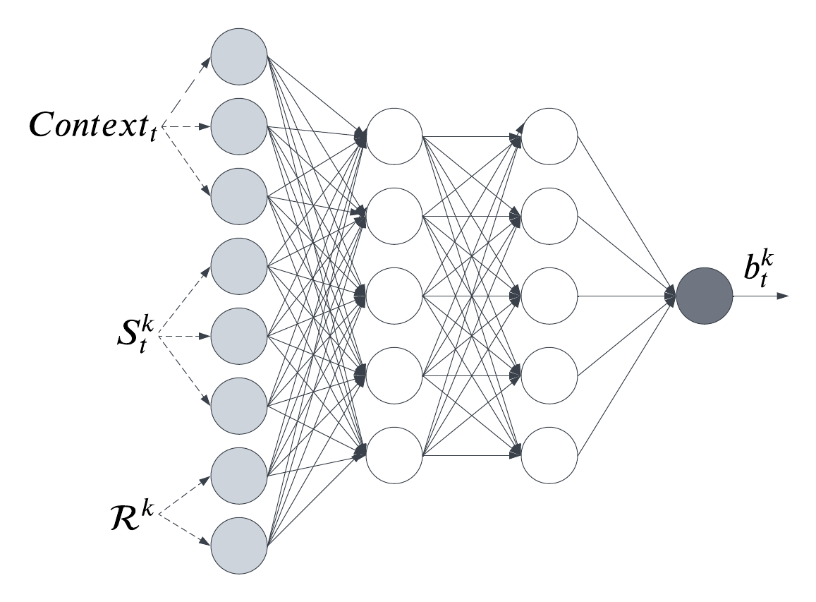
Instead, we introduce the Symmetry-aware NN architecture, which mimics the physical structure of the inventory network, and leverages weak coupling between locations and the symmetry among stores. Specifically, since the different individual actions (the store orders and the warehouse order) are only weakly related to each other, our NN architecture incorporates a separate Warehouse Net and a Store Net, with a copy of the latter (with identical weights) for each store. Instead of the full system state being provided as an input to each of these Nets, a Context Net compresses the overall state, and its output – termed the current context – is provided as input to the Warehouse and Store Nets, along with relevant local information. Each of the Nets is a standard MLP. The general scheme is shown in Figure 3 in the appendix. The Warehouse Net is fed the warehouse’s state and the context, and directly outputs an order amount. The copy of the Store Net for store is fed the store’s local state , local primitives (e.g., cost parameters, lead time, sample mean and variance of demand), and the context, and outputs a tentative allocation . Finally, tentative allocations are normalized before outputting each store’s allocation. The Store Net is depicted in Figure 4. Our NN architecture is found to perform well under a variety of problem settings and sizes, as described in Section 4.
3.1 Why should a symmetry-aware policy work well?
In this section, we build understanding for why symmetry-aware policies lead to good performance in inventory control problems by establishing a formal guarantee for an example setting, described in Example 1. The guarantee formalizes the intuition that each store (and the warehouse) does not need to know the full state of the system to choose a good ordering action; instead, it suffices to inform it of its local state together with an overall sense of inventory scarcity in the network.
Definition 1.
Let be a mapping from state to a dimensional “context” vector for some , and be mappings for every location . We say is a symmetry-aware policy with -dimensional context if it is of the form
We call the context mapping and the context-dependent local policy of location .
As described above, our implementation exploits symmetries across stores by using weight sharing. Definition 1 is meant to isolate one feature of the problem—the use of a Context Net to summarize the overall state—and hence allows for the possibility each Store Net is heterogeneous.
Example 1.
Consider stores and one warehouse, with backlogged demand (3). The underage and holding costs of each store satisfy satisfy and for some . Demand is of the form , where is drawn independently across stores and time (with for some ), and is drawn independently across time; it takes a high value with probability and a low value otherwise. The warehouse lead time is and store lead time is . The system starts with zero inventory. We make two extra assumptions. First, for every , which ensures that, if store starts with an inventory no larger than , the remaining inventory after demand is realized is below . Second, , which ensures that it is worth acquiring an incremental unit of inventory at the warehouse if that is sure to prevent a lost sale in a period of high demand.
We comment briefly on the structure of this example setting. Here, due to the aggregate demand being either “high” or “low” in each period, and the lead time of the warehouse being 1 period, in each period there is either a scarcity or an abundance of inventory in the network, due to the aggregate demand having been “high” or “low”, respectively, in the previous period. As a result, both the warehouse and the stores do need some information about the inventory state to place an appropriate order. We believe it is possible to prove making local orders without knowledge of the global state necessarily leads to an percentage increase in the cost incurred under certain problem primitives.
We establish the following guarantee of asymptotic optimality in per-period costs of a symmetry-aware policy with 1-dimensional context, as the number of stores grows. The proof is given in Appendix D. It constructs an asymptotically optimal policy in which the warehouse follows an echelon-stock policy and each store a base-stock policy (see Appendix B), with the current base-stock level depending only on an estimate of whether the previous system-wide demand was high or low; This is signaled by a context mapping that maps to the sum of its components .
Theorem 1.
In Example 1, let be the expected total cost incurred by policy from the initial state. There exists such that the following occurs. There exists a stationary symmetry-aware policy with -dimensional context which satisfies .
4 Numerical experiments
We subjected our methodology to two types of experimental evaluations. First, Section 4.1 reports results on four settings in which either the optimal average per-period cost or a sufficiently “tight” lower bound for it can be computed. Our method consistently exploits each problem’s hidden structure to obtain (essentially) optimal average cost. Subsections 4.1.1 and 4.1.2 reveal that HDPO and the Symmetry-aware NN architecture drive these outstanding results. Second, Section 4.2 shows that our approach vastly outperforms problem-dependent heuristics in settings where a good lower bound on the optimal cost is not available.
Overview of implementation details. Precise experiment details are presented in Appendix C. We developed a differentiable simulator using PyTorch and executed all experiments on an NVIDIA A40 with 48GB of memory. All trainable benchmark policies were also optimized using our differentiable simulator; we restart their training multiple times and report the best results attained. Unless otherwise specified, we use a only a single training run for our policy. To mimic an infinite horizon stationary setting, we train the parameters of a stationary policy to minimize cost accrued over episodes of long duration. We typically drew initial states from a uniform distribution, which seemed to expedite convergence, but in a few cases we used a fixed initial state. To avoid reporting “transient” effects, the metrics we report exclude a given number of early periods. All reported metrics are based on a clean test set, which was not used for training or hyperparameter tuning, unless otherwise specified.
All layers except one used Tanh as the activation function, which enabled faster and more stable learning than ReLU. We discuss how we tuned the number of layers and neurons per layer and report all hyperparameter specifications in the appendices. In general, some ad-hoc tuning was done when treating substantially different inventory network structures.444The serial system in Table 1 is very different from the one store, no warehouse problem. We employed only one “trick”, which we found to be crucial. We fix a very crude upper bound on the amount of inventory any location should order555E.g., if lead time is 5, and the 99.9th percentile of demand within a period is 100, then a store should not hold more than 500 units of inventory. and call this the maximum-allowable order. Then, we obtain tentative allocations/orders (see Sec 3) by applying a Sigmoid activation function and multiplying by the max-allowable order.
4.1 Our method recovers near-optimal policies
Table 1 summarizes the performance (average cost per period) of the Vanilla NN for four settings where we can compare the performance to the optimal cost or a provable lower bound, across multiple instances. For each setting, we maintain the same hyperparameter values across instances and report the cost of a single run over each instance. Our results demonstrate that the Vanilla NN can consistently and reliably recover near-optimal policies for medium-sized problems, even when using raw state inputs. In the last setting, as the number of stores grows past , the performance of the Vanilla NN degrades (extensive hyperparameter tuning fails to resolve the issue, see Appendix C.6), motivating our Symmetry-aware NN described in Section 3. The Symmetry-aware NN performs well even as the number of stores grows (see Section 4.1.2). For instances with over dimensions in the state space, we obtained optimality gaps smaller than %. Our main findings can be summarized as follows: i) Vanilla NNs can recover near-optimal policies in moderate-sized problems; ii) training with HDPO allows for fast and stable learning with a broad range of hyperparameters; and iii) Symmetry-aware NNs allow to efficiently recover near-optimal policies, regardless of the number of stores being small, moderate, or large. We delve deeper into two settings to illustrate these findings.
|
|
|
Benchmark |
|
|
|
||||||||||||||||
|---|---|---|---|---|---|---|---|---|---|---|---|---|---|---|---|---|---|---|---|---|---|---|
|
Backlogged | 1 to 20 |
|
24 | 0.09 | 0.26 | ||||||||||||||||
|
Lost | 1 to 4 |
|
16 | <0.25 | <0.25 | ||||||||||||||||
| Serial | Backlogged | 10 to 13 |
|
16 | 0.39 | 1.57 | ||||||||||||||||
|
Backlogged | 9 to 63 |
|
36 | <=0.20 | <= 0.79 |
4.1.1 On the benefits of hindsight differentiable policy optimization
Gijsbrechts et al. [13] tested their A3C approach on 6 out of 16 instances from the classic inventory control paper Zipkin [38], which considers a single store facing a stationary Poisson demand, under lost demand and discrete allocation (second row in Table 1). We replicated the test-bed of 16 instances from Zipkin [38] by setting , , and . We trained our model as if actions were continuous, and rounded allocations to the nearest integer at test-time. To test the robustness to hyperparameter choices, we considered architectures with two and three hidden layers, learning rates of , and , and batch sizes of and , running them once on all instances. Appendix C.4 presents detailed results in Tables 4 and 5, and shows very stable and rapid learning across the entire range of hyperparameter values, for all 16 instances. Our method achieved the minimum detectable optimality gap666Costs in [38] are reported with decimals. The smallest optimal average cost is around , and so an optimality gap of smaller than cannot be detected. of on of the runs, with the optimality gap always being below . In contrast, Gijsbrechts et al. [13] reported that their A3C algorithm was highly sensitive to hyperparameters and required extensive tuning. Their algorithm achieved optimality gaps between and for the best run among around hyperparameter combinations.
4.1.2 On the benefits of Symmetry-aware NNs
We consider the setting introduced in Federgruen and Zipkin [8], where a warehouse operates as a transshipment center (i.e., cannot hold inventory) and there are multiple stores, under a backlogged demand assumption (fourth row in Table 1). The demand is i.i.d. across time but may be correlated across stores. To apply a known analytical lower bound on the optimum, we assume all stores have the same per-unit costs and lead time. We created instances by considering , , and three levels of pairwise correlation in demands (the store-level marginal demand distributions are assumed to be normal, with distinct means and variances across stores). We present the complete results in Table 8 in Appendix B.4. The Vanilla NN achieved an average gap under , and on every instance, including those with a -dimensional state space, the gap was under . Moreover, it was able to achieve a dev-set gap below % in less than minutes on average.
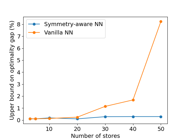
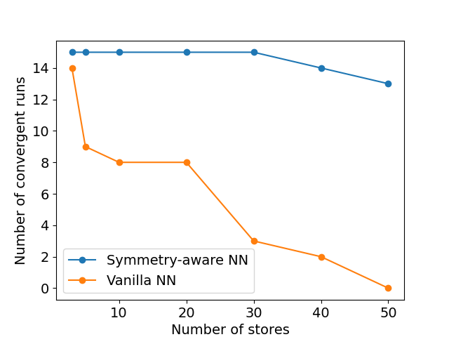
We conducted further testing to evaluate the performance of the Symmetry-aware NN compared to the Vanilla NN as the number of stores increases. We fixed , , and pairwise correlation to , and varied from to . We performed extensive hyperparameter tuning for both models, especially for large . After arriving at the optimal configuration for each setting, we conducted five runs of the model for each of three different learning rates around the best-performing one to assess the stability and robustness of each method. Figures 1(a) and 1(b) show the smallest optimality gap across runs and the number of runs that converged to a solution with a gap smaller than for each instance. The Vanilla NN performs well and consistently up to stores, but its performance begins to significantly degrade beyond that point. On the other hand, the Symmetry-aware NN consistently performs well. For the stores scenario, which involves a -dimensional state, it achieved a gap of less than (the stores instance is excluded from the figures, which stop at 50 stores).
best-performing run.
solution with optimality gap smaller than .
4.2 Outperforming problem-dependent heuristics
It is possible for our methodology to vastly outperform existing heuristics in complex settings without a simple solution structure. We illustrate this through an example. It considers a scenario with only one store and no warehouse, incorporating a lost demand assumption and time-correlated demand, which is a prevalent feature in practical situations. Our test-bed consisted of eight instances in which demand was modeled as , where is an AR() process (i.e., an autoregressive process of order ) and is a fixed number. Two heuristics were evaluated in our comparison. The first, called the Capped Base Stock policy [37], is cognizant of the inventory pipeline and has demonstrated excellent performance in settings with lost demand, but without temporal correlation. The second is a quantile policy, which first leverages the historical demand information to calculate the current posterior distribution of “inventory depletion” in the next period as if demand was backlogged, and then optimizes a specific quantile of the distribution to determine the order quantity. The performance of the two heuristics varied widely for different instances, with each incurring at least larger cost than our approach in at least one instance. Detailed results can be found in Table 11 in Appendix C.7.
Acknowledgement
After beginning our numerical experiments, we learned of the work of Madeka et al. [24]. We thank them for their open and collaborative outlook, and their very helpful feedback.
Appendix A Outline of the appendix
We divide the Appendix into large sections. In Appendix B, we provide a detailed description of each of the problem types addressed. For problems discussed in Section 4.1, we show how we obtained the optimal cost or lower bound, and for the ones in Section 4.2, we detail the best-performing heuristics we used as benchmarks. In Appendix C, we provide details on the implementation of our models, the process of hyperparameter tuning and numerical results. Finally, in Appendix D we provide a full proof of Theorem 1.
Appendix B Description of problem settings and benchmarks
We begin by providing an overview of settings we will cover and their respective optimal policy structures or well-performing heuristics.
B.1 One store, no warehouse. Backlogged demand assumption.
This setting consists of a single store with known per-unit underage and holding costs and a deterministic lead time . In each period, the store faces an independent, identically distributed (i.i.d.) demand with distribution , and has access to a supplier with infinite inventory. Under linear costs, a base-stock policy is optimal [31]. We define the store’s inventory position at time as
| (7) |
The optimal policy then takes the form
| (8) |
for some constant base-stock level . Furthermore, as there are no procurement costs, the optimal base stock level can be calculated as
| (9) |
where is the distribution of the cumulative demand in periods.
B.2 One store, no warehouse. Lost demand assumption.
This setting is identical to that in Appendix B.1, except that demand is assumed to be lost if not satisfied immediately (e.g., consumers may buy from the competition if a product is not available.). This assumption may better represent reality especially in brick and mortar retail, as depending on product category, only of customers are willing to delay their purchase when not finding a specific item at a store [6].
A base-stock policy is no longer optimal in this setting under a lead time of at least of period, and its performance deteriorates as the lead time grows. Furthermore, the optimal policy does not appear to have a simple structure, and may depend on the complete inventory pipeline. Solving this problem exactly is computationally intractable even for medium-sized instances. Therefore, numerous heuristics have been proposed. Arguably the best-performing heuristic for this setting considers the family of Capped Base Stock (CBS) policies [37], which achieve an average optimality gap of in the 32-instance test-bed proposed in [38]. A CBS policy is defined by a base stock level and an order cap , as per
| (10) |
B.3 Serial network structure. Backlogged demand assumption.
In this setting, the system consists of echelons, each comprising a single location. Locations are sequentially numbered from to , starting from the upstream and progressing towards the downstream. Demand arises solely at the most downstream location (location ), and any unfilled demand is backlogged. Inventory costs, denoted as , are incurred at each location, and there is an underage cost of per unit at the downstream location. Each location has a positive lead time denoted as . It is assumed that demand is i.i.d. over time.
The sequence of events is as follows: A central planner observes the state at time and jointly determines the order that the first location places with an external supplier with unlimited inventory and, for , specifies the quantity to transfer from location to location , ensuring that it does not exceed the current inventory level at location (i.e., , ).
We define the echelon inventory position of location at time as
| (11) |
with the inventory position of store as defined in (7). That is, it represents the sum over all inventory positions of downstream locations and its own. As shown by Clark and Scarf [5], the optimal policy takes the form
| (12) | ||||
for some echelon base-stock levels . We note that we will use the terms echelon base-stock levels and echelon-stock levels interchangeably. We refer to (12) as an Echelon-stock policy.
B.4 Many stores, one warehouse. Backlogged demand assumption.
We consider the setting introduced in Federgruen and Zipkin [8], where a warehouse operates as a transshipment center (i.e., cannot hold inventory) and there are multiple stores, under a backlogged demand assumption. The demand is i.i.d. across time but may be correlated across stores. The costs incurred solely consider holding and underage costs at the stores.
Federgruen and Zipkin [8] provide a clever way to obtain a lower bound when demand at the stores follows a jointly normal demand, and store costs and lead times are identical. To leverage their results, we assume that all stores have the same underage costs denoted as and lead time denoted as , while the warehouse has a lead time of . For each store , we consider a marginal demand that follows a normal distribution with mean and standard deviation . Furthermore, we represent the covariance matrix as , where denotes the covariance between the demands of stores and .
The echelon inventory position at the warehouse takes the form
| (13) |
where denotes the inventory position of location as defined in (7). That is, represents the sum of the inventory position across stores plus its own. The authors consider a relaxation of the problem by allowing inventory to flow from stores to the warehouse and to other stores. The authors demonstrate that it is possible to reformulate the problem using the echelon inventory position as the state variable. They establish that the Bellman Equation in this relaxed setting can be expressed as a single-location inventory problem with convex costs. Consequently, they deduce that an optimal policy for the warehouse, in the relaxed problem, is an echelon-stock policy. Finally, as we do not consider purchase costs, the optimal base-stock level can be calculated analytically via the newsvendor-type formula
| (14) |
where is a normal distribution with mean and standard deviation given by
Now, let be a standardized version of . The lower bound on costs per-period is finally given by
with and the Cumulative Distribution Function and Probability Density Function, respectively, of a standard Normal distribution.
We note that the previous quantity is not normalized by the number of stores.
B.5 One store, no warehouse. Backlogged demand assumption and time-correlated demand.
This setting is identical to that in Appendix B.2, except that demand is assumed to be correlated across time. Specifically, demand at time takes the form , where is an AR() process (i.e., an autoregressive process of order ) and is a fixed number. Thus, for , takes the form
for some parameter vector , and with a white noise that distributes according to a standard Normal distribution.
We tested heuristics on this setting, as described in Section 4.2, which we now describe.
Capped Base Stock Policy
A full description is given in Appendix B.2. Its structure follows (10). This heuristic is cognizant of the inventory pipeline and has demonstrated excellent performance in settings with lost demand, but without temporal correlation.
Quantile policy
This policy leverages the historical demand information to calculate the current posterior distribution of “inventory depletion” in the next period as if demand was backlogged, and then optimizes a specific quantile of the distribution to determine the order quantity.
On period , conditional on , the random variable is a jointly normal random variable. We therefore have that the cumulative demand over the next periods conditional on follows a normal distribution , with mean and variance that depend on . The quantile policy then takes the form
with a trainable parameter.
Appendix C Implementation details and numerical experiments
This section offers a comprehensive account of our implementation and numerical experiments. In Appendix C.1, we define some terminology and we outline the architectures of our Neural Networks, as well as the procedures employed for training and hyperparameter tuning. Appendix C.2 specifies the best-performing hyperparameter setting and the initialization procedure for each problem setting. In the remaining subsections, we present all information required to replicate our experiments accurately. We provide detailed descriptions of the experimental setup, comprehensive results, and a concise analysis of the outcomes.
C.1 Implementation details
Terminology and reporting conventions
We briefly introduce the terminology required to follow our experiments and setup
-
•
Hyperparameter: A parameter that is set before the learning process begins and affects the model’s behavior or performance.
-
•
NN architecture: Overall topology and organization of the network, which determines how information flows through the network and how computations are performed.
-
•
NN module: A distinct component or sub-network within a larger NN architecture, which performs a specialized computation or processing task. The Symmetry-aware NN has three modules (with one copy of the Store Net module for each store), while the Vanilla NN has only one module.
-
•
Epoch: A complete pass through the entire training dataset during the training process.
-
•
Batch: A subset of the training dataset used for updating model parameters.
-
•
Batch size: The number of samples included in each batch.
-
•
Gradient step: A step taken to update the model’s parameters based on the gradient computed over one batch.
-
•
Learning rate: A hyperparameter that determines the step size of the gradient step.
-
•
Hidden layer: A layer in a neural network that sits between the input and output layers and performs intermediate computations.
-
•
Unit/neurons: Fundamental unit of a neural network that receives input, performs a computation, and produces an output.
-
•
Configuration: A specific combination of a hyperparameter setting and a state initialization procedure.
We outline the reporting convention that will be followed throughout this section.
-
•
Units per layer: The count of units or neurons present in each hidden layer of a NN module. We present this information as a tuple. For the Symmetry-aware, we define the order (Context Net, Warehouse Net, Store Net) for reporting, so, for example, the second component represents the number of units in all the hidden layers of the Warehouse Net. For the Vanilla NN, we report a single number indicating the number of units in each hidden layer.
-
•
Loss: The average cost incurred per period and per store in a given dataset. Calculated by dividing the total cost accumulated across the periods considered by the number of stores and periods considered.
-
•
Gap: The percentage difference between the cost incurred by a policy and a predefined benchmark cost. The benchmark cost can take the form of the optimal cost, a lower bound on costs, or the cost incurred by a heuristic approach.
Neural Network Architectures
We implemented all our Neural Networks using one or more fully connected Multilayer Perceptrons (MLP). Figure 2 shows a diagram of our Vanilla NN, while Figures 3 and 4 depict the Symmetry-aware NN and the Store Net, respectively.
The Vanilla NN takes the raw state as input and outputs an allocation for the warehouse and tentative allocations for each store.
The Symmetry-aware NN incorporates a separate Warehouse Net and a Store Net, with a copy of the latter (with identical weights) for each store. Instead of the full system state being provided as an input to each of these Nets, a Context Net compresses the overall state, and its output – termed the current context – is provided as input to the Warehouse and Store Nets, along with relevant local information. The Warehouse Net is fed the warehouse’s state and the context, and directly outputs an order amount. The copy of the Store Net for store is fed the store’s local state , local primitives (e.g., cost parameters, lead time, sample mean and variance of demand), and the context, and outputs a tentative allocation .

For both NNs, all layers except the output layers which generate allocation quantities used Tanh as the activation function, which enabled faster and more stable learning than ReLU. In all scenarios except for the serial network structure, we interpret the outputs of the Store Net and the last outputs of the Vanilla NN as tentative store allocations, denoted as . To obtain the final allocations, we normalize these tentative allocations using the function . Store allocations are finally obtained as . We employed only one “trick”, which we found to be crucial. We fixed a very crude upper bound on the amount of inventory any location should order and call this the max-allowable order. An example of such a crude bound is as follows: if lead time is 5, and the 99.9th percentile of demand within a period is 100, then a store should not hold more than 500 units of inventory. It should be emphasized that in our implementation the maximum-allowable order remains constant across stores in scenarios involving multiple heterogeneous stores. We obtain tentative allocations/orders (see Sec 3) by applying a Sigmoid activation function and multiplying by the max-allowable order.
For the serial network structure, we experimented with the Vanilla NN using a similar architecture. In this setup, for , the -th output of the NN was considered as a tentative allocation for ordering from the parent location in the supply chain. These tentative allocations were capped at the inventory available at the parent location. However, we encountered situations where this policy became trapped in what we believe were suboptimal local optima. To address this issue, we explored an alternative architecture. In this approach, the -th output of the NN was interpreted as the fraction of the preceding location’s inventory-on-hand to order. Consequently, if represents the -th output and denotes the inventory on-hand at the preceding location, the final allocations were calculated as . This modified approach consistently yielded near-optimal performance in our experiments. For the first location, we employed the previously described “trick”, in which we apply a Sigmoid activation function and multiply by a crude upper bound.
Initialization
We used two different procedures to initialize the on-hand inventories and vectors of outstanding orders for stores.
-
•
Uniform: letting be the sample mean demand for store , we initialized and every entry in by sampling independently (across and , and across ) from .
-
•
Set to : we simply set and every entry in to .
For the warehouse’s inventory on-hand and vector of outstanding orders , we set each entry to . Finally, for time-correlated demand of the form as described in Appendix B.5, we set the previous terms of the AR sequence to , this is, .
Training and reporting
We utilized three separate datasets: a train set for model training, a dev set for hyperparameter tuning and model selection, and a test set for evaluating the models’ performance over a longer time horizon and estimating per-period costs. To mimic an infinite horizon stationary setting, we train the parameters of a stationary policy to minimize cost accrued over episodes of long duration. To avoid reporting “transient” effects, the metrics we report exclude a given number of early periods. All reported metrics are based on a clean test set, which was not used for training or hyperparameter tuning, unless otherwise specified. The trainable benchmark policies were trained using our differentiable simulator, and we report the best results obtained from multiple training runs.
Throughout our experiments, we fixed the number of periods to 50 and excluded the first 30 periods when calculating costs for the training and development sets. For the test set, we extended the number of periods to 500 and excluded the initial 300 periods.
To determine the termination point for training, we utilize a straightforward criterion of specifying a fixed number of epochs. Training is concluded once the specified number of epochs has been reached. It is important to note that the number of epochs can vary significantly across different settings. We set the number of epochs based on prior knowledge of the approximate number required to achieve near-optimal solutions.
Hyperparameter tuning
We found that our method exhibited robustness to the choice of hyperparameters, requiring minimal tuning effort in most cases. Initially, we conducted experiments to explore various combinations of hyperparameters such as learning rates, batch sizes, number of hidden layers, and number of neurons per layer. Through this process, we identified a set of hyperparameter combinations that yielded satisfactory performance. However, when dealing with substantially different inventory network structures, such as the serial one, we performed some ad-hoc tuning by searching for hyperparameter values on a grid.
The only scenario that required substantial hyperparameter tuning was for the experiments comparing the performance of the Vanilla NN and the Symmetry-aware NN for an increasing number of stores, as described in Section 4.1.2. We describe our hyperparameter tuning process in more detail in Appendix C.6.
Technical implementation specifications
We developed a differentiable simulator using PyTorch and conducted all experiments on an NVIDIA A40 GPU with 48GB of memory. To expedite the training process, we implemented an efficient parallel computation scheme. For a given mini-batch of sample paths, we simultaneously executed the forward and backward passes across all sample paths. To achieve this, we utilized an initial mini-batch “state” matrix denoted as . This matrix was obtained by stacking the initial states for each sample path . At each time period, we input the matrix into the neural network, enabling us to obtain the outputs for every sample path in a highly parallelizable manner. Subsequently, we computed the costs and updated the mini-batch state matrix through efficient matrix computations. This approach allowed PyTorch to efficiently estimate the gradients during the backward pass.
C.2 Hyperparameter settings and state initialization
Table 2 presents the best-performing configuration for each setting for the Vanilla NN. The reported results for fixed hyperparameters in Appendices C.3 through C.7 are based on these configurations. However, it is worth noting that a wide range of hyperparameters generally yield satisfactory performance, except for very large-scale problems where hyperparameters needed to be tuned on a per-instance basis.
| Setting description |
|
|
|
|
|
||||||||||
|---|---|---|---|---|---|---|---|---|---|---|---|---|---|---|---|
|
2 | 32 | 0.0001 | 8192 | Uniform | ||||||||||
|
2 | 32 | 0.0001 | 8192 | Uniform | ||||||||||
|
2 | 32 | 0.001 | 8192 | Set to 0 | ||||||||||
|
3 | 32 | 0.0001 | 1024 | Uniform | ||||||||||
|
2 | 64 | 0.0001 | 512 | Uniform |
C.3 One store, no warehouse. Backlogged demand assumption.
We consider a Normal demand with mean and standard deviation , and truncate it at from below. We created instances by setting , and . We compare our model with the optimal base-stock policy computed according to (8) and (9) in Appendix B.2.
Figures 5(a) and 5(b), respectively, show the optimality gap and time to reach of optimality gap. Our approach achieves an average gap of across instances and takes less than minutes, on average, to obtain a gap. Further, gaps are consistently below across instances, even for long lead times of up-to periods. We report additional performance indicators in Table 3.
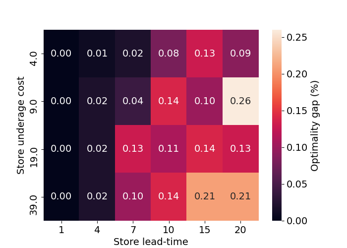
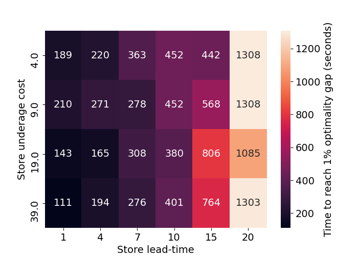
| Store leadtime | Store underage cost | Train loss | Dev loss | Test loss | Train gap (%) | Dev gap (%) | Test gap (%) | Epochs to 1% dev gap |
|---|---|---|---|---|---|---|---|---|
| 1 | 4 | 3.17 | 3.17 | 3.17 | 0.01 | 0.01 | 0.00 | 181 |
| 1 | 9 | 3.97 | 3.98 | 3.97 | 0.00 | 0.00 | 0.00 | 193 |
| 1 | 19 | 4.67 | 4.67 | 4.67 | 0.01 | -0.01 | 0.00 | 195 |
| 1 | 39 | 5.29 | 5.30 | 5.29 | 0.01 | 0.00 | 0.00 | 154 |
| 4 | 4 | 5.01 | 5.02 | 5.00 | 0.01 | 0.00 | 0.01 | 186 |
| 4 | 9 | 6.28 | 6.29 | 6.28 | 0.01 | 0.04 | 0.02 | 233 |
| 4 | 19 | 7.38 | 7.37 | 7.38 | 0.02 | 0.02 | 0.02 | 179 |
| 4 | 39 | 8.36 | 8.40 | 8.35 | 0.01 | 0.01 | 0.02 | 210 |
| 7 | 4 | 6.33 | 6.34 | 6.34 | 0.02 | 0.01 | 0.02 | 274 |
| 7 | 9 | 7.94 | 7.96 | 7.94 | 0.03 | 0.03 | 0.04 | 210 |
| 7 | 19 | 9.37 | 9.34 | 9.35 | 0.14 | 0.11 | 0.13 | 259 |
| 7 | 39 | 10.58 | 10.60 | 10.57 | 0.10 | 0.09 | 0.10 | 226 |
| 10 | 4 | 7.45 | 7.37 | 7.44 | 0.09 | 0.07 | 0.08 | 311 |
| 10 | 9 | 9.31 | 9.30 | 9.33 | 0.12 | 0.17 | 0.14 | 311 |
| 10 | 19 | 10.95 | 11.10 | 10.96 | 0.10 | 0.12 | 0.11 | 337 |
| 10 | 39 | 12.44 | 12.36 | 12.43 | 0.14 | 0.14 | 0.14 | 357 |
| 15 | 4 | 8.98 | 8.91 | 8.94 | 0.09 | 0.15 | 0.13 | 346 |
| 15 | 9 | 11.22 | 11.26 | 11.24 | 0.08 | 0.15 | 0.10 | 448 |
| 15 | 19 | 13.22 | 13.17 | 13.21 | 0.10 | 0.15 | 0.14 | 597 |
| 15 | 39 | 14.95 | 14.88 | 14.99 | 0.19 | 0.27 | 0.21 | 576 |
| 20 | 4 | 10.26 | 10.31 | 10.25 | 0.17 | 0.15 | 0.09 | 800 |
| 20 | 9 | 12.92 | 12.93 | 12.92 | 0.28 | 0.42 | 0.26 | 800 |
| 20 | 19 | 15.12 | 15.15 | 15.15 | 0.26 | 0.29 | 0.13 | 707 |
| 20 | 39 | 17.17 | 17.26 | 17.17 | 0.05 | 0.28 | 0.21 | 864 |
C.4 One store, no warehouse. Lost demand assumption.
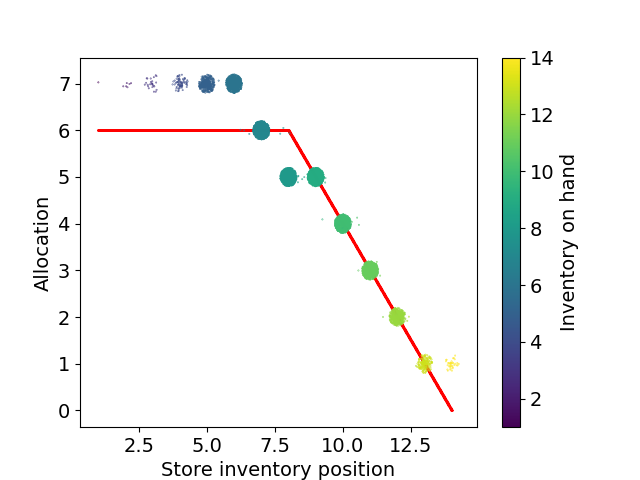
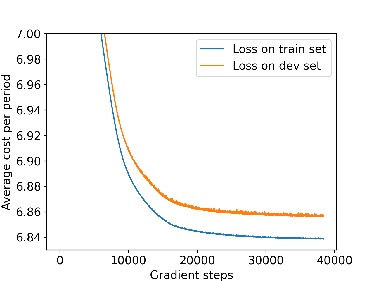
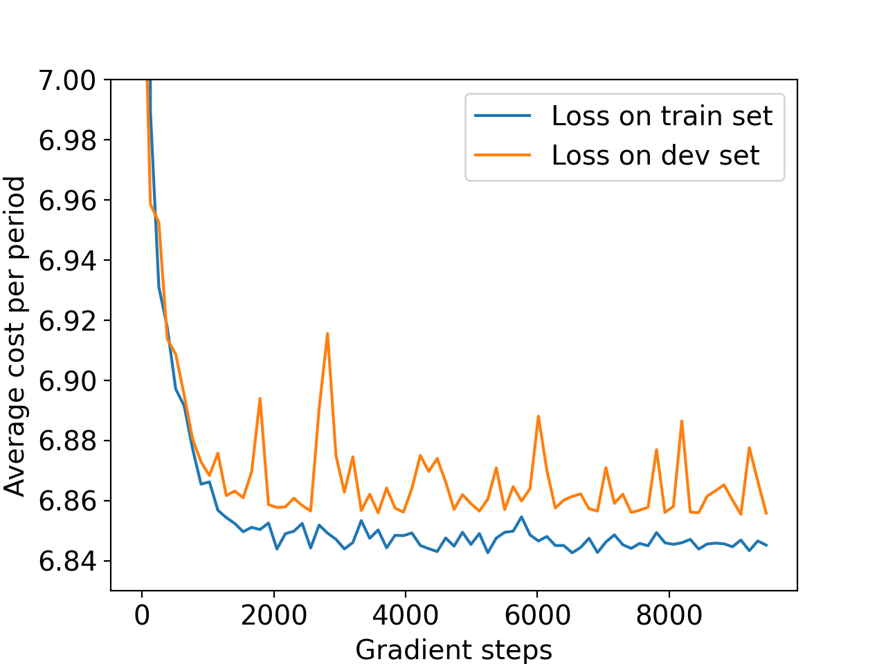
The details of the test-bed considered for this setting can be found in Section 4.1.1. We report the performance under the best hyperparameter setting and the average performance for every hyperparameter setting separately in Tables 4 and 5, respectively. We also report the performance of the optimal CBS policy (as given in [37]) in Table 6. In Figure 6 we plot the inventory position and allocation under the Vanilla NN policy for settings and compare it to the allocation under the optimal CBS policy (red line). We randomly jitter points for visibility, and color points according the current inventory on-hand. We observe that the structure of the policy learned by our Vanilla NN somewhat resembles a CBS policy, but our learned policy is able to use additional information in the state space to achieve lower costs. For a fixed inventory position (see (7)), the NN tends to order less for lower inventory on hand, as a stock-out is more likely under such a scenario in which case less inventory will actually be depleted. Finally, Figure 7 shows the learning curves on one instance for two “extreme” choices of hyperparameters, revealing stable learning and rapid convergence to near-optimal solutions across all hyperparameter settings.
| Store lead time | Store underage cost | Test loss | Test gap (%) | Gradient steps to 1% dev gap | Time to 1% dev gap (s) |
| 1 | 4 | 4.04 | <0.25 | 2912 | 138 |
| 1 | 9 | 5.43 | <0.25 | 4848 | 283 |
| 1 | 19 | 6.67 | <0.25 | 4704 | 225 |
| 1 | 39 | 7.85 | <0.25 | 2768 | 139 |
| 2 | 4 | 4.40 | <0.25 | 3792 | 192 |
| 2 | 9 | 6.09 | <0.25 | 5328 | 284 |
| 2 | 19 | 7.67 | <0.25 | 17008 | 871 |
| 2 | 39 | 9.09 | <0.25 | 2112 | 112 |
| 3 | 4 | 4.60 | <0.25 | 9536 | 504 |
| 3 | 9 | 6.53 | <0.25 | 4608 | 263 |
| 3 | 19 | 8.37 | <0.25 | 5008 | 268 |
| 3 | 39 | 10.03 | <0.25 | 6960 | 389 |
| 4 | 4 | 4.73 | <0.25 | 12032 | 668 |
| 4 | 9 | 6.84 | <0.25 | 4288 | 252 |
| 4 | 19 | 8.89 | <0.25 | 3328 | 185 |
| 4 | 39 | 10.80 | <0.25 | 4192 | 230 |
|
|
|
|
|
|
||||||||||||||
|---|---|---|---|---|---|---|---|---|---|---|---|---|---|---|---|---|---|---|---|
| 2 | 1024 | 0.0001 | 15 | 15232 | 746 | ||||||||||||||
| 2 | 1024 | 0.0010 | 16 | 5392 | 248 | ||||||||||||||
| 2 | 1024 | 0.0100 | 14 | 3936 | 182 | ||||||||||||||
| 2 | 8192 | 0.0001 | 16 | 11596 | 649 | ||||||||||||||
| 2 | 8192 | 0.0010 | 16 | 4653 | 253 | ||||||||||||||
| 2 | 8192 | 0.0100 | 16 | 2450 | 132 | ||||||||||||||
| 3 | 1024 | 0.0001 | 16 | 8984 | 510 | ||||||||||||||
| 3 | 1024 | 0.0010 | 16 | 6688 | 371 | ||||||||||||||
| 3 | 1024 | 0.0100 | 13 | 3352 | 176 | ||||||||||||||
| 3 | 8192 | 0.0001 | 16 | 10492 | 703 | ||||||||||||||
| 3 | 8192 | 0.0010 | 16 | 6040 | 374 | ||||||||||||||
| 3 | 8192 | 0.0100 | 16 | 2326 | 180 |
| Store leadtime | Store underage cost | Test loss | Test gap (%) |
| 1 | 4 | 4.06 | 0.50 |
| 1 | 9 | 5.48 | 0.74 |
| 1 | 19 | 6.69 | 0.15 |
| 1 | 39 | 7.85 | 0.13 |
| 2 | 4 | 4.41 | 0.23 |
| 2 | 9 | 6.11 | 0.33 |
| 2 | 19 | 7.71 | 0.65 |
| 2 | 39 | 9.13 | 0.22 |
| 3 | 4 | 4.63 | 0.65 |
| 3 | 9 | 6.61 | 1.23 |
| 3 | 19 | 8.39 | 0.36 |
| 3 | 39 | 10.07 | 0.30 |
| 4 | 4 | 4.80 | 1.48 |
| 4 | 9 | 6.91 | 1.02 |
| 4 | 19 | 8.95 | 0.67 |
| 4 | 39 | 10.90 | 1.02 |

and batch size of .
and batch size of .
C.5 Serial network structure. Backlogged demand assumption.
We analyzed a serial network structure with echelons. We considered Normal demand with mean and standard deviation , and truncated it at from below. We fixed holding costs as , , and . The lead times for the first echelons are fixed as , and . We created instances by setting and .
Within this scenario, there exists an optimal echelon-stock policy ((11) in Appendix B.3). We employ our differentiable simulator to search for the best-performing base-stock levels through multiple runs. We then compare our NNs with the best-performing echelon-stock policy obtained, which we take as the optimal cost.
Table 7 describes the performance of the Vanilla NN for each instance of the serial network structure described in Appendix B.3, for the configuration in Table 2. The Vanilla NN achieved an average optimality gap of , and needed around gradient steps, on average, to achieve a gap smaller than in the dev set.
| Store lead time | Store underage cost | Train loss | Dev loss | Test loss | Train gap (%) | Dev gap (%) | Test gap (%) | Gradient steps to 1% dev gap |
|---|---|---|---|---|---|---|---|---|
| 1 | 4 | 6.91 | 6.89 | 6.91 | 0.00 | 0.10 | 0.10 | 5088 |
| 1 | 9 | 8.37 | 8.40 | 8.38 | 0.10 | 0.12 | 0.12 | 3472 |
| 1 | 19 | 9.62 | 9.61 | 9.63 | 0.04 | 0.35 | 0.24 | 3456 |
| 1 | 39 | 10.71 | 10.69 | 10.77 | 0.17 | 0.28 | 0.34 | 5408 |
| 2 | 4 | 7.62 | 7.67 | 7.64 | 0.23 | 0.32 | 0.33 | 5456 |
| 2 | 9 | 9.26 | 9.34 | 9.29 | 0.12 | 0.26 | 0.21 | 3904 |
| 2 | 19 | 10.69 | 10.72 | 10.72 | 0.08 | 0.31 | 0.30 | 4416 |
| 2 | 39 | 11.97 | 11.92 | 11.94 | 0.24 | 0.44 | 0.42 | 6240 |
| 3 | 4 | 8.23 | 8.26 | 8.25 | 0.14 | 0.34 | 0.32 | 5856 |
| 3 | 9 | 10.07 | 10.09 | 10.07 | 0.20 | 0.40 | 0.41 | 4912 |
| 3 | 19 | 11.64 | 11.73 | 11.65 | 0.30 | 0.51 | 0.47 | 5248 |
| 3 | 39 | 12.96 | 13.03 | 13.02 | 0.23 | 0.45 | 0.39 | 5328 |
| 4 | 4 | 8.78 | 8.83 | 8.78 | 0.22 | 0.36 | 0.38 | 5488 |
| 4 | 9 | 10.78 | 10.77 | 10.77 | 0.19 | 0.35 | 0.33 | 5200 |
| 4 | 19 | 12.47 | 12.44 | 12.48 | 0.25 | 0.21 | 0.33 | 4048 |
| 4 | 39 | 13.98 | 14.08 | 14.10 | 0.49 | 0.87 | 1.57 | 6368 |
C.6 Many stores, one warehouse. Backlogged demand assumption.
To supplement the experiment specification outlined in Section 4.1.2, we present our procedure for generating the parameters that define the jointly normal demand distribution. We specifically set three distinct levels of pairwise correlation: , , and . For each store, we sampled a mean demand from a range of to . Additionally, independently from the mean demand, we sampled a coefficient of variation from a range of to . It is important to note that we do not resample the parameters for any store between instances. In other words, the parameters that define the marginal demand distribution for a given store remain consistent across all instances in which that store appears. Table 8 summarizes the performance of the Vanilla NN for each instance of the first experimental setup described in Section 4.1.2, for the configuration in Table 2, and reveals a consistent near-optimal performance across instances.
| Number of stores | Store leadtime | Store underage cost | Pairwise correlation | Train loss | Dev loss | Test loss | Test gap (%) | Gradient steps to 1% dev gap | Time to 1% dev gap (s) |
| 3 | 2 | 4 | 0.0 | 3.29 | 3.30 | 3.30 | 0.03 | 10752 | 1345 |
| 3 | 2 | 4 | 0.2 | 3.46 | 3.46 | 3.46 | 0.06 | 9472 | 958 |
| 3 | 2 | 4 | 0.5 | 3.68 | 3.69 | 3.68 | 0.04 | 11904 | 1120 |
| 3 | 2 | 9 | 0.0 | 4.13 | 4.14 | 4.14 | 0.05 | 12160 | 1164 |
| 3 | 2 | 9 | 0.2 | 4.34 | 4.34 | 4.34 | 0.08 | 9472 | 951 |
| 3 | 2 | 9 | 0.5 | 4.62 | 4.63 | 4.62 | 0.12 | 9472 | 909 |
| 3 | 4 | 4 | 0.0 | 4.03 | 4.04 | 4.04 | 0.04 | 12928 | 1268 |
| 3 | 4 | 4 | 0.2 | 4.17 | 4.17 | 4.17 | 0.11 | 14976 | 1489 |
| 3 | 4 | 4 | 0.5 | 4.36 | 4.36 | 4.36 | 0.14 | 15360 | 1559 |
| 3 | 4 | 9 | 0.0 | 5.06 | 5.06 | 5.06 | 0.06 | 16640 | 2108 |
| 3 | 4 | 9 | 0.2 | 5.23 | 5.23 | 5.23 | 0.10 | 14976 | 1622 |
| 3 | 4 | 9 | 0.5 | 5.47 | 5.48 | 5.48 | 0.32 | 56448 | 5351 |
| 3 | 6 | 4 | 0.0 | 4.66 | 4.66 | 4.66 | 0.09 | 23552 | 3194 |
| 3 | 6 | 4 | 0.2 | 4.78 | 4.78 | 4.78 | 0.17 | 23424 | 2572 |
| 3 | 6 | 4 | 0.5 | 4.95 | 4.94 | 4.95 | 0.15 | 21504 | 2404 |
| 3 | 6 | 9 | 0.0 | 5.84 | 5.84 | 5.85 | 0.09 | 29824 | 3898 |
| 3 | 6 | 9 | 0.2 | 5.99 | 6.01 | 6.01 | 0.42 | 25472 | 2848 |
| 3 | 6 | 9 | 0.5 | 6.22 | 6.23 | 6.22 | 0.52 | 64768 | 7653 |
| 10 | 2 | 4 | 0.0 | 2.99 | 2.99 | 2.99 | 0.09 | 11904 | 1394 |
| 10 | 2 | 4 | 0.2 | 3.23 | 3.23 | 3.22 | 0.04 | 9472 | 1098 |
| 10 | 2 | 4 | 0.5 | 3.54 | 3.55 | 3.54 | 0.05 | 9344 | 1072 |
| 10 | 2 | 9 | 0.0 | 3.75 | 3.76 | 3.76 | 0.17 | 19584 | 2064 |
| 10 | 2 | 9 | 0.2 | 4.05 | 4.05 | 4.04 | 0.11 | 10112 | 1108 |
| 10 | 2 | 9 | 0.5 | 4.44 | 4.46 | 4.44 | 0.05 | 11008 | 1194 |
| 10 | 4 | 4 | 0.0 | 3.79 | 3.80 | 3.80 | 0.31 | 25088 | 2844 |
| 10 | 4 | 4 | 0.2 | 3.98 | 3.98 | 3.98 | 0.15 | 28160 | 3209 |
| 10 | 4 | 4 | 0.5 | 4.24 | 4.25 | 4.24 | 0.15 | 13440 | 1533 |
| 10 | 4 | 9 | 0.0 | 4.75 | 4.76 | 4.76 | 0.24 | 20736 | 2038 |
| 10 | 4 | 9 | 0.2 | 4.99 | 5.00 | 4.99 | 0.30 | 13568 | 1439 |
| 10 | 4 | 9 | 0.5 | 5.32 | 5.33 | 5.32 | 0.19 | 14976 | 1664 |
| 10 | 6 | 4 | 0.0 | 4.46 | 4.47 | 4.47 | 0.79 | 32640 | 3911 |
| 10 | 6 | 4 | 0.2 | 4.62 | 4.61 | 4.61 | 0.26 | 18304 | 2178 |
| 10 | 6 | 4 | 0.5 | 4.85 | 4.85 | 4.84 | 0.18 | 23680 | 2791 |
| 10 | 6 | 9 | 0.0 | 5.59 | 5.59 | 5.59 | 0.34 | 37888 | 4230 |
| 10 | 6 | 9 | 0.2 | 5.80 | 5.79 | 5.79 | 0.40 | 45824 | 5257 |
| 10 | 6 | 9 | 0.5 | 6.07 | 6.11 | 6.09 | 0.67 | 25344 | 2945 |
We now comment on the hyperparameter tuning process for the second experimental setup in 4.1.2, in which we compare the performance of the Vanilla and Symmetry-aware NNs for an increasing number of stores.
We conducted several experiments to optimize the hyperparameters, including learning rates, batch sizes, the number of hidden layers, and the number of neurons per layer. Each instance was individually tested. The batch size did not have a significant impact on the performance, so we set it to a value of since it consistently yielded good results. For the other hyperparameters, we performed a grid search, and we conducted a more detailed exploration around the hyperparameter combinations that lead to good performance in the initial results. Notably, the Symmetry-aware NN demonstrated good performance over a wide range of hyperparameters, even with a large number of stores. In contrast, finding well-performing hyperparameter sets for the Vanilla NN proved to be highly challenging, particularly for instances with more than stores.
Regarding the Vanilla NN, we experimented with different numbers of neurons per layer ranging from to and tested up to hidden layers. However, we noticed that performance tended to decline when adding more than three hidden layers. Therefore, we opted to set the number of hidden layers to three, as it consistently delivered good performance. While it was generally observed that increasing the number of neurons improved performance as the number of stores increased, it is important to note that performance became highly unstable. Surprisingly, there were instances with a large number of stores where narrower layers actually yielded better results. As we will demonstrate later, the performance of the Vanilla NN became increasingly sensitive to the learning rate as the number of stores grew.
As for the Symmetry-aware NN, we made adjustments to the Context Net while keeping the Store Net unchanged. We set the number of hidden layers to 2 for each NN module, as it consistently showed good overall performance. With an increasing number of stores, we had to substantially increase the number of units per layer. While it may be possible to achieve comparable performance with fewer units per layer, there is theoretical evidence suggesting that training might become easier with a larger number of units [4].
Once we identified the best-performing hyperparameter setting, we executed our approach five times for each of the three learning rates surrounding the optimal one. Tables 9 and 10 present the performance and hyperparameter settings for the best run, as well as the number of runs (out of five) that converged to a policy with an optimality gap below for each learning rate, respectively. Table 10 showcases the sensitivity of the Vanilla NN’s performance to changes in the learning rate. For example, for the instance with stores, the number of convergent runs for learning rates of , , and were , , and , respectively, indicating abrupt changes in performance even with slight variations in the learning rate.
| Number of stores | NN architecture | Learning rate | Units per layer (#) | Test gap (%) |
|---|---|---|---|---|
| 3 | Vanilla | 0.00030 | 32 | 0.12 |
| 3 | Symmetry-aware | 0.00300 | (16, 16, 32) | 0.10 |
| 5 | Vanilla | 0.00030 | 32 | 0.10 |
| 5 | Symmetry-aware | 0.00100 | (32, 16, 32) | 0.10 |
| 10 | Vanilla | 0.00100 | 32 | 0.13 |
| 10 | Symmetry-aware | 0.00030 | (128, 16, 32) | 0.18 |
| 20 | Vanilla | 0.00030 | 32 | 0.24 |
| 20 | Symmetry-aware | 0.00030 | (128, 16, 32) | 0.10 |
| 30 | Vanilla | 0.00030 | 64 | 1.14 |
| 30 | Symmetry-aware | 0.00030 | (128, 16, 32) | 0.28 |
| 40 | Vanilla | 0.00030 | 64 | 1.68 |
| 40 | Symmetry-aware | 0.00030 | (128, 16, 32) | 0.29 |
| 50 | Vanilla | 0.00010 | 256 | 8.23 |
| 50 | Symmetry-aware | 0.00030 | (256, 16, 32) | 0.29 |
| 100 | Vanilla | 0.00003 | 32 | 279.19 |
| 100 | Symmetry-aware | 0.00003 | (256, 16, 32) | 0.73 |
| Number of stores | NN architecture | Learning rate | Convergent instances (#) |
|---|---|---|---|
| 3 | Vanilla | 0.00001 | 4 |
| 3 | Vanilla | 0.00010 | 5 |
| 3 | Vanilla | 0.00030 | 5 |
| 3 | Symmetry-aware | 0.00030 | 5 |
| 3 | Symmetry-aware | 0.00100 | 5 |
| 3 | Symmetry-aware | 0.00300 | 5 |
| 5 | Vanilla | 0.00001 | 0 |
| 5 | Vanilla | 0.00010 | 5 |
| 5 | Vanilla | 0.00030 | 4 |
| 5 | Symmetry-aware | 0.00010 | 5 |
| 5 | Symmetry-aware | 0.00030 | 5 |
| 5 | Symmetry-aware | 0.00100 | 5 |
| 10 | Vanilla | 0.00010 | 0 |
| 10 | Vanilla | 0.00030 | 4 |
| 10 | Vanilla | 0.00100 | 4 |
| 10 | Symmetry-aware | 0.00003 | 5 |
| 10 | Symmetry-aware | 0.00010 | 5 |
| 10 | Symmetry-aware | 0.00030 | 5 |
| 20 | Vanilla | 0.00010 | 3 |
| 20 | Vanilla | 0.00030 | 5 |
| 20 | Vanilla | 0.00100 | 0 |
| 20 | Symmetry-aware | 0.00003 | 5 |
| 20 | Symmetry-aware | 0.00010 | 5 |
| 20 | Symmetry-aware | 0.00030 | 5 |
| 30 | Vanilla | 0.00003 | 0 |
| 30 | Vanilla | 0.00010 | 1 |
| 30 | Vanilla | 0.00030 | 2 |
| 30 | Symmetry-aware | 0.00003 | 5 |
| 30 | Symmetry-aware | 0.00010 | 5 |
| 30 | Symmetry-aware | 0.00030 | 5 |
| 40 | Vanilla | 0.00010 | 1 |
| 40 | Vanilla | 0.00030 | 1 |
| 40 | Vanilla | 0.00100 | 0 |
| 40 | Symmetry-aware | 0.00003 | 5 |
| 40 | Symmetry-aware | 0.00010 | 5 |
| 40 | Symmetry-aware | 0.00030 | 4 |
| 50 | Vanilla | 0.00003 | 0 |
| 50 | Vanilla | 0.00010 | 0 |
| 50 | Vanilla | 0.00300 | 0 |
| 50 | Symmetry-aware | 0.00003 | 4 |
| 50 | Symmetry-aware | 0.00010 | 5 |
| 50 | Symmetry-aware | 0.00030 | 4 |
| 100 | Vanilla | 0.00003 | 0 |
| 100 | Vanilla | 0.00010 | 0 |
| 100 | Vanilla | 0.00030 | 0 |
| 100 | Symmetry-aware | 0.00003 | 3 |
| 100 | Symmetry-aware | 0.00010 | 3 |
| 100 | Symmetry-aware | 0.00030 | 0 |
C.7 One store, no warehouse. Backlogged demand assumption and time-correlated demand.
Table 11 presents the performance of the Vanilla NN and the two heuristics described in Appendix B.5 for each instance of the setting where a single store faces time-correlated demand, under a backlogged demand assumption. As can be seen from the table, the gap in performance with each heuristic highly varies according to the value of problem parameters. The performance of the CBS policy improves as the lead time grows, likely because as the lead time increases, the impact of previous demand on “inventory depletion” becomes more nuanced. Consequently, the advantage of the Vanilla NN in accurately predicting demand diminishes.
In contrast, the quantile policy exhibits a decrease in performance with smaller underage costs and longer lead times. When underage costs are low, the occurrence of stock-outs tends to increase, intensifying the drawbacks of not accounting for the inventory pipeline. Additionally, as previously discussed, the accuracy of demand prediction is anticipated to decline as lead times lengthen, which could result in a larger relative gap in performance.
| Store lead time | Store underage cost | Policy Class | Test loss | Gap with respect to Vanilla NN (%) |
|---|---|---|---|---|
| 2 | 9 | Quantile | 3.95 | 6.45 |
| 2 | 9 | Vanilla NN | 3.71 | – |
| 2 | 9 | Capped Base Stock | 4.42 | 18.96 |
| 2 | 19 | Quantile | 4.79 | 3.66 |
| 2 | 19 | Vanilla NN | 4.62 | – |
| 2 | 19 | Capped Base Stock | 5.56 | 20.30 |
| 4 | 9 | Quantile | 5.89 | 13.63 |
| 4 | 9 | Vanilla NN | 5.18 | – |
| 4 | 9 | Capped Base Stock | 5.77 | 11.20 |
| 4 | 19 | Quantile | 7.27 | 8.00 |
| 4 | 19 | Vanilla NN | 6.73 | – |
| 4 | 19 | Capped Base Stock | 7.58 | 12.51 |
| 6 | 9 | Quantile | 7.56 | 20.01 |
| 6 | 9 | Vanilla NN | 6.30 | – |
| 6 | 9 | Capped Base Stock | 6.71 | 6.46 |
| 6 | 19 | Quantile | 9.48 | 11.99 |
| 6 | 19 | Vanilla NN | 8.47 | – |
| 6 | 19 | Capped Base Stock | 9.10 | 7.46 |
| 8 | 9 | Quantile | 8.96 | 25.24 |
| 8 | 9 | Vanilla NN | 7.16 | – |
| 8 | 9 | Capped Base Stock | 7.41 | 3.60 |
| 8 | 19 | Quantile | 11.40 | 15.39 |
| 8 | 19 | Vanilla NN | 9.88 | – |
| 8 | 19 | Capped Base Stock | 10.30 | 4.27 |
Appendix D Proof of Theorem 1
In this section, we prove Theorem 1. To begin, we review our existing notation and introduce some supplementary notation that will aid us in defining a relaxed version of our problem setting. We note that, given that stores have zero lead time, the form of transition and cost functions will be somewhat different to that presented in Section 2.3.
State and action spaces. The state of the system is given by . We emphasize that represents the inventory on-hand for location before orders are placed. As store lead times are zero, there are no outstanding orders. Further, for the warehouse, we can update inventory by replacing by in (5), avoiding the need for keeping track of . We further let track the system-wide inventory in the system. The action space at state is given by .
Random variables. As described in Section 3.1, demand takes the form , where and takes a high value with probability and a low value . We denote the mean of each uniform as , and denote the aggregate demand by . Further, let be the sum of the uniforms at time , its mean, and be the sum of zero-mean uniforms. Note that we can represent aggregate demand as .
We define and as the expectation of aggregate demand conditional on taking high and low values, respectively, and let be a random variable such that if and otherwise. Finally, let be an indicator that the demand was low in the previous period, and be an estimator of the previous quantity, which will be defined shortly. For brevity, we define the shorthand notation .
Transition functions
Given that stores have no lead time and that the warehouse lead time is equal to , inventory evolves as
| (15) | |||||
| (16) | |||||
Even though (15) would be identical for store lead times of one period, there is a distinction in the cost function between lead times of zero and one, as shown later on.
Meanwhile, the system-wide level of inventory evolves as
| (17) |
and note that does not depend on .
Cost functions. The case when store lead times are zero is an edge-case where the cost incurred at stores is different from what was written in the generic problem formulation. In particular, the cost at store in some period is given by given by , where the first and second terms correspond to underage and overage costs, respectively. Note that, as store lead times are zero, the inventory allocated in the current period arrives to the store before demand occurs, so the store incurs the same overage/underage costs it would if lead time were nonzero and it had inventory on hand at the start of the period.
The cost at the warehouse is solely composed of holding costs and is given by . Total costs in period are finally . We will define costs in a more convenient way by defining
| (18) |
and noting that .
Cost-to-go.
We define as the expected cost-to-go under policy from period and initial state , and as the optimal cost-to-go, that is, .
Recall that the setting in Example 1 makes two assumptions.
Assumption 1.
for every .
Assumption 2.
.
These assumptions will facilitate our analysis. Assumption 1 ensures that, if store starts with an inventory no larger than , the remaining inventory after demand is realized is below . This condition can be slightly relaxed relative to the form stated, but we avoid presenting the most general form in the interest of simplicity. Assumption 2 ensures that it is worth acquiring an incremental unit of inventory at the warehouse if that is sure to prevent a lost sale in a period of high demand.
D.1 Proof overview
We now present a detailed version of Theorem 1. Let
Theorem 2.
There exists , real numbers , and a stationary symmetry-aware policy with
| (19) | ||||
where , such that its expected cumulative cost satisfies
For this asymptotically optimal policy , the context mapping signals the current system-wide level of inventory to the stores. Then, the warehouse follows an echelon-stock policy (see Appendix B), this is, it observes and places an order to “raise” the system-wide level of inventory up-to the target level . Meanwhile, stores use the context signal to compute the estimator of whether the demand in the previous period was low and, consequently, propose a tentative allocation to raise their local inventory to one base-stock level among and . The intuition behind the form of is the following. Given that under the system-wide inventory is raised to before demand is realized, the quantity is equal to cumulative demand in the previous period. Then, if the previous demand is below the midpoint of the conditional expectations for high and low demand periods, the store estimates that demand in the previous period was low.
Our proof of Theorem 2 consists of two main parts, which we now summarize:
-
1.
Converse bound: We start by constructing a relaxed setting in two steps. First, we allow inventory to “flow back” from stores to the warehouse, and show that the cost-to-go only depends on the current state through the system-wide level of inventory. We then analyze a setting, which we refer to as the fully relaxed setting, in which the system-wide level of inventory evolves as if , but in which the costs incurred at stores do account for the randomness coming from , and show that the expected cost in this relaxed system is a lower bound on that of the original one.
-
2.
Achievability: Our strategy for establishing achievability begins with a detour in which we consider the fully relaxed setting and we characterize the optimal policy for that system: We will demonstrate the optimality of a stationary policy for the fully relaxed setting, where the warehouse follows an echelon stock policy and the stores follow a base-stock policy with one of two base-stock levels. Additionally, we will establish that the inventory at the stores prior to demand realization is kept below both base-stock levels. This indicates that the optimal policy for the fully relaxed setting does not involve transferring inventory from the stores to other stores or the warehouse. We will then derive an asymptotically optimal policy for the original system by following the warehouse’s echelon stock level and store’s base-stock levels from the optimal policy in the relaxed setting, and allocating warehouse inventory proportionally to store’s orders whenever it is insufficient. We will use a simple upper bound on the the per-unit cost of “scarcity” (i.e., units of unsatisfied store’s orders) and show that scarcity is upper bounded by the deviation of the sum of Uniforms from its mean. We will conclude that per-period scarcity costs scale as , implying a relative excess cost of order as compared to that incurred in the fully relaxed setting.
D.2 Converse bound
We begin by presenting the structure of the optimal cost-to-go in the original setting, and then introduce a series of relaxations that will allow us to obtain a lower bound on costs.
In Appendix D.4, we show the following expression for the cost-to-go.
Lemma 1.
The cost-to-go (for the original setting) in period takes the form
| (20) |
where the immediate cost was defined in (18).
We construct a relaxed system, which we denote as the partially relaxed system, following a procedure similar to that of Federgruen and Zipkin [8]. We will allow to be negative, thus allowing inventory to flow from stores to the warehouse and be re-allocated to other stores. The action space for the partially relaxed system is given by . As formalized in Appendix D.5, since we allow inventory to flow back from stores, the cost-to-go for the partially relaxed system depends on solely through the sum of its components (from (17)). This leads to the following Bellman equation for the partially relaxed cost-to-go
| (21) | ||||
| (22) |
Here, (22) captures that the minimization over is separable across the warehouse action versus the store allocations , because the cost-to-go term in (21) does not depend on store allocations, and the immediate cost term in (21) does not depend on the warehouse order . (We abuse notation in writing .)
Letting for , the second minimization in (22) can be rewritten as a minimization over as follows:
| (23) | ||||
As a result, the Bellman equation (22) for the partially relaxed system can be written as
| (24) |
We introduce an additional relaxation referred to as the fully relaxed system, where the state evolves as if , while maintaining the same cost incurred in each period as in the partially relaxed system. In the fully relaxed setting, we denote the system-wide inventory level by , and define that it evolves according to . It is important to note that this quantity is, in general, different from the system-wide inventory levels in the original and partially relaxed systems, even when fixing a policy and sample path of demands. However, we will demonstrate later that the optimal expected cost in all three systems are close to each other. Let represent the cost-to-go for the fully relaxed system, starting from period with a system-wide inventory level of . The Bellman equation for the fully relaxed system is
| (25) |
We consider as the initial state for the fully relaxed system.
In Appendix D.6, we show the following key convexity property.
Lemma 2.
is a convex function. For all , and are convex functions.
We use this convexity to prove that our relaxations indeed lead to lower bound on costs for the original setting.
Proposition 1.
For any starting inventory state and , we have
i.e., the expected cost in the fully relaxed system is weakly smaller than the expected cost in the partially relaxed system, which, in turn, is weakly smaller than the expected cost in the original system.
D.3 Achievability
We begin by unveiling the structure of the optimal policy for the fully relaxed setting which, in turn, will allow us to construct an asymptotically optimal policy for the original setting.
Let , for every , be the inventory level at store before demand is realized.
Lemma 3.
There exists an optimal policy (which is stationary) for the fully relaxed setting such that the warehouse follows an echelon-stock policy. Furthermore, the optimal echelon-stock level satisfies
| (26) | ||||
where is as defined in (23).
We prove Lemma 3 in Appendix D.8. The policy for the warehouse relies on the fact that (25) takes the form of a single-location inventory problem with inventory level and convex cost function . Following Federgruen and Zipkin [8], an echelon-stock policy must be optimal. Since there are no procurement costs involved, we demonstrate that the echelon-stock level in each period should minimize the expected cost incurred in the subsequent period, as indicated in (26). Consequently, the echelon-stock level remains constant across all periods.
Starting from onwards, it is important to observe that can only assume one of two distinct values under the optimal policy: either or . Since store inventory levels solve (23) in each period, at each store the inventory level before the actual demand occurs will take one of two values (corresponding to the two aforementioned solutions of (23)). These inventory levels will be interpreted as store base-stock levels in subsequent analysis.
Lemma 4.
We prove Lemma 4 in Appendix D.9. The argument leading to the last assertion in the lemma is as follows: Recall that Assumption 1 ensures that if store starts with an inventory no larger than , the remaining inventory after demand is realized is below . Hence, Lemma 4 allows us to conclude that the base-stock levels for each store are always above the store’s inventory level after demand occurs under our assumptions. Therefore, an optimal policy for the fully relaxed system does not move inventory from a store to other stores or to the warehouse.
We derive a feasible policy to the original problem by following the structure in (19), and setting for as defined in Lemma 3, and and for as per the definitions in Lemma 4. That is, the warehouse will follow an echelon-stock policy with level and stores will follow a base-stock policy, with level (or ) whenever the demand in the previous period is estimated as being low (high). Whenever inventory at the warehouse is insufficient to fulfil tentative store allocations , we will derive actions considering allocations that are proportional to tentative allocations (i.e., by setting ) as described in Section 3. We can therefore represent tentative allocations and actions under by
We provide a brief explanation regarding the role of and its definition . Recall our assumption that only the observed demand is available to us, without knowledge of the underlying high or low state. Therefore, an estimate is required based on the current system-wide inventory levels. We compare the realized total demand in the previous period with the midpoint between and to estimate whether the demand in the previous period was high or low . As the number of stores increases, the demand fluctuations caused by the sum of uniform random variables scale by approximately , while the difference between the midpoint and both and scales linearly with . Consequently, as grows larger, the probability of incorrect estimation decreases exponentially, as demonstrated in Appendix D.11.
Recall that represents the centered sum of the uniforms at time , i.e., the sum minus its mean. Let .
Proposition 2.
The total expected cost in the original system under the policy is bounded above as
| (27) |
(Recall that is the total expected cost in the fully relaxed system, with the same starting inventory.)
We prove Proposition 2 in Appendix D.10. The proposition bounds the additional expected cost per period in the real system relative to that under the fully relaxed system. The term bounds the impact of the aggregate demand deviating from or , and the term bounds the impact of occasionally getting wrong . In short, the proposition the additional expected cost per period in the real system is at most proportional to deviation of the sum of uniforms from its mean. We show the latter quantity to be “small”, specifically we show that it is by the central limit theorem, in Appendix D.11. Plugging this bound into Proposition 2, together with the converse bound in Proposition 1 and 2 leads us to a proof of Theorem 2 in Appendix D.12.
D.4 Bellman Equation for Optimal Cost-to-go
Lemma 5.
The Bellman equation for the original system can be written as
| (28) |
Proof.
Recall that represents the optimal cost-to-go for the original system from period when starting at state . The Bellman equation is
where is obtained by reorganizing , by adding and subtracting , and from the definition of (see (18)).
∎
D.5 Cost-to-go of relaxed systems depends solely on
Lemma 6.
For any , the cost-to-go for the partially relaxed system (and the fully relaxed system) depends on solely through the total inventory on hand .
Proof.
We prove the result by backward induction in . Let be the optimal cost-to-go for the partially relaxed setting when starting from period at state . Clearly, depends only on . Suppose depends only on . As deduced in (24), satisfies the following Bellman Equation
| (29) |
for defined in (23). (We abuse notation in writing , since by induction hypothesis depends only on .) Since the right-hand side depends only on so does the left-hand side. Induction on completes the proof. ∎
D.6 Convexity of , and
Proof of Lemma 2.
We first show the convexity of . Note that for every sample path, is convex in , as linear functions are convex, the positive part operator preserves convexity (as it is the maximum of linear functions), and the sum of convex functions is also convex. Further, as expectation preserves convexity, we have that is also convex in .
Consider arbitrary and and let , be the store inventory level vectors for which the minima of the problem (23) (which defines ) with initial total inventory and , respectively, are attained. For any , letting , we have that
where we used the feasibility of (resp. ) for problem (23) with (resp. ). Hence, is a feasible solution to the problem (23) with initial total inventory . Further, note that
where follows from the convexity of in . Thus, clearly, . Since this holds for arbitrary arbitrary and , we conclude that is convex.
The convexity of and follows by backward induction in . We provide the argument for , and the argument for is similar. Note that is convex as shown above. Suppose is convex. Recall the Bellman equation (24) for the partially relaxed system. We have shown above that the first term on the right is convex. We will now argue that the second term on the right of (24) is also convex. Let and . Since is convex, so is . The second term on the right of (24) is nothing but
Let be the minimizer of . Then,
and its convexity follows from the convexity of for . Since the right-hand side of (24) is the sum of convex functions, we deduce that is convex. Induction on completes the proof. ∎
D.7 Proof of Proposition 1
Proof of Proposition 1..
We will first show the inequality . We will show by induction for that for any total inventory level at time , the optimal cost-to-go in the fully relaxed setting is weakly smaller than that of the partially relaxed setting . The desired result will follow for the cost-to-go from the initial period.
We clearly have for every . This forms our induction base. As our induction hypothesis, let us assume that for all . We now show that for all . Let and be optimal policies for the partially relaxed and the fully relaxed systems, respectively. Recall that is the sum of the uniforms at time and that is convex in by Lemma 2. Therefore, for any , we have
where follows by applying Jensen’s inequality to , by hypothesis, and by the fact that minimizes , and is just the Bellman equation for the fully relaxed system. Therefore, we can conclude that for every . In particular, it holds for and .
We clearly have the second inequality given that the action space in the partially relaxed setting contains that of the original setting. ∎
D.8 Proof of Lemma 3
Proof.
Equation (24) takes the form of an inventory problem for a single location under convex costs. Following Federgruen and Zipkin [8], the optimal policy is given by a base-stock policy (we refer to it as an echelon-stock policy given that it considers the system-wide level of inventory).
To show that the policy is stationary, let for every be the optimal echelon-stock level at period . Note that for all ,
| (30) |
by definition of and the fact that is i.i.d. Consequently, , where we further used convexity of (Lemma 2).
We will show that for all by backward induction in . Plugging in the echelon stock policy, the Bellman Equation at period takes the form
and hence using (30).
Suppose . We will show that . For period , the Bellman Equation takes the form
Note that affects the second and third terms on the right. We will show that causes each of the second and third terms to be individually minimized. For the second term, this follows from (30). Consider the third term. Setting implies that for both possible values of . Consequently,
by our induction hypothesis that , i.e., setting also causes the third term to be minimized. We deduce that . Induction completes the proof that the optimal echelon stock level is time invariant and equal to for . ∎
D.9 Proof of Lemma 4
Proof.
In Appendix D.8 we showed that the optimal base-stock level for the fully relaxed system must minimize . Recall that and denote the optimal solutions for problem (23) with total inventory and , respectively.
We will first prove that is such that for every . Suppose the opposite, i.e., is such that for some . Let be such that , and consider a base-stock level . In the problem (23) with total inventory , we can construct a feasible solution such that and for all , reducing cost by as the extra will be sold immediately w.p. 1 given that the realized demand will be at least . We can keep unperturbed, increasing cost by , as there are an additional units being held at the warehouse. Therefore, the expected cost is reduced by at least , so could not have been optimal. We thus conclude that for every .
It can be easily verified that the optimal for a problem are weakly increasing in by the optimality conditions in the Lagrangian of and the convexity of costs. Therefore, . Clearly, as , a solution such that cannot be optimal, as the units above will not be sold immediately w.p. 1. We can hence conclude that for each .
The proof of the last sentence in the lemma was provided in the paragraph immediately after the lemma statement. ∎
D.10 Proof of Proposition 2
To prove this proposition, we define some specialized notation. Let be the immediate cost under . Recall that under and that following the optimal policy for the fully relaxed setting. We will use the following two lemmas, which we will prove at the end of this section.
Let .
The next lemma bounds the immediate cost under by , which plays the role of the immediate cost in the partially relaxed system (See (24)) plus two extra terms. The term penalizes deviations in overall system inventory from the level observed in the fully relaxed system and the term penalizes cases when the the “estimate” of whether demand was high or low in the previous period was incorrect.
Lemma 7.
In any period , with probability 1,
| (31) |
The next lemma bounds key terms in (31) in terms of the deviations of the sum of zero-mean uniforms random variables from the sum’s mean. Recall that is the sum of zero-mean uniforms.
Lemma 8.
For ,
| (32) |
and
| (33) |
We now prove Proposition 2.
Proof of Proposition 2.
Using this inequality, we conclude that
The first and third equalities apply the definitions of the cost-to-go functions under the two systems. The second equality uses that because of how the policy is constructed and because the initial inventory levels ( and ) in the two systems are equal by construction. ∎
We now return to prove the lemmas stated above.
Lemma 7 follows from two facts: (i) Whenever the policy correctly “estimated” whether the demand in the previous period was low (i.e., ) we can bound the difference in the costs incurred in the fully relaxed and original systems by a quantity proportional to the difference in system-wide inventories among systems. Here we make use of Lemma 4 which assures us that we can do as well in the original system as in a fully relaxed system with the same system-wide inventory. (ii) Whenever the estimation is wrong (i.e., ), we incur an additional cost of at most .
Proof of Lemma 7..
Let , so that . It is clear that
| (34) |
for all as, in the worst case, fewer units can cause an additional underage cost of .
Now, recall that, given the definition of , we will have that will follow the base-stock levels whenever . Let us first address two separate cases in which follows . These differ on whether or .
Let us first consider the case . We have
where follows by the fact that, as implied by Lemma 4, whenever , by adding and subtracting and by the definition of
Similarly, if , we have
where follows from , by adding and subtracting , from (34) and the fact that, using Lemma 4, whenever , and from the definition of .
Let . Given that , we obtain that whenever ,
| (35) | ||||
Note that under , we have that . Conversely, if , we have that . Under , we have
with , where follows by the triangle inequality.
Applying our previous identities on and rearranging terms, we obtain
| (36) | ||||
The procedure for the cases in which follows are analogous, so we will omit them. We therefore conclude the desired result.
∎
Proof of Lemma 8..
Let be the sum of the zero-mean uniforms. Then, following , we have . Therefore,
where and follow from the definition of and under their respective policies, by and by . Similarly, noting that the distance between and the “crossing point” is given by
and recalling that the cumulative demand in the original system can be written as , we have that
As and are i.i.d, we deduce that
∎
D.11 Bounding and
Recall the definition of the primitive .
Lemma 9.
We have
| (37) |
Proof.
Let be the zero-mean uniform corresponding to store . Clearly, , and has variance . Thus, . Let .
Now, notice that
We drop the to reduce the notational burden, leading to the lemma. ∎
Lemma 10.
We have
| (38) |
D.12 Proof of Theorem 2
We will use the following lemmas, which we will prove at the end of this subsection.
Lemma 11.
There exists a constant such that for every and .
Lemma 12.
There exists a constant such that for every .
Proof of Lemma 11..
Let be the expected cost incurred at period at store given that the inventory level before demand is realized is . Define and , the “mid-points” of the support of the demand distribution conditioned on the general demand being high and low, respectively. Let . For any choice of , we have that the larger distance between and , defined as
satisfies . Without loss of generality, let us assume and that (all other cases are analogous). Now, . Further, whenever , a cost of at least is incurred. Therefore, we must have that the expected cost per store for each period satisfies for every possible . Defining , we immediately infer that for all . ∎
Proof of Lemma 12..
Recall that . First, given that for every , we must have that
| (42) | ||||
Now, for the problem (23) with inventory , consider its minimizer . We can build a feasible solution to the problem with inventory by setting for every . Therefore,
| (43) |
as following with initial inventory leads to holding an additional units of inventory in the warehouse, as compared to that by following with initial inventory .
On the other hand, for the problem (23) with inventory , consider its minimizer . Let us first consider the case that . We can build a feasible solution to the problem with inventory by setting . Note that . Note that the warehouse inventory is the same in the two cases, hence the warehouse holding costs are the same, and each store has lower inventory under and hence store holding costs are weakly lower under . Recalling that the per-unit cost of “scarcity” is upper bounded by (see (34)), we can conclude that
| (44) |
Now consider the case that . We build a feasible solution to the problem with inventory by setting for every . First, clearly, , so we can bound the excess underage costs incurred across stores by , and stores incur no holding costs. Furthermore, the inventory at the warehouse when following for the problem with inventory is given by
Hence, warehouse holding costs are smaller in the case of . Therefore, the upper bound in (44) still applies.
References
- Arrow et al. [1958] Kenneth Joseph Arrow, Samuel Karlin, Herbert E Scarf, et al. Studies in the mathematical theory of inventory and production. 1958.
- Bertsekas [2012] Dimitri Bertsekas. Dynamic programming and optimal control: Volume I, volume 1. Athena scientific, 2012.
- Bertsekas [2011] Dimitri P Bertsekas. Dynamic programming and optimal control 3rd edition, volume ii. 2011.
- Chen et al. [2019] Zixiang Chen, Yuan Cao, Difan Zou, and Quanquan Gu. How much over-parameterization is sufficient to learn deep relu networks? arXiv preprint arXiv:1911.12360, 2019.
- Clark and Scarf [1960] Andrew J Clark and Herbert Scarf. Optimal policies for a multi-echelon inventory problem. Management science, 6(4):475–490, 1960.
- Corsten and Gruen [2004] Daniel Corsten and Thomas W Gruen. Stock-outs cause walkouts. Harvard Business Review, 82(5):26–28, 2004.
- Dai and Gluzman [2022] Jim G Dai and Mark Gluzman. Queueing network controls via deep reinforcement learning. Stochastic Systems, 12(1):30–67, 2022.
- Federgruen and Zipkin [1984a] Awi Federgruen and Paul Zipkin. Approximations of dynamic, multilocation production and inventory problems. Management Science, 30(1):69–84, 1984a.
- Federgruen and Zipkin [1984b] Awi Federgruen and Paul Zipkin. Computational issues in an infinite-horizon, multiechelon inventory model. Operations Research, 32(4):818–836, 1984b.
- Feng et al. [2021] Jiekun Feng, Mark Gluzman, and Jim G Dai. Scalable deep reinforcement learning for ride-hailing. In 2021 American Control Conference (ACC), pages 3743–3748. IEEE, 2021.
- Freeman et al. [2021] C Daniel Freeman, Erik Frey, Anton Raichuk, Sertan Girgin, Igor Mordatch, and Olivier Bachem. Brax–a differentiable physics engine for large scale rigid body simulation. arXiv preprint arXiv:2106.13281, 2021.
- Giannoccaro and Pontrandolfo [2002] Ilaria Giannoccaro and Pierpaolo Pontrandolfo. Inventory management in supply chains: a reinforcement learning approach. International Journal of Production Economics, 78(2):153–161, 2002.
- Gijsbrechts et al. [2021] Joren Gijsbrechts, Robert N Boute, Jan A Van Mieghem, and Dennis Zhang. Can deep reinforcement learning improve inventory management? performance on dual sourcing, lost sales and multi-echelon problems. Manufacturing & Service Operations Management, 2021.
- Glasserman and Tayur [1995] Paul Glasserman and Sridhar Tayur. Sensitivity analysis for base-stock levels in multiechelon production-inventory systems. Management Science, 41(2):263–281, 1995.
- Greensmith et al. [2004] Evan Greensmith, Peter L Bartlett, and Jonathan Baxter. Variance reduction techniques for gradient estimates in reinforcement learning. Journal of Machine Learning Research, 5(9), 2004.
- Haarnoja et al. [2018] Tuomas Haarnoja, Aurick Zhou, Kristian Hartikainen, George Tucker, Sehoon Ha, Jie Tan, Vikash Kumar, Henry Zhu, Abhishek Gupta, Pieter Abbeel, et al. Soft actor-critic algorithms and applications. arXiv preprint arXiv:1812.05905, 2018.
- Henderson et al. [2018] Peter Henderson, Riashat Islam, Philip Bachman, Joelle Pineau, Doina Precup, and David Meger. Deep reinforcement learning that matters. In Proceedings of the AAAI conference on artificial intelligence, volume 32, 2018.
- Hu et al. [2019] Yuanming Hu, Luke Anderson, Tzu-Mao Li, Qi Sun, Nathan Carr, Jonathan Ragan-Kelley, and Frédo Durand. Difftaichi: Differentiable programming for physical simulation. arXiv preprint arXiv:1910.00935, 2019.
- Huang et al. [2022] Shengyi Huang, Rousslan Fernand Julien Dossa, Antonin Raffin, Anssi Kanervisto, and Weixun Wang. The 37 implementation details of proximal policy optimization. The ICLR Blog Track 2023, 2022.
- Kakade [2001] Sham M Kakade. A natural policy gradient. Advances in neural information processing systems, 14, 2001.
- [21] Illya Kaynov. Deep reinforcement learning for asymmetric one-warehouse multi-retailer inventory management.
- Konda and Tsitsiklis [1999] Vijay Konda and John Tsitsiklis. Actor-critic algorithms. Advances in neural information processing systems, 12, 1999.
- Levine et al. [2016] Sergey Levine, Chelsea Finn, Trevor Darrell, and Pieter Abbeel. End-to-end training of deep visuomotor policies. The Journal of Machine Learning Research, 17(1):1334–1373, 2016.
- Madeka et al. [2022] Dhruv Madeka, Kari Torkkola, Carson Eisenach, Dean Foster, and Anna Luo. Deep inventory management. arXiv preprint arXiv:2210.03137, 2022.
- Mania et al. [2018] Horia Mania, Aurelia Guy, and Benjamin Recht. Simple random search provides a competitive approach to reinforcement learning. arXiv preprint arXiv:1803.07055, 2018.
- Mnih et al. [2015] Volodymyr Mnih, Koray Kavukcuoglu, David Silver, Andrei A Rusu, Joel Veness, Marc G Bellemare, Alex Graves, Martin Riedmiller, Andreas K Fidjeland, Georg Ostrovski, et al. Human-level control through deep reinforcement learning. nature, 518(7540):529–533, 2015.
- Mnih et al. [2016] Volodymyr Mnih, Adria Puigdomenech Badia, Mehdi Mirza, Alex Graves, Timothy Lillicrap, Tim Harley, David Silver, and Koray Kavukcuoglu. Asynchronous methods for deep reinforcement learning. In International conference on machine learning, pages 1928–1937. PMLR, 2016.
- Oda and Joe-Wong [2018] Takuma Oda and Carlee Joe-Wong. Movi: A model-free approach to dynamic fleet management. In IEEE INFOCOM 2018-IEEE Conference on Computer Communications, pages 2708–2716. IEEE, 2018.
- Oroojlooyjadid et al. [2022] Afshin Oroojlooyjadid, MohammadReza Nazari, Lawrence V Snyder, and Martin Takáč. A deep q-network for the beer game: Deep reinforcement learning for inventory optimization. Manufacturing & Service Operations Management, 24(1):285–304, 2022.
- Powell [2007] Warren B Powell. Approximate Dynamic Programming: Solving the curses of dimensionality, volume 703. John Wiley & Sons, 2007.
- Scarf et al. [1960] Herbert Scarf, K Arrow, S Karlin, and P Suppes. The optimality of (s, s) policies in the dynamic inventory problem. Optimal pricing, inflation, and the cost of price adjustment, pages 49–56, 1960.
- Silver et al. [2017] David Silver, Julian Schrittwieser, Karen Simonyan, Ioannis Antonoglou, Aja Huang, Arthur Guez, Thomas Hubert, Lucas Baker, Matthew Lai, Adrian Bolton, et al. Mastering the game of go without human knowledge. nature, 550(7676):354–359, 2017.
- Sinclair et al. [2022] Sean R Sinclair, Felipe Frujeri, Ching-An Cheng, and Adith Swaminathan. Hindsight learning for mdps with exogenous inputs. arXiv preprint arXiv:2207.06272, 2022.
- Tang et al. [2019] Xiaocheng Tang, Zhiwei Qin, Fan Zhang, Zhaodong Wang, Zhe Xu, Yintai Ma, Hongtu Zhu, and Jieping Ye. A deep value-network based approach for multi-driver order dispatching. In Proceedings of the 25th ACM SIGKDD international conference on knowledge discovery & data mining, pages 1780–1790, 2019.
- Van Roy et al. [1997] Benjamin Van Roy, Dimitri P Bertsekas, Yuchun Lee, and John N Tsitsiklis. A neuro-dynamic programming approach to retailer inventory management. In Proceedings of the 36th IEEE Conference on Decision and Control, volume 4, pages 4052–4057. IEEE, 1997.
- Williams [1992] Ronald J Williams. Simple statistical gradient-following algorithms for connectionist reinforcement learning. Reinforcement learning, pages 5–32, 1992.
- Xin [2021] Linwei Xin. Understanding the performance of capped base-stock policies in lost-sales inventory models. Operations Research, 69(1):61–70, 2021.
- Zipkin [2008] Paul Zipkin. Old and new methods for lost-sales inventory systems. Operations research, 56(5):1256–1263, 2008.