Basis-set-error-free RPA correlation energies for atoms based on the Sternheimer equation

Abstract

The finite basis set errors for all-electron random-phase approximation (RPA) correlation energy calculations are analyzed for isolated atomic systems. We show that, within the resolution-of-identity (RI) RPA framework, the major source of the basis set errors is the incompleteness of the single-particle atomic orbitals used to expand the Kohn-Sham eigenstates, instead of the auxiliary basis set (ABS) to represent the density response function $\chi^{0}$ and the bare Coulomb operator $v$. By solving the Sternheimer equation for the first-order wave function on a dense radial grid, we are able to eliminate the major error – the incompleteness error of the single-particle atomic basis set – for atomic RPA calculations. The error stemming from a finite ABS can be readily rendered vanishingly small by increasing the size of the ABS, or by iteratively determining the eigenmodes of the $\chi^{0}v$ operator. The variational property of the RI-RPA correlation energy can be further exploited to optimize the ABS in order to achieve a fast convergence of the RI-RPA correlation energy. These numerical techniques enable us to obtain basis-set-error-free RPA correlation energies for atoms, and in this work such energies for atoms from H to Kr are presented. The implications of the numerical techniques developed in the present work for addressing the basis set issue for molecules and solids are discussed.

University of Chinese Academy of Sciences, Beijing 100049, China Beijing National Laboratory for Condensed Matter Physics, Institute of Physics, Chinese Academy of Sciences, Beijing 100190, China Songshan Lake Materials Laboratory, Dongguan 523808, Guangdong, China Songshan Lake Materials Laboratory, Dongguan 523808, Guangdong, China

1 Introduction

First-principles electronic-structure calculations play a pivotal role in studying molecular and materials’ properties. In order to achieve predictive accuracy of such calculations, there have been continuing efforts devoted to developing novel electronic-structure methods and algorithms to capture many-electron correlations at affordable cost. However, in addition to the intrinsic error of the electron-structure models, there is another source of error that limits the numerical accuracy of electronic structure calculations, stemming from a limited resolution in representing the wavefunctions and/or other key quantities, such as the density response functions. This latter type of error is commonly known as basis set incompleteness error (BSIE). In computational chemistry, the molecular orbitals are usually expanded in terms of atomic orbitals (AOs), such as the popular Gaussian-type orbitals (GTOs) or numerical atomic orbitals (NAOs). Compared to the plane-wave basis sets, a comparable numerical precision can be achieved for AO basis sets of much smaller size. However, such basis sets are generally non-orthogonal for polyatomic systems and the BSIE cannot be systematically eliminated by simply increasing the basis set size. In practice, by employing the “correlation consistent” GTO ¹ or NAO basis sets ², empirical rules have been developed for extrapolating the results obtained using finite AO basis sets to the so-called “compete basis set” (CBS) limit ³. However, a rigorous assessment of the reliability of such CBS limit is still difficult, without independent reference data to compare with. The slow convergence of correlated methods with respect to the single-particle basis sets (SPBS) lies in the difficulty of describing the virtual space, or equivalently the unoccupied molecular orbitals. In fact, the involvement of virtual orbitals in the formalism comes from the expansion of the variation of the (many- or single-particle) wavefunctions in terms of the entire set of eigenfunctions of the non-perturbed zeroth-order Hamiltonian. Thus, if one can directly compute the perturbed wavefunctions, one should be able to remove the explicit dependence of the virtual orbitals in the formalism.

In recent years, the random phase approximation (RPA) as a ground-state total energy method has attracted much interest in computational chemistry and materials science ^{4, 5, 6}. The key ingredient in RPA correlation energy calculations is the Kohn-Sham (KS) response function $\chi^{0}$, which describes how the electron density varies upon a disturbance in the KS effective potential. The variation of the electron density $\delta n({\mathbf{r}})$ is determined by the change of occupied KS orbitals $\delta\psi_{n}({\mathbf{r}})$, which is usually expanded in term of the full spectrum of the eigenfunctions of the unperturbed KS Hamiltonian. This results in the familiar sum-over-states (SOS) expression of the KS response function, requiring an infinite summation over unoccupied states. Consequently, similar to other correlated methods, it becomes a real challenge to obtain fully converged RPA correlation energies in terms of basis set expansion, regardless of the specific basis type – plane waves or atomic orbitals. In practical RPA calculations, one often has to eliminate the contributions from core electrons via the pseudopotential scheme or the frozen-core approximation, and employs valance correlation consistent basis sets which allow for extrapolations. Furthermore, since the energy differences such as the cohesive energies or adsorption energies are of real interest, the numerical precision of practical correlated calculations relies on the cancellation of the BSIE in the correlation energies of the whole system and of its fragments. Nevertheless, obtaining reference results that are free of BSIE for prototypical systems is of great interest for both both benchmark purpose and for guiding the development of more efficient AO basis sets. Recently, such effort has been taken to benchmark the absolute ground-state total energy of DFT calculations for atoms and small molecules ⁷, although the situation there is less challenging as only occupied states are required.

An alternative way of obtaining the KS response function is to determine directly the density changes $\delta n({\mathbf{r}})$, or equivalently the changes of KS orbitals $\delta\psi_{n}({\mathbf{r}})$ in response to trial perturbative potentials $\delta V({\mathbf{r}})$. The equation governing the relationship between $\delta\psi_{n}({\mathbf{r}})$ and $\delta V({\mathbf{r}})$ to the linear order is known as the Sternheimer equation ^{8, 9}. Obviously, the numerical precision of the solution of such an equation depends on how $\delta\psi_{n}({\mathbf{r}})$ is discretized. If one chooses to represent $\delta\psi_{n}({\mathbf{r}})$ in terms of the same basis set that is employed to expand the unperturbed KS orbitals $\{\psi_{n}({\mathbf{r}})\}$, one would obtain exactly the same results as yielded by the SOS approach. However, if the spatial resolution of $\delta\psi_{n}({\mathbf{r}})$ goes beyond what can be characterized by the original SPBS, one can then obtain results that are better converged. Employing the Sternheimer-like equations to solve the response problem has a long history ^{8, 10, 11, 12, 13, 14}. It was originally used by Sternheimer to compute nuclear quadrupole moments ⁸, as well as the electronic dipole and quadrupole polarizabilities of atomic ions ^{9, 10} and alkali atoms ¹¹. A self-consistent version of the Sternheimer equation was used by Mahan to compute the static and dynamic polarizabilities ¹², and van der Waals (vdW) coefficients ¹⁴ of closed-shell ions, where the exchange-correlation potential was treated by the local-density approximation (LDA) of DFT. Similar scheme has been used by Zangwill and Soven to compute the photoabsorption cross section of rare-gas atoms ¹³. More recently, a frequency-dependent Sternheimer equation has been used to compute the dynamical hyperpolarizability of molecules ¹⁵ within the formalism of time-dependent DFT (TDDFT). In quantum chemistry, similar equations based on the Hartree-Fock (HF) approximation are termed as coupled perturbed HF equations ¹⁶, which has been used to compute the force constants and dipole-moment derivatives of molecules. In solid-state community, the Sternheimer-like approach formulated as a linear response of KS-DFT equations is often called density-functional perturbation theory (DFPT), which has been routinely used to compute lattice vibrations and electron-phonon couplings, in particular in the pseudopotential plane-wave framework ^{17, 18, 19}.

More recently, the Sternheimer-type approach, or DFPT, has been employed in the RPA correlation energy ^{20, 21, 22} and $GW$ self-energy calculations ^{23, 24, 25, 26} with the intention of removing the empty states in the formulation. Reduced prefactors of the computational cost and improved quality of convergence were reported in these studies. These “without empty states" implementations are mostly carried out in the pseudopotential plane-wave framework, utilizing the existing infrastructure and experience of DFPT there ¹⁸. It should be noted that, however, the results yielded by formalisms without empty states is not equivalent to the CBS limit. The quality of the basis set convergence of such calculations is ultimately determined by how the first-order wavefunctions or density are discretized, i.e., the energy cutoff of the plane waves to represent the first-order quantities. Besides the efforts in the pseudopotential plane-wave community, another interesting development was reported in the framework of linearized augmented plane-wave (LAPW) basis set framework ^{27, 28, 29}. Specifically, a radial Sternheimer equation was solved by numerical integration to arrive at an incomplete basis-set correction (IBC) to the density response that is not captured in the Hilbert space spanned by the original LAPW basis set. Application of the IBC to the optimized effective potential (OEP) ^{27, 28} and RPA correlation energy calculations ²⁹ showed that the Sternheimer approach can significantly speed up the basis set convergence of such calculations.

In this work, the Sternheimer approach is used as a powerful numerical technique to obtain highly converged RPA correlation energy within an AO basis set framework. Specifically we employ the resolution of identity (RI) formulation of RPA. within which, in addition to the standard AO basis set, an auxiliary basis set (ABS) is invoked to represent the two-particle quantities – here the bare Coulomb interaction $v$ and non-interacting KS response function $\chi^{0}$. For numerical simplicity, the present study is restricted to isolated atoms, whereby the Sternheimer equation is reduced to an one-dimensional radial differential equation which can be solved accurately by numerical integration on a dense grid. We show that, for a given ABS, the RI-RPA correlation energy is highly converged, and the BSIE stemming from the SPBS is vanishing small. This enables one to exploit the variational property of the RI-RPA correlation energy with respect to the ABS, from which one can optimize the ABS by minimizing the RI-RPA correlation energy. Last but not least, by analyzing the difference of the density response obtained in terms of the Sternheimer approach and the SOS approach, we can gain insights about the deficiency of the currently used basis sets, which provides guidance for generating efficient complementary basis functions to improve the basis set convergence quality within the standard SOS scheme.

The paper is organized as follows. In Sec. 2 the theoretical formulations is presented, where we review and compare the formalism for calculating the RI-RPA correlation energies in terms of the SOS and Sternheimer schemes. This is followed by a brief discussion of the actual implementation in Sec. 3. Section 4 presents the major results obtained in this work, including a comparison of the basis set convergence behavior between the SOS and Sternheimer schemes, an error analysis of the first-order density as yielded by the usual SOS approach, and the performance of an ABS optimization scheme based on the variational property of the RI-RPA scheme. Also presented in Sec. 4 are the fully converged atomic RPA correlation energies for the first 36 elements, based on an iterative determination of the eigenspectrum of the $\chi^{0}v$ operator. Section 5 concludes this paper. A detailed derivation of the frequency-dependent linear response theory, and the radial Sternheimer equation for spherical systems are presented in Appendix A and B, respectively. Appendix C describes how the radial Sternheimer equation is solved using the finite-difference method, and finally Appendix D demonstrates how the RPA correlation energy converges with respect to the spectrum of $\chi^{0}v$ and the highest angular momentum $L_{max}$.

2 Theoretical Formulation

In this section, the major equations to calculate the RI-RPA correlation energy are presented. The key quantity in RI-RPA calculations is the KS response function represented in terms of auxiliary basis functions (ABFs). We illustrate how the response function matrix $\chi^{0}_{\mu\nu}$ is calculated using the Sternheimer approach, and this is compared to the conventional SOS scheme to evaluate $\chi^{0}_{\mu\nu}$. The essential difference between the two schemes lies in how the first-order wave function is computed. Along the way, we analyze the source of the BSIE that plagues the SOS scheme and explain why it can be eliminated via the Sternheimer approach.

Derived from the adiabatic connection fluctuation-dissipation theorem ^{30, 31}, the RPA correlation energy is given by ^{31, 30}

$$E_{c}^{\mathrm{RPA}}=\frac{1}{2\pi}\int_{0}^{\infty}{{\rm d}\omega}Tr[(\ln(1-\chi^{0}(i\omega)\nu)+\chi^{0}(i\omega)\nu)]$$ (1)

where $\chi^{0}$ and $v$ represent the non-interacting density response function and the bare Coulomb interaction, respectively. Physically, $\chi^{0}$ describes the density response of the KS system with respect to the change of the KS effective potential $v_{eff}({\mathbf{r}})$. In the real space and imaginary frequency domain, $\chi^{0}$ is formally given by

$$\chi^{0}(\bm{r},\bm{r^{\prime}},i\omega)=\frac{\delta n(\bm{r},i\omega)}{\delta v_{eff}(\bm{r^{\prime}},i\omega)}$$ (2)

where $\delta v_{eff}(\bm{r^{\prime}},i\omega)$ represents the change of the effective potential on a spatial point $\bm{r^{\prime}}$ and at imaginary frequency $\omega$, and $\delta n(\bm{r},i\omega)$ is the induced change of particle density on a spatial point $\bm{r}$. Within the KS scheme, the electron density is expressed as a summation over all occupied states:

$$n(\bm{r})=\sum_{i}^{occ}\psi_{i}(\bm{r})\psi_{i}^{*}(\bm{r})$$ (3)

Combining Eq. 3 and Eq. 2, one obtains

$$\chi^{0}(\bm{r},\bm{r^{\prime}},i\omega)=\sum_{i}^{occ}\frac{\delta\psi_{i}(\bm{r},i\omega)}{\delta v_{eff}(\bm{r^{\prime}},i\omega)}\psi_{i}^{*}(\bm{r})+\mathrm{c.c.}$$ (4)

where c.c. denotes the complex conjugate. Within RI approximation, we use a set of ABFs $\{P_{u}(\bm{r})\}$ to represent the density response function, i.e.,

$$\chi^{0}(\bm{r},\bm{r^{\prime}},i\omega)=\sum_{\mu}\sum_{\nu}P_{\mu}(\bm{r})\chi_{\mu\nu}^{0}(i\omega)P_{\nu}^{*}(\bm{r^{\prime}})\,.$$ (5)

For convenience, one can define its “dual” quantity $\tilde{\chi}_{\mu\nu}^{0}(i\omega)$ as

$$\tilde{\chi}_{\mu\nu}^{0}(i\omega)=\iint d{\mathbf{r}}d{\mathbf{r}^{\prime}}P_{\mu}(\bm{r})\chi^{0}(\bm{r},\bm{r^{\prime}},i\omega)P_{\nu}(\bm{r}^{\prime})\,,$$ (6)

and obviously

$$\tilde{\chi}_{\mu\nu}^{0}(i\omega)=\sum_{\mu^{\prime}\nu^{\prime}}S_{\mu,\mu^{\prime}}\chi_{\mu^{\prime}\nu^{\prime}}^{0}(i\omega)S_{\nu^{\prime}\nu}\,$$ (7)

where

$$S_{\mu,\mu^{\prime}}=\int d{\mathbf{r}}P_{\mu}(\bm{r})P_{\mu^{\prime}}(\bm{r})$$ (8)

are the overlap integrals between the ABFs. For monoatomic systems with which we are concerned in the present work, the ABFs are orthonormal by construction, i.e., $S_{\mu,\mu^{\prime}}=\delta_{\mu,\mu^{\prime}}$, and hence $\tilde{\chi}_{\mu\nu}=\chi_{\mu\nu}$.

Combining Eq. 6 and Eq. 4, the matrix elements of the response function can be expressed as,

$$\chi_{\mu\nu}^{0}(i\omega)=\tilde{\chi}_{\mu\nu}^{0}(i\omega)=\sum_{i}^{occ}\int P_{\mu}^{*}(\bm{r})\psi_{i}^{*}(\bm{r})\psi_{i\nu}^{(1)}(\bm{r},i\omega)d\bm{r}+\rm c.c.$$ (9)

where

$$\psi_{i\nu}^{(1)}(\bm{r},i\omega)=\int\frac{\delta\psi_{i}(\bm{r},i\omega)}{\delta v_{eff}(\bm{r^{\prime}},i\omega)}P_{\nu}(\bm{r^{\prime}})d{\bm{r^{\prime}}}\,.$$ (10)

can be interpreted as the first-order change of the wavefunction $\psi_{i}({\mathbf{r}})$ induced by an “external purturbation” $P_{\nu}(\bm{r^{\prime}})$ to the KS system. In another word, the matrix element $\tilde{\chi}_{\mu\nu}^{0}(i\omega)$ is nothing but the projection of the first-order density change of the KS system as induced by an “potential” $P_{\nu}({\mathbf{r}^{\prime}})$ to a function $P_{\mu}({\mathbf{r}})$.

With the above understanding, the task of evaluating the non-interacting response function matrix $\chi_{\mu\nu}^{0}(i\omega)$ boils down to the evaluation of the frequency-dependent first-order wave function $\psi_{i\nu}^{(1)}(\bm{r},i\omega)$ as given by Eq. 10. In fact, it is the different ways of evaluating $\psi_{i\nu}^{(1)}(\bm{r},i\omega)$ that distinguish the conventional SOS scheme and the Sternheimer approach. To illustrate this point, we start with the single-particle KS Hamiltonian of the system $H^{(0)}$, which in general has the following form,

$$H^{(0)}=-\frac{1}{2}\nabla^{2}_{\mathbf{r}}+v_{eff}(\bm{r})$$ (11)

where the effective potential $v_{eff}(\bm{r})$ is composed of three terms,

$$v_{eff}(\bm{r})=v_{ext}(\bm{r})+v_{H}(\bm{r})+v_{xc}(\bm{r})\,.$$ (12)

with $v_{ext}(\bm{r})$, $v_{H}(\bm{r})$, $v_{xc}(\bm{r})$ representing the external potential, Hartree potential, and exchange-correlation (XC) potential, respectively. Let’s now consider adding a small frequency-dependent perturbation $V^{(1)}(\bm{r})e^{i\omega t}$ to the Hamiltonian $H^{(0)}$. According to the frequency-dependent linear response theory as described in Ref. ³² and in Appendix A, the linear response of the system to this perturbation is governed by the following frequency-dependent Sternheimer equation,

$$(H^{(0)}-\epsilon_{i}+i\omega)\psi_{i}^{(1)}(\bm{r},i\omega)=(\epsilon_{i}^{(1)}-V^{(1)})\psi_{i}(\bm{r})$$ (13)

where $\psi_{i}(\bm{r})$ and $\epsilon_{i}$ are KS orbitals and their orbital energies, and $\psi_{i}^{(1)}(\bm{r},i\omega)$ and $\epsilon_{i}^{(1)}$ are the first-order changes of the orbitals and orbital energies. The question is how to solve this equation to obtain $\psi_{i}^{(1)}(\bm{r},i\omega)$.

2.1 The SOS approach

To solve Eq. 13, one straightforward way is to expand $\psi_{i}^{(1)}(\bm{r},i\omega)$ in terms of $\{\psi_{i}(\bm{r})\}$, i.e., the entire spectrum of $H^{(0)}$. This leads to the renowned expression of the first-order perturbation theory,

$$\psi_{i}^{(1)}(\bm{r},i\omega)=\sum_{j\neq{i}}\frac{\int{\rm d}\bm{r^{\prime}}\psi_{j}^{*}(\bm{r^{\prime}})V^{(1)}(\bm{r^{\prime}})\psi_{i}(\bm{r^{\prime}})}{\epsilon_{i}-\epsilon_{j}-i\omega}\psi_{j}(\bm{r})$$ (14)

where the summation of $j$ goes over both occupied (except for the state $i$) and unoccupied states, and

$$\epsilon_{i}^{(1)}=\left\langle\psi_{i}\right|V^{(1)}\left|\psi_{i}\right\rangle\,.$$ (15)

Plugging Eq. 14 into Eq. 9, one arrives at the widely used “SOS” expression of the response function matrix,

$$\chi_{\mu\nu}^{0}(i\omega) = \int\int{\rm d}\bm{r}{\rm d}\bm{r^{\prime}}\sum_{i}^{occ}\sum_{j\neq{i}}\frac{P_{\mu}^{*}(\bm{r})\psi_{i}^{*}(\bm{r})\psi_{j}^{*}(\bm{r^{\prime}})\psi_{j}(\bm{r})\psi_{i}(\bm{r^{\prime}})P_{\nu}(\bm{r^{\prime}})}{\epsilon_{i}-\epsilon_{j}-i\omega}+c.c.$$ (16)

$$= \int\int{\rm d}\bm{r}{\rm d}\bm{r^{\prime}}\sum_{i}^{occ}\sum_{j}^{unocc}\frac{P_{\mu}^{*}(\bm{r})\psi_{i}^{*}(\bm{r})\psi_{j}^{*}(\bm{r^{\prime}})\psi_{j}(\bm{r})\psi_{i}(\bm{r^{\prime}})P_{\nu}(\bm{r^{\prime}})}{\epsilon_{i}-\epsilon_{j}-i\omega}+c.c.$$ (17)

From Eq. 16 to Eq. 17, we have used the fact that for occupied $j$, swapping the the indices $i$ and $j$ in Eq. 16 yields opposite contributions which cancel out each other. Hence the summation over occupied states $j$ doesn’t contribute to the response function.

Obviously, the computation of $\chi_{\mu\nu}^{0}$ in Eq. (16) contains two summations: One is the summation over all occupied states, coming from the charge density calculation; the other is the summation over all unoccupied ones, which comes from the first-order perturbation expansion. Within a local atomic-orbital framework, the actual number and quality of the calculated unoccupied states are determined by the employed basis set. In practical calculations, however, the basis set is always finite in size, and the sum of unoccupied states is always limited, resulting in the BSIE.

With the response function matrix $\chi_{\mu\nu}^{0}$ obtained, one stills needs to compute the Coulomb matrix, i.e., the matrix representation of the Coulomb operator within the auxiliary basis set are given by ⁵,

$$V_{\mu\nu}=\int\int{\rm d}\bm{r}{\rm d}\bm{r^{\prime}}\frac{P_{\mu}^{*}(\bm{r})P_{\nu}(\bm{r^{\prime}})}{\lvert{\bm{r}-\bm{r^{\prime}}}\rvert}\,.$$ (18)

In standard RPA implementation in FHI-aims, the SOS scheme is employed, whereby Eqs. (1), (16), and (18) are combined to yield the RPA correlation energies.

2.2 The Sternheimer approach

As mentioned above, the BSIE inherent to the SOS scheme stems from the summation over unoccupied states, which is limited by the finite AO basis set to expand the eigenstates of $H_{0}$. Alternatively, one may solve the Sternheimer equation (Eq. 13) on a dense real-space grid by numerical integration to obtain accurate first-order wave function that is not limited by the original AO basis set. Then, using Eq. 9, one can obtain a density-response function matrix $\chi^{0}_{\mu\nu}$ that is essentially free of SPBS error. Further using Eqs. 1 and 18, the RPA correlation energy that is converged with respect to SPBS can be obtained. Of course, the RPA correlation energy calculated in this way still suffers from incompleteness error of the ABS. However, the ABS error is controllable and can usually be made much smaller than the BSIE of the AOs. Later in this work, we will also discuss how to eliminate the second source of errors.

For general molecular or solid systems, accurately solving the Sternheimer equation on a dense, three-dimensional real-space grid, can become prohibitively expensive. However, for an atomic system with spherical symmetry, one can separate variables in the spherical coordinate system. Consequently, the three-dimensional Sternheimer equation reduces to an one-dimensional radial differential equation which can then be solved arbitrarily accurately. Considering an isolated atom with spherical symmetry, the effective potential in its KS Hamiltonian only depends on the distance, i.e.,

$$H^{(0)}(\bm{r})=-\frac{1}{2}\bigtriangledown^{2}+V_{eff}(r)\,,$$ (19)

and the KS eigenstates are given by a radial function multiplied by spherical harmonics  ,

$$\psi_{i}(\bm{r})=u_{i,l}(r)Y_{l}^{m}(\theta,\phi)$$ (20)

In FHI-aims, the ABFs also have the form of a radial function multiplied by a spherical harmonic function,

$$P_{\mu}(\bm{r})=\frac{\xi_{\mu}(r)}{r}Y_{L}^{M}(\theta,\phi)\,.$$ (21)

As discussed above, the response function matrix in RI-RPA can be obtained by taking the ABFs themselves as the perturbation to the KS Hamiltonian,

$$V_{\mu}^{(1)}(\bm{r})=V_{\mu}^{(1)}(r)Y_{L}^{M}(\theta,\phi)=P_{\mu}(\bm{r})$$ (22)

which means that radial part of the perturbative potential $V_{\mu}^{(1)}(r)=\xi_{\mu}(r)/r$.

It should be noted that we use real spherical harmonic functions in this paper which are the linear combination of complex spherical harmonics. In the presence of degeneracy, we need to diagonalize $V_{\mu}^{(1)}(\bm{r})$ in the degenerate subspace, and so it is convenient to ensure the hermiticity of $V_{\mu}^{(1)}(\bm{r})$ . In FHI-aims, the real spherical harmonic function has the following expression:

$$Y_{l}^{m}(\theta,\phi)=\left\{\begin{aligned} \quad&\sqrt{2}Rey_{l}^{m}(\theta,\phi),\quad&m>0\\ \quad&y_{l}^{m}(\theta,\phi),\quad&m=0\\ \quad&-\sqrt{2}Imy_{l}^{m}(\theta,\phi),\quad&m<0\end{aligned}\right.$$ (23)

where, $y_{l}^{m}(\theta,\phi)$ denotes the original complex spherical harmonic function.

For a spherically symmetric system, if it is perturbed by a multipole potential, i.e., a potential given by a radial functional multiplied by spherical harmonics, then the 1st-order wave function is the superposition of a series of radial functions multiplied by spherical harmonics of varying angular momentum channels,

$$\psi_{i\mu}^{(1)}(\bm{r},i\omega)=\sum_{l^{\prime}m^{\prime}}u_{i\mu,l^{\prime}m^{\prime}}^{(1)}(r,i\omega)Y_{l^{\prime}}^{m^{\prime}}(\theta,\phi)$$ (24)

Notice that here we use $\left\{{l,m}\right\}$ for the angular momentum of zeorth-order KS eigenstates, $\left\{{l^{\prime},m^{\prime}}\right\}$ for the different angular momentum component of the first-order wavefunctions, and $\left\{{L,M}\right\}$ for the angular momentum of the perturbation (here the ABFs).

Combining Eqs. 13, 20, 22, and 24, we can obtain, by separating variables, the one-dimensional differential equation satisfied by the radial component of the first-order wavefunction,

$$\left(-\frac{1}{2r}\frac{\partial^{2}}{\partial r^{2}}r+\frac{l^{\prime}(l^{\prime}+1)}{2r^{2}}+V_{eff}(r)-\epsilon_{i}+i\omega\right)u_{i\mu,l^{\prime}m^{\prime}}^{(1)}(r,i\omega)=G_{l^{\prime}Ll}^{m^{\prime}Mm}\left(\epsilon_{i-rad}^{(1)}\delta_{ll^{\prime}}\delta_{mm^{\prime}}-V_{\mu}^{(1)}(r)\right)u_{i,l}(r)\,.$$ (25)

The details of the derivation are given in Appendix B. In Eq. 25, $G_{l^{\prime}Ll}^{m^{\prime}Mm}$ are the real Gaunt coefficients, which represent the angular integrals of triple real spherical harmonic functions,

$$G_{l^{\prime}Ll}^{m^{\prime}Mm}=\int_{0}^{2\pi}{\rm d}{\phi}\int_{0}^{\pi}sin(\theta){\rm d}{\theta}{Y_{l^{\prime}}^{m^{\prime}}}(\theta,\phi)Y_{L}^{M}(\theta,\phi)Y_{l}^{m}(\theta,\phi)$$ (26)

Furthermore, different from $\epsilon_{i}^{(1)}$ in Eq.13, $\epsilon_{i-rad}^{(1)}$ in Eq. 25 is the radial integral of the 1th-order energy,

$$\epsilon_{i-rad}^{(1)}=\int{\rm d}{r}u_{i,l}^{*}(r)V_{\mu}^{(1)}(r))u_{i,l}(r)$$ (27)

According to the symmetry properties of spherical harmonic functions, real Gaunt coefficients are zero in many cases, yielding the “selection rule" in optical excitation process. For further details, please refer to Ref. 33. When the Gaunt coefficient equals zero, the right-hand side of Eq. 25 is zero, meaning that the radial Sternheimer equation has no non-trivial solutions. Therefore, due to the constraints imposed by the Gaunt coefficients, we only need to use Eq. 25 to calculate $u_{i\mu,l^{\prime}m^{\prime}}^{(1)}(r,i\omega)$ for those $\left\{{l^{\prime},m^{\prime}}\right\}$ whereby the Gaunt coefficients are nonzero.

One further important problem to note is that the derivation of Eq. 25 is based on non-degenerate perturbation theory. When the angular momentum $l$ of the zeroth-order wave function is greater than 0, the energy level of the ground state has a $(2l+1)$-dimensional degeneracy. According to the degenerate perturbation theory, if the perturbation Hamiltonian is diagonal in this subspace of degenerate eigen-orbitals, we can still use the same formalism of the non-degenerate perturbation theory. Otherwise, we need to linearly combine the degenerate zeroth-order wavefunctions to get “good” zeroth-order orbitals. The combination coefficients can be obtained by diagonalizing the matrix block of the perturbed Hamiltonian within the degenerate subspace, yielding “good” zeroth-order wavefunctions as

$$\psi_{i}(\bm{r})=u_{i,l}(r)\sum_{k=-m}^{k=m}c_{i,k}Y_{l}^{k}(\theta,\phi)\ ,$$ (28)

With the above “good” zeroth-order eigen-orbitals $\psi_{i}$ (or equivalently the combination coefficients $c_{i,k}$), the one-dimensional radial Sternheimer equation in the degenerate case can be obtained similarly by separating the variables of Eq. 13:

$$(-\frac{1}{2r}\frac{\partial^{2}}{\partial r^{2}}r+\frac{l^{\prime}(l^{\prime}+1)}{2r^{2}}+V_{eff}(r)-\epsilon_{i}+i\omega)u_{i\mu,l^{\prime}m^{\prime}}^{(1)}(r,i\omega)=\sum_{k=-m}^{k=m}c_{i,k}(\epsilon_{i}^{(1)}\delta_{ll^{\prime}}\delta_{km^{\prime}}-G_{l^{\prime}Ll}^{m^{\prime}Mk}V_{\mu}^{(1)}(r))u_{i,l}(r)\,.$$ (29)

As in the nondegenerate case, we only need to use Eq. 29 to calculate $u_{i\mu,l^{\prime}m^{\prime}}^{(1)}(r,i\omega)$ corresponding to $\left\{{l^{\prime},m^{\prime}}\right\}$ whereby the right-hand side of the above equation is nonzero.

3 Implementation details

The RI-RPA based on the SOS formalism had been implemented in FHI-aims previously ³⁴. In the present work, the Sternheimer approach to compute the RI-RPA correlation energy, as described in Sec. 2.2 is implemented in FHI-aims, interfaced with the DFT atomic solver “dftatom” package ³⁵. Specifically, FHI-aims calls dftatom to solve self-consistently the KS-DFT equation of a single atom, obtaining the spherically symmetric effective potential $V_{eff}(r)$, and the occupied KS orbital energies $\epsilon_{i}$ and radial functions $u_{il}(r)$ for the unperturbed Hamiltonian. In the meantime, FHI-aims also generates the ABFs for a given set of single-particle AO basis functions using the automatic procedure as described in Ref. ³⁴. With these inputs, we solve the radial Sternheimer equation on a dense grid to obtain the first-order wave function, and eventually the non-interacting KS density response function represented within a set of ABFs. Finally, the computation of RI-RPA correlation energy proceeds as usual ³⁴ with the above computed $\chi^{0}_{\mu\nu}$. The entire procedure is illustrated by the flow diagram presented in Fig. 1.

To solve the radial Sternheimer equation, we use the finite difference approximation to transform the second-order differential equation into a linear simultaneous equation of the form $AX=B$, which is then solved using Thomas algorithm ³⁶. This method is suitable for solving complex second-order differential equations ²⁹. Further details are provided in Appendix C.

In the present work, the LDA is used to generate the zeroth-order Hamiltonian and wavefunctions employed in the Sternheimer equation, although the generalization to references based on other exchange-correlation functionals is straightforward. For the RI approximation, the Coulomb-metric RI-V flavor ³⁴ is used in this work. As for the imaginary frequency grid, a modified Gauss-Legendre grid with 100 points is used for the frequency integration in Eq. 1. Alternatively, the more efficient minimax grid can also be used ³⁷. In both cases, a sub-meV convergence of the RPA correlation energy with respect to the frequency grid can be readily achieved.

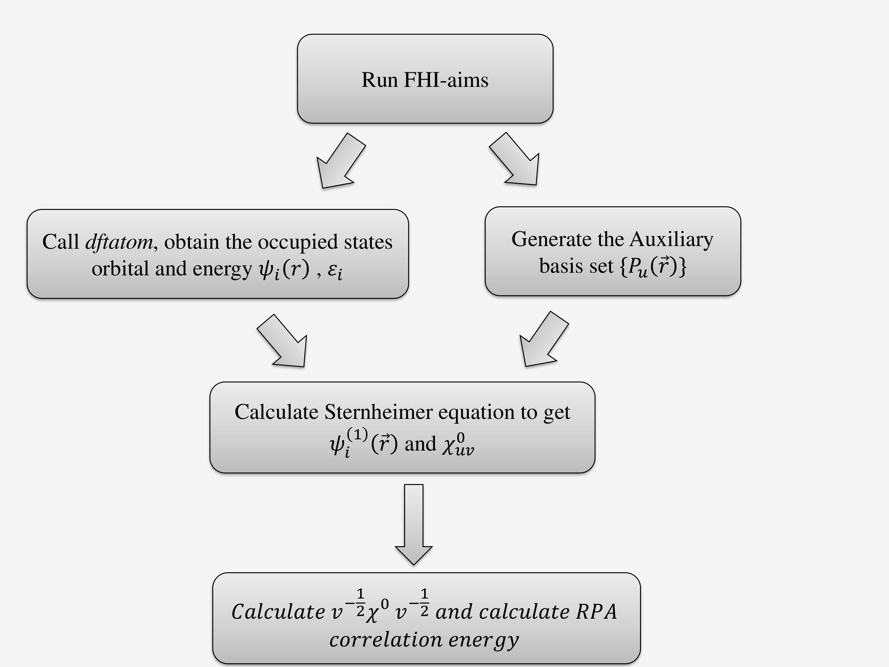
(a)

Figure 1: Major steps for computing the RI-RPA correlation energy using the Sternheimer approach.

4 Results

4.1 Converged RPA correlation energies for atoms

The basis-set dependence of the RI-RPA correlation energy obtained via the SOS scheme is reflected in two aspects: the size of the SPBS and that of ABS. The first determines the number of unoccupied states, which in turn determines the precision of the response function $\chi^{0}({\mathbf{r}},{\mathbf{r}^{\prime}},i\omega)$ in real space; the second determines the rank of the response function matrix, which governs how well $\chi^{0}({\mathbf{r}},{\mathbf{r}^{\prime}},i\omega)$ is represented in a matrix form. Naturally, the completeness of the ABS also affects the calculated results, which is usually referred to as the RI errors. In FHI-aims, the ABFs are generated according to the automatic procedure as described in Ref. 34 and Ref. 38. Within this procedure, the number of ABFs are controlled by two parameters: the highest angular momentum of the ABFs, $max\_l\_{aux}$, and a threshold $\eta_{orth}$ which is used in the Gram-Schmidt orthonormalization procedure to remove the redundancy of the “on-site” pair products of radial functions of AOs. In the tests below, we chose $max\_l\_{aux}=6$, and $\eta_{orth}=10^{-4}$, which works rather well for the SOS scheme, i.e., the RI error is vanishing small. We test two types of basis sets: NAO-VCC-nZ ² for NAOs and aug-cc-pVXZ for ^{1, 39} for GTOs, and check their convergence behavior for computing the RI-RPA correlation energy in both the SOS and Sternheimer schemes.

For the reference numbers adopted in this work, the “hard-wall cavity” approach as developed in Ref. ⁴⁰ is used, which has been demonstrated to yield highly converged RPA correlation energies for closed-shell atoms ⁴¹. Within this approach, the atom is placed in a cavity subject to a hard-wall confining potential imposed at a finite but large radius $R_{\text{max}}$. The radial KS equation is then solved on an one-dimensional dense grid mesh, yielding series of eigenstates characterized by principal quantum number $n$ and angular momentum quantum number $l$. These states consist in a systematic representation of the unoccupied space. Indeed, employing the thus obtained dense eigenstates in the SOS scheme, one can attain highly converged RPA correlation energies for atoms ⁴¹. In addition to $R_{\text{max}}$, other convergence parameters in this approach are $n_{max}$ and $l_{max}$ denoting the highest principal and angular momentum quantum numbers, respectively. Note that $n_{max}$ is typically of the order of a few hundreds, to achieve sub-mHa convergence in all-electron RPA correlation energy for each angular momentum $l$. Thus the total number of unoccupied states in this approach is huge and it is difficult to extend it to molecular systems. In Ref. ⁴¹, the reported RPA correlation energies are calculated on top of the KS reference of the optimized effective potential (OEP) at the exact exchange level (denoted as RPA@OEPx). To facilitate the comparison to the RPA results in this work, the “hard-wall cavity” approach is used here on top of the LDA starting point.

In Fig. 2, the RPA correlation energy of the Ne atom are presented as a function of the basis set size for both the SOS and Sternheimer schemes. We emphasize again that, in the Sternheimer scheme, one only uses the ABS generated using the SPBS labelled in the $x$ axis, rather than using the SPBS to expand the KS orbitals. Panel (a) and (b) of Fig. 2 present the convergence behavior for NAOs (NAO-VCC-$n$Z with $n=2$-5) and GTOs (aug-cc-pVXZ with X$=$D, T, Q, 5, 6), respectively. The reference value here is computed using the above-mentioned “hard-wall cavity" approach with $l_{max}=6$ (to be consistent with $max\_l\_{aux}=6$ for the ABS), $n_{max}=300$ and $R_{max}=10$ Bohr. From Fig. 2, one can clearly see that the RPA correlation energies based on the Sternheimer equation are much lower than their counterparts yielded by the SOS scheme, and can quickly converge to the reference value (up to 1 mHa) marked by horizontal dashed line, when the basis set increases from 2Z to 5Z for NAOs (Panel a). Similar convergence behavior is observed for GTOs from DZ to 6Z (Panel b). Remarkably, the RPA correlation energy obtained from the Sternheimer scheme using the 2Z-generated ABS is even lower than those obtained from the conventional SOS scheme using the largest NAO-VCC-5Z or aug-cc-pV6Z basis sets. It should be understood that the difference between the RPA correlation energies given by the two schemes reflects the incompleteness error of the SPBS, while the difference between the results based on the Sternheimer equation and the reference values reflects the incompleteness error of the ABS. In Fig. 3, these two types of BSIEs are further compared. It can be seen that, with the increase of the basis set size, the errors incurred by the SPBS and the ABS are both decreasing, but the error from the incompleteness of SPBS is dominating, and does not converge to zero even with the largest available NAO or GTO basis sets. As clearly shown in this session, invoking the Sternheimer approach to compute numerically accurate first-order wave functions can eliminate the major source of BSIEs in RI-RPA calculations.

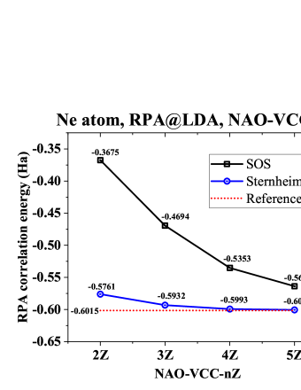
(a)

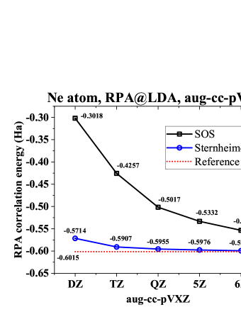
(b)

Figure 2: The RI-RPA correlation energy for the Ne atom as a function of the basis set size as obtained from the SOS and Sternheimer schemes. Results in panel (a) and (b) are calculated using NAO (NAO-VCC-nZ) and GTO (aug-cc-pVXZ) basis sets, respectively. The red dash line marks the reference result obtained using the “hard-wall cavity” approach ⁴¹.

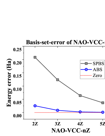
(a)

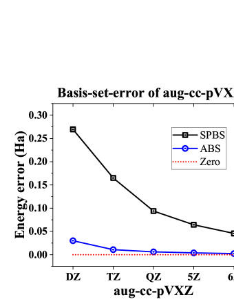
(b)

Figure 3: Two types of basis set incompleteness errors as a function of the basis size for both NAOs (panel a) and GTOs (panel b). Black squares indicate the difference between the RPA correlation energies for the Ne atom as obtained from the SOS and Stermheimer schemes ($E_{c}^{RPA-SOS}(n)-E_{c}^{RPA-Sternheimer}(n)$); the blue circles indicate the difference between the energies obtained from Sternheimer scheme and the reference value ($E_{c}^{RPA-Sternheimer}(n)-E_{c}^{RPA-ref}$).

Next, we look at the RPA correlation energies as obtained by the SOS and Sternheimer schemes for other elements with atomic numbers from 2 to 18, and compare the obtained results to the reference values as obtained using the “hard-wall cavity" approach ⁴¹.

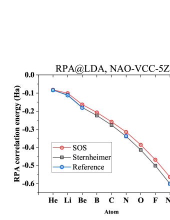
(a)

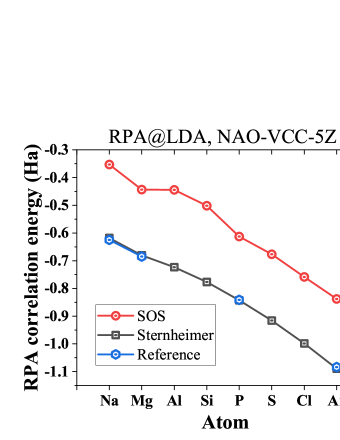
(b)

Figure 4: RPA correlation energies for atoms from He to Ar. The SOS results are obtained using the NAO-VCC-5Z basis set and the Sternheimer results are obtained using the ABS generated from NAO-VCC-5Z.

As is shown in Fig. 4, for all atoms, the RPA correlation energies obtained from the Sternheimer scheme are very close to the corresponding reference results, when they are available. In contrast, similar to the Ne atom case, the RPA correlation energies obtained using the conventional SOS scheme are appreciably above the reference results, except for He. This trend gets more pronounced for heavier elements in the third row of the periodic table (Panel b). The series of results presented in Fig. 4 confirm the efficacy of the Sternheimer scheme.

4.2 Further analysis: First-order density in real space

The significant difference between the RPA correlation energies yielded by the SOS and Sternheimer schemes is due to their different underlying density response function matrices $\chi^{0}_{\mu,\nu}$, which can be further traced back to the difference in the first-order density $n^{(1)}({\mathbf{r}})$ as obtained by the two schemes – denoted as $\Delta n^{(1)}({\mathbf{r}})$ below. It will be instructive to visualize $\Delta n^{(1)}({\mathbf{r}})$, which will then signify what is missing in the existing AO basis sets to accurately represent $n^{(1)}({\mathbf{r}})$. This will hopefully provide us a guidance for further improving the existing basis sets for correlated calculations.

Naturally, the shape of $n^{(1)}({\mathbf{r}})$, and hence that of $\Delta n^{(1)}({\mathbf{r}})$ depend on the actual applied perturbation. We found that for a spherically symmetric atomic system, the angular distributions of the first-order density and the perturbed Hamiltonian are always the same. Therefore, we only need to pay attention to the radial distribution of the first-order density difference.

As a test example, we add a $Y^{0}_{1}-type$ (i.e. $p_{z}$-type) perturbative potential to the Ar atom, and evaluate the difference in $n^{(1)}({\mathbf{r}})$ yielded by the two schemes. Here, the SPBS used in the SOS scheme is NAO-VCC-5Z, a rather large basis set in practical calculations. The radial part of $\Delta n^{(1)}({\mathbf{r}})$ and that of the applied perturbative potential are plotted in Fig. 5. In the upper, middle, and lower panels of Fig. 5, three different shapes of the perturbative potentials (different $p$-type radial ABFs), together with the resultant radial distributions of $\Delta n^{(1)}({\mathbf{r}})$ are plotted. It can be seen that, although the detailed behavior of $\Delta n^{(1)}({\mathbf{r}})$ depends on the applied disturbance, there are some common features: First, the error in the first-order density yielded by the SOS method roughly occurs in the region between 0 to 0.5 Bohr around the nucleus. Second, the radial distribution of $\Delta n^{(1)}({\mathbf{r}})$ is similar under different perturbations, with a peak near the nucleus. We also tested other ($s$, $d$, or $f$) types of perturbations, and the resultant $\Delta n^{(1)}({\mathbf{r}})$ show similar behavior as that illustrated in Fig. 5. The insights gained from the behavior of $\Delta n^{(1)}({\mathbf{r}})$ is instructive for developing complementary AOs to mitigate the BSIE for molecular and condensed materials. Research along this direction goes beyond the scope of the present paper and will be explored in the future work.

(a)

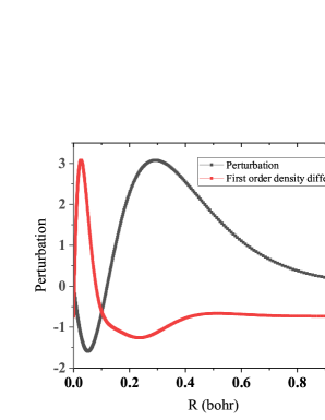
(b)

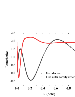
(c)

Figure 5: First order density differences $\Delta n^{(1)}({\mathbf{r}})$ of Ar atom under $p$-type perturbations with different radial shapes .

4.3 Optimization of ABFs

As demonstrated above, The RI-RPA correlation energy obtained using the Sternheimer scheme is free of SPBS error, but still depends on the quality of the employed ABS to represent the non-interacting response function $\chi^{0}$. In Ref. 42, it is pointed out that the Coulomb-metric RI-RPA correlation energy is variational, meaning that it is lower-bounded by the true RPA correlation energy that is free of the RI errors. In other words, by systematically increasing the variational space of the ABFs, the RI error of RI approximation decreases, and the RI-RPA correlation energy should in principle gradually converge to the true energy that is free of any BSIE.

Here we show that the variational property of RI-RPA can be exploited to generate optimized ABFs, picked up from a large pool of candidate functions. The candidate ABFs adopted here still have the form of a radial function multiplied by spherical harmonics, but for simplicity are restricted to hydrogen-like functions. The shape of hydrogen-like functions is controlled by the principal and angular quantum numbers, and by the effective charge $Z$ of the nucleus, i.e.,

$$R_{nl}(r)=\sqrt{\left(\frac{2Z}{na}\right)^{3}\frac{(n-l-1)!}{2n(n+l)!}}\left(\frac{2Zr}{na}\right)^{l}L_{n-l-1}^{2l+1}\left(\frac{2Zr}{na}\right)\mathrm{e}^{-Zr/(na)}\,,$$ (30)

where $L_{n-l-1}^{2l+1}$ in upper equation represents the associated Laguerre polynomial. The optimization procedure adopted here follows that used in Ref. 2. Namely, during the optimization process, we add trial hydrogen-like functions from a large pool of candidate functions one by one, and each time observe how the obtained RI-RPA correlation energy change with the effective charge $Z$. The one that yields the largest drop of the obtained energy will be picked up and added to the existing ABS, until a pre-set accuracy is reached.

Due to the orthogonality of the spherical harmonic functions, the ABFs with different angular momenta are independent of each other, and hence we optimize the ABFs belonging to different angular momentum channels separately. The convergence criterion of ABF optimization for each angular momentum is set to be $10^{-4}$ Ha, under which the size of the ABS is not too large, yet maintaining a high accuracy level. So far, we have optimized the ABFs following the above-described procedure for elements of atomic numbers from 2 to 18. Below, these newly optimized ABSs are denoted as “ABS-opt”. In Table 1, the optimized ABSs are compared with the standard ABSs generated by the automatic on-the-fly procedure ³⁴ with the NAO-VCC-4Z basis set, in terms of both their size and the obtained RI-RPA correlation energies. It can be seen that, compared to the standard ABSs generated using the NAO-VCC-4Z, the number of basis functions in the newly optimized ABS is less, yet yielding better (variationally lower) RPA correlation energies for all elements. This study suggests a promising way to create pre-optimized ABSs, which may become advantageous for general molecular or solid-state calculations.

Table 1: Comparison of the size of two types of ABSs and the corresponding RPA correlation energies obtained from the Sternheimer scheme. “ABS(NAO-4Z)” denotes the standard ABS generated via the automatic procedure ³⁴ with NAO-VCC-4Z ² basis set; “ABS-opt” denotes the ABS generated using the variational optimization procedure described in this section, containing exclusively “hydrogen-like" functions. $N_{aux}$ denotes the number of auxiliary function.

Atom	$N_{aux}$		$E_{c}^{RPA}$ (Ha)
	ABS(NAO-4Z)	ABS-opt	ABS (NAO-4Z)	ABS-opt
He	143	98	-0.0833	-0.0830
Li	226	143	-0.1087	-0.1102
Be	234	177	-0.1786	-0.1788
B	276	211	-0.2229	-0.2232
C	266	238	-0.2748	-0.2753
N	280	234	-0.3372	-0.3372
O	254	234	-0.4102	-0.4109
F	284	259	-0.4970	-0.4983
Ne	280	278	-0.5963	-0.5968
Na	362	298	-0.6137	-0.6202
Mg	368	276	-0.6751	-0.6795
Al	388	281	-0.7166	-0.7213
Si	400	295	-0.7724	-0.7744
P	381	306	-0.8341	-0.8373
S	384	306	-0.9063	-0.9091
Cl	395	322	-0.9876	-0.9909
Ar	379	313	-1.0792	-1.0808

4.4 RPA correlation energies based on the eigenspectrum of $\chi^{0}v$

As demonstrated above, empowered by the Sternheimer method, as long as high-quality ABS is available, accurate RPA correlation energy can be calculated. However, for heavy elements, we do not have NAO-VCC-$n$Z basis sets and hence no corresponding ABSs can be generated at the moment. Of course, one can in principle create optimized ABSs according to the procedure described in Sec. 4.3. However, for heavy elements, the optimization can get rather expensive and tedious. How to deal with this situation? In fact, as is shown in Ref. ²², based on the Steinheimer equation, it is possible to compute accurate RPA correlation energies without invoking an ABS.

From Eq. 1, one may realize that the RPA correlation energy can be readily computed once the eigenspectra of the operator $\chi^{0}(i\omega)v$ are determined for a set of frequency grid points. In terms of a set of ABFs, $\chi^{0}(i\omega)v$ is represented as a matrix; one can obtain the eigenspectrum of $\chi^{0}(i\omega)v$ by diagonalizing the matrix. Alternatively, utilizing the Sternheimer equation, one can employ the power iteration method ⁴³ to determine the eigenspectrum of the operator $\chi^{0}(i\omega)v$ iteratively, in terms of which the RPA correlation energy can be obtained, without the need of constructing a high-quality ABS.

The machinery of the power iteration method works as follows: One starts with an initial trial wave function $\left|\varphi\right\rangle$, which, without losing generality for atoms, also has the form of a radial function times spherical harmonics,

$$\varphi(\bm{r})=\varphi(r)Y_{L}^{M}(\theta,\phi)$$ (31)

Then, applying the operator $\chi^{0}(i\omega)v$ to $\left|\varphi\right\rangle$, one can obtain the first-order density $\Delta n(\bm{r})$ by solving Sternheimer equation. Formally, one has

$$\chi^{0}v\left|\varphi\right\rangle=\Delta n\,,$$ (32)

which physically corresponds to the first-order change of the density of KS system induced by an “external” potential $v|\varphi\rangle$, which is nothing but the Hartree potential associated with $\varphi(\bm{r})$,

$$\langle{\mathbf{r}}|v\varphi\rangle=\int\frac{\varphi({\mathbf{r}^{\prime}})}{|{\mathbf{r}}-{\mathbf{r}^{\prime}}|}d{\mathbf{r}^{\prime}}\,.$$ (33)

Thus, $\Delta n$ in Eq. 32 can be readily computed by solving the Sternheimer equation with $\langle{\mathbf{r}}|v\varphi\rangle$ taken as the perturbation. As discussed in the previous section, for a spherical atom, the first-order density has the same angular distribution of the perturbed Hamiltonian, namely,

$$\Delta n(\bm{r})=\Delta n(r)Y_{L}^{M}(\theta,\phi)\,.$$ (34)

We then normalize the resultant $\Delta n(r)$ and take it as the “perturbation” of the next iteration. Repeating this process, one will attain a right eigenvector of the operator $\chi^{0}(i\omega)v$ and the corresponding eigenvalue. Next, taking another trial function and orthogonalize it against the eigenvectors that have already been found, one will get the next eigenvalue and eigenvector. The eigenspectrum of $\chi^{0}(i\omega)v$ is negative definite, and bounded below zero. By performing such operation repeatedly, one can gradually retrieve the eigenspectrum of the operator $\chi^{0}(i\omega)v$ belonging to a given angular momentum channel $L$, up to a pre-set threshold for the eigenvalues. It is worth noting that the different values of $M$ correspond to degenerate eigenvectors, owing to the spherical symmetry of atoms. So the degeneracy of each eigenvalue belonging to a given angular momentum channel $L$ is 2$L$+1. By varying the angular momentum $L$ and repeating the above iteration process, one can obtain the entire eigenspectrum of any angular momentum channel, at any imaginary frequency point. As mentioned above, once the eigenspectrum of $\chi^{0}(i\omega)v$ is attained, the RPA correlation energy can be trivially calculated via Eq. 1. Moreover, this method does not depend on any basis set. The convergence behavior of this “basis-free” approach can be examined from two aspects: First, the convergence of the RPA correlation energy with the increase of the number of eigenvalues for a fixed angular momentum channel $L$. Second, the convergence behavior of RPA correlation energy with respect to the maximum value of the angular momentum $L_{max}$. A detailed analysis of the convergence behavior with respect to these two factors is given in Appendix D, using Kr atom and Ar atom as examples.

Because no pre-constructed basis set is needed, we can compute the RPA correlation energy for any element. Another important point is that the eigenspectrum obtained via the power iteration method is given systematically from large to small in terms of absolute values, and their contributions to the RPA correlation energy are hence getting gradually smaller. Therefore, for a given $L$, one can make the calculation arbitrarily accurate by increasing the number of eigenvalues included. Here, we set the precision threshold to be 0.1 meV, i.e., further eigenvalues will be discarded if the change of the RPA correlation energy is below 0.1 meV. Regarding the convergence behavior with respect to $L_{max}$, we observe a rather good $1/L_{max}^{3}$ of the calculated RPA correlation energy for large $L_{max}$ (cf. Appendix D), which is consistent with the early analysis based on the quantum chemistry correlated methods ^{44, 45}. Such a behavior allows one to readily extrapolate the results to the limit of $L_{max}\rightarrow\infty$. In Table LABEL:tab:2 we present the obtained all-electron RPA@LDA correlation energies for atoms of species from H to Kr (1-36). Results for both $L_{max}=14$ and extrapolated $L_{max}\rightarrow\infty$ are reported, in comparison to the reference results obtained using the “hard-wall cavity” method ⁴¹ with $L_{max}=14$, available only for closed-shell and half-filled open-shell atoms. We note that the “basis-free” approach for calculating the RPA correlation energy described here is very similar to that discussed in Ref. ²², but there only results for a few closed-shell atoms are presented.

Table LABEL:tab:2 shows that the Sternheimer scheme together with the power iteration method yields results that are in excellent agreement with the reference results obtained using the “hard-wall cavity” method ⁴¹. In particular, the results presented in the third column and the reference results presented in the fourth column are both obtained with $L_{max}=14$ and hence directly comparable. For closed-shell atoms, the difference between the results yielded by these two rather different approaches are $\sim$ 50 meV or smaller. For half-filled open-shell atoms, the difference is noticeably larger (at the level of 0.1 eV), and this is mostly because spin degeneracy is assumed in the Sternheimer-based calculations (due to the restriction imposed by the “dftatom” code ³⁵), where spin-polarized calculations were done in case of the “hard-wall cavity” method. Test RPA calculations based on the usual SOS scheme as implemented in FHI-aims indicates that the RPA correlation energies obtained with spin-polarized and spin-degenerate DFA configurations have differences at the level of 0.1 eV for most open-shell atoms. Finally, the difference between the second and third columns in Table LABEL:tab:2 reflects the deviation between the result obtained with a large but finite $L_{max}$ from the extrapolated $L_{max}\rightarrow\infty$ result. The deviation is only about a couple of meV for light elements and increases to more than 0.1 eV for the heavier (fourth-row) elements. Such a difference has no relevance for any binding energy calculations that are of physical interest, but nevertheless the second column of Table LABEL:tab:2 provides numerically highly converged all-electron atomic RPA correlation energies for all chemical elements from 1 to 36, which can serves as reference values for any future studies along this line.

Table 2: RPA@LDA correlation energies (in eV) for atoms with atomic numbers 1-36. The first column presents the extrapolated ($L_{max}\rightarrow\infty$) basis-free results, and the second column contains results obtained with $L_{max}=14$. The reference results in the third column are obtained using the “hard-wall cavity” method ⁴¹ with $L_{max}=14$.

Atom	RPA-basis-free ($L_{max}\rightarrow\infty$)	$L_{max}=14$	Reference
H	-0.568	-0.568	-0.569
He	-2.287	-2.286	-2.288
Li	-3.045	-3.044	-3.078
Be	-4.950	-4.948	-4.952
B	-6.159	-6.156	/
C	-7.612	-7.607	/
N	-9.348	-9.341	-9.241
O	-11.403	-11.393	/
F	-13.801	-13.789	/
Ne	-16.567	-16.552	-16.517
Na	-17.239	-17.222	-17.211
Mg	-18.929	-18.911	-18.857
Al	-20.115	-20.095	/
Si	-21.610	-21.587	/
P	-23.381	-23.355	-23.219
S	-25.415	-25.385	/
Cl	-27.709	-27.675	/
Ar	-30.269	-30.231	-30.281
K	-31.757	-31.716	/
Ca	-34.191	-34.147	/
Sc	-36.479	-36.431	/
Ti	-37.306	-37.252	/
V	-40.914	-40.854	/
Cr	-44.348	-44.280	/
Mn	-46.031	-45.958	/
Fe	-48.966	-48.885	/
Co	-52.091	-52.002	/
Ni	-55.410	-55.313	/
Cu	-61.451	-61.343	/
Zn	-62.649	-62.533	/
Ga	-63.003	-62.882	/
Ge	-63.940	-63.813	/
As	-65.297	-65.164	/
Se	-66.997	-66.858	/
Br	-68.992	-68.845	/
Kr	-71.291	-71.136	/

5 Conclusions

The convergence of explicit correlated methods in terms of atomic orbitals to the CBS limit is a challenging problem. Practical calculations rely on the availability of high-quality hierarchical basis sets and the extrapolation to the CBS limit based on empirical rules. In this work, we demonstrate that, by solving the Sternheimer equation on a dense radial grid, one is able to obtain numerically fully converged RI-RPA correlation energy for atoms. It is shown that the RPA correlation energies obtained with the biggest available atomic orbitals within the usual SOS scheme are still quite far from the converged results obtained using the Sternheimer scheme. The BSIE of the RI-RPA scheme is analyzed in terms of both the SPBS and ABS, and it is found that the major source of BSIE arises from the SPBS whereas the error due to ABS is marginal. Our scheme also offers a recipe to variationally construct optimal ABS for RI-RPA calculations, and provides insights about the deficiencies of existing AO basis sets. The latter is important for designing improved AO basis sets.

The numerical technique we developed for solving the Sternheimer equation for atomic RPA calculations can be extended to diatomic molecules and to other correlated methods like $GW$. Works along these lines are ongoing. Advances in such numerical techniques will not only provide unprecedented benchmark values for atom and diatomic systems, but also provide valuable guidance for developing high-quality AO (in particular NAO) basis sets for correlated calculations for general molecular and extended systems.

Data availability

Data that support the findings of this study are available from the corresponding author upon reasonable request.

We thank Christoph Friedrich and Volker Blum for very helpful discussions. This work was funded by the National Key Research and Development Program of China (Grant No. 2022YFA1403800), the National Natural Science Foundation of China (Grant Nos. 12188101 and 12134012), and the Max Planck Partner Group project on Advanced Electronic Structure Methods.

Appendix A Frequency-dependent linear response theory

The basic frequency-dependent linear response theory has been discussed in the literature (e.g., cf. Ref. ³²). For the paper to be self-contained, we present below a derivation of the frequency-dependent linear response theory to set up the basis equations and the notational system. We start with the single-particle KS Hamiltonian of the system,

$$H^{(0)}(\bm{r})=-\frac{1}{2}\bigtriangledown^{2}+V_{eff}(\bm{r})$$ (35)

where $V_{eff}(\bm{r})$ usually contains three terms,

$$V_{eff}(\bm{r})=V_{ext}(\bm{r})+V_{h}(\bm{r})+V_{xc}(\bm{r})\,.$$ (36)

Consider a time-dependent perturbed external potential $V^{(1)}(\bm{r},t)$ that has the following form,

$$V^{(1)}(\bm{r},t)=V^{(1)}(\bm{r})(e^{i\omega t}+e^{-i\omega t})e^{\eta t}$$ (37)

where $\omega$ represents the frequency of the monochromatic perturbation, and $\eta=0^{+}$, indicating that the perturbation is adiabatically switched on from the remote past $t=-\infty$. Now the full Hamiltonian is given by

$$H(\bm{r},t)=H^{(0)}(\bm{r})+V^{(1)}(\bm{r},t)$$ (38)

whose eigenfunctions can be generally written in the form of perturbation expansion,

$$\psi_{i}(\bm{r},t)=(\psi^{(0)}_{i}(\bm{r})+\psi^{(1)}_{i}(\bm{r},t)+\psi^{(2)}_{i}(\bm{r},t)+\dots)e^{i(E^{(0)}_{i}+E^{(1)}_{i}(t)+E^{(2)}_{i}(t)+\dots)t}\,.$$ (39)

In particular, $\psi^{(0)}_{i}(\bm{r})$ satisfies the stationary (zeroth-order) Schrödinger equation:

$$H^{(0)}(\bm{r})\psi^{(0)}_{i}(\bm{r})=E^{(0)}_{i}\psi^{(0)}_{i}(\bm{r})\,.$$ (40)

In linear response theory, one discards second- and higher-order terms, arriving at

$$\psi_{i}(\bm{r},t)\approx(\psi^{(0)}_{i}(\bm{r})+\psi^{(1)}_{i}(\bm{r},t))e^{i(E^{(0)}_{i}+E^{(1)}_{i}(t))t}$$ (41)

Here, the expression of $E^{(1)}_{i}(t)$ is akin to the stationary perturbation theory,

$$E^{(1)}_{i}(t)=\int_{-\infty}^{t}{\rm d}{t^{\prime}}\left\langle\psi_{i}^{(0)}\right|V^{(1)}(t^{\prime})\left|\psi_{i}^{(0)}\right\rangle$$ (42)

In the linear response regime, the first-order wave function should have the same time dependence as the perturbation,

$$\psi^{(1)}_{i}(\bm{r},t)=(\psi^{(1)}_{i,+\omega}(\bm{r})e^{i\omega t}+\psi^{(1)}_{i,-\omega}(\bm{r})e^{-i\omega t})e^{\eta t}\,.$$ (43)

Now we need to find the differential equation that $\psi_{i,\pm\omega}^{(1)}$ satisfies. To this end, we start from the time-dependent Schrödinger equation,

$$i\frac{d\psi_{i}(\bm{r},t)}{dt}=(H^{(0)}(\bm{r})+V^{(1)}(\bm{r},t))\psi_{i}(\bm{r},t)\,,$$ (44)

and by approximating $\psi_{i}(\bm{r},t)$ by its first-order expansion (Eq.  41), the left-hand side ($l.h.s.$) and right-hand side ($r.h.s.$) of Eq.  44 can be separately expressed as,

$$l.h.s =i\frac{d((\psi^{(0)}_{i}(\bm{r})+\psi^{(1)}_{i}(\bm{r},t)e^{i(E^{(0)}_{i}+E^{(1)}_{i}(t))t})}{dt}$$ (45)

$$r.h.s =(H^{(0)}(\bm{r})+V^{(1)}(\bm{r},t))\left[(\psi^{(0)}_{i}(\bm{r})+\psi^{(1)}_{i}(\bm{r},t)e^{i(E^{(0)}_{i}+E^{(1)}_{i}(t))t}\right]$$

Using Eqs. 42 and 43, one can get,

$$\tilde{E}^{(1)}_{i}\psi^{(0)}_{i}(\bm{r})(e^{i\omega t}+e^{-i\omega t})+E^{(0)}_{i}(\psi^{(1)}_{i,+\omega}(\bm{r})e^{i\omega t}+\psi^{(1)}_{i,-\omega}(\bm{r})e^{-i\omega t})+$$ (46)

$$(-\omega+i\eta)\psi^{(1)}_{i,+\omega}(\bm{r})e^{i\omega t}+(\omega+i\eta)\psi^{(1)}_{i,-\omega}(\bm{r})e^{-i\omega t}$$

$$= H^{(0)}(\bm{r})(\psi^{(1)}_{i,+\omega}(\bm{r})e^{i\omega t}+\psi^{(1)}_{i,-\omega}(\bm{r})e^{-i\omega t})+V^{(1)}(\bm{r})\psi^{(0)}_{i}(\bm{r})(e^{i\omega t}+e^{-i\omega t})\,,$$

where $\tilde{E}^{(1)}_{i}$ is given by,

$$\tilde{E}^{(1)}_{i}=\left\langle\psi_{i}^{(0)}\right|V^{(1)}\left|\psi_{i}^{(0)}\right\rangle\,.$$ (47)

In the derivation of Eq. 46, the second-order terms are discarded, whereas the zero-order term is eliminated by using Eq. 40.

Equation 46 can be reorganized into two equations, utilizing the linear independence of $e^{i\omega t}$ and $e^{-i\omega t}$,

$$(H^{(0)}(\bm{r})-E^{(0)}_{i}+\omega-i\eta)\psi^{(1)}_{i,+\omega}(\bm{r})=(\tilde{E}^{(1)}_{i}-V^{(1)}(\bm{r}))\psi^{(0)}_{i}(\bm{r})$$ (48)

$$(H^{(0)}(\bm{r})-E^{(0)}_{i}-\omega-i\eta)\psi^{(1)}_{i,-\omega}(\bm{r})=(\tilde{E}^{(1)}_{i}-V^{(1)}(\bm{r}))\psi^{(0)}_{i}(\bm{r})$$ (49)

In fact, Eq. 48 and Eq. 49 are essentially the same equation,

$$(H^{(0)}(\bm{r})-E^{(0)}_{i}+\omega-i\eta)\psi^{(1)}_{i,\omega}(\bm{r})=(\tilde{E}^{(1)}_{i}-V^{(1)}(\bm{r}))\psi^{(0)}_{i}(\bm{r})$$ (50)

which is referred to as the frequency-dependent Sternheimer equation.

In RPA calculations, it is convenient to work with imaginary frequencies. To this end, one can analytically continue the frequency variable from real to imaginary domains, and Eq. 50 then becomes,

$$(H^{(0)}(\bm{r})-E^{(0)}_{i}+i\omega)\psi^{(1)}_{i,i\omega}(\bm{r})=(\tilde{E}^{(1)}_{i}-V^{(1)}(\bm{r}))\psi^{(0)}_{i}(\bm{r})\,.$$ (51)

This is the Eq. 13 in the main text we would like to derive.

Appendix B Derivation of radial Sternheimer equation

Starting from Eq. 13, the original frequency-dependent Sternheimer equation can be reduced to an one-dimensional radial equation. Here we show how this simplification is achieved. Using Eqs. 19-20, 22 and 24, the $l.h.s.$ and $r.h.s.$ of Eq. 13 become,

$$l.h.s. = (-\frac{1}{2}\nabla^{2}+V_{eff}(r)-\epsilon_{i}+i\omega)\left[\sum_{l^{\prime}m^{\prime}}u_{i\mu,l^{\prime}m^{\prime}}^{(1)}(r,i\omega)Y_{l^{\prime}}^{m^{\prime}}(\theta,\phi)\right]$$ (52)

$$r.h.s. = [\epsilon_{i}^{(1)}-V_{\mu}^{(1)}(r)Y_{L}^{M}(\theta,\phi)]u_{i,l}(r)Y_{l}^{m}(\theta,\phi)$$ (53)

In terms of spherical coordinates, the kinetic energy operator $-1/2\nabla^{2}$ can be decomposed into $-\frac{1}{2r}\frac{\partial^{2}}{\partial r^{2}}r+\frac{\widehat{L}^{2}}{2r^{2}}$. And using

$$\widehat{L}^{2}Y_{l^{\prime}}^{m^{\prime}}(\theta,\phi)=l^{\prime}(l^{\prime}+1)Y_{l^{\prime}}^{m^{\prime}}(\theta,\phi)\,,$$ (54)

Eq. 52 changes into

$$l.h.s.=\sum_{l^{\prime}m^{\prime}}Y_{l^{\prime}}^{m^{\prime}}(\theta,\phi)\left(-\frac{1}{2r}\frac{\partial^{2}}{\partial r^{2}}r+\frac{l^{\prime}(l^{\prime}+1)}{2r^{2}}+V_{eff}(r)-\epsilon_{i}+i\omega\right)u_{i\mu,l^{\prime}m^{\prime}}^{(1)}(r,i\omega)\,.$$ (55)

Multiplying both sides of the equation with $Y_{l^{\prime\prime}}^{m^{\prime\prime}}(\theta,\phi)$ and integrating with respect to the angular coordinates ${(\theta,\phi)}$, and further utilizing the orthogonality relationship between real spherical harmonic functions,

$$\int{\rm d}{\Omega}{Y_{l^{\prime}}^{m^{\prime}}}(\theta,\phi)Y_{l}^{m}(\theta,\phi)=\delta_{ll^{\prime}}\delta_{mm^{\prime}}\,.$$ (56)

one gets,

$$l.h.s. = \sum_{l^{\prime}m^{\prime}}\delta_{l^{\prime\prime}l^{\prime}}\delta_{m^{\prime\prime}m^{\prime}}\left(-\frac{1}{2r}\frac{\partial^{2}}{\partial r^{2}}r+\frac{l^{\prime}(l^{\prime}+1)}{2r^{2}}+V_{eff}(r)-\epsilon_{i}+i\omega\right)u_{i\mu,l^{\prime}m^{\prime}}^{(1)}(r,i\omega)$$ (57)

$$= \left(-\frac{1}{2r}\frac{\partial^{2}}{\partial r^{2}}r+\frac{l^{\prime\prime}(l^{\prime\prime}+1)}{2r^{2}}+V_{eff}(r)-\epsilon_{i}+i\omega\right)u_{i\mu,l^{\prime\prime}m^{\prime\prime}}^{(1)}(r,i\omega)$$

$$r.h.s. = [\epsilon_{i}^{(1)}\delta_{l^{\prime\prime}l}\delta_{m^{\prime\prime}m}-G_{l^{\prime\prime}Ll}^{m^{\prime\prime}Mm}V_{\mu}^{(1)}(r)]u_{i,l}(r)$$ (58)

$\epsilon^{(1)}_{i}$ in Eq. 15 is given by the Gaunt coefficient multiplied by a radial integral.

$$\epsilon_{i}^{(1)} =\left\langle\psi_{i}\right|V^{(1)}\left|\psi_{i}\right\rangle$$ (59)

$$=G_{lLl}^{mMm}\int{\rm d}{r}u_{i,l}^{*}(r)V_{\mu}^{(1)}(r))u_{i,l}(r)$$

Due to the existence of $\delta_{l^{\prime\prime}l}\delta_{m^{\prime\prime}m}$, the Gaunt coefficient can be moved outside the bracket, ending up with

$$r.h.s.=G_{l^{\prime\prime}Ll}^{m^{\prime\prime}Mm}[\epsilon_{i-radial}^{(1)}\delta_{l^{\prime\prime}l}\delta_{m^{\prime\prime}m}-V_{\mu}^{(1)}(r)]u_{i,l}(r)$$ (60)

Finally, by equating Eq. 57 and 60 and replacing$\left\{{l^{\prime\prime},m^{\prime\prime}}\right\}$ by $\left\{{l^{\prime},m^{\prime}}\right\}$, one obtains the desired radial Sternheimer equation given by Eq. 25.

Appendix C Solving the radial Sternheimer equation by finite-difference method

The radial Sternheimer equation (Eq. 25) is solved using finite-difference method, which is implemented in FHI-aims, whereby the radial wavefunctions are tabulated on a logarithmic grid,

$$r(i)=r_{min}*r_{inc}^{(i-1)}\,.$$ (61)

Such coordinates are more suitable for describing the wave functions near the nucleus, but uneven grids are not convenient for the implementation of finite-difference method. So we introduce coordinate transformation to convert logarithmic coordinate $r(i)$ to uniform coordinate $x(i)$, and the corresponding relationship is as follows,

$$x(i)=ln(r(i))=ln(r_{min})+(i-1)*ln(r_{inc})$$ (62)

$$\frac{d}{dr}=\frac{dx}{dr}\frac{d}{dx}=\frac{1}{r}\frac{d}{dx}=e^{-x}\frac{d}{dx}$$

The key issue is the treatment of second derivative in Eqs. 25 and 29. Introduce $f(r)=\sqrt{r}u^{(1)}(r)$, we can get,

$$\frac{1}{r}\frac{\partial^{2}}{\partial r^{2}}\,ru^{(1)}(r) =\frac{1}{r}\frac{\partial}{\partial r}\left(\frac{\partial}{\partial r}\sqrt{r}f(r)\right)$$ (63)

$$=\frac{1}{r^{2}}\frac{\partial}{\partial x}e^{-x}\frac{\partial}{\partial x}e^{\frac{1}{2}x}f(x)$$

$$=r^{-5/2}(f^{\prime\prime}(x)-\frac{1}{4}f(x))$$

On uniform grids, $f^{\prime\prime}(x)$ can be expressed as:

$$f^{\prime\prime}[x(i)]=\frac{f[x(i+1)]+f[x(i-1)]-2f[x(i)]}{\Delta x^{2}}$$ (64)

Therefore, the expression of the second-order differential equation (taking Eq. 25 as an example, and Eq. 29 is the same) on the grids is given as follows,

$$-\frac{1}{2}\frac{f[x(i+1)]+f[x(i-1)]-2f[x(i)]}{\Delta x^{2}}+\frac{(l^{\prime}+1/2)^{2}}{2}+r[x(i)]^{2}(V_{eff}[x(i)]-\epsilon_{i}+i\omega)f[x(i)]$$ (65)

$$= G_{l^{\prime}Ll}^{m^{\prime}Mm}r[x(i)]^{5/2}\left(\epsilon_{i-rad}^{(1)}\delta_{ll^{\prime}}\delta_{mm^{\prime}}-V_{\mu}^{(1)}[x(i)]\right)u_{i,l}[x(i)]$$

Equation LABEL:eq:finite_difference_radial_equation can be transformed into a linear system of equations $Af=B$. $A$ has the following tri-diagonal symmetric form:

$$A=\left(\begin{array}[]{cccc}\frac{1}{\Delta x^{2}}+\frac{(l^{\prime}+0.5)^{2}}{2}+r(1)^{2}(v_{eff}(1)-\epsilon_{i}+i\omega)&-\frac{1}{2\Delta x^{2}}&0&...\\ -\frac{1}{2\Delta x^{2}}&\frac{1}{\Delta x^{2}}+\frac{(l^{\prime}+0.5)^{2}}{2}+r(2)^{2}(v_{eff}(2)-\epsilon_{i}+i\omega)&-\frac{1}{2\Delta x^{2}}&...\\ 0&-\frac{1}{2\Delta x^{2}}&...&...\\ ...&...&...&...\end{array}\right)$$ (66)

Appendix D Convergence behavior analysis

D.1 Convergence behavior with respect to the eigenvalues of $\chi^{0}v$

In Sec. 4.4, we discussed how to calculate the RPA correlation energy in terms of the eigenspectrum of the $\chi^{0}v$ operator. Under a certain angular momentum truncation $L_{max}$, we can gradually increase the number of eigenvalues for each angular momentum channel, and monitor the convergence behavior of the RPA correlation energy. It should be noted that the eigenspectrum of $\chi^{0}v$ determined via the power iteration method is given in descending order in term of the absolute value of the eigenvalues, and hence the change in RPA correlation energy will become gradually smaller. We find that, if the change of the RPA correlation energy $\Delta E_{c}^{RPA}$ is less than 0.1 meV upon including one more eigenvalue, the RPA correlation energy can converge to within 1 meV. Taking the Kr atom as an example, we found that, starting from the 30th eigenvalue on, each eigenvalue contributes less than 0.1 meV to the RPA correlation energy. Figure 1 shows the cumulative contributions stemming from the $30th$ to $100th$ eigenvalues to the RPA correlation energy. As can be clearly seen, the cumulative energy error is below 1 meV by increasing the number of eigenvalues from 30 to 100. This means that the remaining error resulting from the convergence threshold we set (below 0.1 meV upon including one more eigenvalue) is minute.

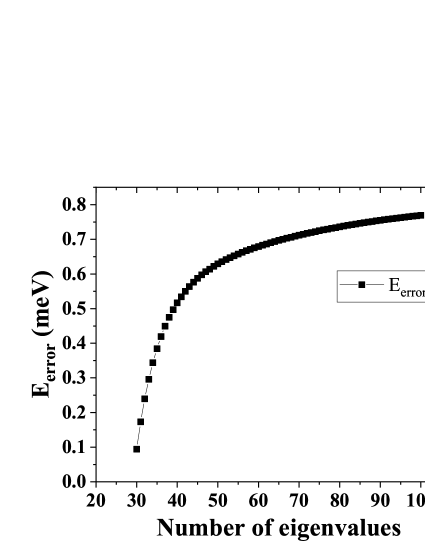
(a)

Figure 6: The change of the RPA correlation energy of the Kr atom by increasing the numbers of eigenvalues of $\chi^{0}v$ in the calculation. The figure shows that the cumulative change of the energy is below 1 meV when the number of eigenvalues increases from 30 to 100.

D.2 Convergence behavior with respect to $L_{max}$

Early analysis showed that the electron correlation energy for a spherical system converges as $1/L_{max}^{3}$ where $L_{max}$ is the highest angular momentum included in the calculation ^{44, 45}. Here, we show that the convergence of the RPA correlation energy with respect to $L_{max}$ also follows $1/L_{max}^{3}$ behavior for large $L_{max}$. An illustrating example is shown in Fig. 7 for the example of Ar atom.

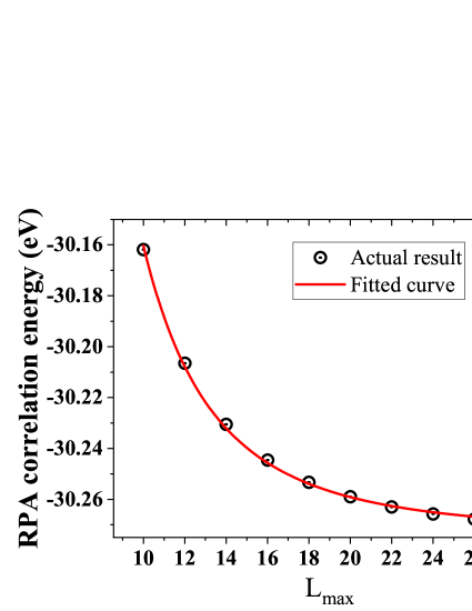
(a)

Figure 7: The convergence of the RPA@LDA correlation energy with respect to the highest angular momentum $L_{max}$ included in the calculation.

Based on this, we can establish the relationship between the RPA correlation energy under a certain $L_{max}$ truncation and that when $L_{max}$ approaches infinity,

$$E_{c}^{RPA}(L_{max})=E_{c}^{RPA}(L_{max}\rightarrow{\infty})+\frac{C}{L_{max}^{3}}$$ (67)

This means that we can fit data obtained with finite $L_{max}$, and obtain $E_{c}^{RPA}(L_{max}\rightarrow{\infty})$ from an extrapolation.

In Fig. 7, we presented the RPA correlation energy of Ar atom for $L_{max}$ from 10 to 28. The convergence with respect to the number of eigenvalues of $\chi^{0}v$ under each angular momentum follows the procedure described in Sec. D.1. We fitted the data according to the expression given in Eq. 67, and the fitted curve is shown in Fig. 7. The fitting coefficient of determination $R^{2}$ equals 0.99898, indicating that the fitted data is highly consistent with the fitting expression. The analytical expression obtained from the fitting is given by,

$$E_{c}^{RPA}(L_{max})=-30.27325+\frac{112.93756}{L_{max}^{3}}$$ (68)

Therefore, the estimated value of $E_{c}^{RPA}(L_{max}\rightarrow{\infty})$ is $-30.27325$ eV. If we just use three data at $L_{max}=10,12,14$, then the fitted result shows the estimated value of $E_{c}^{RPA}(L_{max}\rightarrow{\infty})$ is -30.26949 eV. So the error bars of fitting the results with these three data points are within 10 meV. The presented $L_{max}\rightarrow\infty$ results in Table LABEL:tab:2 are obtained by fitting the data points with $L_{max}=10,12,14$.

References

- T. H. Dunning 1989 T. H. Dunning, J. Gaussian basis sets for use in correlated molecular calculations. I. The atoms boron through neon and hydrogen. J. Chem. Phys. 1989, 90, 1007
- Zhang et al. 2013 Zhang, I. Y.; Ren, X.; Rinke, P.; Blum, V.; Scheffler, M. Numeric atom-centered-orbital basis sets with valence-correlation consistency from H to Ar. New J. of Phys. 2013, 15, 123033
- Helgaker et al. 1997 Helgaker, T.; Koch, W. K. H.; Noga, J. Basis-set convergence of correlated calculations on water. J. Chem. Phys. 1997, 106, 9639
- Eshuis et al. 2012 Eshuis, H.; Bates, J. E.; Furche, F. Electron Correlation Methods Based on the Random Phase Approximation. Theor. Chem. Acc. 2012, 131, 1084
- Ren et al. 2012 Ren, X.; Rinke, P.; Joas, C.; Scheffler, M. Random-phase approximation and its applications in computational chemistry and materials science. J. Mater. Sci. 2012, 47, 7447
- Zhang and Ren 2023 Zhang, I. Y.; Ren, X. Introduction to the Fifth-rung Density Functional Approximations: Concept, Formulation, and Applications. 2023, arXiv:2301.12119
- Jensen et al. 2017 Jensen, S. R.; Saha, S.; Flores-Livas, J. A.; Huhn, W.; Blum, V.; Goedecker, S.; Frediani, L. The Elephant in the Room of Density Functional Theory Calculations. The Journal of Physical Chemistry Letters 2017, 8, 1449–1457, PMID: 28291362
- Sternheimer 1951 Sternheimer, R. M. On Nuclear Quadrupole Moments. Phys. Rev. 1951, 84, 244
- Sternheimer 1954 Sternheimer, R. M. Electronic polarizabilities of ions from the Hartree-Fock wave functions. Physical Review 1954, 96, 951
- Sternheimer 1957 Sternheimer, R. M. Electronic polarizabilities of ions. Physical Review 1957, 107, 1565
- Sternheimer 1970 Sternheimer, R. M. Quadrupole polarizabilities of various ions and the alkali atoms. Physical Review A 1970, 1, 321
- Mahan 1980 Mahan, G. Modified Sternheimer equation for polarizability. Physical Review A 1980, 22, 1780
- Zangwill and Soven 1980 Zangwill, A.; Soven, P. Density-functional approach to local-field effects in finite systems: Photoabsorption in the rare gases. Physical Review A 1980, 21, 1561
- Mahan 1982 Mahan, G. Van der Waals coefficient between closed shell ions. The Journal of Chemical Physics 1982, 76, 493–497
- Andrade et al. 2007 Andrade, X.; Botti, S.; Marques, M. A. L.; Rubio, A. Time-dependent density functional theory scheme for efficient calculations of dynamic (hyper)polarizabilities. The Journal of Chemical Physics 2007, 126, 184106
- Gerratt and Mills 1968 Gerratt, J.; Mills, I. M. Force Constants and Dipole-Moment Derivatives of Molecules from Perturbed Hartree–Fock Calculations. I. The Journal of Chemical Physics 1968, 49, 1719–1729
- Baroni et al. 1987 Baroni, S.; Giannozzi, P.; Testa, A. Green’s-function approach to linear response in solids. Phys. Rev. Lett. 1987, 58, 1861–1864
- Baroni et al. 2001 Baroni, S.; de Gironcoli, S.; Corso, A. D.; Giannozzi, P. Phonons and related crystal properties from density-functional perturbation theory. Rev. Mol. Phys. 2001, 73, 515
- Gonze 1995 Gonze, X. Adiabatic density-functional perturbation theory. Phys. Rev. A 1995, 52, 1096–1114
- Wilson et al. 2008 Wilson, H. F.; Gygi, F.; Galli, G. Efficient iterative method for calculations of dielectric matrices. Physical Review B 2008, 78, 113303
- Wilson et al. 2009 Wilson, H. F.; Lu, D.; Gygi, F.; Galli, G. Iterative calculations of dielectric eigenvalue spectra. Physical Review B 2009, 79, 245106
- Nguyen and de Gironcoli 2009 Nguyen, H.-V.; de Gironcoli, S. Efficient calculation of exact exchange and RPA correlation energies in the adiabatic-connection fluctuation-dissipation theory. Physical Review B 2009, 79, 205114
- Umari et al. 2009 Umari, P.; Stenuit, G.; Baroni, S. Optimal representation of the polarization propagator for large-scale GW calculations. Phys. Rev. B 2009, 79, 201104
- Umari et al. 2010 Umari, P.; Stenuit, G.; Baroni, S. GW quasiparticle spectra from occupied states only. Phys. Rev. B 2010, 81, 115104
- Giustino et al. 2010 Giustino, F.; Cohen, M. L.; Louie, S. G. GW method with the self-consistent Sternheimer equation. Phys. Rev. B 2010, 81, 115105
- Nguyen et al. 2012 Nguyen, H.-V.; Pham, T. A.; Rocca, D.; Galli, G. Improving accuracy and efficiency of calculations of photoemission spectra within the many-body perturbation theory. Phys. Rev. B 2012, 85, 081101
- Betzinger et al. 2012 Betzinger, M.; Friedrich, C.; Görling, A.; Blügel, S. Precise response functions in all-electron methods: Application to the optimized-effective-potential approach. Physical Review B 2012, 85, 245124
- Betzinger et al. 2013 Betzinger, M.; Friedrich, C.; Blügel, S. Precise response functions in all-electron methods: Generalization to nonspherical perturbations and application to NiO. Physical Review B 2013, 88, 075130
- Betzinger et al. 2015 Betzinger, M.; Friedrich, C.; Görling, A.; Blügel, S. Precise all-electron dynamical response functions: Application to COHSEX and the RPA correlation energy. Physical Review B 2015, 92, 245101
- Gunnarsson and Lundqvist 1976 Gunnarsson, O.; Lundqvist, B. I. Exchange and correlation in atoms, molecules, and solids by the spin-density-functional formalism. Phys. Rev. B 1976, 13, 4274
- Langreth and Perdew 1977 Langreth, D. C.; Perdew, J. P. Exchange-correlation energy of a metal surface: Wave-vector analysis. Phys. Rev. B 1977, 15, 2884
- Marques et al. 2012 Marques, M. A.; Maitra, N. T.; Nogueira, F. M.; Gross, E. K.; Rubio, A. Fundamentals of time-dependent density functional theory; Springer, 2012; Vol. 837
- Talman 2011 Talman, J. D. Multipole expansions of orbital products about an intermediate center. International Journal of Quantum Chemistry 2011, 111, 2221–2227
- Ren et al. 2012 Ren, X.; Rinke, P.; Blum, V.; Wieferink, J.; Tkatchenko, A.; Sanfilippo, A.; Reuter, K.; Scheffler, M. Resolution-of-identity approach to Hartree–Fock, hybrid density functionals, RPA, MP2 and GW with numeric atom-centered orbital basis functions. New Journal of Physics 2012, 14, 053020
- Čertík et al. 2013 Čertík, O.; Pask, J. E.; Vackář, J. dftatom: A robust and general Schrödinger and Dirac solver for atomic structure calculations. Computer Physics Communications 2013, 184, 1777–1791
- Press et al. 2007 Press, W. H.; Teukolsky, S. A.; Vetterling, W. T.; Flannery, B. P. Numerical recipes 3rd edition: The art of scientific computing; Cambridge university press, 2007
- Klimeš et al. 2014 Klimeš, J. K.; Kaltak, M.; Kresse, G. Predictive GW calculations using plane waves and pseudopotentials. Phys. Phys. B 2014, 90, 075125
- Ihrig et al. 2015 Ihrig, A. C.; Wieferink, J.; Zhang, I. Y.; Ropo, M.; Ren, X.; Rinke, P.; Scheffler, M.; Blum, V. Accurate localized resolution of identity approach for linear-scaling hybrid density functionals and for many-body perturbation theory. New Journal of Physics 2015, 17, 093020
- Yousaf and Peterson 2009 Yousaf, K. E.; Peterson, K. A. Optimized complementary auxiliary basis sets for explicitly correlated methods: aug-cc-pVnZ orbital basis sets. Chemical Physics Letters 2009, 476, 303–307
- Jiang and Engel 2005 Jiang, H.; Engel, E. Second-order Kohn-Sham perturbation theory: Correlation potential for atoms in a cavity. The Journal of Chemical Physics 2005, 123, 224102
- Jiang and Engel 2007 Jiang, H.; Engel, E. Random-phase-approximation-based correlation energy functionals: Benchmark results for atoms. The Journal of chemical physics 2007, 127, 184108
- Eshuis et al. 2010 Eshuis, H.; Yarkony, J.; Furche, F. Fast computation of molecular random phase approximation correlation energies using resolution of the identity and imaginary frequency integration. The Journal of chemical physics 2010, 132, 234114
- Booth 2006 Booth, T. E. Power iteration method for the several largest eigenvalues and eigenfunctions. Nuclear science and engineering 2006, 154, 48–62
- Schwartz 1962 Schwartz, C. Importance of Angular Correlations between Atomic Electrons. Phys. Rev. 1962, 126, 1015
- Hill 1985 Hill, R. N. Rates of convergence and error estimation formulas for the Rayleigh-Ritz variational method. J. Chem. Phys. 1985, 83, 1173