CF-GODE: Continuous-Time Causal Inference for
Multi-Agent Dynamical Systems

Abstract.

Multi-agent dynamical systems refer to scenarios where multiple units (aka agents) interact with each other and evolve collectively over time. For instance, people’s health conditions are mutually influenced. Receiving vaccinations not only strengthens the long-term health status of one unit but also provides protection for those in their immediate surroundings. To make informed decisions in multi-agent dynamical systems, such as determining the optimal vaccine distribution plan, it is essential for decision-makers to estimate the continuous-time counterfactual outcomes. However, existing studies of causal inference over time rely on the assumption that units are mutually independent, which is not valid for multi-agent dynamical systems. In this paper, we aim to bridge this gap and study how to estimate counterfactual outcomes in multi-agent dynamical systems. Causal inference in a multi-agent dynamical system has unique challenges: 1) Confounders are time-varying and are present in both individual unit covariates and those of other units; 2) Units are affected by not only their own but also others’ treatments; 3) The treatments are naturally dynamic, such as receiving vaccines and boosters in a seasonal manner. To this end, we model a multi-agent dynamical system as a graph and propose a novel model called CF-GODE (CounterFactual Graph Ordinary Differential Equations). CF-GODE is a causal model that estimates continuous-time counterfactual outcomes in the presence of inter-dependencies between units. To facilitate continuous-time estimation, we propose Treatment-Induced GraphODE, a novel ordinary differential equation based on graph neural networks (GNNs), which can incorporate dynamical treatments as additional inputs to predict potential outcomes over time. To remove confounding bias, we propose two domain adversarial learning based objectives that learn balanced continuous representation trajectories, which are not predictive of treatments and interference. We further provide theoretical justification to prove their effectiveness. Experiments on two semi-synthetic datasets confirm that CF-GODE outperforms baselines on counterfactual estimation. We also provide extensive analyses to understand how our model works.

1. Introduction

Estimating counterfactual outcomes over time is critical to gaining causal understanding for many useful practical applications, such as how to distribute the limited vaccines in the early days to maximize protection over time (Medlock and Galvani, 2009), or how to design proper scheduling of medical treatments to optimize the patient recovery process (Bica et al., 2020). Randomized controlled trials (RCTs) are the gold standard for causal inference, but they can be cost-prohibitive and ethically challenging, particularly when considering the dynamical settings described above. Therefore, estimating counterfactual outcomes from observational data is the key approach to answering causal questions in real-world scenarios. Existing research on observational causal inference over time has begun by utilizing basic linear regression (Robins et al., 2000) and Gaussian processes (Xu et al., 2016) to capture the time-dependencies. Subsequently, advancements have been made by incorporating more advanced deep learning models such as recurrent neural networks (RNNs)  (Bica et al., 2020; Fujii et al., 2022) and Transformers  (Melnychuk et al., 2022).

Despite the progress, all aforementioned studies have relied on the assumption that units (e.g., people in the vaccine example) are independent of each other, i.e., each unit is solely influenced by its own treatment but not by others. In many realistic scenarios, however, this assumption is not valid. For instance, a person’s vaccination not only protects themselves but also those close to them. This type of setting is referred to as a multi-agent dynamical system (Gazi and Fidan, 2007), where units (also known as agents) interact with each other and evolve collectively over time. Many practical problems can be expressed as multi-agent dynamical systems, such as the long-term effects of vaccination where people mutually influence (Halloran and Hudgens, 2012), brain network signals in which the regions of interest (ROI) in a brain are associated (Yu et al., 2022; Cui et al., 2022), and molecular systems movements where the atoms are interconnected  (Durrant and McCammon, 2011). Prior approaches for causal inference over time are not applicable to multi-agent dynamical systems since they are not capable of handling the interconnections between units. In this paper, we propose to study this novel problem counterfactual estimation in multi-agent dynamical systems, which has received limited attention in the literature.

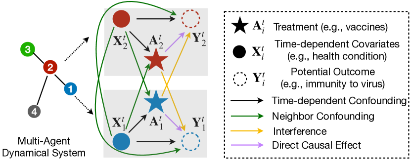
Figure 1. Causal graph at time $t$ in a multi-agent dynamical system. The causal variables are represented by shapes, while their relationships are distinguished by colors.

The dynamic and interrelated nature of multi-agent dynamical systems poses unique and nontrivial challenges to causal inference. We illustrate them along with Fig. 1. 1) Multi-source confounders. Confounders are variables that have an impact on both treatments and outcomes, leading to spurious correlations between them. Therefore, in observational data, the treatments are not balanced among units with different confounders values, resulting in biased counterfactual outcomes estimation. For example, old people are more likely to receive vaccines, but also face a higher risk of virus infection. If we train a standard supervised model using such imbalanced data, it may wrongly predict that vaccines may increase the infection risk for young people. In multi-agent dynamical systems, the confounders are multi-source, including time-dependent confounders and neighbor confounders. Time-dependent confounders refer to the fact that the confounders typically evolve over time and thus their impact on treatments and outcomes also changes dynamically (Platt et al., 2009; Bica et al., 2020). For instance, people’s health conditions change over time, affecting their likelihood of getting vaccinated and future health status. Neighbor confounders mean that a unit’s treatment and outcome could also be confounded by the covariates of its near units (neighbors) (Forastiere et al., 2021; Arbour et al., 2016), For example, if family members are in poor health, a unit may be more likely to receive a vaccine. Compared to the independent setting, neighbor confounders are additional confounding factors in multi-agent dynamical systems. 2) Imbalance of interference. As discussed in the previous example that vaccines protect not only a unit but also those in close proximity, the outcome of a unit can be influenced by others’ treatments in multi-agent dynamical systems. In causal language, this phenomenon is referred to as interference. Similar to the treatments, interference is affected by the covariates and thus is not balanced across the units in observational data (Forastiere et al., 2021). For instance, highly educated units are more likely to receive vaccines and typically have more highly educated friends. Therefore, they receive stronger protection through higher vaccination rates among their social networks. Such imbalanced interference causes additional bias in the estimation of counterfactual outcomes. 3) Continuous dynamics. In realistic applications, a multi-agent dynamical system is continuous in nature (Porter and Gleeson, 2014). However, most existing causal models are discrete, making them inappropriate for multi-agent dynamical systems. Modeling continuous-time observations (such as covariates and outcomes) and continuously estimating counterfactual outcomes over time remains an open challenge.

In this paper, we address the above challenges and study how to estimate continuous-time counterfactual outcomes, in presence of multi-source confounders and interference, in multi-agent dynamical systems. This is a novel, yet challenging and under-explored problem with valuable real-world applications.

To this end, we model a multi-agent dynamical system as a graph, where nodes represent units and edges capture their interactions. Inspired by recent achievements in graph ordinary differential equations (GraphODE) (Huang et al., 2020), we propose CF-GODE, a novel causal model that estimates continuous-time CounterFactual outcomes based on Graph Ordinary Differential Equations in multi-agent dynamical systems. Specifically, we use GraphODE as a backbone to model the continuous trajectory of each unit. However, in this case, traditional GraphODE can only model the pure dynamics of potential outcomes (Huang et al., 2020) and lacks the ability to incorporate additional inputs such as treatments, making it inappropriate for causal inference. To address this issue, in CF-GODE, we propose Treatment-Induced GraphODE, a new GraphODE model capable of handling treatments when predicting the future trajectory of potential outcomes. Treatment-Induced GraphODE uses graph neural networks (GNNs) (Kipf and Welling, 2017) to formulate its differential equations, which can effectively capture the mutual dependencies between units including neighbor confounders and interference. This advantage makes it a natural fit for counterfactual estimation in multi-agent dynamical systems. Then a latent representation is learned for each unit from its observations as the solution to Treatment-Induced GraphODE, which represents the continuous trajectory driven by treatments. The core of ensuring CF-GODE is a causal model is to deal with the aforementioned estimation bias caused by imbalanced treatments and interference in the observational data. We solve this issue via domain adversarial learning (Ganin et al., 2016; Wang et al., 2020), in which we treat the values of treatments (and interference) as domains and ensure the latent representation trajectories are invariant to them. We provide theoretical justification to demonstrate that the domain-adversarial balancing objective functions proposed in CF-GODE can effectively achieve the balancing goal, thereby removing bias in counterfactual estimation and ensuring that CF-GODE is causal.

We summarize our major contributions as follows: 1) We study how to estimate counterfactual outcomes in multi-agent dynamical systems, which is a novel yet challenging problem with useful practical implications. 2) We propose CF-GODE, a novel causal model for causal inference multi-agent dynamical systems based on GraphODE and domain-adversarial learning. 3) We provide theoretical analysis to show that CF-GODE is able to handle the imbalanced treatments and interference, ensuring unbiased counterfactual estimation. 4)We conduct extensive experiments to evaluate CF-GODE’s performance on counterfactual outcomes estimation in multi-agent dynamical systems.

2. Related Work

2.1. Causal Inference Over Time

The central challenge in estimating counterfactual outcomes in longitudinal settings is to remove the confounding bias from time-dependent covariates (Bica et al., 2020; Platt et al., 2009). The core solution to this in existing works is to cut off the association between covariates and the observed treatment assignments over time. To achieve this goal, statistical tools are widely used in traditional approaches. For example, marginal structural models (MSMs) (Robins et al., 2000) use inverse probability of treatment weighting (IPTW) (Rosenbaum and Rubin, 1983; Rosenbaum, 1987) to balance the distribution of covariates over time between unit groups that are assigned to different treatments. By doing so, treatment assignment can no longer be predicted from the balanced covariates, thus breaking their correlation. A later work (Lim et al., 2018) further enhances MSMs by using recurrent neural networks (RNNs) to learn the inverse probability of treatment weights (IPTWs), which is more capable of modeling sequential data. However, IPTW based tools can result in high variances in practice (Bica et al., 2020). To overcome this limitation, recent studies (Bica et al., 2020; Melnychuk et al., 2022) extend the representation learning based balancing approaches from static settings (Johansson et al., 2016; Yoon et al., 2018; Shalit et al., 2017; Yao et al., 2018) to dynamic settings. Specifically, counterfactual recurrent network (CRN) (Bica et al., 2020) uses RNNs to encode the time-varying covariates into latent embeddings over time, which are simultaneously optimized by two objectives: potential outcomes prediction and longitudinal distribution balancing w.r.t. treatment assignments. The learned balanced embeddings are not predictive of treatments, thus ensuring unbiased estimates of the potential outcomes. Since RNNs are less powerful in capturing long-range dependencies,  (Melnychuk et al., 2022) improves CRN by using Transformer (Vaswani et al., 2017) that preserves long-range dependencies between time-dependent confounders. Despite the progress, all the above models can only predict counterfactual outcomes in discrete timestamps. However, practical longitudinal sequences are continuous in nature.

Our work is most related to (Gwak et al., 2020; Bellot and Van Der Schaar, 2021; Seedat et al., 2022; De Brouwer et al., 2022), which estimate counterfactual outcomes in continuous dynamic settings using neural ordinary differential equations (ODEs) (Rubanova et al., 2019; Chen et al., 2018) or neural controlled differential equations (CDEs) (Kidger et al., 2020). Specifically,  (Seedat et al., 2022) infers continuous latent trajectories to represent the movement of potential outcomes and balance the distribution of this latent representation between treated and control groups via adversarial learning. However,  (Seedat et al., 2022) (and all aforementioned models) assume that units are mutually independent, which is usually not valid in many practical scenarios where the units affect each other, e.g., getting vaccinated provides long-term protection not only for oneself but also for their close ones. In contrast, our model is designed to estimate counterfactual outcomes in longitudinal settings where units are interdependent, i.e., the multi-agent dynamical systems.

2.2. Continuous Modeling With Neural Ordinary Differential Equations (ODEs)

Many dynamical systems are continuous in nature, which can be typically modeled using first-order ordinary differential equations (ODEs) (Porter and Gleeson, 2014). ODEs describe a system’s rate of change over time by a specific function, which is traditionally designed by domain experts (Qian et al., 2021), and more recently parameterized by neural networks (Rubanova et al., 2019; Chen et al., 2018; Massaroli et al., 2020), as a closed-form ODE function may be unknown for some complex real-world systems. Given initial states, the solution of a NeuralODE can be easily computed using any ODE solver, such as the Runge-Kutta method (Schober et al., 2019). In multi-agent dynamical systems, such as the spread of infectious disease among people, units often interact with one another, yet standard NeuralODEs do not explicitly model these interactions. Recent works have sought to address this limitation by representing the interactions among multiple units as graphs, and then utilizing graph neural networks (GNNs) (Kipf and Welling, 2017; Velickovic et al., 2018) to parameterize the ODE function (Huang et al., 2021, 2020; Zang and Wang, 2020; Poli et al., 2019). When predicting the dynamics of each unit, these GraphODE models not only take into account the unit’s own latent state but also aggregate the latent states of its connected units along the interaction graph, to effectively capture the mutual influence between them. However, GraphODE models are standard statistical methods and therefore lack the capability for causal inference. Instead, our model aims to address the unique challenges present in multi-agent dynamical systems, i.e., time-dependent confounders and network interference, in order to make counterfactual predictions.

3. Problem Setup

3.1. Problem Formulation

We study how to estimate counterfactual outcomes in the context of multi-agent dynamical systems, where the units engage in mutual interactions and evolve simultaneously over time. Throughout this paper, we use boldface uppercase letters to denote matrices or vectors, boldface uppercase letters with subscripts to signify elements of matrices or vectors, regular lowercase letters to represent values of variables, and calligraphic uppercase letters to indicate sets. We summarize all notations used in this paper in Appendix. A.4.

Formally, a multi-agent dynamical system can be represented by a dynamical graph $\mathcal{G}^{t}=(\mathcal{V},\mathcal{E}^{t})$, where $\mathcal{V}=\{v_{1},v_{2},...,v_{N}\}$ is the set of $N$ units (nodes) and $\mathcal{E}^{t}$ denotes the edge set at time $t$. An edge in $\mathcal{E}^{t}$ describes the intersection between the two units it connects at time $t$. In this paper, we present an early exploration of causal inference in multi-agent dynamical systems, and for the purpose of simplicity, we assume that the graph structure remains constant over time, i.e., $\mathcal{G}^{t}=\mathcal{G}$. Each unit is associated with time-varying variables, which are the causal quantities in our case. We introduce them together with the causal framework in the following.

We follow the longitudinal potential outcomes framework (Robins and Hernán, 2009; Rubin, 1978) to formalize the counterfactual outcome estimation as in (Bica et al., 2020; Seedat et al., 2022). The observational data $\left(\left(\mathbf{X}^{t},\mathbf{A}^{t},\mathbf{Y}^{t}\right)\cup\mathbf{V}\right)$ in a multi-agent dynamical system contains time-dependent covariates $\mathbf{X}^{t}$ (e.g., health condition), dynamical treatments $\mathbf{A}^{t}$ (e.g., vaccine allocation), and time-varying outcomes $\mathbf{Y}^{t}$ (e.g., immunity to infectious disease). It is worth noting that $\mathbf{Y}^{t}$ is essentially a part of $\mathbf{X}^{t}$. $\mathbf{V}$ denotes the static covariates of units such as ethnicity. Let the historical records of the multi-agent dynamical system up to time $t$ be represented by $\mathcal{H}^{t}=\{\mathbf{\bar{X}}^{t},\mathbf{\bar{A}}^{t},\mathbf{\bar{Y}}^{t},\mathbf{V}\}$, where $\mathbf{\bar{X}}^{t},\mathbf{\bar{A}}^{t},\mathbf{\bar{Y}}^{t}$ are all the $\mathbf{X}^{t^{-}},\mathbf{A}^{t^{-}},\mathbf{Y}^{t^{-}}$ until $t$ $(t^{-}\leq t)$, respectively. In causal inference, we are focused on understanding the potential outcomes $\mathbf{Y}^{t^{+}}(\mathbf{A}^{t^{+}}=a)$ that may occur in the future $(t^{+}>t)$ under a specific treatment $a$, which explains the impact of the treatment assignment on the dynamics of the system. Note that $a$ is a treatment trajectory that includes all treatments in the future time. Our goal is to estimate the future potential outcomes sequence driven by treatments in a multi-agent dynamical system, which is formalized as:

(1) $$\mathbb{E}\left(\mathbf{Y}^{t^{+}}(\mathbf{A}^{t^{+}}=a)\mid\mathcal{H}^{t},\mathcal{G}\right).$$

3.2. Causal Identification

The potential outcomes represented by $\mathbf{Y}^{t^{+}}(\mathbf{A}^{t^{+}}=a)$ are a causal quantity. To make it identifiable from observational data, we must adhere to the following necessary assumptions.

Assumption 1: Positivity (Overlap). The future treatment trajectory is probabilistic regardless of the historical observation, i.e., $0<P(\mathbf{A}^{t^{+}}=a\mid\mathcal{H}^{t})<1,\forall\mathcal{H}^{t}$.

Assumption 2: Consistency. Under the same treatment trajectory $a$, the potential outcome is equal to the observed outcomes, i.e., $\mathbf{Y^{t^{+}}}(\mathbf{A}^{t^{+}}=a)=Y^{t^{+}}$.

The above two assumptions are standard for longitudinal counterfactual estimation. To identify the potential outcomes, it is also necessary to assume that there are no unobserved confounders, i.e., the strong ignorability assumption. However, the typical sequential strong ignorability assumption (Bica et al., 2020; Seedat et al., 2022; Melnychuk et al., 2022; Lim et al., 2018) is not appropriate for multi-agent dynamical systems, because the graph structure $\mathcal{G}$ introduces extra graph confounders and interference. A plausible strong ignorability assumption for graphs is first introduced by (Forastiere et al., 2021) and later validated in studies such as (Ma and Tresp, 2021; Ma et al., 2022; Jiang and Sun, 2022). However, the assumption made in these works is limited to static settings. To address this, we extend it to longitudinal settings and adapt it to be applicable to multi-agent dynamical systems in the following.

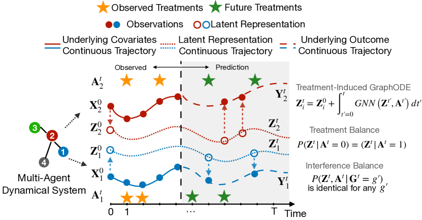
Figure 2. Overview of CF-GODE. The initial latent representation $\mathbf{\mathbf{Z}^{0}}$ is first learned from initial observations. Then the continuous latent representation trajectory $\mathbf{\mathbf{Z}^{t}}$ is learned as the solution to treatment-induced GraphODE, which is able to handle treatments as additional inputs. The graph neural network (GNN) based ODE function naturally models the mutual dependencies. The future potential outcomes can be decoded from $\mathbf{\mathbf{Z}^{t}}$ at any given time. To remove confounding bias, $\mathbf{\mathbf{Z}^{t}}$ is balanced with respect to 1) treatments, 2) interference when combined with corresponding treatments.

We first introduce a summary function, denoted as $g(\cdot)$, that captures the interference effects caused by the treatments of a node’s neighboring units in the graph as in (Forastiere et al., 2021). Formally, $\mathbf{G}_{i}^{t}=g(\mathbf{A}^{t}_{\mathcal{N}_{i}},\mathbf{A}^{t}_{\mathcal{N}_{-i}})$, where $\mathbf{A}^{t}_{\mathcal{N}_{i}}$ denotes the treatments of node $i$’s immediate neighbors, and $\mathbf{A}^{t}_{\mathcal{N}_{-i}}$ is the treatments of all the remaining node that are not directly connected to node $i$. We refer to $\mathbf{G}_{i}^{t}$ as interference summary. Here for simplicity, we adopt the assumption put forth in  (Forastiere et al., 2021; Arbour et al., 2016; Jiang and Sun, 2022) that a node is only influenced by the treatments of its immediate neighbors, i.e., $g(\mathbf{A}^{t}_{\mathcal{N}_{i}},\mathbf{A}^{t}_{\mathcal{N}_{-i}})=g(\mathbf{A}^{t}_{\mathcal{N}_{i}},\mathbf{A^{\prime}}^{t}_{\mathcal{N}_{-i}})=g(\mathbf{A}^{t}_{\mathcal{N}_{i}}),\forall\mathbf{A}^{t}_{\mathcal{N}_{-i}},\mathbf{A^{\prime}}^{t}_{\mathcal{N}_{-i}}$. $g(\cdot)$ can be instantiated using any aggregation functions or models. As in previous studies  (Forastiere et al., 2021; Ma and Tresp, 2021; Jiang and Sun, 2022), in this paper, we define $\mathbf{G}_{i}^{t}$ as the proportion of treated units in unit $i$’s neighbors, i.e., $\mathbf{G}_{i}^{t}\vcentcolon=\sum_{j\in\mathcal{N}_{i}}\frac{\mathbf{A}_{i}^{t}}{|N_{i}|}$. With $\mathbf{G}_{i}^{t}$, we present the strong ignorability assumption for multi-agent dynamical systems in the following:

Assumption 3: Strong Ignorability for Multi-Agent Dynamical Systems. Given the historical observations and the graph structure that describes the multi-agent dynamical system, the potential outcome trajectory is independent of the treatments and interference summary, i.e., $\mathbf{Y^{t^{+}}}(\mathbf{A}^{t^{+}}=a)\mathrel{\perp\mspace{-10.0mu}\perp}\mathbf{A}^{t^{+}},\mathbf{G}^{t^{+}}\mid\mathcal{H}^{t},\mathcal{G}.\forall a,t$.

With these three assumptions, the potential outcome trajectory Eq. (1) can be identifiable as:

$$\mathbb{E}\left(\mathbf{Y}^{t^{+}}(\mathbf{A}^{t^{+}}=a)\mid\mathcal{H}^{t},\mathcal{G}\right)$$

(2) $$=\mathbb{E}\left(\mathbf{Y}^{t^{+}}(\mathbf{A}^{t^{+}}=a)\mid\mathbf{A}^{t^{+}},\mathbf{G}^{t^{+}},\mathcal{H}^{t},\mathcal{G}\right)$$

(3) $$=\mathbb{E}\left(\mathbf{Y}^{t^{+}}\mid\mathbf{A}^{t^{+}},\mathbf{G}^{t^{+}},\mathcal{H}^{t},\mathcal{G}\right).$$

Eq. (2) is true because of assumption 3, while Eq. (3) holds under the assumption 2. The above causal identification enables us to estimate the potential outcomes in multi-agent dynamical systems using observational data. More specifically, we can train a machine learning model on observational data, which takes treatment trajectory $\mathbf{A}^{t^{+}}$, interference summary $\mathbf{G}^{t^{+}}$, historical observation $\mathcal{H}^{t}$ and graph $\mathcal{G}$ as inputs, and the observed (factual) outcome $\mathbf{Y}^{t^{+}}$ as targets, to predict the counterfactual outcomes given new treatment trajectories. Our proposed model CF-GODE is grounded in this and will be presented in detail in the subsequent section.

4. Proposed Model: CF-GODE

4.1. Overview

Our proposed CF-GODE is a causal model that predicts counterfactual outcomes in a multi-agent dynamical system by learning from observational data. We show an overview of our model in Fig. 2. Compared to most existing causal models designed for standard sequential settings that consider discrete time intervals and independent units (Bica et al., 2020; Melnychuk et al., 2022), multi-agent dynamical systems are more realistic and present two challenging properties: the dynamics are continuous in nature, and units are influenced by others. To address these, our proposed CF-GODE takes the advantage of recent breakthroughs in graph ordinary differential equations (GraphODE) (Huang et al., 2020, 2021) and extends it to handle treatments and interference, enabling continuous estimation of counterfactual outcomes in multi-agent dynamical systems. We refer to our ODE model as Treatment-Induced GraphODE (Sec. 4.2). The time-dependent confounders lead the distribution of covariates to be quite discrepant between units assigned to different treatments, resulting in high variances in counterfactual outcome estimation (Johansson et al., 2016; Shalit et al., 2017; Robins et al., 2000). This effect is further amplified by the imbalanced interference caused by the graph structure in multi-agent dynamical systems (Forastiere et al., 2021; Jiang and Sun, 2022). CF-GODE uses adversarial learning to alleviate this issue and guarantee unbiased estimates of counterfactual outcomes (Sec. 4.3).

4.2. Treatment-Induced GraphODE

To facilitate continuous-time counterfactual outcome estimation, we propose to learn a continuous latent trajectory $\mathbf{Z}_{i}^{t}$ for every node in multi-agent dynamical system that represents their movement. An ideal $\mathbf{Z}_{i}^{t}$ should possess two characteristics: 1) the ability to predict observed outcomes, and 2) not to be predictive of the received treatment or interference in observational data. We implement such a $\mathbf{Z}_{i}^{t}$ by a novel model called Treatment-Induced GraphODE, which empowers the recent GraphODE (Huang et al., 2020, 2021) to deal with treatment and interference for counterfactual outcomes estimation.

In a multi-agent dynamical system, the future outcomes of node $i$ might be affected by not only its own past movement and current treatment, but also the movements and interference from neighbors (e.g., a unit’s health condition and vaccination status have a significant impact on how likely others are to be infected). We model this process and formalize treatment-induced GraphODE as:

(4) $$\mathbf{Z}_{i}^{t}=\mathbf{Z}_{i}^{0}+\int_{t^{\prime}=0}^{t}\phi\left(\mathbf{Z}^{t^{\prime}},\mathbf{A}^{t^{\prime}}\right)dt^{\prime}.$$

In Eq. (4), $\mathbf{Z}^{t^{\prime}}$ and $\mathbf{A}^{t^{\prime}}$ denote the latent trajectory representations and treatments of all nodes in the multi-agent dynamical system, respectively. $\phi(\cdot)$ is the ODE function. To comprehensively capture the effects from node $i$ and its connected neighbors, we parameterize $\phi(\cdot)$ using graph neural networks (Kipf and Welling, 2017) with self-loops. $\mathbf{Z}_{i}^{0}$ is the initial state and can be encoded from the initial observations as $\mathbf{Z}_{i}^{0}=f(\mathbf{X}_{i}^{0},\mathbf{V}_{i})$, where $f(\cdot)$ is an encoder parameterized by neural networks. With $\mathbf{Z}_{i}^{0}$, we can obtain the $\mathbf{Z}_{i}^{t}$, which is the solution to treatment-induced GraphODE, by solving an ODE initial-value problem (IVP) in Eq. (4), formalized as:

(5) $$\mathbf{Z}_{i}^{0},\mathbf{Z}_{i}^{1}\cdots\mathbf{Z}_{i}^{T}=\text{ODESolve}\left(\phi,[\mathbf{Z}_{1}^{0},\mathbf{Z}_{2}^{0}\cdots\mathbf{Z}_{N}^{0}],\left(t_{0},t_{1}\cdots t_{T}\right)\right),$$

where $T$ is the number of timestamps for the evaluation of Eq. (5). With the solution latent trajectory $\mathbf{Z}_{i}^{t}$, we can then use a decoder $d_{\mathbf{Y}}(\cdot)$ to transform it to the predicted outcome $\hat{\mathbf{Y}}_{i}^{t}=d_{\mathbf{Y}}(\mathbf{Z}_{i}^{t})$. We also use neural networks to instantiate $d_{\mathbf{Y}}(\cdot)$. We compare the prediction $\hat{\mathbf{Y}}_{i}^{t}$ to ground-truths $\mathbf{Y}_{i}^{t}$ in all observed timestamps $\left(t_{0},t_{1}\cdots t_{T}\right)$ using a mean square error as objective, which is formalized as:

(6) $$L^{\langle Y\rangle}=\frac{1}{N}\frac{1}{T}\sum_{i}^{N}\sum_{t}^{T}\left(\hat{\mathbf{Y}}_{i}^{t}-\mathbf{Y}_{i}^{t}\right)^{2}.$$

4.3. Balancing via Adversarial Learning

In the observational data, the treatments applied to each unit $\mathbf{A}_{i}^{t}$ are affected by the time-dependent confounders present in the covariates (and thus in its latent representation trajectory $\mathbf{Z}_{i}^{t}$). Consequently, the distribution of latent representation trajectory is not balanced among units with different treatment assignments, i.e., $P(\mathbf{A}_{i}^{t}|\mathbf{Z}_{i}^{t})$ is not uniform, leading to high variances in the counterfactual outcome estimation (Johansson et al., 2016; Shalit et al., 2017). In the context of multi-agent dynamical systems, this effect is further exacerbated by the presence of imbalanced interference among units. This is because a unit’s interference is influenced by its covariates (also the latent representation) and treatments in the observational data, i.e., $P(\mathbf{G}_{i}^{t}|\mathbf{Z}_{i}^{t},\mathbf{A}_{i}^{t})$ is not uniform (Forastiere et al., 2021; Jiang and Sun, 2022; Ma and Tresp, 2021). Here we give an intuitive example of the imbalanced interference: consider that a highly educated person is more likely to be surrounded by other highly educated friends, who believe in science and are more likely to be vaccinated, thereby providing stronger protection for this person against infectious diseases, i.e., higher interference.

A sufficient condition to remove the above bias is to ensure that the distribution of latent representation trajectories is invariant to treatments, and when combined with the corresponding treatments, is interference-invariant (Shalit et al., 2017; Bica et al., 2020; Seedat et al., 2022; Forastiere et al., 2021; Jiang and Sun, 2022). This condition is formalized as $P(\mathbf{Z}^{t}|\mathbf{A}^{t}=0)=(\mathbf{Z}^{t}|\mathbf{A}^{t}=1)$ for treatment balancing, and $P(\mathbf{Z}^{t},\mathbf{A}^{t}|\mathbf{G}^{t}=g^{\prime})$ is identical for any given value of $g^{\prime}$ for interference balancing. The treatment $\mathbf{A}^{t}$ is binary and interference $\mathbf{G}^{t}$ is continuous as in (Forastiere et al., 2021; Jiang and Sun, 2022). Note that the aforementioned conditions are over the unit groups. This guarantees that the treatment cannot be inferred from the latent representation trajectory, and that the interference is not predictable when the treatment is combined with latent representation. We implement this balancing goal through domain adversarial learning (Ganin et al., 2016), in which the treatment is treated as binary domains and the interference is treated as continuous domains (Wang et al., 2020). Specifically, we use the gradient reversal layer proposed in (Ganin et al., 2016), denoted as $r(\cdot)$, to adversarially optimize the latent representation trajectory at every observed time, making it agnostic towards the treatments and interference.

Treatment Balancing. Formally, the predicted treatment is $\hat{\mathbf{A}}_{i}^{t}=d_{\mathbf{A}}\left(r(\mathbf{Z}_{i}^{t})\right)$, where the $d_{\mathbf{A}}$ is a neural network that attempts to recover the treatment from latent representation. The gradient reversal layer $r(\cdot)$ does nothing in the forward pass, but reverses the gradients in the back-propagation. This way, a min-max game is created in which $d_{\mathbf{A}}$ aims to minimize the treatment prediction loss, while the latent representation learner in treatment-induced GraphODE strives to maximize it, as formalized in the following:

(7) $$L^{\langle A\rangle}=\underset{d_{\mathbf{A}}^{j}}{\text{min}}\ \underset{f,\phi}{\text{max}}\frac{1}{N}\frac{1}{T}\sum_{i}^{N}\sum_{t}^{T}\sum_{j\in\{0,1\}}\mathds{1}_{(\mathbf{A}_{i}^{t}=j)}-\log\left(d_{\mathbf{A}}^{j}\left(r(\mathbf{Z}_{i}^{t})\right)\right),$$

where $d_{\mathbf{A}}^{j}$ represents the logits of $d_{\mathbf{A}}(\cdot)$ for predicting treatment $j$. We then provide a theoretical analysis to justify the capability of $L^{\langle A\rangle}$ to attain balanced representations in the following.

Theorem 1.

Let $j\in\{0,1\}$ be the binary treatment values, and let $N$ and $T$ denote the number of units and observed timestamp lengths, respectively. Let $P_{j}^{t}=P(\mathbf{Z}^{t}\mid\mathbf{A}^{t}=j)$, be the distribution of latent representation $\mathbf{Z}^{t}$ for the group of units with treatments $j$ at time $t$. Let $f$, $\phi$, $d_{\mathbf{A}}^{j}$ be the initial state encoder, the ODE function of treatment-induced GraphODE, and logits of predicting treatment $j$. The necessary and sufficient condition for the min-max game in Eq. (7) to be optimal is $P_{0}^{t}=P_{1}^{t},\forall t\in\left(t_{0},t_{1}\cdots t_{T}\right)$.

Theorem 1 suggests that the condition to obtain global optimum of Eq. (7) is $P(\mathbf{Z}^{t}|\mathbf{A}^{t}=0)=(\mathbf{Z}^{t}|\mathbf{A}^{t}=1)$. Therefore, by optimizing $L^{\langle A\rangle}$ in Eq. (7), we can ensure the latent representation trajectory $\mathbf{Z}^{t}$ is balanced with respect to treatments. In other words, $\mathbf{Z}^{t}$ is not predictive of $\mathbf{A}^{t}$. We prove Theorem 1 in Appendix. A.1.1.

Interference Balancing. The interference $\mathbf{G}_{i}^{t}$ is continuous, we thus adapt the continuous domain adversarial learning (Wang et al., 2020) to achieve the interference balancing. Similar to the binary case, we consider the continuous interference as continuous domains, and use the gradient reversal layer $r(\cdot)$ to build a min-max game on interference prediction as follows:

(8) $$L^{\langle G\rangle} =\underset{d_{\mathbf{G}}}{\text{min}}\ \underset{f,\phi}{\text{max}}\frac{1}{N}\frac{1}{T}\sum_{i}^{N}\sum_{t}^{T}\left(d_{\mathbf{G}}\left(r([\mathbf{Z}_{i}^{t},\mathbf{A}_{i}^{t}])\right)-\mathbf{G}_{i}^{t}\right)^{2}$$

where $d_{\mathbf{G}}$ is the interference predictor which is parameterized by neural networks, and $[\cdot,\cdot]$ is the concatenation operation. In the following, we also theoretically demonstrate that $L^{\langle G\rangle}$ is able to achieve the interference balancing objective.

Theorem 2.

Let $f$, $\phi$, $d_{\mathbf{G}}$ be the initial state encoder, the ODE function of treatment-induced GraphODE, and the interference predictor. The necessary and sufficient condition for min-max game in Eq. (8) to be optimal is $P(\mathbf{Z}^{t},\mathbf{A}^{t}|\mathbf{G}^{t}=g^{\prime})$ is identical for any $g^{\prime}$.

Theorem. 2 indicates that if $\mathbb{E}([\mathbf{Z}^{t},\mathbf{A}^{t}]\mid\mathbf{G}^{t})$ is identical for any $\mathbf{G}^{t}=g^{\prime}$, Eq. (8) achieves optimum. Therefore, it is sufficient to balance the combination of representations and treatments with respect to interference $\mathbf{G}^{t}$ by optimizing the objective function $L^{\langle G\rangle}$. We show the proof of Theorem 2 in Appendix. A.1.2.

4.4. Training of CF-GODE

Objective Function. The overall objective function of CF-GODE is formalized in the following:

(9) $$L=L^{\langle Y\rangle}+\alpha_{\mathbf{A}}L^{\langle A\rangle}+\alpha_{\mathbf{G}}L^{\langle G\rangle},$$

where coefficients $\alpha_{\mathbf{A}}$, $\alpha_{\mathbf{G}}$ are the strengths of the treatment balancing and interference balancing, respectively. By adversarially optimizing $L$, the latent representation trajectory $\mathbf{Z}_{i}^{t}$ is able to predict the outcome trajectory $\mathbf{Y}_{i}^{t}$ while remaining invariant to the treatments $\mathbf{A}_{i}^{t}$ and interference $\mathbf{G}_{i}^{t}$ (combined with treatments), which enables the unbiased counterfactual outcome estimation in multi-agent dynamical systems.

Alternative Training as Trade-Off. In practice, we find that directly training CF-GODE with the overall loss function $L$ may not be stable as $L^{\langle A\rangle}$ and $L^{\langle G\rangle}$ could hinder the ability of latent representation trajectory $\mathbf{Z}_{i}^{t}$ to predict the outcome. Therefore, we trade-off the training of CF-GODE in an alternative manner between $L$ and $L^{\langle Y\rangle}$, to ensure that $\mathbf{Z}_{i}^{t}$ is capable of predicting outcomes. Specifically, we switch the training iterations between $L$ and $L^{\langle Y\rangle}$ with a ratio of $K$, i.e., $\frac{Iter_{L}}{Iter_{L^{\langle Y\rangle}}}=K$, where $Iter$ means the number of training iterations and $K$ is a tunable hyperparameter. We elaborate on the training procedure in Appendix. A.2.

5. Experiments

5.1. Experimental Settings

Dataset. In observational data, we only have factual outcomes but not counterfactual outcomes. Therefore, we use semi-synthetics data to evaluate CF-GODE as in (Ma et al., 2022; Guo et al., 2020; Veitch et al., 2019). That is, we use two real graphs Flickr and BlogCatalog (Guo et al., 2020; Chu et al., 2021; Ma et al., 2021) and use a Pharmacokinetic-Pharmacodynamic (PK-PD) model (Goutelle et al., 2008) to simulate the continuous trajectory of treatments and potential outcomes (Bica et al., 2020; Seedat et al., 2022). The data simulation mimics the vaccine example in the real world. We introduce the data simulation process in detail in Appendix. A.3.

Metric. We focus on counterfactual outcomes estimation in this paper, which is a continuous value. Therefore, we use mean square errors (MSE) as our metric to evaluate the performance of our model, which is formalized as $MSE:=\frac{1}{N}\frac{1}{T}\sum_{i}^{N}\sum_{t}^{T}\left(\hat{\mathbf{Y}}_{i}^{t}-\mathbf{Y}_{i}^{t}\right)^{2}$.

Baselines. The scope of our model is in continuous-time causal inference, therefore we compare CF-GODE with the following baselines: CDE (Kidger et al., 2020): Ordinary differential equations with external inputs to adjust the continuous trajectory. GraphODE (Huang et al., 2020) Ordinary differential equations model with graph neural networks (GNNs) based ODE functions. TE-CDE (Seedat et al., 2022): the state-of-the-art model for continuous-time counterfactual outcomes estimation based on neural controlled differential equations (NeuralCDE).

Implementation. The parameters of CF-GODE are set as follows: the dimension of latent representations is $64$; the ODE solver is the Euler method; the balancing degrees are $\alpha_{\mathbf{A}}=\alpha_{\mathbf{G}}=0.5$. For training hyperparameters, the learning rate is $0.0001$; the default alternative training ratio $K$ is $4$. We train the model $5000$ epochs and select the best model according to the performance on the validation set. The parameters are optimized by Adam (Kingma and Ba, 2015). We run all experiments on a Lambda Labs instance with one A100 GPU.

Table 1. Counterfactual outcomes estimation errors on two datasets. “BC” is the abbreviation of the BlogCatalog dataset. The errors are broken down in x-step future estimation ($x\in[1,2,3,4,5]$). MSE errors are reported. The best results are in boldface and the second best results are underlined. CF-GODE-N is the variant of our model without any balancing; CF-GODE-T means balance only w.r.t. treatments; CF-GODE-I denotes balance only w.r.t. interference.

Dataset	Model	1-step	2-step	3-step	4-step	5-step	Overall
Flickr	CDE	0.134$\pm$0.015	0.164$\pm$0.017	0.198$\pm$0.021	0.237$\pm$0.023	0.281$\pm$0.026	0.203$\pm$0.205
	GraphODE	0.237$\pm$0.013	0.276$\pm$0.010	0.313$\pm$0.016	0.347$\pm$0.018	0.379$\pm$0.021	0.310$\pm$0.016
	TE-CDE	0.189$\pm$0.025	0.216$\pm$0.021	0.246$\pm$0.027	0.281$\pm$0.041	0.326$\pm$0.063	0.252$\pm$0.031
	CF-GODE-N	0.089$\pm$0.006	0.102$\pm$0.007	0.114$\pm$0.009	0.126$\pm$0.010	0.139$\pm$0.012	0.114$\pm$0.008
	CF-GODE-T	0.058$\pm$0.017	0.066$\pm$0.020	0.075$\pm$0.023	0.084$\pm$0.027	0.098$\pm$0.036	0.076$\pm$0.025
	CF-GODE-I	0.069$\pm$0.007	0.080$\pm$0.008	0.091$\pm$0.009	0.103$\pm$0.011	0.115$\pm$0.012	0.092$\pm$0.009
	CF-GODE	0.056$\pm$0.009	0.060$\pm$0.009	0.067$\pm$0.009	0.070$\pm$0.010	0.077$\pm$0.012	0.065$\pm$0.010
BC	CDE	0.255$\pm$0.120	0.324$\pm$0.178	0.407$\pm$0.263	0.515$\pm$0.383	0.640$\pm$0.549	0.427$\pm$0.296
	GraphODE	0.195$\pm$0.018	0.223$\pm$0.023	0.251$\pm$0.028	0.280$\pm$0.033	0.309$\pm$0.040	0.252$\pm$0.028
	TE-CDE	0.316$\pm$0.086	0.351$\pm$0.089	0.399$\pm$0.093	0.493$\pm$0.137	0.725$\pm$0.351	0.457$\pm$0.127
	CF-GODE-N	0.167$\pm$0.012	0.188$\pm$0.015	0.209$\pm$0.018	0.228$\pm$0.023	0.246$\pm$0.028	0.207$\pm$0.019
	CF-GODE-T	0.139$\pm$0.015	0.154$\pm$0.019	0.172$\pm$0.025	0.189$\pm$0.027	0.202$\pm$0.031	0.171$\pm$0.023
	CF-GODE-I	0.164$\pm$0.016	0.188$\pm$0.020	0.210$\pm$0.024	0.232$\pm$0.029	0.253$\pm$0.035	0.209$\pm$0.025
	CF-GODE	0.148$\pm$0.015	0.166$\pm$0.019	0.186$\pm$0.023	0.205$\pm$0.025	0.229$\pm$0.029	0.186$\pm$0.021

5.2. Can CF-GODE Deliver Accurate Estimations of Counterfactual Outcomes in Multi-Agent Dynamical Systems?

We compare CF-GODE to three lines of models: 1) Continuous-time dynamical prediction models CDE and GraphODE. Note that these baselines are not causal models since they only preserve the dynamical statistical associations. 2) Continuous-time causal inference model TE-CDE. But it is not capable of capturing the mutual dependencies between units in multi-agent dynamical systems. 3) Variants of CF-GODE. We consider three variants: CF-GODE-N means there is no any balancing ($\alpha_{\mathbf{A}}=\alpha_{\mathbf{G}}=0$); CF-GODE-T denotes balancing only w.r.t. treatments ($\alpha_{\mathbf{A}}=1$, $\alpha_{\mathbf{G}}=0$); CF-GODE-I means balancing only w.r.t. interference ($\alpha_{\mathbf{A}}=0$, $\alpha_{\mathbf{G}}=1$). For a multi-agent dynamical system with $N$ nodes and length-$A$ treatment trajectories, the total number of possible treatments for all nodes is $O(A\cdot 2^{N})$. Therefore, it is intractable to enumerate all treatment combinations. To this end, we randomly flip $50\%$ of all observed treatments in each experiment. We estimate five-step (timestamp) ahead counterfactual outcomes and report estimation errors in Table. 1. Generally, CF-GODE and the variants outperform the baselines by substantial margins. It is noteworthy that, despite being a causal model, TE-CDE performs clearly worse than the family of CF-GODE, because it ignores the mutual influence between units. This underscores our motivation to address this unique challenge in multi-agent dynamical systems. We also note CF-GODE-N is generally the weakest estimator among all variants, confirming the effectiveness of our proposed balancing objectives.

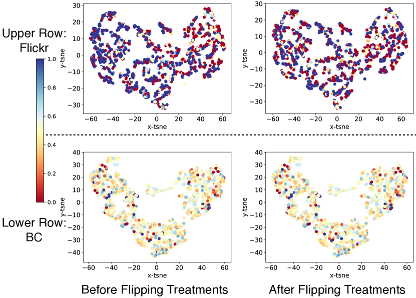
Figure 3. T-SNE projections of latent representations “before” (factual) and “after” (counterfactual) flipping the treatments. Each point represents a unit’s latent representation. The points are colored by the units’ corresponding interference. Upper row: Flickr dataset; Lower Row: BlogCatalog dataset.

Why Does CF-GODE-T Show Superior Performance Than CF-GODE on BlogCatalog Dataset? On BlogCatalog dataset, we observe that balancing solely with respect to treatments (CF-GODE-T) yields the lowest estimation errors, even outperforming balancing both treatments and interference (CF-GODE). To understand this phenomenon, we project all units’ latent representations $\mathbf{Z}^{t}$ into 2-D embeddings using T-SNE (Van der Maaten and Hinton, 2008) and color these 2-D points by their corresponding interference in Fig. 3. Specifically, we compare the units’ interference before and after flipping the treatments. Compared to Flickr, we notice that in BlogCatalog 1) the latent representations are already comparatively more balanced before flipping the treatments, and 2) the units’ interference does not change significantly after flipping the treatments. This suggests that balancing solely with respect to treatments might be sufficient in the BlogCatalog dataset. Actually, since we use the same data simulation protocol for Flickr and BlogCatalog, this difference in interference distribution is expected to be caused by their distinct graph structures. Specifically, the average and standard derivation of node degrees of the two datasets are Flickr: $2.0\pm 1.7$; BlogCatalog: $30.7\pm 25.1$. Intuitively, the interference of high degrees nodes is more resistant to flipping a random portion of their neighbors, which is pretty common among nodes in BlogCatalog. We provide further breakdown studies to better understand how node degrees affect counterfactual outcomes estimation in Sec. 5.5.

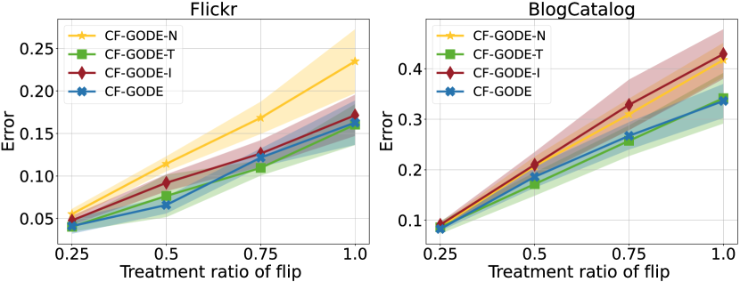
Figure 4. Counterfactual outcomes estimation errors w.r.t. the percentage of units in the graph whose treatments are flipped. Left: Flickr dataset; Right: BlogCatalog dataset.

5.3. How Does CF-GODE Respond to The Flipping of Counterfactual Treatments?

In the above experiments, the default treatment flipping ratio is set at $50\%$. It’s intriguing to investigate how CF-GODE reacts to different flipping ratios, as this would indicate the degree of difference between factual and counterfactual outcomes in terms of treatments. To this end, we set the flip ratio as $[25\%,50\%,75\%,100\%]$, and present the results of CF-GODE and its variants under these settings in Fig. 4. As expected, all models perform worse as the flip ratio increases, since the counterfactual treatments diverge further from the observed factual treatments. However, we observe that with balancing objectives, the error of CF-GODE increases generally slowly, highlighting the need for balancing objectives.

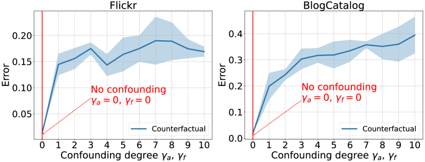
Figure 5. Counterfactual outcomes estimation errors w.r.t. 11 different confounding degrees $\gamma_{a}$ and $\gamma_{f}$. Note $\gamma_{a}$ and $\gamma_{f}$ are set as the same values in each experiment. The red line points to the “no confounding bias” setting ($\gamma_{a}=\gamma_{f}=0$).

5.4. How Does CF-GODE Respond to Different Confounding Degrees?

In data simulation, we use coefficients $\gamma_{a}$, $\gamma_{f}$ to control the degree of the time-dependent and neighbor confounding bias. With larger values of these coefficients, the confounding bias is more severe, leading to increasingly imbalanced data. To study how CF-GODE works under varying confounding degrees, we set $\gamma_{a}=\gamma_{f}=\gamma$, where $\gamma\in[0,1,2,3,4,5,6,7,8,9,10]$, and present the counterfactual outcomes estimation errors of CF-GODE under these conditions in Fig.5. The errors increase as the confounding bias becomes more severe, but the rate of increase is relatively smooth, particularly on Flickr dataset. This implicates CF-GODE’s robustness against high degree confounding bias. Additionally, CF-GODE produces low errors when there is no confounding bias ($\gamma_{a}=\gamma_{f}=0$), which demonstrates the compatibility of CF-GODE with such settings.

5.5. How Does Graph Structure Impact Counterfactual Outcomes Estimation?

As discussed in Sec. 5.2, the graph structure affects CF-GODE’s performance on counterfactual outcomes estimation. To gain deeper insights into this phenomenon, we break down the estimation errors on BlogCatalog dataset according to node degrees in Table. 2. Interestingly, we find that CF-GODE’s counterfactual estimation errors decrease as the node degrees become higher. Intuitively, this might also be because the interference of high-degree nodes is more stable. However, in this paper, we do not have a theoretical understanding of the relationships between estimation errors and node degrees. We leave this line of research in future study.

Table 2. The breakdown of counterfactual outcomes estimation errors by units (nodes) degrees in BlogCatalog dataset.

Degree	$\#$Nodes	Percentage$\%$	Error
(0,5]	176	10.2	0.243$\pm$0.337
(5,10]	185	10.6	0.235$\pm$0.344
(10,20]	389	22.5	0.216$\pm$0.296
(20,30]	312	18.0	0.218$\pm$0.314
(20,30]	200	11.5	0.221$\pm$0.295
(30,40]	165	9.5	0.195$\pm$0.284
(40,50]	98	5.7	0.176$\pm$0.269
$>$50	207	12.0	0.187$\pm$0.261

5.6. Can CF-GODE Be Generalized to New Multi-Agent Dynamical Systems?

Standard counterfactual outcome estimations are typically conducted on units whose factual outcomes have been observed. However, the estimation of the potential outcomes on new multi-agent dynamical systems is also of great importance. For instance, to predict the effects of an initial vaccine distribution strategy for a new community. To assess CF-GODE’s ability to generalize to new systems, i.e., new graphs, we split the original graph into three subgraphs, denoted as training/validation/testing graphs (details in Appendix. A.3). We train our model on the training graph and evaluate its potential outcome estimation on the testing graph. We report the results in Table. 3. We note that the performance of CF-GODE and the variants on new graphs are also generally better than baselines, which is consistent with the estimation of the counterfactual outcomes within the same graph (Sec. 5.2). This demonstrates our model’s generalizability to new multi-agent dynamical systems.

Table 3. Generalization errors of potential outcomes prediction for new multi-agent dynamical systems (new graphs) on two datasets. “BC” is the abbreviation of the BlogCatalog dataset. The errors are broken down in x-step future estimation ($x\in[1,2,3,4,5]$). MSE errors are reported. The best results are in boldface and the second best results are underlined. CF-GODE-N is the variant of our model without any balancing; CF-GODE-T means balance only w.r.t. treatments; CF-GODE-I denotes balance only w.r.t. interference.

Dataset	Model	1-step	2-step	3-step	4-step	5-step	Overall
Flickr	CDE	0.134$\pm$0.017	0.166$\pm$0.022	0.201$\pm$0.026	0.241$\pm$030	0.285$\pm$0.034	0.205$\pm$0.025
	GraphODE	0.209$\pm$0.010	0.243$\pm$0.012	0.275$\pm$0.015	0.306$\pm$0.018	0.335$\pm$0.022	0.274$\pm$0.014
	TE-CDE	0.193$\pm$0.023	0.221$\pm$0.021	0.251$\pm$0.027	0.285$\pm$0.040	0.328$\pm$0.061	0.256$\pm$0.030
	CF-GODE-N	0.087$\pm$0.06	0.099$\pm$0.008	0.111$\pm$0.009	0.122$\pm$0.010	0.134$\pm$0.011	0.111$\pm$0.008
	CF-GODE-T	0.057$\pm$0.014	0.064$\pm$0.016	0.072$\pm$0.018	0.081$\pm$0.022	0.092$\pm$0.029	0.738$\pm$0.020
	CF-GODE-I	0.071$\pm$0.007	0.083$\pm$0.008	0.096$\pm$0.009	0.109$\pm$0.010	0.122$\pm$0.011	0.096$\pm$0.009
	CF-GODE	0.057$\pm$0.008	0.062$\pm$0.009	0.067$\pm$0.010	0.073$\pm$0.011	0.081$\pm$0.013	0.069$\pm$0.010
BC	CDE	0.251$\pm$0.113	0.317$\pm$0.174	0.399$\pm$0.259	0.500$\pm$0.380	0.625$\pm$0.548	0.418$\pm$0.294
	GraphODE	0.183$\pm$0.021	0.210$\pm$0.026	0.237$\pm$0.032	0.265$\pm$0.039	0.293$\pm$0.046	0.237$\pm$0.033
	TE-CDE	0.328$\pm$0.092	0.372$\pm$0.104	0.440$\pm$0.164	0.582$\pm$0.378	0.933$\pm$0.966	0.457$\pm$0.127
	CF-GODE-N	0.168$\pm$0.008	0.190$\pm$0.009	0.213$\pm$0.012	0.235$\pm$0.015	0.255$\pm$0.021	0.213$\pm$0.013
	CF-GODE-T	0.141$\pm$0.011	0.157$\pm$0.015	0.175$\pm$0.021	0.192$\pm$0.022	0.203$\pm$0.028	0.174$\pm$0.018
	CF-GODE-I	0.164$\pm$0.014	0.187$\pm$0.018	0.209$\pm$0.022	0.231$\pm$0.028	0.253$\pm$0.034	0.209$\pm$0.023
	CF-GODE	0.143$\pm$0.013	0.162$\pm$0.017	0.180$\pm$0.022	0.199$\pm$0.023	0.214$\pm$0.025	0.180$\pm$0.019

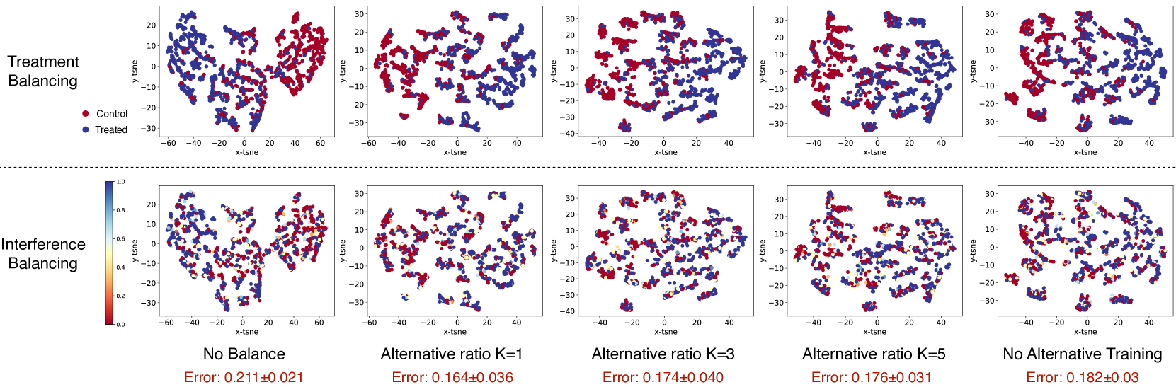
Figure 6. The T-SNE visualization of latent representations under different alternative training settings. Each point represents a unit’s latent representation. The top line is colored by the observed treatments and the bottom line is colored by observed interference. Five columns from left to right: 1) only trained on $L^{\langle Y\rangle}$ (no balancing); 2) $\frac{Iter_{L}}{Iter_{L^{\langle Y\rangle}}}=1$; 3) $\frac{Iter_{L}}{Iter_{L^{\langle Y\rangle}}}=3$; 4) $\frac{Iter_{L}}{Iter_{L^{\langle Y\rangle}}}=5$; 5) only trained on $L$ (no alternative training). Each setting’s corresponding counterfactual estimation error is marked in red.

5.7. How Does Alternative Training Affect CF-GODE?

CF-GODE uses an alternative training strategy to trade off the latent representation balancing and potential outcome prediction. We examine how this trade-off is performed under varying alternative ratios $K$, where $K=\frac{Iter_{L}}{Iter_{L^{\langle Y\rangle}}}$ represents the alternating training between the overall loss $L$ and the outcome prediction loss $L^{\langle Y\rangle}$. Fig. 6 shows the 2-D T-SNE projections of latent representations and their corresponding counterfactual estimation errors for different K values. We note that compared to solely training on $L^{\langle Y\rangle}$ (i.e., no balancing), training with $L$ is able to force the embeddings more balanced, suggesting the effectiveness of our proposed domain adversarial learning based balancing objectives. In addition, with a smaller $K$, CF-GODE achieves better estimation errors, while a bigger $K$ leads to more balanced latent representations. These results confirm that our alternative training is able to trade off between latent representation balancing and potential outcome prediction. In practice, choosing an appropriate value of $K$ is expected to be determined through empirical analysis for each dataset.

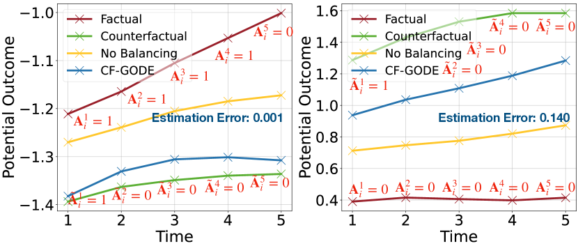
Figure 7. The predicted counterfactual outcomes of CF-GODE w/w.o balancing loss functions. The treatments of factual outcomes $\mathbf{A}_{i}^{t}$ and treatments of counterfactual outcomes $\mathbf{\tilde{A}}_{i}^{t}$ are attached around the corresponding curves at each timestamp. The estimation errors are noted in blue. Results are from Flickr dataset. Left: a successful case; right: a bad case.

5.8. Case Study: When CF-GODE Is Good, and When It Is Not.

To intuitively understand how CF-GODE works in estimating counterfactual outcomes and to study when CF-GODE would fail, we sample one successful unit and one failure unit from Flickr dataset. We draw their factual outcomes, counterfactual outcomes, and the estimations made by CF-GODE and CF-GODE-N (without balancing) in Fig. 7. In the successful case, the estimate by CF-GODE is able to conform to the counterfactual treatment trajectory, while CF-GODE-N still follows the factual trajectory. This shows the effectiveness of our proposed balancing objectives. However, CF-GODE also makes mistakes. In the failure case, its estimate fails to catch up with the counterfactual outcome trajectory, yielding a non-trivial error. We speculate that this is because the counterfactual outcome of this unit is quite distinct from the factual one in terms of data scale, making counterfactual estimation more difficult.

5.9. How Hyperparamters Affect CF-GODE?

The two balancing objectives are core to making CF-GODE causal. Therefore, we finally study the impact of their degrees, represented by $\alpha_{\mathbf{A}}$ and $\alpha_{\mathbf{G}}$ in the loss function, on the model performance. We test $\alpha_{\mathbf{A}}$ and $\alpha_{\mathbf{G}}$ values evenly ranging from $[0,0,1.0]$, and present the counterfactual outcomes estimation errors for each combination of $\alpha_{\mathbf{A}}$ and $\alpha_{\mathbf{G}}$ in Fig. 8. Our results show that the errors are relatively higher when both $\alpha_{\mathbf{A}}$ and $\alpha_{\mathbf{G}}$ are in low values, i.e., light balancing. On the other hand, with larger values, the estimation errors generally become lower, but with high variance. This indicates the effectiveness of the balancing objectives but also highlights the instability of domain adversarial learning based balancing.

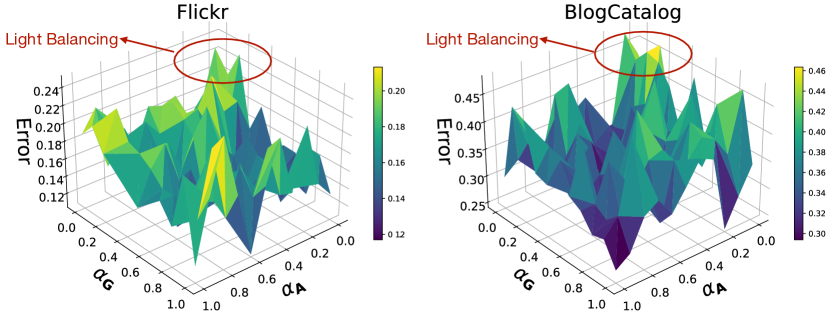
Figure 8. The counterfactual estimation errors w.r.t. different combinations of $\alpha_{\mathbf{A}}$ and $\alpha_{\mathbf{G}}$. The “Light Balancing” settings where $\alpha_{\mathbf{A}}$ and $\alpha_{\mathbf{G}}$ are both in small values are circles in red.

6. Conclusion

In this paper, we study continuous-time counterfactual outcomes estimation in multi-agent dynamical systems, where units interact with each other. To this end, we propose CF-GODE, a novel causal model based on GraphODE to enable continuous potential outcomes prediction, and domain adversarial learning to remove confounding bias. We provide both theoretical justification and empirical analyses to demonstrate the effectiveness of our model. One limitation of CF-GODE is it needs the assumption of strong ignorability for multi-agent dynamical systems, which is not testable in practice. Recent studies relax this assumption by inferring latent proxy variables (Wang and Blei, 2019), which could be a potential solution.

Appendix A Appendix

A.1. Proofs of Theorems

A.1.1. Proof of Theorem. 1

Theorem 1.

Let $j\in\{0,1\}$ be the binary treatment values, and let $N$ and $T$ denote the number of units and observed timestamp lengths, respectively. Let $P_{j}^{t}=P(\mathbf{Z}^{t}\mid\mathbf{A}^{t}=j)$, be the distribution of latent representation $\mathbf{Z}^{t}$ for the group of units with treatments $j$ at time $t$. Let $f$, $\phi$, $d_{\mathbf{A}}^{j}$ be the initial state encoder, the ODE function of treatment-induced GraphODE, and logits of predicting treatment $j$. The necessary and sufficient condition for the min-max game in Eq. (7) to be optimal is $P_{0}^{t}=P_{1}^{t},\forall t\in\left(t_{0},t_{1}\cdots t_{T}\right)$.

The proof of Theorem 1 follows (Bica et al., 2020; Melnychuk et al., 2022) and consists of two steps: to find the optimal $d_{\mathbf{A}}^{j}$ while fixing $f$ and $\phi$, and then to prove the optimal $f$ and $\phi$ while fixing $d_{\mathbf{A}}^{j}$ can balance the latent representations, i.e., $P_{0}^{t}=P_{1}^{t}$. The first step is given by Proposition 1.

Proposition 0.

(Proposition 1 in (Melnychuk et al., 2022)) Let $\alpha_{j}=P(A^{t}=j)$. When the initial state encoder $f$ and ODE function $\phi$ are fixed, the optimal $d_{\mathbf{A}}^{j}$ at time $t$ is:

(10) $${d_{\mathbf{A}}^{j}}^{*}=\frac{\alpha_{j}P_{j}^{t}}{\sum_{j^{\prime}\in\{0,1\}}\alpha_{j^{\prime}}P_{j^{\prime}}^{t}}.$$

Proof.

When fixing $f$ and $\phi$, ${d_{\mathbf{A}}^{j}}^{*}$ is obtained by:

(11) $${d_{\mathbf{A}}^{j}}^{*} =\underset{d_{\mathbf{A}}^{j}}{\text{argmin}}\sum_{j\in\{0,1\}}\mathds{1}_{(\mathbf{A}^{t}=j)}-\log\left(d_{\mathbf{A}}^{j}\left(r(\mathbf{Z}^{t})\right)\right),$$

(12) $$\qquad\qquad\text{subject to }\sum_{j\in\{0,1\}}d_{\mathbf{A}}^{j}\left(r(\mathbf{Z}^{t})\right)=1,$$

where Eq. (11) is adapted from Eq. (7). Note Eq. (11) can be applied to any $i$ and $t$ in Eq. (7), so we disregard the expectation with respect to them. Let $\alpha_{j}=P(A^{t}=j)$ and $P_{j}^{t}=P(\mathbf{Z}^{t}\mid\mathbf{A}^{t}=j)$. Then Eq. (11) can be rewritten as:

(13) $${d_{\mathbf{A}}^{j}}^{*} =\underset{d_{\mathbf{A}}^{j}}{\text{argmin}}\sum_{j\in\{0,1\}}-\mathbb{E}_{\mathbf{Z}^{t}\sim P_{j}^{t}}\alpha_{j}\log\left(d_{\mathbf{A}}^{j}\left(r(\mathbf{Z}^{t})\right)\right)$$

(14) $$=\underset{d_{\mathbf{A}}^{j}}{\text{argmin}}\sum_{j\in\{0,1\}}-\int_{\mathbf{Z^{\prime}}^{t}}\alpha_{j}\log\left(d_{\mathbf{A}}^{j}\left(r({\mathbf{Z^{\prime}}^{t}})\right)\right)P_{j}^{t}d\mathbf{Z^{\prime}}^{t}.$$

We can also take pointwise optimization for any $\mathbf{Z^{\prime}}^{t}$ in Eq. (14) Then by combining Equation (14) with the constraint in Equation (12) and using Lagrange multipliers, we have:

$${d_{\mathbf{A}}^{j}}^{*} =\underset{d_{\mathbf{A}}^{j}}{\text{argmin}}\sum_{j\in\{0,1\}}-\alpha_{j}\log\left(d_{\mathbf{A}}^{j}\left(r({\mathbf{Z^{\prime}}^{t}})\right)\right)P_{j}^{t}$$

(15) $$+\lambda\left(\sum_{j\in\{0,1\}}d_{\mathbf{A}}^{j}\left(r(\mathbf{Z}^{t})\right)-1\right).$$

Let $J=\sum_{j\in\{0,1\}}-\alpha_{j}\log(d_{\mathbf{A}}^{j}(r({\mathbf{Z^{\prime}}^{t}})))P_{j}^{t}+\lambda(\sum_{j\in\{0,1\}}d_{\mathbf{A}}^{j}(r(\mathbf{Z}^{t}))-1)$ be the objective in Eq. (15) The optimal values can be obtained by taking partial gradients $\frac{\partial J}{\partial d_{\mathbf{A}}^{j}}=0$ and $\frac{\partial J}{\lambda}=0$, respectively. By computing them jointly we can obtain ${d_{\mathbf{A}}^{j}}^{*}=\frac{\alpha_{j}P_{j}^{t}}{\sum_{j^{\prime}\in\{0,1\}}\alpha_{j^{\prime}}P_{j^{\prime}}^{t}}$. ∎

The second step is to prove Theorem. 1 that the optimal $f$ and $\phi$ can obtain balanced representations with respect to treatments.

Proof.

With Proposition 1, we can fix the optimal ${d_{\mathbf{A}}^{j}}^{*}$ and find the condition where Eq. (7) achieves optimum. Putting ${d_{\mathbf{A}}^{j}}^{*}$ into the objective in Eq. (7) and applying similar simplifications as in Eq. (14) and Eq. (15), we have:

(16) $$f^{*},\phi^{*} =\underset{f,\phi}{\text{argmax}}\sum_{j\in\{0,1\}}-\mathbb{E}_{\mathbf{Z}^{t}\sim P_{j}^{t}}\log\left(\frac{\alpha_{j}P_{j}^{t}}{\sum_{j^{\prime}\in\{0,1\}}\alpha_{j^{\prime}}P_{j^{\prime}}^{t}}\right)$$

(17) $$=\underset{f,\phi}{\text{argmin}}\sum_{j\in\{0,1\}}\mathbb{E}_{\mathbf{Z}^{t}\sim P_{j}^{t}}\log\left(\frac{P_{j}^{t}}{\sum_{j^{\prime}\in\{0,1\}}\alpha_{j^{\prime}}P_{j^{\prime}}^{t}}\right)+\log(\alpha_{j})$$

(18) $$=\underset{f,\phi}{\text{argmin}}\sum_{j\in\{0,1\}}\text{KL}\left(P_{j}^{t}\Bigg{|}\Bigg{|}{\sum_{j^{\prime}\in\{0,1\}}\alpha_{j^{\prime}}P_{j^{\prime}}^{t}}\right)+\log(\alpha_{j}),$$

where $\text{KL}(\cdot||\cdot)$ is the KL divergence. Note that $\sum_{j\in\{0,1\}}\log(\alpha_{j})$ is constant in observation data. $\text{KL}(\cdot||\cdot)\geq 0$ and it reaches $0$ when the two operands are equal. Therefore, to have $f^{*},\phi^{*}$, for $j\in\{0,1\}$, we have $P_{0}^{t}=P_{1}^{t}={\sum_{j^{\prime}\in\{0,1\}}\alpha_{j^{\prime}}P_{j^{\prime}}^{t}}$. Therefore, the optimal $f^{*},\phi^{*}$ are those who achieve $P_{0}^{t}=P_{1}^{t}$. We can apply this to all the $N$ units and all the $T$ observed timestamps to obtain the global optimum of Eq. (7), which concludes the proof of Theorem 1. ∎

A.1.2. Proof of Theorem 2

Theorem 2.

Let $f$, $\phi$, $d_{\mathbf{G}}$ be the initial state encoder, the ODE function of treatment-induced GraphODE, and the interference predictor. The necessary and sufficient condition for min-max game in Eq. (8) to be optimal is $P(\mathbf{Z}^{t},\mathbf{A}^{t}|\mathbf{G}^{t}=g^{\prime})$ is identical for any $g^{\prime}$.

The proof of Theorem 2 follows (Wang et al., 2020). Similar to Theorem 1’s proof, it first finds the optimum of $d_{\mathbf{G}}$, and then proves that the optimal $f$ and $\phi$ can balance the representations with respect to interference. We first restate the Lemma 4.1 in (Wang et al., 2020) in Proposition. 2.

Proposition 0.

(Lemma 4.1 in (Wang et al., 2020)) Let $\mathbf{C}^{t}=[\mathbf{Z}^{t},\mathbf{A}^{t}]$ be the concatenation of $\mathbf{Z}^{t}$ and $\mathbf{A}^{t}$. When fixing initial state encoder $f$ and ODE function $\phi$, the optimal $d_{\mathbf{G}}$ at time $t$ is:

(20) $$d_{\mathbf{G}}^{*}=\mathbb{E}_{\mathbf{G}^{t}\sim p(\mathbf{G}^{t}|\mathbf{C}^{t})}(\mathbf{G}^{t}).$$

Proof.

Eq. (20) is adapted from Eq. (8). We disregard the expectation with respect to $i$ and $t$ since Eq. (20) is applicable to any $i$ and $t$. If fixing $f$ and $\phi$, the optimal $d_{\mathbf{G}}^{*}$ is given by:

(21) $$d_{\mathbf{G}}^{*} =\underset{d_{\mathbf{G}}}{\text{argmin}}\ \mathbb{E}_{(\mathbf{Z}^{t},\mathbf{A}^{t},\mathbf{G}^{t})\sim p(\mathbf{Z}^{t},\mathbf{A}^{t},\mathbf{G}^{t})}\left(d_{\mathbf{G}}\left(r([\mathbf{Z}^{t},\mathbf{A}^{t}])\right)-\mathbf{G}^{t}\right)^{2}$$

(22) $$=\underset{d_{\mathbf{G}}}{\text{argmin}}\ \mathbb{E}_{(\mathbf{C}^{t},\mathbf{G}^{t})\sim p(\mathbf{C}^{t},\mathbf{G}^{t})}\left(d_{\mathbf{G}}\left(r(\mathbf{C}^{t})\right)-\mathbf{G}^{t}\right)^{2}$$

(23) $$=\underset{d_{\mathbf{G}}}{\text{argmin}}\ \mathbb{E}_{\mathbf{C}^{t}\sim p(\mathbf{C}^{t})}\mathbb{E}_{\mathbf{G}^{t}\sim p(\mathbf{G}^{t}\mid\mathbf{C}^{t})}\left(d_{\mathbf{G}}\left(r(\mathbf{C}^{t})\right)-\mathbf{G}^{t}\right)^{2}.$$

As the quadratic expansion in (Wang et al., 2020), the optimal interference predictor is $d_{\mathbf{G}}^{*}=\mathbb{E}_{\mathbf{G}^{t}\sim p(\mathbf{G}^{t}\mid\mathbf{C}^{t})}(\mathbf{G}^{t})$. ∎

Here we introduce and reformulate Theorem 4.1 in (Wang et al., 2020) as Lemma. 3.

Lemma 0.

(Theorem 4.1 in (Wang et al., 2020)) Given $\mathbb{E}_{x}\mathbb{V}(y\mid x)$ where $\mathbb{V}$ denotes variance, its global optimum can be achieved if and only if for any $x$, $\mathbb{E}(y\mid x)=\mathbb{E}(y)$.

With Proposition. 2 and Lemma. 3, we can prove Theorem. 2.

Proof.

Fixing the optimal $d_{\mathbf{G}}^{*}$ in Proposition. 2, the optimal $f$ and $\phi$ for objective Eq. (23) is:

(24) $$f^{*},\phi^{*} =\underset{f,\phi}{\text{argmax}}\ \mathbb{E}_{\mathbf{C}^{t}\sim p(\mathbf{C}^{t})}\mathbb{E}_{\mathbf{G}^{t}\sim p(\mathbf{G}^{t}\mid\mathbf{C}^{t})}\left(\mathbb{E}_{\mathbf{G}^{t}\sim p(\mathbf{G}^{t}|\mathbf{C}^{t})}(\mathbf{G}^{t})-\mathbf{G}^{t}\right)^{2}$$

(25) $$=\underset{f,\phi}{\text{argmax}}\ \mathbb{E}_{\mathbf{C}^{t}\sim p(\mathbf{C}^{t})}\mathbb{V}\left(\mathbf{G}^{t}\mid\mathbf{C}^{t}\right).$$

Eq. (25) has the same form as the equation in Lemma. 3. Then substituting $x=\mathbf{C}^{t}$ and $y=\mathbf{G}^{t}$ in Lemma. 3, we have $\mathbb{E}(\mathbf{G}^{t}\mid\mathbf{C}^{t})=\mathbb{E}(\mathbf{G}^{t})$. In other words, $\mathbf{G}^{t}\perp\!\!\!\!\perp\mathbf{C}^{t}$. Therefore, we can also use the inverse form that $\mathbb{E}(\mathbf{C}^{t})=\mathbb{E}(\mathbf{C}^{t}\mid\mathbf{G}^{t})=\mathbb{E}([\mathbf{Z}^{t},\mathbf{A}^{t}]\mid\mathbf{G}^{t})$ for any $\mathbf{G}^{t}$, which concludes the proof of Theorem. 2. ∎

A.2. Pseudo-Code of CF-GODE Training

The pseudo-code for training CF-GODE is shown in Algorithm. 1. Specifically, we use an alternative training trick to trade-off the outcome prediction and adversarial balancing.

Algorithm 1 The optimization process of CF-GODE

Input: Multi-agaent dynamical system ${\mathcal{G}}$; the observational data $\left(\left(\mathbf{X}^{t},\mathbf{A}^{t},\mathbf{Y}^{t}\right)\cup\mathbf{V}\right)$; observed timestamps $\left(t_{0},t_{1}\cdots t_{T}\right)$.

Output: Trained initial state encoder $f(\cdot)$; treatment-induced GraphODE function $\phi(\cdot)$; outcome decoder $d_{\mathbf{Y}}(\cdot)$; treatment predictor $d_{\mathbf{A}}(\cdot)$; interference predictor $d_{\mathbf{G}}(\cdot)$.

Training:

Initialize $f(\cdot)$, $\phi(\cdot)$, $d_{\mathbf{Y}}(\cdot)$, $d_{\mathbf{A}}(\cdot)$, $d_{\mathbf{G}}(\cdot)$;

for w = 1, 2, …, W  do $\triangleright$ Train W iterations

     if w%(K+1) = 0 then $\triangleright$ Train with $L^{\langle Y\rangle}$ for 1 steps

         Compute $L^{\langle Y\rangle}$;

         One step optimization for $f(\cdot)$, $\phi(\cdot)$, and $d_{\mathbf{Y}}(\cdot)$:

         $\theta_{f}^{(w+1)}=\theta_{f}^{(w)}-\eta\nabla_{\theta_{f}}L^{\langle Y\rangle}$; $\triangleright$ $\eta$ is learning rate

         $\theta_{\phi}^{(w+1)}=\theta_{\phi}^{(w)}-\eta\nabla_{\theta_{\phi}}L{\langle Y\rangle}$;

         $\theta_{d_{\mathbf{Y}}}^{(w+1)}=\theta_{d_{\mathbf{Y}}}^{(w)}-\eta\nabla_{\theta_{d_{\mathbf{Y}}}}L^{\langle Y\rangle}$;

     else$\triangleright$ Train with $L$ for $K$ steps

         Compute $L$;

         One step optimization for $f(\cdot)$, $\phi(\cdot)$, $d_{\mathbf{Y}}(\cdot)$, $d_{\mathbf{A}}(\cdot)$, $d_{\mathbf{G}}(\cdot)$:

         $\theta_{d_{\mathbf{A}}}^{(w+1)}=\theta_{d_{\mathbf{A}}}^{(w)}-\eta\nabla_{\theta_{d_{\mathbf{A}}}}L$;

         $\theta_{d_{\mathbf{G}}}^{(w+1)}=\theta_{d_{\mathbf{G}}}^{(w)}-\eta\nabla_{\theta_{d_{\mathbf{G}}}}L$;

         $\theta_{d_{\mathbf{Y}}}^{(w+1)}=\theta_{d_{\mathbf{Y}}}^{(w)}-\eta\nabla_{\theta_{d_{\mathbf{Y}}}}L$

         $\theta_{f}^{(w+1)}=\theta_{f}^{(w)}-\eta\nabla_{\theta_{f}}L^{\langle Y\rangle}+\eta\nabla_{\theta_{f}}L^{\langle A\rangle}+\eta\nabla_{\theta_{f}}L^{\langle G\rangle}$;

         $\triangleright$ Gradient reversal

         $\theta_{\phi}^{(w+1)}=\theta_{\phi}^{(w)}-\eta\nabla_{\theta_{\phi}}L^{\langle Y\rangle}+\eta\nabla_{\theta_{\phi}}L^{\langle A\rangle}+\eta\nabla_{\theta_{\phi}}L^{\langle G\rangle}$;

         $\triangleright$ Gradient reversal      

Return $f(\cdot)$, $\phi(\cdot)$, $d_{\mathbf{Y}}(\cdot)$, $d_{\mathbf{A}}(\cdot)$, $d_{\mathbf{G}}(\cdot)$.

A.3. Experimental Settings

Datasets. In observational data, we only have outcomes under one treatment trajectory but not the ground-truths of counterfactual outcomes. Therefore, we follow (Ma et al., 2022; Guo et al., 2020; Veitch et al., 2019) to use semi-synthetic data to evaluate CF-GODE. That is, the graph structure and node features are real, but treatments and potential outcomes are simulated. We use the social networks Flickr and BlogCatalog as in (Guo et al., 2020; Chu et al., 2021; Ma et al., 2021) as the graph $\mathcal{G}$. We follow these works to first encode the node features into low-dimensional embeddings ($10$-dimensional in this paper) via LDA (Blei et al., 2003). We then follow (Jiang and Sun, 2022) to use Metis (Karypis and Kumar, 1998) to split the graph into training/validation/testing sets. To simulate treatment and potential outcomes over time,  (Geng et al., 2017; Bica et al., 2020; Seedat et al., 2022) use a longitudinal simulation environment, which, however, assumes the units are mutually independent. We extend it into our multi-agent dynamical systems setting by considering the neighbor confounders and interference. During the simulation, we are motivated by the vaccine’s use case. Specifically, treatment $\mathbf{A}_{i}^{t}$ denotes getting a vaccine or not at time $t$ of unit $i$. The trajectory of $\mathbf{A}_{i}^{t}$ denotes the vaccine records over time, e.g., a unit may have a booster dose after the initial vaccine. In this case, the time-dependent covariates $\mathbf{X}^{t}$ could be the health condition, static covariates $\mathbf{V}$ could be race or educational background (assuming it does not change during the study) and potential outcome $\mathbf{Y}^{t}$ could be immunity to the virus. As discussed in Sec. 3.1, the potential outcome $\mathbf{Y}^{t}$ is essentially a part of $\mathbf{X}^{t}$. This is a common setting in longitudinal causal inference studies (Bica et al., 2020; Seedat et al., 2022; Melnychuk et al., 2022). During the simulation, we follow this protocol: the health condition $\mathbf{X}^{t}_{i}$ has a value range $[0.1,10]$, in which a higher value means a better health condition. Meanwhile, a higher health condition means a lower probability to receive a vaccine (treatment).

Treatment simulation. The treatment $\mathbf{A}_{i}^{t}$ is affected by a unit’s own time-dependent covariates $\mathbf{X}_{i}^{t}$, static covariates $\mathbf{V}_{i}$ and those of their neighbors. Let $\mathbf{E}_{i}=w_{a}\mathbf{V}_{i}$ denote the effects of static confounders on treatments, where $w_{a}$ is a generated parameter representing this mechanism. The treatment is then simulated by Bernoulli generator with probability the $p_{i}^{t}(a)$ of unit $i$ at time $t$:

$$p_{i}^{t}(a)=\sigma\Biggl{(} \underbrace{\gamma_{a}(\delta_{a}-\bar{\mathbf{X}}_{i}^{t})}_{\text{time-dependent covariates}}+\underbrace{\gamma_{n}\Biggl{(}\delta_{n}-(\frac{1}{|N_{i}|}\sum_{j\in\mathcal{N}_{i}}\bar{\mathbf{X}}_{j}^{t})\Biggr{)}}_{\text{Neighbor time-dependent covariates}}$$

(26) $$+\underbrace{\gamma_{f}\mathbf{E}i}_{\text{Static covariates}}+\underbrace{\gamma_{g}(\frac{1}{|N_{i}|}\sum_{j\in\mathcal{N}_{i}}\mathbf{E}_{j})}_{\text{Neighbor static covariates}}\Biggr{)},$$

where $\sigma(\cdot)$ is sigmoid function. $\gamma_{a}$, $\gamma_{n}$, $\gamma_{f}$ and $\gamma_{g}$ are degrees of time-dependent confounders, neighbor time-dependent confounders, static confounders and neighbor static confounders, respectively. The default values are $[\gamma_{a},\gamma_{n},\gamma_{f},\gamma_{g}]=[10,3.3,10,3.3]$ ($\frac{\gamma_{a}}{\gamma_{n}}=\frac{\gamma_{f}}{\gamma_{g}}=3$), to mimic that a unit’s own confounding factors should affect it more than neighbors. Note $\bar{\mathbf{X}}_{i}^{t}$ is the average time-dependent covariates until $t$. This reflects that past time-dependent covariates also affect the treatment. We set $\delta_{a}=\delta_{n}=5$ as adjustments.

Potential outcome simulation. We follow (Geng et al., 2017; Bica et al., 2020; Seedat et al., 2022) to use a Pharmacokinetic-Pharmacodynamic (PK-PD) model (Goutelle et al., 2008) to simulate the continuous trajectory. PK-PD model is a popular bio-mathematical model and a natural fit for our vaccine use case. As mentioned above, $\mathbf{Y}^{t}$ is essentially a part of $\mathbf{X}^{t}$. Therefore we directly simulate the trajectory of $\mathbf{X}_{i}^{t}$:

$$\frac{d\mathbf{X}^{t}_{i}}{dt}=\mathbf{X}^{t}_{i}\bigg{(} \underbrace{\rho_{u}\log\left(\frac{K}{\mathbf{X}^{t}_{i}}\right)}_{\text{Time-dependt covariates}}+\underbrace{\rho_{n}\log\left(\frac{K}{\mathbf{X}^{t}_{i}}\right)}_{\text{Neighbor time-dependt covariates}}$$

$$+\underbrace{\rho_{f}\mathbf{O}_{i}}_{\text{Static covariates}}+\underbrace{\rho_{g}\sum_{j\in\mathcal{N}_{i}}\mathbf{O}_{j})}_{\text{Neighbor static covariates}}$$

(27) $$+\underbrace{\beta_{a}\mathbf{D}_{i}^{t}}_{\text{Treatment }}+\underbrace{\frac{1}{|N_{i}|}\sum_{j\in\mathcal{N}_{i}}\beta_{n}\mathbf{D}_{j}^{t}}_{\text{Interference}}+\underbrace{e_{i}^{t}}_{\text{Noise }}\bigg{)},$$

where $K$ controls the effects of time-dependent covariates on future potential outcomes. $\mathbf{O}_{i}=w_{x}\mathbf{V}_{i}$ denote the effects of static confounders on potential outcomes, where $w_{x}$ represents this mechanism. $\rho_{u}$, $\rho_{n}$, $\rho_{f}$ and $\rho_{g}$ are degrees of time-dependent covariates, neighbor time-dependent covariates, static covariates and neighbor static covariates, respectively. Their default values are $[\rho_{u},\rho_{n},\rho_{f},\rho_{g}]=[-0.001,-00033,0.001,0.00033]$ ($\frac{\rho_{u}}{\rho_{n}}=\frac{\rho_{f}}{\rho_{g}}=3$). $\beta_{a}$ and $\beta_{n}$ control the strengths of treatment and interference. We set them as $[\beta_{a},\beta_{n}]=[0.03,0.01]$. The values also reflect that a unit’s own covariates and treatment should have stronger effects on its future potential outcomes than neighbors. In reality, the effects of vaccines on providing protection decrease over time. To mimic this phenomenon, we use the following decay function to model the effects of treatments over time as in (Bica et al., 2020; Seedat et al., 2022).

(28) $$\mathbf{D}_{i}^{t}=\tilde{\mathbf{D}}_{i}^{t}+\mathbf{D}_{i}^{(t-1)}/2,$$

where $\mathbf{D}_{i}^{t}$ denote the protection effect at time $t$, and $\tilde{\mathbf{D}}_{i}^{t}$ means a full protection of vaccines given at $t$. In other words, the unit receives a vaccine at time $t$, i.e., $\mathbf{A}_{i}^{t}=1$. We set $\tilde{\mathbf{D}}_{i}^{t}=1$.

A.4. Notation Table

The notations and their corresponding description are in Table. 4.

Table 4. Notations.

Notation	Description
$\mathcal{G}$	Graph that represents multi-agent dynamical system
$\mathcal{V}$	Node set in $\mathcal{G}$
$\mathcal{E}$	Edge set in $\mathcal{G}$
$\mathbf{V}$	Static unit features
$\mathbf{X}^{t}$	Time-dependent covariates at time $t$
$\mathbf{A}^{t}$	Treatment at time $t$
$\mathbf{Y}^{t}$	Observed outcomes at time $t$
$\mathbf{Y}^{t}(A^{t}=a)$	Potential outcomes under treatment $a$
$\mathbf{\bar{X}}^{t}$	Time-dependent covariates collections up to $t$
$\mathbf{\bar{A}}^{t}$	Treatment collections up to $t$
$\mathbf{\bar{Y}}^{t}$	Observed outcomes collections up to $t$
$\mathcal{H}^{t}$	Past observations
$\mathbf{A}^{t}_{\mathcal{N}_{i}}$	Treatments of node $i$’s first-order neighbors
$\mathbf{A}^{t}_{\mathcal{N}_{-i}}$	Treatments of nodes that are
	beyond $i$’s first-order neighbors
$\mathbf{G}_{i}^{t}$	Interference summary variable
$\mathbf{Z}_{i}^{t}$	Continuous latent trajectory for node $i$
$\mathbf{C}_{i}^{t}$	Concatenation of $\mathbf{Z}_{i}^{t}$ and $\mathbf{A}_{i}^{t}$
$g(\cdot)$	Interference summary function
$\phi(\cdot)$	ODE function
$f(\cdot)$	Initial state encoder function
$r(\cdot)$	Gradient reversal layer
$d_{\mathbf{Y}}(\cdot)$	Outcome prediction layer
$d_{\mathbf{A}}(\cdot)$	Treatment prediction layer
$d_{\mathbf{G}}(\cdot)$	Interference prediction layer
$N$	Number of nodes in $\mathcal{V}$
$T$	Number of observed timestamps
$L^{\langle Y\rangle}$	Loss function of outcome prediction
$L^{\langle A\rangle}$	Loss function of treatment prediction
$L^{\langle G\rangle}$	Loss function of interference prediction
$\alpha_{\mathbf{A}}$	Weight of treatment balancing
$\alpha_{\mathbf{G}}$	Weight of interference balancing