Co-design Hardware and Algorithm for Vector Search

Wenqi Jiang¹, Shigang Li¹, Yu Zhu¹, Johannes de Fine Licht¹, Zhenhao He¹, Runbin Shi¹, Cedric Renggli², Shuai Zhang¹, Theodoros Rekatsinas², Torsten Hoefler¹, Gustavo Alonso¹ ¹ETH Zurich ²Apple

(2023)

Abstract.

Vector search has emerged as the foundation for large-scale information retrieval and machine learning systems, with search engines like Google and Bing processing tens of thousands of queries per second on petabyte-scale document datasets by evaluating vector similarities between encoded query texts and web documents. As performance demands for vector search systems surge, accelerated hardware offers a promising solution in the post-Moore’s Law era. We introduce FANNS, an end-to-end and scalable vector search framework on FPGAs. Given a user-provided recall requirement on a dataset and a hardware resource budget, FANNS automatically co-designs hardware and algorithm, subsequently generating the corresponding accelerator. The framework also supports scale-out by incorporating a hardware TCP/IP stack in the accelerator. FANNS attains up to 23.0 $\times$ and 37.2 $\times$ speedup compared to FPGA and CPU baselines, respectively, and demonstrates superior scalability to GPUs, achieving 5.5 $\times$ and 7.6 $\times$ speedup in median and 95^th percentile (P95) latency within an eight-accelerator configuration. The remarkable performance of FANNS lays a robust groundwork for future FPGA integration in data centers and AI supercomputers.

Approximate nearest neighbor search, hardware acceleration, FPGA

^†^†journalyear: 2023^†^†copyright: acmlicensed^†^†conference: The International Conference for High Performance Computing, Networking, Storage and Analysis; November 12–17, 2023; Denver, CO, USA^†^†booktitle: The International Conference for High Performance Computing, Networking, Storage and Analysis (SC ’23), November 12–17, 2023, Denver, CO, USA^†^†price: 15.00^†^†doi: 10.1145/3581784.3607045^†^†isbn: 979-8-4007-0109-2/23/11^†^†ccs: Computer systems organization Parallel architectures^†^†ccs: Information systems Data management systems^†^†ccs: Information systems Information retrieval

1. Introduction

Vector search has emerged as the cornerstone of large-scale information retrieval and machine learning systems. Commercial search engines like Google and Bing process tens of thousands of search queries per second on hundreds of petabytes of data (Bin, [n.d.]; Goo, [n.d.]). These engines employ machine learning models to represent web pages as vectors and retrieve pages by calculating the distances between query vectors and web vectors (Chen et al., 2021; Huang et al., 2020; Xiong et al., 2020; Karpukhin et al., 2020; Khattab and Zaharia, 2020). Recommender systems (Covington et al., 2016; Suchal and Návrat, 2010) also use vector representations for products to identify and recommend items that users may find appealing. Recently, large language models (LLMs) have incorporated vector search to enhance model quality. By inputting relevant documents from a vector database (Guu et al., 2020; Lewis et al., 2020; Borgeaud et al., 2021), LLMs can achieve better performance in various tasks such as open domain question answering and language generation. Vector search is also extensively used in scientific computing, including chemical structure analysis (Bajusz et al., 2015; Willett, 2014) and biomedical data retrieval (Woodbridge et al., 2016; Neumann et al., 2019; Anagnostou et al., 2020).

Refer to caption — Figure 1. FANNS co-designs the hardware and algorithm for vector search. The generated FPGA-based accelerators outperform GPUs significantly in scale-out experiments.

To meet the surging performance demands of vector search systems in the post-Moore’s Law era, designing specialized vector search hardware is a promising direction to explore. Accordingly, we study the hardware specialization of the widely-used IVF-PQ vector search algorithm (Jegou et al., 2010). The algorithm uses an inverted file (IVF) index to group vectors into many vector lists by clustering. It then applies product quantization (PQ) to compress high-dimensional vectors into a series of byte codes, reducing memory consumption and accelerating the similarity evaluation process. When a query arrives, IVF-PQ goes through six search stages to retrieve similar vectors. The main stages include comparing the vector with all the vector list centroids to identify a subset of relevant lists, scanning the quantized vectors within the selected lists, and collecting the topK most similar vectors.

The benefit of hardware-algorithm co-design. Maximizing the performance of an IVF-PQ accelerator is challenging because one needs to carefully balance the design choices of both the hardware and the algorithm. Given a target chip size, there are many valid designs to implement IVF-PQ: how should we choose the appropriate microarchitecture for each of the six IVF-PQ search stages? How should we allocate the limited hardware resources to the six stages? From the algorithm’s perspective, the multiple parameters in IVF-PQ can significantly influence performance bottlenecks and recall. Due to the vast design space, hardware specialization tailored to a specific set of algorithm parameters can achieve better performance-recall trade-offs: as we will show in the experiments, the accelerators without algorithm parameter awareness are 1.3 $\sim$ 23.0 $\times$ slower than the co-designed accelerators given the same recall requirement.

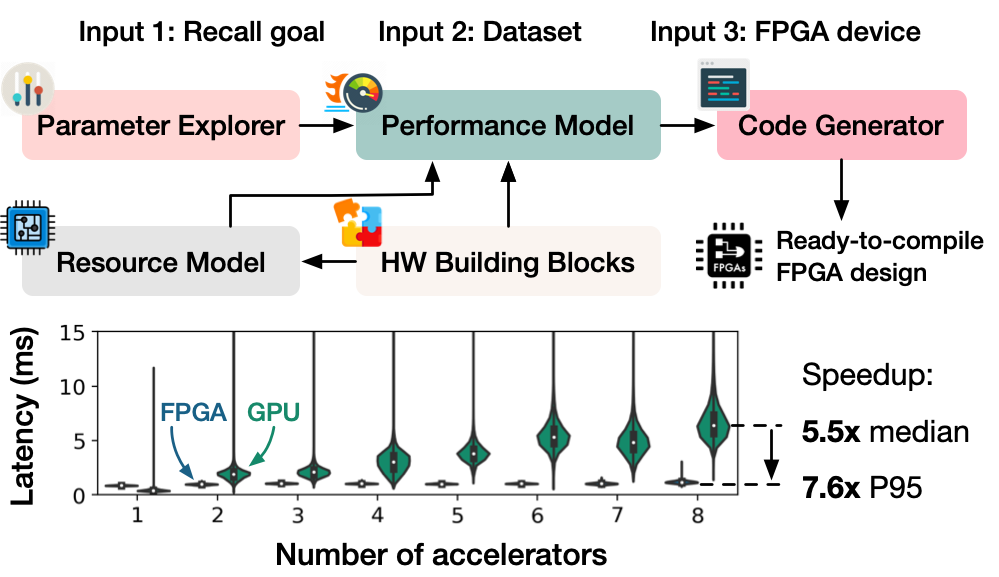
Proposed solution. Considering the numerous design possibilities for an IVF-PQ accelerator, we exploit the reconfigurability of FPGAs to examine various design points. We propose FANNS (FPGA-accelerated Approximate Nearest Neighbor Search), an end-to-end accelerator generation framework for IVF-PQ-based vector search, which automatically co-designs algorithm and hardware to maximize the accelerator performance for target datasets and deployment recall requirements. Figure 1 illustrates the FANNS workflow. Provided with a dataset, a deployment recall requirement, and a target FPGA device, FANNS automatically (a) identifies the optimal combination of parameter settings and hardware design and (b) generates a ready-to-deploy accelerator. Specifically, FANNS first evaluates the relationship between IVF-PQ parameters and recall on the given dataset. It also lists all valid accelerator designs given the FPGA hardware resource budget. Then, the FANNS performance model predicts the queries-per-second (QPS) throughput of all combinations between algorithm parameters and hardware designs. Finally, using the best combination determined by the performance model, the FANNS code generator creates the corresponding FPGA code, which is compiled into an FPGA bitstream. Besides a single-accelerator solution, FANNS can also scale out by instantiating a hardware TCP/IP stack in the accelerator.

Results. Experiments conducted on various datasets demonstrate the effectiveness of the hardware-algorithm co-design: the accelerators generated by FANNS achieve up to 23.0 $\times$ speedup over fixed FPGA designs and up to 37.2 $\times$ speedup compared to a Xeon CPU. While a GPU may outperform an FPGA due to its higher flop/s and bandwidth, FPGAs exhibit superior scalability compared to GPUs thanks to the stable hardware processing pipeline. As shown in Figure 1, experiments on eight accelerators show that the FPGAs achieve 5.5 $\times$ and 7.6 $\times$ speedup over GPUs in median and 95^th percentile (P95) latency, respectively.

Contributions

•

We identify a major challenge in designing accelerators for the IVF-PQ-based vector search algorithm: handling the shifting performance bottlenecks when applying different algorithm parameters.
•

We show the benefit of co-designing hardware and algorithm for optimizing large-scale vector search performance.
•
We propose FANNS, an end-to-end accelerator generation framework for IVF-PQ, maximizing accelerator performance for target datasets and recall requirements. FANNS includes:
- –
  
  A collection of hardware building blocks for IVF-PQ.
- –
  
  An index explorer that captures the relationship between algorithm parameters and recall.
- –
  
  A hardware resource consumption model that returns all accelerator designs on a given FPGA device.
- –
  
  A performance model to predict the accelerator QPS of arbitrary combinations of algorithm parameters and accelerator designs.
- –
  
  A code generator that creates ready-to-compile FPGA code given arbitrary accelerator designs.
•

We demonstrate the impressive performance and scalability of FANNS, achieving 7.6 $\times$ P95 latency speedup over GPUs when utilizing eight accelerators.

2. Background

A vector search takes a query vector $x\in\mathcal{R}^{d}$ as input and retrieves $K$ relevant vector(s) (based on, e.g., L2 distances) from the database $Y$ which contains many $d$ -dimensional vectors. While nearest neighbor search retrieves the exact $K$ closest vectors, really world vector search systems adopt approximate nearest neighbor (ANN) search that trades accuracy for much higher search performance (latency and throughput). The quality of ANN is measured by the recall at $K$ ( $R@K$ ). In this paper, we use the terms vector search and ANN search interchangeably.

2.1. The IVF-PQ Algorithm

We target IVF-PQ because it is one of the most popular algorithms for large-scale ANN (Jegou et al., 2010). Its key elements include (a) partitioning the vectors by the inverted-file index to reduce the percentage of vectors to scan and (b) applying product quantizing to compress the vectors and save memory bandwidth.

Table 1. Definitions of some important symbols.

Symbol	Definition
$x$	A query vector.
$y$	A database vector.
$K$	The number of most similar vectors to return.
$m$	The sub-space number of product quantization.
$nlist$	The totol Voronoi cell number.
$nprobe$	The number of cells to be scanned per query.

2.1.1. Inverted File (IVF) Index

An IVF index partitions a vector dataset $Y$ to many ( $nlist$ ) disjoint subsets by clustering algorithms such as k-means. Each partition is known as a Voronoi cell. At query time, only a few ( $nprobe$ ) Voronoi cells close to the query vector are scanned, such that the scanning workloads are reduced.

2.1.2. Product Quantization (PQ)

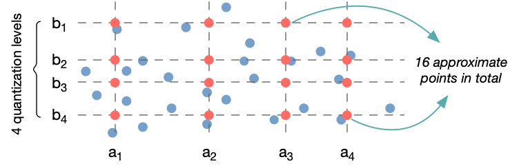
Product quantization (PQ) divides vectors into multiple subvectors and applies quantization per sub-vector space. Figure 2 shows a PQ example on two-dimensional vectors. The example applies four-level quantization per dimension, thus a vector can be approximated by a combination of quantization levels of the two dimensions (e.g., ( $a_{1}$ , $b_{2}$ )).

Practically, PQ can compress a $d$ -dimensional vector to $m$ -byte ( $m<d$ ) PQ codes. Each vector in the dataset is divided into $m$ sub-vectors. Within a sub-vector space, all the sub-vectors are clustered into 256 groups, such that a sub-vector can be approximated by its nearest cluster centroid. As one can represent the cluster ID (0 $\sim$ 255) by one byte, the entire vector can be stored as $m$ -byte PQ codes representing the closest cluster centroids per sub-vector space.

Optionally, one can use optimized product quantization (OPQ) to further improve quantization quality (Ge et al., 2013). The key idea is to rotate the vector space such that the sub-spaces are independent and the variances of each sub-space are normalized. At query time, OPQ simply introduces a vector-matrix multiplication between the query and the transformation matrix, while the rest search procedures are identical to PQ.

2.1.3. The Six Search Stages at Query Time

IVF-PQ contains six search stages for query serving. First, if OPQ is involved, transform the query vector by the OPQ matrix (Stage OPQ). Second, evaluate the distances between a query vector and all Voronoi cell centroids (Stage IVFDist). Third, select a subset of cells that are closest to the query vector to scan (Stage SelCell). Fourth, in order to compare distances between PQ codes and a query vector efficiently, construct a distance lookup table per Voronoi cell (Stage BuildLUT). More specifically, this step divides the query vector into $m$ sub-vectors and computes the distances between the normalized query vector and all centroids of the sub-quantizer. Fifth, approximate the distances between a query vector and the PQ codes (Stage PQDist) by Equation 1, in which $d^{2}(x_{i},\hat{y_{i}}$ only requires looking up the distance tables constructed in Stage BuildLUT. This lookup-based distance computation process is also known as asymmetric distance computation (ADC). Finally, collect the $K$ vectors closest to the query (Stage SelK).

(1)

\hat{d}^{2}(x,y)=d^{2}(x,\hat{y})=\sum_{i=1}^{m}d^{2}(x_{i},\hat{y_{i}})

3. Hardware-Algorithm Design Space

The main challenge in designing compelling IVF-PQ accelerators is to find the optimal option in a huge algorithm-hardware design space, as summarized in Table 2. From the algorithm’s perspective, multiple parameters in IVF-PQ can significantly influence recall and performance bottlenecks. From the hardware’s perspective, there are many valid designs to implement IVF-PQ.

Table 2. The list of choices during design space exploration.

Algorithm parameter space
nlist	The totol Voronoi cell number.
nprobe	The number of cells to be scanned per query.
K	The number of most similar vectors to return.
OPQ_enable	Whether to apply OPQ.
Hardware design space
Design_s	The microarchitecture design of stage $s$ .
#PE_s	The number of processing elements in stage $s$ .
Cache_s	Cache index on-chip or store it off-chip for stage $s\in$ {Stage IVFDist, Stage BuildLUT}.

3.1. Algorithm Parameter Space

To achieve a certain recall requirement, there are many options for selecting algorithm parameters. For example, as we will present in the experiments, all the indexes we evaluated can achieve a target recall of R@100=95% by different nprobe. It is hard to tell which set of parameters we should deploy on the accelerator.

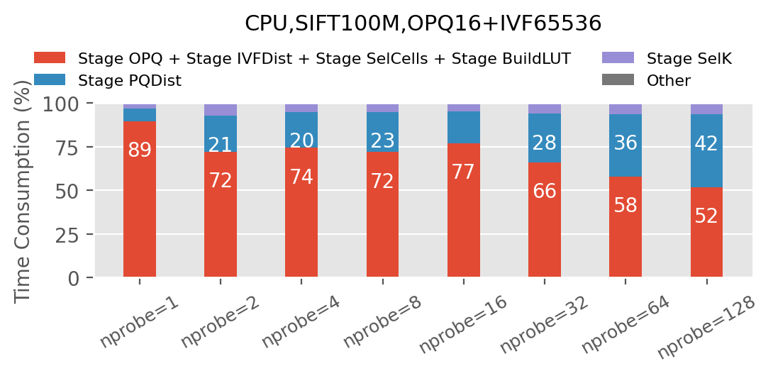
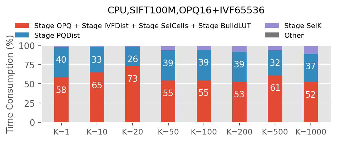
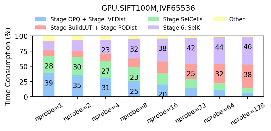
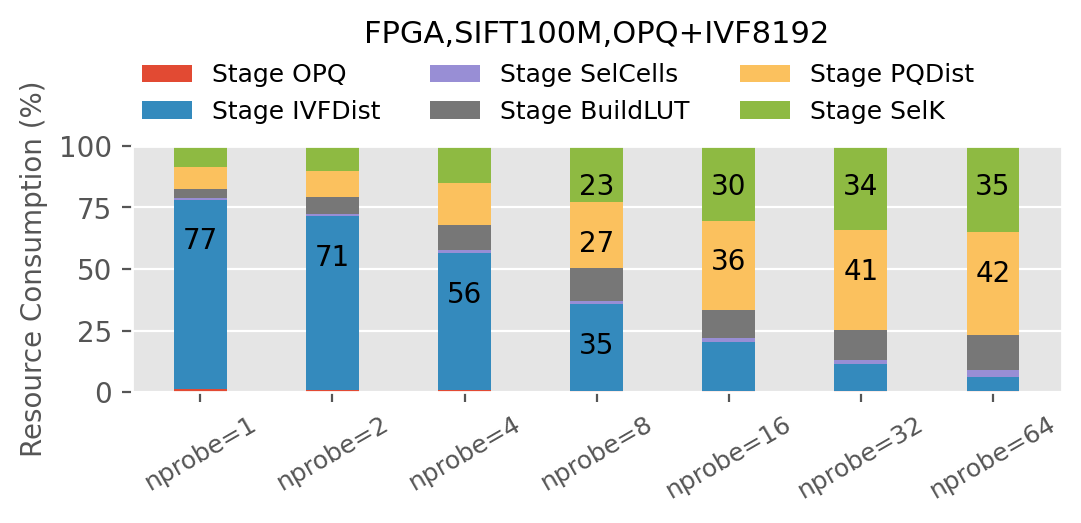
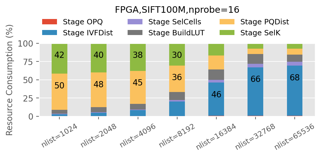
Parameter selections can change the performance bottleneck drastically, which must be considered during the accelerator design phase. We profile the search process on CPUs and GPUs and break down the time consumption per search stage in Figure 3. Unlike many applications with a single outstanding bottleneck, the bottlenecks of IVF-PQ shift between the six search stages when different parameters are used. However, a specialized accelerator cannot handle shifting bottlenecks because it contains a certain number of dedicated processing elements (PE) for each stage. Thus, the accelerator should either target to achieve acceptable performance running arbitrary algorithm parameters or to achieve optimal performance on a certain parameter setting. We now break down the IVF-PQ bottlenecks:

The performance effect of nprobe. We fix the index and tune nprobe. We use the indexes that can achieve the highest QPS of R@100=95% on the SIFT100M dataset on CPU and GPU, respectively. As shown in the first column of Figure 3, increasing the number of cells to scan results in more time consumption in Stage PQDist and Stage SelK, regardless of hardware platforms. The time consumption of these two stages, on GPUs for example, can increase from 20% to 80% as nprobe grows.

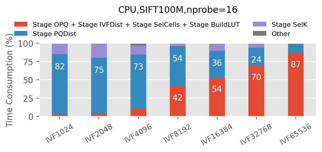
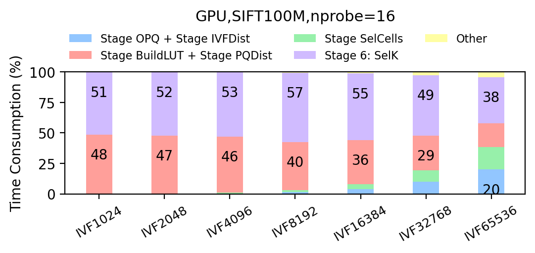
The performance effect of nlist. By contrast to the first experiment, we now observe the effect of the total number of clusters of the index by fixing the number of clusters to scan (nprobe=16). As shown in the second column of Figure 3, higher nlist results in more time consumption on Stage IVFDist to evaluate distances between the query vector and cluster centroids. The consumption is more significant on CPUs due to their limited flop/s compared with GPUs, while the main bottlenecks of GPUs are still in later stages even if nlist is reasonably large.

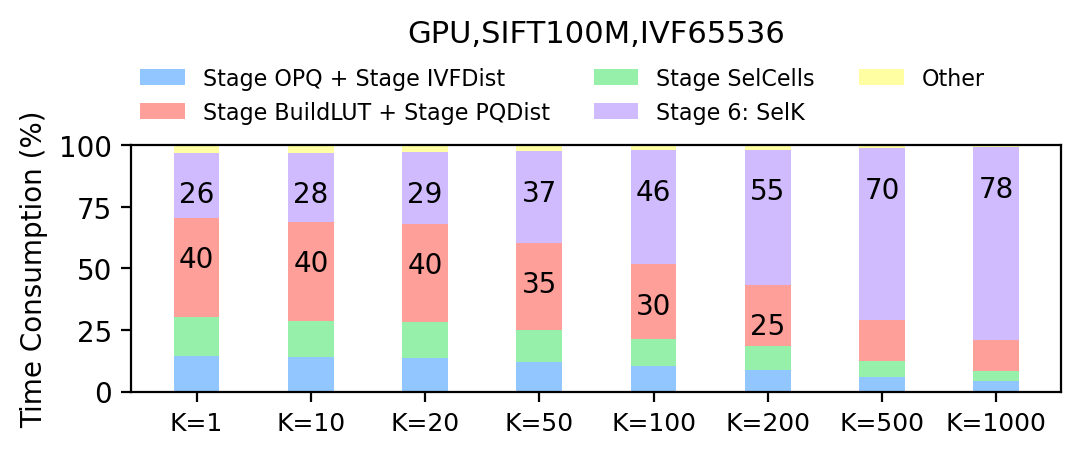
The performance effect of $K$ . We fix the index per hardware as in the $\mathrm{nprobe}$ experiment. As shown in the third column of Figure 3, the time consumption on Stage SelK on GPUs increases significantly as $K$ grows, while the phenomenon is unobvious on CPUs as the bottlenecks are in other stages.

3.2. Hardware Design Space

There are many ways to implement an IVF-PQ accelerator, and the design choices are summarized in Table 2.

The first choice is the microarchitecture per search stage. Not only does the processing element (PE) design differ between stages, there are multiple valid designs per stage. For example, Stage SelK collects $K$ nearest neighbors from a series of distance values, which can either be implemented by a hierarchical priority queue consisting of systolic compare-swap units or by a hybrid design involving sorting network and priority queues, as we will show in Section 5.

The second choice is chip area allocation across the six search stages, i.e., choosing PE numbers per stage. Due to the finite transistors within a chip, this is a zero-sum game: increasing the number of PEs in one stage implies reducing them in another.

The third decision is about index caching. Though storing them in off-chip DRAM is the only option for larger IVF indexes, we can decide whether to cache smaller indexes in on-chip SRAM. Caching index guarantees low accessing latency and high bandwidth but increases hardware resource consumptions.

3.3. How Does One Choice Influence Others?

The choices of algorithm parameters will influence the optimal hardware design and vice versa. Since the relationship between the design choices is intricate, we only convey the intuition here with a couple of examples, while the quantitative model will be presented in later sections. First, tuning a single parameter can affect the optimal accelerator design. Increasing $nlist$ results in more workload in comparing the distances between query vectors and IVF centroids. As a result, more PEs in Stage IVFDist should be instantiated to handle the increasing workload, while fewer PEs can be instantiated in other stages due to the limited chip size. Besides, if the $nlist$ is large enough, caching the IVF index on-chip is not a choice at all, while caching small indexes can be beneficial at the cost of consuming on-chip memory that other PEs could have taken. Second, a specific accelerator design has its favorable parameter settings. Assume the accelerator has a lot of Stage IVFDist PEs, while other stages are naturally allocated with fewer resources. Such design naturally favors a parameter setting of high $nlist$ and low $nprobe$ : the reverse case (low $nlist$ and high $nprobe$ ) will underutilize the Stage IVFDist PEs yet overwhelming the limited Stage PQDist PEs, resulting in low QPS.

3.4. Explore the Design Space by FPGAs

Due to the many design options for an IVF-PQ accelerator as introduced above, we leverage the reconfigurability of FPGAs to show the trade-offs between different designs and to compare performance between these designs.

FPGAs are reprogrammable circuits that consist of BRAM and URAM as fast on-chip memory, Flip-Flops (FF) as registers, and Digital Signal Processors (DSP) as computation units. Various FPGA models have different amounts of those resources. An FPGA-based accelerator usually consists of a number of processing elements (PEs) to implement functionalities and FIFOs to connect the PEs. For example, a neural network accelerator can allocate the computation workload to multiple matrix multiplication PEs and gather the partial results using another PE, and FIFOs enable the streaming communication between these PEs. Developing FPGA accelerators typically requires much more effort than software. Traditionally, FPGAs are developed by hardware description languages (HDL), such as Verilog and VHDL, but recent advances in High-Level Synthesis (HLS) allow programmers to develop the circuit at a higher level using C/C++ or OpenCL (viv, [n.d.]; int, [n.d.]). FPGAs are now widely available in data centers and in the cloud (Jiang et al., 2023).

4. FANNS Framework Overview

We present FANNS (FPGA-accelerated Approximate Nearest Neighbor Search), an end-to-end vector search framework by hardware-algorithm co-design. FANNS targets the deployment scenario where the user (deployer) has a target recall goal (e.g., for all queries, achieve 80% recall for top 10 results on average) on a given dataset and a given hardware device. In this case, FANNS can automatically figure out the optimal combination of algorithm parameters and hardware design, and generate the specialized FPGA accelerator for the combination. FANNS also supports scale-out by instantiating a hardware network stack (He et al., 2021) in the accelerator.

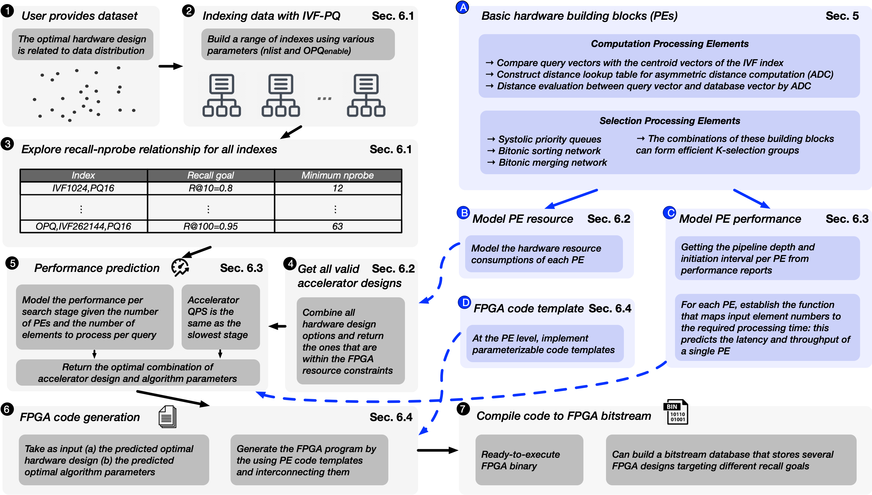
Figure 4 overviews the FANNS workflow.

Framework building blocks ( $\sim$ ). To build an IVF-PQ accelerator, we first build a set of PEs for all six search stages . These building blocks are independent to user requirements. We design multiple PEs per stage when there are several valid microarchitecture solutions. Given the designed PEs, we naturally know their hardware resource consumptions . We can model the PE performance in both latency and throughput : knowing the pipeline depth and initiation interval per PE, one can establish the relationship between the number of input elements to process and the respective time consumption in clock cycles. Finishing the PE design step, we also have a set of PE code templates .

Automatic accelerator generation workflow ( $\sim$ ). The gray blocks in Figure 4 presents the automatic workflow that customizes the hardware per user recall requirement. The inputs of the framework are the user-provided dataset and recall goal . Given the dataset, FANNS trains a number of indexes using a range of parameters . Then, for each index, FANNS evaluates the relationship between nprobe and recall . On the other hand, FANNS returns all valid hardware designs whose resource consumption is under the constraint of the given FPGA device . Subsequently, FANNS uses a performance model to predict the optimal combination of parameter setting and accelerator design . The performance model takes two input sources: (a) the set of all possible accelerator designs by combining different hardware-level options summarized in Table 2 and (b) the minimal nprobe per index given the recall requirement. For each combination of the hardware-level and parameter-level choices, FANNS performance model can predict QPS based on per-PE performance. Given the predicted optimal design, FANNS code generator outputs the ready-to-compile FPGA code by instantiating the respective PEs and interconnecting them . Finally, the FPGA code is compiled to bitstream (FPGA executable) . Table 3 breaks down the time consumption of the FANNS workflow.

Table 3. Time consumption of the FANNS workflow.

Step	Time consumption
Build Indexes	Several hours per index.
Get recall-nprobe relationship	Up to minutes per index.
Predict optimal design	Up to one hour per recall goal.
FPGA code generation	Within seconds.
FPGA bitstream generation	Around ten hours per design.

Framework deployment. Given its ability to optimize accelerator performance based on specific datasets and recall objectives, FANNS is well-suited for integration into production vector search systems. Such systems often manage dynamic datasets, subject to regular insertions and deletions. This is accomplished through the maintenance of a primary IVF-PQ index for a specific dataset snapshot, an incremental (usually graph-based) index for new vectors added since the last snapshot, and a bitmap to track deleted vectors. These two indexes are periodically merged, e.g., once a week, into a new primary index (Wei et al., 2020). In this scenario, FANNS targets optimizing performance for the main index, thus also periodically redesigning accelerators for the new dataset snapshot and, if applicable, the new recall goal. When building the accelerator for the new snapshot, the existing accelerator and the CPU’s incremental index continue to process queries. As such, the time taken to build the new accelerator is effectively concealed by the ongoing operation of the older system, barring the initial build. This setup also allows FANNS to always target a static dataset snapshot. The algorithm explorer, therefore, does not need to handle any shifts in data distribution, allowing accurate performance modeling.

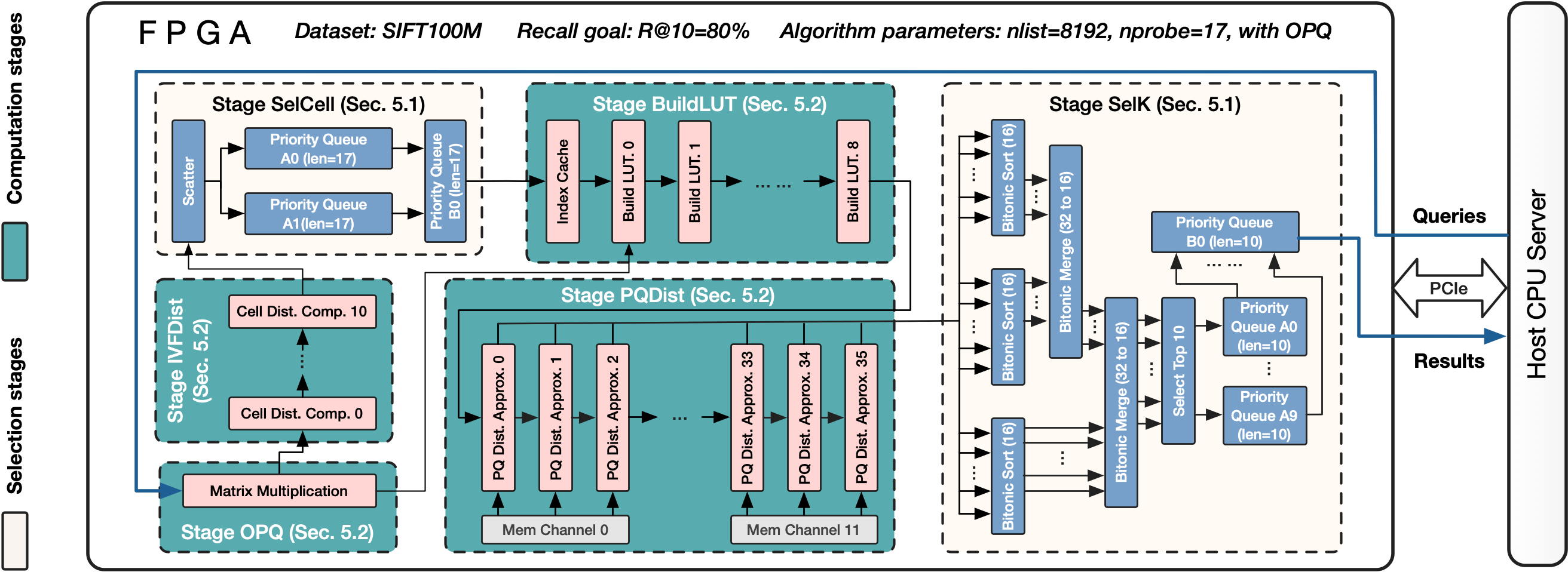
Example FPGA design. Figure 5 shows a generated accelerator targeting R@10=80% on the SIFT100M dataset. In this single-accelerator-search scenario, the FPGA communicates with the host CPU through PCIe to receive query requests and return results. FANNS processes queries in a deeply pipelined fashion: there can be multiple queries on the fly in different stages in order to maximize throughput. Each stage of processing is accomplished by a collection of PEs. The arrows connecting those PEs are FIFOs: a PE loads values from the input FIFO(s), processes the inputs, and pushes the results to the output FIFO(s). A stage can contain homogeneous PEs such as Stage IVFDist or heterogeneous PEs such as Stage SelK which involves sorting networks, merging networks, and priority queues. The PE numbers are typically irregular (11 in Stage IVFDist, 9 in Stage BuildLUT, etc.) as they are calculated by the performance model, unlike being restricted to the exponential of two which human designers favor. We will specify the hardware design per search stage in the following section.

5. Hardware Processing Elements

We present the accelerator hardware processing elements and the design choices. We group the six search stages into selection stages and computation stages to explain related concepts together.

5.1. Designs for the Selection Stages

Two stages need selection functionality. Stage SelCells selects the closest Voronoi cells to the query vector, given a set of input distances. Stage SelK collects the $K$ smallest distances between the query vector and database vectors, given the many approximated distances output by Stage PQDist every clock cycle. Since there can be multiple PEs producing inputs to the two stages, the selection hardware should support multiple input streams.

5.1.1. $K$ -Selection Primitives

Bitonic sort networks and systolic priority queues are the building blocks for $K$ -selection.

Bitonic Sort. Bitonic sort is a parallel sorting algorithm that takes several input elements in parallel, performs a certain series of compare-swap operations, and outputs the sorted array. Bitonic sort exhibits high sorting throughput, and its parallelism aligns very well with FPGAs (Batcher, 1968; Mueller et al., 2012; Papaphilippou et al., 2018; Song et al., 2016; Salamat et al., 2021; Papaphilippou et al., 2020). As a result, the latency of sorting an array is $\sum_{i=1}^{log_{2}l}i=\frac{log_{2}l*(1+log_{2}l)}{2}$ clock cycles where $l$ is the width of the sorting network.

Systolic Priority Queue. While software-based priority queues support enqueue, dequeue, and replace operations, we only need the replace operation: if the input is smaller than the current root, dequeue the root and enqueue the input. Figure 6 shows in the implemented systolic priority queue (Huang et al., 2014; Leiserson, 1979) that supports such minimal required functionality while consuming the least hardware resources. It is a register array interconnected by compare swap units, supporting one replace operation every two clock cycles. In the first cycle, the leftmost node is replaced with a new item, and all the even entries in the array are swapped with the odd entries. In the second cycle, all the odd entries are swapped with the even entries. During this process, the smallest elements are gradually swapped to one side of the queue.

5.1.2. $K$ -Selection Microarchitecture Design

Parallel $K$ -selection collects the $s$ smallest numbers per query ( $s=nprobe$ in Stage SelCells; $s=K$ in Stage SelK) out of $z$ input streams given that each stream produces $v$ values per query. We propose two design options for this task with different trade-offs:

Option 1: hierarchical priority queue (HPQ). We propose HPQ as a straightforward way for parallel selection. The first level of HPQ contains $z$ queues to collect $s$ elements from each stream. The second level takes the $zs$ elements collected in the first level and selects the $s$ results. The HPQ allows $z/2$ input elements per cycle since each replace operation in a priority queue requires two cycles. As a result, if an input stream generates one element per cycle, we should split it into two substreams and match it with two priority queues in the first level.

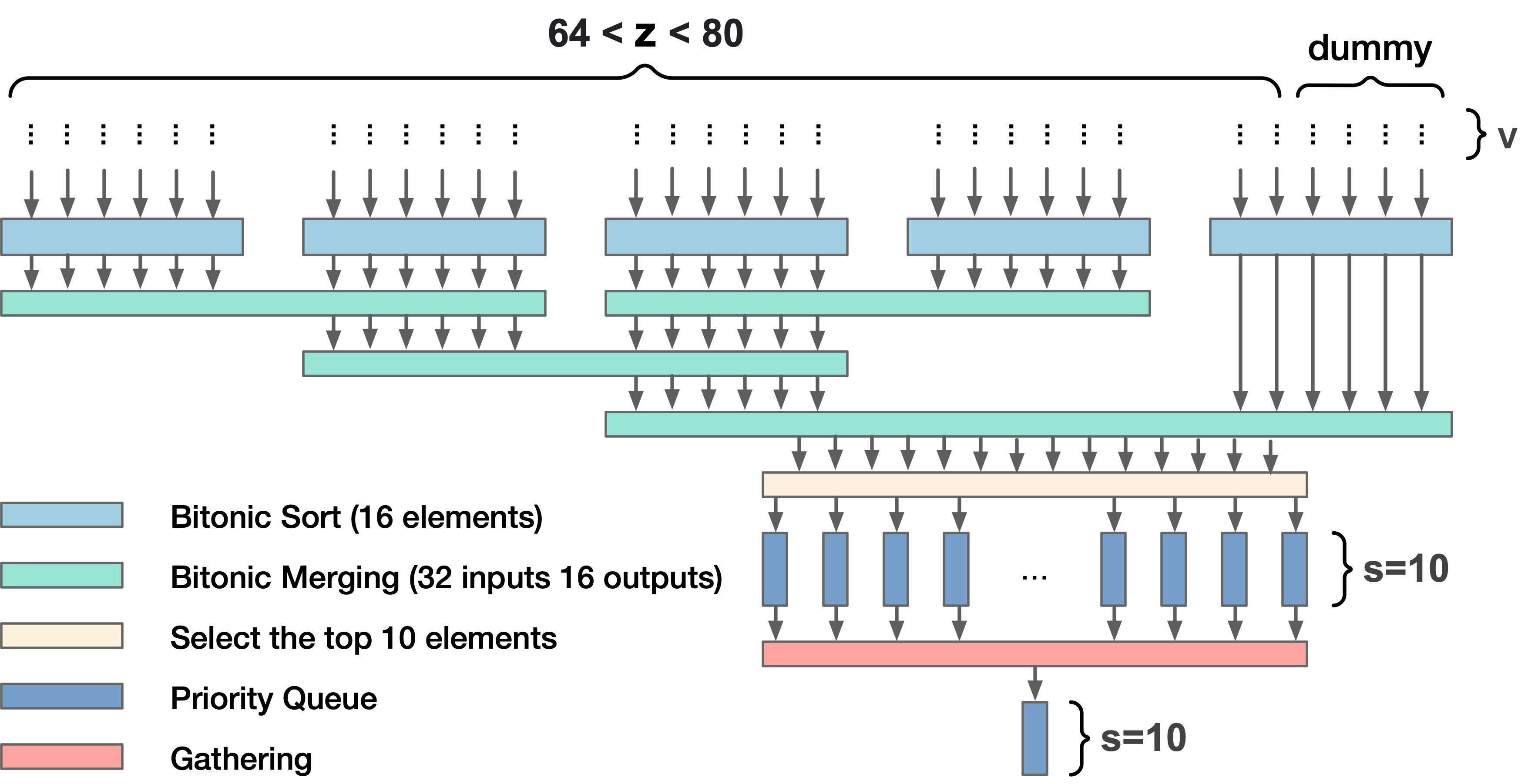
Option 2: hybrid sorting, merging, and priority queue group (HSMPQG). The key idea is to collect the $s$ results per clock cycle before inserting them into the priority queues, such that the number of required queues can be significantly reduced. Figure 7 shows an example of such design ( $64<z\leq 80$ and $s=10$ ). The first step is to sort every 16 elements since 16 is the minimum bitonic sort width greater than $s=10$ . Handling up to 80 inputs per cycle requires five bitonic sort networks. Some dummy streams are added as the input for the last sorting network. The second step is to merge the sorted elements by several bitonic partial mergers. Each bitonic merger outputs the top 16 elements out of the two input sorted arrays. After several merging steps, we have the sorted top 16 elements per cycle. Afterward, the $s=10$ elements per cycle are picked out of the 16 and inserted into a hierarchical priority queue, which outputs the $s$ results per query. Note that we can configure the number of bitonic sort and parallel merge networks for different workloads. For example, if $16<z\leq 32$ , two sorting and one merging modules are required; we will need three sorting and two merging networks when $32<z\leq 48$ .

Intuition behind different $K$ -selection microarchitecture. The HPQ design suits the situation when the input stream number $z$ is small, because the few priority queues instantiated will not consume many resources. This design is also the only option when $s\geq{z}$ , for which the second option cannot filter out unnecessary elements per cycle at all. The HSMPQG design targets to collect a small result set over many input streams. It could save hardware resources by significantly reducing the number of priority queues compared with the first option. However, the bitonic sorting and merging networks also count for resource consumption, thus the second option is not always better even if $s<z$ .

5.2. Designs for the Computation Stages

Computation stages include Stage OPQ, Stage IVFDist, Stage BuildLUT, and Stage PQDist. In this section, we first specify the Stage PQDist PEs to convey the compute PE design principles on FPGAs, and then introduce the PE interconnection topology.

5.2.1. Stage PQDist.

As shown in Figure 5, there are many Stage PQDist PEs working in parallel, approximating distances between the query vector and the quantized database vectors.

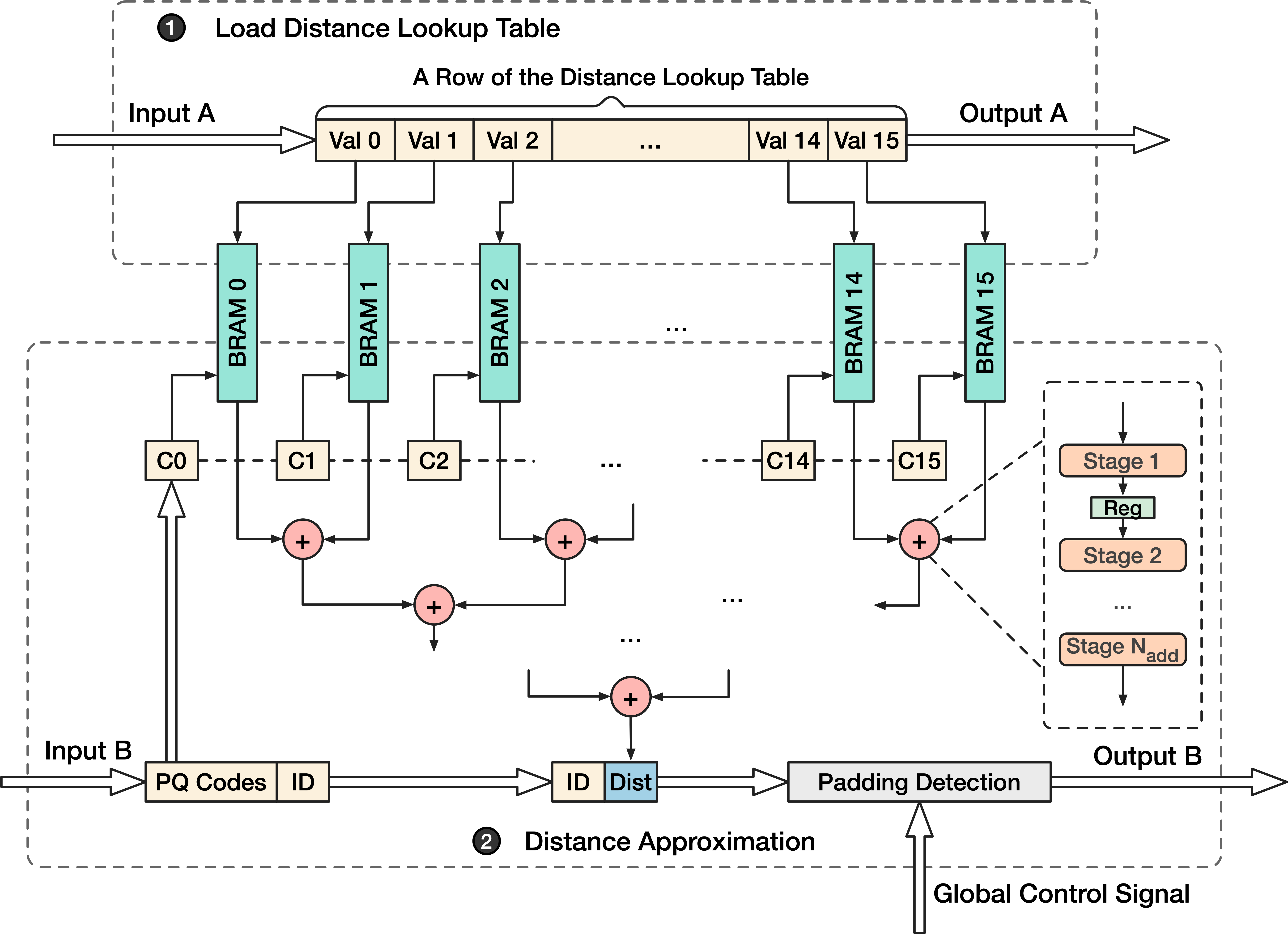
PE design. Figure 8 presents the PE design for decoding 16-byte PQ codes. The PE takes two inputs: the distance lookup tables produced by Stage BuildLUT and the PQ codes stored in off-chip memory channels. For a single query, a PE repeats two major steps $nprobe$ times. The first step is reading a distance lookup table of size of $km$ . We use BRAM, a type of fast on-chip SRAM, to cache the tables. In order to provide memory access concurrency for the computing step, we assign $m$ BRAM slices per PE — each slice stores a column of a table. The second step is approximating the distances between the query vector and the database vectors by asymmetric distance computation. Each PQ code (1-byte) of a database vector is used as the lookup index for one column of a distance table, and $m$ distances are retrieved from the BRAM slices in parallel per cycle. These partial distances are then fed into an add tree that produces the total distance. In order to maximize the computation throughput, each logical operator (addition) in the tree is composed of several DSPs (for computation) and FFs (as registers), such that the computation is fully pipelined, allowing the add tree to consume $m$ input distances and to output one result per clock cycle. During the last iteration of scanning a cell, the PE performs padding detection and overwrites the output by a large distance for the padded case. The meta-info about padding is streamed into the PE by the accelerator’s global controller.

PE size. In principle, a PE with more computation logic is usually more efficient in terms of performance delivered per hardware resource unit. This is because each PE has some surrounding logic as the interface to other PEs — the smaller each PE, the more significant the total overhead. However, it is hard for the FPGA compiler to map a huge chunk of logic to the FPGA successfully (de Fine Licht et al., 2020b). Thus, we experiment with several PE sizes and select the largest one that can be successfully compiled.

5.2.2. PE interconnection Topology.

Within a computation stage, we adopt a 1-D array architecture to forward data between the homogeneous PEs. For example, the second PE consumes the query vector and the results of the first PE, appends its local results, and sends the query vector as well as the aggregated results to the third PE. Another design choice, which we do not adopt, is the broadcasting/gather topology. The advantage of the 1-D array architecture over the broadcasting/gather one is the minimized wire fan-out: too many long wires connected to a single source can lead to placement & routing failure during FPGA compilation (de Fine Licht et al., 2020a). For communication between stages and within a selection stage, the FIFO connections are straightforward because there is no input sharing as in computation stages.

6. End-to-End Hardware Generation

This section illustrates the end-to-end accelerator generation flow of FANNS, as visualized in Figure 4 ( $\sim$ ). We implement the end-to-end generation flow using a set of Python scripts, while the hardware processing elements are implemented in Vitis HLS.

6.1. Explore Algorithm Parameters

Given a dataset, FANNS first captures the relationship between the algorithm parameters and recall, which will be used for accelerator QPS prediction. FANNS trains a number of IVF indexes trying different nlist . Each index is trained both with and without OPQ. Given the user-provided sample query set, FANNS evaluates the minimum nprobe that can achieve the user-specified recall goal on each index (e.g., 80% of average recall for top 10 results). The result of this step is a list of index-nprobe pairs that serve as the inputs of the FPGA performance model.

6.2. List Valid Accelerator Designs

FANNS lists all valid accelerator designs on a given FPGA device by resource consumption modeling . Specifically, FANNS combines all hardware choices in Table 2 to form accelerators and returns the valid ones whose consumptions of all types of resources (BRAM, URAM, LUT, FF, and DSP) are under the device constraint. Consuming all resources on the FPGA is unrealistic because such designs will fail at the placement & routing step during FPGA compilation. But it is also impossible to predict the maximum resource utilization per design because the EDA algorithms for FPGA compilation are nondeterministic. As a result, we set the resource utilization rate as a constant for all accelerators, e.g., a conservative value of 60% in our experiments.

(2)

$\begin{gathered}\sum_{i}C_{r}(PE_{i})+\sum_{i}C_{r}(FIFO_{i})+C_{r}(infra)\leq Constraint_{r},\\ \forall r\in\{BRAM,URAM,LUT,FF,DSP\}\end{gathered}$

FANNS models an accelerator’s resource consumption by summing up several components as in Equation 2 ( $C_{r}$ denotes the consumption of resource $r$ ). The first part is of all the PEs. The consumption of a PE is known once we finish designing and testing the PE. For priority queues of variable lengths, we employ a linear consumption estimation model since the numbers of registers and compare-swap units in a priority queue are linear to the queue length. The second part is the FIFOs connecting PEs, which can be modeled by measuring the consumption of a single FIFO and counting the required FIFO numbers. The final component is the infrastructure surrounding the accelerator kernel, such as the memory controller, which consumes constant resources.

6.3. Model Accelerator Performance

The FANNS performance model predicts the QPS of all combinations of algorithm parameters and accelerator designs, then returns the optimal one. Given the large design space, it is unrealistic to evaluate QPS by compiling all accelerators and testing all parameters. Thus, we need an effective performance model to predict the QPS per combination . By using the following modeling strategy, FANNS can evaluate all (millions of) combinations given a recall requirement within an hour. We now introduce the model in a top-down manner.

Model the performance of an accelerator. As the six search stages of IVF-PQ are pipelined, the throughput of the entire accelerator is that of the slowest stage, as in Equation 3.

(3)

$\begin{gathered}QPS_{accelerator}=min(QPS_{s})\mathrm{,where~{}}s\in\mathrm{\{Stages}\}\end{gathered}$

Model the performance of a search stage. A search stage typically consists of multiple PEs functioning concurrently. If these PEs share the same amount of workload, the time consumption per query of the stage is the same as the time consumption for a single PE to handle its own workload. If the workloads are imbalanced per PE, the performance of the stage is decided by its slowest PE.

Model the performance of a PE. Inspired by de Fine Licht et al. (de Fine Licht et al., 2020a), we estimate the throughput of a single PE by predicting the number of clock cycles it takes to process a query ( $CC$ ). For a single query, we suppose that the PE processes $N$ input elements. The pipeline initiation interval is $II$ , which represents the number of cycles that must pass before a new input can be accepted into the pipeline. The pipeline has a latency $L$ , which is the number of cycles it consumes for an input to propagate through the pipeline and arrive at the exit. $L$ and $II$ are known constants after implementing the hardware. $N$ can be either a constant or a variable. For example, after deciding the algorithm parameters and the accelerator design, the number of distances evaluated per PE in Stage IVFDist is a constant (N=nlist/PENum). By contrast, the number of PQ codes scanned in Stage PQDist differs for every query due to the imbalanced number of codes per cell. In this case, we estimate $N$ by taking the expected scanned entries per query (assume the query vector distribution is identical to the database vectors, such that cells containing more vectors are more likely to be scanned). Given the numbers of $L$ , $II$ and $N$ , we can estimate the consumed clock cycles as $CC=L+(N-1)*II$ . The QPS of the PE can then be derived by Equation 4 where freq is the accelerator frequency. Similar to predicting the maximum resource utilization rate, it is impossible to know the operational frequency of an accelerator before compilation. Thus, we assume the frequency to be a constant for all accelerators.

(4)

\begin{gathered}QPS_{PE}=freq/(L+(N-1)*II)\end{gathered}

6.4. Generate FPGA Programs

FANNS code generator takes as inputs the optimal combination of parameter setting and hardware design and produces the ready-to-compile FPGA code. Refering to the inputs, the code generator instantiates the given numbers of PEs using the PE code templates, the respective on-chip memory for index caching, the FIFOs interconnecting the aforementioned components, and the off-chip memory interfaces between the accelerator kernel and the FPGA shell . Since the code generation step does not involve complex logic, it only consumes seconds to return the FPGA program, which will be further compiled to the bitstream .

7. Evaluation

This section shows the effectiveness and necessity of algorithm-hardware co-design to achieve the optimal vector search performance on FPGAs. We also integrate the FPGAs with network stacks to show their great scalability.

7.1. Experimental Setup

Baseline. We compare FANNS with CPU, GPU, and FPGA baselines. The CPU and GPU baselines run Faiss (version 1.7.0), a popular ANN library developed by Meta known for its efficient IVF-PQ implementation. The FPGA baseline uses the same set of hardware building blocks as FANNS but without being parameter-aware.

Hardware Setup. We choose CPUs, GPUs, and FPGAs that are manufactured in the generation of technology. We use an m5.4xlarge CPU server on AWS, which contains 16 vCPUs of 16 vCPUs of Intel(R) Xeon(R) Platinum 8259CL @ 2.50GHz (Cascade Lake, 14nm technology) and 64 GB of DDR4 memory. We use NVIDIA V100 GPUs (CUDA version 11.3) manufactured by the TSMC 12 nm FFN (FinFET NVIDIA) technology (5,120 CUDA cores; 32 GB HBM). We use Xilinx Alveo U55c FPGA fabricated with TSMC’s 16nm process. It contains 1.3M LUTs, 9K DSPs, 40MB on-chip memory, and 16 GB HBM. We develop the accelerators using Vitis HLS 2022.1.

Benchmark. We evaluate FANNS on standard and representative vector ANN benchmarks: the SIFT and Deep datasets. The SIFT dataset contains 128-dimensional vectors, while the Deep dataset consists of 96-dimensional vectors. For both datasets, we adopt the 100-million-vector size scale as they can fit into the FPGA memory after product quantization. Both datasets contain 10,000 query vectors and respective ground truths of nearest neighbor search for recall evaluation. We set various recall goals on each dataset. As recalls are related to $K$ (the more results returned, the more likely they overlap with true nearest neighbors) and the data distribution, we set one recall goal per K per dataset, i.e., R@1=30%, R@10=80%, and R@100=95% on the SIFT dataset and R@1=30%, R@10=70%, and R@100=95% on the Deep dataset.

Parameters. We explore a range of algorithm parameters and set a couple of constant factors for FANNS performance model. On the algorithm side, we trained a range of indexes with different numbers of Voronoi cells (nlist ranges from $2^{10}$ to $2^{18}$ ) for each dataset, so as to achieve the best QPS for not only FPGA but the CPU and GPU baselines. Per nlist, we trained two indexes with and without OPQ to compare the performance. We quantize the vectors to 16-byte PQ codes ( $m=16$ ) for all indexes and all types of hardware. The primary consideration is to fit the dataset within FPGA’s device memory while achieving high recall. On the FANNS side, we set the maximum FPGA resource utilization rate as 60% to avoid placement & routing failures. We also set the target accelerator frequency as 140MHz based on our design experience with the U55c FPGA device.

7.2. FANNS-Generated Accelerators

This section presents the FANNS generated accelerators. We show that the optimal designs shift with parameter settings. We then present the fully customized accelerator designs under target recall and compare them against the parameter-independent FPGA baseline design.

7.2.1. The Effect of Algorithm Parameters on Hardware Designs

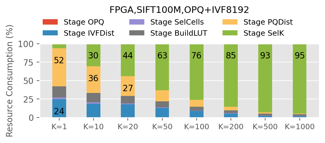
Optimal accelerator designs shift significantly with algorithm parameters, as shown in Figure 9. In this experiment, we assign the parameters to the FANNS performance model, which predicts the optimal hardware design under the parameter constraints. To draw high-level conclusions from the designs, we only visualize the resource consumption ratio per search stage, omitting the microarchitecture-level choices. First, we observe the effect of nprobe on the designs. As the number of PQ codes to scan increases, more hardware resources are dedicated to Stage PQDist and Stage SelK, while most of the resources are allocated to Stage IVFDist when $nprobe$ is small. Then, we fix nprobe and observe the designs when shifting nlist. As nlist raises, more PEs are instantiated for Stage IVFDist so as to improve the performance of centroid distance computation. Finally, as $K$ increases, the resources spent on Stage SelK surge because the resource consumption of hardware priority queues is linear to the queue length $K$ .

7.2.2. The Optimal Accelerator Designs of Given Recall Goals

Table 4 summarizes the FANNS-generated designs per recall and compares them with the baseline designs. It shows that:

First, FANNS picks different parameters per recall. For the three recall requirements, FANNS adopts different indexes and $nprobe$ to maximze the performance.

Second, FANNS generates different hardware designs for each recall requirement. Stage SelK, for example, applies the two different microarchitecture designs (HPQ and HSMPQG) and invests different amounts of hardware resources (2.9% $\sim$ 31.7% LUT) for the three recall requirements. Even for the stages using the same microarchitecture, e.g., Stage IVFDist, the PE numbers of these accelerators can also be different.

7.2.3. Parameter-independent Accelerator Designs

We design a set of parameter-independent ANNS accelerators that can serve queries on arbitrary indexes as the FPGA baseline. We design three parameter-independent accelerators for different $K$ requirements (1, 10, 100) as shown in Table 4. Each accelerator roughly balances resource consumption across stages such that the accelerator should perform well on a wide range of algorithm settings. Saying this, we do not simply allocate 1/6 resources to each of the six stages due to the following facts. First, the number of PEs between Stage PQDist and Stage SelK should be proportional, as more distance computation PEs should be matched with more priority queues to balance the performance between the two stages. Second, Stage OPQ performs a lightweight vector-matrix multiplication that consumes few resources.

Table 4. Comparison between human-crafted design and FANNS-generated designs (for the SIFT100M dataset), including index selection, architectural design, resource consumption (LUT), and predicted QPS.

	Index	nprobe	Stage OPQ		Stage IVFDist			Stage SelCells			Stage BuildLUT			Stage PQDist		Stage SelK			Pred. QPS (140 MHz)
	Index	nprobe	#PE	LUT.(%)	#PE	Index store	LUT.(%)	Arch.	#InStream	LUT.(%)	#PE	Index store	LUT.(%)	#PE	LUT.(%)	Arch.	#InStream	LUT.(%)	Pred. QPS (140 MHz)
K=1 (Baseline)	N/A	N/A	1	0.2	10	HBM	6.9	HPQ	2	6.4	5	HBM	6.9	36	15.2	HPQ	72	1.8	N/A
K=10 (Baseline)	N/A	N/A	1	0.2	10	HBM	6.9	HPQ	2	6.4	4	HBM	6.3	16	6.7	HPQ	32	5.7	N/A
K=100 (Baseline)	N/A	N/A	1	0.2	10	HBM	6.9	HPQ	2	6.4	4	HBM	6.3	4	1.7	HPQ	8	15.0	N/A
K=1 (FANNS)	IVF4096	5	0	0	16	on-chip	11.0	HPQ	2	0.3	5	on-chip	2.6	57	24.0	HPQ	114	2.9	31,876
K=10 (FANNS)	OPQ+IVF8192	17	1	0.2	11	on-chip	7.6	HPQ	2	0.9	9	on-chip	5.2	36	15.2	HSMPQG	36	12.7	11,098
K=100 (FANNS)	OPQ+IVF16384	33	1	0.2	8	on-chip	5.5	HPQ	1	0.6	5	on-chip	3.6	9	3.8	HPQ	18	31.7	3,818

7.3. Performance Comparison

7.3.1. Offline Batch Processing

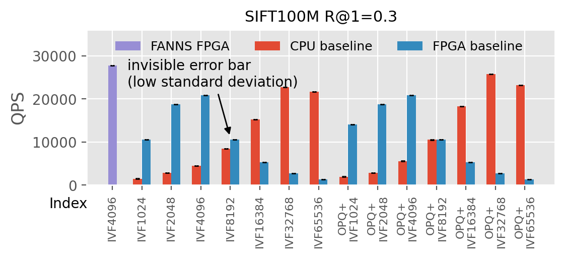
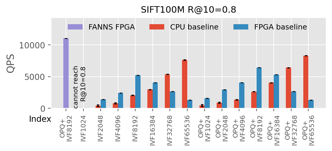
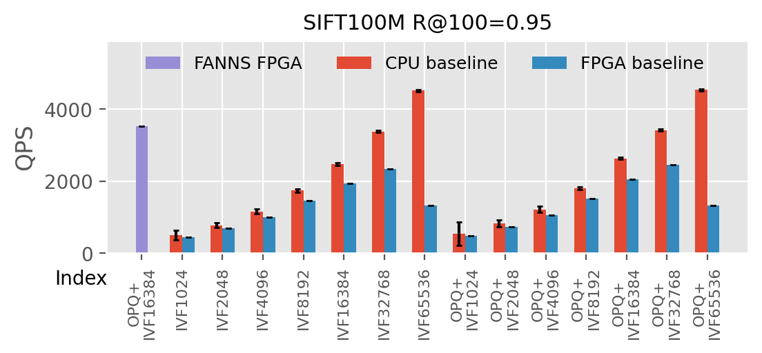
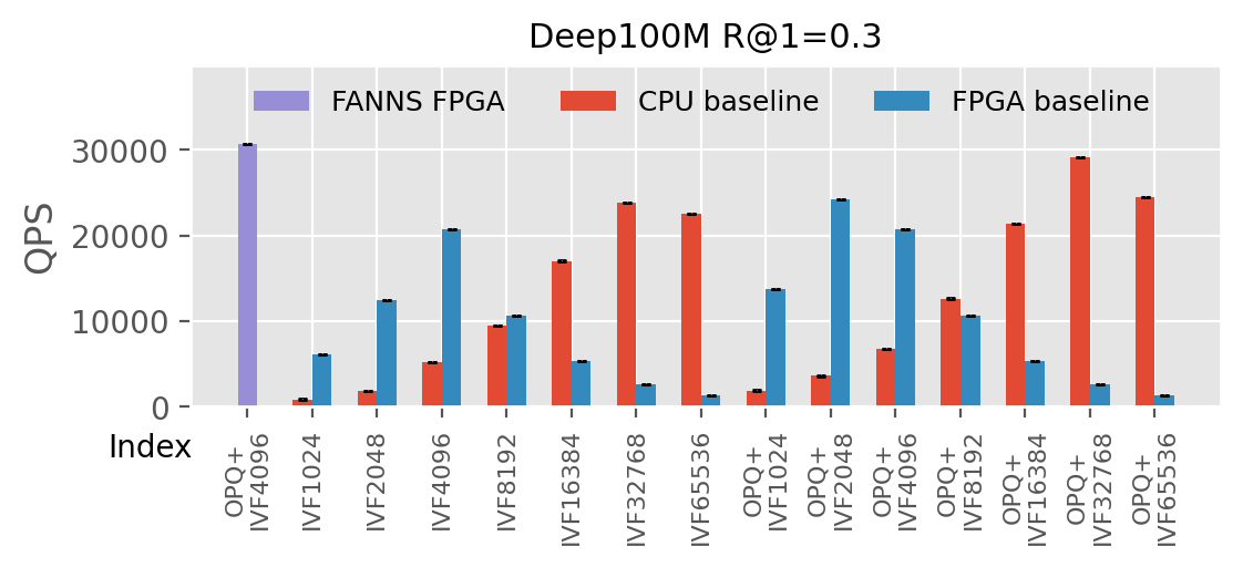
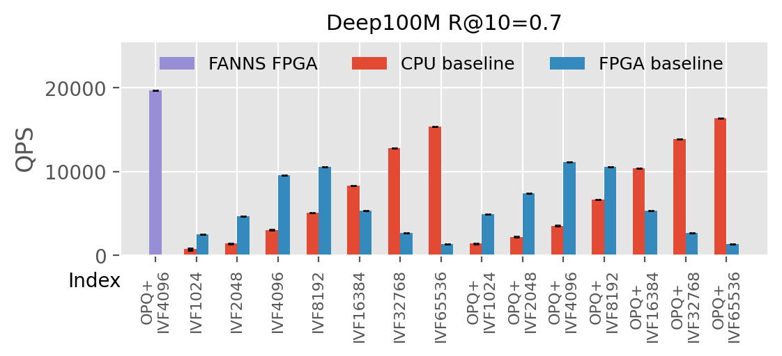
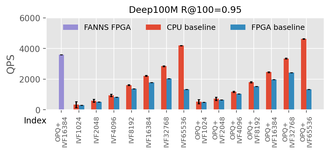
We first compare the throughput (QPS) between FANNS and the CPU/FPGA baselines in Figure 10. The throughput experiments have no latency constraints, thus allowing query batching (size = 10K) to report the highest QPS. FANNS reports $1.3\sim 23.0\times$ QPS as the baseline FPGA designs and $0.8\sim 37.2\times$ as the CPU. As FPGAs have two orders of magnitude lower flop/s than GPUs, GPU still achieves significantly higher QPS than FPGAs ( $5.3\sim 22.0\times$ ), although the FPGAs show comparable latency and better scalability, as we will present later. Several observations from the throughput experiments include:

First, customizing the FPGA per use case is essential to maximize performance. Although we have done our best to design the parameter-independent FPGA baseline, the FANNS-generated accelerators are customized for a target recall requirement on a given dataset, thus showing significant QPS improvements and latency reductions compared with the baseline designs.

Second, the performance model can effectively predict the accelerator performance. By comparing the actual FPGA performance in Figure 10 and the FANNS-predicted performance in all experiments, we find the actual QPS can reach 86.9% $\sim$ 99.4% of the predicted performance. In the case when the generated accelerators can achieve the target frequency, the actual performance is virtually the same as the predicted one. When the target frequency cannot be met due to the nondeterministic FPGA placement and routing algorithm, the achieved performance drops almost proportionally with the frequency.

Third, FPGA performance is closely related to $K$ , as instantiating longer priority queues consumes a lot of resources. To match the performance of Stage PQDist that contains many compute PEs, FANNS needs to instantiate many hardware priority queues in Stage SelK. But the resource consumption per queue is roughly linear to the queue size $K$ . As $K$ grows, more resource consumption on queues results in fewer resources for other stages and leads to overall lower performance. This explains why the FPGA performance is slightly surpassed by the CPU when $K=100$ .

Fourth, picking appropriate algorithm parameters is essential for performance, regardless of hardware platforms. The performance numbers of the CPU and the baseline FPGA designs show that the QPS difference can be as significant as one order of magnitude with different parameters.

7.3.2. Online Query Processing and Scalability

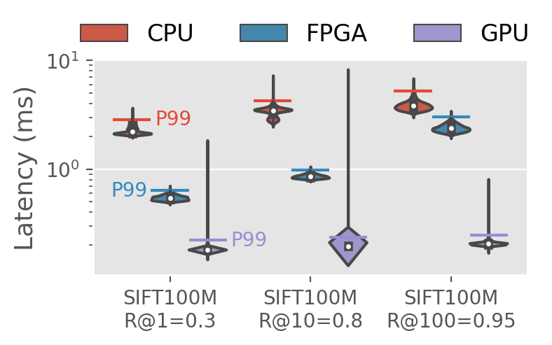
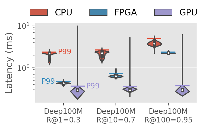
To support low-latency online query processing, we integrate FANNS with a hardware TCP/IP stack (He et al., 2021), such that clients can query the FPGA directly, bypassing the host server. We also compare system scalability of GPUs and FPGAs in this scenario. As the network stack also consumes hardware resources, we rerun the FANNS performance model to generate the best accelerators. We assume the queries already arrive at the host server for CPU and GPU baselines, while for FPGAs, the measurements include the network latency (around five $\mu$ s RTT).

FPGA achieves 2.0 $\sim$ 4.6 $\times$ better P95 latency than the best CPU baseline. Figure 11 captures the latency distributions (Hoefler and Belli, 2015) of each type of hardware. Although showing high tail latency, GPUs still achieve lower median and P95 latency than FPGAs and CPUs due to the much higher flop/s and bandwidth. The FPGA shows much lower latency variance than its counterparts, thanks to the fixed accelerator logic in FPGAs.

FPGAs achieves 5.5 $\times$ and 7.6 $\times$ speedup over GPUs in median and P95 latency in an eight-accelerator setup, as shown in Figure 1. We run the prototype scale-out experiments on a cluster of eight FPGAs. Each FPGA or GPU holds a 100-million vector partition, running the same index (nlist=8192, $m$ =16) to achieve R@10=80%. For FPGAs, we use a CPU server that sends queries to all FPGAs and aggregates the results. For GPUs, Faiss natively supports multi-GPU workload partitioning. FPGAs achieve better scalability thanks to their stable latency distribution, as shown in Figure 11. In contrast, GPUs experience long tail latencies, thus a multi-GPU query is more likely to be constrained by a slow run.

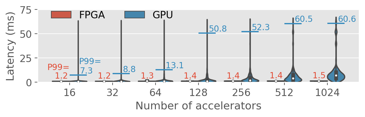
FPGAs are expected to exhibit increasing speedup over GPUs as the search involves more (hundreds or thousands of) accelerators. To extrapolate latency trends beyond eight accelerators, we estimate the latency distribution of large-scale vector search using the following method. The query latency consists of search and network components. We record search latencies of 100K queries on a single FPGA/GPU using the same parameters as the above paragraph. For a distributed query, we randomly sample N_accelerator latency numbers from the latency history and use the highest number as the search latency. We assume the implementation of broadcast/reduce communication collectives follows a binary tree topology. Subsequently, we apply LogGP (Culler et al., 1993; Alexandrov et al., 1995) to model the network latency, using previously reported values measured for InfiniBand using MPI (Hoefler and Moor, 2014; Hoefler et al., 2007): the maximum communication latency between two endpoints is 6.0 $\mu$ s; the constant CPU overhead for sending or receiving a single message is 4.7 $\mu$ s; and the cost per injected byte at the network interface is 0.73 ns/byte. We assume merging partial results from two nodes takes 1.0 $\mu$ s. As shown in Figure 12, FPGA’s P99 latency speedup over GPUs increases from 6.1 $\times$ with 16 accelerators to 42.1 $\times$ with 1024 accelerators, thanks to the low search latency variance on FPGAs.

8. Related Work

To our knowledge, FANNS is the first hardware-algorithm co-design framework for vector search. We introduce related works below.

Vector search on modern hardware. The most popular GPU-accelerated ANN library so far is Faiss developed by Meta (Johnson et al., 2019). The academia has also built several GPU-based ANNS systems (Wieschollek et al., 2016; Chen et al., 2019a, b). Google researchers accelerate exact nearest neighbor search on TPUs and show great performance on one-million-vector datasets (Chern et al., 2022). Lee et al. (2022) propose a fixed ASIC design for PQ supporting arbitrary algorithm parameters.Zhang et al. (2018) implements a variation of the PQ algorithm on FPGAs and focuses on compressing large IVF indexes to fit it to BRAM. Ren et al. (2020) stores full-precision vectors in non-volatile memory to scale up graph-based ANNS, while on-disk ANNS has to be careful with I/O cost (Chen et al., 2021; Jayaram Subramanya et al., 2019; Lejsek et al., 2008).

Vector search in hardware accelerated machine learning systems. Vector search is an essential component in retrieval-augmented language models and recommender systems. For recommender systems, previous work has already explored hardware acceleration using a single FPGA (Jiang et al., 2020), a cluster of FPGAs (Zhu et al., 2021), and hybrid GPU-FPGA clusters (Jiang et al., 2021) in which the FPGA serves as a disaggregated memory node controlling SRAM, HBM, and DDR memory. FANNS can be integrated with them in a single system, enabling the entire candidate generation and click-through rate prediction recommendation pipeline being offloaded to specialized hardware thus allowing high throughput while achieving low service latency.

Vector search algorithms. There are several ways to index the vectors to reduce the number of vectors visited per query. The first category, as introduced in Section 2, is IVF indexes (Sivic and Zisserman, 2003; Babenko and Lempitsky, 2014). The second category is graphs (Malkov et al., 2014; Malkov and Yashunin, 2018; Fu et al., 2017; Sun et al., 2014). The graph should connect nodes (vectors) by edges that present neighborhood relationships. The search starts from an entry point and iteratively traverses the graph until one of the termination conditions is met. The third category is Locality-Sensitive Hashing (LSH) (Gionis et al., 1999; Datar et al., 2004; Huang et al., 2021; Zheng et al., 2016). Each vector is hashed into a bucket that, to some extent, reflects the spatial location of the vector. A search hashes the query and scans the respective bucket. To increase the chance of finding the nearest neighbor, one can create several hash tables and ensemble the search results. LSH is a popular topic for theorists as it provides probabilistic theoretical guarantees. The fourth category is trees (Beis and Lowe, 1997; Silpa-Anan and Hartley, 2008). Though studied in the early days, tree-based structures cannot handle high-dimensional features well due to the curse of dimensionality. Apart from indexing methods, researchers also propose to quantize the vectors to reduce memory footprint and save bandwidth. Product quantization (Jegou et al., 2010; Ge et al., 2013) is the most popular quantization algorithm for ANN search.

9. Conclusion

Commercial search engines are driven by a large-scale vector search system operating on a massive cluster of servers. We introduce FANNS, a scalable FPGA vector search framework that co-designs hardware and algorithm. Our eight-FPGA prototype demonstrates 7.6 $\times$ improvement in P95 latency compared to eight GPUs, with our performance model indicating that this advantage will only increase as more accelerators are employed. The remarkable performance of FANNS lays a robust groundwork for future FPGA integration in data centers, with potential applications spanning large-scale search engines, LLM training, and scientific research in fields such as biomedicine and chemistry.

Acknowledgements.

We would like to thank AMD for their generous donation of the Heterogeneous Accelerated Compute Clusters (HACC) at ETH Zurich (https://systems.ethz.ch/research/data-processing-on-modern-hardware/hacc.html), on which the FPGA experiments were conducted.

References

(1)
int ([n.d.]) [n.d.]. https://www.intel.com/content/www/us/en/software/programmable/sdk-for-opencl/overview.html.
Bin ([n.d.]) [n.d.]. RocksDB in Microsoft Bing. https://blogs.bing.com/Engineering-Blog/october-2021/RocksDB-in-Microsoft-Bing.
viv ([n.d.]) [n.d.]. Vivado High-Level Synthesis. https://www.xilinx.com/products/design-tools/vivado/integration/esl-design.html.
Goo ([n.d.]) [n.d.]. Worldwide visits to Google.com. https://www.statista.com/statistics/268252/web-visitor-traffic-to-googlecom/.
Alexandrov et al. (1995) Albert Alexandrov, Mihai F Ionescu, Klaus E Schauser, and Chris Scheiman. 1995. LogGP: Incorporating long messages into the LogP model—one step closer towards a realistic model for parallel computation. In Proceedings of the seventh annual ACM symposium on Parallel algorithms and architectures. 95–105.
Anagnostou et al. (2020) Panagiotis Anagnostou, Petros Barbas, Aristidis G Vrahatis, and Sotiris K Tasoulis. 2020. Approximate kNN Classification for Biomedical Data. In 2020 IEEE International Conference on Big Data (Big Data). IEEE, 3602–3607.
Babenko and Lempitsky (2014) Artem Babenko and Victor Lempitsky. 2014. The inverted multi-index. IEEE transactions on pattern analysis and machine intelligence 37, 6 (2014), 1247–1260.
Bajusz et al. (2015) Dávid Bajusz, Anita Rácz, and Károly Héberger. 2015. Why is Tanimoto index an appropriate choice for fingerprint-based similarity calculations? Journal of cheminformatics 7, 1 (2015), 1–13.
Batcher (1968) Kenneth E Batcher. 1968. Sorting networks and their applications. In Proceedings of the April 30–May 2, 1968, spring joint computer conference. 307–314.
Beis and Lowe (1997) Jeffrey S Beis and David G Lowe. 1997. Shape indexing using approximate nearest-neighbour search in high-dimensional spaces. In Proceedings of IEEE computer society conference on computer vision and pattern recognition. IEEE, 1000–1006.
Borgeaud et al. (2021) Sebastian Borgeaud, Arthur Mensch, Jordan Hoffmann, Trevor Cai, Eliza Rutherford, Katie Millican, George van den Driessche, Jean-Baptiste Lespiau, Bogdan Damoc, Aidan Clark, et al. 2021. Improving language models by retrieving from trillions of tokens. arXiv preprint arXiv:2112.04426 (2021).
Chen et al. (2021) Qi Chen, Bing Zhao, Haidong Wang, Mingqin Li, Chuanjie Liu, Zengzhong Li, Mao Yang, and Jingdong Wang. 2021. SPANN: Highly-efficient Billion-scale Approximate Nearest Neighbor Search. arXiv preprint arXiv:2111.08566 (2021).
Chen et al. (2019b) Wei Chen, Jincai Chen, Fuhao Zou, Yuan-Fang Li, Ping Lu, Qiang Wang, and Wei Zhao. 2019b. Vector and line quantization for billion-scale similarity search on GPUs. Future Generation Computer Systems 99 (2019), 295–307.
Chen et al. (2019a) Wei Chen, Jincai Chen, Fuhao Zou, Yuan-Fang Li, Ping Lu, and Wei Zhao. 2019a. Robustiq: A robust ann search method for billion-scale similarity search on gpus. In Proceedings of the 2019 on International Conference on Multimedia Retrieval. 132–140.
Chern et al. (2022) Felix Chern, Blake Hechtman, Andy Davis, Ruiqi Guo, David Majnemer, and Sanjiv Kumar. 2022. TPU-KNN: K Nearest Neighbor Search at Peak FLOP/s. arXiv preprint arXiv:2206.14286 (2022).
Covington et al. (2016) Paul Covington, Jay Adams, and Emre Sargin. 2016. Deep neural networks for youtube recommendations. In Proceedings of the 10th ACM conference on recommender systems. 191–198.
Culler et al. (1993) David Culler, Richard Karp, David Patterson, Abhijit Sahay, Klaus Erik Schauser, Eunice Santos, Ramesh Subramonian, and Thorsten Von Eicken. 1993. LogP: Towards a realistic model of parallel computation. In Proceedings of the fourth ACM SIGPLAN symposium on Principles and practice of parallel programming. 1–12.
Datar et al. (2004) Mayur Datar, Nicole Immorlica, Piotr Indyk, and Vahab S Mirrokni. 2004. Locality-sensitive hashing scheme based on p-stable distributions. In Proceedings of the twentieth annual symposium on Computational geometry. 253–262.
de Fine Licht et al. (2020a) Johannes de Fine Licht, Maciej Besta, Simon Meierhans, and Torsten Hoefler. 2020a. Transformations of High-Level Synthesis Codes for High-Performance Computing. IEEE Transactions on Parallel and Distributed Systems 32, 5 (2020), 1014–1029.
de Fine Licht et al. (2020b) Johannes de Fine Licht, Grzegorz Kwasniewski, and Torsten Hoefler. 2020b. Flexible communication avoiding matrix multiplication on FPGA with high-level synthesis. In Proceedings of the 2020 ACM/SIGDA International Symposium on Field-Programmable Gate Arrays. 244–254.
Fu et al. (2017) Cong Fu, Chao Xiang, Changxu Wang, and Deng Cai. 2017. Fast approximate nearest neighbor search with the navigating spreading-out graph. arXiv preprint arXiv:1707.00143 (2017).
Ge et al. (2013) Tiezheng Ge, Kaiming He, Qifa Ke, and Jian Sun. 2013. Optimized product quantization. IEEE transactions on pattern analysis and machine intelligence 36, 4 (2013), 744–755.
Gionis et al. (1999) Aristides Gionis, Piotr Indyk, Rajeev Motwani, et al. 1999. Similarity search in high dimensions via hashing. In Vldb, Vol. 99. 518–529.
Guu et al. (2020) Kelvin Guu, Kenton Lee, Zora Tung, Panupong Pasupat, and Ming-Wei Chang. 2020. Realm: Retrieval-augmented language model pre-training. arXiv preprint arXiv:2002.08909 (2020).
He et al. (2021) Zhenhao He, Dario Korolija, and Gustavo Alonso. 2021. EasyNet: 100 Gbps Network for HLS. In 2021 31th International Conference on Field Programmable Logic and Applications (FPL).
Hoefler and Belli (2015) Torsten Hoefler and Roberto Belli. 2015. Scientific benchmarking of parallel computing systems: twelve ways to tell the masses when reporting performance results. In Proceedings of the international conference for high performance computing, networking, storage and analysis. 1–12.
Hoefler et al. (2007) Torsten Hoefler, Andre Lichei, and Wolfgang Rehm. 2007. Low-overhead LogGP parameter assessment for modern interconnection networks. In 2007 IEEE International Parallel and Distributed Processing Symposium. IEEE, 1–8.
Hoefler and Moor (2014) Torsten Hoefler and Dmitry Moor. 2014. Energy, memory, and runtime tradeoffs for implementing collective communication operations. Supercomputing frontiers and innovations 1, 2 (2014), 58–75.
Huang et al. (2020) Jui-Ting Huang, Ashish Sharma, Shuying Sun, Li Xia, David Zhang, Philip Pronin, Janani Padmanabhan, Giuseppe Ottaviano, and Linjun Yang. 2020. Embedding-based retrieval in facebook search. In Proceedings of the 26th ACM SIGKDD International Conference on Knowledge Discovery & Data Mining. 2553–2561.
Huang et al. (2014) Muhuan Huang, Kevin Lim, and Jason Cong. 2014. A scalable, high-performance customized priority queue. In 2014 24th International Conference on Field Programmable Logic and Applications (FPL). IEEE, 1–4.
Huang et al. (2021) Qiang Huang, Yifan Lei, and Anthony KH Tung. 2021. Point-to-Hyperplane Nearest Neighbor Search Beyond the Unit Hypersphere. In Proceedings of the 2021 International Conference on Management of Data. 777–789.
Jayaram Subramanya et al. (2019) Suhas Jayaram Subramanya, Fnu Devvrit, Harsha Vardhan Simhadri, Ravishankar Krishnawamy, and Rohan Kadekodi. 2019. Diskann: Fast accurate billion-point nearest neighbor search on a single node. Advances in Neural Information Processing Systems 32 (2019).
Jegou et al. (2010) Herve Jegou, Matthijs Douze, and Cordelia Schmid. 2010. Product quantization for nearest neighbor search. IEEE transactions on pattern analysis and machine intelligence 33, 1 (2010), 117–128.
Jiang et al. (2020) Wenqi Jiang, Zhenhao He, Shuai Zhang, Thomas B Preußer, Kai Zeng, Liang Feng, Jiansong Zhang, Tongxuan Liu, Yong Li, Jingren Zhou, et al. 2020. MicroRec: Accelerating Deep Recommendation Systems to Microseconds by Hardware and Data Structure Solutions. arXiv preprint arXiv:2010.05894 (2020).
Jiang et al. (2021) Wenqi Jiang, Zhenhao He, Shuai Zhang, Kai Zeng, Liang Feng, Jiansong Zhang, Tongxuan Liu, Yong Li, Jingren Zhou, Ce Zhang, et al. 2021. Fleetrec: Large-scale recommendation inference on hybrid gpu-fpga clusters. In Proceedings of the 27th ACM SIGKDD Conference on Knowledge Discovery & Data Mining. 3097–3105.
Jiang et al. (2023) Wenqi Jiang, Dario Korolija, and Gustavo Alonso. 2023. Data Processing with FPGAs on Modern Architectures. In Companion of the 2023 International Conference on Management of Data. 77–82.
Johnson et al. (2019) Jeff Johnson, Matthijs Douze, and Hervé Jégou. 2019. Billion-scale similarity search with gpus. IEEE Transactions on Big Data (2019).
Karpukhin et al. (2020) Vladimir Karpukhin, Barlas Oğuz, Sewon Min, Patrick Lewis, Ledell Wu, Sergey Edunov, Danqi Chen, and Wen-tau Yih. 2020. Dense passage retrieval for open-domain question answering. arXiv preprint arXiv:2004.04906 (2020).
Khattab and Zaharia (2020) Omar Khattab and Matei Zaharia. 2020. Colbert: Efficient and effective passage search via contextualized late interaction over bert. In Proceedings of the 43rd International ACM SIGIR conference on research and development in Information Retrieval. 39–48.
Lee et al. (2022) Yejin Lee, Hyunji Choi, Sunhong Min, Hyunseung Lee, Sangwon Beak, Dawoon Jeong, Jae W Lee, and Tae Jun Ham. 2022. ANNA: Specialized Architecture for Approximate Nearest Neighbor Search. In 2022 IEEE International Symposium on High-Performance Computer Architecture (HPCA). IEEE, 169–183.
Leiserson (1979) Charles E Leiserson. 1979. Systolic Priority Queues. Technical Report. CARNEGIE-MELLON UNIV PITTSBURGH PA DEPT OF COMPUTER SCIENCE.
Lejsek et al. (2008) Herwig Lejsek, Friðrik Heiðar Ásmundsson, Björn Þór Jónsson, and Laurent Amsaleg. 2008. NV-Tree: An efficient disk-based index for approximate search in very large high-dimensional collections. IEEE Transactions on Pattern Analysis and Machine Intelligence 31, 5 (2008), 869–883.
Lewis et al. (2020) Patrick Lewis, Ethan Perez, Aleksandra Piktus, Fabio Petroni, Vladimir Karpukhin, Naman Goyal, Heinrich Küttler, Mike Lewis, Wen-tau Yih, Tim Rocktäschel, et al. 2020. Retrieval-augmented generation for knowledge-intensive nlp tasks. Advances in Neural Information Processing Systems 33 (2020), 9459–9474.
Malkov et al. (2014) Yury Malkov, Alexander Ponomarenko, Andrey Logvinov, and Vladimir Krylov. 2014. Approximate nearest neighbor algorithm based on navigable small world graphs. Information Systems 45 (2014), 61–68.
Malkov and Yashunin (2018) Yu A Malkov and Dmitry A Yashunin. 2018. Efficient and robust approximate nearest neighbor search using hierarchical navigable small world graphs. IEEE transactions on pattern analysis and machine intelligence 42, 4 (2018), 824–836.
Mueller et al. (2012) Rene Mueller, Jens Teubner, and Gustavo Alonso. 2012. Sorting networks on FPGAs. The VLDB Journal 21, 1 (2012), 1–23.
Neumann et al. (2019) Mark Neumann, Daniel King, Iz Beltagy, and Waleed Ammar. 2019. ScispaCy: fast and robust models for biomedical natural language processing. arXiv preprint arXiv:1902.07669 (2019).
Papaphilippou et al. (2018) Philippos Papaphilippou, Chris Brooks, and Wayne Luk. 2018. Flims: Fast lightweight merge sorter. In 2018 International Conference on Field-Programmable Technology (FPT). IEEE, 78–85.
Papaphilippou et al. (2020) Philippos Papaphilippou, Chris Brooks, and Wayne Luk. 2020. An Adaptable High-Throughput FPGA Merge Sorter for Accelerating Database Analytics. In 2020 30th International Conference on Field-Programmable Logic and Applications (FPL). IEEE, 65–72.
Ren et al. (2020) Jie Ren, Minjia Zhang, and Dong Li. 2020. Hm-ann: Efficient billion-point nearest neighbor search on heterogeneous memory. Advances in Neural Information Processing Systems 33 (2020), 10672–10684.
Salamat et al. (2021) Sahand Salamat, Armin Haj Aboutalebi, Behnam Khaleghi, Joo Hwan Lee, Yang Seok Ki, and Tajana Rosing. 2021. NASCENT: Near-Storage Acceleration of Database Sort on SmartSSD. In The 2021 ACM/SIGDA International Symposium on Field-Programmable Gate Arrays. 262–272.
Silpa-Anan and Hartley (2008) Chanop Silpa-Anan and Richard Hartley. 2008. Optimised KD-trees for fast image descriptor matching. In 2008 IEEE Conference on Computer Vision and Pattern Recognition. IEEE, 1–8.
Sivic and Zisserman (2003) Josef Sivic and Andrew Zisserman. 2003. Video Google: A text retrieval approach to object matching in videos. In Computer Vision, IEEE International Conference on, Vol. 3. IEEE Computer Society, 1470–1470.
Song et al. (2016) Wei Song, Dirk Koch, Mikel Luján, and Jim Garside. 2016. Parallel hardware merge sorter. In 2016 IEEE 24th Annual International Symposium on Field-Programmable Custom Computing Machines (FCCM). IEEE, 95–102.
Suchal and Návrat (2010) Ján Suchal and Pavol Návrat. 2010. Full text search engine as scalable k-nearest neighbor recommendation system. In IFIP International Conference on Artificial Intelligence in Theory and Practice. Springer, 165–173.
Sun et al. (2014) Yifang Sun, Wei Wang, Jianbin Qin, Ying Zhang, and Xuemin Lin. 2014. SRS: solving c-approximate nearest neighbor queries in high dimensional euclidean space with a tiny index. Proceedings of the VLDB Endowment (2014).
Wei et al. (2020) Chuangxian Wei, Bin Wu, Sheng Wang, Renjie Lou, Chaoqun Zhan, Feifei Li, and Yuanzhe Cai. 2020. AnalyticDB-V: a hybrid analytical engine towards query fusion for structured and unstructured data. Proceedings of the VLDB Endowment 13, 12 (2020), 3152–3165.
Wieschollek et al. (2016) Patrick Wieschollek, Oliver Wang, Alexander Sorkine-Hornung, and Hendrik Lensch. 2016. Efficient large-scale approximate nearest neighbor search on the gpu. In Proceedings of the IEEE Conference on Computer Vision and Pattern Recognition. 2027–2035.
Willett (2014) Peter Willett. 2014. The calculation of molecular structural similarity: principles and practice. Molecular informatics 33, 6-7 (2014), 403–413.
Woodbridge et al. (2016) Jonathan Woodbridge, Bobak Mortazavi, Alex AT Bui, and Majid Sarrafzadeh. 2016. Improving biomedical signal search results in big data case-based reasoning environments. Pervasive and mobile computing 28 (2016), 69–80.
Xiong et al. (2020) Lee Xiong, Chenyan Xiong, Ye Li, Kwok-Fung Tang, Jialin Liu, Paul Bennett, Junaid Ahmed, and Arnold Overwijk. 2020. Approximate nearest neighbor negative contrastive learning for dense text retrieval. arXiv preprint arXiv:2007.00808 (2020).
Zhang et al. (2018) Jialiang Zhang, Soroosh Khoram, and Jing Li. 2018. Efficient large-scale approximate nearest neighbor search on OpenCL FPGA. In Proceedings of the IEEE Conference on Computer Vision and Pattern Recognition. 4924–4932.
Zheng et al. (2016) Yuxin Zheng, Qi Guo, Anthony KH Tung, and Sai Wu. 2016. Lazylsh: Approximate nearest neighbor search for multiple distance functions with a single index. In Proceedings of the 2016 International Conference on Management of Data. 2023–2037.
Zhu et al. (2021) Yu Zhu, Zhenhao He, Wenqi Jiang, Kai Zeng, Jingren Zhou, and Gustavo Alonso. 2021. Distributed recommendation inference on fpga clusters. In 2021 31st International Conference on Field-Programmable Logic and Applications (FPL). IEEE, 279–285.

Appendix A Artifact Description

We introduce FANNS, an end-to-end and scalable vector search framework on FPGAs. Given a user-provided recall requirement on a dataset and a hardware resource budget, FANNS automatically co-designs hardware and algorithm, subsequently generating the corresponding accelerator. The framework also supports scale-out by incorporating a hardware TCP/IP stack in the accelerator.

We use the following open-source software and commercial hardware in the experiments. The experimental results should be easily reproducible on the same hardware.

A.1. Hardware.

For CPU experiments, we use an m5.4xlarge CPU server on AWS. The server contains 16 vCPUs of Intel(R) Xeon(R) Platinum 8259CL @ 2.50GHz (Cascade Lake, 14nm technology) and 64 GB of DDR4 memory. For GPU experiments, we use a p3.24xlarge GPU server on AWS. It contains eight NVIDIA V100 GPUs manufactured by the TSMC 12 nm FFN (FinFET NVIDIA) technology. Each GPU has 5,120 CUDA cores and 32 GB HBM2. For FPGA experiments, we use Xilinx Alveo U55c FPGA fabricated with TSMC’s 16nm process. Each FPGA contains 1.3M LUTs, 9K DSPs, 40MB on-chip memory, and 16 GB HBM. We use a cluster of FPGAs for scale-out experiments, and all the U55c FPGAs are connected to the same switch.

A.2. Software.

We use Faiss 1.7.1 for both CPU and GPU experiments. The CUDA version of the GPU server is 11.3. For FPGA experiments, we develop the accelerators using Vitis HLS 2022.1.

Appendix B Artifact Evaluation

The code of FPGA accelerators with/without the network stack as well as the CPU/GPU baseline evaluations are available at: https://github.com/WenqiJiang/SC-ANN-FPGA. We only apply for the availability badge because the HACC FPGA cluster at ETH Zurich does not allow anonymous access for reproducibility evaluation.

The repository contains three folders with documented execution flow:

•

The CPU_GPU_baselines folder contains all the CPU and GPU baseline experiments. It also contains part of the co-design formula – we use Faiss to evaluate the relationship between index, nprobe, and recall on a given dataset.
•

The FPGA_local folder contains all the CD-ANN programs without the network stack. Its performance_model sub-directory contains the performance and resource consumption models. A user can use the programs in it to predict the best hardware design given a certain recall goal on a dataset. The code_generation sub-directory can generate the ready-to-compile FPGA code given a hardware setting, which is either predicted by the performance model or set by the user manually. The generated_projects sub-directory contains all the generated FPGA accelerator code that we evaluated in the experiments.
•

The FPGA_with_network folder contains all the FPGA accelerators that we evaluated with the network stack. The FPGA kernels are located in the kernel/user_kernel sub-directory. The CPU client programs are in the CPU_program sub-directory.

It will take a significant amount of time to reproduce all results. Training the indexes can be costly (around two hours per index), given that we trained 18 indexes in the paper. Once the indexes are trained, it should take less than two hours on CPUs and GPUs to reproduce the performance. The FPGA compilation can take around ten hours per design, which is costly because we have more than ten designs to form the experiments. Executing an FPGA program should take less than a minute.

The reproduced results are expected to be identical to the paper, given that we already reported performance on multiple runs and characterized the error bars in throughput experiments as well as latency distributions in latency experiments.