Hyperbolic Active Learning for Semantic Segmentation under Domain Shift

Abstract

We introduce a hyperbolic neural network approach to pixel-level active learning for semantic segmentation, and propose a novel geometric interpretation of the hyperbolic geometry that arises bottom-up from the statistics of the data. In our formulation the hyperbolic radius emerges as an estimator of the unexplained class complexity, which encompasses the class intrinsic complexity and its scarcity in the dataset. The unexplained class complexity serves as a metric indicating the likelihood that acquiring a particular pixel would contribute to enhancing the data information. We combine this quantity with prediction uncertainty to compute an acquisition score that identifies the most informative pixels for oracle annotation. Our proposed HALO (Hyperbolic Active Learning Optimization) sets a new state-of-the-art in active learning for semantic segmentation under domain shift, and surpasses the supervised domain adaptation performance while only using a small portion of labels (i.e., 1%). We perform extensive experimental analysis based on two established benchmarks, i.e. GTAV $\rightarrow$ Cityscapes and SYNTHIA $\rightarrow$ Cityscapes, and we additionally test on Cityscape $\rightarrow$ ACDC under adverse weather conditions.

1 Introduction

Dense prediction tasks, such as semantic segmentation (SS), are important in applications such as self-driving cars, manufacturing, and medicine. However, these tasks necessitate pixel-wise annotations, which can incur substantial costs and time inefficiencies (Cordts et al., 2016). Previous methods (Xie et al., 2022a; Vu et al., 2019; Shin et al., 2021b; a; Ning et al., 2021) have addressed this labeling challenge via domain adaptation, capitalizing on large source datasets for pre-training and domain-adapting with few target annotations (Ben-David et al., 2010). Most recently, active domain adaptation (ADA) has emerged as an effective strategy, i.e. annotating only a small set of target pixels in successive labelling rounds (Ning et al., 2021).

State-of-the-art (SoA) ADA relies on prediction uncertainty and pseudo-labels as the core strategy for active learning (AL) data acquisition (Shin et al., 2021b; Wu et al., 2022; Xie et al., 2022a). The current best performer (Xie et al., 2022a) introduces a region impurity score to prioritize the annotation of pixels likely at the class boundaries as a data acquisition strategy. But the pixels at the class boundaries are not necessarily the most informative and annotating only those degrades performance, as we confirm with an oracular study. Here, we argue that the scarcity of labels for certain class prototypical appearances and the intrinsic complexity of classes are better cues for an AL data acquisition strategy.

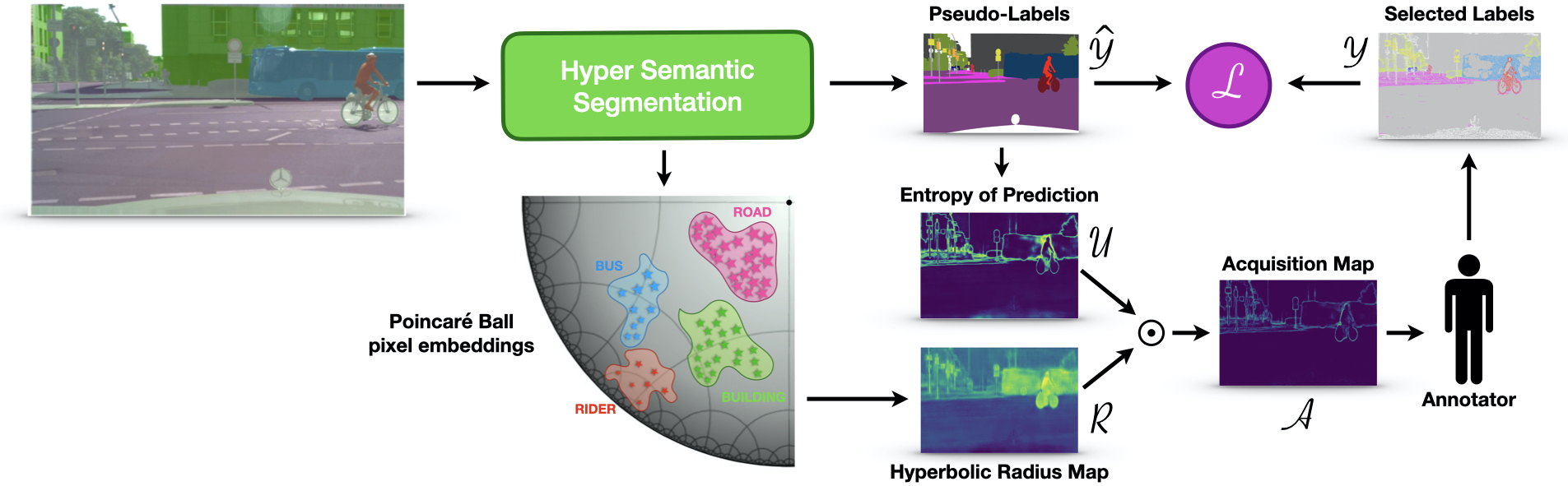
Figure 1: Overview of HALO. Pixels are encoded into the hyperbolic Poincaré ball and classified in the pseudo-label $\mathcal{\hat{Y}}$. The hyperbolic radius of the pixel embeddings defines the new hyperbolic score map $\mathcal{R}$. The uncertainty map $\mathcal{U}$ is extracted as the entropy of the classification probabilities. Combining $\mathcal{R}$ and $\mathcal{U}$ we define the data acquisition map $\mathcal{A}$, which is used to query new labels $\mathcal{Y}$.

We propose Hyperbolic Active Learning Optimization (HALO), the first hyperbolic framework for AL, and a novel geometric interpretation of the hyperbolic radius. The SoA hyperbolic SS model  (Atigh et al., 2022) trains with class hierarchies, which they manually define. As a result, their hyperbolic radius represents the parent-to-child hierarchical relations in the Poincaré ball. We adopt  Atigh et al. (2022), but we find that hierarchies do not emerge naturally when they are not enforced at training time. E.g., in HALO road and building classes are closer to the center of the ball, while person and rider have larger radii. This class arrangement also defies the interpretation of the hyperbolic radius as a proxy for uncertainty, which emerged from metric learning hyperbolic studies (Ermolov et al., 2022; Franco et al., 2023), as road and building classes are not less uncertain. So neither interpretation explains the learned radii in the case of hierarchy-free hyperbolic SS.

We identify a novel interpretation of the hyperbolic geometry, wherein the hyperbolic radius serves as a proxy for the unexplained class complexity. This concept encompasses two facets: the intrinsic class complexity (for instance, a rider is more challenging to classify than the road), and the quantity of class labels the model has been exposed to during training (the rider class has fewer labels than road). Consider the HALO pipeline illustrated in Figure  1 and the circular sector representing the Poincaré ball, where pixels from various classes are mapped. HALO learns a manifold where the distance of a class from the center is directly proportional to the unexplained class complexity. In Sec. 4 we show how the hyperbolic radius emerges bottom-up from data statistics as a proxy for the unexplained class complexity. Specifically, the radius correlates with the inherent complexity of the class and the scarcity of labeled data for it. In HALO, this motivates us to use the radius to directly acquire the most informative pixels during the active learning round.

We demonstrate the efficacy of our approach through extensive benchmarking on well-established datasets for SS via ADA as GTAV $\rightarrow$ Cityscapes, SYNTHIA $\rightarrow$ Cityscapes, and additionally testing on Cityscapes $\rightarrow$ ACDC under adverse weather conditions. HALO sets a new SoA on all the benchmarks and it surpasses the supervised domain adaptation baseline. Our framework also introduces a novel technique for enhancing the stability of hyperbolic training, which we refer to as Hyperbolic Feature Reweighting (HFR), cf. Sec. 5. Our code will be released.

In summary, our contributions include:

1. Presenting a novel geometric interpretation of the hyperbolic radius as a proxy for the concept of unexplained class complexity;

2. Introducing hyperbolic neural networks in AL and a novel pixel-based data acquisition score based on the hyperbolic radius;

3. Conducting a comprehensive analysis to validate both the concept and the algorithm while setting a new state-of-the-art across all ADA benchmarks for SS.

2 Related Works

Hyperbolic Representation Learning (HRL)  Hyperbolic geometry has been extensively used to capture embeddings of tree-like structures (Nickel & Kiela, 2017; Chami et al., 2020) with low distortion Sala et al. (2018); Sarkar (2012). Since the seminal work of Ganea et al. (2018) on Hyperbolic Neural Networks (HNN), approaches have successfully combined hyperbolic geometry with model architectures ranging from convolutional (Shimizu et al., 2020) to attention-based (Gulcehre et al., 2018), including graph neural networks (Liu et al., 2019; Chami et al., 2019) and, most recently, vision transformers (Ermolov et al., 2022). There are two leading interpretations of the hyperbolic radius in hyperbolic space: as a measure of the prediction uncertainty (Chen et al., 2022; Ermolov et al., 2022; Franco et al., 2023) or as the hierarchical parent-to-child relation (Nickel & Kiela, 2017; Tifrea et al., 2018; Surís et al., 2021; Ermolov et al., 2022; Atigh et al., 2022). Our work builds on the SoA hyperbolic semantic segmentation method of Atigh et al. (2022), which enforces hierarchical labels and training objectives. However, when training hierarchy-free for ADA, as we do, the hierarchical interpretation does not apply; nor is the uncertainty viewpoint applicable. To the best of our knowledge, we are the first to propose a third interpretation for the HNNs connecting the hyperbolic space density to the semantic class recognition difficulty.

Active Learning (AL)  The number of annotations required for dense tasks such as semantic segmentation can be costly and time-consuming. Active learning balances the labeling efforts and performance, selecting the most informative pixels in successive learning rounds. Strategies for active learning are based on uncertainty sampling (Gal et al., 2017; Wang & Shang, 2014; Wang et al., 2016), diversity sampling (Ash et al., 2019; Kirsch et al., 2019; Sener & Savarese, 2017; Wu et al., 2021) or a combination of both (Sinha et al., 2019; Xie et al., 2022b; Prabhu et al., 2021; Xie et al., 2022a). For the case of AL in semantic segmentation, EqualAL (Golestaneh & Kitani, 2020) incorporates the self-supervisory signal of self-consistency to mitigate the overfitting of scenarios with limited labeled training data. Labor (Shin et al., 2021b) selects the most representative pixels within the generation of an inconsistency mask. PixelPick (Shin et al., 2021a) prioritizes the identification of specific pixels or regions over labeling the entire image. Mittal et al. (2023) explores the effect of data distribution, semi-supervised learning, and labeling budgets. We are the first to leverage the hyperbolic radius as a proxy for the most informative pixels to label next.

Active Domain Adaptation (ADA)  Domain Adaptation (DA) involves learning from a source data distribution and transferring that knowledge to a target dataset with a different distribution. Recent advancements in DA for semantic segmentation have utilized unsupervised (UDA) (Hoffman et al., 2018; Vu et al., 2019; Yang & Soatto, 2020; Liu et al., 2020; Mei et al., 2020; Liu et al., 2021) and semi-supervised (SSDA) (French et al., 2017; Saito et al., 2019; Singh, 2021; Jiang et al., 2020) learning techniques. However, challenges such as noise and label bias still pose limitations on the performance of DA methods. Active Domain Adaptation (ADA) aims to reduce the disparity between source and target domains by actively selecting informative data points from the target domain (Su et al., 2020; Fu et al., 2021; Singh et al., 2021; Shin et al., 2021b), which are subsequently labeled by human annotators. In semantic segmentation, Ning et al. (2021) propose a multi-anchor strategy to mitigate the distortion between the source and target distributions. The recent study of Xie et al. (2022a) shows the advantages of region-based selection in terms of region impurity and prediction uncertainty scores, compared to pixel-based approaches. By contrast, we show that selecting just from contours limits performance, and that unexplained class complexity is a better objective, as estimated by the hyperbolic radius.

3 Background

We provide preliminaries on two techniques that HALO builds upon: Hyperbolic Image Segmentation  (Atigh et al., 2022) and Active Domain Adaptation.

Hyperbolic Neural Networks

We operate in the Poincaré ball hyperbolic space. We define it as the pair $(\mathbb{D}_{c}^{N},g^{\mathbb{D}_{c}})$ where $\mathbb{D}_{c}^{N}=\{x\in\mathbb{R}^{N}:c\|x\|<1\}$ is the manifold and $g_{x}^{\mathbb{D}_{c}}=(\lambda_{x}^{c})^{2}g^{\mathbb{E}}$ is the associated Riemannian metric, $-c$ is the curvature, $\lambda_{x}^{c}=\frac{2}{1-c\|x\|^{2}}$ is the conformal factor and $g^{\mathbb{E}}=\mathbb{I}^{N}$ is the Euclidean metric tensor. Hyperbolic neural networks first extract a feature vector $v$ in Euclidean space, which is subsequently projected into the Poincaré ball via exponential map:

$$exp_{x}^{c}(v)=x\oplus_{c}\left(\frac{v}{\sqrt{c}\|v\|}tanh\left(\sqrt{c}\frac{\lambda_{x}^{c}\|v\|}{2}\right)\right)$$ (1)

where $x\in\mathbb{D}_{c}^{N}$ is the anchor and $\oplus_{c}$ is the Möbius hyperbolic addition. The latter is defined for two hyperbolic vectors $h,w$ as follows:

$$h\oplus_{c}w=\frac{(1+2c\langle h,w\rangle+c\|w\|^{2})v+(1-c\|h\|^{2})w}{1+2c\langle h,w\rangle+c^{2}\|h\|^{2}\|w\|^{2}}$$ (2)

We define the hyperbolic radius of the embedding $h\in\mathbb{D}_{c}^{N}$ as the Poincaré distance (See Eq. A1 in Appendix A.4) from the origin of the ball:

$$d(h,0)=\frac{2}{\sqrt{c}}tanh^{-1}\left(\sqrt{c}\|h\|\right),$$ (3)

We propose to use the hyperbolic radius of the pixel embeddings as a novel data acquisition strategy. This is motivated by a novel geometric interpretation of the hyperbolic radius, which we support with experimental evidence in this section.

Hyperbolic Multinomial Logistic Regression (MLR)

Following Ganea et al. (2018), to classify an image feature $z_{i}\in\mathbb{R}^{N}$ we project it onto the Poincaré ball $h_{i}=\exp_{x}^{c}(z_{i})\in\mathbb{D}_{c}^{N}$ and classify with a number of hyperplanes $H_{y}^{c}$ (known as ”gyroplanes”) for each class $y$:

$$H_{y}^{c}=\{h_{i}\in\mathbb{D}_{c}^{N},\langle-p_{y}\oplus_{c}h_{i},w_{y}\rangle\},$$ (4)

where, $p_{y}$ represents the gyroplane offset, and $w_{y}$ represents the orientation for class $y$. The distance between a Poincaré ball embedding $h_{i}$ and the gyroplane $H_{y}^{c}$ is given by:

$$d(h_{i},H_{y}^{c})=\frac{1}{\sqrt{c}}sinh^{-1}\left(\frac{2\sqrt{c}\langle-p_{y}\oplus_{c}h_{i},w_{y}\rangle}{(1-c\|-p_{y}\oplus_{c}h_{i}\|^{2})\|w_{y}\|}\right),$$ (5)

Based on this distance, we define the likelihood as $p(\hat{y}_{i}=y|h_{i})\propto exp(\zeta_{y}(h_{i}))$ where $\zeta_{y}(h_{i})=\lambda_{p_{y}}^{c}\|w_{y}\|d(h_{i},H_{y}^{c})$ is the logit for the $y$ class.

ADA for Semantic Segmentation

The task aims to transfer knowledge from a source labeled dataset $\mathcal{S}=(X_{s},Y_{s})$ to a target unlabeled dataset $\mathcal{T}=(X_{t},Y_{t})$, where $X$ represents an image and $Y$ the corresponding annotation map. $Y_{s}$ is given, $Y_{t}$ is initially the empty set $\emptyset$. Adhering to the ADA protocol (Xie et al., 2022a; Wu et al., 2022; Shin et al., 2021b), target annotations are incrementally added in rounds, subject to a predefined budget, upon querying an annotator. Each pixel is assigned a priority score using a predefined acquisition map $\mathcal{A}$. Labels are added to $Y_{s}$ in each AL round by selecting pixels from $\mathcal{A}$ with higher scores, in accordance with the budget. The entire architecture undergoes end-to-end training, with back-propagation incorporating estimates $\hat{Y}_{s}$ and $\hat{Y}_{t}$ from the per-pixel cross-entropy loss $\mathcal{L}({\hat{Y}_{s},\hat{Y}_{t}},{Y_{s},Y_{t}})$.

Setup  Atigh et al. (2022) has been the first to demonstrate a performance of hyperbolic SS on par with Euclidean. They proceed by mapping pixel embeddings onto a hyperbolic space, where they classify by hyperbolic multinomial logistic regression. We assume to have pre-trained the hyperbolic image segmenter of Atigh et al. (2022) on the source dataset GTAV (Richter et al., 2016) and to have domain-adapted it to the target dataset Cityscape (Cordts et al., 2016) with 5 rounds of AL, each adding 1% of the target labels. We assume to have followed the HALO pipeline of Fig. 1, which we detail in Sec. 5. The following section considers the radii of the hyperbolic pixel embeddings, for which statistics are computed on the Cityscape validation set.

4 Hyperbolic Radius and the Unexplained Class Complexity

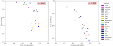
Figure 2: (a) Plot of average per-class radii of pixel embeddings Vs. class accuracies; (b) Plot of per-class radii of pixel embeddings Vs. the percentage of per-class target pixels.

In Sec. 4.1 we interpret the emerging properties of hyperbolic radius, and we compare with the interpretations in literature in Sec. 4.2.

4.1 Emerging Properties of the Hyperbolic Radius

What does the hyperbolic radius represent?  Fig. 2a illustrates the correlation between the per-class average hyperbolic radius and the relative class SS accuracy. They correlate negatively with a significant $\rho=-0.605$. So classes with larger hyperbolic radii have lower performance and are likely more difficult to recognize, more complex. E.g. road has large accuracy and small radius, motocycle has lower accuracy and larger radius. Fig. 2b shows the correlation between the average class hyperbolic radius and the percentage of pixel labels for each class relative to the total number of pixels in the dataset. The correlation is substantial ($\rho=-0.899$), so classes with larger hyperbolic radii such as motocycle are rare in the target dataset, while at lower hyperbolic radii we have more frequent classes such as road. We conclude that the hyperbolic radius indicates the difficulty in recognizing a class, as a consequence of the class complexity and its label scarcity. Building upon this evidence, in Sec. 5, we introduce a novel acquisition score based on the hyperbolic radius to select pixels from classes that are inherently complex and rarer in the target dataset.

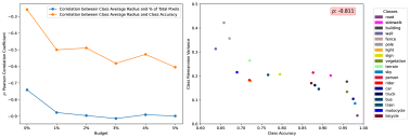
Figure 3: (a) AL evolution of the correlations between the class average radius Vs.  SS accuracy (orange), the correlations between the class average radius Vs.  per class % of total pixels (blue);
(b) Plot of class accuracies Vs. per class Riemannian variance. See Sec. 4 for details.

How does learning the hyperbolic manifold of the pixels embeddings proceed?  Fig. 3a illustrates the evolution, during the active learning rounds, of the correlations between the per-class average radius and two quantities: the classification accuracy (orange), and the percentage of pixels belonging to the specified class in relation to the overall pixel count within the target dataset (blue). During training, both the correlations of the radius Vs. accuracy and the radius Vs. % of total pixels per class grow in module, confirming that the model progressively learns hyperbolic radii, indicative of the recognition difficulty of the class, based on the inherent complexity and label scarcity. The more HALO proceeds, the more the model is aware of what it does not know, i.e. HALO estimates what pixels it considers complex, which makes the best acquisition strategy.

Novel geometric interpretation of the hyperbolic radius  Figure 3b complements the findings by plotting the class accuracies Vs. the Riemannian variance (see Appendix A.4) of radii for each class. The latter generalizes the Euclidean variance, taking into consideration the increasing Poincaré ball density at larger radii. The correlation of accuracies Vs. Riemannian variance is significant ($\rho=-0.811$). So more difficult classes such as pole which have lower accuracy, also have the larger Riemannian variance, so the largest effective volume available. We conclude that the model accomplishes classification on the hyperbolic space by placing more complex classes at larger radii, where the space is denser and there is more volume to model them.

4.2 Comparing interpretations of the hyperbolic radius

It emerges from our analysis that larger radii are assigned to classes that are more difficult to recognize, for their inherent complexity and their label scarcity. Earlier work has explained the hyperbolic radius in terms of uncertainty or hierarchies. Techniques from the former (Chen et al., 2022; Ermolov et al., 2022; Franco et al., 2023) consider that the larger hyperbolic radii indicate more certain and unambiguous samples. This is typical of hyperbolic metric learning-based approaches, whereby the larger radius results in an exponentially larger matching penalty due to the employed Poincaré distance (See Eq. A1 in Appendix A.4). We argue that this yields a self-normalizing learning objective, effectively making the radius proportional to the errors, as those techniques show. Methods in favor of a hierarchical explanation (Nickel & Kiela, 2017; Tifrea et al., 2018; Surís et al., 2021; Ermolov et al., 2022; Atigh et al., 2022) consider hierarchical datasets, labeling, and classification objective functions. Hierarchies naturally align with the growing volume in the Poincaré ball, so children nodes from different parents are mapped further from each other than from their parents. Learning under hierarchical constraints results in leaf classes closer to the ball edge, and moving between them passes via their parents at lower hyperbolic radii. Our hyperbolic SS model is derived from Atigh et al. (2022) but it differs in the geometric meaning of the hyperbolic radii of pixel embeddings. Our novel interpretation may emerge due to the use of the hyperbolic multinomial logistic regression objective without the enforced label hierarchies.

Figure 4: (a) Original image; (b) Radius map depicting the hyperbolic radii of pixel embeddings; (c) Pixels (yellow) that have been selected for data acquisition. See Sec. 5 for details;
(d) HALO prediction; (e) Ground Truth annotations. Zoom in for the details.

5 Hyperbolic Active Learning Optimization (HALO)

This section outlines the HALO framework, which is founded on the novel interpretation of hyperbolic geometry. In Sec. 5.1 we review the HALO pipeline. In Sec. 5.2 we delve into the novel AL acquisition strategy based on the hyperbolic radius. In Sec. 5.3 we present our proposition for fixing the training instability of the hyperbolic framework.

5.1 Halo pipeline

Let us consider Fig. 1. In the training phase, we follow the hyperbolic semantic segmentation approach proposed by Atigh et al. (2022). This involves processing images into pixel embeddings using an encoder followed by expmap, projecting them onto the Poincaré ball. Pseudo-labels are then generated through hyperbolic multinomial logistic regression (Hyper MLR), and the cross-entropy loss is computed based on the target labels chosen in previous rounds of active learning.

At the conclusion of each training cycle, active learning is employed to identify the most informative pixels for annotation. Utilizing pixel embeddings, we estimate the hyperbolic radius $\mathcal{R}$ (as detailed in Sec. 4 and illustrated in Fig. 4b). Concurrently, predicted classification probabilities are used to compute pixel uncertainties $\mathcal{U}$, a technique inspired by prior works such as Paul et al. (2020); Shin et al. (2021a); Wang & Shang (2014); Wang et al. (2016); Xie et al. (2022a). New labels are then chosen based on a data acquisition score $\mathcal{A}$ (as depicted in Fig. 4c), calculated as the element-wise product of $\mathcal{R}$ and $\mathcal{U}$, and these labels are subsequently integrated into the training set. Note that the new labels are both at the boundaries and within, in areas with the largest inaccuracies (compare Fig. 4d and 4e). The rest of the ADA pipeline is as described in Sec. 3.

5.2 Novel data acquisition strategy

The acquisition score of each pixel in an image is formulated as the element-wise multiplication of the hyperbolic radii $\mathcal{R}$ and the uncertainties $\mathcal{U}$, i.e. $\mathcal{A}=\mathcal{R}\odot\mathcal{U}$. The radius $\mathcal{R}^{(i,j)}$ is computed as the distance of the hyperbolic pixel embedding $(i,j)$ from the center of the Poincaré ball (see Eq. 3):

$$\mathcal{R}^{(i,j)}=d(h_{i,j},0)=\frac{2}{\sqrt{c}}tanh^{-1}\left(\sqrt{c}\|h_{i,j}\|\right)$$ (6)

The uncertainty $\mathcal{U}^{(i,j)}$ is estimated as the entropy of the classification probability array $P_{i,j,c}$ associated with the pixel $(i,j)$ and the classes $c\in\{1,...,C\}$:

$$\mathcal{U}^{(i,j)}=-\sum_{c=1}^{C}P_{i,j,c}\ logP_{i,j,c}$$ (7)

The acquisition score $\mathcal{A}$ serves as a surrogate indicator for the classification difficulty of each pixel and determines which pixels are presented to the human annotator for labeling, to augment the target label set $Y_{t}$.

5.3 Robust hyperbolic learning with feature reweighting

HNNs can be prone to stability issues during training because of the unique topology of the Poincaré ball. More precisely, when embeddings approach the boundary, the occurrence of vanishing gradients can impede the learning process. Several solutions have been proposed in the literature to address this problem (Guo et al., 2022; Franco et al., 2023; van Spengler et al., 2023). However, these approaches often yield sub-optimal or comparable performances when compared to the Euclidean counterpart. We introduce the Hyperbolic Feature Reweighting (HFR) module, designed to enhance training stability by reweighting features, prior to their projection onto the Poincaré ball. Given the feature map $Z\in\mathbb{R}^{\tilde{H}\times\tilde{W}}$ generated as the output from the encoder, we compute the weights as $L=\textrm{HRF}(Z)\in\mathbb{R}^{\tilde{H}\times\tilde{W}}$ and use them to rescale each entry of the normalized feature map, yielding $\tilde{Z}=\frac{Z}{|Z|}\odot L$, where $|Z|=\sum_{k=1}^{\tilde{H}\tilde{W}}z_{ij}$ and $\odot$ denotes the element-wise multiplication. Intuitively, reweighting increases the robustness as it prevents embeddings from getting too close to the boundaries, where the distances tend to infinity. Elsewhere, Guo et al. (2022) achieves robustness by clipping the largest values of the radii, Franco et al. (2023) makes it by curriculum learning, and van Spengler et al. (2023) needs to carefully initialize the hyperbolic network parameters. Our proposed HFR module is end-to-end trained and it enables the model to dynamically adapt through the various stages of training, endowing it with robustness.

6 Results

Table 1: Comparison of mIoU results for different methods on the GTAV $\rightarrow$ Cityscapes task. Methods marked with ^♯ are based on DeepLab-v3+ (Chen et al., 2018b), whereas all the others use DeepLab-v2 (Chen et al., 2018a).

Method	road	side.	buil.	wall	fence	pole	light	sign	veg.	terr.	sky	pers.	rider	car	truck	bus	train	motor.	bike	mIoU
Eucl. Source Only	75.8	16.8	77.2	12.5	21.0	25.5	30.1	20.1	81.3	24.6	70.3	53.8	26.4	49.9	17.2	25.9	6.5	25.3	36.0	36.6
Hyper. Source Only	62.4	18.7	66.8	17.4	13.8	29.2	30.4	7.4	83.2	23.8	78.2	56.1	30.3	70.6	25.0	17.8	0.3	27.6	27.0	36.1
Hyper. Source Only♯	71.7	22.6	76.6	26.6	14.8	31.5	32.6	11.9	83.8	22.8	79.9	59.7	27.3	62.2	29.3	35.8	10.2	26.6	14.8	38.9
CBST (Zou et al., 2018)	91.8	53.5	80.5	32.7	21.0	34.0	28.9	20.4	83.9	34.2	80.9	53.1	24.0	82.7	30.3	35.9	16.0	25.9	42.8	45.9
MRKLD (Zou et al., 2019)	91.0	55.4	80.0	33.7	21.4	37.3	32.9	24.5	85.0	34.1	80.8	57.7	24.6	84.1	27.8	30.1	26.9	26.0	42.3	47.1
Seg-Uncertainty (Zheng & Yang, 2021)	90.4	31.2	85.1	36.9	25.6	37.5	48.8	48.5	85.3	34.8	81.1	64.4	36.8	86.3	34.9	52.2	1.7	29.0	44.6	50.3
TPLD (Shin et al., 2020)	94.2	60.5	82.8	36.6	16.6	39.3	29.0	25.5	85.6	44.9	84.4	60.6	27.4	84.1	37.0	47.0	31.2	36.1	50.3	51.2
DPL-Dual (Cheng et al., 2021)	92.8	54.4	86.2	41.6	32.7	36.4	49.0	34.0	85.8	41.3	86.0	63.2	34.2	87.2	39.3	44.5	18.7	42.6	43.1	53.3
ProDA (Zhang et al., 2021)	87.8	56.0	79.7	46.3	44.8	45.6	53.5	53.5	88.6	45.2	82.1	70.7	39.2	88.8	45.5	59.4	1.0	48.9	56.4	57.5
WeakDA (point) (Paul et al., 2020)	94.0	62.7	86.3	36.5	32.8	38.4	44.9	51.0	86.1	43.4	87.7	66.4	36.5	87.9	44.1	58.8	23.2	35.6	55.9	56.4
LabOR (2.2%) (Shin et al., 2021b)	96.6	77.0	89.6	47.8	50.7	48.0	56.6	63.5	89.5	57.8	91.6	72.0	47.3	91.7	62.1	61.9	48.9	47.9	65.3	66.6
RIPU (2.2%) (Xie et al., 2022a)	96.5	74.1	89.7	53.1	51.0	43.8	53.4	62.2	90.0	57.6	92.6	73.0	53.0	92.8	73.8	78.5	62.0	55.6	70.0	69.6
HALO (2.2%) (ours)	97.5	79.9	90.2	55.6	51.5	45.3	56.2	66.2	90.2	58.6	92.8	73.3	53.5	92.6	76.9	76.2	64.2	55.2	70.1	70.8
AADA (5%)♯ (Su et al., 2020)	92.2	59.9	87.3	36.4	45.7	46.1	50.6	59.5	88.3	44.0	90.2	69.7	38.2	90.0	55.3	45.1	32.0	32.6	62.9	59.3
MADA (5%)♯ (Ning et al., 2021)	95.1	69.8	88.5	43.3	48.7	45.7	53.3	59.2	89.1	46.7	91.5	73.9	50.1	91.2	60.6	56.9	48.4	51.6	68.7	64.9
D2ADA (5%)♯ (Wu et al., 2022)	97.0	77.8	90.0	46.0	55.0	52.7	58.7	65.8	90.4	58.9	92.1	75.7	54.4	92.3	69.0	78.0	68.5	59.1	72.3	71.3
RIPU (5%)♯ (Xie et al., 2022a)	97.0	77.3	90.4	54.6	53.2	47.7	55.9	64.1	90.2	59.2	93.2	75.0	54.8	92.7	73.0	79.7	68.9	55.5	70.3	71.2
HALO (5%)♯ (ours)	97.6	81.0	91.4	53.7	54.9	56.7	62.9	72.1	91.4	60.5	94.1	78.0	57.3	94.0	81.4	84.7	70.1	60.0	73.3	74.5
Eucl. Supervised DA	96.8	77.5	90.0	53.5	51.5	47.6	55.6	62.9	90.2	58.2	92.3	73.7	52.3	92.4	74.3	77.1	64.5	52.4	70.1	70.2
Hyper. Supervised DA	97.3	79.0	89.8	50.3	51.8	43.9	52.0	61.8	89.8	58.0	92.6	71.3	50.5	91.8	65.6	78.3	64.9	52.4	67.7	68.8
Eucl. Supervised DA ♯	97.4	77.9	91.1	54.9	53.7	51.9	57.9	64.7	91.1	57.8	93.2	74.7	54.8	93.6	76.4	79.3	67.8	55.6	71.3	71.9
Hyper. Supervised DA ♯	97.6	81.2	90.7	49.9	53.2	53.5	58.0	67.2	91.0	59.1	93.9	74.2	52.6	93.1	76.4	81.0	67.0	55.0	70.8	71.9

In this section, we describe the benchmarks and training protocols; we perform a comparative evaluation against the SoA (Sec. 6.1); and we conduct ablation studies on the components, setups and hyper-parameters of HALO (Sec. 6.2). The implementation follows Xie et al. (2022a) and it is detailed in Appendix A.5.

Table 2: Comparison of mIoU results for different methods on the SYNTHIA $\rightarrow$ Cityscapes task. Methods marked with ^♯ are based on DeepLab-v3+ (Chen et al., 2018b), whereas all the others use DeepLab-v2 (Chen et al., 2018a).

Method	road	side.	buil.	wall*	fence*	pole*	light	sign	veg.	sky	pers.	rider	car	bus	motor.	bike	mIoU	mIoU*
Eucl. Source Only	64.3	21.3	73.1	2.4	1.1	31.4	7.0	27.7	63.1	67.6	42.2	19.9	73.1	15.3	10.5	38.9	34.9	40.3
Hyper. Source Only	36.4	21.1	56.4	13.3	0.1	24.8	0.0	9.5	78.8	70.4	54.2	8.6	77.9	35.8	11.7	27.3	32.9	37.5
Hyper. Source Only♯	60.5	27.4	75.2	13.3	0.3	31.4	0.0	23.2	79.3	68.1	57.8	18.7	61.3	27.3	10.3	23.5	36.1	41.0
CBST (Zou et al., 2018)	68.0	29.9	76.3	10.8	1.4	33.9	22.8	29.5	77.6	78.3	60.6	28.3	81.6	23.5	18.8	39.8	42.6	48.9
MRKLD (Zou et al., 2019)	67.7	32.2	73.9	10.7	1.6	37.4	22.2	31.2	80.8	80.5	60.8	29.1	82.8	25.0	19.4	45.3	43.8	50.1
DPL-Dual (Cheng et al., 2021)	87.5	45.7	82.8	13.3	0.6	33.2	22.0	20.1	83.1	86.0	56.6	21.9	83.1	40.3	29.8	45.7	47.0	54.2
TPLD (Shin et al., 2020)	80.9	44.3	82.2	19.9	0.3	40.6	20.5	30.1	77.2	80.9	60.6	25.5	84.8	41.1	24.7	43.7	47.3	53.5
Seg-Uncertainty (Zheng & Yang, 2021)	87.6	41.9	83.1	14.7	1.7	36.2	31.3	19.9	81.6	80.6	63.0	21.8	86.2	40.7	23.6	53.1	47.9	54.9
ProDA (Zhang et al., 2021)	87.8	45.7	84.6	37.1	0.6	44.0	54.6	37.0	88.1	84.4	74.2	24.3	88.2	51.1	40.5	45.6	55.5	62.0
WeakDA (point) (Paul et al., 2020)	94.9	63.2	85.0	27.3	24.2	34.9	37.3	50.8	84.4	88.2	60.6	36.3	86.4	43.2	36.5	61.3	57.2	63.7
RIPU (2.2%) (Xie et al., 2022a)	96.8	76.6	89.6	45.0	47.7	45.0	53.0	62.5	90.6	92.7	73.0	52.9	93.1	80.5	52.4	70.1	70.1	75.7
HALO (2.2%) (ours)	97.5	81.7	90.5	52.8	52.8	45.6	57.3	67.1	91.2	92.6	74.5	54.9	93.3	81.6	55.2	71.1	72.5	77.6
AADA (5%)♯ (Su et al., 2020)	91.3	57.6	86.9	37.6	48.3	45.0	50.4	58.5	88.2	90.3	69.4	37.9	89.9	44.5	32.8	62.5	61.9	66.2
MADA (5%)♯ (Ning et al., 2021)	96.5	74.6	88.8	45.9	43.8	46.7	52.4	60.5	89.7	92.2	74.1	51.2	90.9	60.3	52.4	69.4	68.1	73.3
D2ADA (5%)♯ (Wu et al., 2022)	96.7	76.8	90.3	48.7	51.1	54.2	58.3	68.0	90.4	93.4	77.4	56.4	92.5	77.5	58.9	73.3	72.7	77.7
RIPU (5%)♯ (Xie et al., 2022a)	97.0	78.9	89.9	47.2	50.7	48.5	55.2	63.9	91.1	93.0	74.4	54.1	92.9	79.9	55.3	71.0	71.4	76.7
HALO (5%)♯ (ours)	97.5	81.5	91.5	56.5	52.7	57.0	63.2	72.9	92.0	94.4	77.8	57.4	94.4	86.1	60.5	73.5	75.6	80.2
Eucl. Supervised DA	96.7	77.8	90.2	40.1	49.8	52.2	58.5	67.6	91.7	93.8	74.9	52.0	92.6	70.5	50.6	70.2	70.6	75.9
Hyper. Supervised DA	97.6	81.9	90.2	52.0	49.6	45.5	51.7	65.0	90.9	93.0	73.1	50.3	92.6	80.7	50.8	69.2	70.9	75.9
Eucl. Supervised DA♯	97.5	81.4	90.9	48.5	51.3	53.6	59.4	68.1	91.7	93.4	75.6	51.9	93.2	75.6	52.0	71.2	72.2	77.1
Hyper. Supervised DA♯	97.7	82.2	90.3	53.0	48.8	51.7	56.0	66.1	91.4	94.2	75.0	51.5	93.4	82.1	52.8	70.2	72.3	77.1

Table 3: Comparison of mIoU results for HALO (ours) and RIPU (Xie et al., 2022a) on the Cityscapes $\rightarrow$ ACDC task. Methods marked with ^♯ are based on DeepLab-v3+ (Chen et al., 2018b), whereas all the others use DeepLab-v2 (Chen et al., 2018a).

Method	road	side.	buil.	wall	fence	pole	light	sign	veg.	terr.	sky	pers.	rider	car	truck	bus	train	motor.	bike	mIoU
RIPU (2.2%)	91.4	69.5	83.8	52.7	41.6	52.8	66.4	54.2	85.1	47.5	94.7	54.5	21.8	85.5	58.7	58.8	76.9	41.4	45.9	62.3
HALO (2.2%)	92.6	71.3	84.5	51.3	43.1	53.5	67.2	57.6	85.1	49.5	94.5	57.2	28.6	84.1	53.3	76.0	66.9	44.1	41.4	63.2
RIPU (5%)♯	92.7	72.5	84.7	53.1	44.8	56.7	69.1	58.9	85.9	46.9	95.3	57.2	24.3	84.5	61.4	59.4	79.0	36.9	43.6	63.5
HALO (5%)♯	92.6	72.2	84.8	54.9	47.7	59.5	71.5	61.1	86.1	49.5	95.2	60.7	30.6	85.8	58.4	73.8	82.0	41.6	53.2	66.4

Datasets  The model has been pre-trained using synthetic cityscapes images from the GTAV (Richter et al., 2016) and SYNTHIA (Ros et al., 2016) datasets. The GTAV dataset contains 24,966 high-resolution frames that are densely labeled and divided into 19 classes that are fully compatible with the Cityscapes dataset. The SYNTHIA dataset includes a selection of 9,000 images with a resolution of $1280\times 760$ and 16 classes. For ADA training and evaluation we consider the real-world urban street scenes from Cityscapes or ACDC as target datasets, both categorized into the same 19 classes. The Cityscapes (Cordts et al., 2016) dataset consists of 2,975 training samples and 500 validation samples. These images are of high resolution, with dimensions of $2048\times 1024$. The ACDC (Sakaridis et al., 2021) dataset comprises 4,006 images captured under adverse conditions (i.e., fog, nighttime, rain, snow) to maximize the complexity and diversity of the scenes.

Training protocols  The models undergo a source-only pre-training on either GTAV or SYNTHIA synthetic datasets. To compare and evaluate the performance with other methods, two ADA protocols are used: source-free and source$+$target. In the source-free protocol, only the Cityscapes dataset is used, whereas in the source$+$target protocol, both source and target datasets are utilized. In both protocols, our hyperbolic radius-based selection method is used to select pixels to be labeled in five evenly spaced rounds during training, with either 2.2% or 5% of total pixels selected. Supervised DA models are trained for comparison purposes alongside the active learning protocols.
Our model is additionally trained under adverse conditions, where Cityscapes serves as the source dataset and ACDC as the target dataset, in line with the methodology in Hoyer et al. (2023) and Brüggemann et al. (2023).

Evaluation metrics  To assess the effectiveness of the models, the mean Intersection-over-Union (mIoU) metric is computed on the target validation set. The mIoU is reported separately for GTAV-Cityscapes, SYNTHIA-Cityscapes, and Cityscapes-ACDC experiments. For GTAV-Cityscapes and Cityscapes-ACDC, the mIoU is calculated on the shared 19 classes, whereas for SYNTHIA-Cityscapes two mIoU values are reported, one on the 13 common classes (mIoU*) and another on the 16 common classes (mIoU).

6.1 Comparison with the state-of-the-art

In Table 1, we present the results of our method and the most recent active learning approaches on the Cityscapes dataset after pre-training on GTAV and actively adapting with the source$+$target protocol. HALO outperforms the current state-of-the-art approaches (RIPU Xie et al. (2022a), D²ADA Wu et al. (2022)), using both 2.2% (+1.2% mIoU) and 5% (+3.3% mIoU) of labeled pixels, reaching 70.8% and 74.5%, respectively. Additionally, our method is the first to surpass the supervised domain adaptation baseline (71.9%), even by a significant margin (+2.6%). HALO achieves state-of-the-art also in the SYNTHIA $\rightarrow$ Cityscapes case (cf. Table 2), where it improves by +2.4% and +4.2% using 2.2% and 5% of labels, reaching performances of 72.5% and 75.6%, respectively. Moreover, HALO is able to surpass the current best Xie et al. (2022a) by +3% in the source-free scenario, achieving performances close to the source$+$target when using DeepLab-v3+ and 5% budget (73.3% vs. 74.5%), as shown in Table 5. Due to the absence of other ADA studies on the Cityscapes to ACDC adaptation, we trained RIPU (Xie et al., 2022a) as a baseline for comparison with our method. HALO demonstrates superiority over RIPU by +0.9% in the source+target setup with a 2.2% budget, and by +2.9% with a 5% budget, reaffirming the effectiveness of our approach on a novel dataset, as shown in Table 3. It’s worth noting that the performance for certain specific classes may exhibit instability. This can be attributed to the challenging nature of the dataset itself, necessitating specialized methods (Brüggemann et al., 2023).

6.2 Ablation Study

Table 4: HALO performance on the source-free protocol compared with previous UDA and ADA approaches.

Method	Budget	mIoU
URMA (S & Fleuret, 2021)	-	45.1
LD (You et al., 2021)	-	45.5
SFDA (Kundu et al., 2021)	-	53.4
RIPU (Xie et al., 2022a)	2.2%	67.1
HALO (ours)	2.2%	70.1
HALO♯ (ours)	5%	73.3

Table 5: Ablation study conducted with the Hyperbolic DeepLab-v3+ as backbone on the source$+$target protocol with $5\%$ budget. Performance of entropy and hyperbolic radius scores in isolation (a and b) and combined (c).

Ablative version	mIoU
(a)  Entropy only	63.2
(b)  Hyperbolic Radius only	64.1
(c)  Hyperbolic Radius $\odot$ Entropy (HALO)	74.5

We conduct ablation studies on the selection criteria, region- and pixel-based acquisition scores, labeling budget, reported next, and on the HFR, in the supplementary material.

Selection criteria  As illustrated in Table 5, HALO demonstrates a substantial improvement of +10.4% compared to methods (a) and (b). More precisely, utilizing solely either the entropy (a) or the hyperbolic radius (b) as acquisition scores yields comparable performance, with scores of 63.2% and 64.1%, respectively. However, when these two metrics are combined, the final performance is notably improved to 74.5%.

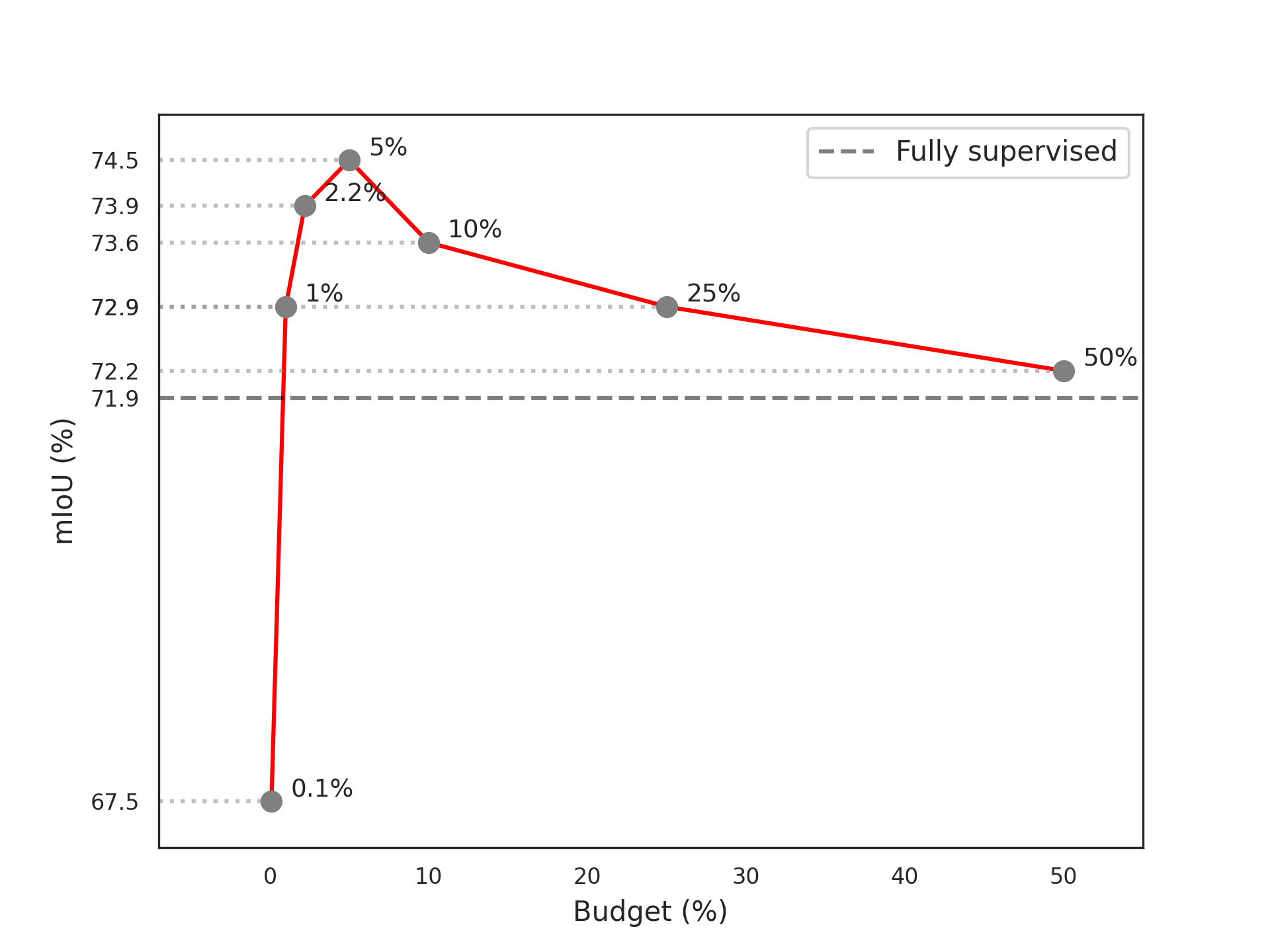
Figure 5: Performance on GTAV $\rightarrow$ Cityscapes with different budgets.

Region- Vs. Pixel-based criteria  Unlike region impurity in Xie et al. (2022a), the hyperbolic radius is a continuous quantity that can be computed for each pixel. We conduct experiments comparing region- and pixel-based acquisition scores. The results demonstrate a small difference between the two approaches (74.1% Vs. 74.5%).

Labeling budget  We experiment with different labeling budgets, observing performance improvements as the number of labeled pixels increases. However, beyond a threshold of 5%, adding more labeled pixels leads to diminishing returns. We believe this may be explained by data unbalance: taking all labels to domain adapt means that most of them belong to a few classes, specifically road, building and vegetation account for 77% of the labels, which may hinder at successive training rounds due to data redundancy. Detailed results are in Figure 5.

Hyperbolic Feature Reweighting (HFR)  HFR improves training stability and enhances performance in the Hyperbolic model. Although the mIoU improvement is modest (+2%), the main advantage is the training robustness, as the Hyperbolic model otherwise struggles to converge. HFR does not benefit the Euclidean model and instead negatively impacts its performance. Additional results in Appendix A.1

7 Conclusions

We have introduced the first hyperbolic neural network technique for active learning, which we have extensively validated as the novel SoA on semantic segmentation under domain shift. We have identified a novel geometric interpretation of the hyperbolic radius, distinct from the established hyperbolic uncertainty and hyperbolic hierarchy, and we have supported the finding with experimental evidence. The novel concept of hyperbolic radius and its successful use as data acquisition strategy in AL are a step forward in understanding hyperbolic neural networks.

Appendix

This appendix provides additional information and insights on the proposed Hyperbolic Active Learning Optimization (HALO) for semantic segmentation under domain shift.

This supplementary material is structured as follows:

A.1: Additional Ablation Studies

presents additional ablation studies on the embedding dimensions and the proposed Hyperbolic Feature Reweighting (HFR) for Euclidean and hyperbolic backbones;

A.2 Limitations

discusses current limitations and recommendations for further research;

A.3 Broader Impact

regards future applications and the fostered progress in the field of Hyperbolic Neural Networks;

A.4 Additional Hyperbolic Formulas

reports additional employed hyperbolic formulas;

A.5 Implementation Details

describes the training details adopted in the experiments;

A.6 Qualitative Results

showcases representative qualitative results of HALO;

A.7 Data Acquisition Strategy: rounds of selections

illustrates examples of pixel labeling selection and the priorities of the data acquisition strategy at each acquisition round.

A.1 Additional Ablation Studies

Results of HFR  Table A1 provides insights into the performance of hyperbolic and Euclidean models with and without Hyperbolic Feature Reweighting (HFR). In the case of HALO, the performance with and without HFR remains the same in the source-only setting. However, when applied to the source+target ADA scenario, HFR leads to an improvement of 1.2%. It should be noted that HFR also stabilizes the training of hyperbolic models. In fact, when not using HFR, training requires a warm-up schedule and, still, it does not converge in approximately 20% of the runs. HFR improves therefore performance for ADA and it is important for hyperbolic learning stability.

Table A1: HFR Performance Comparison: Evaluating the impact of Hyperbolic Feature Reweighting (HFR) on hyperbolic and Euclidean models in source-only and source+target protocols.

Encoder	Protocol	HFR	mIoU (%)
DeepLab-v3+	source-only	✗	36.3
DeepLab-v3+	source-only	✓	22.7
Hyper DeepLab-v3+	source-only	✗	39.0
Hyper DeepLab-v3+	source-only	✓	38.9
HALO	source$+$target	✗	72.5
HALO	source$+$target	✓	74.5

A.2 Limitations

While we have presented experimental evidence supporting the need for a novel interpretation of the hyperbolic radius, our work lacks a rigorous mathematical validation of the properties of the hyperbolic radius within the given experimental setup. Future research should delve into this mathematical aspect to formalize and prove these properties.

HALO’s reliance on a source model pretrained on synthetic data introduces challenges related to large-scale simulation efforts and the need for effective synthetic-to-real domain adaptation. Exploring alternative strategies, such as self-supervised pre-training on real source datasets, could be a promising research direction to mitigate these challenges.

Although Active Domain Adaptation significantly reduces labeling costs, the manual annotation of individual pixels can be a time-consuming task. Further investigation into human-robot interaction methodologies to streamline pixel annotation processes and expedite the annotation workflow is needed.

A.3 Broader Impact

Hyperbolic Neural Networks (HNN) have recently become mainstream, reaching state-of-the-art across several tasks. Still, the theory and interpretation of HNN is diverse across tasks. Specifically, the hyperbolic radius has been interpreted as a continuum hierarchical parent-to-child measure or as an estimate of uncertainty. Our novel third way of interpreting the radius adds to the flourishing framework of HNN, making a step forward.

A.4 Additional Hyperbolic Formulas

Here we report established hyperbolic formulas which have used in the paper, but not shown due to space constraints.

Poincaré Distance Given two hyperbolic vectors x, y $\in\mathbb{D}^{N}_{c}$, the Poincaré distance represents the distance between them in the Poincaré ball and is defined as:

$$d_{Poin}(x,y)=\frac{2}{\sqrt{c}}\ tanh^{-1}(\sqrt{c}\|-x\oplus_{c}y\|)$$ (A1)

where $\oplus_{c}$ is the Möbius addition defined in Eq. 2 of the paper and $c$ is the manifold curvature.

Riemannian Variance Given a set of hyperbolic vectors $x_{1},...,x_{M}\in\mathbb{D}^{N}_{c}$ we define the Riemannian variance between them as:

$$\sigma^{2}=\frac{1}{M}\sum_{i=1}^{M}d_{Poin}^{2}(x_{i},\mu)$$ (A2)

where $\mu$ is the Fréchet mean, the hyperbolic vector that minimizes the Riemannian variance. $\mu$ cannot be computed in closed form, but it may be approximated with a recursive algorithm Lou et al. (2021).

A.5 Implementation details

For all experiments, the model is trained on 4 Tesla V100 GPUs using PyTorch Paszke et al. (2019) and PyTorch Lightning with an effective batch-size of 8 samples (2 per GPU). The DeepLab-v3+ architecture is used with an Imagenet pre-trained ResNet-101 as the backbone. RiemannianSGD optimizer with momentum of $0.9$ and weight decay of $5\times 10^{-4}$ is used for all the trainings. The base learning rates for the encoder and decode head are $1\times 10^{-3}$ and $1\times 10^{-2}$ respectively, and they are decayed with a ”polynomial” schedule with power $0.5$. The models are pre-trained for 15K iterations and adapted for an additional 15K on the target set. As per Xie et al. (2022a), the source images are resized to $1280\times 720$, while the target images are resized to $1280\times 640$.

A.6 Qualitative Results

In Figure 8, we present visualizations of HALO’s predicted segmentation maps and the selected pixels. In the first row, HALO prioritizes the selection of pixels that are not easily interpretable, as evident in the fence or wall on the right side of the image. Notably, HALO does not limit itself to selecting contours exclusively; it continues to acquire pixels within classes if they exhibit high unexplained class complexity (determined by the hyperbolic radius). This behavior is also observed in rows 2, 3, and 4 of Figure 8. For classes with lower complexity, such as road and car, HALO acquires only the contours. However, for more intricate classes like pole and signs, it also selects pixels within the class.

In rows 5, 6, and 8, the images depict a crowded scene with numerous small objects from various classes. Remarkably, the selection process directly targets the more complex classes (such as pole and signs), providing an accurate classification of these. In row 7, we observe an example where the most common classes (road, vegetation, building, sky) dominate the majority of the image. HALO, guided by the concept of unexplained class complexity, efficiently allocates the label budget by focusing on the more complex classes, rather than expending resources on these prevalent ones. Refer to Sec. A.7 and Fig. 7 for a detailed overview of the selection prioritization during each active learning round.

A.7 Data Acquisition Strategy: rounds of selections

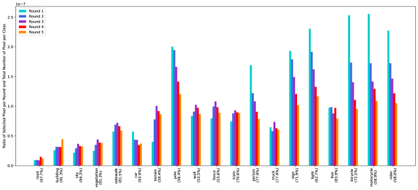
Figure 6: Ratio between the selected pixels for each class at each round and the total number of pixels per class. Each color shows the ratio in the specific round. On the $x$-axis are reported the classes with the relative mIoU (%) of HALO (cf. Table 1 of the main paper) ordered according to they decreasing hyperbolic radius.

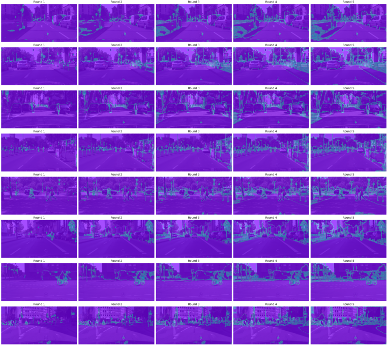
Figure 7: Qualitative analysis on the pixel selected by HALO at each round. Zoom in to see details.

In this section, we analyze how the model prioritizes the selection of the pixels during the different rounds. In Fig. 6, we consider the ratio between the selected pixel at each round and the total number of pixels for the considered class. Note how the model selects in the early stages from the class with high intrinsic difficulty (e.g., rider, bicycle, pole). During the different rounds, the selected pixels decrease because of the scarcity of pixels associated with these classes. On the other hand, the classes with lower unexplained class complexity are less considered in the early stages and the model selects from them in the intermediate rounds if the class has an intermediate complexity (e.g., wall, fence, sidewalk) or in the last stages if the classes have low complexity (e.g., road or building).

The qualitative samples of pixel selections in Fig. 7 corroborate this observation. In rounds 1 and 2, the model gives precedence to selecting pixels from classes exhibiting high ”unexplained class complexity” (e.g., poles, sign, person, or rider). Subsequently, HALO shifts its focus to two distinct objectives: i) acquiring contours from classes with lower complexity (e.g., road, car, or vegetation), and ii) obtaining additional pixels from more complex classes (e.g., pole or wall). Notably, in rows 1, 2, 3, 5, and 6, HALO gives priority to selecting complete objects right from the initial round (as seen with the sign). Another noteworthy instance is the acquisition of the bicycle in row 7. The hyperbolic radius score enables the acquisition of contours that extend beyond the boundaries of pseudo-label classes. In this case, we observe precise delineation of the internal portions of the wheels.

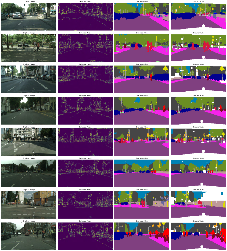
Figure 8: Qualitative Results Visualization for the GTAV $\rightarrow$ Cityscapes Task. The figure showcases different subfigures representing: the original image, HALO’s pixel selection, HALO’s prediction, and the ground-truth label. Zoom in for the details.

References

- Ash et al. (2019) Jordan T Ash, Chicheng Zhang, Akshay Krishnamurthy, John Langford, and Alekh Agarwal. Deep batch active learning by diverse, uncertain gradient lower bounds. arXiv preprint arXiv:1906.03671, 2019.
- Atigh et al. (2022) M. Atigh, J. Schoep, E. Acar, N. Van Noord, and P. Mettes. Hyperbolic image segmentation. In 2022 IEEE/CVF Conference on Computer Vision and Pattern Recognition (CVPR), pp. 4443–4452, Los Alamitos, CA, USA, jun 2022. IEEE Computer Society.
- Ben-David et al. (2010) Shai Ben-David, John Blitzer, Koby Crammer, Alex Kulesza, Fernando Pereira, and Jennifer Vaughan. A theory of learning from different domains. Machine Learning, 79:151–175, 2010.
- Brüggemann et al. (2023) David Brüggemann, Christos Sakaridis, Prune Truong, and Luc Van Gool. Refign: Align and refine for adaptation of semantic segmentation to adverse conditions. In Proceedings of the IEEE/CVF Winter Conference on Applications of Computer Vision, pp. 3174–3184, 2023.
- Chami et al. (2019) Ines Chami, Zhitao Ying, Christopher Ré, and Jure Leskovec. Hyperbolic graph convolutional neural networks. Advances in neural information processing systems, 32, 2019.
- Chami et al. (2020) Ines Chami, Albert Gu, Vaggos Chatziafratis, and Christopher Ré. From trees to continuous embeddings and back: Hyperbolic hierarchical clustering. Advances in Neural Information Processing Systems, 33:15065–15076, 2020.
- Chen et al. (2022) Bike Chen, Wei Peng, Xiaofeng Cao, and Juha Röning. Hyperbolic uncertainty aware semantic segmentation. arXiv preprint arXiv:2203.08881, 2022.
- Chen et al. (2018a) Liang-Chieh Chen, George Papandreou, Iasonas Kokkinos, Kevin Murphy, and Alan L. Yuille. Deeplab: Semantic image segmentation with deep convolutional nets, atrous convolution, and fully connected crfs. IEEE Transactions on Pattern Analysis and Machine Intelligence, 40(4):834–848, Apr 2018a.
- Chen et al. (2018b) Liang-Chieh Chen, Yukun Zhu, George Papandreou, Florian Schroff, and Hartwig Adam. Encoder-decoder with atrous separable convolution for semantic image segmentation. In Computer Vision – ECCV 2018, pp. 833–851, Cham, 2018b.
- Cheng et al. (2021) Yiting Cheng, Fangyun Wei, Jianmin Bao, Dong Chen, Fang Wen, and Wenqiang Zhang. Dual path learning for domain adaptation of semantic segmentation. In Proceedings of the IEEE/CVF International Conference on Computer Vision, pp. 9082–9091, 2021.
- Cordts et al. (2016) Marius Cordts, Mohamed Omran, Sebastian Ramos, Timo Rehfeld, Markus Enzweiler, Rodrigo Benenson, Uwe Franke, Stefan Roth, and Bernt Schiele. The cityscapes dataset for semantic urban scene understanding. CoRR, abs/1604.01685, 2016.
- Ermolov et al. (2022) Aleksandr Ermolov, Leyla Mirvakhabova, Valentin Khrulkov, Nicu Sebe, and Ivan Oseledets. Hyperbolic vision transformers: Combining improvements in metric learning. In Proceedings of the IEEE/CVF Conference on Computer Vision and Pattern Recognition, pp. 7409–7419, 2022.
- Franco et al. (2023) Luca Franco, Paolo Mandica, Bharti Munjal, and Fabio Galasso. Hyperbolic self-paced learning for self-supervised skeleton-based action representations. In The Eleventh International Conference on Learning Representations, 2023.
- French et al. (2017) Geoffrey French, Michal Mackiewicz, and Mark Fisher. Self-ensembling for visual domain adaptation. arXiv preprint arXiv:1706.05208, 2017.
- Fu et al. (2021) Bo Fu, Zhangjie Cao, Jianmin Wang, and Mingsheng Long. Transferable query selection for active domain adaptation. In Proceedings of the IEEE/CVF Conference on Computer Vision and Pattern Recognition, pp. 7272–7281, 2021.
- Gal et al. (2017) Yarin Gal, Riashat Islam, and Zoubin Ghahramani. Deep bayesian active learning with image data. In International conference on machine learning, pp. 1183–1192. PMLR, 2017.
- Ganea et al. (2018) Octavian Ganea, Gary Bécigneul, and Thomas Hofmann. Hyperbolic neural networks. Advances in neural information processing systems, 31, 2018.
- Golestaneh & Kitani (2020) S Alireza Golestaneh and Kris M Kitani. Importance of self-consistency in active learning for semantic segmentation. BMVC, 2020.
- Gulcehre et al. (2018) Caglar Gulcehre, Misha Denil, Mateusz Malinowski, Ali Razavi, Razvan Pascanu, Karl Moritz Hermann, Peter Battaglia, Victor Bapst, David Raposo, Adam Santoro, et al. Hyperbolic attention networks. arXiv preprint arXiv:1805.09786, 2018.
- Guo et al. (2022) Y. Guo, X. Wang, Y. Chen, and S. X. Yu. Clipped hyperbolic classifiers are super-hyperbolic classifiers. In 2022 IEEE/CVF Conference on Computer Vision and Pattern Recognition (CVPR), pp. 1–10, Los Alamitos, CA, USA, jun 2022. IEEE Computer Society.
- Hoffman et al. (2018) Judy Hoffman, Eric Tzeng, Taesung Park, Jun-Yan Zhu, Phillip Isola, Kate Saenko, Alexei Efros, and Trevor Darrell. Cycada: Cycle-consistent adversarial domain adaptation. In International conference on machine learning, pp. 1989–1998. Pmlr, 2018.
- Hoyer et al. (2023) Lukas Hoyer, Dengxin Dai, Haoran Wang, and Luc Van Gool. Mic: Masked image consistency for context-enhanced domain adaptation. In Proceedings of the IEEE/CVF Conference on Computer Vision and Pattern Recognition, pp. 11721–11732, 2023.
- Jiang et al. (2020) Pin Jiang, Aming Wu, Yahong Han, Yunfeng Shao, Meiyu Qi, and Bingshuai Li. Bidirectional adversarial training for semi-supervised domain adaptation. In IJCAI, pp. 934–940, 2020.
- Kirsch et al. (2019) Andreas Kirsch, Joost van Amersfoort, and Yarin Gal. Batchbald: Efficient and diverse batch acquisition for deep bayesian active learning, 2019.
- Kundu et al. (2021) Jogendra Nath Kundu, Akshay Kulkarni, Amit Singh, Varun Jampani, and R. Venkatesh Babu. Generalize then adapt: Source-free domain adaptive semantic segmentation. In Proceedings of the IEEE/CVF International Conference on Computer Vision (ICCV), pp. 7046–7056, October 2021.
- Liu et al. (2019) Qi Liu, Maximilian Nickel, and Douwe Kiela. Hyperbolic graph neural networks. Advances in neural information processing systems, 32, 2019.
- Liu et al. (2021) Yuang Liu, Wei Zhang, and Jun Wang. Source-free domain adaptation for semantic segmentation. In Proceedings of the IEEE/CVF Conference on Computer Vision and Pattern Recognition, pp. 1215–1224, 2021.
- Liu et al. (2020) Ziwei Liu, Zhongqi Miao, Xingang Pan, Xiaohang Zhan, Dahua Lin, Stella X Yu, and Boqing Gong. Open compound domain adaptation. In Proceedings of the IEEE/CVF Conference on Computer Vision and Pattern Recognition, pp. 12406–12415, 2020.
- Lou et al. (2021) Aaron Lou, Isay Katsman, Qingxuan Jiang, Serge Belongie, Ser-Nam Lim, and Christopher De Sa. Differentiating through the fréchet mean, 2021.
- Mei et al. (2020) Ke Mei, Chuang Zhu, Jiaqi Zou, and Shanghang Zhang. Instance adaptive self-training for unsupervised domain adaptation. In Computer Vision–ECCV 2020: 16th European Conference Proceedings, Part XXVI 16, pp. 415–430, 2020.
- Mittal et al. (2023) Sudhanshu Mittal, Joshua Niemeijer, Jörg P. Schäfer, and Thomas Brox. Best practices in active learning for semantic segmentation, 2023.
- Nickel & Kiela (2017) Maximilian Nickel and Douwe Kiela. Poincaré embeddings for learning hierarchical representations, 2017.
- Ning et al. (2021) Munan Ning, Donghuan Lu, Dong Wei, Cheng Bian, Chenglang Yuan, Shuang Yu, Kai Ma, and Yefeng Zheng. Multi-anchor active domain adaptation for semantic segmentation. In Proceedings of the IEEE/CVF International Conference on Computer Vision, pp. 9112–9122, 2021.
- Paszke et al. (2019) Adam Paszke, Sam Gross, Francisco Massa, Adam Lerer, James Bradbury, Gregory Chanan, Trevor Killeen, Zeming Lin, Natalia Gimelshein, Luca Antiga, Alban Desmaison, Andreas Kopf, Edward Yang, Zachary DeVito, Martin Raison, Alykhan Tejani, Sasank Chilamkurthy, Benoit Steiner, Lu Fang, Junjie Bai, and Soumith Chintala. Pytorch: An imperative style, high-performance deep learning library. In Advances in Neural Information Processing Systems 32, pp. 8024–8035. 2019.
- Paul et al. (2020) Sujoy Paul, Yi-Hsuan Tsai, Samuel Schulter, Amit K. Roy-Chowdhury, and Manmohan Chandraker. Domain adaptive semantic segmentation using weak labels, 2020.
- Prabhu et al. (2021) Viraj Prabhu, Arjun Chandrasekaran, Kate Saenko, and Judy Hoffman. Active domain adaptation via clustering uncertainty-weighted embeddings. In Proceedings of the IEEE/CVF International Conference on Computer Vision, pp. 8505–8514, 2021.
- Richter et al. (2016) Stephan R. Richter, Vibhav Vineet, Stefan Roth, and Vladlen Koltun. Playing for data: Ground truth from computer games. In European Conference on Computer Vision (ECCV), volume 9906, pp. 102–118, 2016.
- Ros et al. (2016) German Ros, Laura Sellart, Joanna Materzynska, David Vazquez, and Antonio M. Lopez. The synthia dataset: A large collection of synthetic images for semantic segmentation of urban scenes. In The IEEE Conference on Computer Vision and Pattern Recognition (CVPR), June 2016.
- S & Fleuret (2021) Prabhu Teja S and François Fleuret. Uncertainty reduction for model adaptation in semantic segmentation. In 2021 IEEE/CVF Conference on Computer Vision and Pattern Recognition (CVPR), pp. 9608–9618, 2021.
- Saito et al. (2019) Kuniaki Saito, Donghyun Kim, Stan Sclaroff, Trevor Darrell, and Kate Saenko. Semi-supervised domain adaptation via minimax entropy. In Proceedings of the IEEE/CVF International Conference on Computer Vision (ICCV), October 2019.
- Sakaridis et al. (2021) Christos Sakaridis, Dengxin Dai, and Luc Van Gool. ACDC: The adverse conditions dataset with correspondences for semantic driving scene understanding. In Proceedings of the IEEE/CVF International Conference on Computer Vision (ICCV), October 2021.
- Sala et al. (2018) Frederic Sala, Chris De Sa, Albert Gu, and Christopher Ré. Representation tradeoffs for hyperbolic embeddings. In International conference on machine learning, pp. 4460–4469. PMLR, 2018.
- Sarkar (2012) Rik Sarkar. Low distortion delaunay embedding of trees in hyperbolic plane. In Graph Drawing: 19th International Symposium, GD 2011, Revised Selected Papers 19, pp. 355–366, 2012.
- Sener & Savarese (2017) Ozan Sener and Silvio Savarese. Active learning for convolutional neural networks: A core-set approach. arXiv preprint arXiv:1708.00489, 2017.
- Shimizu et al. (2020) Ryohei Shimizu, Yusuke Mukuta, and Tatsuya Harada. Hyperbolic neural networks++. arXiv preprint arXiv:2006.08210, 2020.
- Shin et al. (2021a) Gyungin Shin, Weidi Xie, and Samuel Albanie. All you need are a few pixels: semantic segmentation with pixelpick. In Proceedings of the IEEE/CVF International Conference on Computer Vision, pp. 1687–1697, 2021a.
- Shin et al. (2020) Inkyu Shin, Sanghyun Woo, Fei Pan, and In So Kweon. Two-phase pseudo label densification for self-training based domain adaptation. In Computer Vision–ECCV 2020: 16th European Conference, Proceedings, Part XIII 16, pp. 532–548, 2020.
- Shin et al. (2021b) Inkyu Shin, Dong-Jin Kim, Jae Won Cho, Sanghyun Woo, Kwanyong Park, and In So Kweon. Labor: Labeling only if required for domain adaptive semantic segmentation. In Proceedings of the IEEE/CVF International Conference on Computer Vision, pp. 8588–8598, 2021b.
- Singh (2021) Ankit Singh. Clda: Contrastive learning for semi-supervised domain adaptation. In M. Ranzato, A. Beygelzimer, Y. Dauphin, P.S. Liang, and J. Wortman Vaughan (eds.), Advances in Neural Information Processing Systems, volume 34, pp. 5089–5101. Curran Associates, Inc., 2021.
- Singh et al. (2021) Anurag Singh, Naren Doraiswamy, Sawa Takamuku, Megh Bhalerao, Titir Dutta, Soma Biswas, Aditya Chepuri, Balasubramanian Vengatesan, and Naotake Natori. Improving semi-supervised domain adaptation using effective target selection and semantics. In 2021 IEEE/CVF Conference on Computer Vision and Pattern Recognition Workshops (CVPRW), pp. 2703–2712, 2021.
- Sinha et al. (2019) Samarth Sinha, Sayna Ebrahimi, and Trevor Darrell. Variational adversarial active learning. In Proceedings of the IEEE/CVF International Conference on Computer Vision, pp. 5972–5981, 2019.
- Su et al. (2020) Jong-Chyi Su, Yi-Hsuan Tsai, Kihyuk Sohn, Buyu Liu, Subhransu Maji, and Manmohan Chandraker. Active adversarial domain adaptation. In Proceedings of the IEEE/CVF Winter Conference on Applications of Computer Vision, pp. 739–748, 2020.
- Surís et al. (2021) Dídac Surís, Ruoshi Liu, and Carl Vondrick. Learning the predictability of the future. In Proceedings of the Conference on Computer Vision and Pattern Recognition, pp. 12607–12617, 2021.
- Tifrea et al. (2018) Alexandru Tifrea, Gary Bécigneul, and Octavian-Eugen Ganea. Poincaré glove: Hyperbolic word embeddings. arXiv preprint arXiv:1810.06546, 2018.
- van Spengler et al. (2023) Max van Spengler, Erwin Berkhout, and Pascal Mettes. Poincaré resnet, 2023.
- Vu et al. (2019) Tuan-Hung Vu, Himalaya Jain, Maxime Bucher, Matthieu Cord, and Patrick Perez. Advent: Adversarial entropy minimization for domain adaptation in semantic segmentation. In Proceedings of the IEEE/CVF Conference on Computer Vision and Pattern Recognition (CVPR), June 2019.
- Wang & Shang (2014) Dan Wang and Yi Shang. A new active labeling method for deep learning. In 2014 International joint conference on neural networks (IJCNN), pp. 112–119. IEEE, 2014.
- Wang et al. (2016) Keze Wang, Dongyu Zhang, Ya Li, Ruimao Zhang, and Liang Lin. Cost-effective active learning for deep image classification. IEEE Transactions on Circuits and Systems for Video Technology, 27(12):2591–2600, 2016.
- Wu et al. (2021) Tsung-Han Wu, Yueh-Cheng Liu, Yu-Kai Huang, Hsin-Ying Lee, Hung-Ting Su, Ping-Chia Huang, and Winston H Hsu. Redal: Region-based and diversity-aware active learning for point cloud semantic segmentation. In Proceedings of the IEEE/CVF International Conference on Computer Vision, pp. 15510–15519, 2021.
- Wu et al. (2022) Tsung-Han Wu, Yi-Syuan Liou, Shao-Ji Yuan, Hsin-Ying Lee, Tung-I Chen, Kuan-Chih Huang, and Winston H Hsu. D 2 ada: Dynamic density-aware active domain adaptation for semantic segmentation. In Computer Vision ECCV 2022 Proceedings, Part XXIX, pp. 449–467. Springer, 2022.
- Xie et al. (2022a) Binhui Xie, Longhui Yuan, Shuang Li, Chi Harold Liu, and Xinjing Cheng. Towards fewer annotations: Active learning via region impurity and prediction uncertainty for domain adaptive semantic segmentation. In Proceedings of the IEEE/CVF Conference on Computer Vision and Pattern Recognition (CVPR), pp. 8068–8078, June 2022a.
- Xie et al. (2022b) Binhui Xie, Longhui Yuan, Shuang Li, Chi Harold Liu, Xinjing Cheng, and Guoren Wang. Active learning for domain adaptation: An energy-based approach. In Proceedings of the AAAI Conference on Artificial Intelligence, volume 36, pp. 8708–8716, 2022b.
- Yang & Soatto (2020) Yanchao Yang and Stefano Soatto. Fda: Fourier domain adaptation for semantic segmentation. In Proceedings of the IEEE/CVF Conference on Computer Vision and Pattern Recognition (CVPR), June 2020.
- You et al. (2021) Fuming You, Jingjing Li, Lei Zhu, Zhi Chen, and Zi Huang. Domain adaptive semantic segmentation without source data. In Proceedings of the 29th ACM International Conference on Multimedia, pp. 3293–3302. Association for Computing Machinery, 2021.
- Zhang et al. (2021) Pan Zhang, Bo Zhang, Ting Zhang, Dong Chen, Yong Wang, and Fang Wen. Prototypical pseudo label denoising and target structure learning for domain adaptive semantic segmentation. In Proceedings of the IEEE/CVF conference on computer vision and pattern recognition, pp. 12414–12424, 2021.
- Zheng & Yang (2021) Zhedong Zheng and Yi Yang. Rectifying pseudo label learning via uncertainty estimation for domain adaptive semantic segmentation. International Journal of Computer Vision, 129(4):1106–1120, 2021.
- Zou et al. (2018) Yang Zou, Zhiding Yu, BVK Vijaya Kumar, and Jinsong Wang. Unsupervised domain adaptation for semantic segmentation via class-balanced self-training. In Proceedings of the European Conference on Computer Vision (ECCV), pp. 289–305, 2018.
- Zou et al. (2019) Yang Zou, Zhiding Yu, Xiaofeng Liu, B.V.K. Vijaya Kumar, and Jinsong Wang. Confidence regularized self-training. In The IEEE International Conference on Computer Vision (ICCV), October 2019.