Pipit: Enabling programmatic analysis of parallel execution traces

Abstract.

Performance analysis is an important part of the oft-repeated, iterative process of performance tuning during the development of parallel programs. Per-process per-thread traces (detailed logs of events with timestamps) enable in-depth analysis of parallel program execution to identify various kinds of performance issues. Often times, trace collection tools provide a graphical tool to analyze the trace output. However, these GUI-based tools only support specific file formats, are difficult to scale when the data is large, limit data exploration to the implemented graphical views, and do not support automated comparisons of two or more datasets. In this paper, we present a programmatic approach to analyzing parallel execution traces by leveraging pandas, a powerful Python-based data analysis library. We have developed a Python library, Pipit, on top of pandas that can read traces in different file formats (OTF2, HPCToolkit, Projections, Nsight, etc.) and provide a uniform data structure in the form of a pandas DataFrame. Pipit provides operations to aggregate, filter, and transform the events in a trace to present the data in different ways. We also provide several functions to quickly identify performance issues in parallel executions.

⬇

1import pipit as ppt

2

3trace = ppt.Trace.from_otf2(’ping-pong’)

4trace.plot_timeline(instant_events=...)

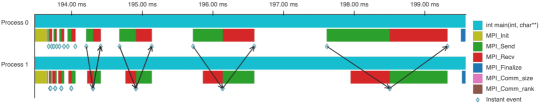
Figure 1. Pipit provides a Python API to read, manipulate, and explore parallel execution traces programmatically (left) and to visualize them (right).

1. Motivation

Software development in high performance computing (HPC) often involves an iterative process of writing code, analyzing performance, making changes to tune performance, and then doing more analysis and tuning. Hence, it is important to optimize the process of performance analysis to reduce developer effort as much as possible. Detailed performance analysis, and specifically tasks such as critical path detection, message dependency analysis, and root cause analysis often require the collection and analysis of parallel execution traces. Execution traces are detailed logs of individual events (compute, communication routines, I/O etc.) with timestamps. Several performance tools such as Score-P (Knüpfer et al., 2012), HPCToolkit (Adhianto et al., 2010), Nsight Systems (NVIDIA, [n. d.]), and Projections (Kale et al., 2006) can collect per-process, per-thread and even per-GPU traces of parallel programs.

Table 1. Capabilities in different graphical trace analysis and visualization tools.

	Events	Metrics	Time	Outlier	Flat	Comm.	Msg Size	Call	Pattern	Manual	Guided
	over time	over time	Profile	Analysis	Profile	Matrix	Histogram	Stack	Detect.	Mult. Run	Mult. Run
Vampir	✓	✓	✓	$\times$	✓	✓	✓	✓	$\times$	✓	$\times$
hpcviewer	✓	$\times$	✓	$\times$	✓	$\times$	$\times$	✓	$\times$	$\times$	$\times$
Projections	✓	✓	✓	✓	$\times$	✓	✓	$\times$	$\times$	✓	$\times$
Nsight	✓	✓	$\times$	✓	✓	$\times$	$\times$	✓	$\times$	✓	$\times$
Perfetto	✓	✓	$\times$	$\times$	✓	$\times$	$\times$	✓	$\times$	$\times$	$\times$
This work	✓	✓	✓	✓	✓	✓	✓	✓	✓	✓	✓

When production scientific applications are run with a large number of processes even for short periods of time, the traces grow in size and complexity quickly due to the large number of events logged per process. This often makes the task of trace analysis unwieldy and challenging. Often, trace collection tools also provide a corresponding graphical tool for analyzing trace data – some popular examples are Vampir (Knüpfer et al., 2008), hpcviewer (Adhianto et al., 2010), and Nsight Systems (NVIDIA, [n. d.]). However, these GUI-based tools have several limitations. First, each tool only supports specific file formats, and end users have to familiarize themselves with the interfaces of multiple tools to analyze different traces effectively. Second, when using GUI-based tools, end users are constrained in their exploration of the data by the views provided by each tool. Moreover, in most graphical tools, repeating the same analysis twice on the same or different datasets is a manual process, with limited support for saving/automating analysis. Third, since parallel traces can be large in two dimensions (time and number of processes/threads), visualizations often have issues with scalability beyond small datasets. Finally, while some graphical tools allow loading trace data from two different executions, the exploration is user-driven and manual, and they do not provide automated comparisons of two or more datasets.

There are several challenges to developing a single tool for trace analysis that solves all of the issues mentioned above. It should be able to handle different file formats for execution traces. It should allow canned and custom exploration of the data by the end user. Further, it should allow ease of automating performance analysis for oft-repeated tasks. And, it should allow comparisons of traces from multiple executions, hopefully in a somewhat automated manner.

In this paper, we fill the above mentioned gaps in performance analysis of parallel execution traces by developing a programmatic API to analyze them. This API provides full access to the trace data to the end user so that they can explore the data programmatically instead of having to use a graphical interface. Since traces essentially represent a time series of events (with categorical and numerical data per event), we leverage pandas (McKinney, 2017), a powerful Python-based data analysis library for analyzing tabular data. We have developed a performance analysis library called Pipit (name anonymized for double-blind review) that can read traces in different file formats (OTF2 (Eschweiler et al., 2012), HPCToolkit (Adhianto et al., 2010), Projections (Kale et al., 2006), Nsight (NVIDIA, [n. d.]), etc.) and provides a uniform data structure in the form of a pandas DataFrame. Pipit exposes a programmatic API to the end user with operations to aggregate, filter, and transform the events in a trace dataset to explore, manipulate, and visualize the data in different ways.

There are several common data exploration/manipulation tasks that end users perform when analyzing parallel traces. Some examples are – analyzing a heat map or matrix of communication between MPI processes, detecting load imbalance across threads or processes, detecting a critical path in the execution, identifying the most time consuming functions etc. We have designed and implemented many of these operations in the Pipit API to reduce end user effort in such performance analysis related tasks. We also present several case studies that demonstrate the utility and capabilities of Pipit.

The paper makes the following important contributions:

• A unified interface to read traces generated in different formats by different trace measurement tools.

• An open-source library, Pipit, that provides a Programmatic interface to perform common performance analysis tasks using implemented functions.

• Basic visualization support with tens of views to complement the Pipit API in assisting with performance analysis.

• Demonstration of the utility of Pipit in identifying performance issues in several HPC applications.

2. Background and Related Work

A parallel execution trace of a process or thread is essentially time series data, and includes individual events (representing functions, loops, and potentially other code blocks) and their start and end timestamps, along with other optional metrics such as hardware counters. A trace for a parallel program contains this information for multiple processes or threads or both executing within a program execution.

There are many popular trace collection tools such as Score-P (Knüpfer et al., 2012), HPCToolkit (Adhianto et al., 2010), TAU (Shende and Malony, 2006), Nsight systems (NVIDIA, [n. d.]), and Projections (Kale et al., 2006). Score-P, TAU, and HPCToolkit are general purpose tracing tools, which can collect trace data for any C/C++/Fortran program. Nsight and Projections, however, are more specialized for certain parallel programs. Nsight can be used for CUDA-enabled programs running on NVIDIA GPUs, and Projections can be used for Charm++ programs.

2.1. Overview of Trace Visualization Tools

The tracing tools mention above are developed by different research groups, and they use different file formats and serialization techniques to store the parallel trace data. They also have their own complimentary visualization tool to be able to view the traces. Score-P generates traces in the OTF2 open trace format, which can be visualized using Vampir (Knüpfer et al., 2008), and ParaProf (Bell et al., 2003). HPCToolkit produces custom database files that are viewable with hpcviewer. Nsight produces proprietary .qdrep files, viewable with Nsight Graphics. The projections tracing library in Charm++ (Kale and Bhatele, 2013) produces custom log files viewable with a graphical tool, also called Projections.

Before starting the development of Pipit, we conducted a survey of existing trace analysis/visualization tools, and their strengths and weaknesses. Table 1 provides a summary of our study. For each tool in consideration, we evaluated if a certain graphical view that represents a certain kind of analysis of trace data was available or not. Below, we provide a high-level overview of each of the tools we considered.

Vampir is a closed-source GUI-based framework that can be used to to visualize and analyze traces in the OTF2 format. The user interface is comprised of a variety of charts, each designed to process and display a different aspect of the trace. The charts are grouped into three categories: timeline charts, which show events and metrics over time; statistical charts, which display aggregated information about functions, communication, processes, and I/O; and informational charts, which show additional details such as the chart legend and the currently selected item. The tool also offers some filtering capabilities so that users can view charts for certain regions of interest. Finally, Vampir allows opening multiple traces at once and viewing their respective charts side-by-side, enabling manual comparison.

Hpcviewer, used for reading traces generated by HPCToolkit, provides a fairly simple graphical user interface. Hpcviewer provides two main view tabs for analyzing the trace data: a profile view tab and a trace view tab. Hpcviewer’s profile view tab provides three distinct views of the calling context tree aggregated over time and processes: a top-down view, a a bottom-up view and a flat view (similar to gprof’s flat profile). The three views allow users to create derived metrics and filter by any available metrics. Additionally, the top down view also allows users to filter based on the node, rank, and thread. The trace view tab provides five more views for the trace data: the timeline view, the call stack, statistics, depth view, and summary view. The user can also subselect a part of the timeline to zoom in.

Nsight Systems, is a performance analysis tool developed by NVIDIA for CUDA-enabled programs. It supports profiling and tracing, as well as visualization tools to analyze the output. The available views include a timeline view that provides a graphical overview of the events that occurred during the execution of the application. It also provides a top-down view, bottom-up view, and flat view similar to that of hpcviewer which can be filtered by process, functions, etc. These allow the user to analyze the calling contexts of the call sites. Nsight Systems can also generate various different trace and summary reports as part of the stats system view. Finally, Nsight Systems also empowers the user to manually view and inspect multiple datasets at once.

Projections, is the name of both a library to gather performance data of Charm++ programs, and a graphical tool for analyzing summary reports and traces generated by the former. The Projections visualization tool supports several views such as timeline, time profile, and various histograms for communication data and outlier analysis. It is limited to analyzing traces generated from programs written using Charm++, a task-based programming model and runtime. However, it can provide object-specific information about tasks in a Charm++ program.

Perfetto (per, 2022) is a collection of tools used for both collecting and analyzing traces. It is the successor to Chrome’s built-in tracing tool, which featured a front-end visualization interface called Trace Viewer. While Trace Viewer was developed for analyzing the Chrome browser itself, its ease-of-use has prompted developers in different domains, including HPC developers, to use it for general trace visualization. The newer Perfetto supports more trace formats, including a native Protobuf format and the Linux Ftrace format. Its front-end consists of four primary views: an interactive timeline view, customizable pivot tables (containing data aggregates), a SQL engine for querying and processing trace data, and a set of templates for computing metrics and summaries using the SQL engine.

2.2. Other Related Analysis Tools

Other analysis tools have been developed that provide a command line or scripting interface. Extra-P (Calotoiu et al., 2013) provides GUI and a command line interface that can be used for identifying scalability bugs. Similarly, Scalasca (Geimer et al., 2010), a toolset that leverages Score-P for performance measurement and Cube (Saviankou et al., 2015) for performance analysis provides command line interface in addition to its GUI. In addition to its command line interface, Cube also enables users to develop plugins for the GUI. Another performance analysis tool, Hatchet (Bhatele et al., 2019), provides a Python interface that enables programmatic analysis. However, it only supports aggregate profiles and not detailed execution traces.

3. The Pipit Library

We present Pipit, a Python-based library for analyzing parallel execution traces programmatically. Our goals in developing this library were the following: (1) Support several file formats in which execution traces are collected to provide users with a unified interface that works with outputs of many different tracing tools. (2) Provide a programmatic API, which allows users to write simple code for trace analysis and provides several benefits such as flexibility of exploration, scalability, reproducibility, and automation/saving of workflows. And (3) Automate certain common performance analysis tasks for analyzing single and multiple executions. We now describe the considerations in designing and implementing Pipit.

3.1. The trace as a pandas DataFrame

As described in Section 2, a trace contains events with time stamps per process and thread for a parallel program. This data is inherently high-dimensional because we have (events, timestamps) $\times$ (processes, threads, GPUs) $\times$ (performance metrics). We determined that we can treat this data as two-dimensional if we consider event $\times$ timestamp $\times$ process ID (rank) as one axis and all the data collected per event, both numeric and categorical as the other axis. This allows use to use pandas DataFrames as the primary data structure for organizing trace data. A pandas DataFrame is a two-dimensional tabular data structure that allows storing both heterogeneous and sparse data.

Pipit reads an execution trace into a Trace object, which contains an events DataFrame that stores the actual data in a trace. The left gray box in Figure 2 shows a portion of a sample 2-process input trace in CSV format. Most tools record functions as a pair of events (Enter and Leave) – one representing the start of a function and the other the end of the function. Each row has a timestamp for when that event was recorded on a given process. The image to the right of it shows the corresponding events DataFrame created by Pipit. The Python code used to generate a Trace object, foo_bar from an input CSV file is shown at the bottom.

⬇

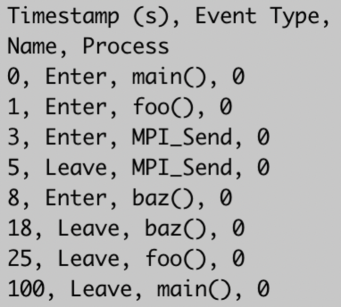
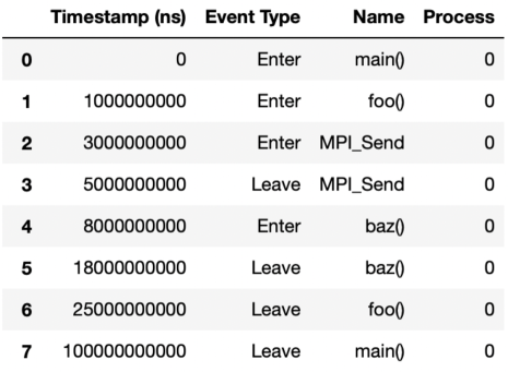
1import pipit as ppt

2

3foo_bar = ppt.Trace.from_csv(’foo-bar.csv’)

4display(foo_bar.events)

Figure 2. A sample trace file in CSV format (left), and the corresponding events DataFrame generated by Pipit after reading it (right) using the code snippet at the bottom.

3.2. Generating a call graph

Calling contexts can be useful to identify the root causes of performance issues. While some tracing tools such as HPCToolkit explicitly record the call stack for each function call, most tools do not. However, by virtue of having timestamps for each function call, we can use the nesting of these calls to extract caller-callee relationships from the data. We use this information to reconstruct the calling context or call stack for each function call. Given the call stack for each event in the trace, we have several options on how to organize this data. If we create a prefix tree from all the call stacks, we can generate a call context tree at every instant in time and for every process or thread. However, this data would grow extremely quickly for complex applications running on large numbers of processes. As a result, we made a decision to aggregate the call graph along two dimensions – over time and across all the processes and threads. We keep this call graph in tree data structure that is a union of all the call graphs in these two dimensions.

3.3. Reading a dataset

One of the main considerations in developing Pipit was to support various file formats that represent different tracing tools. In order to do this, we implemented readers for various file formats. In some cases, we were able to use Python libraries provided by some tools for reading their data. We currently support OTF2 traces, HPCToolkit traces, Projections logs, and Nsight data. When Pipit reads a trace in one of these file formats, it returns a Trace object with an events DataFrame. In some cases, it also contains a definitions DataFrame that has various dictionaries that contain metadata information.

4. The Pipit API

We now describe various operations supported by Pipit that enable the end user to dissect trace data in various ways. We also provide some support for some visualizations that can be used in a Jupyter notebook to compliment our programmatic API (more details in Section 5). However, it should be noted that the main strength of Pipit is the ability to analyze traces programmatically. Various operations in the Pipit API are meant to assist the end user in performance analysis by making it easier, quicker, and automated to a certain degree.

As mentioned in Section 2, we studied the capabilities of GUI-based tools to better understand the common performance analysis tasks performed by HPC users. Below, we provide details of various functions that have been implemented in the Pipit API to enable similar analysis by simply making Python function calls on the Trace object.

4.1. Extracting calling relationships

Raw traces are organized in the form of enter, leave or instant events and their timestamps. We need to traverse and manipulate the DataFrame in the Trace object to match rows that represent the start and end of a function or to identify parent-child relationships using the nesting of events. These functions are necessary in order to start making sense of trace data in terms of user functions and their calling contexts. These functions are described below.

_match_events As mentioned in Section 3, the start and end of a function are typically represented by two separate events, one of type Enter and the other of type Leave. As a result, in the Trace DataFrame, each function invocation appears in two rows with separate timestamps. The Enter row marks the beginning of the function’s execution and the leave row marks the end, always occurring in pairs. In order to calculate the time spent in a function and its children (the function called it), we need to match corresponding enter and leave rows for each function invocation.

Th _match_events function matches the enter and leave rows of each function invocation by adding two columns in the DataFrame that store the row index and timestamp of the corresponding enter or leave. This is done per process and per thread in the case of a parallel trace. To identify matching enter/leave rows, we iterate over the rows in the DataFrame, and every time an enter row is encountered, we pushes its row index and timestamp to a stack. Every time a leave row is encountered, we pops the top of the stack, which is the matching enter row index and timestamp for these leave row. These are added to the the appropriate rows in the DataFrame to form two new columns.

_match_caller_callee The calling stack or calling context of a function invocation can be extremely useful in context-aware performance analysis. It can be helpful for the user to see which call paths are responsible for most of of the performance issues in the application. These relationships are also necessary for calculating the exclusive time spent in each function (time spent in a function minus the time spent in all its descendants/callees in the calling context tree). The _match_caller_callee identifies parent child relationships by traversing the DataFrame and creating three new columns in the DataFrame: row index of a function invocation’s parent, list of row indices of all its children, and its depth in the calling context tree.

Similar to _match_events, the DataFrame is filtered to enter/leave events for the current process and thread being iterated over. Using a stack of DataFrame indices, it keeps track of the parent index. For enter rows, it peeks the stack to get the parent index which is used to modify the current event’s parent and the parent’s children. The current depth in the call tree is also incremented. When a leave row is encountered, an element is popped from the stack and the current depth is decremented. Three new lists are added to the DataFrame to store this data, which allows for additional high-level operations to be performed with them.

_create_cct As discussed in Section 3, when Pipit reads in a trace, it creates a calling context tree (CCT) aggregated over time, threads and processes. The CCT is stored as a separate object in the Trace object. Each event in the DataFrame corresponds to some node in the CCT and stores a reference to that node. Similar to the _match_caller_callee, the _create_cct traverses the entire DataFrame but in this case, computes the call stack for each function invocation, and adds nodes for every function in the call stack to the CCT object. The CCT is updated on the fly as we go through the DataFrame. The CCT is generated by default in all of the data readers before the Trace object is created. Since there is a unified CCT across processes and threads, it can be used to analyze discrepancies in same call paths across different processes and help uncover any related performance issues.

4.2. Analyzing overall performance

Next, we discuss API functions that help analyze the time spent in different parts of the code.

calc_inc_metrics and calc_exc_metrics We need to know the inclusive and exclusive time and other metrics associated with each function invocation prior to commencing any performance analysis. Since the events DataFrame originally contains records of timestamps and other hardware counter readings for Enter/Leave of each function invocation, we need to derive the inclusive and exclusive values for each metric (including execution time). The calc_inc_metrics and calc_exc_metrics functions use _match_events to match indices of enter and leave rows. Once events are matched, corresponding pairs of events can be used to calculate the inclusive metrics associated with each function and the parent-child relationships obtained from _match_caller_callee can be used to subtract the children’s metrics to get the exclusive metrics.

flat_profile A flat profile is often used to get a high-level overview of the most time consuming functions in an execution. Once we calculate the inclusive and exclusive metrics per function invocation, we can use the power of pandas and operations such as groupby to easily calculate the total time spent in each function. We can use the output of this function to focus on a subset of functions in downstream tasks.

time_profile Manually inspecting a timeline of a program execution with a large number of events and processes is a scalability challenge. Instead, we can look at the activity or utilization of all the processes over time. We call this a time profile, which provides a succinct view of the total time spent in different functions across all processes. The time period in the trace is divided into bins, and for each bin, the time_profile function computes the total amount of time spent in different functions (added across all threads and processes). One can think of this as a flat profile over time.

4.3. Analyzing communication performance

Communication is often a scalability bottleneck in MPI programs. Below, we discuss various communication related functionality available in Pipit.

comm_matrix This function computes the data exchanged between pairs of processes and outputs that information as a two-dimensional (2D) numpy array. Note that this information is not available in all trace formats. It requires that each send and receive event have the destination and source process respectively, and the size of the message exchanged. The user can choose to analyze the total number of messages or total volume of communication between each process pair. Analyzing the communication matrix can be challenging when there are a large number of processes. The next few functions compute aggregated communication statistics.

message_size_histogram returns a distribution of the sizes of all messages encountered in the trace. This can help answer questions such as – are there a large number of small messages, or low numbers of large messages.

comm_by_process We can also analyze the amount of communication data sent and received by each process irrespective of the receiver and sender respectively. Similar to comm_matrix, we can choose to look at number of messages or communication volume.

comm_over_time The previous operations generate statistics for communication that are aggregated over time. However, since we have a trace over time, we can also analyze the messaging behavior of programs over time. The comm_over_time operation can calculate both the number of messages, and the total message volume, sent over different time bins.

4.4. Identifying performance issues

Next, we now discuss some advanced operations that attempt to simplify the identification of performance issues.

load_imbalance When parallelizing an application over a large number of MPI processes, load imbalance across processes can lead to worse performance and limit the highest speedup possible by using more cores. To help analyze this in a quick and easy fashion, Pipit provides the user with a load_imbalance function that takes as input a single metric such as exclusive time and the number of processes to output per function that have the highest “load” for that metric. The list of ranks and the imbalance (maximum time across all processes / mean time per process) are provided per function, which makes it easy for the user to identify which functions are especially critical for relieving scaling bottlenecks.

idle_time Processes in a parallel program often wait for messages to arrive, either in a blocking MPI_Recv or MPI_Wait operation. This can be referred to as idle time and can indicate a number of performance issues such as load imbalance, network congestion is system noise (OS jitter). Reducing idle time can improve the scaling of parallel applications. The idle_time operation returns a pandas DataFrame containing the idle times per process. This DataFrame can be sorted by idle time to identify the most or least idle processes.

outlier_detection We also provides an outlier_detection operation that builds upon the idle_time function. Using idle_time to calculate the idle time per process, outlier_detection sorts the resulting DataFrame and returns two lists as a tuple. The first list contains the top $k$ ranks which spent the most time idling, while the second list contains the bottom $k$ ranks which spent the least time idling.

pattern_detection One of the most challenging aspects of trace analysis is identifying a portion of the trace to focus on. Automatic pattern detection can help us find repeating patterns which can either signal performance issues or help us find the start and end of a loop in an iterative program. Such pattern detection can be used to filter a portion of the time series and focus on that for visualization or other downstream tasks. However, detecting patterns is a challenging task if attempted manually. To simplify this task, Pipit provides the pattern_detection function. We utilize the STUMPY library (Law, 2019), which can detect similar repeated subsequences in time series data using matrix profiles (Yeh et al., 2016).

The pattern_detection operation takes a window size (i.e. length of a subsequence), the number of iterations, and a metric as inputs. This function creates a time series by using all the events of one process. Then, it passes this data to the stump function in the STUMPY library, which calculates a matrix profile given a time series and a window size. Then, we pass the matrix profile to the motifs function in the STUMPY library. The motifs function requires setting the number of motifs (i.e. the number of most similar subsequences) expected to be in the data. We use the number of iterations for which the traces were collected for this. Then, we use the indices of these motifs and identify the timestamps at which they occur. We filter out the events that happen outside of these timestamps and output a new DataFrame that contains only the pattern along with the starting indices of the other subsequences identified as motifs.

Since the user has to set the number of iterations and window size, we do not claim that this function fully automates pattern detection. However, it significantly simplifies the task by enabling detecting and analyzing patterns using a few lines of Python code.

multi_run_analysis Another difficult challenge in performance analysis is the comparison of traces from multiple executions. For example, a user might be interested in analyzing how their application scales with different numbers of processes. We provide a simple multi_run_analysis function that takes multiple trace datasets as input and computes flat profiles for each of them given a metric. If the datasets were gathered on different numbers of processes, the output DataFrame, which is indexed by the different setups can help compare performance of different functions across the runs.

4.5. Data Reduction

Finally, Pipit also supports filtering the DataFrame by different parameters to reduce the amount of data to analyze at a time. A user might be interested in analyzing the traces for a subset of processes or for a time period smaller than the entire execution.

filter The filter operation allows users to filter the trace events by different features such as name, timestamp, and process. Users can also instantiate Filter objects, and apply the $not$, $and$, and $or$ logical operators to create compound filters for specific cases. The operation returns a new Trace object containing a reduced events DataFrame. Any of Pipit’s analysis and plotting functions can be applied to the reduced trace.

5. Visualization Support

While Pipit has been primarily designed as a Python library for programmatic analysis, we also provide a basic visual interface to complement the Pipit API. These plotting operations or “views” in Pipit can be used for both exploratory, as well as explanatory, analyses of traces. They have been designed to be fast and scalable for medium-sized traces, while supporting natural user interactions such as hovering, panning, and zooming. The interactive views are generated using Bokeh, a visualization library based on Python and JavaScript. They can be displayed in a Jupyter notebook output cell or a new browser tab, and can be exported as images.

plot_timeline displays the events in a trace over time (see Figure 1). Instant events are represented as diamonds, where its $x$-position represents the event’s timestamp. Function invocations are represented as horizontal boxes, where the left and right $x$-positions represent the start and end of the function. Each process is shown at a unique $y$-position. Finally, MPI messages are represented as arrows pointing from a send event to the corresponding receive event. To avoid visual clutter, these arrows are drawn only when the user clicks on a send or receive event.

Trace files can be extremely large and may contain hundreds of thousands or millions of events. In order to scale the view to accommodate large traces, we split the events into two groups depending on their execution time. The first group of events, consisting of large events, are directly plotted as interactive glyphs. The remaining events, which consist of tiny functions and clusters, are rasterized into an image. Pipit then overlays these individual glyphs and images into one plot, which is then displayed. This splitting and rasterization process happens in real-time as the user interacts, so that individual glyphs will “load in” as the user zooms in to a particular region of interest. This way, Pipit can generate a meaningful visual representation of millions of events instantly on even an entry-level laptop.

plot_time_profile provides a view for the output of the time_profile operation described in Section 4. The stacked bars are color-coded by the function name, and their heights represent the exclusive time spent in each function in each bin. Figure 10 shows a sample time profile for a Kripke execution on 32 processes (region of interest is on the right).

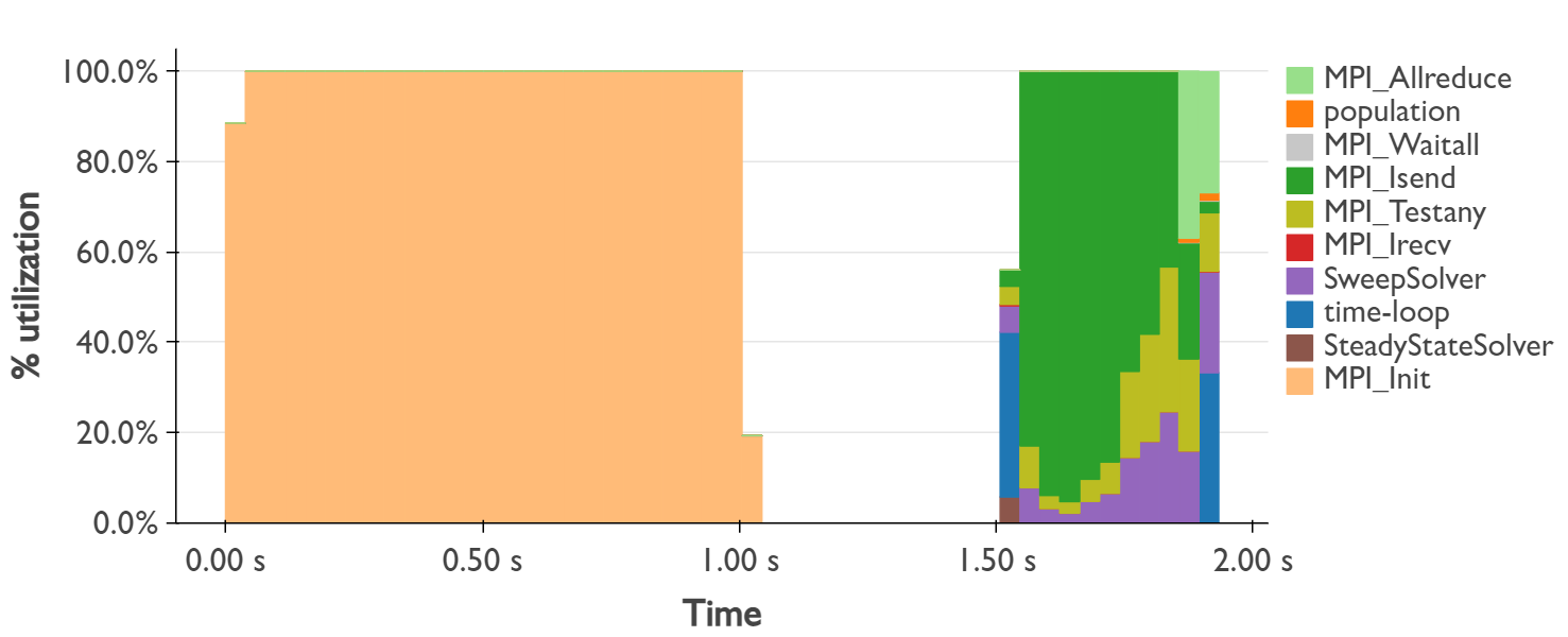
Figure 3. Time profile view of a Kripke execution on 32 processes. On the right, we can see significant time spent in MPI_Isend and SweepSolver.

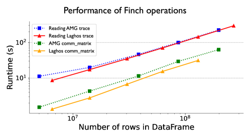
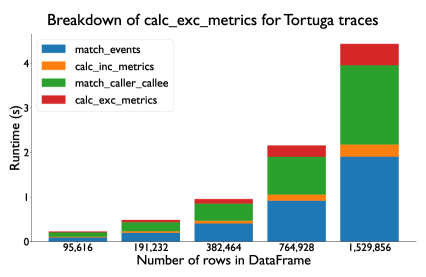
Figure 4. Performance of the OTF2 Reader and comm_matrix function for various traces of AMG and Laghos (left). We compare the runtimes with the number of rows in the corresponding events DataFrame. On the right – Breakdown of time spent in various functions called within calc_exc_metrics when analyzing Tortuga traces.

plot_comm_matrix visualizes the output of the comm_matrix operation, as either a heatmap or a scatter plot. If the heatmap option is specified, the plot displays an image that encodes communication volume as color intensity. On the other hand, if the scatterplot option is specified, the plot displays circles whose areas denote the communication volume.

plot_message_size_histogram displays the output of the message_size_histogram operation as a bar graph, where the heights of the bars represent the frequency of messages for each size bin.

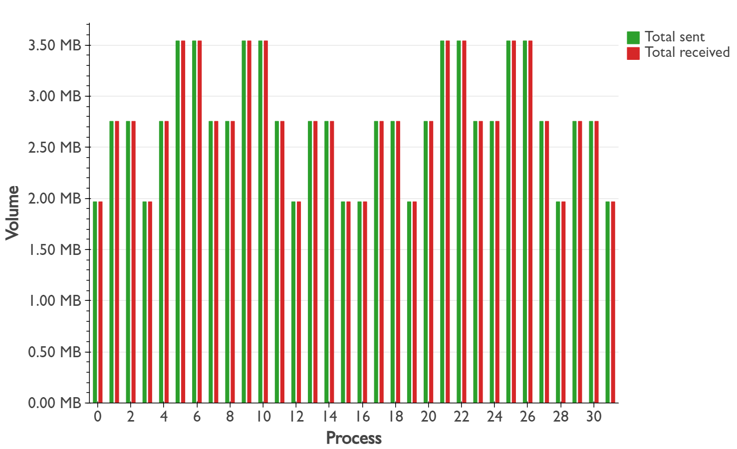
Figure 5. Communication summary view of a Kripke execution on 32 processes. We observe that each process can be placed in one of three sets by its communication volume.

plot_comm_summary visualizes the output of the comm_summary operation as a bar graph, where the heights of the bars represent the total message volume sent and received by each process. Figure 5 shows this view for a Kripke execution on 32 processes.

plot_comm_over_time displays the output of the comm_over_time operation as a bar graph, where the heights of the bars represent the total message volume sent over time.

6. Performance of Pipit Operations

In this section, we present the performance of a few hand-picked Pipit operations to understand their scalability. We have parallelized the reading of input traces in certain file formats using Python multi-processing. Figure 6 shows the time spent by the Pipit OTF2 reader in reading traces of two different applications, AMG (128 processes) and Laghos (256 processes). All the experiments in this section were performed on a single node of an HPC cluster with a dual 64-core AMD EPYC 7763 processor (2.45 GHz base, 3.5 GHz turbo). The OTF2 reader performance scales well with the number of cores, and we get significant speedups from using 64 cores. We plan to gradually parallelize most readers and operations in Pipit.

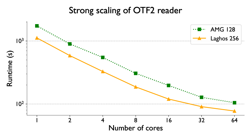
Figure 6. Strong scaling performance of the OTF2 Reader for AMG 128 and Laghos 256 traces.

Next, we analyze the scalability of various Pipit operations w.r.t. increasing trace sizes. For each experiment, we average the times over 3 trials. Figure 4 (left) shows the time spent in the OTF2 reader and the comm_matrix function when reading AMG and Laghos traces of different sizes. We can see that there is a linear relationship between the number of rows in the DataFrame and the runtime.

After a trace is read, most analysis workflows begin with calculating inclusive and exclusive metrics for each function. Hence, we measure the performance of the calc_exc_metrics function and its breakdown into three other functions it invokes: _match_events, calc_inc_metrics, and _match_caller_callee. Figure 4 (right) shows that _match_events and _match_caller_callee take a bulk of the runtime as they iterate over the entire trace. Furthermore, the proportions of time taken by each function remains relatively constant even as the size of the trace increases, showing that these API functions can be used in an efficient and scalable manner.

7. Case Studies

In this section, we demonstrate the power of the Pipit API and the associated visualizations in making performance analysis of parallel applications easier. We use execution traces of a variety of applications, including AMG (Henson and Yang, 2002), Laghos (Dobrev et al., 2012), Kripke (Kunen et al., 2015), Tortuga (a CFD code), and Loimos (a Charm++-based epidemiology simulator).

7.1. Analyzing Communication Performance

We begin with using the communication-related operations in Pipit described in Section 4. In several cases, we demonstrate the results using the visualization support described in Section 5 but this is not required. Users of Pipit can use the programmatic API alone to perform most of the analysis described here. The visual plots are simply a convenient mechanism for presenting the analyses in a research publication.

Figure 7 shows the communication matrix of a Laghos execution on 32 processes, using both a linear colormap (on the left), and a logarithmic colormap (on the right). The code snippet required to generate the views is shown in the listing at the bottom. The heatmap shows the total data exchanged between any two processes. We observe that the matrix is symmetric, and the communication happens along diagonals. This typically suggests a near-neighbor communication pattern in an n-dimensional virtual topology. Switching to logarithmic scale for the colormap makes additional patterns visible in the data.

⬇

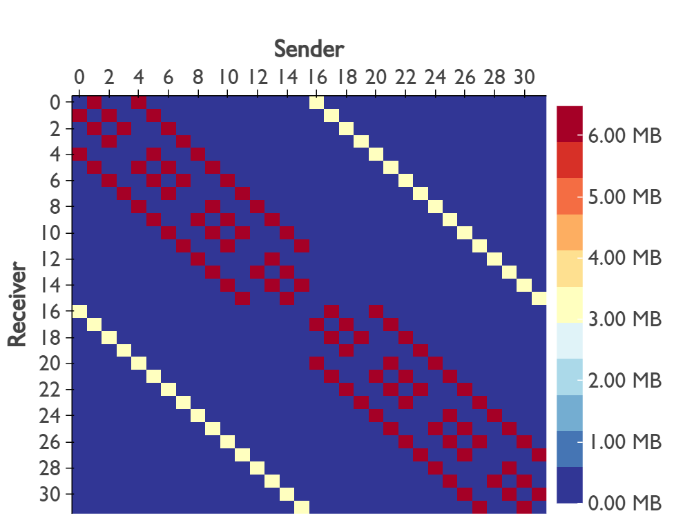
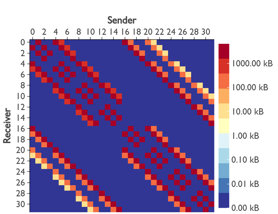
1laghos_32 = pipit.Trace.from_otf2(’./laghos_32’)

2

3laghos_32.plot_comm_matrix(mapping=’linear’)

4laghos_32.plot_comm_matrix(mapping=’log’)

Figure 7. Communication matrix of a Laghos execution on 32 processes, with a linear colormap (left) and logarithmic colormap (right).

Next, we look at the message size histogram of the same Laghos execution in Figure 8. The operation returns the message count in each bin, as well as the edges of the bins of the histogram. In this execution, we see that the sizes of MPI messages are not distributed uniformly. They are clustered into three categories: small messages (between 0 and 1,350 bytes), medium messages (between 5,400-6,750 bytes), and large messages (12,150 - 13,500 bytes).

⬇

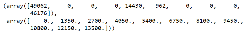
1laghos_32.message_histogram()

Figure 8. Message size histogram of a LAGHOS execution on 32 processes

⬇

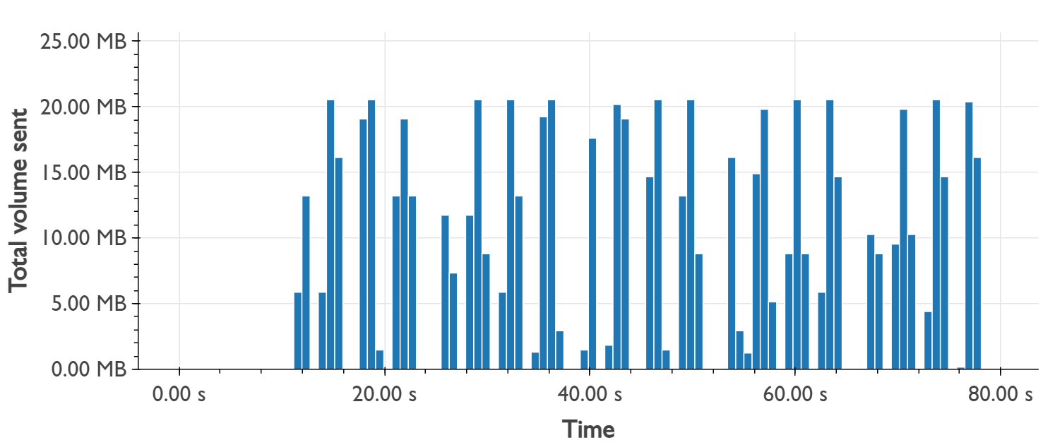
1laghos_32.plot_comm_over_time()

Figure 9. Communication over time of a LAGHOS execution on 32 processes

Finally, to understand how communication changes over time during program execution, we can use the comm_over_time operation, as shown in Figure 9. We see that communication begins at around 12 seconds. The communication volume spikes during certain time intervals, while remaining at zero during others.

7.2. Analyzing Overall Performance

7.2.1. Utilization over time

The time_profile function provides an overview of the activity or utilization over time, and allows the user to identify repeating patterns or functions that might be a significant portion of the total time. In Figure 10, we show a time profile of a CFD code, Tortuga, running on 64 processes. The stacked bar chart allows the user to see what functions are taking up the most amount of time in a specific bin. Focusing on the middle of the time profile, we observe that the computeRhs function (in brown) makes up a significant portion of the total time. We can see that advanceTimestep_Rk3 and spectralRadius have a pattern and are called periodically in the middle region. The code at the bottom shows that using two lines of Python code, a user can glean significant information from a time profile.

⬇

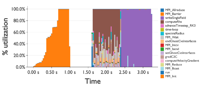
1tortuga_64 = pipit.Trace.from_otf2("tortuga_64")

2tortuga_64.plot_time_profile(num_bins=100, normalized=True)

Figure 10. Time profile of a Tortuga trace with 64 processes.

7.2.2. Pattern detection

To identify patterns in a trace, we use a Score-P user annotated Tortuga execution on 16 processes and set the number of iterations to three when running the program. We pass the number of iterations and a window size (calculated by inspecting the start of each loop iteration) to the pattern_detection function. The top plot in Figure 11 presents a time series generated using the exclusive time values of each enter event in the trace. The bottom plot shows the corresponding matrix profile. The lowest points in the matrix profile indicate similar subsequences (vertical dashed lines). For details about the matrix profiles, we refer the reader to the paper by Yeh et al. (Yeh et al., 2016). As we can see, Pipit can detect patterns using this approach and identify the start of iterations.

⬇

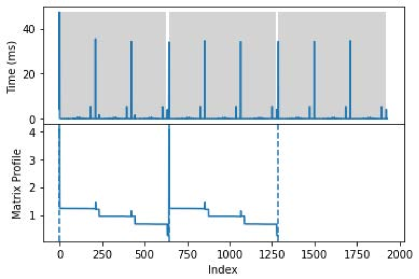
1tortuga_16 = pipit.Trace.from_otf2(’./tortuga_16’)

2matches = tortuga_16.detect_pattern(window_size, iterations, metric=’time.exc’)

3tortuga_16.plot_timeline()

Figure 11. Detecting patterns in a trace. The y-axis in the top plot shows the exclusive time values for each enter event of a process. The grey boxes represents the patterns detected. The vertical dashed lines on the bottom plot (minimum values on the matrix profile) point to start indices of the similar subsequences.

The ability to detect patterns and identify start and end of loop iterations can be extremely useful. When traces get large, and visualizing them in a timeline becomes challenging, we can use the start and end of loop iterations to filter the trace and visualize a smaller time range. We demonstrate this in Section 7.4.

7.3. Finding performance issues

7.3.1. Load imbalance analysis

Using the load_imbalance function, we can expose asymmetry in aggregated runtimes of functions across processes. The code in Figure 12 demonstrates such an example, where a Projections trace of Loimos, an epidemic simulation framework, is read. After this, with just a few lines of code, the output of the load_imbalance function is filtered by the five most time consuming functions to identify the imbalance in them.

⬇

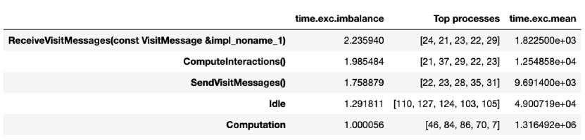
1loimos_128 = pipit.Trace.from_projections(’loimos_128’)

2

3loimos_128.calc_exc_metrics()

4imbalance_df = loimos_128.load_imbalance(num_processes=5)

5imbalance_df = imbalance_df.iloc[0:5].sort_values(by=’time.exc.imbalance’, ascending=False)

Figure 12. Analyzing Load Imbalance for the 5 Most Time Consuming Functions

We notice some interesting observations in the DataFrame output by the load_imbalance operation. First, computeInteractions(), which determines which individuals get infected, is the most time consuming function. It also appears to have high load imbalance, second only to ReceiveVisitMessages(), which is a message processing function. Another interesting observation is that the most overloaded processes are common across the top three functions (21, 22, 23, 29). On the other hand, idle time, which is also significant is largest on a completely non-overlapping set of processes. This could be due to how the application partitions individuals or geographical locations, suggesting that there is some scope for optimization there.

7.3.2. Idle time analysis

We use a 64-process Loimos trace and a 32-process Kripke trace to highlight the utility of the idle_time function in Pipit. Idle_time allows users to quickly and easily identify which processes are waiting for others and are the most idle while which other processes are always busy. Figure 14 shows the code for calculating idle time for the Loimos trace, and the output of the operation for both Loimos (top left) and Kripke (top right). The dataframes show processes sorted from most idle time to least idle time.

⬇

1sizes = [16, 32, 64, 128, 256]

2traces = [pipit.Trace.from_otf2(’./tortuga-’ + str(size)) for size in sizes]

3multirun_df = pipit.Trace.multirun_analysis(traces)

Figure 13. First five columns of the DataFrame returned by the multirun_analysis function for Tortuga traces (left), and plotting this DataFrame as a stacked bar chart (right)

⬇

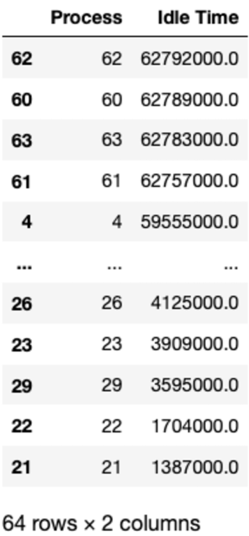
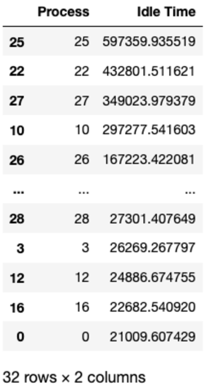
1loimos_64 = pipit.Trace.from_projections(’./loimos_64’)

2

3idle_times = loimos_64.idle_time()

4idle_times = idle_times.sort_values(by=[’Idle Time’], ascending=False)

5display(idle_times)

Figure 14. Idle time computation for Loimos and Kripke.

Similar to pattern_detection, the output of idle time can be used to filter the trace by specific ranks, and then visualize a subset of ranks in the timeline. We demonstrate this in Section 7.4.

7.3.3. Multi-run analysis

We can use the multi_run_analysis function to identify which functions scale poorly as we run on more processes. Such analysis is painstakingly difficult to do with traditional GUI-based performance analysis tools. With just a few lines of code, we can use the multi_run_analysis function to compute flat profiles over several datasets, resulting in a DataFrame as shown in Figure 13 (left). This analysis is done using traces collected from five Tortuga executions on 16 to 256 processes.

We can also plot the output of the multi_run_analysis function using matplotlib, as shown in Figure 13 (right). It is evident that when scaling Tortuga from 32 to 64 processes, which corresponds to moving from one node to two nodes, the average time per process increases substantially. The functions responsible for this can be seen in the plot: the average times for computeRhs and gradC2C, which account for a significant portion of the program’s time, increase the most and are most likely the scalability bottlenecks. Both of these functions are computationally heavy as they compute time-derivatives (computeRhs) and gradients (gradC2C) on a three-dimensional tensor. We can see that with a few lines of Python code, a user can easily and quickly compare different traces with Pipit to help them narrow down which functions to focus on when optimizing their application for performance improvements.

7.4. Data Reduction for Timeline

One of the biggest challenges in trace analysis are visualizing and exploring large traces. Pipit provides a filter operation to trim the DataFrame. We can use Pipit functions such as pattern_detection and idle_time to filter the events DataFrame by time and processes respectively. Figure 15 shows that we can use idle_time to sub-select eight out of 64 interesting processes and filter the trace by them to only visualize them in the timeline. As we can see, this helps us easily compare the outlier processes, and clearly see the differences in activity between processes that are idling and those that aren’t.

⬇

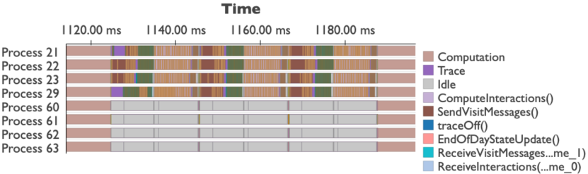
1bad_procs = idle_times["Process"].head(4)

2good_procs = idle_times["Process"].tail(4)

3

4loimos_64.filter("Process", "in", bad_procs + good_procs).plot_timeline()

Figure 15. Timeline view of a 64-process Loimos trace filtered to the most and least idling processes.

⬇

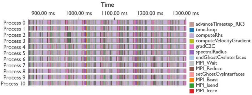
1tortuga_16 = pipit.Trace.from_otf2(’./tortuga_16’)

2matches = tortuga_16.detect_pattern(window_size, iterations, metric=’time.exc’)

3tortuga_16.plot_timeline()

Figure 16. Timeline view of a Tortuga trace after detecting patterns and filtering by time.

Similarly, in Figure 16, we use the output of the pattern_detection function to filter the timeline by a time range, which allows us to focus on one iteration of Tortuga.

8. Conclusion

In this paper, we present a new Python-based performance analysis tool called Pipit for analyzing parallel execution traces. Through Pipit’s design and implementation, we sought to solve the following challenges: (1) Support several file formats in which execution traces are collected to provide users with a unified interface that works with outputs of many different tracing tools. (2) Provide a programmatic API, which allows users to write simple code for trace analysis and provides several benefits such as flexibility of exploration, scalability, reproducibility, and automation/saving of workflows. And (3) Automate certain common performance analysis tasks for analyzing single and multiple executions. To the best of our knowledge, Pipit is unique in its capabilities in terms of supporting several file formats and providing a programmatic API to analyze traces. We believe that Pipit can revolutionize how HPC developers and performance engineers analyze the performance of their codes, and improve the efficiency of both parallel programs and HPC programmers.

References

- (1)
- per (2022) 2022. Perfetto - System profiling, app tracing and trace analysis. https://perfetto.dev/docs/. Accessed: 2023-04-01.
- Adhianto et al. (2010) Laksono Adhianto, Sinchan Banerjee, Mike Fagan, Mark Krentel, Gabriel Marin, John Mellor-Crummey, and Nathan R Tallent. 2010. HPCToolkit: Tools for performance analysis of optimized parallel programs. Concurrency and Computation: Practice and Experience 22, 6 (2010), 685–701.
- Bell et al. (2003) Robert Bell, Allen D Malony, and Sameer Shende. 2003. Paraprof: A portable, extensible, and scalable tool for parallel performance profile analysis. In European Conference on Parallel Processing. Springer, 17–26.
- Bhatele et al. (2019) Abhinav Bhatele, Stephanie Brink, and Todd Gamblin. 2019. Hatchet: Pruning the Overgrowth in Parallel Profiles. In Proceedings of the ACM/IEEE International Conference for High Performance Computing, Networking, Storage and Analysis (SC ’19). http://doi.acm.org/10.1145/3295500.3356219 LLNL-CONF-772402.
- Calotoiu et al. (2013) Alexandru Calotoiu, Torsten Hoefler, Marius Poke, and Felix Wolf. 2013. Using Automated Performance Modeling to Find Scalability Bugs in Complex Codes. In Proc. of the ACM/IEEE Conference on Supercomputing (SC13), Denver, CO, USA. ACM, 1–12. https://doi.org/10.1145/2503210.2503277
- Dobrev et al. (2012) Veselin A. Dobrev, Tzanio V. Kolev, and Robert N. Rieben. 2012. High-Order Curvilinear Finite Element Methods for Lagrangian Hydrodynamics. SIAM Journal on Scientific Computing 34, 5 (2012), B606–B641. https://doi.org/10.1137/120864672 arXiv:https://doi.org/10.1137/120864672
- Eschweiler et al. (2012) Dominic Eschweiler, Michael Wagner, Markus Geimer, Andreas Knüpfer, Wolfgang E Nagel, and Felix Wolf. 2012. Open trace format 2: The next generation of scalable trace formats and support libraries. In Applications, Tools and Techniques on the Road to Exascale Computing. IOS Press, 481–490.
- Geimer et al. (2010) Markus Geimer, Felix Wolf, Brian JN Wylie, Erika Ábrahám, Daniel Becker, and Bernd Mohr. 2010. The Scalasca performance toolset architecture. Concurrency and computation: Practice and experience 22, 6 (2010), 702–719.
- Henson and Yang (2002) Van Emden Henson and Ulrike Meier Yang. 2002. BoomerAMG: A parallel algebraic multigrid solver and preconditioner. Applied Numerical Mathematics 41, 1 (2002), 155–177. https://doi.org/10.1016/S0168-9274(01)00115-5 Developments and Trends in Iterative Methods for Large Systems of Equations - in memorium Rudiger Weiss.
- Kale and Bhatele (2013) Laxmikant V. Kale and Abhinav Bhatele (Eds.). 2013. Parallel Science and Engineering Applications: The Charm++ Approach. Taylor & Francis Group, CRC Press.
- Kale et al. (2006) Laxmikant V. Kale, Gengbin Zheng, Chee Wai Lee, and Sameer Kumar. 2006. Scaling Applications to Massively Parallel Machines Using Projections Performance Analysis Tool. In Future Generation Computer Systems Special Issue on: Large-Scale System Performance Modeling and Analysis, Vol. 22. 347–358.
- Knüpfer et al. (2008) Andreas Knüpfer, Holger Brunst, Jens Doleschal, Matthias Jurenz, Matthias Lieber, Holger Mickler, Matthias S. Müller, and Wolfgang E. Nagel. 2008. The Vampir Performance Analysis Tool-Set. In Tools for High Performance Computing, Michael Resch, Rainer Keller, Valentin Himmler, Bettina Krammer, and Alexander Schulz (Eds.). Springer Berlin Heidelberg, Berlin, Heidelberg, 139–155.
- Knüpfer et al. (2012) Andreas Knüpfer, Christian Rössel, Dieter an Mey, Scott Biersdorff, Kai Diethelm, Dominic Eschweiler, Markus Geimer, Michael Gerndt, Daniel Lorenz, Allen Malony, Wolfgang E. Nagel, Yury Oleynik, Peter Philippen, Pavel Saviankou, Dirk Schmidl, Sameer Shende, Ronny Tschüter, Michael Wagner, Bert Wesarg, and Felix Wolf. 2012. Score-P: A Joint Performance Measurement Run-Time Infrastructure for Periscope,Scalasca, TAU, and Vampir. In Tools for High Performance Computing 2011, Holger Brunst, Matthias S. Müller, Wolfgang E. Nagel, and Michael M. Resch (Eds.). Springer Berlin Heidelberg, Berlin, Heidelberg, 79–91.
- Kunen et al. (2015) AJ Kunen, TS Bailey, and PN Brown. 2015. KRIPKE-A massively parallel transport mini-app. Lawrence Livermore National Laboratory (LLNL), Livermore, CA, Tech. Rep (2015).
- Law (2019) Sean M. Law. 2019. STUMPY: A Powerful and Scalable Python Library for Time Series Data Mining. The Journal of Open Source Software 4, 39 (2019), 1504.
- McKinney (2017) Wes McKinney. 2017. Python for Data Analysis: Data Wrangling with Pandas, NumPy, and IPython. O’Reilly Media.
- NVIDIA ([n. d.]) NVIDIA. [n. d.]. NVIDIA Nsight Systems. https://developer.nvidia.com/nsight-systems.
- Saviankou et al. (2015) Pavel Saviankou, Michael Knobloch, Anke Visser, and Bernd Mohr. 2015. Cube v4: From performance report explorer to performance analysis tool. Procedia Computer Science 51 (2015), 1343–1352.
- Shende and Malony (2006) Sameer S Shende and Allen D Malony. 2006. The TAU parallel performance system. The International Journal of High Performance Computing Applications 20, 2 (2006), 287–311.
- Yeh et al. (2016) Chin-Chia Michael Yeh, Yan Zhu, Liudmila Ulanova, Nurjahan Begum, Yifei Ding, Hoang Anh Dau, Diego Furtado Silva, Abdullah Mueen, and Eamonn Keogh. 2016. Matrix Profile I: All Pairs Similarity Joins for Time Series: A Unifying View That Includes Motifs, Discords and Shapelets. In 2016 IEEE 16th International Conference on Data Mining (ICDM). 1317–1322. https://doi.org/10.1109/ICDM.2016.0179