Observations and chemical modeling of the isotopologues of formaldehyde and the cations of formyl and protonated formaldehyde in the hot molecular core G331.512-0.103

Abstract

In the interstellar cold gas, the chemistry of formaldehyde (H₂CO) can be essential to explain the formation of complex organic molecules. On this matter, the massive and energetic protostellar object G331 is still unexplored and, hence, we carried out a comprehensive study of the isotopologues of H₂CO and formyl cation (HCO⁺), and of protonated formaldehyde (H₂COH⁺) through the APEX observations in the spectral window $\sim$159–356 GHz. We employed observational and theoretical methods to derive the physical properties of the molecular gas combining LTE and non-LTE analyses. Formaldehyde was characterized via 35 lines of H₂CO, H${}_{2}^{13}$CO, HDCO and H₂C¹⁸O. The formyl cation was detected via 8 lines of HCO⁺, H¹³CO⁺, HC¹⁸O⁺ and HC¹⁷O⁺. Deuterium was clearly detected via HDCO, whereas DCO⁺ remained undetected. H₂COH⁺ was detected through 3 clean lines. According to the radiative analysis, formaldehyde appears to be embedded in a bulk gas with a wide range of temperatures ($T\sim$20–90 K), while HCO⁺ and H₂COH⁺ are primarily associated with a colder gas ($T\lesssim$ 30 K). The reaction H₂CO+HCO${}^{+}\rightarrow$ H₂COH⁺ + CO is crucial for the balance of the three species. We used Nautilus gas-grain code to predict the evolution of their molecular abundances relative to H₂ which values at time scales $\sim$10³ yr matched with the observations in G331: [H₂CO] = (0.2–2) $\times$10^-8, [HCO⁺] = (0.5–4) $\times$10^-9 and [H₂COH⁺] = (0.2–2) $\times$10^-10. Based on the molecular evolution of H₂CO, HCO⁺ and H₂COH⁺, we hypothesized about the young lifetime of G331, which is consistent with the active gas-grain chemistry of massive protostellar objects.

1 Introduction

Formaldehyde was one of the first organic molecules detected in the Interstellar Medium (ISM) (Snyder et al., 1969; Gardner & Whiteoak, 1974). This compound has been observed both in the gas and solid phase of the ISM (Meier et al., 1993; Schutte et al., 1996; Féraud et al., 2019). Formaldehyde also plays a key role in the interstellar synthesis of pre-biotic and complex organic molecules (Ferus et al., 2019; Layssac et al., 2020; Paiva et al., 2023).

In observational studies, Mangum et al. (1990) used maps and spectral lines of H₂CO to constrain the different components of the Orion Kleinmann–Low (KL) star forming region, which has been largely discussed in the context of cold, hot cores and molecular outflows (Wootten et al., 1984; Sutton et al., 1995; Zapata et al., 2011). Pegues et al. (2020) analyzed maps of H₂CO toward a sample of discs surveyed with ALMA. They highlighted the importance of H₂CO to understand the production mechanisms of O-bearing molecules in discs. In hot corinos and low-mass protostellar objects, H₂CO transitions have been useful to estimate its physical and chemical conditions (Maret et al., 2004; Sahu et al., 2018; Martín-Doménech et al., 2019). In the Horsehead photodissociation region, Guzmán et al. (2013) analyzed observations of H₂CO and CH₃OH to investigate their chemistry and dominant formation routes. In massive star forming regions, H₂CO transitions have been observed in hot molecular cores. In addition, an H₂CO maser at 6 cm has been proposed as an exclusive tracer of high-mass star formation (Pratap et al., 1994; Araya et al., 2015). In the IRAS 16562-3959 high-mass star-forming region, Taniguchi et al. (2020) observed H₂CO and investigate its formation pathways; they also analyzed the emission of (CH₃)₂CO and CH₃OCHO. The identification of both simple and complex organic molecules contributes to our understanding of the chemical network of reactions that interplay these species under interstellar conditions (e.g. Horn et al. 2004; Singh et al. 2022). In evolved stellar objects, Ford et al. (2004) observed H₂CO toward the carbon star IRC+10216 and discussed the H₂CO formation in the context of solar system comet comae. In sources outside the Milky Way, Tang et al. (2021) observed H₂CO to construct a map of the kinetic temperature of two massive star-forming regions in the Large Magellanic Cloud (LMC). Shimonishi et al. (2016) analyzed observations of H₂CO, among other chemical species, to diagnose and claim the first detection of a hot molecular core in the LMC.

The physical conditions of the formaldehyde isotopologues are also investigated here. In a study about deuterated molecules in Orion KL, Neill et al. (2013) estimated D/H ratios from formaldehyde and other molecules using data from Herschel/HIFI. As a rare isotopic species, Turner 1990 detected D₂CO via four transitions toward Orion-KL. Nonetheless, Neill et al. (2013) did not confirm such detection. In a sample of Galactic molecular sources, Yan et al. (2019) performed a study about the ¹²C/¹³C ratio using transitions from the H${}_{2}^{12}$CO and H${}_{2}^{13}$CO isotopologues. With respect to H₂C¹⁸O, a few works have reported its detection. Using ALMA observations, Persson et al. (2018) not only detected H₂C¹⁸O, but also H₂C¹⁷O, D${}_{2}^{13}$CO and HDC¹⁸O, toward IRAS 16293-2422 B.

In chemical association with H₂CO, we also present results about the molecular ions HCO⁺ and H₂COH⁺ (Fig. 1). HCO⁺ and its isotopologues have been observed in hot molecular cores and outflows (Sánchez-Monge et al., 2013; Shimonishi et al., 2016). In previous works, Merello et al. (2013) and Hervías-Caimapo et al. (2019) reported preliminary results about H¹³CO⁺ in G331.512-0.103, from now on G331. H₂COH⁺ is a rare molecular ion whose detection has been scarcely reported in the literature. It has been observed toward Sgr B2, Orion KL, W51 and the prestellar core L1689B (Ohishi et al., 1996; Bacmann et al., 2016).

H₂CO, HCO⁺ and H₂COH⁺ are chemical species that participate and compete in various chemical reactions, for instance:

$$\text{H_{2}CO+HCO^{+}\longrightarrow H_{2}COH^{+}+CO~{}~{}~{}.}$$ (1)

The kinetic constants were experimentally studied in an early work by Tanner et al. (1979). Bacmann et al. (2016) observed H₂COH⁺ in the prestellar source L1689B and discussed the reaction presented in Eq. 1 in the context of cold prestellar cores. The three species studied here, H₂CO, HCO⁺ and H₂COH⁺, also play a key role in the gas-grain chemistry to form complex organic molecules, such as glycolaldehyde and sugar related molecules (Halfen et al., 2006; Woods et al., 2012; Eckhardt et al., 2018; Layssac et al., 2020). Additionally, it is worth mentioning that H₂CO is closely associated with methanol (CH₃OH), a pivotal molecule for interstellar chemical complexity. Studies have demonstrated that successive hydrogenation reactions of carbon monoxide (CO) can lead to the formation of both H₂CO and CH₃OH (Watanabe et al., 2003; Tsuge et al., 2020).

The present work is based on observations of G331, a massive protostellar object embedded in the G331.5-0.1 giant molecular cloud. The central object drives a powerful outflow with a flow mass and momentum of $\sim 55~{}M_{\odot}$ and $\sim 2.4\times 10^{3}~{}M_{\odot}$ km s^-1, respectively (Bronfman et al., 2008). The source is located in the tangent region of the Norma spiral arm, at an heliocentric distance of $\sim$ 7.5 kpc. Regarding the ambient core of G331, ALMA observations evidence a lukewarm gas with $n_{\text{H}_{2}}\sim 5\times 10^{6}$ cm^-3 and $T\sim$ 70 K (Hervías-Caimapo et al., 2019). In association with those gas conditions, Canelo et al. (2021) and Santos et al. (2022) reported recent results about the physical and chemical conditions of the isocyanic acid (HNCO) and methyl acetylene (CH₃CCH). Here, we then contribute with new results about the lukewarm and cold gas conditions of G331, which are based on a broad spectral survey collected with the Atacama Pathfinder Experiment (APEX).

In massive protostellar objects, the chemical scenario about the formation of hydrocarbons, carbon chain and organic compounds is not well understood yet (Taniguchi et al., 2018; Kalvāns, 2021). In view of the importance to understand how gas-grain processes occur in massive protostellar objects, this work also presents a chemical model to understand the cold chemistry that connects two abundant species, as H₂CO and HCO⁺, with a low abundant ion as H₂COH⁺. In addition, this study allowed us to venture the age of the protostellar object G331. This article is organized as follows: Section 2 describes the observations carried out by APEX of the source G331 and the methodology used for this study. Section 3 presents the results of the spectral analysis and the estimated physical conditions of G331. In Section 4, the astrophysical and astrochemical implications of the present results are discussed. Final remarks and conclusions are summarized in Section 5. Additionally, an appendix section (A) has been included to provide supplementary information and data.

C(-[:-150]H)(-[:-30]H)=[:90]Oa) H-C O⊕b) C(-[:-150]H)(-[:-30]H)=[:90]O⊕-[:30]Hc)

Figure 1: Representation of the neutral molecule a) formaldehyde, and the molecular ions b) formyl cation and c) protonated formaldehyde.

2 Methodology

The APEX telescope (Güsten et al., 2006) was used to perform the observations, adopting the single point mode, toward the source coordinates RA:DEC = 16^h12^m10.1^s, $-$51^∘28^′38.1^′′. The APEX-1 and APEX-2 receivers, of the Swedish Heterodyne Facility Instrument (SHeFI) (Vassilev et al., 2008), were used to collect spectral setups in the frequency ranges 213–275 GHz and 267–378 GHz, respectively. The spectral resolution of the dataset was adjusted to be between $\sim$0.15 and 0.25 km s^-1 for a noise level of about 30 mK across the bands.

As part of the observational runs, the SEPIA B5 instrument (Belitsky et al., 2018) was used to collect setups between 159–211 GHz. SEPIA B5 is a dual-polarisation sideband-separated receiver. The lower and upper sideband (LSB and USB) are separated by 12 GHz. Each sideband is recorded by two XFFTS units of 2.5 GHz with a 1 GHz overlap. The Half Power Beam Width (HPBW) values, covered by the APEX receivers, are ranged from $\sim$ 17 to 39″, were estimated for each transition using 7.8″$\times$ 800/$\nu$[GHz] (Güsten et al., 2006; Quénard et al., 2017), where $\nu$ is the rest frequency of the spectra. With respect to the calibration uncertainty, Dumke & Mac-Auliffe (2010) discussed that lines of C¹⁸O (3–2) and ¹³CO (3–2) might reach uncertainties of $\sim$ 13 %, and lines of H₂CO and CH₃OH of up to $\sim$ 33 %. Considering that we observed different species through a multi-wavelength analysis, it was adopted an overall calibration uncertainty of 30 %.

The data reduction was carried out with the CLASS package of GILDAS. The spectra obtained from the APEX real-time calibration tool (Muders et al., 2006), in the CLASS data architecture, are in the corrected antenna temperature scale. For further clarity, we exhibit spectra in units of antenna temperature (K) with respect to the systemic velocity of G331 ($V_{\rm lsr}$ = -90 km s^-1). Additionally, all the spectra were smoothed to exhibit a common channel of 1 km s^-1. The Weeds extension of CLASS (Maret et al., 2011), along with the spectroscopic databases CDMS (Endres et al., 2016) and JPL (Pickett et al., 1998), were also used here. The CASSIS software was used to estimate the physical conditions from the spectral lines, which were utilized in the main beam temperature ($T_{mb}$) scale adopting the main-beam efficiencies $\eta_{mb}$ = 0.80, 0.75 and 0.73 for SEPIA180, APEX-1 and APEX-2, respectively. In order to evaluate beam dilution effects, a source size of 5″ was adopted for the G331 core, and of 15″ for an expanded region. Using the CASSIS tools, Local Thermodynamic Equilibrium analyses were performed using calculations and the population diagram method (Goldsmith & Langer, 1999; Mangum & Shirley, 2015; Roueff et al., 2021). Non-LTE calculations were carried out with the RADEX code (van der Tak et al., 2007) using rate coefficients from the LAMDA database.

2.1 Chemical models

The gas grain code Nautilus was used to compute abundances as a function of time from a network of gas and grain chemical reactions (Semenov et al., 2010; Reboussin et al., 2014; Ruaud et al., 2015, 2016). We focused on computing the abundances of H₂CO, HCO⁺ and H₂COH⁺ considering similar conditions to those obtained from the observations. Nautilus uses the KIDA database (Wakelam et al., 2015), which includes rate coefficients for a total of about 7509 reactions and 489 chemical species. For the solid state chemistry, it considers mantle and surface mechanisms as those investigated by Hasegawa & Herbst (1993) and Ghesquière et al. (2015). For the neutral and molecular ions analyzed in this work, there is a network of no more than 50 chemical reactions connecting them. The chemistry of HCO⁺ and H₂CO is significant and the detection of various of their isotopologues suggests gas-grain processes in cold environments. Previous studies unveiled a rich chemistry in lukewarm regions of G331 ($T_{g}\thickapprox$70 K) evidenced from various spectral lines of HNCO and CH₃CCH (Canelo et al., 2021; Santos et al., 2022). We expanded here the chemical models of G331 adopting a cold gas condition ($T_{g}\thickapprox$50 K), which might not only explain the abundances of H₂CO, HCO⁺ and H₂COH⁺ but also the eventual formation of more complex molecules.

3 Results

3.1 Line analysis

3.1.1 Formaldehyde and its isotopologues

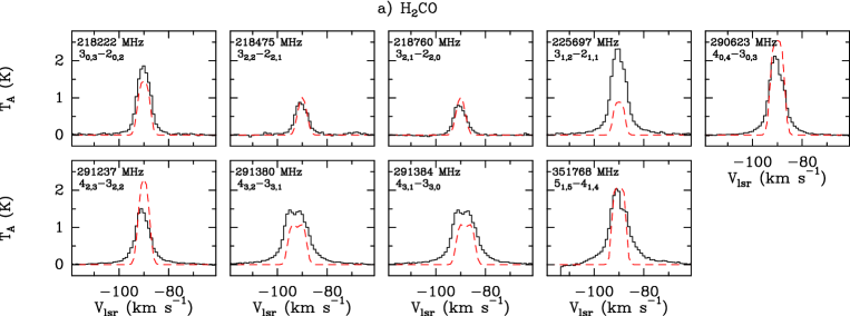
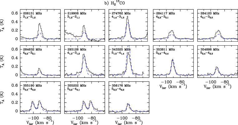
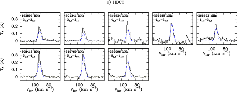
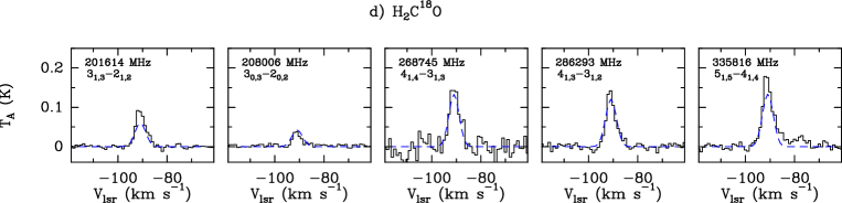
Figure 2: Observed (solid) and modelled (dashed) spectra, from the LTE (in blue) and non-LTE (in red) simulations (§ 3.2), of the formaldehyde isotopologues in G331: a) H₂CO, b) H${}_{2}^{13}$CO, c) HDCO and d) H₂C¹⁸O. For each spectrum, the $y$-axis represents the intensity in a scale of antenna temperature (K) while the $x$-axis represents the velocity relative to the local standard of rest (Systemic $V_{\rm lsr}=$ -90 km s^-1).

Table 1: Spectral line analysis of H${}_{2}^{12}$CO, H${}_{2}^{13}$CO, HDCO and H₂C¹⁸O.

Species and transitions	Frequency	Beamwidth	$E_{u}$	$g_{u}$	$A_{ul}$	Line area	$V_{\rm lsr}$	Linewidth	rms
	[MHz]	[″]	[K]		[10-5s-1]	[K km s-1]	[km s-1]	[km s-1]	[mK]
p-H2CO (3 0 3 – 2 0 2)	218222.192	28.56	20.96	7	28.2	12.99 $\pm$ 0.07	-90.07 $\pm$ 0.02	6.4 $\pm$ 0.04	47
p-H2CO (3 2 2 – 2 2 1)	218475.632	28.56	68.09	7	15.7	5.5 $\pm$ 0.3	-90.4 $\pm$ 0.1	5.9 $\pm$ 0.3	35
p-H2CO (3 2 1 – 2 2 0)	218760.066	28.52	68.11	7	15.8	5.04 $\pm$ 0.04	-90.33 $\pm$ 0.02	5.85 $\pm$ 0.05	36
o-H2CO (3 1 2 – 2 1 1)	225697.775	27.65	33.45	21	27.7	17.88 $\pm$ 0.06	-90.2 $\pm$ 0.01	7.25 $\pm$ 0.03	38
p-H2CO (4 0 4 – 3 0 3)	290623.405	21.47	34.9	9	69	16.1 $\pm$ 0.1	-90.39 $\pm$ 0.03	7.29 $\pm$ 0.08	42
p-H2CO (4 2 3 – 3 2 2)	291237.78	21.43	82.07	9	52.1	10.92 $\pm$ 0.03	-90.578 $\pm$ 0.009	7.13 $\pm$ 0.02	33
o-H2CO (4 3 2 – 3 3 1)	291380.488	21.41	140.94	27	30.4	9.653 $\pm$ 1E-3	-90.36 $\pm$ 0.02	6.73 $\pm$ 0.04	28
o-H2CO (4 3 1 – 3 3 0)	291384.264	21.41	140.94	27	30.4	12 $\pm$ 0.1	-90.38 $\pm$ 0.04	7.75 $\pm$ 0.09	29
o-H2CO (5 1 5 – 4 1 4)	351768.645	17.74	62.45	33	120	14.7 $\pm$ 0.2	-90.88 $\pm$ 0.04	7.1 $\pm$ 0.1	46
o-H${}_{2}^{13}$CO (3 1 3 – 2 1 2)	206131.626	30.27	31.62	21	21.1	1.68 $\pm$ 0.02	-90.91 $\pm$ 0.03	4.37 $\pm$ 0.08	18
o-H${}_{2}^{13}$CO (3 1 2 – 2 1 1)	219908.525	28.37	32.94	21	25.6	1.14 $\pm$ 0.04	-91.01 $\pm$ 0.06	3.6 $\pm$ 0.2	34
o-H${}_{2}^{13}$CO (4 1 4 – 3 1 3)	274762.112	22.71	44.8	27	54.7	2.49 $\pm$ 0.04	-90.94 $\pm$ 0.03	4.47 $\pm$ 0.08	32
o-H${}_{2}^{13}$CO (4 3 2 – 3 3 1)	284117.45	21.96	140.47	27	28.2	1.55 $\pm$ 0.05	-92.1 $\pm$ 0.1	7.3 $\pm$ 0.3	21
o-H${}_{2}^{13}$CO (4 3 1 – 3 3 0)	284120.62	21.96	140.47	27	28.2	1.1 $\pm$ 0.1	-90.5 $\pm$ 0.4	6.3 $\pm$ 0.7	18
p-H${}_{2}^{13}$CO (4 2 2 – 3 2 1)	284632.42	21.92	81.43	9	48.6	0.59 $\pm$ 0.02	-91.54 $\pm$ 0.05	3.4 $\pm$ 0.1	17
o-H${}_{2}^{13}$CO (4 1 3 – 3 1 2)	293126.515	21.29	47.01	27	66.4	2.25 $\pm$ 0.08	-91.2 $\pm$ 0.07	4.2 $\pm$ 0.2	42
o-H${}_{2}^{13}$CO (5 1 5 – 4 1 4)	343325.713	18.17	61.28	33	112	2.45 $\pm$ 0.09	-90.93 $\pm$ 0.07	4.3 $\pm$ 0.2	30
p-H${}_{2}^{13}$CO (5 0 5 – 4 0 4)	353811.872	17.64	51.02	11	127	1.54 $\pm$ 0.04	-91.22 $\pm$ 0.05	3.8 $\pm$ 0.1	33
p-H${}_{2}^{13}$CO (5 2 4 – 4 2 3)	354898.595	17.58	98.41	11	108	0.83 $\pm$ 0.05	-91.3 $\pm$ 0.1	4.0 $\pm$ 0.3	34
o-H${}_{2}^{13}$CO (5 3 3 – 4 3 2)	355190.9	17.57	157.52	33	82.5	1.39 $\pm$ 0.04	-90.81 $\pm$ 0.08	5.9 $\pm$ 0.2	29
o-H${}_{2}^{13}$CO (5 3 2 – 4 3 1)	355202.601	17.57	157.52	33	82.5	1.21 $\pm$ 0.03	-90.79 $\pm$ 0.07	5.1 $\pm$ 0.2	32
p-H${}_{2}^{13}$CO (5 2 3 – 4 2 2)	356176.243	17.52	98.52	11	109	1.02 $\pm$ 0.03	-91.04 $\pm$ 0.08	5.2 $\pm$ 0.2	32
HDCO (3 0 3 – 2 0 2)	192893.27	32.35	18.53	7	19.4	1.03 $\pm$ 0.02	-90.73 $\pm$ 0.06	5.2 $\pm$ 0.1	21
HDCO (3 1 2 – 2 1 1)	201341.35	30.99	27.29	7	19.6	0.956 $\pm$ 0.008	-91.02 $\pm$ 0.02	5.25 $\pm$ 0.05	18
HDCO (4 1 4 – 3 1 3)	246924.6	25.27	37.6	9	39.6	1.06 $\pm$ 0.04	-90.73 $\pm$ 0.09	4.3 $\pm$ 0.2	47
HDCO (4 0 4 – 3 0 3)	256585.43	24.32	30.85	9	47.4	1.25 $\pm$ 0.05	-91.11 $\pm$ 0.08	4.6 $\pm$ 0.2	50
HDCO (4 1 3 – 3 1 2)	268292.02	23.26	40.17	9	50.8	0.85 $\pm$ 0.03	-91.06 $\pm$ 0.09	4.1 $\pm$ 0.2	37
HDCO (5 1 5 – 4 1 4)	308418.2	20.23	52.4	11	80.8	1.54 $\pm$ 0.02	-91.14 $\pm$ 0.02	4.72 $\pm$ 0.07	20
HDCO (5 0 5 – 4 0 4)	319769.68	19.51	46.19	11	93.7	1.41 $\pm$ 0.03	-91.31 $\pm$ 0.05	4.5 $\pm$ 0.1	37
HDCO (5 1 4 – 4 1 3)	335096.739	18.62	56.25	11	104	1.43 $\pm$ 0.02	-91.04 $\pm$ 0.04	4.76 $\pm$ 0.09	28
o-H2C18O (3 1 3 – 2 1 2)	201614.256	30.95	31.22	21	19.7	0.473 $\pm$ 0.009	-90.83 $\pm$ 0.05	4.8 $\pm$ 0.1	18
p-H2C18O (3 0 3 – 2 0 2)	208006.441	29.99	19.97	7	24.4	0.134 $\pm$ 0.007	-91.17 $\pm$ 0.09	3.4 $\pm$ 0.2	17
o-H2C18O (4 1 4 – 3 1 3)	268745.789	23.22	44.12	27	51.1	0.76 $\pm$ 0.04	-90.7 $\pm$ 0.1	4.9 $\pm$ 0.3	48
o-H2C18O (4 1 3 – 3 1 2)	286293.96	21.79	46.23	27	61.8	0.64 $\pm$ 0.02	-91.01 $\pm$ 0.06	4.3 $\pm$ 0.2	23
o-H2C18O (5 1 5 – 4 1 4)	335816.025	18.58	60.24	33	105	0.85 $\pm$ 0.02	-90.99 $\pm$ 0.06	4.8 $\pm$ 0.1	24

.

The isotopologues H${}_{2}^{12}$CO, H${}_{2}^{13}$CO, HDCO and H₂C¹⁸O were identified in the frequency interval $\sim$ 190–357 GHz through 35 transition lines whose assignments, specifying the ortho or para character of the states for the symmetric isotopologues (e.g. Clouthier & Ramsay 1983; Chapovsky 2001), spectroscopic data and Gaussian fit parameters are given in Table 1. The spectral analysis was primarily performed on lines with significantly stronger signals than the limit of detection (3$\sigma$ level), which are exhibited in the different panels of Fig. 2. In agreement with the expected isotopic abundances, the most and least abundant isotopologues, H${}_{2}^{12}$CO and H₂C¹⁸O, respectively, exhibited the strongest and weakest line intensities, respectively. Despite H₂C¹⁸O is a rare isotopologue (e.g., Müller & Lewen 2017), we could detect it via 5 spectral lines.

The main isotopologue (o, p)-H₂CO was detected via 9 lines although the lines at $\sim$ 291380.48 and 291384.26 MHz, corresponding to the transitions 4_3,2-3_3,1 and 4_3,1-3_3,0, respectively, can be considered partially resolved (see Fig 2(a)). Various of the H₂CO transitions detected in this work were also reported in sources as OMC-1, Orion-KL and in high-mass star-forming regions (e.g. Loren 1984; Wootten et al. 1984; Mangum et al. 1990; Taniguchi et al. 2020).

13 spectral lines of (o, p)-H${}_{2}^{13}$CO were identified although two of them at the rest frequencies $\sim$ 284117.45 and 284120.62 MHz were deemed as partially resolved (see Fig 2(b)). As it is expected, the intensities of the H${}_{2}^{13}$CO lines are lower than those of H₂CO. By comparing the integrated areas of neighbor lines, e.g., o-H${}_{2}^{13}$CO at $\sim$ 219908.52 MHz and o-H₂CO at $\sim$ 225697.77 MHz, the H₂CO/H${}_{2}^{13}$CO ratio is about 16. In previous works, Jewell et al. (1989) and Helmich & van Dishoeck (1997) observed various of the H${}_{2}^{13}$CO transitions in G331.

The HDCO isotopologue was detected via 8 spectral lines (see Fig. 2(c)). It can be noted that the HDCO line profiles exhibit a partial asymmetry with a blue-shifted emission wing. In an investigation on HNCO in G331, Canelo et al. (2021) not only observed similar spectral asymmetries but also found them to be more pronounced in some specific $K$-ladder transitions of HNCO. These findings were discussed in the context of molecular outflows (e.g. Canelo et al. 2021 and references therein). In this work, we expect that the HDCO emission may be linked to an expanded gas region influenced by the molecular outflow. However, to better understand the emission of spectral tracers potentially associated with the molecular outflow, it is crucial to conduct further investigations, including the development of models that consider the core and outflow of G331.

In addition, 5 spectral lines of (o, p)-H₂C¹⁸O isotopologue were clearly identified and shown in Fig. 2(d). From this study toward G331, we confirm the observation of the transitions of the rare isotopologue H₂C¹⁸O previously reported toward other sources (e.g., Mangum et al. 1990; Sutton et al. 1995).

The successful detection of HDCO prompted further investigation into the presence of the doubly deuterated formaldehyde (D₂CO), which has been scarcely observed in objects of the ISM (e.g., Turner 1990; Ceccarelli et al. 1998). As a result, we report the tentative detection of p-D₂CO 3_1,3–2_1,2 at the rest frequency $\sim$ 166102.74 MHz previously detected in prestellar cores (Bacmann et al., 2003). Fig. 3(a) shows this spectral line whose emission is above the limit of detection although shifted from the source systemic velocity ($V_{\rm lsr}=-90$ km s^-1). This makes us think that a possible candidate for this line might also be OC³⁴S (14–13) at 166105.75 MHz. A second tentative identification is displayed in Fig. 3b, the o-D₂CO 5_0,5–4_0,4 transition was also tentatively identified but a dominant line, likely blended with SO₂ v=0 at $\sim$ 287485.44 MHz, avoided a clear identification.

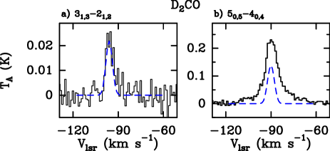
Figure 3: Tentative identification of D₂CO: a) p-D₂CO 3_1,3–2_1,2 at the frequency $\sim$ 166102.74 MHz and appearing at $V_{\rm lsr}\thickapprox-96$ km s^-1; b) o-D₂CO 5_0,5–4_0,4 at the frequency $\sim$ 287485.65 MHz but likely dominated by emission of SO₂ at 287485.44 MHz. Under the upper limit condition $N$(D₂CO)$<N$(HDCO), and FWHM=5 km s^-1, the dashed lines indicate hypothetical LTE models of D₂CO.

3.1.2 The formyl cation and its isotopologues

The isotopologues of formyl cation (HCO⁺, H¹³CO⁺, DCO⁺, HC¹⁸O⁺ and HC¹⁷O⁺) were also sought in G331. Eight lines from these isotopologues were identified, except the deuterated one DCO⁺, of which their spectroscopic and fitted parameters are given in Table 2. The two rotational lines of the main isotopologue HCO⁺ and their fits are shown in Fig. 4. The HCO⁺ spectra exhibited broad spectral wings, from $-$150 km s^-1 to $-$30 km s^-1, and they were better described by Lorentzian than Gaussian functions. The Lorentzian profile suggests that the HCO⁺ emission is likely affected by the molecular outflow (Hervías-Caimapo et al., 2019).

Figure 4: Spectral lines (solid lines) and Lorentzian fits (dotted lines) of the transitions 2–1 and 3–2 of HCO⁺ identified at the rest frequencies $\sim$ 178375.05 MHz and 267557.62 MHz, respectively.

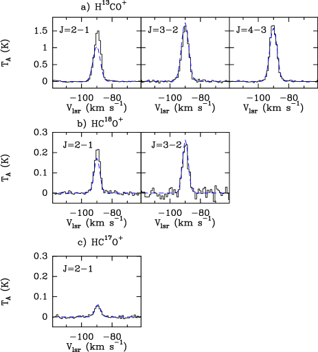
Figure 5: Legend similar to that of Fig. 2 but for the isotopologues of the formyl cation, with their LTE models: a) H¹³CO⁺, b) HC¹⁸O⁺ and c) HC¹⁷O⁺.

The spectral lines of H¹³CO⁺, HC¹⁸O⁺ and HC¹⁷O⁺ did not exhibit Lorentzian profiles with broad wings. Thus, Gaussian functions, instead of Lorentzian ones, were used to fit the spectra. The spectra of these isotopologues are exhibited in the different panels of Fig. 5. For all the identified HCO⁺ isotopologues, the $J$=2–1 transition was observed. Considering the velocity integrated temperatures for the line profiles of this transition, the ratios HCO⁺:H¹³CO⁺:HC¹⁸O⁺:HC¹⁷O${}^{+}\thickapprox$ 64:21:3:1 were obtained. Nevertheless, the results based on LTE and non-LTE methods will be given in the next section.

It is worth highlighting that the deuterated formyl cation DCO⁺ was not detected in spite of the isotopologue HDCO was identified through several lines. In contrast, the ¹⁷O isotopologue of formyl cation was detected but not the isotopologue of formaldehyde H₂C¹⁷O. Those aspects demand follow-up studies due to their implications on the understanding of the isotopic fraction and the evolution of protostellar objects.

3.1.3 Protonated formaldehyde

The search for H₂COH⁺ was performed across the frequency range $\sim$ 159–356 GHz. As a result, the identified lines of H₂COH⁺ are exhibited in Fig. 6 and were adjusted by means of Gaussian functions. The spectroscopic and fit parameters are listed in Table 2. In Fig. 6, the first three spectra were identified without blended emission at the rest frequencies $\sim$ 190079.13, 207964.75 and 252870.34 MHz; on the fourth display, a tentative identification was made at $\sim$348102.33 MHz, the detection is unclear due to a spectral signature which dominates the whole spectrum, it is likely associated with ³⁴SO₂ at $\sim$ 348117 MHz (e.g. Jewell et al. 1989).

In this work, the detection of H₂COH⁺ is reported for the first time in a hot molecular core as G331. This cation was identified by Ohishi et al. (1996), across the frequency range $\sim$ 31–174 GHz, toward massive star-forming regions but not in cold and dark clouds. Bacmann et al. (2016) detected H₂COH⁺, across the frequency range $\sim$ 102–168 GHz, in a cold ($\sim$ 10 K) source, the prestellar core L1689B. By means of a different technique of observation, Meier et al. (1993) detected H₂COH⁺ in the coma of comet P/Halley through a Neutral Mass Spectrometer on the Giotto spacecraft.

Table 2: Spectral line analysis of the molecular ions HCO⁺, H¹³CO⁺, HC¹⁸O⁺, HC¹⁷O⁺ and H₂COH⁺.

Species and transitions	Frequency	Beamwidth	$E_{u}$	$A_{ul}$	Line area	$V_{\rm lsr}$	Linewidth	rms
	[MHz]	[″]	[K]	[10-5s-1]	[K km s-1]	[km s-1]	[km s-1]	[mK]
HCO+ (2 – 1)a	178375.056	34.98	12.84	40.2	20 $\pm$ 2	-91.56 $\pm$ 0.02	6.97 $\pm$ 0.07	120
HCO+ (3 – 2)a	267557.626	23.32	25.68	145	31 $\pm$ 3	-91.21 $\pm$ 0.03	9.2 $\pm$ 0.1	133
H13CO+ (2 – 1)	173506.700	35.96	12.49	37	6.41 $\pm$ 0.02	-89.631 $\pm$ 0.006	4.93 $\pm$ 0.01	13
H13CO+ (3 – 2)	260255.339	23.97	24.98	134	7.05 $\pm$ 0.05	-89.94 $\pm$ 0.02	5.14 $\pm$ 0.04	53
H13CO+ (4 – 3)	346998.344	17.98	41.63	329	6.25 $\pm$ 0.02	-90.205 $\pm$ 0.007	5.19 $\pm$ 0.02	22
HC18O+ (2 – 1)	170322.626	36.63	12.26	35	1.05 $\pm$ 0.01	-89.69 $\pm$ 0.03	4.37 $\pm$ 0.07	11
HC18O+ (3 – 2)	255479.389	24.42	24.52	127	1.14 $\pm$ 0.04	-89.86 $\pm$ 0.08	4.5 $\pm$ 0.2	44
HC17O+ (2 – 1)	174113.169	35.83	12.53	37.4	0.31 $\pm$ 0.01	-89.5 $\pm$ 0.1	5.1 $\pm$ 0.3	11
H2COH+ (3 0 3 – 2 0 2)	190079.131	32.82	18.26	6.59	0.16 $\pm$ 0.01	-89.9 $\pm$ 0.2	4.5 $\pm$ 0.5	12
H2COH+ (5 1 4 – 5 0 5)	207964.754	30.00	55.51	14.7	0.12 $\pm$ 0.01	-91.6 $\pm$ 0.2	5.6 $\pm$ 0.8	17
H2COH+ (4 0 4 – 3 0 3)	252870.339	24.67	30.39	16.1	0.23 $\pm$ 0.05	-90.7 $\pm$ 0.3	3.2 $\pm$ 0.9	44
H2COH+ (10 1 9 – 10 0 10)b	348102.330	17.92	181.67	48.2	0.4 $\pm$ 0.1	-91.6 $\pm$ 0.4	7 $\pm$ 2	30

a)The line fit parameters of the HCO⁺ lines were obtained using Lorentzian functions. b)Line likely blended with ³⁴SO₂.

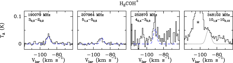
Figure 6: Legend similar to Fig. 2 but for the spectral lines of H₂COH⁺ with their LTE models (dashed lines). In the fourth panel, the Gaussian fit depicts an H₂COH⁺ transition tentatively identified at $\sim$ 348102.330 MHz. The asterisk indicates a line likely blended with ³⁴SO₂ at $\sim$ 348117 MHz.

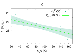
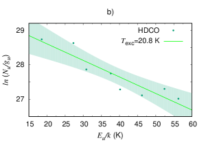
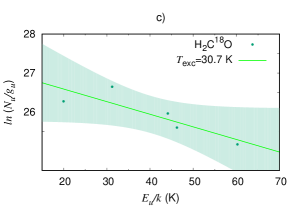
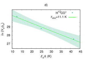
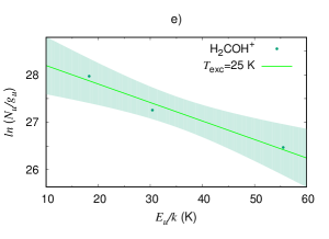
Figure 7: Population diagrams of the formaldehyde isotopologues a) H${}_{2}^{13}$CO, b) HDCO and c) H₂C¹⁸O; and of the molecular ions d) H¹³CO⁺ and e) H₂COH⁺. The solid-line and shaded areas represent the linear regression fits and their (95%) confidence bands for each species.

3.2 Physical conditions

The temperature and the column densities of the molecular species were estimated using LTE and Non-LTE conditions. LTE methods were applied to analyze the physical conditions of all the detected isotopologues of formaldehyde, the formyl cation and the protonated formaldehyde (H₂COH⁺). Non-LTE hypotheses were considered to infer the physical conditions of the ¹²C isotopologues, H₂CO and HCO⁺. All the analyses were performed under the general assumption of a source size of 5″. In the particular case of HCO⁺, a second solution adopting 15″was tested too.

When the LTE approximation is assumed, the population diagram method was used to estimate the excitation conditions of the molecular species, i.e., the total column densities ($N$) and excitation temperatures ($T_{\rm exc}$) by means of

$$\ln\frac{N_{u}}{g_{u}}=\ln\frac{N}{Q}-\frac{E_{u}}{kT_{\rm exc}},$$ (2)

where $N_{u}$, $g_{u}$, $E_{u}$ and $Q$ are the column density, the degeneracy of the upper state, the energy of the upper level involved in the transition and the partition function, respectively. In Table 1, the upper state degeneracy $g_{u}=(2J_{u}+1)g_{ns}^{(u)}$ was given for each detected transition, where $J_{u}$ and $g_{ns}^{(u)}$ are the rotational angular momentum and the nuclear spin statistical weight of the upper state (Bunker & Jensen, 1989). The optical depth ($\tau$) has been inferred using the population diagram method. For a given transition, this can be estimated using the following expression

$$\tau=\frac{c^{3}A_{ul}N_{u}}{8\pi\nu^{3}\Delta v\sqrt{\pi}/2\sqrt{\ln 2}}[\exp(h\nu/kT_{\rm exc})-1],$$ (3)

where $\Delta v$ and $A_{ul}$ represent the spectral linewidth (km s^-1) and the Einstein coefficients (s^-1), respectively (Goldsmith & Langer, 1999; Mangum & Shirley, 2015; Vastel et al., 2015).

3.2.1 Formaldehyde isotopologues: LTE analyses

The population diagrams of the ¹³C, D and ¹⁸O isotopologues of formaldehyde have been obtained with updated values of the partition function (see A) and Eq. (2) can be corrected taking into account the optical depth ($\tau$) applied when the gas emission tends to be optically thick, and beam dilution factors, which allows us to constrain the size of the emitting region with respect to the antenna beam (Goldsmith & Langer, 1999). The population diagrams of H${}_{2}^{13}$CO, HDCO and H₂C¹⁸O are exhibited in Fig. 7 (panels a, b and c, respectively) and were obtained after applying a beam dilution correction for an emitting source assumed to be 5″ and observed with an antenna beam ranged from $\sim$ 17 to 39″.

H${}_{2}^{13}$CO: Its population diagram was plotted using the 13 detected lines corresponding to transitions in the $E_{u}\thickapprox 31-158$ K range (Fig. 7a). The linear fit provided the result $T_{\rm exc}=82.9\pm 21.8$ K and $N=(8.0\pm 2.0)\times 10^{14}$ cm^-2 ($\chi^{2}_{\rm red}$=1.53). From this result, synthetic spectra were computed and compared with the observed lines in Fig. 2. The values of the optical depth were estimated $\tau\lesssim 1$ for all the spectra, except for the partially blended lines at $\sim$ 284117.45 and 284120.62 MHz, in agreement with the LTE formalism.

In comparison with previous works, Schöier et al. (2002) carried out radiative analyses of H${}_{2}^{13}$CO based on transitions in the $E_{u}\thickapprox 21-99$ K range toward the low-mass protostellar object IRAS 16293-2422. They reported an excitation temperature around 90 K.

HDCO: Based on its 8 spectral lines, detected in the range $E_{u}\thickapprox$ 18–56 K, the population diagram is displayed in Fig. 7(b). From the linear fit, it was obtained $T_{\rm exc}$ = 20.8 $\pm$ 3.5 K and $N$ = (2.5 $\pm$ 0.8) $\times$ 10¹⁴ cm^-2 ($\chi^{2}_{\rm red}$=0.84). The observed spectral lines and the simulated ones obtained from this result are exhibited in Fig. 2, the values of the optical depth were estimated $\tau\lesssim 1$.

Neill et al. (2013) performed a study about deuterated molecules in Orion KL. They discussed for H${}_{2}^{13}$CO and HDCO different LTE scenarios with temperatures of $\sim$ 40, 63, and 67 K as well as particular aspects about the deprotonation of H₂COH⁺ and HDCOH⁺. Bianchi et al. (2017) analyzed several deuterated species toward the Class I protostar SVS13-A. From the population diagrams of H${}_{2}^{13}$CO, HDCO and D₂CO, with source sizes of $\sim$ 10″, they derived temperatures of $\sim$ 23, 15, and 28 K, respectively.

D₂CO: LTE calculations were carried out to estimate an upper limit on the D₂CO emission. Taking into account the excitation conditions of HDCO, the D₂CO column density was computed assuming that $N$(D₂CO) $<N$(HDCO)$\thickapprox$2.5$\times$10¹⁴ cm^-2 and $T_{\rm exc}\thickapprox$ 21 K. The best solution gave $N$(D₂CO) $\thickapprox$ 1.3 $\times$ 10¹⁴ cm^-2 ($\chi^{2}_{\rm red}$=0.8) providing a column density ratio of D₂CO/HDCO $\thickapprox$ 0.5.

D₂CO has been observed in only few sources. In Orion KL, Neill et al. (2013) established an upper limit on the D₂CO abundance of [D₂CO]/[HDCO]$\leq$0.1. Turner (1990) detected three transitions of D₂CO in Orion KL reporting [D₂CO]/[HDCO]=0.02. In IRAS 16293-2422, a source with several studies on molecular deuteration, Ceccarelli et al. (1998) found [D₂CO]/[HDCO]$\leq$0.5.

H₂C¹⁸O: The population diagram of this isotopologue was obtained from 5 detected transition lines which covered the $E_{u}\thickapprox$ 19–60 K range. The linear fit provided $T_{\rm exc}$ = 30.7 $\pm$ 10.3 K and $N$ = (6.8 $\pm$ 3.2) $\times$ 10¹³ cm^-2 ($\chi^{2}_{\rm red}$=1.23). From this solution, synthetic spectra were simulated and compared with the observed lines (Fig. 2). The spectral lines of H₂C¹⁸O are optically thin, as expected according to its low abundance. It is worth mentioning that the population diagrams of HDCO and H₂C¹⁸O have similar $E_{u}$ ranges, between $\sim~{}18-60$ K, different from those of H${}_{2}^{13}$CO within $E_{u}\sim$ 30–160 K. The excitation temperatures of HDCO and H₂C¹⁸O ($T_{\rm exc}\lesssim$ 30 K) are lower than the obtained one for H${}_{2}^{13}$CO ($T_{\rm exc}\thickapprox$ 83 K). On the one hand, such difference might come from the fact that more lines of H${}_{2}^{13}$CO were observed than HDCO and H₂C¹⁸O, providing a more extended population diagram. On the other hand, there might be a scenario in which the formaldehyde isotopologues trace different excitation conditions although, to assume this hypothesis would require further studies including, e.g., gas-grain calculations and chemical models.

3.2.2 H₂CO: Non-LTE calculations

The physical conditions of H₂CO were calculated using the non-LTE code RADEX, which provides an alternative approach to the population diagram based on the assumption of optically thin emission lines. Within this approach, the optical depth effects are treated with an escape probability method assuming an isothermal and homogeneous medium without large-scale velocity fields (van der Tak et al., 2007). The non-LTE calculations were performed using available excitation rates between o- and p-H₂CO and o- and p-H₂. Wiesenfeld & Faure (2013) reported calculations for the first 81 rotational levels of formaldehyde considering temperatures between $\sim$ 10 and 300 K. In an earlier work, Troscompt et al. (2009) also discussed the rotational excitation of H₂CO by H₂.

From the five lines of p-H₂CO, the best solution ($\chi^{2}_{\rm red}$=4.5) provided $T_{\rm kin}=87.4\pm 0.6$ K and $N=(6.2\pm 0.3)\times 10^{15}$ cm^-2. From the four lines of o-H₂CO, it was obtained $T_{\rm kin}=95.1\pm 0.3$ K and $N=(9\pm 3)\times 10^{15}$ cm^-2 ($\chi^{2}_{\rm red}$=3.5). These results provide a ortho-to-para ratio of H₂CO of $\sim$ 1.4. The H₂ density was also estimated from the calculations $n({\rm H_{2}})\simeq 4\times 10^{7}$ cm^-3 adopting a source size of 5″. The density of molecular hydrogen was computed using conventional ortho-to-para ratios, whose value can fluctuate between $\sim$0.1 and 3, contingent on the chemistry, the physical properties and the evolutionary stage of sources. In prestellar cores, such a range was discussed from 3 to values even smaller than 0.001 (e.g. Osterbrock 1962; Lacy et al. 1994; Pagani et al. 2013).

Synthetic lines were generated from the non-LTE approximations and compared with the observations in Fig. 2(a). Concerning the optical depth of the p-H₂CO transitions, the highest and lowest values were $\sim$ 4.5 and 0.9 for the lines at $\sim$ 290623.40 MHz and 218760.06 MHz, respectively. Similarly, for the o-H₂CO transitions, the highest and lowest optical depths were $\sim$ 5.2 and $\sim$ 0.7 for the transitions at $\sim$ 351768.64 MHz and 291380 MHz, respectively.

A comparison of our results with other works is useful to show they are in accordance. Schöier et al. (2002) analysed the physical conditions of H₂CO in IRAS 16293-2422. They estimated temperatures around 90 K and ortho-to-para ratios of H₂CO around 0.9. Guzmán et al. (2013) used non-LTE models of o- and p-H₂CO based on observations with the IRAM-30m toward the Horsehead photo-dissociation region (PDR) to estimate ortho-to-para ratios around 3 at the dense core and 2 in the PDR. In a pioneering work, Mangum et al. (1990) stressed the importance of H₂CO as a key tracer to estimate density, temperature and molecular abundances. They performed LTE and non-LTE calculations obtaining $n$(H₂)=(0.5–1)$\times$10⁷ cm^-3 and $T_{\rm kin}\thickapprox$100 K in Orion KL. In this work we detected various lines of formaldehyde that were identified in Orion KL by Mangum et al. (1990).

3.2.3 Formyl cation isotopologues: LTE analyses

The population diagram obtained for H¹³CO⁺ using the three detected lines is exhibited in Fig. 7(d). Assuming that the emitting region is 5″, the excitation temperature and the column density were estimated, $T_{\rm exc}$ = 11 $\pm$ 1 K and $N$ = (2.1 $\pm$ 0.7) $\times$ 10¹⁴ cm^-2 ($\chi^{2}_{\rm red}$=1.30), respectively. In the case of HC¹⁸O⁺ and HC¹⁷O⁺, no population diagram could be displayed because of the lack of enough detected lines. Nevertheless, LTE calculations were performed to estimate their column densities. Similar methodologies were discussed in Schöier et al. (2002), who performed LTE and non-LTE calculations for HCO⁺ and its isotopologues in IRAS 16293-2422.

In this work the LTE calculations of HC¹⁸O⁺ and HC¹⁷O⁺ were performed fixing the excitation temperature to the value obtained for H¹³CO⁺ and considering the column densities as free parameters with the following condition $N$(HC¹⁷O⁺) $<N$(HC¹⁸O⁺) $<N$(H¹³CO⁺). The estimates of the column densities were $N$(HC¹⁸O⁺) $\thickapprox$ 1.8 $\times$10¹³ cm^-2 ($\chi^{2}_{\rm red}$=1.5) and $N$(HC¹⁷O⁺) $\thickapprox$ 1.4 $\times$10¹³ cm^-2 ($\chi^{2}_{\rm red}$=0.3). Synthetic spectra were included in the panels of Fig. 5.

The low temperature estimated from the H¹³CO⁺ lines suggests that its emission is likely associated with a cold and expanded region. In addition, we also obtained results assuming an extended source size of 15″. Thus, the H¹³CO⁺ population diagram gave the values $T_{\rm exc}$ = 12 $\pm$ 2 K and $N$ = (2.6 $\pm$ 0.8) $\times$ 10¹³ cm^-2, and for the ¹⁸O and ¹⁷O isotopologues $N$(HC¹⁸O⁺) $\thickapprox$ 4.2 $\times$10¹² cm^-2 and $N$(HC¹⁷O⁺) $\thickapprox$ 1.5 $\times$10¹² cm^-2.

3.2.4 HCO⁺: Non-LTE calculations

The main isotopologue HCO⁺ was observed through two intense and optically thick lines (Fig. 4), they were analyzed via non-LTE calculations using collisional excitation rates. The two transitions 2–1 and 3–2 were computed using RADEX and the rate coefficients available in the LAMDA database (Flower, 1999) assuming $n$(H₂)=(0.1–5)$\times$10⁷ cm^-3, $T<$ 30 K and 5″. The column density resulted in $N$(HCO⁺) $\thickapprox$ 3 $\times$ 10¹⁵ cm^-2 ($\chi^{2}_{\rm red}$=6.5). In the literature, line analysis of HCO⁺ has been reported with high reduced values of $\chi^{2}$ (Schöier et al., 2002). The result reported in this work should be taken as a rough approximation.

3.2.5 Protonated formaldehyde: LTE analysis

The 3 unblended lines of H₂COH⁺ allowed us to obtain the population diagram shown in Fig. 7(e) and the estimates $T_{\rm exc}$ = 25 $\pm$ 4 K and $N$ = (1.4 $\pm$ 0.3) $\times$ 10¹⁴ cm^-2 ($\chi^{2}_{\rm red}$=0.41) assuming a source size of 5″. Fig. 6 exhibits a comparison between the simulated and the observed lines with the exception of the spectrum affected by contaminant emission.

In comparison with other works, Ohishi et al. (1996) reported $T_{\rm exc}=60-110$ K and $N$(H₂COH⁺)$\thickapprox$10¹²–10¹⁴ cm^-2 in surveys toward Sgr B2, Orion KL and W51. In W51, since they could not detect a sufficient number of lines of H₂COH⁺, they used HCO⁺ to infer the physical conditions of H₂COH⁺ taking different excitation temperatures. In the ultra cold ($T\sim$10 K) source L1689B, Bacmann et al. (2016) estimated column densities between 3 $\times$ 10¹¹ cm^-2 and 1 $\times$ 10¹² cm^-2. They discussed that the H₂COH⁺ formation can occur via:

$$\text{H_{2}CO\ +\ x^{+}\longrightarrow H_{2}COH^{+}+H_{2}},$$ (4)

where x⁺ represents a proton donor such as H${}_{3}^{+}$. Furthermore, in the context of Eq. 1, the specific proton donor is HCO⁺ obtaining CO as a by-product instead of H₂. They predicted the abundance ratios [H₂COH${}^{+}]\thickapprox$ 0.007[H₂CO], when H${}_{3}^{+}$ is the proton donor, and [H₂COH${}^{+}]\thickapprox$ 0.003 [H₂CO], when it is HCO⁺.

In summary, we present in Table 3 the results obtained from the LTE and non-LTE analyses of the isotopologues of formaldehyde and the formyl. The results suggest that these species might trace different gas components. From the estimated column densities of the formaldehyde isotopologues, it was obtained the abundance ratios H₂CO:H${}_{2}^{13}$CO:HDCO:H₂C¹⁸O$\thickapprox$223:12:4:1. In addition, Table 3 also presents the results obtained from the population diagram of H₂COH⁺.

Table 3: Summary of the LTE and non-LTE analyses of the isotopologues of formaldehyde and the formyl cation, and the protonated formaldehyde. The temperatures and column densities come from the results obtained at a source size of 5″.

Species	# Analysed	Method	$N$ [cm-2]	$T$ [K]
	lines		$\thickapprox$	$\thickapprox$
H2CO	9	non-LTEa	1.52 $\times$ 1016	91
H${}_{2}^{13}$CO	13	LTEb	8.0 $\times$ 1014	83
HDCO	8	LTEb	2.5 $\times$ 1014	21
H2C18O	5	LTEb	6.8 $\times$ 1013	31
D2CO	2	LTEc	$<$1.3 $\times$ 1014	21
HCO+	2	non-LTE	3$\times$1015	$<$30
H13CO+	3	LTEb	2.1$\times$1014	11
HC18O+	2	LTEd	1.8$\times$1013	11
HC17O+	1	LTEd	1.4$\times$1013	11
H2COH+	3	LTEb	1.4 $\times$ 1014	25

a) From the o-H₂CO and p-H₂CO results, the column density and temperature are the sum and mean value, respectively. b) Obtained from the population diagram analysis. c) Upper limit based on the HDCO analysis. d) Obtained from the LTE calculation.

4 Discussion

4.1 Fractional abundances

The fractional abundances ([$X$]) were estimated with respect to molecular hydrogen using [$X$]=$N_{i}$/$N_{\text{H$_{2}$}}$, where $N_{i}$ and $N_{\text{H$_{2}$}}$ represent the column density of the species $i$ and H₂, respectively. The H₂ column density was indirectly inferred from H¹³CO⁺ by means of the ratio H¹³CO⁺/H₂ = 3.3 $\times$ 10^-11 (Blake et al., 1987; Sánchez-Monge et al., 2013; Merello et al., 2013). Using that ratio and the results obtained from the population diagrams of H¹³CO⁺, considering source sizes of 5 and 15″, an interval of H₂ column densities was estimated as $N_{\text{H$_{2}$}}=(0.8-6)\times 10^{24}$ cm^-2. In the literature, similar H₂ column densities have been discussed in the context of high-mass star-forming regions (e.g. Yu et al. 2018; Motte et al. 2018). In addition, values of the order of $N_{\text{H$_{2}$}}\thickapprox 10^{24}$ cm^-2 have been used in Orion KL (e.g. Crockett et al. 2014). In Table 4, we summarize the abundances of the main isotopologues H₂CO, HCO⁺ and H₂COH⁺ obtained with respect to the estimated $N_{\text{H$_{2}$}}$ interval and are compared with values reported for the sources NGC 7129 FIRS 2, Orion KL, Sgr B2 and W51, which are known sources for exhibiting a rich chemistry in simple and complex organic molecules (Blake et al., 1986; Ohishi et al., 1996; Fuente et al., 2014; Crockett et al., 2014).

Table 4: Fractional abundances of H₂CO, HCO⁺ and H₂COH⁺ in G331 in comparison with values reported in other sources.

Species	Fractional abundances
	This work	Other works	Ref.
H2CO	(0.2–2) $\times$10-8	(2–8) $\times$ 10-8	(1)
HCO+	(0.5–4) $\times$10-9	2.3 $\times$ 10-9	(2)
H2COH+	(0.2–2) $\times$10-10	(0.01–1) $\times$10-9	(3)

(1) NGC 7129 FIRS 2 (Fuente et al., 2014). (2) OMC-1, extended ridge (Blake et al., 1987). (3) Sgr B2, Orion KL, and W51 (Ohishi et al., 1996).

4.2 Chemical modelling

In the gas phase, there are several ion-molecule reactions that can explain the H₂COH⁺ formation. In Eq. (1), one of the most important mechanism involving the chemical species H₂CO and HCO⁺ is described (Tanner et al., 1979; Woon & Herbst, 2009). Concerning surface reactions, Song & Kästner (2017) performed calculations about the hydrogenation of H₂CO in amorphous solid water surfaces and found some implications about the protonation of CH₃O isomers. H₂COH⁺ is a major product from the ionization and fragmentation of CH₃OH, CH₃CH₂OH and CH₃OCH₃ (Mosley et al., 2012).

We observed that the reaction between H₂CO and HCO⁺ is one of the most important channels to produce H₂COH⁺, as well as the general scheme described in Eq. 4. In addition, it is observed that other cations can also react with H₂CO to produce H₂COH⁺, for instance:

$$\text{H$_{2}$CO+H$_{3}^{+}$} \longrightarrow \text{H$_{2}$COH$^{+}$+H$_{2}$,}$$ (5)

$$\text{H$_{2}$CO+H$_{3}$O$^{+}$} \longrightarrow \text{H$_{2}$COH$^{+}$+H$_{2}$O,}$$ (6)

$$\text{H$_{2}$CO+N$_{2}$H$^{+}$} \longrightarrow \text{H$_{2}$COH$^{+}$+N$_{2}$.}$$ (7)

and the major reactions of destruction are

$$\text{HCO$^{+}$+e$^{-}$} \longrightarrow \text{CO+H,}$$ (8)

$$\text{H$_{2}$COH$^{+}$+e$^{-}$} \longrightarrow \text{HCO+2H,}$$ (9)

$$\text{H$_{2}$COH$^{+}$+e$^{-}$} \longrightarrow \text{CO+H+H$_{2}$.}$$ (10)

In this work, we performed a gas-grain model to study the chemistry of H₂CO, HCO⁺ and H₂COH⁺ (§ 2.1). As a result, the evolution of the gas abundances were simulated for these species. Therefore, we adopted the initial chemical abundances of Vidal & Wakelam (2018) (and references therein), but considering the physical parameters obtained in this work from the line observations of H₂CO, HCO⁺ and H₂COH⁺ in G331. The model was computed using different values of gas temperature and density, assuming the ranges $T$=10–90 K and $n_{\text{H}_{2}}$ = (0.05–1) $\times$ 10⁷ cm^-3, respectively, and using a visual extinction of $A_{V}=10$ mag and a cosmic ray ionization rate of $\zeta$=1.3$\times$10^-17 cm^-3. The model that yielded the most accurate abundance prediction, consistent with the observed abundances within an order of magnitude, was obtained at $T$=30 K and $n_{\text{H}_{2}}=1\times$ 10⁶ cm^-3. However, at temperatures and densities above these values, the model’s chemistry become unpredictable. The result is exhibited in Fig. 8, where we marked the mean values of the fractional abundances of H₂CO, HCO⁺ and H₂COH⁺ (given in Table 4) with horizontal lines (black dashed, blue dash-dotted and red dotted respectively). Here it is observed that H₂CO reaches its maximum abundance at $\sim$ 10³ yr (the time scale $\sim$ 10³ yr is pointed by a vertical line) in agreement with the results shown in Table 4. This timescale would be optimal for the formation of neutral species in G331. Furthermore, at the time scale of $\sim$ 10²–10³ yr, the predicted abundances of HCO⁺ and H₂COH⁺ are in agreement with the observational mean values, in line with the general assumption of massive protostellar objects (i.e., young sources with an active chemistry with abundant molecular emission). These agreements make us develop the hypothesis that the lifetime of the source G331 might be $<$10⁴ yr.

To explore the effects of the major reactions of destruction, we carry out a second simulation shown in Fig. 8. While Fig. 8(a) represents a model computed with the whole network of chemical reactions, Fig. 8(b) depicts a model that excludes the destruction reactions described in Eq. 8, 9, and 10. In general, the major destructive reactions reduce noticeably the abundances of the molecular ions, but the abundance of neutral H₂CO remains relatively stable. In addition, in the models of Fig. 8(a) and Fig. 8(b), it is observed that H₂COH⁺ follows the abundance curves of HCO⁺ and H₂CO, respectively. In the case of Fig. 8(a), HCO⁺ is a major precursor of H₂COH⁺. Thus, changes in the abundance of HCO⁺ affect the production of H₂COH⁺. In the case of Fig. 8(b), the increase of the abundance of HCO⁺, which reacts with H₂CO to form H₂COH⁺ (see Eq. 1), make rise the abundance of H₂COH⁺.

The dissociative recombination of molecular ions with electrons is one of the most complex, destructive and least understood mechanism in the ISM (Hamberg et al., 2007; Meier et al., 1993). Hamberg et al. (2007) carried out experiments to measure the cross-sections and branching ratios of various protonated and deuterated molecular ions. Meier et al. (1993) detected H₂COH⁺ in the coma of the comet P/Halley and performed an ion chemical model to estimate the H₂CO production from H₂COH⁺. The chemical models presented in this work provide a preliminary framework for understanding the chemistry of molecular ions in cold regions of G331.

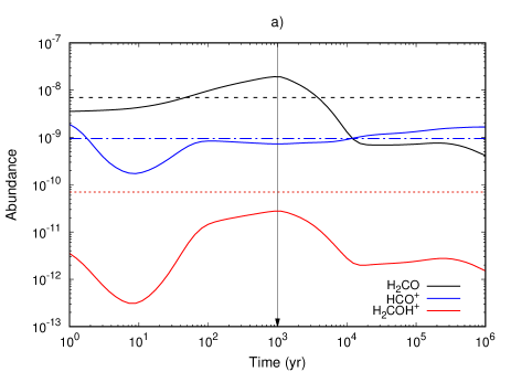
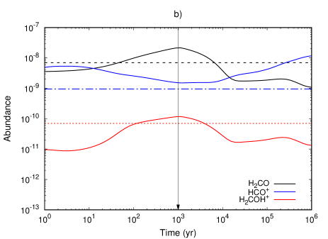
Figure 8: Predicted abundances of H₂CO, HCO⁺ and H₂COH⁺ as a function of time, represented by the black, blue and red solid lines, respectively, obtained from a model with $T$=30 K and $n_{\text{H}_{2}}$=1 $\times$ 10⁶ cm^-3. Panel a) represents a model with the whole chemical network whereas panel b) does not include the major destruction channels of HCO⁺ and H₂COH⁺. The dashed, dash-dotted and dotted horizontal lines indicate the mean fractional abundances observed in G331 for H₂CO, HCO⁺ and H₂COH⁺, respectively. The vertical arrow depicts the abundance peak of H₂CO at $t\thickapprox 10^{3}$ yr.

4.3 Isotopic fractionation

D/H ratios: The ratio was calculated using the neutral isotopologues H₂CO and HDCO, while molecular ions HCO⁺ and DCO⁺ were not used due to the non detection of DCO⁺ in G331. From the LTE and non-LTE analyses of HDCO and H₂CO, respectively, it is reported HDCO/H₂CO $\sim$ 0.02 for a bulk gas with $T<$90 K and, from the D₂CO tentative detection, it was estimated D₂CO/H₂CO $\leq$ 0.009. Roberts & Millar (2007) estimated HDCO/H₂CO $\sim$ 0.01, 0.03, and $<$0.002 in G34.26, G75.78 and G31.41, respectively. In addition, for the G34.26 and G75.78 sources, they also reported D₂CO/H₂CO $<$ 0.001 and $<$0.01, respectively, for gas components within a broad distribution of temperatures ($T<$ 100 K).

The HDCO detection demonstrated clear evidences of deuteration fractionation in G331. In previous studies of G331 conducted with APEX, deuterated species were searched but no conclusive results were obtained (Mendoza et al., 2018; Duronea et al., 2019; Canelo et al., 2021; Santos et al., 2022).

¹²C/¹³C ratios: The H₂CO/H${}_{2}^{13}$CO and HCO⁺/H¹³CO⁺ ratios were estimated in G331 within $\sim$ 14–20. Wilson & Rood (1994) analyzed isotopic carbon ratios from CO and H₂CO reporting values of $\sim$ 20 and 77 for the Galactic center and Local ISM, respectively. Yan et al. (2019) estimated ¹²C/¹³C ratios from formaldehyde. From 112 observations, the transition (1_1,0–1_1,1) of H₂CO was detected in 84 sources and from these 84, H${}_{2}^{13}$CO (1_1,0–1_1,1) was detected in 38 sources (the entire description is in § 2 of Yan et al. 2019). They found ¹²C/¹³C ratio values up to 99 for the source G49.21-0.35, around 32 for G31.41+0.31, and $\sim$ 16–47 for W31.

¹⁶O/¹⁸O and ¹⁸O/¹⁷O ratios: The H₂C¹⁶O/H₂C¹⁸O and HC¹⁶O⁺/HC¹⁸O⁺ ratios provided a rough estimate between $\sim$ 170–250. In order to estimate the ¹⁸O/¹⁷O ratio, from the integrated areas of the lines HC¹⁷O⁺ (2–1) and HC¹⁸O⁺ (2–1), the ratio HC¹⁸O⁺/HC¹⁷O${}^{+}\sim$ 3 is obtained, whose value represents an upper limit compared with the abundance ratio HC¹⁸O⁺/HC¹⁷O${}^{+}\sim$ 1.3, obtained for G331 from the LTE analysis. In the Galactic center and local ISM, Wilson & Rood (1994) obtained ratios of ¹⁶O/¹⁸O $\sim$ 250 and 560, respectively, as well as ¹⁸O/¹⁷O $\sim$ 3.2 for both of them. Persson et al. (2018) claimed the first detection of H₂C¹⁷O and D${}_{2}^{13}$CO, among other isotopologues, in IRAS 16293-2422 B and reported the values H₂C¹⁶O/H₂C¹⁸O$\sim$ 800, H₂C¹⁶O/H₂C¹⁷O$\sim$ 2596 and H₂C¹⁸O/H₂C¹⁷O$\sim$ 3.2.

In summary, we present in Table 5 the isotopic ratios estimated for G331 which are in good agreement compared to the values reported from Giant Molecular Clouds (Orion, Sgr B2) and hot molecular cores as G31.41 and G34.26 (Guelin et al., 1982; Turner, 1990; Mangum et al., 1990; Roberts & Millar, 2007; Neill et al., 2013; Yan et al., 2019).

Table 5: Ratios between the isotopologues of H₂CO and HCO⁺ estimated for G331 which are compared with the values reported in Giant Molecular Clouds (GMCs), i.e., Orion and Sgr (B2), and hot molecular cores (HMCs), i.e., G31.41 and G34.26.

Ratios	G331	GMCs	G31.41	G34.26
Formaldehyde
H${}_{2}^{13}$CO/H2CO	0.05	0.035a	0.03e	0.02e
HDCO/H2CO	0.02	$\leqslant$ 0.005b	$<$ 0.002f	0.01f
D2CO/HDCO	$\lesssim$0.5	0.02c	–	$<$ 0.001f
H2C18O/H2CO	0.004	0.003a	–	–
Formyl cation
HCO+/H13CO+	14	21.2d	–	–
HC18O+/HC17O+	1.3	3.1d	–	–

a)Orion KL compact ridge (Mangum et al., 1990). b) Orion KL Hot Core (Neill et al., 2013). c) Orion KL Compact Ridge (Turner, 1990). d) Sgr B2 (Stark, 1981; Guelin et al., 1982). e) HMCs (Yan et al., 2019). f) HMCs (Roberts & Millar, 2007).

5 Conclusions and perspectives

We have identified isotopologues of formaldehyde, formyl cation and protonated formaldehyde in G331, a hot molecular core and outflow system. The search for those species were carried out using spectral setups collected with the APEX telescope in the frequency range $\sim$ 159–356 GHz. A time dependent chemical model, using the gas grain code Nautilus, was performed to study the chemistry and predict the abundances of H₂CO, HCO⁺ and H₂COH⁺ as a function of time. The conclusions and perspectives are:

• Formaldehyde is an abundant molecule in G331. Several lines of H₂CO, H${}_{2}^{13}$CO, HDCO and H₂C¹⁸O were detected in G331, 35 spectral lines in total. D₂CO was tentatively detected and was used to set an upper threshold for its abundance. From non-LTE calculations, the o- and p-H₂CO spectral lines provided kinetic temperatures between $\sim$ 87–95 K. From the population diagrams assuming the LTE approximation, the spectral lines of H${}_{2}^{13}$CO, HDCO and H₂C¹⁸O provided excitation temperatures of $\sim$ 83, 21 and 31 K. From the estimates of column densities considering a source size of 5″, the ratios H₂CO:H${}_{2}^{13}$CO:HDCO:H₂C¹⁸O$\thickapprox$223:12:4:1 were obtained. The formaldehyde isotopologues can trace different physical conditions, from cold gas to lukewarm temperatures. These results agree with sublimation processes and the active gas-grain chemistry expected in hot molecular cores.

• The formyl cation is also an abundant species in G331. In total, 8 rotational lines of HCO⁺, H¹³CO⁺, HC¹⁸O⁺ and HC¹⁷O⁺ were identified in G331. In contrast with formaldehyde, the ¹⁷O isotopologue, HC¹⁷O⁺, was detected but not the deuterated one, DCO⁺. Assuming the LTE approximation, the population diagram of H¹³CO⁺ provided a temperature and column density $T_{\rm exc}\thickapprox$ 11 K and $N$(H¹³CO⁺) $\thickapprox$ 2.1 $\times$ 10¹⁴ cm^-2, whose values were used to estimate the column densities of HC¹⁸O⁺ and HC¹⁷O⁺. From non-LTE calculations, the spectral lines of HCO⁺ provided $N$(HCO⁺) $\thickapprox 3\times$10¹⁵ cm^-2 assuming a temperature of about 30 K.

• The protonated formaldehyde, H₂COH⁺, should be present under interstellar conditions when H₂CO and HCO⁺ are detected (see Eq. 1). In fact, this cation was also detected through four lines, of which one of them is likely blended with ³⁴SO₂. From the population diagram considering the LTE formalism, it was obtained $T_{\rm exc}\thickapprox$ 25 K and $N$(H₂COH⁺) $\thickapprox$ 1.4 $\times$ 10¹⁴ cm^-2 adopting a source size of 5″. H₂CO and HCO⁺ can produce H₂COH⁺ under interstellar conditions. In addition, these species could play a key role in the formation of complex organic molecules.

• A gas grain chemical model was performed to predict the fractional abundances of H₂CO, HCO⁺ and H₂COH⁺ and to study their evolution. The best model was obtained adopting $T=$30 K and $n_{\text{H}_{2}}=1\times$ 10⁶ cm^-3. In a young molecular stage of $\sim$ 10³ yr, the H₂CO, HCO⁺ and H₂COH⁺ abundances reached comparable values to those derived from the observations, [H₂CO] = (0.2–2) $\times$10^-8, [HCO⁺] = (0.5–4) $\times$10^-9 and [H₂COH⁺] = (0.2–2) $\times$10^-10. The reaction between H₂CO and HCO⁺ is one of the major channels to produce H₂COH⁺. On the other hand, it was noticed that dissociative recombination mechanisms with electrons can rapidly destroy HCO⁺ and H₂COH⁺ affecting their predicted abundances. The results obtained with the chemical modeling of the three molecular species makes us to develop a hypothesis that the evolution stage of G331 is around $10^{3}$ yr. Further studies in G331 should be carried out to confirm this hypothesis.

• From the multi-line analysis of formaldehyde and the formyl cation, new ¹²C/¹³C, H/D, ¹⁶O/¹⁸O and ¹⁸O/¹⁷O ratios were inferred in G331 and agree with the results of other works. In particular, deuterium was observed in formaldehyde but not in the formyl cation, HDCO and DCO⁺, respectively. ¹⁷O was observed in the formyl cation but not in formaldehyde, HC¹⁷O⁺ and H₂C¹⁷O, respectively. In perspective, along with new observational analysis, gas-grain chemical models might shed light on the molecular processes that lead different isotopic ratios.

Appendix A Update of the internal partition functions of the detected isotopologues of formaldehyde

The internal partition functions of the isotopologues of formaldehyde H${}_{2}^{13}$CO, H₂C¹⁸O, HDCO and D₂CO detected in this work have been updated. Since the lists of energies, either experimental or theoretical, of the rovibrational levels for these isotopologues are incomplete for computing the internal partition functions for temperatures up to 500 K, the direct sum expression does not reach the convergence. Therefore, the internal partition functions of the isotopologues of formaldehyde have to be computed using some other tested approximations (Carvajal et al., 2019), e.g., writing it in terms of the product of the rotational contribution ($Q_{\rm rot}(T)$) and the harmonic approximation of the vibrational contribution ($Q_{\rm vib}^{\rm harm}(T)$) (Herzberg, 1991)

$$Q_{\rm rv}(T)\approx Q_{\rm rot}(T)\,Q_{\rm vib}^{\rm harm}(T)~{}~{}.$$ (A1)

where the rotational contribution $Q_{\rm rot}(T)$ is computed as a direct sum (e.g., Herzberg (1991)) because there are enough rotational energies for the typical temperatures of the ISM,

$$Q_{\rm rot}(T)=\sum_{\rm i}g_{\rm ns}^{({\rm i})}\,(2\,J_{\rm i}+1)\,e^{-{E^{({\rm rot})}_{\rm i}\over kT}}~{}~{}.$$ (A2)

$E^{({\rm rot})}_{\rm i}$ represents the energy for the i-th rotational state in the ground vibrational state assuming that uniquely the ground electronic state is populated. The rotational energies of the isotopologues of formaldehyde have been taken from the Cologne Database for Molecular Spectroscopy catalog (CDMS) (Endres et al., 2016) and from JPL (Pickett et al., 1998).

The nuclear spin degeneracy $g_{\rm ns}^{({\rm i})}$ is included in the definition of the rotational contribution of the partition function (Eq. A2) because, in general, the values of $g_{\rm ns}^{({\rm i})}$ can be different depending on the symmetry of the rotational states. In the case of formaldehyde, the isotopologues H${}_{2}^{13}$CO, H₂C¹⁸O, and D₂CO have symmetry ${\cal C}_{2v}(M)$, whose rovibrational states are characterized by the irreducible representations $A_{1}$, $A_{2}$, $B_{1}$ and $B_{2}$, whereas the monodeuterated isotopologue HDCO has symmetry ${\cal C}_{s}(M)$ and its states are labeled with the irreducible representations $A^{\prime}$ and $A^{\prime\prime}$ (Bunker & Jensen, 1989). The labelings of the rotational states of the different isotopologues as well as their nuclear spin statistical weights are given in Table 6.

Although the validity of the approximation (A1) has been proven suitable for the typical ISM temperatures (Carvajal et al., 2019), a new check is carried out comparing the values of the internal partition function of the main isotopologue of formaldehyde from 2.725 K to 500 K with those calculated as a direct sum of a comprehensive data set for the rovibrational energy levels provided by Al-Refaie et al. (2015). In Tab. 7, the values of the harmonic approximation for the vibrational partition function $Q_{\rm vib}^{\rm harm}(T)$ and the internal partition function $Q_{\rm rv}(T)$ (A1) for the main isotopologue are given. $Q_{\rm vib}^{\rm harm}(T)$ is calculated using the experimental fundamental vibrational energies taken from Perrin et al. (2003, 2006) and the rotational partition function is computed from the JPL rotational energies predicted up to J=99 and K_a=25 (Pickett et al., 1998). The uncertainties of the rovibrational partition function (Carvajal et al., 2019) are obtained considering the uncertainties of all the rotational energies provided in the JPL database (Pickett et al., 1998) and the experimental uncertainties of the vibrational fundamental energies (Perrin et al., 2003, 2006). These values are compared with those from CDMS catalog (Endres et al., 2016) and from Al-Refaie et al. (2015). According to the relative differences between the approximated internal partition function (A1) and the one calculated more thoroughly (Al-Refaie et al., 2015), the two results are comparable in the temperature interval from 2.725 K and 500 K. However, the difference with the values provided in the CDMS catalog is of -8.8% at 500 K and of -0.72% at 300 K. Therefore, as the approximation (A1) using a harmonic vibrational partition function is acceptable for the interval of temperature typical for the ISM and improves notably the values of JPL and CDMS catalogs for higher temperatures, this is going to be used for the other isotopologues of formaldehyde.

Tab. 8 evinces the values of the partition function of H${}_{2}^{13}$CO, H₂C¹⁸O, D₂CO, and HDCO calculated in this work. As in Tab. 7, the values of the calculated partition function are compared with those available in CDMS database (Endres et al., 2016). For the case of H${}_{2}^{13}$CO, the values and the uncertainties of $Q_{\rm rv}(T)$ are computed using experimental fundamental vibrational energies (Ng & Tan, 2017; Wohar & Jagodzinski, 1991) for the harmonic partition function and rotational energies up to J=99 and K_a=25 taken from JPL database (Pickett et al., 1998). The highest relative difference between this work and CDMS values is of -0.76% at T=300 K. Therefore, at this temperature is not relevant to incorporate the vibrational contribution to the partition function. Nevertheless, the vibrational contribution is important at T=500 K increasing the rotational partition function about 9%.

For the isotopologue H₂C¹⁸O only the values of the rotational partition function are evinced in Tab. 8. These values and their uncertainties have been calculated using the CDMS rotational data (up to J=54, K_a=16) complemented with those predicted for the excited rotational levels from JPL database (up to J=20, K_a=20) when missing in the CDMS catalog. The vibrational partition function could not be calculated because, as far as we know, there are neither fundamental energies nor excited vibrational energies reported in the literature at all. This hindrance could be overcome providing the vibrational fundamental energies calculated by ab initio or other empirical approaches. Therefore, the partition function in the present work is practically the same reported in CDMS apart from the uncertainties and the new values of the rotational partition function for temperatures from 300 K to 500 K.

The vibrational and the internal partition functions of the double deuterated isotopologue D₂CO are presented in Tab. 8. The vibrational contribution and its uncertainty have been calculated using the available experimental vibrational fundamental bands (Perrin et al., 1998; Lohilahti & Alanko, 2001; Lohilahti et al., 2006). The values and the uncertainties of the rotational partition function are calculated using the CDMS rotational energies (with data up to J=66 and K_a=26) complemented with higher excited rotational energy predictions (up to J=60 and K_a=60) given in JPL database. At T=300 K the difference of the updated internal partition function with CDMS values is around 2.6% and this will be around 20% at T=500 K.

The values and uncertainties of the internal partition function of the monodeuterated isotopologue HDCO as well as the vibrational contribution are also included in Tab. 8. The values of the rotational partition function are calculated using the CDMS rotational energies (up to J=56 and K_a=20) complemented with JPL higher excited rotational energy predictions up to J=90 and K_a=50. Since the CDMS data are more accurate they were substituted in the JPL predictions to have a more accurate internal partition function. The vibrational partition function is computed using the available experimental and calculated fundamental energies (Oka & Morino, 1961; Dangoisse et al., 1978; Ellsworth et al., 2008; Morgan et al., 2018). The experimental uncertainties of the fundamentals $\nu_{1}$, $\nu_{2}$, $\nu_{4}$, and $\nu_{6}$ measured by Dispersed Fluorescence spectroscopy (Ellsworth et al., 2008) are considered as 2 cm^-1 according to the widths of the spectral lines whereas the uncertainties of $\nu_{3}$ and $\nu_{5}$ bands obtained with DVR calculations are assigned with 1.20 cm^-1. By comparing with the CDMS data, the relative difference of the updated internal partition function is 1.5% larger at T=300 K and at least of 14% at T=500 K.

In general, the update of the internal partition functions incorporate the vibrational contribution as well as the uncertainties and new values from 300 K to 500 K for the four isotopologues H${}_{2}^{13}$CO, H₂C¹⁸O, D₂CO, and HDCO. As supplementary material, their rotational, vibrational and rovibrational partition functions are reported up to T=500 K using a 1 K interval. This update of the partition functions could be relevant for the estimate of the abundances of the four isotopologues of formaldehyde.

Table 6: Nuclear spin statistical weights of the isotopologues of formaldehyde H₂CO, H${}_{2}^{13}$CO, H₂C¹⁸O, D₂CO and HDCO associated to the rotational states^a.

Isotopologues	$\Gamma_{\rm rot}$ b	$K_{a}$ c	$K_{c}$ c	$g_{\rm ns}^{({\rm i})}$	Type g
H2CO,H2C18O	$A_{1}$	even	even	1	para
	$A_{2}$	even	odd	1	para
	$B_{1}$	odd	odd	3	ortho
	$B_{2}$	odd	even	3	ortho
H${}_{2}^{13}$CO	$A_{1}$	even	even	2 d	para
	$A_{2}$	even	odd	2 d	para
	$B_{1}$	odd	odd	6 d	ortho
	$B_{2}$	odd	even	6 d	ortho
D2CO	$A_{1}$	even	even	6 e	ortho
	$A_{2}$	even	odd	6 e	ortho
	$B_{1}$	odd	odd	3 e	para
	$B_{2}$	odd	even	3 e	para
HDCO	$A^{\prime}$	—-	even	6 f	—-
	$A^{\prime\prime}$	—-	odd	6 f	—-

^a The nuclear spin degeneracy $g_{\rm ns}^{({\rm i})}$ is computed according to Bunker & Jensen (1989).

^b The symmetry labeling of the rotational states.

^c The rotational states of the asymmetric top, such as formaldehyde, are labeled by the quantum numbers $J_{K_{a},K_{c}}$, where $J$ is the rotational angular momentum and the $K_{a}$ and $K_{c}$ are the projections of the rotational angular momentum along the $a$- and $c$- molecule-fixed axes. In this case, the symmetry of the rotational states is characterized by their even and odd values of $K_{a}$ and $K_{c}$. For the monodeuterated isotopologue, the two symmetries are only characterized by the even and odd values of $K_{c}$.

^d For H${}_{2}^{13}$CO, the nuclear spin degeneracy is also considered in the literature with a ratio 3:1 for the ortho:para states, respectively (see, e.g., Endres et al. (2016)). As a warning in order to avoid wrong results, before using data from a catalog, it should be checked whether the nuclear spin weights agree with the partition function considered.

^e For D₂CO, the nuclear spin degeneracy is also considered in the literature with a ratio 2:1 (ortho:para) (see, e.g., Endres et al. (2016)). Same warning from footnote $d$ should be considered in this case.

^f For the monodeuterated isotopologue, the nuclear spin degeneracy is considered in this paper as 1 because the degeneracy is state independent.

^g Only for the symmetric isotopologues of formaldehyde, this column shows whether the transitions involving these rotational states are either ortho or para.

Table 7: Vibrational and rotational-vibrational partition function of the main isotopologue of formaldehyde (H₂CO). Comparison between the values obtained in the present study and those published before.^a

$T$(K)	$Q_{\rm vib}^{\rm harm}$ b	$Q_{\rm rv}$(Present work)c	$Q$(CDMS)d	$Q$(Al-Refaie et al., 2015)e	Rel. Diff.(%)f
2.725	1.000000	2.0166(0)	2.0166	2.0165	0.00
5.000	1.000000	4.4832(0)	4.4832	4.4833	0.00
9.375	1.000000	13.8009(0)	13.8008	13.8010	0.00
18.750	1.000000	44.6813(0)	44.6812	44.6835	0.00
37.500	1.000000	128.6496(0)	128.6492	128.6581	0.01
75.000	1.000000	361.7207(0)	361.7195	361.7053	0.00
150.000	1.000021	1019.9947(0)	1019.9706	1019.9549	0.00
225.000	1.000996	1874.4927(0)	1872.6221	1874.4679	0.00
300.000	1.007228	2903.8609(0)	2883.0163	2904.1778	0.01
500.000	1.087521	6751.7086(3)	6208.3442	6760.2315	0.13

^a The nuclear spin degeneracy is given in Tab.6.

^b Values of the vibrational partition function computed with the harmonic approximation. For more details, see the text.

^c $Q_{\rm rv}=Q_{\rm rot}(\mbox{\rm direct sum})\,Q_{\rm vib}^{\rm harm}$. An estimate of the uncertainties is given in parentheses in units of the last quoted digits. For more details, see the text.

^d Rotational partition function computed as a direct sum with no vibrational contribution. Their values are reported in CDMS catalog (Endres et al., 2016).

^e Internal partition function computed as the direct sum using a comprehensive set of rovibrational energies up to 18000 cm^-1 and up to J=70 (Al-Refaie et al., 2015).

^f Relative difference of the partition function computed in the present study with respect to the one reported by Al-Refaie et al. (2015).

Table 8: Vibrational and rotational-vibrational partition functions for the isotopologues H${}_{2}^{13}$CO, H₂C¹⁸O, D₂CO and HDCO. Comparison between the values obtained in the present study and those published in CDMS catalog^a.

	H${}_{2}^{13}$CO				H2C18O
$T$(K)	$Q_{\rm vib}^{\rm harm}$ b	$Q_{\rm rv}$(Present work)c	$Q$(CDMS)d	Rel. Diff.(%)e	$Q_{\rm rot}$(Present work)c		$Q$(CDMS)d	Rel. Diff.(%)e
2.725	1.000000	4.1136(0)	4.1136	0.00	2.0944(0)		2.0944	0.00
5.0	1.000000	9.1701(0)	9.1700	0.00	4.6806(0)		4.6805	0.00
9.375	1.000000	28.2638(0)	28.2636	0.00	14.4425(0)		14.4424	0.00
18.75	1.000000	91.5675(0)	91.5672	0.00	46.8159(0)		46.8156	0.00
37.50	1.000000	263.7391(0)	263.7382	0.00	134.8810(0)		134.8805	0.00
75.0	1.000000	741.6749(0)	741.6726	0.00	379.3628(0)		379.3616	0.00
150.0	1.000023	2091.5874(3)	2091.5330	0.00	1069.8884(0)		1069.8850	0.00
225.0	1.001065	3844.176(18)	3840.0722	-0.11	1964.3668(0)		1964.3606	0.00
300.0	1.007605	5957.09(14)	5912.1084	-0.76	3024.3241(1)		3024.3231	0.00
500.0	1.090530	13884.1(19)	—-	—-	6508.862(13)		—-	—-
	D2CO				HDCO
$T$(K)	$Q_{\rm vib}^{\rm harm}$ b	$Q_{\rm rv}$(Present work)c	$Q$(CDMS)d	Rel. Diff.(%)e	$Q_{\rm vib}^{\rm harm}$ b	$Q_{\rm rv}$(Present work)c	$Q$(CDMS)d	Rel. Diff.(%)e
2.725	1.000000	14.984964(0)	14.9850	0.00	1.000000	2.2608(0)	2.2608	0.00
5.000	1.000000	29.703636(0)	29.7036	0.00	1.000000	4.6483(0)	4.6483	0.00
9.375	1.000000	67.339744(0)	67.3395	0.00	1.000000	11.2681(0)	11.2680	0.00
18.750	1.000000	182.210324(0)	182.2098	0.00	1.000000	31.0556(0)	31.0555	0.00
37.500	1.000000	509.265756(0)	509.2641	0.00	1.000000	86.7359(0)	86.7356	0.00
75.000	1.000000	1432.775532(0)	1432.7709	0.00	1.000000	243.8496(0)	243.8488	0.00
150.000	1.000226	4044.511598(0)	4043.5866	0.02	1.000093	688.0292(0)	687.9631	-0.01
225.000	1.005192	7464.6706(1)	7426.0941	-0.52	1.002701	1266.752(29)	1263.3349	-0.27
300.000	1.025736	11729.1102(6)	11434.7820	-2.57	1.015159	1974.73(18)	1945.2333	-1.52
500.000	1.202824	29624.2096(74)	—-	—-	1.138623	4769.8(21)	—-	—-

^a The nuclear spin degeneracy is considered according to Tab. 6.

^b The vibrational partition function is computed with the harmonic approximation. For more details, see the text.

^c $Q_{\rm rv}=Q_{\rm rot}(\mbox{\rm direct sum})\,Q_{\rm vib}^{\rm harm}$. An upward estimate of the uncertainties is given in parentheses in units of the last quoted digits. For more details, see the text. For the isotopologue H₂C¹⁸O, it is presented the rotational partition function because there are neither experimental nor theoretical vibrational levels available in the literature.

^d Rotational partition function computed as a direct sum with no vibrational contribution. Their values are reported in CDMS catalog (Endres et al., 2016). The CDMS partition functions of H${}_{2}^{13}$CO and D₂CO are multiplied by 2 and 3, respectively, to consider the same nuclear spin statistical weight from Tab. 6.

^e Relative difference of the partition function given in the present study with respect to the one reported in CDMS catalog.

References

- Al-Refaie et al. (2015) Al-Refaie, A. F., Yachmenev, A., Tennyson, J., & Yurchenko, S. N. 2015, Monthly Notices of the Royal Astronomical Society, 448, 1704, doi: 10.1093/mnras/stv091
- Araya et al. (2015) Araya, E. D., Olmi, L., Morales Ortiz, J., et al. 2015, ApJS, 221, 10, doi: 10.1088/0067-0049/221/1/10
- Bacmann et al. (2016) Bacmann, A., García-García, E., & Faure, A. 2016, A&A, 588, L8, doi: 10.1051/0004-6361/201628280
- Bacmann et al. (2003) Bacmann, A., Lefloch, B., Ceccarelli, C., et al. 2003, ApJ, 585, L55, doi: 10.1086/374263
- Belitsky et al. (2018) Belitsky, V., Lapkin, I., Fredrixon, M., et al. 2018, A&A, 612, A23, doi: 10.1051/0004-6361/201731458
- Bianchi et al. (2017) Bianchi, E., Codella, C., Ceccarelli, C., et al. 2017, MNRAS, 467, 3011, doi: 10.1093/mnras/stx252
- Blake et al. (1986) Blake, G. A., Sutton, E. C., Masson, C. R., & Phillips, T. G. 1986, ApJS, 60, 357, doi: 10.1086/191090
- Blake et al. (1987) —. 1987, ApJ, 315, 621, doi: 10.1086/165165
- Bronfman et al. (2008) Bronfman, L., Garay, G., Merello, M., et al. 2008, ApJ, 672, 391, doi: 10.1086/522487
- Bunker & Jensen (1989) Bunker, P. R., & Jensen, P. 1989, Molecular Symmetry and Spectroscopy (NRC Research Press, Ottawa)
- Canelo et al. (2021) Canelo, C. M., Bronfman, L., Mendoza, E., et al. 2021, MNRAS, 504, 4428, doi: 10.1093/mnras/stab1163
- Carvajal et al. (2019) Carvajal, M., Favre, C., Kleiner, I., et al. 2019, A&A, 627, A65, doi: 10.1051/0004-6361/201935469
- Ceccarelli et al. (1998) Ceccarelli, C., Castets, A., Loinard, L., Caux, E., & Tielens, A. G. G. M. 1998, A&A, 338, L43
- Chapovsky (2001) Chapovsky, P. 2001, Journal of Molecular Structure, 599, 337 , doi: https://doi.org/10.1016/S0022-2860(01)00854-7
- Clouthier & Ramsay (1983) Clouthier, D. J., & Ramsay, D. A. 1983, Annual Review of Physical Chemistry, 34, 31, doi: 10.1146/annurev.pc.34.100183.000335
- Crockett et al. (2014) Crockett, N. R., Bergin, E. A., Neill, J. L., et al. 2014, ApJ, 781, 114, doi: 10.1088/0004-637X/781/2/114
- Dangoisse et al. (1978) Dangoisse, D., Willemot, E., & Bellet, J. 1978, Journal of Molecular Spectroscopy, 71, 414, doi: https://doi.org/10.1016/0022-2852(78)90094-2
- Dumke & Mac-Auliffe (2010) Dumke, M., & Mac-Auliffe, F. 2010, in Society of Photo-Optical Instrumentation Engineers (SPIE) Conference Series, Vol. 7737, Proc. SPIE, 77371J, doi: 10.1117/12.858020
- Duronea et al. (2019) Duronea, N. U., Bronfman, L., Mendoza, E., et al. 2019, MNRAS, 489, 1519, doi: 10.1093/mnras/stz2087
- Eckhardt et al. (2018) Eckhardt, A. K., Linden, M. M., Wende, R. C., Bernhardt, B., & Schreiner, P. R. 2018, Nature Chemistry, 10, 1141, doi: 10.1038/s41557-018-0128-2
- Ellsworth et al. (2008) Ellsworth, K. K., Lajiness, B. D., Lajiness, J. P., & Polik, W. F. 2008, Journal of Molecular Spectroscopy, 252, 205, doi: https://doi.org/10.1016/j.jms.2008.09.003
- Endres et al. (2016) Endres, C. P., Schlemmer, S., Schilke, P., Stutzki, J., & Müller, H. S. P. 2016, Journal of Molecular Spectroscopy, 327, 95, doi: 10.1016/j.jms.2016.03.005
- Féraud et al. (2019) Féraud, G., Bertin, M., Romanzin, C., et al. 2019, ACS Earth and Space Chemistry, 3, 1135, doi: 10.1021/acsearthspacechem.9b00057
- Ferus et al. (2019) Ferus, M., Pietrucci, F., Saitta, A. M., et al. 2019, A&A, 626, A52, doi: 10.1051/0004-6361/201935435
- Flower (1999) Flower, D. R. 1999, MNRAS, 305, 651, doi: 10.1046/j.1365-8711.1999.02451.x
- Ford et al. (2004) Ford, K. E. S., Neufeld, D. A., Schilke, P., & Melnick, G. J. 2004, ApJ, 614, 990, doi: 10.1086/423886
- Fuente et al. (2014) Fuente, A., Cernicharo, J., Caselli, P., et al. 2014, A&A, 568, A65, doi: 10.1051/0004-6361/201323074
- Gardner & Whiteoak (1974) Gardner, F. F., & Whiteoak, J. B. 1974, Nature, 247, 526, doi: 10.1038/247526a0
- Ghesquière et al. (2015) Ghesquière, P., Mineva, T., Talbi, D., et al. 2015, Physical Chemistry Chemical Physics (Incorporating Faraday Transactions), 17, 11455, doi: 10.1039/C5CP00558B
- Goldsmith & Langer (1999) Goldsmith, P. F., & Langer, W. D. 1999, ApJ, 517, 209, doi: 10.1086/307195
- Guelin et al. (1982) Guelin, M., Cernicharo, J., & Linke, R. A. 1982, ApJ, 263, L89, doi: 10.1086/183930
- Güsten et al. (2006) Güsten, R., Nyman, L. Å., Schilke, P., et al. 2006, A&A, 454, L13, doi: 10.1051/0004-6361:20065420
- Guzmán et al. (2013) Guzmán, V. V., Goicoechea, J. R., Pety, J., et al. 2013, A&A, 560, A73, doi: 10.1051/0004-6361/201322460
- Halfen et al. (2006) Halfen, D. T., Apponi, A. J., Woolf, N., Polt, R., & Ziurys, L. M. 2006, ApJ, 639, 237, doi: 10.1086/499225
- Hamberg et al. (2007) Hamberg, M., Geppert, W. D., Thomas, R. D., et al. 2007, Molecular Physics, 105, 899, doi: 10.1080/00268970701206642
- Hasegawa & Herbst (1993) Hasegawa, T. I., & Herbst, E. 1993, MNRAS, 263, 589, doi: 10.1093/mnras/263.3.589
- Helmich & van Dishoeck (1997) Helmich, F. P., & van Dishoeck, E. F. 1997, A&AS, 124, 205, doi: 10.1051/aas:1997357
- Hervías-Caimapo et al. (2019) Hervías-Caimapo, C., Merello, M., Bronfman, L., et al. 2019, ApJ, 872, 200, doi: 10.3847/1538-4357/aaf9ac
- Herzberg (1991) Herzberg, G. 1991, Spectra and Molecular Structure: II. Infrared and Raman Spectra of Polyatomic Molecules (Krieger Pub. Co., Malabar, Florida)
- Horn et al. (2004) Horn, A., Møllendal, H., Sekiguchi, O., et al. 2004, ApJ, 611, 605, doi: 10.1086/422137
- Jewell et al. (1989) Jewell, P. R., Hollis, J. M., Lovas, F. J., & Snyder, L. E. 1989, ApJS, 70, 833, doi: 10.1086/191359
- Kalvāns (2021) Kalvāns, J. 2021, ApJ, 910, 54, doi: 10.3847/1538-4357/abe30d
- Lacy et al. (1994) Lacy, J. H., Knacke, R., Geballe, T. R., & Tokunaga, A. T. 1994, ApJ, 428, L69, doi: 10.1086/187395
- Layssac et al. (2020) Layssac, Y., Gutiérrez-Quintanilla, A., Chiavassa, T., & Duvernay, F. 2020, Monthly Notices of the Royal Astronomical Society, 496, 5292, doi: 10.1093/mnras/staa1875
- Lohilahti & Alanko (2001) Lohilahti, J., & Alanko, S. 2001, Journal of Molecular Spectroscopy, 205, 248, doi: https://doi.org/10.1006/jmsp.2000.8256
- Lohilahti et al. (2006) Lohilahti, J., Ulenikov, O., Bekhtereva, E., Alanko, S., & Anttila, R. 2006, Journal of Molecular Structure, 780-781, 182, doi: https://doi.org/10.1016/j.molstruc.2005.05.055
- Loren (1984) Loren, R. B. 1984, Tech. Rep. AST 8116403-1 June 1984
- Mangum & Shirley (2015) Mangum, J. G., & Shirley, Y. L. 2015, PASP, 127, 266, doi: 10.1086/680323
- Mangum et al. (1990) Mangum, J. G., Wootten, A., Loren, R. B., & Wadiak, E. J. 1990, ApJ, 348, 542, doi: 10.1086/168262
- Maret et al. (2011) Maret, S., Hily-Blant, P., Pety, J., Bardeau, S., & Reynier, E. 2011, A&A, 526, A47, doi: 10.1051/0004-6361/201015487
- Maret et al. (2004) Maret, S., Ceccarelli, C., Caux, E., et al. 2004, A&A, 416, 577, doi: 10.1051/0004-6361:20034157
- Martín-Doménech et al. (2019) Martín-Doménech, R., Bergner, J. B., Öberg, K. I., & Jørgensen, J. K. 2019, ApJ, 880, 130, doi: 10.3847/1538-4357/ab2a08
- Meier et al. (1993) Meier, R., Eberhardt, P., Krankowsky, D., & Hodges, R. R. 1993, A&A, 277, 677
- Mendoza et al. (2018) Mendoza, E., Bronfman, L., Duronea, N. U., et al. 2018, ApJ, 853, 152, doi: 10.3847/1538-4357/aaa1ec
- Merello et al. (2013) Merello, M., Bronfman, L., Garay, G., et al. 2013, ApJ, 774, L7, doi: 10.1088/2041-8205/774/1/L7
- Morgan et al. (2018) Morgan, W. J., Matthews, D. A., Ringholm, M., et al. 2018, Journal of Chemical Theory and Computation, 14, 1333, doi: 10.1021/acs.jctc.7b01138
- Mosley et al. (2012) Mosley, J. D., Cheng, T. C., & Duncan, M. A. 2012, in 67th International Symposium on Molecular Spectroscopy, MG07
- Motte et al. (2018) Motte, F., Bontemps, S., & Louvet, F. 2018, ARA&A, 56, 41, doi: 10.1146/annurev-astro-091916-055235
- Muders et al. (2006) Muders, D., Hafok, H., Wyrowski, F., et al. 2006, A&A, 454, L25, doi: 10.1051/0004-6361:20065359
- Müller & Lewen (2017) Müller, H. S. P., & Lewen, F. 2017, Journal of Molecular Spectroscopy, 331, 28, doi: 10.1016/j.jms.2016.10.004
- Neill et al. (2013) Neill, J. L., Crockett, N. R., Bergin, E. A., Pearson, J. C., & Xu, L.-H. 2013, ApJ, 777, 85, doi: 10.1088/0004-637X/777/2/85
- Ng & Tan (2017) Ng, L., & Tan, T. 2017, Journal of Molecular Spectroscopy, 331, 82, doi: https://doi.org/10.1016/j.jms.2016.12.004
- Ohishi et al. (1996) Ohishi, M., Ishikawa, S.-I., Amano, T., et al. 1996, ApJ, 471, L61, doi: 10.1086/310325
- Oka & Morino (1961) Oka, T., & Morino, Y. 1961, Journal of the Physical Society of Japan, 16, 1235, doi: 10.1143/JPSJ.16.1235
- Osterbrock (1962) Osterbrock, D. E. 1962, ApJ, 136, 359, doi: 10.1086/147388
- Pagani et al. (2013) Pagani, L., Lesaffre, P., Jorfi, M., et al. 2013, A&A, 551, A38, doi: 10.1051/0004-6361/201117161
- Paiva et al. (2023) Paiva, M. A. M., Pilling, S., Mendoza, E., Galvão, B. R. L., & De Abreu, H. A. 2023, MNRAS, 519, 2518, doi: 10.1093/mnras/stac3679
- Pegues et al. (2020) Pegues, J., Öberg, K. I., Bergner, J. B., et al. 2020, ApJ, 890, 142, doi: 10.3847/1538-4357/ab64d9
- Perrin et al. (1998) Perrin, A., Flaud, J.-M., Predoi-Cross, A., et al. 1998, Journal of Molecular Spectroscopy, 187, 61, doi: https://doi.org/10.1006/jmsp.1997.7469
- Perrin et al. (2003) Perrin, A., Keller, F., & Flaud, J.-M. 2003, Journal of Molecular Spectroscopy, 221, 192, doi: https://doi.org/10.1016/S0022-2852(03)00207-8
- Perrin et al. (2006) Perrin, A., Valentin, A., & Daumont, L. 2006, Journal of Molecular Structure, 780-781, 28, doi: https://doi.org/10.1016/j.molstruc.2005.03.052
- Persson et al. (2018) Persson, M. V., Jørgensen, J. K., Müller, H. S. P., et al. 2018, A&A, 610, A54, doi: 10.1051/0004-6361/201731684
- Pickett et al. (1998) Pickett, H. M., Poynter, R. L., Cohen, E. A., et al. 1998, J. Quant. Spec. Radiat. Transf., 60, 883, doi: 10.1016/S0022-4073(98)00091-0
- Pratap et al. (1994) Pratap, P., Menten, K. M., & Snyder, L. E. 1994, ApJ, 430, L129, doi: 10.1086/187455
- Quénard et al. (2017) Quénard, D., Bottinelli, S., & Caux, E. 2017, MNRAS, 468, 685, doi: 10.1093/mnras/stx404
- Reboussin et al. (2014) Reboussin, L., Wakelam, V., Guilloteau, S., & Hersant, F. 2014, MNRAS, 440, 3557, doi: 10.1093/mnras/stu462
- Roberts & Millar (2007) Roberts, H., & Millar, T. J. 2007, A&A, 471, 849, doi: 10.1051/0004-6361:20066608
- Roueff et al. (2021) Roueff, A., Gerin, M., Gratier, P., et al. 2021, A&A, 645, A26, doi: 10.1051/0004-6361/202037776
- Ruaud et al. (2015) Ruaud, M., Loison, J. C., Hickson, K. M., et al. 2015, MNRAS, 447, 4004, doi: 10.1093/mnras/stu2709
- Ruaud et al. (2016) Ruaud, M., Wakelam, V., & Hersant, F. 2016, MNRAS, 459, 3756, doi: 10.1093/mnras/stw887
- Sahu et al. (2018) Sahu, D., Minh, Y. C., Lee, C.-F., et al. 2018, MNRAS, 475, 5322, doi: 10.1093/mnras/sty190
- Sánchez-Monge et al. (2013) Sánchez-Monge, Á., López-Sepulcre, A., Cesaroni, R., et al. 2013, A&A, 557, A94, doi: 10.1051/0004-6361/201321589
- Santos et al. (2022) Santos, J. C., Bronfman, L., Mendoza, E., et al. 2022, ApJ, 925, 3, doi: 10.3847/1538-4357/ac36cc
- Schöier et al. (2002) Schöier, F. L., Jørgensen, J. K., van Dishoeck, E. F., & Blake, G. A. 2002, A&A, 390, 1001, doi: 10.1051/0004-6361:20020756
- Schutte et al. (1996) Schutte, W. A., Gerakines, P. A., Geballe, T. R., van Dishoeck, E. F., & Greenberg, J. M. 1996, A&A, 309, 633
- Semenov et al. (2010) Semenov, D., Hersant, F., Wakelam, V., et al. 2010, A&A, 522, A42, doi: 10.1051/0004-6361/201015149
- Shimonishi et al. (2016) Shimonishi, T., Onaka, T., Kawamura, A., & Aikawa, Y. 2016, ApJ, 827, 72, doi: 10.3847/0004-637X/827/1/72
- Singh et al. (2022) Singh, S. K., Fabian Kleimeier, N., Eckhardt, A. K., & Kaiser, R. I. 2022, ApJ, 941, 103, doi: 10.3847/1538-4357/ac8c92
- Snyder et al. (1969) Snyder, L. E., Buhl, D., Zuckerman, B., & Palmer, P. 1969, Phys. Rev. Lett., 22, 679, doi: 10.1103/PhysRevLett.22.679
- Song & Kästner (2017) Song, L., & Kästner, J. 2017, ApJ, 850, 118, doi: 10.3847/1538-4357/aa943e
- Stark (1981) Stark, A. A. 1981, ApJ, 245, 99, doi: 10.1086/158789
- Sutton et al. (1995) Sutton, E. C., Peng, R., Danchi, W. C., et al. 1995, ApJS, 97, 455, doi: 10.1086/192147
- Tang et al. (2021) Tang, X. D., Henkel, C., Menten, K. M., et al. 2021, A&A, 655, A12, doi: 10.1051/0004-6361/202141804
- Taniguchi et al. (2020) Taniguchi, K., Guzmán, A. E., Majumdar, L., Saito, M., & Tokuda, K. 2020, ApJ, 898, 54, doi: 10.3847/1538-4357/ab994d
- Taniguchi et al. (2018) Taniguchi, K., Saito, M., Majumdar, L., et al. 2018, ApJ, 866, 150, doi: 10.3847/1538-4357/aade97
- Tanner et al. (1979) Tanner, S. D., Mackay, G. I., & Bohme, D. K. 1979, Canadian Journal of Chemistry, 57, 2350, doi: 10.1139/v79-378
- Troscompt et al. (2009) Troscompt, N., Faure, A., Wiesenfeld, L., Ceccarelli, C., & Valiron, P. 2009, A&A, 493, 687, doi: 10.1051/0004-6361:200810712
- Tsuge et al. (2020) Tsuge, M., Hidaka, H., Kouchi, A., & Watanabe, N. 2020, ApJ, 900, 187, doi: 10.3847/1538-4357/abab9b
- Turner (1990) Turner, B. E. 1990, ApJ, 362, L29, doi: 10.1086/185840
- van der Tak et al. (2007) van der Tak, F. F. S., Black, J. H., Schöier, F. L., Jansen, D. J., & van Dishoeck, E. F. 2007, A&A, 468, 627, doi: 10.1051/0004-6361:20066820
- Vassilev et al. (2008) Vassilev, V., Meledin, D., Lapkin, I., et al. 2008, A&A, 490, 1157, doi: 10.1051/0004-6361:200810459
- Vastel et al. (2015) Vastel, C., Bottinelli, S., Caux, E., Glorian, J. M., & Boiziot, M. 2015, in SF2A-2015: Proceedings of the Annual meeting of the French Society of Astronomy and Astrophysics, 313–316
- Vidal & Wakelam (2018) Vidal, T. H. G., & Wakelam, V. 2018, MNRAS, 474, 5575, doi: 10.1093/mnras/stx3113
- Wakelam et al. (2015) Wakelam, V., Loison, J. C., Herbst, E., et al. 2015, ApJS, 217, 20, doi: 10.1088/0067-0049/217/2/20
- Watanabe et al. (2003) Watanabe, N., Shiraki, T., & Kouchi, A. 2003, ApJ, 588, L121, doi: 10.1086/375634
- Wiesenfeld & Faure (2013) Wiesenfeld, L., & Faure, A. 2013, MNRAS, 432, 2573, doi: 10.1093/mnras/stt616
- Wilson & Rood (1994) Wilson, T. L., & Rood, R. 1994, ARA&A, 32, 191, doi: 10.1146/annurev.aa.32.090194.001203
- Wohar & Jagodzinski (1991) Wohar, M. M., & Jagodzinski, P. W. 1991, Journal of Molecular Spectroscopy, 148, 13, doi: https://doi.org/10.1016/0022-2852(91)90030-E
- Woods et al. (2012) Woods, P. M., Kelly, G., Viti, S., et al. 2012, ApJ, 750, 19, doi: 10.1088/0004-637X/750/1/19
- Woon & Herbst (2009) Woon, D. E., & Herbst, E. 2009, ApJS, 185, 273, doi: 10.1088/0067-0049/185/2/273
- Wootten et al. (1984) Wootten, A., Loren, R. B., & Bally, J. 1984, ApJ, 277, 189, doi: 10.1086/161681
- Yan et al. (2019) Yan, Y. T., Zhang, J. S., Henkel, C., et al. 2019, ApJ, 877, 154, doi: 10.3847/1538-4357/ab17d6
- Yu et al. (2018) Yu, N.-P., Xu, J.-L., Wang, J.-J., & Liu, X.-L. 2018, ApJ, 865, 135, doi: 10.3847/1538-4357/aadb94
- Zapata et al. (2011) Zapata, L. A., Schmid-Burgk, J., & Menten, K. M. 2011, A&A, 529, A24, doi: 10.1051/0004-6361/201014423