Chiral active matter in external potentials
Abstract
We investigate the interplay between chirality and confinement induced by the presence of an external potential. For potentials having radial symmetry, the circular character of the trajectories induced by the chiral motion reduces the spatial fluctuations of the particle, thus providing an extra effective confining mechanism, that can be interpreted as a lowering of the effective temperature. In the case of non-radial potentials, for instance, with an elliptic shape, chirality displays a richer scenario. Indeed, the chirality can break the parity symmetry of the potential that is always fullfilled in the non-chiral system. The probability distribution displays a strong non-Maxwell-Boltzmann shape that emerges in cross-correlations between the two Cartesian components of the position, that vanishes in the absence of chirality or when radial symmetry of the potential is restored. These results are obtained by considering two popular models in active matter, i.e. chiral Active Brownian particles and chiral active Ornstein-Uhlenbeck particles.
I Introduction
Active matter, encompassing a wide range of self-propelled entities, has emerged as a fascinating field of study in soft matter and non-equilibrium statistical physics Marchetti et al. (2013); Bechinger et al. (2016). Typical active systems are artificial particles, such as active colloids, active granular particles, and drones, but also living systems with biological origins, such as bacteria, sperms, and several animals. These systems usually self-propel by virtue of internal mechanisms that convert energy to produce a net motion, through chemical reactions, cilia, flagella, and internal motors, to mention a few examples.
In several cases, the self-propelled motion is characterized by an almost straight path and a fluctuating orientation that changes stochastically without a preferential direction. This motion is induced by the breaking of the translational symmetry at the single-particle level in the body or in the swimming and running mechanism that induces a net polarity in the particle. The physical or biological systems displaying this motion are classified as linear particles or swimmers. This is the standard scenario for several bacteria, such as E. Coli, active colloids, such as Janus particles, or polar active granular particles. However, in nature, several active systems show trajectories systematically rotating clockwise or counterclockwise, the so-called chiral or circular self-propelled particles Löwen (2016).
The concept of chirality or handedness was introduced by Lord Kelvin more than one century ago in reference to the circular (helical) motion produced by solid bodies with asymmetric shapes in two (three) dimensions. Nowadays, chirality has been renewed in the field of active matter Liebchen and Levis (2022), being observed for instance in proteins Loose and Mitchison (2014), bacteria DiLuzio et al. (2005); Lauga et al. (2006) and sperms Riedel et al. (2005) moving on a two-dimensional planar substrate, and L-shape artificial microswimmers Kümmel et al. (2013). In addition, even spherical (non-chiral) particles can show circular (chiral) trajectories due to asymmetry in their self-propulsion mechanism, as occurs in colloidal propellers in a magnetic or electrical field Zhang et al. (2020), and cholesteric droplets Carenza et al. (2019). In addition, granular systems such as spinners Workamp et al. (2018); Scholz et al. (2021) and Hexbug particles driven by light Siebers et al. (2023) usually display chiral motion.
Being ubiquitous in nature, the interest in chiral active matter is recently showing exponential growth in time, in different contexts ranging from the statistical properties of single-particles to collective phenomena displayed by interacting systems. Through the introduction of simple models, the single-particle chiral active motion has been explicitly explored Wittkowski and Löwen (2012); Kümmel et al. (2013) with a focus on the mean-square displacement Van Teeffelen and Löwen (2008); Sevilla (2016), in a viscoelastic medium Sprenger et al. (2022), in the presence of pillars Van Roon et al. (2022) or sinusoidal channels Ao et al. (2015). In channel geometries, chirality is also responsible for the reduction of the accumulation near boundaries typical of active systems and for the formation of surface currents Caprini and Marconi (2019); Fazli and Naji (2021). In the case of interacting systems, chirality is able to suppress the clustering typical of active particles Ma and Ni (2022); Semwal et al. (2022); Sesé-Sansa et al. (2022); Bickmann et al. (2022) but induces novel phenomena, such as emergent vortices induced by the chirality Liao and Klapp (2018, 2021) or a global traveling wave in the presence of a chemotactic alignment Liebchen et al. (2016). Chiral active particles exhibit fascinating phenomena also in the presence of alignment interactions giving rise to pattern formation Liebchen and Levis (2017); Negi et al. (2022) consisting of rotating macro-droplets Levis and Liebchen (2018), chiral self-recognition Arora et al. (2021), dynamical frustration Huang et al. (2020), and chimera states Kruk et al. (2020). In addition, chirality appears as a fundamental ingredient to observe the hyper-uniform phase Lei et al. (2019); Huang et al. (2021) in active matter as well as emerging odd properties Fruchart et al. (2023); Muzzeddu et al. (2022) for instance in the viscosity Banerjee et al. (2017); Lou et al. (2022); Yang et al. (2021); Lou et al. (2022), elasticity Scheibner et al. (2020), and mobility Poggioli and Limmer (2023). Recently, the circular motion has been also investigated in the framework of active glasses where it gives rise to a novel oscillatory caging effect entirely due to the chirality Debets et al. (2023).
Chirality could play a fundamental role in several applications due to their emerging properties, such as sorting Mijalkov and Volpe (2013); Chen and Ai (2015); Su et al. (2019); Xu et al. (2022) and synchronization Levis et al. (2019); Samatas and Lintuvuori (2023). For instance, chiral microswimmers can be sorted according to their swimming properties by employing patterned microchannels with a specific chirality Mijalkov and Volpe (2013). Chirality is also at the basis of the ratcheting mechanism observed in an array of obstacles Reichhardt and Reichhardt (2013) even leading to translation at fixed angles with respect to the substrate periodicity due to a periodic potential Nourhani et al. (2015). Moreover, binary mixtures of passive and active chiral particles, as well as mixtures of chiral particles with opposite chiralities show demixing Ai et al. (2015, 2018); Reichhardt and Reichhardt (2019); Levis and Liebchen (2019). Spontaneous demixing has been also observed experimentally in a system of active granular particles, the so-called spinners that are self-propelled because of the asymmetry of internal components of their bodies Scholz et al. (2018).
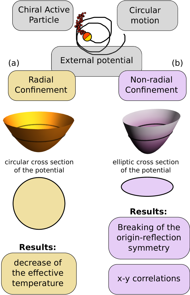
Despite the recent attention on chiral active matter, the interplay between chirality and external confinement due to an external potential has been less investigated Jahanshahi et al. (2017) to the best of our knowledge. Here, we focus on active chiral particles in a radial (circular) and non-radial (elliptic) potential, exploiting the influence of circular motion on the properties of the system. In particular, we perform a numerical and analytical study based on two popular models in active matter, i.e. the chiral active Brownian particles and chiral active Ornstein-Uhlenbeck particles. We anticipate that for a radial potential, the chirality induces only an increasing confinement in the particle’s dynamics, effectively reducing the fluctuations of the systems and, thus its effective temperature (Fig. 1 (a)). In contrast, in the case of non-radial potential, the chirality is able to break the parity symmetry of an elliptic potential. This is reflected, for instance, in the occurrence of strong correlations between different spatial components of the system (Fig. 1 (b)). This effect is uniquely based on the interplay between chirality and spatial asymmetry of the potential.
The paper is structured as follows: in Sec. II, we introduce and discuss the models, i.e. chiral active Brownian particles and chiral active Ornstein-Uhlenbeck particles, employed to perform the numerical and analytical study. The dynamics in the radial and non-radial potentials are analyzed in Sec. III and Sec. IV, respectively. We summarize the results and report a conclusive discussion in the final section V. Finally, for the sake of completeness but also to render the presentation lighter, we reported in an appendix the derivation of the Fokker-Planck equation governing the evolution of the probability distribution function of the chiral active model together with a pair of simple illustrative cases.
II Model
Active particles in the overdamped regime are described by the following dynamics for the particle position :
| (1) |
where is a Brownian white noise with unit variance and zero average accounting for the random collisions with the particle of the solvent. The coefficient is the friction coefficient due to the solvent, while is the translational diffusion coefficient of the system. The term is the external force due to a potential , such that . The last force term in Eq. (1), namely , known as active force, describes at a coarse-grained level the chemical, biological or physical mechanism responsible for the self-propulsion. The constant provides a velocity scale to the dynamics and it is often referred to in the literature as swim velocity, while the vector is a stochastic process with unit variance whose properties and dynamics determine the active model considered. is an additional degree of freedom that is absent for equilibrium systems where . Despite the generality of Eq. (1), for simplicity, we restrict ourselves to two spatial dimensions.
II.1 Chiral active Brownian particles (ABPs).
In the ABP dynamics Buttinoni et al. (2013); Solon et al. (2015); Shaebani et al. (2020); Caporusso et al. (2020); Caprini and Löwen (2023) independently of the chirality, the term is a unit vector, such that , usually associated with the orientation of the active particle. Since the modulus of is unitary, the dynamics of can be conveniently expressed in polar coordinates. In this representation, , where is the orientational angle of the active particle that evolves as a simple diffusive process:
| (2) |
where is a white noise with unit variance and zero average and the typical time can be identified with the persistence time induced by the rotational diffusion coefficient .
In the ABP dynamics, the chirality is introduced by adding an angular drift in Eq. (2), which breaks the rotational symmetry of the active force dynamics and induces a preferential rotation of the vector in the clockwise or counterclockwise direction depending on the sign of . As a consequence, the single-particle trajectories of a chiral ABP tend to be circular. The value of determines the strength of chirality: the larger , the smaller the typical radius of the circular trajectories of a single particle, given by .
II.2 Chiral active Ornstein-Uhlenbeck particles (AOUPs).
In the AOUP dynamics Szamel (2014); Martin et al. (2021); Maggi et al. (2015); Wittmann et al. (2018); Caprini et al. (2019); Keta et al. (2022, 2023), is described by a two-dimensional Ornstein-Uhlenbeck process that allows both the modulus and the orientation to fluctuate with related amplitudes Caprini et al. (2022). The AOUP distribution is a two-dimensional Gaussian such that each component fluctuates around a vanishing mean value with unit variance. The resulting dynamics of the vector reads:
| (3) |
where is a two-dimensional vector of white noises with uncorrelated components having unitary variance and zero average. Here, represents the persistence time of the particle trajectory, i.e. the time that the particle, in the absence of angular drift, spends moving in the same direction before a reorientation of the active force. In the AOUP model the diffusion coefficient due to the active force is obtained form the relation , which allows a simple comparison between AOUP and ABP models Caprini et al. (2022, 2019).
In the AOUP dynamics, the chirality is included by adding the force , where is the direction orthogonal to the plane of motion and the parameter quantifies the chirality of the particle Caprini and Marconi (2019). Such a force is always directed in the plane of motion, normal to , and is orthogonal to , so that it rotates the self-propulsion vector in the clockwise or counterclockwise direction depending on the sign of . Similarly to the chiral ABP model, the chiral AOUP dynamics displays circular trajectories. However, in contrast with the ABP dynamics, the typical circles observed by an AOUP are characterized by a fluctuating radius, that on average is equal to the one of the ABP and . It is worth noting that the chiral term in the AOUP dynamics is totally equivalent to the chiral term in the ABP dynamics. Indeed, the constant force in polar coordinate affects only the dynamics of the polar angle through a constant term equivalent to the driving angular velocity written in Eq. (2).
II.3 Relation between chiral AOUPs and chiral ABPs.
Despite the AOUP and ABP dynamics are different, both are usually employed to describe active particles and display similarities so that AOUP has been often employed to derive analytical predictions suitable to describe ABP numerical results. The reason of this agreement lies in the fact that the two-time self-correlations of of the two models are identical with an approprate choice of parameters Farage et al. (2015); Caprini et al. (2022); Caprini and Marconi (2019). For both cases, we find
| (4) |
It is worth noting that, in Eq. (4), the chirality affects the shape of the autocorrelation by inducing oscillations.
Despite ABP and AOUP have different dynamics and are characterized by different steady-state distributions, such dynamical properties are at the basis of a plethora of similar phenomena observed for a single particle but also for interacting systems. A comparison between the two models has been established for a single non-chiral active particle and a non-chiral active particle in a harmonic potential, while, more generally, the relation between the two models has been deepened in Ref. Caprini et al. (2022). However, the effect of chirality in the two models confined in an external potential has been poorly investigated in the literature.
III Chiral active particle in a radial potential
We start by considering chiral active particles confined by a simple harmonic potential in two dimensions, , that exerts a linear force on the particle directed towards the origin.
Both in chiral ABP and chiral AOUP simulations, it is convenient to rescale time by the persistence time and the position by the persistence length . In this way, the chirality can be tuned by changing the dimensionless parameter , which we call reduced chirality. The other dimensionless parameters of the simulations are the reduced stiffness of the potential and the ratio between passive and active diffusion coefficients, . For simplicity, we set and eliminate . Indeed, the thermal noise is orders of magnitudes smaller than the diffusion due to the active force in several experimental systems Bechinger et al. (2016). Finally, we set . The effect of this parameter has been explored in the AOUP case analytically Szamel (2014), and in the ABP case numerically Caprini et al. (2022) and experimentally Buttinoni et al. (2022) by considering an active Janus particle in an optical tweezer. Here, we focus on the role of reduced chirality, .
Active particles in radial potentials Takatori et al. (2016); Dauchot and Démery (2019); Caprini et al. (2019); Hennes et al. (2014); Rana et al. (2019); Marini Bettolo Marconi et al. (2017); Baldovin et al. (2022) have been widely investigated in the absence of chirality for which we summarize the results: the AOUP dynamics in a harmonic potential can be solved exactly Szamel (2014); Das et al. (2018); Woillez et al. (2020); Caprini and Marini Bettolo Marconi (2021); Nguyen et al. (2021), being fully linear, and is described by a multivariate Gaussian distribution in and . As a consequence, the density of the system is still Gaussian and the active force affects the distribution by changing its effective temperature only Szamel (2014); Fodor et al. (2016); Maggi et al. (2017); Caprini et al. (2022). The ABP dynamics in harmonic potential has been exactly solved only recently Malakar et al. (2020); Caraglio and Franosch (2022) and leads to a more intriguing scenario Pototsky and Stark (2012); Basu et al. (2019). While in the small persistence regime, (small or large ), the density is Gaussian Caprini et al. (2022) and similar to the one of the AOUP, in the large persistence regime, ABPs accumulate far from the potential minimum, as confirmed experimentally by active colloids Takatori et al. (2016); Buttinoni et al. (2022), roughly at the distance where the active force balances the potential force, i.e. at . As a result, the two-dimensional density in the plane of motion is characterized by a Mexican-hat shape while the density, projected onto a single coordinate, displays bimodality. The results observed in the ABP are reminiscent to those originally obtained of considering Run&Tumble particles Tailleur and Cates (2009); Solon et al. (2015); Smith et al. (2022).
III.1 Spatial distribution
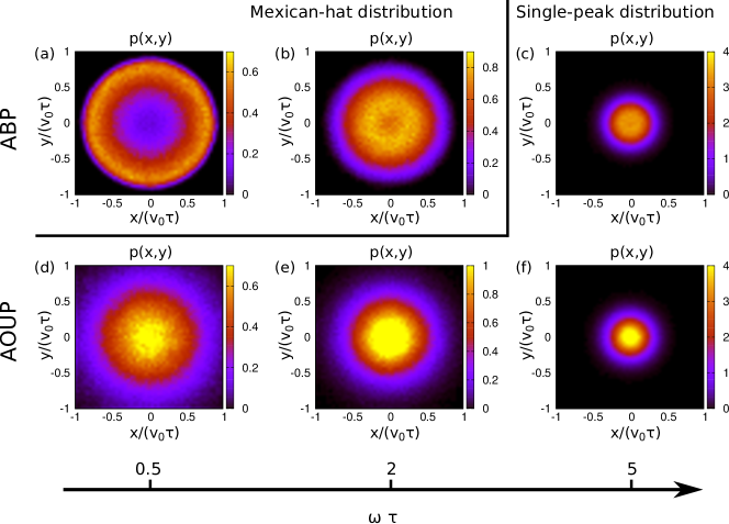
To investigate the role of chirality, we plot the probability distribution in the plane of motion for three representative values of the reduced chirality, . This analysis is performed both for the ABP (Fig. 2 (a)-(c) ) and AOUP (Fig. 2 (d)-(f)) models.
In the chiral AOUP case, the system is linear and, as a consequence, is a Gaussian centered at the origin in both spatial directions, independently of the value of . The increase of the chirality induces a stronger confinement of the particle as if the potential was stiffer or the dynamics governed by a lower effective temperature. Indeed, the system is described by the following
| (5) |
with effective temperature (in units of Boltzmann constant, )
| (6) |
The theoretical results (5) and (6) are derived in Appendix B, while the general method is described in Appendix B. The effective temperature is consistent with the expression for , which a decrease as and an increase proportional to . The effect of chirality manifests itself as a decrease of the effective temperature, consistently with Figs. 2 (a), (b), and (c).
As expected, the ABP case is richer: for small values of , chiral ABPs accumulate at a finite distance from the minimum of the potential (Fig. 2 (a)) as already observed in the absence of chirality. The distribution displays the typical Mexican-hat shape, i.e. the particles accumulate on a ring roughly at distance from the origin. In this regime, the increase of the chirality broadens the width of the ring. The tendency of particles to rotate (on average) in a clockwise (counterclockwise) direction hinders the ability of the particles to accumulate out of the minimum: a particle accumulated at a radial distance could change the direction of the active due to the rotation induced by the chirality. For larger values of , the rotations of the particles are stronger and characterized by a smaller radius of the circle. Thus, the accumulation is observed at a position much closer to the minimum of the potential with respect to the previous case (Fig. 2 (b)): particles cannot reach the position before the chirality turns the direction of the active force before the particles arrive at this position. Finally, the accumulation is completely suppressed for , when the particle simply performs small circular trajectories around the minimum of the potential. In the latter regime (Fig. 2 (c)), is again peaked at the origin and the effect of chirality can be mapped again onto an effective temperature. This occurs because the radius of the circular trajectory, namely is smaller than the typical distance at which particles accumulate . As a consequence, particles’ ability to climb on the potential is contrasted by their tendency to spin and perform circular trajectories around the potential minimum.
III.2 Projected density and moments of the distribution
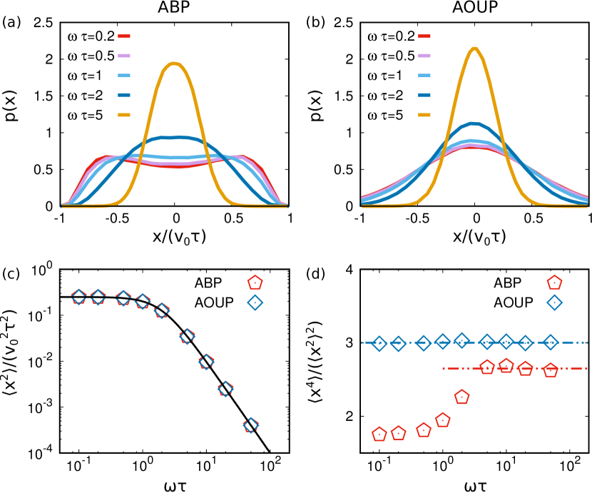
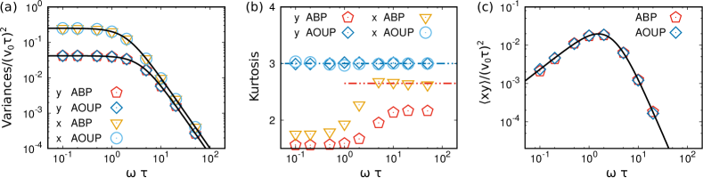
In Fig. 3 the spatial density, , projected onto a single spatial component are plotted for several values of reduced chirality . As expected, the ABP case (Fig. 3 (a)) is richer than the AOUP case (Fig. 3 (b)). The latter is characterized by a Gaussian , whose variance varies with , while the former shows a transition from a bimodal distribution (characterized by two lateral peaks) to a unimodal distribution, when . We consider the moment of this distribution both for ABP and AOUP cases. By symmetry, the first moment is zero, while in both models, the variance of displays a monotonic decrease with starting at . For the variance of the distribution, both AOUP and ABP dynamics show consistent results. Finally, we study the kurtosis of the distribution in the AOUP and ABP to quantify the non-Gaussianity of the latter. In the AOUP case, the kurtosis is equal to being the model Gaussian, whereas in the ABP, the kurtosis is always smaller than as a result of the non-Gaussian nature of the distribution. As increases the kurtosis goes from a value (when is bimodal) to a large asymptotic value sightly smaller than (where is unimodal). This implies that the chirality reduces the non-Gaussianity of the distribution but that the unimodal observed for larger is still non-Gaussian.
IV Chiral active particle in a non-radial potential
In this section, we investigate the dynamics of an active chiral particle in a potential that breaks the rotational symmetry of the system. We consider a harmonic potential with an elliptic shape: . Such a potential introduces an additional dimensionless parameter, , which quantifies the asymmetry of the potential and chose . The remaining dimensionless parameters are and . Here, again we vary the reduced chirality to study the interplay between chirality and asymmetry of the potential.
The asymmetry between the two orthogonal directions in the corresponding equilibrium system would be fully described by the Maxwell-Boltzmann distribution: particles fluctuate around the origin and explore larger regions of space along the direction where the potential gradient is weaker. The generalization to non-chiral active particles is rather straightforward both for AOUP and ABP and does not present significant changes with respect to the symmetric case. Indeed, the non-chiral AOUP in the potential is characterized by a Gaussian distribution similar to the equilibrium case, while the non-chiral ABP, displays accumulation away from the minimum on an ellipsoidal domain rather than a circular one. Intuitively, the accumulation along the more confined direction will be stronger.
IV.1 Spatial distribution and cross-correlations
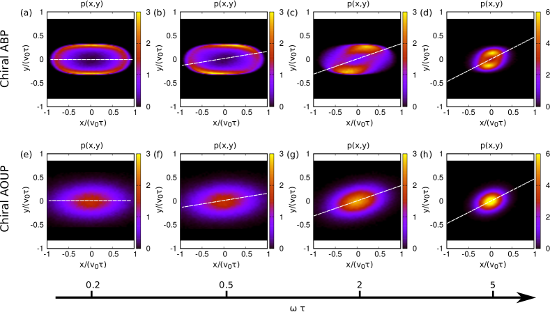
The role of chirality in a harmonic elliptic potential is analyzed by studying the two-dimensional density distribution . The analysis is performed both for ABP and AOUP dynamics and for several values of the reduced chirality (Fig. 4).
In the AOUP case (Fig. 4 (e)-(h)), displays a Gaussian shape, i.e. particles preferentially explore the spatial regions close to the origin, i.e. the minimum of the potential. For small (Fig. 4 (e)), the findings are consistent with the non-chiral scenario: active particles explore the elliptic region around the origin and the chirality slightly decrease the spatial fluctuations as seen in the case of a radial potential. The effect of the chirality emerges for larger values of . As shown in Fig. 4 (f)-(h), the chirality tilts the main axis of the ellipse where the particles accumulate. As a consequence, has a non-Maxwell-Boltzmann shape, since the distribution cannot be expressed as , with . As already remarked, this effect is absent for non-chiral AOUP, and, thus, is purely induced by the interplay between the chirality and the breaking of the radial symmetry of the confining potential. In general, we observe that the increase of increases the tilt angle of the ellipsoid until it reaches a saturation value that by symmetry cannot exceed . Finally, for the chirality leads to a stronger confinement and, thus, decreases the effective temperature of the system without altering the ellipsoidal shape of the potential, as shown from Fig. 4 (g) to Fig. 4 (h). The last observation is consistent with the finding relative to the radial potential of Sec. III.
The numerical results are confirmed by the expression for the probability distribution that reads (see Appendix B)
| (7) |
where the variances and are given by
| (8) | ||||
| (9) |
Expression (7) shows that the interplay between chirality and elliptic confinement induces a cross-correlation . The shape deformation of the probability distribution observed numerically in Fig. 4 is described analytically by the formula:
| (10) |
The cross-correlation vanishes for and displays a non-monotonic behavior as a function of the reduced chirality: it is positive or negative depending on the sign of and on the ratio , and vanishes when the radial symmetry is restored ().
As in the case of radial potential, the ABP dynamics displays a richer scenario (Fig. 4 (a)-(d)). For small reduced chirality (Fig. 4 (a)), particles accumulate away from the potential minimum along the ellipsoid determined by the potential. In particular, particles accumulate more along the direction where the system is more confined, with respect to the direction. In this regime, the increase of the chirality is able to change the orientation of the accumulation area introducing an evident asymmetry in the shape of (Fig. 4 (b)). This effect is enhanced when the reduced chirality is increased, until the regime . Correspondingly, the tendency of particles to climb on the potential is reduced and we can observe larger spatial fluctuations (Fig. 4 (c)). The mechanism that leads to the latter effect is equal to that described in Sec. III. Finally, spatial fluctuations are consistent (Fig. 4 (d)) as if the system was governed by a smaller effective temperature until the accumulation far from the potential minimum is completely suppressed. Again, this is consistent with the results described for a chiral particle in a radial potential.
Both AOUP and ABP dynamics are characterized by a non-Maxwell-Boltzmann distribution with a breaking of the parity symmetry with respect to the (or ) axis that characterizes the elliptic potential. In other words, even if , we have (or equivalently ). This effect emerges in the occurrence of spatial correlations between the Cartesian components of the positions and is purely due to the interplay between chirality and asymmetry of the potential.
IV.2 Moments of the distribution
To quantify this effect we consider the moments of the distribution for and coordinates (Fig. 5). Specifically, Fig. 5 (a) displays the variances and as a function of the reduced chirality . The results are similar for both ABP and AOUP and agree with the theoretical prediction Eq. (8) and Eq. (9). The variances of the distribution that can be interpreted as the effective temperature of the system decrease for both and components approximatively when . However, the effect of chirality manifests itself for smaller values of when the system is less confined, i.e. along the component. For , the chirality decreases the effective temperature of the system as .
Similarly to Fig. 4, to quantify the non-Gaussian nature of the system we study the kurtosis along and components, defined as and . In agreement with our intuition, the kurtosis of the AOUP model for every value of , is equal to . In the ABP case, the two kurtosis display the same qualitative behavior observed in the case of the radial potential in Sec. III. They start from values close to , when the system displays accumulation far from the potential minimum, and then increase with , until reach an asymptotic value slightly smaller than . Here, the non-Gaussian nature of the chiral ABP is more evident along the axis when the system is more confined.
Finally, we plot the cross-correlation , as a function of , where again, the ABP and AOUP display similar results. The cross-correlation of both models is reproduced by the theoretical prediction (10) that shows a non-monotonic behavior. In the regime of small reduced chirality, , the cross-correlation starts from zero and then grows almost linearly until reaches a maximum around . From here, further increase of reduces the value of with a scaling until vanishes.
IV.3 Conditional moments of the distribution
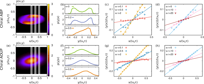
To underpin the breaking of the parity symmetry of the distribution induced by the interplay between chirality and potential asymmetry, we study the conditional distribution of the system, , i.e. the distribution calculated at fixed , defined as (Fig. 6) and the corresponding first conditional moment. Fig. 6 (b) and (f) show for for three positions considered as examples. Panel (b) refers to the ABP dynamics (whose joint distribution, , is reported in Fig. 6 (a)) while panel (c) refers to the AOUP dynamics (whose is reported in Fig. 6 (e)).
In the AOUP case, the distribution has a Gaussian shape in all the cases. However, for , the Gaussian is centered in the origin while by increasing , the center of the Gaussian shifts to values larger than zero. In other words, the parity symmetry (characterizing the elliptic potential) is broken at fixed , i.e. . This is consistent with our analytical prediction
| (11) |
and
| (12) |
is the first conditional moment of the distribution, i.e. the average at fixed , as a function of .
As clear from the shape of and known results in the absence of chirality, the ABP has a non-Gaussian distribution. The conditional distribution of both models shows a similar degree of asymmetry and, in particular, the breaking of the parity symmetry in the distribution . Indeed, at , the displays a fully symmetric bimodal profile. For larger values of , the spatial shape of displays intrinsic asymmetry: the right peak of the distribution becomes larger than the left until the left peak is completely suppressed.
To characterize this asymmetry, we study the first conditional moment of the distribution . This analysis is reported in Fig. 6 (g) and (h) for the AOUP case and in Fig. 6 (c) and (d) for the ABP dynamics for several values of the reduced chirality . In both cases, is described by a linear profile with the same slope, in agreement with our theoretical prediction Eq.(12). shows an almost flat profile for , as expected from the non-chiral case. The slope is an increasing function of the chirality until reaches a maximum for . For larger values of , the slope decreases again until becomes almost flat. This non-monotonicity explains the one observed in the behavior of the cross-correlation (Fig. 5 (c)). Indeed, the non-zero conditional moment induces global cross-correlations in the full distribution and thus, the larger , the larger .
V Conclusions
In summary, we have studied a chiral active particle confined in an external potential, with and without radial symmetry. For radial potentials, the chirality affects the effective temperature of the system both for ABP and AOUP dynamics. Specifically, in the AOUP case, the dynamics displays Gaussian properties due to the linearity of the system with an effective variance that decreases with the chirality. In the ABP case, the chirality reduces the non-Gaussianity of the system, by suppressing the accumulation far from the minimum of the potential typical of the non chiral confined ABP. In other words, the chirality induces a transition from a bimodal to a unimodal density.
For non-radial potentials, the scenario is richer due to the interplay between chirality and asymmetry of the potential which is able to break the parity symmetry in the probability distribution of the system. As a consequence, a non-Maxwell-Boltzmann distribution is found both for chiral ABP and chiral AOUP dynamics. This effect emerges in cross-correlations between the Cartesian components of the position that are present both for chiral ABP and chiral AOUP. The linearity of the AOUP makes possible analytical calculations that allow us to analytically predict the first two moments of the chiral ABP in a harmonic potential.
Acknowledgements.
LC acknowledges support from the Alexander Von Humboldt foundation. HL acknowledges support by the Deutsche Forschungsgemeinschaft (DFG) through the SPP 2265, under grant number LO 418/25-1.Appendix A Derivation effective equation for the probability distribution function
Although the linear models can be solved by considering the Langevin equation for the coordinates and then deriving the distribution function from the first non vanishing cumulants, an equivalent description is possible in terms of an effective Fokker-Planck equation (FPE) for the distribution function. At the linear level, the two methods yield equal results and the choice between them is a matter of taste, but when the potential is non quadratic the FPE method is simpler to implement.
Here, we develop the second method in the case of chiral active particles. For the sake of completeness, we briefly illustrate the basic assumptions leading to a closed equation for the probability density distribution Fox (1986); Hasegawa (2007); Rein and Speck (2016). The equation of motion (1) for can be written for each component as
| (13) |
where the index marks denotes different Cartesian components (for instance, in two dimensions) and is a component of the active force . By standard manipulations, we derive the equation for the associated probability distribution function
| (14) |
where , with the local value assumed by , and . The average is performed over the realizations of the stochastic process and the curly brackets are used to denote a dependence over all the components of a vector.
Since Eq. (14) is not a closed equation for the probability distribution function, we employ the Novikov formula Novikov (1965) to evaluate the average appearing in the last term. This formula is valid for arbitrary Gaussian random functions (Note that the ABP is not described by a Gaussian noise):
| (15) |
where denotes a functional of and on the right hand side is the variational derivative of this functional. The term
| (16) |
is the active force correlation function. Employing Eq. (15) and the definition of , we get
| (17) | |||
The functional derivative of with respect to is given by the following expression valid for for
| (18) |
where the matrix has elements . Combining Eq. (A) with Eq. (18), we find
| (19) | |||
The expressions obtained up to here are exact but not close. Therefore, we employ a closure scheme to obtain a theoretical prediction for the probability distribution. To achieve this goal, we estimate the Eq. (19) as follows:
| (20) |
Here, we have performed three approximations: 1) the factorization of the averages; 2) the replacement of the average of the exponential with the exponential of the average. 3) we have treated as a constant in the time integral in the exponent. Let us remark that the above approximations are exact in the case of quadratic potentials because and not an approximation as in the general case. Going back to Eq. (A), we find
| (21) |
where we have defined the following matrix elements:
| (22) |
Finally, we obtain a closed equation for the probability distribution
| (23) | |||
The method developed here (and in particular the approximations 1), 2) and 3) in Eq. (20)) are exact in the case of a chiral AOUP particle confined in a harmonic potential with radial or non-radial (elliptic) shape. In constrast, for non-linear forces, 1), 2) and 3) are approximations whose accuracy depends on the potential considered. Finally, the method represents only an approximation for the ABP because the Novikov formula, Eq. (15), does not hold. Indeed, the ABP is governed by a non-Gaussian noise because is an orientation with a non-fluctuating unit modulus.
Appendix B Application to simple cases.
The general method presented in the previous appendix is applied to a confining potential (with radial and non-radial symmetry) studied in Sec. III and Sec. IV. First, we estimate the components of the time-autorocorrelation of the active force :
| (26) |
Then, we estimate for a rather general form of central potential, , applying the definition (22) and taking the limit . We obtain the following matrix elements
| (27) | |||
| (28) | |||
| (29) | |||
| (30) |
where we used the abbreviations:
| (31) | |||
| (32) | |||
| (33) | |||
| (34) |
and the primed symbols stand for the first and second derivatives of . After eliminating and in favor of the radial coordinate , the resulting effective Fokker-Planck equation is conveniently written as:
| (35) |
The time independent solution of Eq. (35) is obtained by imposing the vanishing of the radial component, , of the probability current (i.e. minus the expression contained in the square parenthesis in the r.h.s. of Eq. (35)). For the particular case where is harmonic (), expression (35), the difference vanishes and the explicit solution is:
| (36) |
while for arbitrary central potentials the problem can always be reduced to a simple quadrature. Interestingly, it is easy to verify that due to the handedness of the system the tangential component of the probability current does not vanish whenever . In other words, the presence of a radial gradient in the probability density induces a circulation of the particles in the direction orthogonal to it, but such a current does not affect the probability distribution itself. The tangential current reads:
| (37) |
By expressing as a function of the Cartesian components we obtain Eq. (5).
By contrast , in the case of the elliptic quadratic confining potential, , one cannot exploit the radial symmetry of the problem and the equation for the probability density reads:
| (38) | |||
The steady probability can be obtained by first determining its cumulants (Eqs. (8), (9), (10)) from Eq. (B) and using this information to express the pdf as in Eq. (5).
References
- Marchetti et al. (2013) M. C. Marchetti, J. F. Joanny, S. Ramaswamy, T. B. Liverpool, J. Prost, M. Rao and R. A. Simha, Rev. Mod. Phys., 2013, 85, 1143–1189.
- Bechinger et al. (2016) C. Bechinger, R. Di Leonardo, H. Löwen, C. Reichhardt, G. Volpe and G. Volpe, Rev. Mod. Phys., 2016, 88, 045006.
- Löwen (2016) H. Löwen, Eur. Phys. J. Spec. Top., 2016, 225, 2319–2331.
- Liebchen and Levis (2022) B. Liebchen and D. Levis, EPL, 2022, 139, 67001.
- Loose and Mitchison (2014) M. Loose and T. J. Mitchison, Nat. Cell Biol., 2014, 16, 38–46.
- DiLuzio et al. (2005) W. R. DiLuzio, L. Turner, M. Mayer, P. Garstecki, D. B. Weibel, H. C. Berg and G. M. Whitesides, Nature, 2005, 435, 1271–1274.
- Lauga et al. (2006) E. Lauga, W. R. DiLuzio, G. M. Whitesides and H. A. Stone, Biophys. J., 2006, 90, 400–412.
- Riedel et al. (2005) I. H. Riedel, K. Kruse and J. Howard, Science, 2005, 309, 300–303.
- Kümmel et al. (2013) F. Kümmel, B. ten Hagen, R. Wittkowski, I. Buttinoni, R. Eichhorn, G. Volpe, H. Löwen and C. Bechinger, Phys. Rev. Lett., 2013, 110, 198302.
- Zhang et al. (2020) B. Zhang, A. Sokolov and A. Snezhko, Nat. Commun., 2020, 11, 4401.
- Carenza et al. (2019) L. N. Carenza, G. Gonnella, D. Marenduzzo and G. Negro, Proc. Natl. Acad. Sci. U.S.A., 2019, 116, 22065–22070.
- Workamp et al. (2018) M. Workamp, G. Ramirez, K. E. Daniels and J. A. Dijksman, Soft Matter, 2018, 14, 5572–5580.
- Scholz et al. (2021) C. Scholz, A. Ldov, T. Pöschel, M. Engel and H. Löwen, Sci. Adv., 2021, 7, eabf8998.
- Siebers et al. (2023) F. Siebers, A. Jayaram, P. Blümler and T. Speck, Sci. Adv., 2023, 9, eadf5443.
- Wittkowski and Löwen (2012) R. Wittkowski and H. Löwen, Phys. Rev. E, 2012, 85, 021406.
- Van Teeffelen and Löwen (2008) S. Van Teeffelen and H. Löwen, Phys. Rev. E, 2008, 78, 020101.
- Sevilla (2016) F. J. Sevilla, Phys. Rev. E, 2016, 94, 062120.
- Sprenger et al. (2022) A. R. Sprenger, C. Bair and H. Löwen, Phys. Rev. E, 2022, 105, 044610.
- Van Roon et al. (2022) D. M. Van Roon, G. Volpe, M. M. T. da Gama and N. A. Araújo, Soft Matter, 2022, 18, 6899–6906.
- Ao et al. (2015) X. Ao, P. K. Ghosh, Y. Li, G. Schmid, P. Hänggi and F. Marchesoni, EPL, 2015, 109, 10003.
- Caprini and Marconi (2019) L. Caprini and U. M. B. Marconi, Soft Matter, 2019, 15, 2627–2637.
- Fazli and Naji (2021) Z. Fazli and A. Naji, Phys. Rev. E, 2021, 103, 022601.
- Ma and Ni (2022) Z. Ma and R. Ni, J. Chem. Phys., 2022, 156, 021102.
- Semwal et al. (2022) V. Semwal, J. Joshi and S. Mishra, arXiv preprint arXiv:2208.09448, 2022.
- Sesé-Sansa et al. (2022) E. Sesé-Sansa, D. Levis and I. Pagonabarraga, J. Chem. Phys., 2022, 157, 224905.
- Bickmann et al. (2022) J. Bickmann, S. Bröker, J. Jeggle and R. Wittkowski, J. Chem. Phys., 2022, 156, 194904.
- Liao and Klapp (2018) G.-J. Liao and S. H. L. Klapp, Soft Matter, 2018, 14, 7873–7882.
- Liao and Klapp (2021) G.-J. Liao and S. H. Klapp, Soft Matter, 2021, 17, 6833–6847.
- Liebchen et al. (2016) B. Liebchen, M. E. Cates and D. Marenduzzo, Soft Matter, 2016, 12, 7259–7264.
- Liebchen and Levis (2017) B. Liebchen and D. Levis, Phys. Rev. Lett., 2017, 119, 058002.
- Negi et al. (2022) A. Negi, K. Beppu and Y. T. Maeda, arXiv preprint arXiv:2212.14701, 2022.
- Levis and Liebchen (2018) D. Levis and B. Liebchen, J. Phys. Condens. Matter., 2018, 30, 084001.
- Arora et al. (2021) P. Arora, A. Sood and R. Ganapathy, Sci. Adv., 2021, 7, eabd0331.
- Huang et al. (2020) Z.-F. Huang, A. M. Menzel and H. Löwen, Phys. Rev. Lett., 2020, 125, 218002.
- Kruk et al. (2020) N. Kruk, J. A. Carrillo and H. Koeppl, Phys. Rev. E, 2020, 102, 022604.
- Lei et al. (2019) Q.-L. Lei, M. P. Ciamarra and R. Ni, Sci. Adv., 2019, 5, eaau7423.
- Huang et al. (2021) M. Huang, W. Hu, S. Yang, Q.-X. Liu and H. Zhang, Proc. Natl. Acad. Sci. U.S.A., 2021, 118, e2100493118.
- Fruchart et al. (2023) M. Fruchart, C. Scheibner and V. Vitelli, Annu. Rev. Condens. Matter Phys., 2023, 14, 471–510.
- Muzzeddu et al. (2022) P. L. Muzzeddu, H. D. Vuijk, H. Löwen, J.-U. Sommer and A. Sharma, J. Chem. Phys., 2022, 157, 134902.
- Banerjee et al. (2017) D. Banerjee, A. Souslov, A. G. Abanov and V. Vitelli, Nat. Commun., 2017, 8, 1–12.
- Lou et al. (2022) X. Lou, Q. Yang, Y. Ding, P. Liu, K. Chen, X. Zhou, F. Ye, R. Podgornik and M. Yang, Proc. Natl. Acad. Sci. U.S.A., 2022, 119, e2201279119.
- Yang et al. (2021) Q. Yang, H. Zhu, P. Liu, R. Liu, Q. Shi, K. Chen, N. Zheng, F. Ye and M. Yang, Phys. Rev. Lett., 2021, 126, 198001.
- Scheibner et al. (2020) C. Scheibner, A. Souslov, D. Banerjee, P. Surówka, W. T. Irvine and V. Vitelli, Nat. Phys., 2020, 16, 475–480.
- Poggioli and Limmer (2023) A. R. Poggioli and D. T. Limmer, Phys. Rev. Lett., 2023, 130, 158201.
- Debets et al. (2023) V. E. Debets, H. Löwen and L. M. Janssen, Phys. Rev. Lett., 2023, 130, 058201.
- Mijalkov and Volpe (2013) M. Mijalkov and G. Volpe, Soft Matter, 2013, 9, 6376–6381.
- Chen and Ai (2015) Q. Chen and B.-q. Ai, J. Chem. Phys., 2015, 143, 09B612_1.
- Su et al. (2019) J. Su, H. Jiang and Z. Hou, Soft Matter, 2019, 15, 6830–6835.
- Xu et al. (2022) G.-h. Xu, T.-C. Li and B.-q. Ai, Physica A, 2022, 608, 128247.
- Levis et al. (2019) D. Levis, I. Pagonabarraga and B. Liebchen, Phys. Rev. Research, 2019, 1, 023026.
- Samatas and Lintuvuori (2023) S. Samatas and J. Lintuvuori, Phys. Rev. Lett., 2023, 130, 024001.
- Reichhardt and Reichhardt (2013) C. Reichhardt and C. O. Reichhardt, Phys. Rev. E, 2013, 88, 042306.
- Nourhani et al. (2015) A. Nourhani, V. H. Crespi and P. E. Lammert, Phys. Rev. Lett., 2015, 115, 118101.
- Ai et al. (2015) B.-q. Ai, Y.-f. He and W.-r. Zhong, Soft Matter, 2015, 11, 3852–3859.
- Ai et al. (2018) B.-q. Ai, Z.-g. Shao and W.-r. Zhong, Soft Matter, 2018, 14, 4388–4395.
- Reichhardt and Reichhardt (2019) C. Reichhardt and C. J. O. Reichhardt, J. Chem. Phys., 2019, 150, 064905.
- Levis and Liebchen (2019) D. Levis and B. Liebchen, Phys. Rev. E, 2019, 100, 012406.
- Scholz et al. (2018) C. Scholz, M. Engel and T. Pöschel, Nat. Commun., 2018, 9, 1–8.
- Jahanshahi et al. (2017) S. Jahanshahi, H. Löwen and B. ten Hagen, Phys. Rev. E, 2017, 95, 022606.
- Buttinoni et al. (2013) I. Buttinoni, J. Bialké, F. Kümmel, H. Löwen, C. Bechinger and T. Speck, Phys. Rev. Lett., 2013, 110, 238301.
- Solon et al. (2015) A. P. Solon, J. Stenhammar, R. Wittkowski, M. Kardar, Y. Kafri, M. E. Cates and J. Tailleur, Phys. Rev. Lett., 2015, 114, 198301.
- Shaebani et al. (2020) M. R. Shaebani, A. Wysocki, R. G. Winkler, G. Gompper and H. Rieger, Nat. Rev. Phys., 2020, 1–19.
- Caporusso et al. (2020) C. B. Caporusso, P. Digregorio, D. Levis, L. F. Cugliandolo and G. Gonnella, Phys. Rev. Lett., 2020, 125, 178004.
- Caprini and Löwen (2023) L. Caprini and H. Löwen, Phys. Rev. Lett., 2023, 130, 148202.
- Szamel (2014) G. Szamel, Phys. Rev. E, 2014, 90, 012111.
- Martin et al. (2021) D. Martin, J. O’Byrne, M. E. Cates, É. Fodor, C. Nardini, J. Tailleur and F. Van Wijland, Phys. Rev. E, 2021, 103, 032607.
- Maggi et al. (2015) C. Maggi, U. M. B. Marconi, N. Gnan and R. Di Leonardo, Sci. Rep., 2015, 5, 10742.
- Wittmann et al. (2018) R. Wittmann, J. M. Brader, A. Sharma and U. M. B. Marconi, Phys. Rev. E, 2018, 97, 012601.
- Caprini et al. (2019) L. Caprini, U. Marini Bettolo Marconi, A. Puglisi and A. Vulpiani, J. Chem. Phys., 2019, 150, 024902.
- Keta et al. (2022) Y.-E. Keta, R. L. Jack and L. Berthier, Phys. Rev. Lett., 2022, 129, 048002.
- Keta et al. (2023) Y.-E. Keta, R. Mandal, P. Sollich, R. L. Jack and L. Berthier, Soft Matter, 2023, 19, 3871–3883.
- Caprini et al. (2022) L. Caprini, A. R. Sprenger, H. Löwen and R. Wittmann, J. Chem. Phys., 2022, 156, 071102.
- Caprini et al. (2019) L. Caprini, E. Hernández-García, C. López and U. M. B. Marconi, Sci Rep., 2019, 9, 16687.
- Farage et al. (2015) T. F. F. Farage, P. Krinninger and J. M. Brader, Phys. Rev. E, 2015, 91, 042310.
- Buttinoni et al. (2022) I. Buttinoni, L. Caprini, L. Alvarez, F. J. Schwarzendahl and H. Löwen, EPL, 2022, 140, 27001.
- Takatori et al. (2016) S. C. Takatori, R. De Dier, J. Vermant and J. F. Brady, Nat. Commun., 2016, 7, 10694.
- Dauchot and Démery (2019) O. Dauchot and V. Démery, Phys. Rev. Lett., 2019, 122, 068002.
- Caprini et al. (2019) L. Caprini, U. M. B. Marconi and A. Puglisi, Sci. Rep., 2019, 9, 1386.
- Hennes et al. (2014) M. Hennes, K. Wolff and H. Stark, Phys. Rev. Lett., 2014, 112, 238104.
- Rana et al. (2019) S. Rana, M. Samsuzzaman and A. Saha, Soft Matter, 2019, 15, 8865–8878.
- Marini Bettolo Marconi et al. (2017) U. Marini Bettolo Marconi, C. Maggi and M. Paoluzzi, J. Chem. Phys., 2017, 147, 024903.
- Baldovin et al. (2022) M. Baldovin, D. Guéry-Odelin and E. Trizac, arXiv preprint arXiv:2212.06651, 2022.
- Das et al. (2018) S. Das, G. Gompper and R. G. Winkler, New J. Phys., 2018, 20, 015001.
- Woillez et al. (2020) E. Woillez, Y. Kafri and N. S. Gov, Phys. Rev. Lett., 2020, 124, 118002.
- Caprini and Marini Bettolo Marconi (2021) L. Caprini and U. Marini Bettolo Marconi, J. Chem. Phys., 2021, 154, 024902.
- Nguyen et al. (2021) G. H. P. Nguyen, R. Wittmann and H. Löwen, J. Phys. Condens. Matter, 2021, 34, 035101.
- Fodor et al. (2016) É. Fodor, C. Nardini, M. E. Cates, J. Tailleur, P. Visco and F. van Wijland, Phys. Rev. Lett., 2016, 117, 038103.
- Maggi et al. (2017) C. Maggi, M. Paoluzzi, L. Angelani and R. Di Leonardo, Sci. Rep., 2017, 7, 17588.
- Caprini et al. (2022) L. Caprini, U. M. Bettolo Marconi, R. Wittmann and H. Löwen, SciPost Phys., 2022, 13, 065.
- Malakar et al. (2020) K. Malakar, A. Das, A. Kundu, K. V. Kumar and A. Dhar, Phys. Rev. E, 2020, 101, 022610.
- Caraglio and Franosch (2022) M. Caraglio and T. Franosch, Phys. Rev. Lett., 2022, 129, 158001.
- Pototsky and Stark (2012) A. Pototsky and H. Stark, EPL, 2012, 98, 50004.
- Basu et al. (2019) U. Basu, S. N. Majumdar, A. Rosso and G. Schehr, Phys. Rev. E, 2019, 100, 062116.
- Tailleur and Cates (2009) J. Tailleur and M. Cates, EPL, 2009, 86, 60002.
- Solon et al. (2015) A. P. Solon, M. E. Cates and J. Tailleur, Eur. Phys. J. Spec. Top., 2015, 224, 1231–1262.
- Smith et al. (2022) N. R. Smith, P. Le Doussal, S. N. Majumdar and G. Schehr, Phys. Rev. E, 2022, 106, 054133.
- Fox (1986) R. F. Fox, Phys. Rev. A, 1986, 33, 467.
- Hasegawa (2007) H. Hasegawa, Physica A, 2007, 384, 241–258.
- Rein and Speck (2016) M. Rein and T. Speck, Eur. Phys. J. E Soft Matter, 2016, 39, 1–9.
- Novikov (1965) E. A. Novikov, Sov. Phys. JETP, 1965, 20, 1290–1294.