Accelerated, physics-inspired inference of skeletal muscle microstructure from diffusion-weighted MRI

Abstract

Muscle health is a critical component of overall health and quality of life. However, current measures of skeletal muscle health take limited account of microstructural variations within muscle, which play a crucial role in mediating muscle function. To address this, we present a physics-inspired, machine learning-based framework for the non-invasive and in vivo estimation of microstructural organization in skeletal muscle from diffusion-weighted MRI (dMRI). To reduce the computational expense associated with direct numerical simulations of dMRI physics, a polynomial meta-model is developed that accurately represents the input/output relationships of a high-fidelity numerical model. This meta-model is used to develop a Gaussian process (GP) model to provide voxel-wise estimates and confidence intervals of microstructure organization in skeletal muscle. Given noise-free data, the GP model accurately estimates microstructural parameters. In the presence of noise, the diameter, intracellular diffusion coefficient, and membrane permeability are accurately estimated with narrow confidence intervals, while volume fraction and extracellular diffusion coefficient are poorly estimated and exhibit wide confidence intervals. A reduced-acquisition GP model, consisting of one-third the diffusion-encoding measurements, is shown to predict parameters with similar accuracy to the original model. The fiber diameter and volume fraction estimated by the reduced GP model is validated via histology, with both parameters within their associated confidence intervals, demonstrating the capability of the proposed framework as a promising non-invasive tool for assessing skeletal muscle health and function.

1   Introduction

Muscle health is strongly correlated to quality of life [1, 2], motivating a clinical need for interventional methods and quantitative diagnostics that improve muscle health. This need is particularly acute for aging populations, as age-related loss of muscle mass is a primary determinant of decreased muscle function and mobility [3], both of which are linked to increased mortality [4]. Skeletal muscle exhibits a hierarchical structure of elongated, tightly-packed muscle fibers that are surrounded by multiple levels of collagenous extracellular matrix, which plays an important role in force transmission [5]. However, traditional measures of muscle health take limited account for these structural features, restricting our understanding of muscle’s structure–function relationship [6]. Non-invasive measurements of skeletal muscle structure is thus positioned to enable novel insights into the physiological changes of muscle during aging [7] or muscle pathology [8], aiding the development of effective, targeted treatments to increase muscle health.

Currently, biopsy and histology is the most common modality to quantitatively investigate skeletal muscle microstructure, but this measurement approach is invasive, labor-intensive, and highly local to the excised muscle region. A promising alternative with potential to address these limitations is diffusion-weighted magnetic resonance imaging (dMRI), which can provide in-vivo, non-invasive characterization of muscle microstructure organization over the entire muscle volume. dMRI is sensitive to the direction-dependent diffusion distance of water in tissue. In muscle, water diffuses faster in a muscle fiber’s axial direction than transverse direction, where barriers such as cell walls restrict diffusion, resulting in anisotropic diffusion behavior that sensitizes the voxel’s MR signal to these $\sim$$\mu$m length-scale structures. Thus, although the resolution limit of clinical dMRI is $\sim$mm, the underlying tissue microstructure is encoded in the MR signal of each voxel.

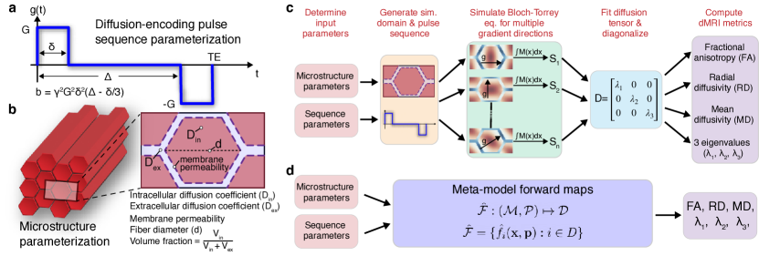
Figure 1: In-silico experiments of skeletal muscle dMRI. (a) Schematic of the generalized diffusion sequence used to represent the diffusion-encoding sequence. (b) Schematic of numerical model of skeletal muscle as periodically packed hexagonal cylinders. (c) Overview of numerical simulation process with the generation of a pulse sequence and microstructural domain, the independent simulation of multiple diffusion directions, construction of diffusion tensors, and finally estimation of dMRI metrics. (d) Overview of meta-model approach where the microstructural and pulse sequence parameters are directly mapped to the dMRI metrics. Here standard DTI metrics are used, but more complex diffusion models can be straightforwardly included.

Decoding the relationship between skeletal muscle microstructure and dMRI measurements is, however, not straightforward. While the forward problem of how microstructure variations influence the dMRI signal has been extensively characterized using numerical models [9, 10, 11, 12], the inverse problem of estimating microstructural parameters from dMRI remains unresolved. Though accurate, numerical models are in general too computationally expensive to use as the basis of solving the inverse problem [13, 14, 15, 16, 17, 10, 18], and, while simplified compartmental models have been used in the past [19, 20, 21, 22, 23], such models do not accurately capture diffusion behavior in skeletal muscle [24]. Another recent model, the Random Permeable Barrier Model, abstracts muscle as a domain of random barriers [25, 26] but does not account for differences in the intracellular and extracellular domain, which is necessary if changes in the extracellular matrix, a critical mediator of skeletal muscle function [5], are to be considered. Thus, there remains a need for models that can accurately characterize the microstructural organization of skeletal muscle.

Here we combine the accuracy and realism of physics-based numerical models with the computational speed of analytical and data-driven models to develop a framework for estimating the microstructural organization of skeletal muscle from dMRI measurements. Beginning with a numerical model of dMRI, we develop a computationally efficient method of inversion while maintaining the accuracy of the numerical solution. We first develop an accelerated solution of the forward problem before using this solution as the basis of a data-driven inverse solution. We conclude with an experimental demonstration of its viability. Overall, this work provides a flexible framework for development of physics-inspired inversion models for the non-invasive estimation of tissue microstructure. While applied here to skeletal muscle modeled using a simplified periodic domain, this methodology is broadly applicable to many classes of biological tissues such as neural and cancer tissues.

2   Fast evaluation of dMRI metrics in muscle

To understand how a voxel’s diffusion MRI (dMRI) signal can be used to estimate the underlying microstructural organization of skeletal muscle, we first consider the forward problem of how microstructural variations influence the dMRI signal and formulate a data-driven, accelerated solution procedure that will aid in the development of an inverse mapping solution.

2.1   Numerical simulation and parameterization

Bloch-Torrey equation

dMRI physics is governed by the Bloch-Torrey equation [27], which describes the time evolution of the dMRI signal in a voxel as

$$\frac{\partial\bm{M}}{\partial t}=-i\gamma\left(\bm{x}\cdot\bm{g}(t)\right)\bm{M}+\nabla\cdot\left(D(\bm{x})\nabla\bm{M}\right)$$ (1)

where $\bm{M}(\bm{x},t)$ is the complex-valued, transverse spin magnetization resulting from exciting longitudinal spins onto the transverse plane and which is manipulated by an externally applied magnetic field ($\bm{x}\cdot\bm{g}(t)$). Here $\gamma$ is the gyromagnetic ratio of hydrogen, $\bm{x}$ is the spin position vector, $\bm{g}(t)$ is the time-varying magnetic field gradient vector used to encode diffusion, and $D(\bm{x})$ is the local diffusion coefficient.

Pulse sequence parameterization

The magnetic field gradient $\bm{g}(t)$ is operator-controlled and can be manipulated to probe different aspects of tissue structure [28]. Here we focus on two related diffusion-encoding pulse sequences: the Stejskal-Tanner pulsed-gradient spin echo (PGSE) [29] and the simulated echo acquisition mode (STEAM) diffusion sequence [30]. If $T_{1}$ and $T_{2}$ effects are set aside, both sequences can be minimally described by the generalized diffusion-weighted sequence described in Fig. 1a that consists of a bipolar magnetic gradient pulse of magnitude $G$ [31, 9]. This generalized sequence is parameterized by four variables, echo time (TE), gradient duration ($\delta$), gradient spacing ($\Delta$), and b-value ($b=\gamma^{2}G^{2}\delta^{2}(\Delta-\delta/3)$). Here, gradient duration is fixed at 5 ms and TE is defined as TE = $\Delta+\delta$, resulting in two free variables of gradient spacing and b-value. The diffusion time of the spins is $t_{d}=\Delta-\delta/3$. However, because our fixed gradient duration of 5 ms is short relative to the gradient spacing timings considered here, for simplicity we approximate the gradient spacing as the diffusion time (i.e. $t_{d}=\Delta$).

Muscle tissue model parameterization

At the microstructural level, skeletal muscle consists of parallel, elongated fibers, each surrounded by a semi-permeable membrane (sarcolemma) and embedded in an extracellular matrix. Informed by histologically based simulations [18], we represent muscle’s microstructural organization via a compact domain of infinitely long, parallel hexagonal cylinders arranged in a periodic array (Fig. 1b). We define a representative elemental volume (REV), which we parameterize to provide a parsimonious description of the muscle microstructure consisting of two morphological parameters (fiber diameter and muscle fiber volume fraction) and three tissue parameters (membrane permeability and intra-/extracellular diffusion coefficients). Water diffusion in the intra- and extracellular domains is characterized by homogeneous (effective) diffusion coefficients that capture the cumulative effects of sub-cellular restrictions within each domain.

Numerical simulations

The Bloch-Torrey equation of Eq. 1 is integrated using the lattice Boltzmann method (LBM) on a D3Q7 stencil, supplemented with appropriate boundary conditions and the initial condition $\bm{M}(\bm{x},t=0)=1$. Intra-domain, semi-permeable boundary conditions handle the effect of spins crossing the muscle’s sarcolemma membrane while modified periodic boundary conditions on the domain boundaries accommodate the non-periodic magnetization accumulation over the periodic REV geometry. Full details of both the boundary conditions and the numerical lattice Boltzmann scheme implementation are available in Naughton et al. [18]

Solving the Bloch-Torrey equation over the prescribed domain results in a spatially localized distribution of the MR signal $\bm{M}(\bm{x},t=\text{TE})$(see Fig. 1c). However, in a physical MR experiment, image formation integrates this local signal distribution to provide the voxel’s dMRI signal. Performing a similar integration to the numerical simulation result

$$S=\left|\left|\int_{V}\bm{M}(\bm{x},t=\text{TE})d\bm{x}\right|\right|$$ (2)

where $V$ is the voxel volume allows matching the numerical simulation result to the MR signal that would be measured on a scanner. This equivalence effectively allows the performance of in silico dMRI experiments, where a known microstructural domain can be defined and a dMRI experiment performed to numerically evaluate the signal such a domain would yield if measured in vivo.

A schematic overview of the simulation pipeline for these in silico experiments is given in Fig. 1c. For each experiment, six non-collinear gradient directions ($S_{i}$) and a non-diffusion-weighted acquisition ($S_{0}$) are simulated and used to fit a diffusion tensor using the fanDTasia ToolBox [32]. In muscle, the diffusion tensor is anisotropic and described by three eigenvalues ($\lambda_{1}$, $\lambda_{2}$, and $\lambda_{3}$), which correspond to the tensor’s principal directions. These eigenvalues are then used to compute the tensor invariants of fractional anisotropy $\text{FA}=\sqrt{\frac{(\lambda_{1}-\lambda_{2})^{2}+(\lambda_{2}-\lambda_{3})^{2}+(\lambda_{3}-\lambda_{1})^{2}}{2(\lambda_{1}^{2}+\lambda_{2}^{2}+\lambda_{3}^{2})}}$, mean diffusivity MD = $(\lambda_{1}+\lambda_{2}+\lambda_{3})/3$, and radial diffusivity RD = $(\lambda_{2}+\lambda_{3})/2$, which characterize the diffusion anisotropy and magnitude within the voxel. While here a standard diffusion tensor imaging (DTI) model is used, more complex post-processing and diffusion models can straightforwardly be incorporated.

2.2   Model acceleration via meta-modeling

While accurate, numerical simulation of the forward problem is computationally expensive, with a typical in silico dMRI experiment taking 1-2 minutes per voxel. Coupled with direct inverse solution approaches, which require many iterative forward solutions, use of this numerical model results in solution times on the order of 45 minutes per voxel to estimate underlying microstructural parameters [33]. Scaled to a typical 64$\times$64 (or larger) resolution dMRI image with multiple slices, this approach quickly becomes computationally infeasible.

To accelerate solution times, we exploit the insight that the spatial distribution of the signal within the microstructural domain—which is computationally expensive to obtain—is not directly needed and can be bypassed by the deployment of a data-driven forward mapping

$$\mathcal{F}:(\mathcal{M},\mathcal{P})\mapsto\mathcal{D}$$ (3)

that directly maps the microstructural ($\mathcal{M}\in\mathbb{R}^{m}$) and diffusion-encoding sequence ($\mathcal{P}\in\mathbb{R}^{p}$) domains to the dMRI metrics ($\mathcal{D}\in\mathbb{R}^{d}$).

Polynomial meta-model

We approximate the forward mapping $\mathcal{F}$ using a set of meta-models to generate individual mappings for each dMRI metric

$$\hat{\mathcal{F}}=\{\hat{f}_{i}(\mathbf{x},\mathbf{p}):i\in D\}$$ (4)

for $D\in\{$FA, MD, RD, $\lambda_{1}$, $\lambda_{2}$, $\lambda_{3}$$\}$. These meta-models (Fig. 1d) approximate the relationship between the inputs ($m=5$ microstructural parameters $\mathbf{x}\in\mathcal{M}$ and $p=2$ sequence parameters $\mathbf{p}\in\mathcal{P}$) and outputs ($d=6$ dMRI metrics) of the numerical model pipeline in a data-driven manner with no regard for the underlying physics.

While a number of meta-modeling frameworks [34] and machine learning techniques [35, 36] are available, here we adopt the polynomial chaos expansion approach, which models the evolution of a system with stochastic inputs [37, 38]. Each meta-model is represented as an expansion of a properly selected polynomial basis truncated to a finite basis set

$$\hat{f}_{i}(\mathbf{x},\mathbf{p})=\sum_{j=0}^{T}\alpha_{j}\ \bm{\psi}_{j}(\mathbf{z})$$ (5)

where $\alpha_{j}$ are the basis weights, $\bm{\psi}_{j}$ are multivariate polynomials, $T+1=(N+C)!/(N!~{}C!)$ is the number of terms in the basis set for a maximum polynomial order of $C$ and $N=m+p$ input parameters, and $\mathbf{z}=\Gamma(\mathbf{x},\mathbf{p})\in[-1,1]^{N}$ is the normalized transformation of the uniformly distributed microstructural parameter ranges given in Table 1 to the interval $[-1,~{}1]$. The choice of basis polynomials $\bm{\psi}_{j}$ is determined by the parameter distribution, which, for the uniform distribution considered here, is the set of Legendre polynomials [39].

Table 1: Microstructure and pulse sequence parameter ranges spanned by meta-model.

Parameter	Range
Muscle fiber diameter	10	–	80	$\mu$m
Volume fraction	0.7	–	0.95
Membrane permeability	10	–	100	$\mu$m/s
Intracellular diffusion	0.5	–	2.5	$\mu$m2/ms
Extracellular diffusion	0.5	–	2.5	$\mu$m2/ms
Diffusion time	10	–	750	ms
b-value	300	–	1200	s/mm2

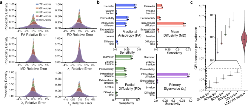
Figure 2: Meta-model acceleration of dMRI simulations. (a) Density plots of meta-model error for dMRI metrics of FA, MD, RD, $\lambda_{1}$, $\lambda_{2}$, and $\lambda_{3}$. As the order of the polynomial basis set increases, the meta-model accuracy improves. (b) Global sensitivity indices of the 7${}^{\text{th}}$-order meta-model (solid color) and LBM numerical model (white) demonstrating the meta-model captures the global behavior of parameter variation. Results for $\lambda_{2}$ and $\lambda_{3}$ and not shown as they are nearly identical to RD results. (c) The computational cost of meta-model evaluation increases with polynomial order but remains lower than the numerical model in all cases. The 7${}^{\text{th}}$-order meta-model has a mean evaluation time 3 orders of magnitude (1000x) faster than the numerical model and a maximum evaluation time 5 orders of magnitude faster.

Meta-model generation

To generate the meta-model, a previously reported data set of 80,000 parameter sets [9] was used to fit the weights $\alpha_{j}$ of the PC expansion using a 70/30 train/test split. Data was fit using least-squares linear regression by the open-source ChaosPy Python package [40] . The dataset was generated via a Sobol sampling method, which is a low discrepancy sampling method, meaning the input data used to construct the model are evenly distributed across the input space [41]. Each dataset entry consists of a microstructural parameter set $\mathbf{x}$, a pulse sequence parameter set $\mathbf{p}$, and dMRI metrics $f_{i}(\mathbf{x},\mathbf{p})$ for $i\in D$ that resulted from an in silico dMRI experiment following the procedure described in Section 2.1. Maximum polynomial orders $C\in\{3,...7\}$ of the Legendre polynomial basis were considered.

Accuracy and sensitivity

Evaluating the trained meta-models over the test data resulted in a vector of meta-model estimates $\mathbf{\hat{f}}_{i}$ and an associated vector of ground-truth, numerically-simulated dMRI metrics $\mathbf{f}_{i}$. To quantify the accuracy of the meta-model we consider the accuracy of each dMRI metric independently and define a relative error metric

$$\text{e}_{i}=\frac{\hat{f}_{i}(\mathbf{x},\mathbf{p})-f_{i}(\mathbf{x},\mathbf{p})}{\max(\textbf{f}_{i})-\bar{\textbf{f}_{i}}}$$ (6)

where $\bar{\textbf{f}_{i}}$ is the mean of the vector $\textbf{f}_{i}$.

Figure 2a shows the distribution of relative error between the meta-models and the ground-truth numerical simulations in the test split of the data set for each dMRI metric. For increasing polynomial order, the accuracy of the meta-model improves, with errors on the order of $<$1% for the meta-model constructed from 7${}^{\text{th}}$-order polynomials, showing it to be an accurate representation of the underlying numerical model. The test data used to quantify accuracy is extracted from the same Sobol sequence as the training data, implying these results are an upper limit of the meta-model error as the test data is sampled at points far away from the training data. To further quantify the performance of the meta-model, the sensitivity of the meta-model to changes in its inputs was computed and compared to the sensitivity of the underlying numerical model reported in [9]. The results, shown in Fig. 2b, show the sensitivity indices are nearly identical to those of the full numerical model, demonstrating that the fitted meta-model accurately captures the global responses of the underlying numerical model for each microstructural input parameter.

Computational efficiency

As the polynomial order increases, the accuracy of the meta-model increases, but so too does the computational evaluation time (Fig. 2c). However, the trained meta-models are drastically faster to evaluate than the underlying LBM numerical model for all polynomial orders, with the mean evaluation time of the 7${}^{\text{th}}$-order meta-model three orders of magnitude faster than the mean evaluation time of the numerical model. This speed-up becomes even more pronounced when maximum evaluation time is considered, with the 7${}^{\text{th}}$-order meta-model five orders of magnitude faster than the numerical model. The time-stepping nature of the LBM numerical model leads to its evaluation time being directly proportional to the diffusion time of the simulated sequence. The analytical nature of the meta-model, in contrast, obviates this limitation, leading to more uniform evaluation times.

3   Inverse problem solution

We next turn to the inverse problem of estimating microstructural organization from dMRI data. Previous attempts have generally consisted of iteratively solving a forward model to converge on a set of microstructural parameters [33, 19, 20, 21, 22, 23, 25]; however, such approaches are computationally expensive due to the large number of function evaluations required. Our goal here is to instead define a data-driven inverse map

$$\mathcal{G}:\mathcal{S}\mapsto\mathcal{M}$$ (7)

that directly maps the dMRI measurement domain $\mathcal{S}\in\mathbb{R}^{s\times d}$ to the microstructure parameter domain $\mathcal{M}\in\mathbb{R}^{m}$. While machine learning regression approaches have been widely used to generate cost-effective inverse solutions for a range of problems [35, 42, 43], many traditional approaches, such as random forest regression or deep neural networks, do not provide uncertainty measures for their outputs, which can be critically important to interpreting results. To address this, here we utilize Gaussian process (GP) regression, or kriging, to generate a data-driven inverse map that additionally provides confidence intervals of its predictions, substantially increasing the interpretability, and thus utility, of the estimates [44].

3.1   Gaussian process regression

Each microstructural parameter is modeled as its own Gaussian process, leading to the inverse map

$$G=\{g_{i}(\mathbf{s}):i\in M\}$$ (8)

where $\mathbf{s}\in S$ is a vector of dMRI metrics acquired by a set of $s$ diffusion-encoding sequences (defined below) and $M$ is the domain of all five microstructural parameters.

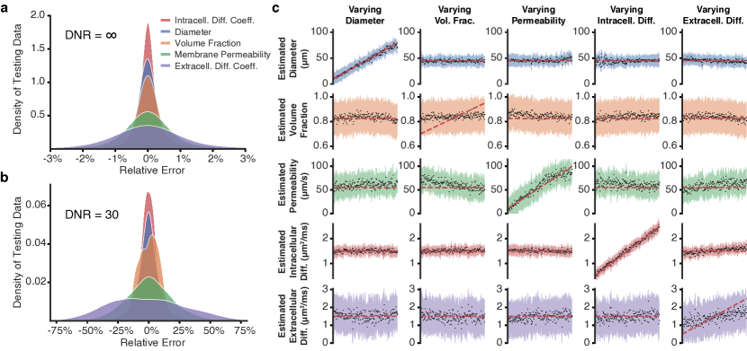
Figure 3: Gaussian process inverse mapping. (a) Error density of GP model when evaluating synthetic, noise-free dMRI measurements. (b) Error density of GP model when evaluating noisy dMRI measurements with a diffusion-to-noise ratio of 30. (c) GP model results for dMRI measurements (DNR=30) when a single microstructural parameter is varied at a time. For each column, 200 meta-model evaluations were made as the varied microstructure parameter was linearly increased. Results are organized column-wise with vertical alignment relating to the same dMRI measurement and the dashed line denoting the true microstructural value.

A Gaussian process is a generalization of a Gaussian probability distribution. It is a collection of random variables, any finite subset of which has a joint Gaussian distribution [45]. A Gaussian process

$$g_{i}(\mathbf{s})\sim\mathcal{GP}\left(m_{i}(\mathbf{s}),k_{i}(\mathbf{s},\mathbf{s}^{\prime})\right){.}$$ (9)

is defined by a mean function $m_{i}(\mathbf{s})$ and covariance function $k_{i}(\mathbf{s},\mathbf{s}^{\prime})$ over the inputs $\mathbf{s}$. In practice, is it common to either subtract out the mean or directly set $m_{i}(\mathbf{s})=0$, allowing the Gaussian process to be written as

$$g_{i}(\mathbf{s})\sim\mathcal{N}\left(0,k_{i}(\mathbf{s},\mathbf{s}^{\prime})\right)$$ (10)

where $\mathcal{N}(\cdot)$ denotes a normal distribution.

A key component of Gaussian process regression is the selection of the covariance kernel function $k_{i}(\mathbf{s},\mathbf{s}^{\prime})$, which can strongly influence the model’s accuracy. Progress has been made towards automated kernel selection [46]; however empirical kernel selection is still generally required. Here, a radial basis function kernel and a linear kernel are combined with a Gaussian noise kernel to form the covariance function

$$\begin{split}k_{i}(\mathbf{s},\mathbf{s}^{\prime})=&\sigma^{2}_{r}\exp\left(-\frac{1}{2l^{2}}(\mathbf{s}-\mathbf{s}^{\prime})^{2}\right)+\\ &\sigma^{2}_{l}(\mathbf{s}-c)(\mathbf{s}^{\prime}-c)+\sigma^{2}_{n}\delta_{ij}\end{split}$$ (11)

where kernel variances $\sigma$ and length-scales $l$, $c$ are hyperparameters tuned to maximize the log marginal likelihood of the model over the training data, which consists of the set of microstructural parameters $\mathbf{g}_{i}$ and associated dMRI measurements $S=\{\mathbf{s}_{1},\mathbf{s}_{2},...,\mathbf{s}_{n}\}$. A unique set of hyperparameters is tuned for each GP $g_{i}(\mathbf{s})$. While it is possible to incorporate information about relationships between microstructural parameters (coregionalization), such methods substantially increase the difficulty of hyperparameter optimization and often lead to over-fitting [45]. As such, they were not considered here.

With the kernel defined, the inverse problem can be formulated as: given a set of $n$ training observations of microstructural parameters $\mathbf{g}_{i}$ and their set of corresponding dMRI measurements $S$, predict the microstructural parameter distribution $\mathbf{g}_{i}^{*}\sim\mathcal{N}(0,K_{i}(S^{*},S^{*}))$ given the set of $n^{*}$ dMRI measurements $S^{*}$. According to the definition of Gaussian processes, the joint probability distribution of these training and evaluation outputs is also Gaussian and can be written

$$\begin{bmatrix}\mathbf{g}_{i}\\ \mathbf{g}_{i}^{*}\end{bmatrix}\sim\mathcal{N}\left(0,\begin{bmatrix}K_{i}(S,S)&K_{i}(S,S^{*})\\ K_{i}(S^{*},S)&K_{i}(S^{*},S^{*})\end{bmatrix}\right)$$ (12)

where, $K_{i}(S^{*},S)$ is the $n^{*}\times n$ matrix of the covariances of $S^{*}$ and $S$ based on Eq. 11 (and similarly for all $K_{i}(\cdot,\cdot)$).

To include the training data information in our estimation of $\mathbf{g}_{i}^{*}$, we condition the joint Gaussian prior distribution of Eq. 12 on the observations $\mathbf{g}_{i}$, resulting in the posterior distribution

$$\mathbf{g}_{i}^{*}|S^{*},S,\mathbf{g}_{i}\sim\mathcal{N}\left(\bar{\mathbf{g}}_{i}^{*},\mathrm{cov}(\mathbf{g}_{i}^{*})\right)$$ (13)

where the mean $\bar{\mathbf{g}}_{i}^{*}$ and covariance matrix $\mathrm{cov}(\mathbf{g}_{i}^{*})$ are

$$\bar{\mathbf{g}}_{i}^{*}=K_{i}(S^{*},S)K_{i}(S,S)^{-1}\mathbf{g}_{i}$$ (14)

$$\mathrm{cov}(\mathbf{g}_{i}^{*})=K_{i}(S^{*},S^{*})-K_{i}(S^{*},S)K_{i}(S,S)^{-1}K_{i}(S,S^{*})$$ (15)

Note that both the mean $\bar{\mathbf{g}}_{i}^{*}$ and covariance matrix $\mathrm{cov}(\mathbf{g}_{i}^{*})$ are solely functions of the training observations $\mathbf{g}_{i}$, the training dMRI data $S$, and the observed dMRI data $S^{*}$, all of which are known. Thus, given a set of dMRI measurements $\mathbf{s}$ , for each microstructural parameter we can evaluate the predicted posterior distribution to compute a mean microstructural estimate $\mu_{i}(\mathbf{s})$ (Eq. 14) and its variance $\sigma_{i}(\mathbf{s})$ (Eq. 15), which is then scaled to determine a 95% confidence interval.

3.2   dMRI-inversion model formulation

To formulate an inverse mapping, a fixed set of diffusion-encoding parameter sets must first be defined. Because multiple microstructural parameters are being estimated, multiple diffusion-encoding measurements are required to constrain the inverse problem. Here, we focus on the effect of diffusion time and b-value. Multiple b-values allows sensitivity to non-Gaussianity of the diffusion behavior [47] while varying diffusion time sensitizes the diffusion behavior to microstructural features at different length scales [25, 48, 49].

Five b-values (400, 600, 800, 1000, and 1200 s/mm²) and six diffusion times (20, 50, 100, 200, 400, 700 ms) were selected to generate $s=30$ unique diffusion-encoding parameter sets. All sequences are here modeled as STEAM sequences represented by the generalized diffusion sequence with described in Section 2.1. The b-value is achieved by adjusting the diffusion-encoding gradient strength. Both b-values and diffusion times were selected to span the ranges viable for a clinical scanner using a STEAM sequence for skeletal muscle dMRI.

Model training

To generate training data for the GP model, the 7${}^{\text{th}}$-order meta-model was sampled using a Sobol sequence at 9000 microstructural parameter combinations. The meta-model was evaluated for FA, $\lambda_{1}$, and RD for all thirty diffusion-encoding parameter sets, resulting in 90 input measurements ($\lambda_{2}$ and $\lambda_{3}$ were not considered due to their strong similarity to RD). To reduce the dimensionality of the input data, these 90 inputs were combined into a single vector for each parameter set, and principal component analysis (PCA) was performed on the vectors. The 20 dimensions that best described the observed input variance were selected, scaled to zero-mean and unit-variance, and used as the inputs to the GP model.

The meta-model produces noise-free estimates of dMRI metrics; however, accounting for the influence of noise in dMRI measurements is a critical consideration of any inverse solution [50] and so synthetic noise was injected into the training data. Because the meta-model directly outputs dMRI metrics, it is not possible to incorporate noise directly into the raw signal. Instead, Gaussian noise is injected into the dMRI metrics based on a diffusion-to-noise (DNR) ratio. Five copies of the dMRI metrics were created. One remained noise-free with noise added to the others to achieve a DNR of 30.

The open-source GPy Python package was used to fit the GP model and optimize the GP kernel hyperparameters using the L-BFGS-B algorithm [51]. For large data sets such as those considered here, this optimization can be slow. To accelerate the process, subsets of increasing size containing only noise-free data were iteratively used to optimize the hyperparameters over smaller data sets, allowing the GP model to quickly learn the coarse structure of the underlying data.

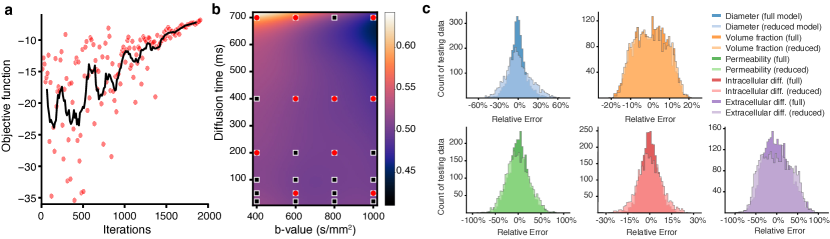
Figure 4: Optimized diffusion-encoding sequence selection. (a) Convergence of CMA-ES algorithm’s maximization of the objective function over 2000 iterations to select a compact set of ten diffusion-encoding sequences. (b) Map of the variance between the 1024 different microstructural parameters used for different diffusion time and b-value combinations. The locations of the sequence used for the full GP model (black boxes; b=1200 s/mm2 not visualized) and ten sequences selected by the CMA-ES algorithm (red circles) are overlaid. (c) Comparisons of the relative error histograms of the full and reduced sequence GP models for all microstructural parameters shows limited loss in accuracy when the reduced set of sequences are used.

GP model accuracy

The 7${}^{\text{th}}$-order meta-model was sampled using a new Sobol sequence to generate 3000 data-points. Evaluating the test data resulted in vectors of mean microstructural estimates $\bm{\mu}_{i}$ for $i\in M$ and associated vectors of ground-truth microstructural values $\mathbf{x}_{i}$. To quantify GP model accuracy, we define the relative error metric

$$\text{e}=\frac{\mu_{i}(\mathbf{s})-x_{i}(\mathbf{s})}{\bar{\mathbf{x}}_{i}}$$ (16)

where $x_{i}(\mathbf{s})$ is the true microstructural parameter. The accuracy of the model was quantified against both noise-free (Fig. 3a) and noisy (DNR = 30; Fig. 3b) versions of the test data. While the accuracy of microstructural estimates decreases in the presence of noise, the GP model’s high accuracy when given noise-free data demonstrates both the general invertability of the problem and that the GP model is learning the underlying data structure.

A third test is depicted in Fig. 3c wherein the test data is generated by evaluating the forward meta-model and varying only a single microstructural parameter at a time (diagonal entries) while holding all others constant. As Fig. 3c shows, the GP model is able to accurately capture changes in fiber diameter, membrane permeability, and intracellular diffusion coefficient while struggling to identify variations in the volume fraction or extracellular diffusion coefficient. However, the GP model’s confidence intervals in its mean estimate of the volume fraction and extracellular diffusion coefficient are wide, indicating the mean parameter estimate should be interpreted with caution. In contrast, its accurate estimates of fiber diameter, membrane permeability, and intracellular diffusion coefficient are accompanied by comparably narrower confidence intervals, indicated confidence in the mean estimate.

3.3   Reduced diffusion-encoding model

While it is broadly known how different diffusion-encoding pulse profiles affect the MR signal [47], which combinations of sequences encode the most microstructural information about the tissue is less clear. In the prior section, this uncertainty is addressed by densely sampling the possible combinations of diffusion time and b-value (Fig. 4b). However, because imaging time is proportional to the total number of diffusion-encoding parameter sets utilized, reducing the number of parameter sets used is paramount for clinical translatablility.

To identify a compact set of diffusion-encoding sequences, the 5${}^{\text{th}}$-order meta-model (for computational efficiency) was sampled at four uniformly spaced points for all five microstructural parameters ($N=1024$) and FA, MD, RD, and $\lambda_{1}$ metrics were precomputed for 80 pulse sequences defined on a grid of four evenly-spaced b-values between 400 and 1000 s/mm² and twenty evenly-spaced diffusion times between 10 and 700 ms. For a candidate subset of $s=10$ sequences, a 3${}^{\text{rd}}$-order polynomial surface was fit to the dMRI metrics at each of the $N$ microstructural parameter sets. The fitted surface was evaluated at all 80 pulse sequences resulting in a vector $\mathbf{q}_{i_{n}}$ for $i\in\{\text{FA, MD, RD, $\lambda_{1}$}\}$ that was compared to the precomputed meta-model dMRI metrics $\mathbf{Q}_{i_{n}}$. An objective function was defined to quantify the ability of a subset of ten diffusion-encoding pulse sequences to capture the structural information encoded by this full set of sequences according to

$$\phi=-\sum_{n=1}^{N}\Big{|}\Big{|}\big{(}||\mathbf{q}_{i_{n}}-\mathbf{Q}_{i_{n}}||:i\in\{\text{FA, MD, RD, $\lambda_{1}$}\}\big{)}\Big{|}\Big{|}$$ (17)

We maximized Eq. 17 using the CMA-ES algorithim (Fig. 4a), which is a non-linear, derivative-free evolutionary search algorithm [52]. The ten sequences selected by the CMA-ES algorithm were matched to the nearest corresponding pulse sequences used to define the previous GP model (Fig. 4b)

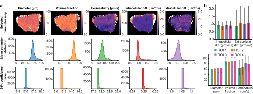
Figure 5: Experimental estimates of microstructure organization. (a) Voxel-wise estimates of all five microstructural parameters for a single slice of the bovine biceps femoris dMRI data (top row); histograms of the distribution of the five microstructural parameters over the entire 3D domain after thresholding to exclude outliers related to edge voxels (middle row); and distribution of 95% confidence intervals from GRP model over entire 3D domain (bottom row). (b) Averaged estimates and 95% confidence intervals for all five microstructural parameters of four ROIs within the tissue.

Reduced GP model

A second GP model was fit using this reduced set sequences following the same process as before. A comparison of the full and reduced GP model’s accuracy is shown in Fig. 4c, where, to test the model’s generalization performance, both models are tested against a dataset of 3000 solutions generated by the LBM numerical model. Results for both models are broadly similar, with only a slight decrease in accuracy for the reduced pulse sequence model. Using only one-third the diffusion-encoding measurements, this set of $s=10$ sequences defines a more experimentally plausible set of sequences for use in a physical experiment.

4   Experiments

4.1   Voxel-wise microstructure estimation

To test the accuracy of the proposed inversion scheme, a validation experiment was performed. Tissue from a bovine biceps femoris was procured and a 7 cm sample from a unipenate portion was excised and imaged on a Siemens Prisma 3T scanner using a prototype diffusion-weighted STEAM sequence with EPI readout [30]. Ten diffusion-weighted measurements based on the sequences selected by the CMA-ES algorithm were obtained, each with twelve gradient directions and 2 averages. Twenty slices with a $64\times 64$ FOV matrix and 3.4 mm isotropic voxels were acquired. For all scans, TE = 49 ms. For scans with $\Delta>500$ ms, TR = 1500 ms, otherwise TR = 1200 ms. The experiment took approximately one hour to complete. Image data was thresholded and post-processed with FSL [53] to compute diffusion metrics for each voxel. This dataset (9607 voxels) was read into the reduced GP model and used to produce voxel-wise estimates of the microstructural parameters. Here, $\lambda_{3}$ was used instead of RD to better capture microstructural data based on the hypothesis that $\lambda_{3}$ is a stronger reflection of fiber-level transverse diffusion behavior [54, 55]. Additionally, four ROIs were manually defined within the 3D tissue volume, consisting of between 12 and 32 voxels. Diffusion metrics from these voxels were averaged and used to estimate mean microstructural parameters and confidence intervals for the ROI.

Figure 5a (top row) shows the resulting voxel-wise estimates of all five microstructural parameters for a representative slice of the 3D volume. For each microstructural parameter, estimation for all 9607 voxels took $39.18\pm 0.05$ seconds (4 ms/voxel). Parameter ranges appear consistent throughout the muscle beyond slight variation in voxels near the edge of the tissue, where partial volume effects likely distorted the signal. Figure 5b (middle row) shows histograms of the distribution of the five microstructural parameters after thresholding to exclude outliers related to edge voxels while Fig. 5c (bottom row) shows the distribution of the associated 95% confidence intervals. Mean parameter estimates have unimodal distributions with relatively small tails while the confidence intervals exhibit a sharp minimum bound, indicative of experimental noise limiting the confidence of the inversion scheme. Results from the four ROIs are shown in Fig. 5d.

4.2   Histological validation

Validation of microstructure estimates is challenging due to the difficulty of independently measuring many of the estimated microstructural parameters, in particular intracellular and extracellular diffusion coefficients or sarcolemma membrane permeability. Morphological parameters, such as fiber diameter and volume fraction, are comparably easier to verify through histological examination. Tissue from two ROIs (1 and 2) was excised and fixed in 10% buffered formalin for one week. After fixation, tissue was dehydrated, embedded in paraffin wax, sectioned, and stained with hematoxylin and eosin. Microscopy images were acquired at 40x magnification. Images were processed using ImageJ [56] to binarize data, and fiber diameters for each ROI were approximated by the median Feret diameter using the ‘Analyze Particles’ tool in ImageJ. During tissue processing, distortion due to tissue shrinkage can skew measurements, possibly leading to underestimation of fiber diameter. To mitigate this bias and establish an upper bound of fiber diameters, binarized images were processed in Matlab with a watershed transform to skeletonize the domain and eroded using ImageJ to reestablish a uniformly thin extracellular space. This processing effectively swells the fibers to fill the domain and the Feret diameter was again measured. Muscle fiber volume fractions were also computed for both the original and swelled domains.

Table 2: Diameter and volume fraction measurements from histological examination of ROIs 1 and 2 for the original and swelled domains as well as the GP model estimates with 95% confidence interval (CI).

	Fiber diameter			Volume fraction
	Original	Swelled	GP estimate $\pm$ 95% CI	Original	Swelled	GP estimate $\pm$ 95% CI
ROI 1	55.2 $\mu$m	73.9 $\mu$m	62.3 $\pm$ 17.0 $\mu$m	0.674	0.894	0.894 $\pm$ 0.134
ROI 2	51.0 $\mu$m	62.0 $\mu$m	62.9 $\pm$ 17.0 $\mu$m	0.514	0.902	0.883 $\pm$ 0.134

The histologically-measured fiber diameters and volume fractions of the ROIs are reported in Table 2 along with the estimated mean and confidence intervals of the GP model. The measured fiber diameters fall within the predicted range, though there is a relatively wide confidence interval. The confidence intervals of the ROIs are lower than the voxel-wise results due to the averaging of the dMRI metrics over the ROI increasing the SNR of the data. These results demonstrate that the GP model can provide estimates of the fiber diameter that agree with histological measurements. The swelled measurements of volume fraction also match the GP estimates while the results from the original histology measurements are lower than the estimated range. The large confidence range of the volume fraction cautions against giving too much credence to this parameter estimate and shrinkage and other deformation of the tissue during fixation and processing make it difficult to know which volume fraction estimate is the most valid.

5   Discussion

This paper presents a framework for computationally efficient estimation of skeletal muscle microstructural parameters from dMRI. Use of Gaussian processes (GP) in the inverse mapping provides not only voxel-wise microstructure estimates but also uncertainty intervals, which increases the utility and interpretability of the model’s estimates by identifying when a microstructure estimate can be strongly relied on or when it is likely an arbitrary guess. There are two approaches to interpreting these confidence intervals. The first is adopted here, where a single mean value represents the microstructure of the entire voxel and the confidence intervals are then a measure of uncertainty. The second interpretation treats the predicted Gaussian distribution as representing a distribution of parameters within the voxel (e.g. distribution of fiber diameters). Considering the distribution of microstructures that occur in skeletal muscle, such a perspective may further extend the insights available from GP-based inverse models.

In the presence of noise, the parameters the GP inversion scheme accurately estimates in Fig. 3 (diameter, intracellular diffusion coefficient, and membrane permeability) are notably the parameters with the highest sensitivity indices of the forward models reported in Fig. 2b. Given noise-free data, the inverse map model accurately inverts the problem for all five microstructural parameters, indicating the GP model learns the underlying data structure and suggesting model accuracy can be increased if higher SNR measurements are acquired.

The framework developed here has a flexible, modular structure. It consists of multiple independent components, each of which can be refined or exchanged with alternative approaches to improve future iterations. For example, incorporating more sophisticated parameterizations of muscle microstructure will further improve the realism of the forward problem, while use of alternative meta-modeling techniques, such as deep neural networks may increase the accuracy and computational efficiency of its meta-model approximation. The diffusion-encoding schemes considered here can also be advanced by increasing the fidelity of the PGSE and STEAM sequence simulations or by considering additional diffusion-encoding sequences such as OGSE [57]. Finally, combining diffusion-encoding sequence optimization with compressed sensing frameworks may allow further reduction in the diffusion-encoding sequences needed, aiding in clinical feasibility and translatability efforts by further reducing imaging time.

6   Conclusion

Overall, this work provides a flexible, modular framework for development of physics-inspired, data-driven inversion models for the estimation of tissue microstructure from dMRI. To reduce the computational expense associated with direct numerical simulations of dMRI physics, a polynomial meta-model is developed that accurately represents the numerical model and is used to develop a Gaussian process regression model to provide voxel-wise microstructural estimates and confidence intervals. The proposed methodology is broadly applicable to additional classes of biological tissues such as neural and cancer tissues, extending its potential impact. Applied here to skeletal muscle, its experimental implementation and validation demonstrates the capability of the framework as a promising non-invasive tool for in vivo assessment of skeletal muscle health and function.

Data Availability

Code and model weights for the meta-model and Gaussian process regression models presented in this paper are available upon request from the authors.

Acknowledgements

This work was supported in part by an NSF GRFP (N.N.), the R.A. Pritzker endowed chair (J.G.), NSF grants CMMI-1437113, and CMI-1762774 (J.G.), and NIH grants HL090455 and EB018107 (J.G.).

References

- [1] Robert T Kell, Gordon Bell and Art Quinney “Musculoskeletal fitness, health outcomes and quality of life” In Sports Medicine 31.12 Springer, 2001, pp. 863–873
- [2] Dinesh Samuel, Philip Rowe, Victoria Hood and Alexander Nicol “The relationships between muscle strength, biomechanical functional moments and health-related quality of life in non-elite older adults” In Age and Ageing 41.2 Oxford University Press, 2011, pp. 224–230
- [3] Ronenn Roubenoff “Origins and clinical relevance of sarcopenia” In Canadian Journal of Applied Physiology 26.1, 2001, pp. 78–89
- [4] Dennis T. Villareal et al. “Physical frailty and body composition in obese elderly men and women” In Obesity Research 12.6 Wiley-Blackwell, 2004, pp. 913–920
- [5] Peter P Purslow “The structure and functional significance of variations in the connective tissue within muscle” In Comparative Biochemistry and Physiology Part A: Molecular & Integrative Physiology 133.4 Elsevier, 2002, pp. 947–966
- [6] Rosaly Correa-de-Araujo et al. “The Need for Standardized Assessment of Muscle Quality in Skeletal Muscle Function Deficit and Other Aging-Related Muscle Dysfunctions: A Symposium Report” In Frontiers in Physiology 8 Frontiers, 2017, pp. 87
- [7] Steven B. Heymsfield et al. “Skeletal muscle mass and quality: Evolution of modern measurement concepts in the context of sarcopenia” In Proceedings of the Nutrition Society 74.4 Cambridge University Press, 2015, pp. 355–366
- [8] B.. Wokke et al. “Quantitative MRI and strength measurements in the assessment of muscle quality in Duchenne muscular dystrophy” In Neuromuscular Disorders 24.5 Elsevier, 2014, pp. 409–416
- [9] Noel M Naughton and John G Georgiadis “Global sensitivity analysis of skeletal muscle dMRI metrics: Effects of microstructural and pulse parameters” In Magnetic Resonance in Medicine 83.4 Wiley Online Library, 2020, pp. 1458–1470
- [10] David B. Berry et al. “Relationships between tissue microstructure and the diffusion tensor in simulated skeletal muscle” In Magnetic Resonance in Medicine 80.1 Wiley-Blackwell, 2018, pp. 317–329
- [11] David B Berry et al. “Varying diffusion time to discriminate between simulated skeletal muscle injury models using stimulated echo diffusion tensor imaging” In Magnetic resonance in medicine 85.5 Wiley Online Library, 2021, pp. 2524–2536
- [12] Joanne Bates et al. “Monte Carlo Simulations of Diffusion Weighted MRI in Myocardium: Validation and Sensitivity Analysis” In IEEE Transactions on Medical Imaging 36.6, 2017, pp. 1316–1325
- [13] Scott N Hwang, Chih-Liang Chin, Felix W Wehrli and David B Hackney “An image-based finite difference model for simulating restricted diffusion” In Magnetic Resonance in Medicine 50.2 Wiley Online Library, 2003, pp. 373–382
- [14] Junzhong Xu, Mark D. Does and John C. Gore “Quantitative characterization of tissue microstructure with temporal diffusion spectroscopy” In Journal of Magnetic Resonance 200.2 Elsevier Inc., 2009, pp. 189–197
- [15] Leandro Beltrachini, Zeike A Taylor and Alejandro F Frangi “A parametric finite element solution of the generalised Bloch-Torrey equation for arbitrary domains” In Journal of Magnetic Resonance 259 Elsevier, 2015, pp. 126–134
- [16] Van-Dang Nguyen, Johan Jansson, Johan Hoffman and Jing-Rebecca Li “A partition of unity finite element method for computational diffusion MRI” In Journal of Computational Physics 375 Elsevier, 2018, pp. 271–290
- [17] Matt G. Hall and Chris A. Clark “Diffusion in hierarchical systems: A simulation study in models of healthy and diseased muscle tissue” In Magnetic Resonance in Medicine 78.3 Wiley-Blackwell, 2017, pp. 1187–1198
- [18] Noel M Naughton, Caroline G Tennyson and John G Georgiadis “Lattice Boltzmann method for simulation of diffusion magnetic resonance imaging physics in multiphase tissue models” In Physical Review E 102.4 APS, 2020, pp. 043305
- [19] Takako Saotome, Masaki Sekino, Fumio Eto and Shoogo Ueno “Evaluation of diffusional anisotropy and microscopic structure in skeletal muscles using magnetic resonance” In Magnetic Resonance Imaging 24.1 Elsevier, 2006, pp. 19–25
- [20] Luca Laghi, Luca Venturi, Nicolò Dellarosa and Massimiliano Petracci “Water diffusion to assess meat microstructure” In Food Chemistry 236 Elsevier, 2017, pp. 15–20
- [21] Dimitrios C. Karampinos, Kevin F. King, Bradley P. Sutton and John G. Georgiadis “Myofiber ellipticity as an explanation for transverse asymmetry of skeletal muscle diffusion MRI in vivo signal” In Annals of Biomedical Engineering 37.12 Springer US, 2009, pp. 2532–2546
- [22] Craig J. Galbán, Stefan Maderwald, Kai Uffmann and Mark E. Ladd “A diffusion tensor imaging analysis of gender differences in water diffusivity within human skeletal muscle” In NMR in Biomedicine 18.8 Wiley-Blackwell, 2005, pp. 489–498
- [23] Sungheon Kim, Gloria Chi-Fishman, Alan S Barnett and Carlo Pierpaoli “Dependence on diffusion time of apparent diffusion tensor of ex vivo calf tongue and heart” In Magnetic Resonance in Medicine 54.6, 2005, pp. 1387–1396
- [24] Noel Naughton and John Georgiadis “Comparison of two-compartment exchange and continuum models of dMRI in skeletal muscle” In Physics in Medicine & Biology 64.15 IOP Publishing, 2019, pp. 155004
- [25] Els Fieremans et al. “In vivo measurement of membrane permeability and myofiber size in human muscle using time-dependent diffusion tensor imaging and the random permeable barrier model” In NMR in Biomedicine 30.3, 2017, pp. e3612
- [26] Kerryanne V. Winters et al. “Quantifying myofiber integrity using diffusion MRI and random permeable barrier modeling in skeletal muscle growth and Duchenne muscular dystrophy model in mice” In Magnetic Resonance in Medicine Wiley-Blackwell, 2018
- [27] Henry C Torrey “Bloch equations with diffusion terms” In Physical Review 104.3 APS, 1956, pp. 563
- [28] Ivana Drobnjak, Bernard Siow and Daniel C Alexander “Optimizing gradient waveforms for microstructure sensitivity in diffusion-weighted MR” In Journal of Magnetic Resonance 206.1 Elsevier, 2010, pp. 41–51
- [29] Edward O Stejskal and John E Tanner “Spin diffusion measurements: spin echoes in the presence of a time-dependent field gradient” In The Journal of Chemical Physics 42.1 AIP Publishing, 1965, pp. 288–292
- [30] John E Tanner “Use of the stimulated echo in NMR diffusion studies” In The Journal of Chemical Physics 52.5 AIP, 1970, pp. 2523–2526
- [31] Jan N Rose et al. “Novel insights into in-vivo diffusion tensor cardiovascular magnetic resonance using computational modeling and a histology-based virtual microstructure” In Magnetic Resonance in Medicine 81.4 Wiley Online Library, 2019, pp. 2759–2773
- [32] Angelos Barmpoutis and Baba C Vemuri “A unified framework for estimating diffusion tensors of any order with symmetric positive-definite constraints” In Biomedical Imaging: From Nano to Macro, 2010 IEEE International Symposium on, 2010, pp. 1385–1388 IEEE
- [33] Noel Naughton and John Georgiadis “Connecting Diffusion MRI to Skeletal Muscle Microstructure: Leveraging Meta-Models and GPU-acceleration” In Proceedings of the Practice and Experience in Advanced Research Computing on Rise of the Machines (learning), 2019, pp. 7 ACM
- [34] Russell R Barton and Martin Meckesheimer “Metamodel-based simulation optimization” In Handbooks in operations research and management science 13 Elsevier, 2006, pp. 535–574
- [35] George Em Karniadakis et al. “Physics-informed machine learning” In Nature Reviews Physics 3.6 Nature Publishing Group UK London, 2021, pp. 422–440
- [36] Jikun Wang et al. “Metamodeling of constitutive model using Gaussian process machine learning” In Journal of the Mechanics and Physics of Solids 154 Elsevier, 2021, pp. 104532
- [37] Michael Eldred “Recent Advances in Non-Intrusive Polynomial Chaos and Stochastic Collocation Methods for Uncertainty Analysis and Design” In 50th AIAA/ASME/ASCE/AHS/ASC Structures, Structural Dynamics, and Materials Conference, 2009
- [38] Arun Kaintura, Tom Dhaene and Domenico Spina “Review of polynomial chaos-based methods for uncertainty quantification in modern integrated circuits” In Electronics 7.3 Multidisciplinary Digital Publishing Institute, 2018, pp. 30
- [39] Dongbin Xiu and George Em Karniadakis “The Wiener–Askey polynomial chaos for stochastic differential equations” In SIAM Journal on Scientific Computing 24.2 SIAM, 2002, pp. 619–644
- [40] Jonathan Feinberg and Hans Petter Langtangen “Chaospy: An open source tool for designing methods of uncertainty quantification” In Journal of Computational Science 11 Elsevier, 2015, pp. 46–57
- [41] Ilya M Sobol “On the distribution of points in a cube and the approximate evaluation of integrals” In Zhurnal Vychislitel’noi Matematiki i Matematicheskoi Fiziki 7.4 Russian Academy of Sciences, Branch of Mathematical Sciences, 1967, pp. 784–802
- [42] Simon Arridge, Peter Maass, Ozan Öktem and Carola-Bibiane Schönlieb “Solving inverse problems using data-driven models” In Acta Numerica 28 Cambridge University Press, 2019, pp. 1–174
- [43] Gregory Ongie et al. “Deep learning techniques for inverse problems in imaging” In IEEE Journal on Selected Areas in Information Theory 1.1 IEEE, 2020, pp. 39–56
- [44] Olivier Bousquet, Ulrike Luxburg and Gunnar Rätsch “Advanced Lectures on Machine Learning: ML Summer Schools 2003, Canberra, Australia, February 2-14, 2003, Tübingen, Germany, August 4-16, 2003, Revised Lectures” Springer, 2011
- [45] Christopher KI Williams and Carl Edward Rasmussen “Gaussian processes for machine learning” MIT press Cambridge, MA, 2006
- [46] David Duvenaud et al. “Structure discovery in nonparametric regression through compositional kernel search” In International Conference on Machine Learning, 2013, pp. 1166–1174 PMLR
- [47] Denis S Grebenkov “Use, misuse, and abuse of apparent diffusion coefficients” In Concepts in Magnetic Resonance Part A: An Educational Journal 36.1 Wiley Online Library, 2010, pp. 24–35
- [48] Paola Porcari et al. “The effects of ageing on mouse muscle microstructure: a comparative study of time-dependent diffusion MRI and histological assessment” In NMR in Biomedicine 31.3 Wiley-Blackwell, 2018, pp. e3881
- [49] Paola Porcari et al. “Time-dependent diffusion MRI as a probe of microstructural changes in a mouse model of Duchenne muscular dystrophy” In NMR in Biomedicine 33.5 Wiley Online Library, 2020, pp. e4276
- [50] Bruce M. Damon “Effects of image noise in muscle diffusion tensor (DT)-MRI assessed using numerical simulations” In Magnetic Resonance in Medicine 60.4 Wiley-Blackwell, 2008, pp. 934–944
- [51] GPy “GPy: A Gaussian process framework in python”, http://github.com/SheffieldML/GPy, since 2012
- [52] N. Hansen, S.D. Muller and P. Koumoutsakos “Reducing the time complexity of the derandomized evolution strategy with covariance matrix adaptation (CMA-ES).” In Evolutionary Computation 11.1 MIT Press, 2003, pp. 1–18
- [53] Mark Jenkinson et al. “FSL” In Neuroimage 62.2 Elsevier, 2012, pp. 782–790
- [54] Craig J. Galbán et al. “Diffusive sensitivity to muscle architecture: a magnetic resonance diffusion tensor imaging study of the human calf” In European Journal of Applied Physiology 93.3 Springer-Verlag, 2004, pp. 253–262
- [55] Noel Naughton, Anthony Wang and John Georgiadis “Fascicle Ellipticity as an Explanation of Transverse Anisotropy in Diffusion MRI Measurements of Skeletal Muscle” Abstract 1276 In Proceedings of the 27th Annual Meeting of the International Society for Magnetic Resonance in Medicine, 2019
- [56] Caroline A Schneider, Wayne S Rasband and Kevin W Eliceiri “NIH Image to ImageJ: 25 years of image analysis” In Nature Methods 9.7 Nature Publishing Group, 2012, pp. 671
- [57] Mark D Does, Edward C Parsons and John C Gore “Oscillating gradient measurements of water diffusion in normal and globally ischemic rat brain” In Magnetic Resonance in Medicine 49.2 Wiley Online Library, 2003, pp. 206–215