To Fold or not to Fold: Graph Regularized Tensor Train for Visual Data Completion

Abstract

Tensor train (TT) representation has achieved tremendous success in visual data completion tasks, especially when it is combined with tensor folding. However, folding an image or video tensor breaks the original data structure, leading to local information loss as nearby pixels may be assigned into different dimensions and become far away from each other. In this paper, to fully preserve the local information of the original visual data, we explore not folding the data tensor, and at the same time adopt graph information to regularize local similarity between nearby entries. To overcome the high computational complexity introduced by the graph-based regularization in the TT completion problem, we propose to break the original problem into multiple sub-problems with respect to each TT core fiber, instead of each TT core as in traditional methods. Furthermore, to avoid heavy parameter tuning, a sparsity promoting probabilistic model is built based on the generalized inverse Gaussian (GIG) prior, and an inference algorithm is derived under the mean-field approximation. Experiments on both synthetic data and real-world visual data show the superiority of the proposed methods.

1 Introduction

As a high dimensional generalization of matrices, tensors have shown their superiority on representing multi-dimensional data [1, 2, 3]. In particular, since they can recover the latent structure of color images or videos which naturally appear in high dimensions, tensors have been widely adopted in image processing problems and achieved superior performance over matrix-based methods [4, 5, 6]. There are many different ways to decompose a tensor, among which the tensor train (TT) decomposition [7] and its variant tensor ring (TR) decomposition [8], have conspicuously shown their advantages in image completion recently.

Basically, TT/TR completion methods target to recover the missing values of a partially observed tensor by assuming the tensor obeys a TT/TR structure. With known TT/TR ranks, one can either directly minimize the square error between the observed tensor and the recovered tensor (e.g., sparse tensor train optimization (STTO) [9] and tensor ring completion by alternative least squares (TR-ALS) [10]), or by adopting multiple matrix factorizations to approximate the tensor unfoldings along various dimensions (e.g., tensor completion by parallel matrix factorization (TMAC-TT) [11] and parallel matrix factorization for low TR-rank completion (PTRC) [12].

However, the TT/TR ranks are generally unknown in practice, and the choice of the TT/TR ranks significantly affect the performance of the algorithm. Instead of determining the TT/TR ranks by trial-and-error, methods like simple low-rank tensor completion via TT (SiLRTC-TT) [11] and robust tensor ring completion (RTRC) [13], try to minimize the TT/TR rank by applying the nuclear-norm regularization on different modes of the unfolded tensor. While this strategy seems to lift the the burden of determining TT/TR ranks, it actually shifts the burden to tuning the regularization parameters for balancing the relative weights among the recovery error and the regularization terms. To avoid heavy parameter tuning, probabilistic tensor train completion (PTTC) [14] and tensor ring completion based on the variational Bayesian frame work (TR-VBI) [15] were proposed. They are based on probabilistic models, which has the ability to learn the TT/TR ranks and regularization parameters automatically.

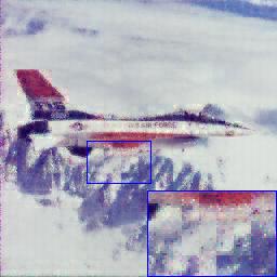
(a) Ket-folding
(24.75dB)

(b) Improved Ket-folding
(25.51dB)

(c) No folding
(22.69dB)

(d) TTC-TV
(23.87dB)

(e) Proposed GraphTT-opt
(26.60dB)

(f) Proposed GraphTT-VI
(29.81dB)

Figure 1: ’airplane’ with $60\%$ missing entries recovered by: (a)-(c). TMAC-TT under different folding strategies, (d) TTC-TV with reshape-folding, (e)-(f) proposed methods without folding.

Size of the folded tensor	TT cores’ total size	Size of matrix to be inverted in each iteration
$[256,256,3,32]$	70912	[65536,65536]
$[4,4,4,4,4,4,4,4,3,8,4]$	3200	[1024,1024]

TABLE I: Comparison between problem sizes for a video tensor with and without folding (max rank set as $16$).

Different from other tensor decompositions, most existing TT/TR methods for image completion are conducted after tensor folding, which folds the 3-dimensional images or 4-dimensional videos to a higher order tensor, e.g., a 9-dimensional tensor. There are two commonly adopted folding strategies. One is ket-folding, or ket augmentation (KA), which was firstly applied in TT format for compressing images [16], and later found to be effective in image completion [11]. This strategy spatially breaks an image or a video into many small blocks, and then use them to fill up a higher order tensor. The other one is reshape-folding, which simply assigns the elements of an image/video tensor sequentially into a higher order tensor. Together with folding, TT/TR based methods achieve the state of the art performance in image completion tasks [11, 17, 14, 15].

While the folding techniques improve the traditional evaluating metrics like PSNR, visual inspection of the recovered images show that they are plagued with heavy ’block effects’. An example is shown in Fig. 1(a), where the recovered ’airplane’ image by TMAC-TT from folded tensor data looks like composing of many small blocks and the edges of the blocks show obvious incoherence. The reason is that tensor folding breaks adjacent pixels into different dimensions. Pixels originally close to each other are assigned to new dimensions and become far away, leading to local information loss. Though an improved folding strategy [14] might help to alleviate the block effect, it is still visible in Fig. 1(b). Futhermore, since the improved folding strategy duplicates the edges of folding blocks, the image size is effectively increased, so does the computational complexity of the algorithm. In comparison, Fig. 1(c) shows the recovered image using the same algorithm as in Fig. 1(a) but without folding. Although some parts of the image are not as clear as that in Fig. 1(a), there is no block effect.

Besides block effect, folding also makes it less efficient to incorporate prior knowledge of image or video like local similarity, which has been widely used to aid visual data recovery, especially in matrix-based methods [18, 19]. After folding, adjacent elements are cast into different dimensions, and the local similarity is only retained within each small block. An example is illustrated in Fig. 1(d), where the recovered ’airplane’ image by the TT completion with total variation regularization (TTC-TV) [17] is shown. Since the TV regularization of TTC-TV only enforces local similarity on each mode of the folded tensor, the block effect is still visible in the image. Surprisingly, the resulting PSNR is even lower than that from TMAC-TT with folding but no local similarity regularization (Fig. 1(a) and Fig. 1(b)).

Given that tensor folding and local similarity are not compatible to each other, one may suggest imposing local similarity but no folding. However, this brings another challenge, which is the large TT/TR core sizes in the model. To understand this clearly, let us focus on the TT format, as it is similar for the TR format. For a tensor of dimensions $[J_{1},\ldots,J_{D}]$ with TT ranks $\{R_{d}\}_{d=1}^{D+1}$, the TT format applied to the original tensor contains totally $\sum_{d=1}^{D}J_{d}R_{d}^{2}$ elements. The problem size is much larger than a folded tensor with number of elements $\sum_{d=1}^{D}\sum_{m=1}^{M}J_{d_{m}}R_{d_{m}}^{2}$ where $J_{d}=\prod_{m=1}^{M}J_{d_{m}}$ if all $R_{d}$ and $R_{d_{m}}$ take similar values, which is often the case. Furthermore, TT completion problems are usually solved in an alternative least squares (ALS) manner, which updates the TT cores iteratively by solving a quadratic sub-problem for each TT core [20, 21, 22]. Due to the correlation induced by the local similarity among slices of the TT cores, an inverse of a $J_{d}R_{d}R_{d+1}\times J_{d}R_{d}R_{d+1}$ matrix is commonly induced in each iteration, which is both space and time comsuming if the tensor is not folded. This is in contrast to TT completion without the local similarity regularization, in which only $J_{d}$ matrices each with size $R_{d}R_{d+1}\times R_{d}R_{d+1}$ are needed to be inverted, since the frontal TT core slices are found to have no correlation with each other [23].

To illustrate these complications, an example is taken from a video tensor with size $256\times 256\times 3\times 32$, where the first $3$ dimensions describe the size of each frame and the last is the number of frames. It can be seen from Table I that without folding, the model size is more than 20 times larger than that with folding, and the matrix to be inverted in each iteration is too large to perform in a personal computer. Even under this modest setting, the algorithms like TTC-TV cannot be executed in a computer with less than $32$GB RAM. In fact, graph regularization on TR decomposition (GNTR) without folding has been attempted in [24]. However, due to the above mentioned high complexity issue, all simulations have been done with very small TR ranks like $3$ or $5$. This might be another reason why most existing TT/TR completion methods involve folding.

	TMAC-TT	SiLRTC-TT	STTO	TTC-TV	TR-VBI	GNTR	GraphTT-opt	GraphTT-VI
No need to fold	✗	✗	✗	✗	✗	not applicable	✓	✓
Graph	✗	✗	✗	✗	✗	✓	✓	✓
Completion	✓	✓	✓	✓	✓	✗	✓	✓
Tuning free	✗	✗	✗	✗	✓	✗	✗	✓

TABLE II: Comparison between existing TT/TR methods and the proposed ones.

In this paper, we focus on the visual data completion problem. As visual data can hardly be accurately represented with very small ranks (e.g., TT/TR with ranks smaller than 10) [15, 17], this brings us to the dilemma: to fold or not to fold. Folding an image or a video tensor would reduce computational complexity but leads to block effect due to local information loss. Not folding a tensor would not lead to block effect and allow us to induce local similarity in the formulation but incur high computational complexity. We propose not to fold the image/video tensor, but use local similarity to boost the completion performance. To overcome the problem of computational complexity, we propose to update each TT core fiber as a unit instead of each TT core. In addition to an optimization based algorithm, a probabilistic model is further built and the corresponding inference algorithm is derived such that no parameter tuning is required. As the key ideas are applicable to both TT and TR completion, in this paper we only focus on the TT completion, and the extension to the TR completion is trivial.

To see the differences between the proposed methods and existing methods, Table II lists various TT/TR completion methods and their modeling characteristics. It can be seen that the proposed methods (GraphTT-opt and GraphTT-VI) are the first ones to embed the graph information into TT completion.

Notice that while a recent work GNTR [24] impose graph regularization to TR without folding, it cannot be directly adopted for the tensor completion tasks as it cannot handle missing data. In addition, as discussed before, it is not applicable for high rank tensor since it does not handle the issue of high computational complexity. Furthermore, it heavily relies on parameter tuning.

The contribution of this paper are summarized as follows.

1. Graph regularization is applied in TT model for image or video completion, with core fibers updated independently in each iteration. This greatly reduces the complexity of tensor core learning.

2. Bayesian modeling and inference algorithm of the above problem are derived. This gets rid of the tideous tuning of TT ranks and regularization parameters.

3. Experiments show the proposed graph-regularized TT completion methods without folding perform better than existing methods while not causing block effect in the recovered data. A sneak preview of the performance of the proposed methods is presented in Fig. 1.

Notation: Boldface lowercase and uppercase letters are used to denote vectors and matrices, respectively. Boldface capital calligraphic letters are used for tensors. $\bm{I}_{n}$ denotes the identity matrix with size $n\times n$. Notation $\text{diag}(\bm{a})$ is a diagonal matrix, with $\bm{a}$ on its diagonal. An element of a matrix or tensor is specified by the subscript, e.g., $\bm{\mathcal{Y}}_{i,j,k}$ denotes the $(i,j,k)$-th element of tensor $\bm{\mathcal{Y}}$, while $\bm{\mathcal{Y}}_{:,:,k}$ includes all elements in the first and second modes with $k$ fixed at the third mode. The operator $\otimes$ denotes the Kronecker product, and $\ast$ denotes the entry-wise product of two tensors with the same size. $\mathbb{E}\llbracket.\rrbracket$ represents the expectation of the variables. $\mathcal{N}(\bm{\mu},\bm{\Sigma})$ denotes the Gaussian distribution with mean vector $\bm{\mu}$ and covariance matrix $\bm{\Sigma}$, and $\text{Gamma}(\alpha,\beta)$ denotes the Gamma distribution with shape $\alpha$ and rate $\beta$.

2 Preliminaries

2.1 Tensor train completion and the ALS solution

In this subsection, we first introduce the tensor train completion problem. Through a sketch of the widely used ALS algorithm, some properties of TT are also introduced, which are important in the proposed algorithms in later sections.

Definition 1 [25]. A $D$-th order tensor $\bm{\mathcal{X}}\in\mathbb{R}^{J_{1}\times J_{2}\times\ldots\times J_{D}}$ is in the TT format if its elements can be expressed as

$$\bm{\mathcal{X}}_{j_{1}j_{2}\ldots j_{D}} =\bm{\mathcal{G}}_{:,:,j_{1}}^{(1)}\bm{\mathcal{G}}_{:,:,j_{2}}^{(2)},\ldots\bm{\mathcal{G}}_{:,:,j_{D}}^{(D)},$$

$$\triangleq\ll\bm{\mathcal{G}}^{(1)},\bm{\mathcal{G}}^{(2)},\ldots,\bm{\mathcal{G}}^{(D)}\gg_{j_{1}j_{2}\ldots j_{D}}$$ (1)

in which $\{\bm{\mathcal{G}}^{(d)}\in\mathbb{R}^{R_{d}\times R_{d+1}\times J_{d}}\}_{d=1}^{D}$ are the TT cores, and $\{R_{d}\}_{d=1}^{D+1}$ are the TT ranks. As can be seen from (1), to express $\bm{\mathcal{X}}_{j_{1}j_{2}\ldots j_{D}}$, the $\{j_{d}\}_{d=1}^{D}$-th frontal slices are selected from the TT cores respectively and then multiplied consecutively. As the product of these slices must be a scalar, $R_{1}$ and $R_{D+1}$ must be $1$. For the other TT ranks $\{R_{d}\}_{d=2}^{D}$, they control the model complexity and are generally unknown.

Suppose $\bm{\mathcal{X}}=\ll\bm{\mathcal{G}}^{(1)},\bm{\mathcal{G}}^{(2)},\ldots,\bm{\mathcal{G}}^{(D)}\gg$ is the tensor to be recovered, and the observed tensor is

$$\bm{\mathcal{Y}}=\bm{\mathcal{O}}\ast(\bm{\mathcal{X}}+\bm{\mathcal{W}}),$$ (2)

where $\bm{\mathcal{W}}$ is a noise tensor which is composed of element-wise independent zero-mean Gaussian noise, and $\bm{\mathcal{O}}$ is an indicator tensor with the same size as $\bm{\mathcal{X}}$ with its element being $1$ if the corresponding element in $\bm{\mathcal{X}}$ is observed, and $0$ otherwise. The basic TT completion problem is formulated as

$$\min_{\bm{\mathcal{G}}^{(1)},\bm{\mathcal{G}}^{(2)},\ldots,\bm{\mathcal{G}}^{(D)}} \left\|\bm{\mathcal{O}}\ast\left(\bm{\mathcal{Y}}-\ll\bm{\mathcal{G}}^{(1)},\bm{\mathcal{G}}^{(2)},\ldots,\bm{\mathcal{G}}^{(D)}\gg\right)\right\|_{F}^{2},$$

s.t. $$\text{TT ranks}=[1,R_{2},\ldots,R_{D},1].$$ (3)

To solve problem (3), ALS is commonly adopted [22, 23], which updates each TT core iteratively until convergence. However, due to the complicatedly coupled tensor cores in the TT format, the following definition and a related property are needed to obtain the solution of each update step.

Definition 2. The mode-$d$ matricization of tensor $\bm{\mathcal{X}}$ is denoted as $\bm{X}_{(d)}\in\mathbb{R}^{J_{d}\times(J_{1}\ldots J_{d-1}J_{d+1}\ldots J_{D})}$, which is obtained by stacking the mode-$d$ fibers $\bm{\mathcal{X}}_{j_{1},\ldots,j_{d-1},:,j_{d+1},\ldots,j_{D}}$ as columns of a matrix. Specifically, the mapping from an element of $\bm{\mathcal{X}}$ to $\bm{X}_{(d)}$ is as follows

$$\bm{\mathcal{X}}_{j_{1}\ldots j_{D}}\rightarrow{\bm{X}_{(d)}}_{j_{d},i},\text{with }{i=j_{1}+\prod_{\begin{subarray}{c}k=2\\ k\neq d\end{subarray}}^{D}\bigg{(}(j_{k}-1)\prod_{\begin{subarray}{c}\ell=1\\ \ell\neq d\end{subarray}}^{k-1}J_{\ell}\bigg{)}}.$$ (4)

Property 1. For tensor $\bm{\mathcal{X}}$ obeying the TT format in (1), its mode-$d$ matricization can be expressed as

$$\bm{X}_{(d)}=\bm{G}_{(3)}^{(d)}\times({\bm{G}_{(1)}^{(>d)}}\otimes{\bm{G}_{(d)}^{(<d)}}),$$ (5)

where $\bm{G}_{(3)}^{(d)}$ is the mode-$3$ matricization of $\bm{\mathcal{G}}^{(d)}$, $\bm{G}_{(d)}^{(<d)}$ is the mode-$d$ matricization of $\bm{\mathcal{G}}^{(<d)}$, with $\bm{\mathcal{G}}^{(<d)}\in\mathbb{R}^{J_{1}\times\ldots\times J_{d-1}\times R_{d}}$ and its element composed by $\bm{\mathcal{G}}_{j_{1},\ldots,j_{d-1},:}^{(<d)}=(\bm{\mathcal{G}}_{:,:,j_{1}}^{(1)}\bm{\mathcal{G}}_{:,:,j_{2}}^{(2)}\ldots\bm{\mathcal{G}}_{:,:,j_{d-1}}^{(d-1)})^{T}$, and $\bm{G}_{(1)}^{(>d)}$ stands for the mode-$1$ unfolding of $\bm{\mathcal{G}}^{(>d)}\in\mathbb{R}^{R_{d+1}\times J_{d+1}\times\ldots\times J_{D}}$, with $\bm{\mathcal{G}}_{:,j_{d+1},\ldots,j_{D}}^{(>d)}=\bm{\mathcal{G}}_{:,:,j_{d+1}}^{(d+1)}\bm{\mathcal{G}}_{:,:,j_{d+2}}^{(d+2)}\ldots\bm{\mathcal{G}}_{:,:,j_{D}}^{(D)}$.

Using Property 1, the subproblem of updating the TT core $\bm{\mathcal{G}}^{(d)}$ can be reformulated as

$$\min_{\bm{\mathcal{G}}^{(d)}}\quad \left\|\bm{O}_{(d)}\ast\bigg{(}\bm{Y}_{(d)}-\bm{G}_{(3)}^{(d)}\times(\bm{G}_{(1)}^{(>d)}\otimes\bm{G}_{(d)}^{(<d)})\bigg{)}\right\|_{F}^{2}$$

$$=\min_{\bm{\mathcal{G}}^{(d)}}\quad \sum_{j_{d}=1}^{J_{d}}\Bigg{\|}{\bm{O}_{(d)}}_{j_{d},:}\ast{\bm{Y}_{(d)}}_{j_{d},:}-{\bm{G}_{(3)}^{(d)}}_{j_{d},:}$$

$$\quad\quad\times\bigg{(}{\bm{O}_{(d)}}_{j_{d},:}\odot(\bm{G}_{(1)}^{(>d)}\otimes\bm{G}_{(d)}^{(<d)})\bigg{)}\Bigg{\|}_{F}^{2}.$$ (6)

From the first line of (6), it is clear that the sub-problem is quadratic with respect to each TT core. Moreover, from the second line of (6) it is worth noticing that different frontal slices from the same TT core $\{{\bm{G}_{(3)}^{(d)}}_{j_{d},:}=\text{vec}(\bm{\mathcal{G}}_{:,:,j_{d}}^{(d)})^{T}\}_{j_{d}=1}^{J_{d}}$ are independent of each other. Thus in each iteration, the solution is obtained by updating its frontal slices in parallel, with

$${\bm{G}_{(3)}^{(d)}}_{j_{d},:}^{T}= {\bigg{(}{\bm{O}_{(d)}}_{j_{d},:}\odot(\bm{G}_{(1)}^{(>d)}\otimes\bm{G}_{(d)}^{(<d)})\bigg{)}^{T}}^{\dagger}$$

$$\quad\quad\quad\times\bigg{(}{\bm{O}_{(d)}}_{j_{d},:}\ast{\bm{Y}_{(d)}}_{j_{d},:}\bigg{)}^{T},$$ (7)

in which the superscript $\dagger$ denotes the Moore-Penrose pseudo inverse.

Since each TT core slice takes the size $R_{d}\times R_{d+1}$, the computational complexity for updating one TT core according to (7) is $\mathcal{O}(R_{d}^{3}R_{d+1}^{3}J_{d})$, and the storage required for the matrix inverse is of $\mathcal{O}(R_{d}^{2}R_{d+1}^{2})$. With high TT ranks, the ALS algorithm would be computationally complicated, which unfortunately is often the case for visual data. This problem would be much more severe when the independence among frontal slices is lost under graph regularization, as will be shown in Section 2.2. Even though matrix inverse can be avoided by gradient method (e.g., STTO [9]), it converges slowly and cannot reduce the storage complexity.

2.2 Graph Laplacian

To introduce smoothness among the entries in a matrix or tensor, graph Laplacian based regularization has recently been widely adopted [26, 19, 27]. For an undirected weighted graph $(\mathcal{V},\mathcal{E})$ with vertices $\mathcal{V}=\{v_{1},\ldots,v_{N}\}$ and the set of edges $\mathcal{E}$, its graph Laplacian is

$$\bm{L}=\bm{D}-\bm{A},$$ (8)

in which $\bm{A}$ is the weight matrix with $\bm{A}_{ij}$ being the weight between $v_{i}$ and $v_{j}$, and $\bm{D}$ is a diagonal matrix with $\bm{D}_{ii}=\sum_{j=1}^{N}A_{ij}$. For a vector $\bm{x}\in\mathbb{R}^{N}$, $\text{tr}(\bm{x}^{T}\bm{L}\bm{x})$ would introduce smoothness among elements of $\bm{x}$ according to $\bm{L}$ since

$$\text{tr}(\bm{x}^{T}\bm{L}\bm{x})=\frac{1}{2}\sum_{i=1}^{N}\sum_{j=1}^{N}\bm{A}_{ij}(\bm{x}_{i}-\bm{x}_{j})^{2}.$$ (9)

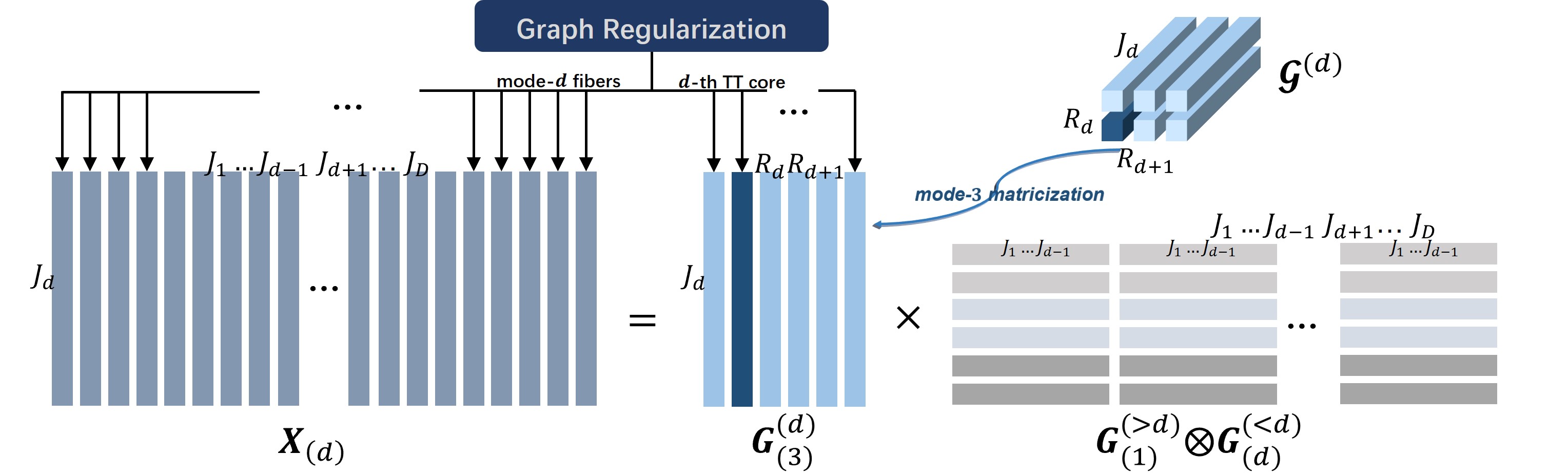
Figure 2: Tensor unfolding and Graph regularization.

To apply the graph regularization (9) in visual data, a direct but naive implementation is to specify the connections between every two entries in the data tensor. However, such method requires a very large graph Laplacian, e.g., a graph Laplacian with size $196008\times 196008$ for a $256\times 256\times 3$ image, which would bring heavy computational burden. Fortunately, from the experience of graph regularized matrix factorization [28, 27], graph information can be added to rows and columns respectively, rather than the vectorization of the matrix. Inspired by this, graph regularization can be applied to each mode of the tensor, or equivalently to the columns of each unfolded tensor $\bm{X}_{(d)}$. The left hand side of Fig. 2 demonstrates this graph embedding. As (5) indicates that mode-$d$ fibers of $\bm{X}$ (i.e., columns of $\bm{X}_{(d)}$) are linear combinations of columns from $\bm{G}_{(3)}^{(d)}$, the regularization that brings local similarity to columns of $\bm{G}_{(3)}^{(d)}$ also promote the local similarity for all mode-$d$ fibers of $\bm{X}$. Therefore, a reasonable graph regularization in the TT format is

$$\quad\text{tr}({\bm{G}_{(3)}^{(d)}}^{T}\bm{L}^{(d)}{\bm{G}_{(3)}^{(d)}})=\sum_{j_{d}=1}^{J_{d}}\sum_{k_{d}=1}^{J_{d}}\bm{L}_{j_{d},k_{d}}^{(d)}{\bm{G}_{(3)}^{(d)}}_{j_{d},:}^{T}{\bm{G}_{(3)}^{(d)}}_{k_{d},:}$$

$$=\sum_{r_{d}=1}^{R_{d}}\sum_{r_{d+1}=1}^{R_{d+1}}{\bm{\mathcal{G}}_{r_{d},r_{d+1},:}^{{(d)}^{T}}}\bm{L}^{(d)}{\bm{\mathcal{G}}_{r_{d},r_{d+1},:}^{(d)}},\text{for }d=1\text{ to }D,$$ (10)

where the second line is due to Definition 2 and it states that graph Laplacian is applied to each fiber of the TT cores. The regularization (10) is depicted in the right hand side of Fig. 2.

On the other hand, it can be observed from Fig. 2 that graph regularization using (10) on the columns of $\bm{G}_{(3)}^{(d)}$ also introduces correlations among frontal slices of the TT core $\bm{\mathcal{G}}^{(d)}$. Thus the update cannot be done in a slice-by-slice manner as in equation (7). If we insist on updating one TT core as a unit in each iteration, the least squares (LS) solution will lead to inversion of a matrix of size $R_{d}R_{d+1}J_{d}\times R_{d}R_{d+1}J_{d}$, which takes time complexity $\mathcal{O}(J_{d}^{3}R_{d}^{3}R_{d+1}^{3})$. Then both the storage and time complexity will be much larger than those required in (7). This makes the algorithm extremely implementation unfridendly. Therefore a new update strategy is required.

In order to model the local similarity of the visual data, it is usually assumed that pixels that are spatially close tend to be similar to each other, leading to a commonly adopted weighting matrices $\bm{A}^{(d)}\in\mathbb{R}^{J_{d}\times J_{d}}$ with element $\bm{A}_{j_{d},k_{d}}^{(d)}=\text{exp}(\alpha|j_{d}-k_{d}|^{2})$, which models the correlation between the $j_{d}$-th row and $k_{d}$-th row of $\bm{X}_{(d)}$, and $\alpha$ is a manually chosen parameter.

3 Graph regularized TT completion with core fiber update

As mentioned in the last section, we use (10) as the graph information to regularize the TT completion problem. This results in the following formulation

$$\min_{\bm{\mathcal{G}}^{(1)},\bm{\mathcal{G}}^{(2)},\ldots,\bm{\mathcal{G}}^{(D)}}\left\|\bm{\mathcal{O}}\ast\left(\bm{\mathcal{Y}}-\ll\bm{\mathcal{G}}^{(1)},\bm{\mathcal{G}}^{(2)},\ldots,\bm{\mathcal{G}}^{(D)}\gg\right)\right\|_{F}^{2}$$

$$\quad\quad\quad+\sum_{d=1}^{D}\beta_{d}{\text{tr}(\bm{G}_{(3)}^{(d)}}^{T}\bm{L}^{(d)}{\bm{G}_{(3)}^{(d)}}),$$

$$\quad s.t.\text{ TT rank}=[1,R_{2},...,R_{D},1],$$ (11)

in which $\bm{L}^{(d)}$ and $\beta_{d}$ are the graph Laplacian and the regularization parameter for the $d$-th mode of the TT model, respectively. If there is no graph information on a particular mode, then the corresponding $\bm{L}^{(d)}$ is set as $\bm{I}_{J_{d}}$, which regularizes the power of $\bm{\mathcal{G}}^{(d)}$ and makes the formulation consistent. Such an regularization is vital since the TT format is invariant by inserting a non-singular matrix among successive TT cores, i.e., $\ll\bm{\mathcal{G}}^{(1)},\ldots,\bm{\mathcal{G}}^{(d)},\bm{\mathcal{G}}^{(d+1)},\ldots,\bm{\mathcal{G}}^{(D)}\gg$ will be the same as $\ll\bm{\mathcal{G}}^{(1)},\ldots,\bar{\bm{\mathcal{G}}}^{(d)},\bar{\bm{\mathcal{G}}}^{(d+1)},\ldots,\bm{\mathcal{G}}^{(D)}\gg$ with $\bar{\bm{G}_{(2)}^{(d)}}^{T}={\bm{G}_{(2)}^{(d)}}^{T}\bm{M}$ and $\bar{\bm{G}_{(1)}^{(d+1)}}=\bm{M}^{-1}{\bm{G}_{(1)}^{(d)}}$. If there is no regularization on a particular TT core $\bm{\mathcal{G}}^{(d)}$, then the other TT cores can transfer their power to this TT core through the aforementioned process and thus all the regularization terms will be close to zero and (11) reduces to the traditional TT completion problem.

To solve problem (11), it is observed that the problem becomes quadratic if we focus on one particular TT core while fixing the others,

$$\min_{\bm{\mathcal{G}}^{(d)}}\left\|\bm{O}_{(d)}\ast\bigg{(}\bm{Y}_{(d)}-\bm{G}_{(3)}^{(d)}\times(\bm{G}_{(1)}^{(>d)}\otimes\bm{G}_{(d)}^{(<d)})\bigg{)}\right\|_{F}^{2}$$

$$\quad\quad\quad+\beta_{d}\text{tr}({\bm{G}_{(3)}^{(d)}}^{T}\bm{L}^{(d)}{\bm{G}_{(3)}^{(d)}})$$ (12)

where various notations were introduced in Section 2.1. Different from the second line of (6) where the frontal slices $\{{\bm{G}_{(3)}^{(d)}}_{j_{d},:}\}_{j_{d}=1}^{J_{d}}$ are independent of each other, the regularization introduces correlation between these slices as reflected in the first line of (10). As discussed in Section 2.2, this would lead to a computationally expensive matrix inverse if we insist on the closed-form update of $\bm{G}_{(3)}^{(d)}$ based on (12).

To bypass this problem, we notice from the second line of (10) that the regularization on $\bm{\mathcal{G}}^{(d)}$ can be separated into $R_{d}R_{d+1}$ independent regularization terms, each of which regularizes a TT core fiber $\bm{\mathcal{G}}_{r_{d},r_{d+1},:}^{(d)}$ (equivalently ${\bm{G}_{(3)}^{(d)}}_{:,p}$ with $p=(r_{d+1}-1)R_{d}+r_{d}$) as a block of variables instead of a TT core. Then, by putting (10) into (12), the problem can be expressed as

$$\min_{\bm{\mathcal{G}}^{(d)}}\bigg{\|}\bm{O}_{(d)}\ast\bigg{(}\bm{Y}_{(d)}-\sum_{p=1}^{R_{d}R_{d+1}}{\bm{G}_{(3)}^{(d)}}_{:,p}\Big{[}\bm{G}_{(1)}^{(>d)}\otimes\bm{G}_{(d)}^{(<d)}\Big{]}_{p,:}\bigg{)}\bigg{\|}_{F}^{2}$$

$$\quad\quad\quad+\beta_{d}\sum_{p=1}^{R_{d}R_{d+1}}{\bm{G}_{(3)}^{(d)}}_{:,p}^{T}\bm{L}^{(d)}{\bm{G}_{(3)}^{(d)}}_{:,p},$$ (13)

Focusing on the terms that are only related to ${\bm{G}_{(3)}^{(d)}}_{:,p}$, (13) simplifies to

$$\min_{{\bm{G}_{(3)}^{(d)}}_{:,p}}\Bigg{\|}\bm{O}_{(d)}\ast\bigg{(}\bm{Y}_{(d)}-\sum_{q=1,q\neq p}^{R_{d}R_{d+1}}{\bm{G}_{(3)}^{(d)}}_{:,q}\Big{[}\bm{G}_{(1)}^{(>d)}\otimes\bm{G}_{(d)}^{(<d)}\Big{]}_{q,:}\bigg{)}$$

$$\quad\quad\quad-\bm{O}_{(d)}\ast\big{(}{\bm{G}_{(3)}^{(d)}}_{:,p}\Big{[}\bm{G}_{(1)}^{(>d)}\otimes\bm{G}_{(d)}^{(<d)}\Big{]}_{p,:}\big{)}\Bigg{\|}_{F}^{2}$$

$$\quad\quad\quad+\beta_{d}{\bm{G}_{(3)}^{(d)}}_{:,p}^{T}\bm{L}^{(d)}{\bm{G}_{(3)}^{(d)}}_{:,p},$$ (14)

which is quadratic with respect to the TT core fiber ${\bm{G}_{(3)}^{(d)}}_{:,p}$, and the closed-form solution is shown in Appendix A to be

$${\bm{G}_{(3)}^{(d)}}_{:,p}={\bm{\Upsilon}^{(d,p)}}^{-1}{\bm{\mu}^{(d,p)}},$$ (15)

with

$$\bm{\Upsilon}^{(d,p)}=\text{diag}\bigg{(}\bm{O}_{(d)}(\Big{[}\bm{G}_{(1)}^{(>d)}\otimes\bm{G}_{(d)}^{(<d)}\Big{]}_{p,:}^{T}$$

$$\quad\quad\quad\quad\quad\ast\Big{[}\bm{G}_{(1)}^{(>d)}\otimes\bm{G}_{(d)}^{(<d)}\Big{]}_{p,:}^{T})\bigg{)}+\beta_{d}\bm{L}^{(d)},$$ (16)

$$\bm{\mu}^{(d,p)}=\bigg{(}\bm{O}_{(d)}\ast\Big{(}\bm{Y}_{(d)}-\sum_{q=1,q\neq p}^{R_{d}R_{d+1}}{\bm{G}_{(3)}^{(d)}}_{:,q}$$

$$\quad\quad\times\Big{[}\bm{G}_{(1)}^{(>d)}\otimes\bm{G}_{(d)}^{(<d)}\Big{]}_{q,:}\Big{)}\bigg{)}\Big{[}\bm{G}_{(1)}^{(>d)}\otimes\bm{G}_{(d)}^{(<d)}\Big{]}_{p,:}^{T}.$$ (17)

The whole algorithm, which solves (11) using the ALS, is shown in Algorithm 1. For a particular TT core, the basic LS problem in (14) is solved from $p=1$ to $R_{d}R_{d+1}$. Then various TT cores are updated from $d=1$ to $D$ at the outer iteration.

Algorithm 1 is in block coordinate descent (BCD) framework for solving (11), in which each subproblem is solving for a TT core fiber. Since each subproblem is quadratic, (15) is the global optimal solution to each subproblem, and therefore Algorithm 1 converges to a stationary point of (11) [29]. Notice that even if we choose to update a whole TT core as a block of variables, the corresponding algorithm is still under the BCD framework, and the convergent point is still a stationary point of (11). In this sense, while updating each TT core and updating each TT core fiber in the BCD lead to different solutions, they achieves the same quality of convergent point. Experiments on synthetic data will be provided to compare the two updating mechanisms in Section 5.1, which show the proposed fiber update using (14) performs similarly to the core update based on (12).

For a fiber from the $d$-th TT core, it takes around $\bm{O}({J_{d}}^{3})$ to compute the solution to (14). Apart from that, it takes around $\bm{O}(R^{4}\prod_{k=1}^{D}J_{k})$ to obtain $\bm{\Upsilon}^{(d,p)}$ and $\bm{\mu}^{(d)}$. Since there are common terms for different fibers in the same TT core, in general it takes complexity $\bm{O}(R^{2}{J_{d}}^{3}+R^{4}\prod_{k=1}^{D}J_{k})$ for the update of each TT core. In contrast, if we update one TT core as a whole, it would take $\bm{O}(R^{6}J_{d}^{3}+R^{4}\prod_{k=1}^{D}J_{k})$ to compute the closed-form solution, which is much more complicated. Furthermore, the storage complexity required for the matrix to be inverted is $\bm{O}(R^{4}J_{d}^{2})$ for the core update, while that of the proposed algorithm is only $\bm{O}(J_{d}^{2})$. Suppose we use $64$-bit double type data, with $J_{d}=256$ and $R_{d}=R_{d+1}=16$, then the amount of RAM required for the matrix in the core update is $32$GB, while the proposed fiber update only requires $512$KB.

initialization: Input the observed tensor $\bm{\mathcal{Y}}$ and indicator tensor $\bm{\mathcal{O}}$. Set TT ranks $\{R_{d}\}_{d=1}^{D+1}$, the graph Laplacian $\{\bm{L}^{(d)}\}_{d=1}^{D}$, and regularization parameters $\{\bm{\beta}_{d}\}_{d=1}^{D}$;

while Not Converged do

       For $d=1$ to $D-1$

       For $p=1$ to $R_{d}R_{d+1}$

        Update ${\bm{G}_{(3)}^{(d)}}_{:,p}$ according to (15);

       end

      end

end while

Algorithm 1 TT completion with graph regularization (GraphTT-opt).

4 A Bayesian treatment to graph TTC

In the last section, Algorithm 1 is provided to solve the graph regularized TT completion problem. However, a critical drawback of Algorithm 1 is that it heavily relies on parameter tuning, like most optimization based methods do. For TT completion with graph regularization, the burden of parameter tuning is even heavier than that of traditional matrix completion or canonical polyadic (CP) completion, since the TT model has multiple TT ranks, and for each TT core there is an individual regularization parameter for the graph information. For example, for a $4$-th order tensor $\bm{\mathcal{Y}}$, there are $3$ TT-ranks and $4$ graph regularization parameters to be tuned.

To solve this problem, probabilistic model, which has shown its ability to perform matrix/tensor completion without the need of parameter tuning [30, 31, 32, 14], is adopted in this section.

4.1 The generalized hyperbolic model for TT with graph information embedding

Firstly, from (2), due to the additive white Gaussian noise, the log likelihood of the observed tensor $\bm{\mathcal{Y}}$ is

$$\ln{\left(p(\bm{\mathcal{Y}}|\bm{\mathcal{O}},\{\bm{\mathcal{G}}^{(d)}\}_{d=1}^{D},\tau)\right)}=\frac{|\Omega|}{2}\ln{\tau}-\frac{\tau}{2}\Big{\|}\bm{\mathcal{O}}\ast\big{(}\bm{\mathcal{Y}}$$

$$\quad\quad-\ll\bm{\mathcal{G}}^{(1)},\bm{\mathcal{G}}^{(2)},\ldots,\bm{\mathcal{G}}^{(D)}\gg\big{)}\Big{\|}_{F}^{2}+\text{const},$$ (18)

where $\tau$ is the inverse of the noise variance, $\Omega$ denotes the set of indices of the observed entries, and $|\Omega|$ denotes the cardinality of $\Omega$, which equals the number of observed entries. For the noise precision $\tau$, it is assumed to follow a Gamma distribution as

$$p(\tau|{\alpha}_{\tau},{\beta}_{\tau})=\text{Gamma}(\tau|{\alpha}_{\tau},{\beta}_{\tau}).$$ (19)

To enable estimation of the TT-ranks during inference, a sparsity inducing prior distribution with graph information is adopted for each TT core

$$\quad p(\bm{\mathcal{G}}^{(d)}|\bm{z}^{(d)},\bm{z}^{(d+1)})=$$

$$\prod_{k=1}^{S_{d}}\prod_{\ell=1}^{S_{d+1}}\mathcal{N}\Big{(}\bm{\mathcal{G}}_{k,\ell,:}^{(d)}|\bm{0},\bm{z}_{k}^{(d)}\bm{z}_{\ell}^{(d+1)}{\bm{L}^{(d)}}^{-1}\Big{)},\forall d\in\{1,\ldots,D\},$$ (20)

$$p(\bm{z}^{(d)}|\bm{a}^{(d)},\bm{b}^{(d)},\bm{\lambda}^{(d)})=\prod_{k=1}^{S_{d}}\text{GIG}(\bm{z}_{k}^{(d)}|\bm{a}_{k}^{(d)},\bm{b}_{k}^{(d)},\bm{\lambda}_{k}^{(d)}),$$

$$\quad\quad\quad\quad\forall d\{2,\ldots,D\},$$ (21)

where $S_{d}$ and $S_{d+1}$ are upper bound of $R_{d}$ and $R_{d+1}$ respectively [7, 33], which are set as large numbers in practice so that learning the TT ranks in the inference algorithm is possible. $\bm{z}^{(d)}=[\bm{z}_{1}^{(d)},\ldots,\bm{z}_{S_{d}}^{(d)}]$ controls the variance of all mode-$3$ fibers in both $\mathcal{G}^{(d)}$ and $\mathcal{G}^{(d+1)}$. In particular, $\bm{z}^{(1)}$ and $\bm{z}^{(D+1)}$ are scalars and set as $1$ so that the expression in (20) is applicable for the first and last TT cores. As in (21), each element of $\bm{z}^{(d)}$ is modeled to follow a generalized inverse Gaussian (GIG) distribution, which is controlled by the hyperparameters $\bm{a}^{(d)},\bm{b}^{(d)},\bm{\lambda}^{(d)}$ and is defined as

$$\text{GIG}(\bm{z}_{k}^{(d)}|\bm{a}_{k}^{(d)},\bm{b}_{k}^{(d)},\bm{\lambda}_{k}^{(d)})=\frac{(\frac{\bm{a}_{k}^{(d)}}{\bm{b}_{k}^{(d)}})^{\frac{\bm{\lambda}_{k}^{(d)}}{2}}}{2K_{\bm{\lambda}_{k}^{(d)}}(\sqrt{\bm{a}_{k}^{(d)}\bm{b}_{k}^{(d)}})}{\bm{z}_{k}^{(d)}}^{\bm{\lambda}_{k}^{(d)}-1}$$

$$\quad\quad\quad\times\text{exp}\Bigg{(}-\frac{1}{2}(\bm{a}_{k}^{(d)}\bm{z}_{k}^{(d)}+\bm{b}_{k}^{(d)}\frac{1}{\bm{z}_{k}^{(d)}})\Bigg{)},$$ (22)

where $K_{.}(.)$ is the modified Bessel function of the second kind. For $\bm{a}^{(d)}$ which dominantly affects the distribution of $\bm{z}^{(d)}$, it is further assigned a Gamma distribution as

$$p(\bm{a}^{(d)}|\bm{c}^{(d)},\bm{f}^{(d)})=\text{Gamma}(\bm{c}^{(d)},\bm{f}^{(d)}).$$ (23)

Previous Bayesian TT model [14] makes use of traditional Gaussian-Gamma model. Recently, GIG model has been shown to outperforms Gaussian-Gamma model in the context of CP decomposition, especially in low signal-to-noise ratio (SNR) and high rank scenario [34]. The model (19)-(23) is an extension of GIG model to the problem of TT completion. Furthermore, graph regularization is included in (20), which has not been done in Bayesian TT modeling before.

4.2 Inference algorithm

Given the probabilistic model (19)-(23), we need to infer the unknown variables $\bm{\Theta}:=\big{\{}\{\bm{\mathcal{G}}^{(d)}\}_{d=1}^{D},\{\bm{z}^{(d)}\}_{d=2}^{D},\{\bm{a}^{(d)}\}_{d=2}^{D},$ $\tau\big{\}}$ based on the observation $\bm{\mathcal{Y}}$. In Bayesian inference, this is achieved through the posterior distribution $p(\bm{\Theta}|\bm{\mathcal{Y}})=p(\bm{\mathcal{Y}},\bm{\Theta})/p(\bm{\mathcal{Y}})$. However, the Bayesian graph-regularized TT model is so complicated that there is no closed-form expression for $p(\bm{\mathcal{Y}})=\int p(\bm{\mathcal{Y}},\bm{\Theta})d\bm{\Theta}$, and therefore the posterior distribution $p(\bm{\Theta}|\bm{\mathcal{Y}})$ cannot be computed explicitly. Therefore, instead of directly deriving the posterior distribution, variational inference (VI) is adopted, which tries to find a variational distribution $q(\bm{\Theta})$ that best approximate the posterior distribution by minimizing the Kullback-Leibler (KL) divergence

$$\min_{q(\bm{\Theta})}\text{ KL}\bigg{(}q(\bm{\Theta})\text{ }||\text{ }p(\bm{\Theta}|\bm{\mathcal{Y}})\bigg{)}=\int q(\bm{\Theta})\ln\frac{q(\bm{\Theta})}{p(\bm{\Theta}|\bm{\mathcal{Y}})}\text{d}\bm{\Theta}.$$ (24)

To solve (18), mean-field approximation is commonly adopted, which assumes that $q(\bm{\Theta})=\prod_{s=1}^{S}q(\bm{\Theta}_{s})$, where $\{\bm{\Theta}_{s}\}_{s=1}^{S}$ are non-overlapping partitioning of $\bm{\Theta}$ (i.e. $\bm{\Theta}_{s}\subset\bm{\Theta}$, $\cup_{s=1}^{S}\bm{\Theta}_{s}=\bm{\Theta}$, and $\bm{\Theta}_{s}\cap\bm{\Theta}_{t}=\emptyset$ for $s\neq t$). Under the mean-field approximation, the optimal solution for $\bm{\Theta}_{s}$ (when other variables are fixed) can be derived as [35, pp. 737]

$$\ln{q^{*}({\bm{\Theta}}_{s})}=\mathbb{E}_{\bm{\Theta}\backslash{\bm{\Theta}}_{s}}\llbracket\ln{p(\bm{\mathcal{Y}},\bm{\Theta})}\rrbracket+\text{const},$$ (25)

where $\mathbb{E}_{\bm{\Theta}\backslash{\bm{\Theta}}_{s}}\llbracket.\rrbracket$ denotes the expectation over all variables expect $\bm{\Theta}_{s}$. For the proposed TT model, we employ the mean-field

$$q(\bm{\Theta})=\prod_{d=1}^{D}\prod_{k=1}^{S_{d}}\prod_{\ell=1}^{S_{d+1}}q(\bm{\mathcal{G}}_{k,\ell,:}^{(d)})\prod_{d=2}^{D}q(\bm{z}^{(d)})\prod_{d=2}^{D}q(\bm{a}^{(d)})q(\tau).$$ (26)

Under this mean-field approximation, the optimal variational distributions of different variables are derived using (25) with $p(\bm{\mathcal{Y}},\bm{\Theta})=p(\bm{\mathcal{Y}}|\bm{\mathcal{O}},\{\bm{\mathcal{G}}^{(d)}\}_{d=1}^{D},\tau)$ $\prod_{d=1}^{D}p(\bm{\mathcal{G}}^{(d)})$ $\prod_{d=1}^{D}p(\bm{z}^{(d)})$ $\prod_{d=1}^{D}p(\bm{a}^{(d)})p(\tau)$. The detailed derivations are given in Appendix B and the results are presented below.

Update $\bm{{G}}_{:,p}^{(d)}$ for $p$ from $1$ to $S_{d}S_{d+1}$, $d$ from $1$ to $D$

For each fiber of $\bm{\mathcal{G}}^{(d)}$, its variational distribution follows a Gaussian distribution

$$q(\bm{G}_{:,p}^{(d)})=\mathcal{N}(\bm{\nu}^{(d,p)},\bm{\Sigma}^{(d,p)}),$$

with

$$\bm{\Sigma}^{(d,p)}=\Bigg{(}\mathbb{E}{\big{\llbracket}\tau\big{\rrbracket}}\text{diag}\bigg{(}\bm{O}_{(d)}\mathbb{E}\bigg{\llbracket}\Big{[}\bm{G}_{(1)}^{(>d)}\otimes\bm{G}_{(d)}^{(<d)}\Big{]}_{p,:}^{T}$$

$$\ast\Big{[}\bm{G}_{(1)}^{(>d)}\otimes\bm{G}_{(d)}^{(<d)}\Big{]}_{p,:}^{T}\bigg{\rrbracket}\bigg{)}+\mathbb{E}\bigg{\llbracket}\frac{1}{\bm{z}_{k_{p}}^{(d)}}\bigg{\rrbracket}\mathbb{E}\bigg{\llbracket}\frac{1}{\bm{z}_{\ell_{p}}^{(d+1)}}\bigg{\rrbracket}\bm{L}^{(d)}\Bigg{)}^{-1},$$ (27)

$$\bm{\nu}^{(d,p)}=\mathbb{E}{\big{\llbracket}\tau\big{\rrbracket}}\bm{\Sigma}^{(d,p)}\bigg{(}\Big{(}\bm{O}_{(d)}\ast\bm{Y}_{(d)}\Big{)}\mathbb{E}\bigg{\llbracket}\Big{[}\bm{G}_{(1)}^{(>d)}\otimes\bm{G}_{(d)}^{(<d)}\Big{]}_{p,:}^{T}\bigg{\rrbracket}$$

$$-\sum_{q=1,q\neq p}^{S_{d}S_{d+1}}\text{diag}\Big{(}\mathbb{E}\Big{\llbracket}{\bm{G}_{(3)}^{(d)}}_{:,q}\Big{\rrbracket}\Big{)}\bm{O}_{(d)}\mathbb{E}\bigg{\llbracket}\Big{[}\bm{G}_{(1)}^{(>d)}\otimes\bm{G}_{(d)}^{(<d)}\Big{]}_{q,:}^{T}$$

$$\ast\Big{[}\bm{G}_{(1)}^{(>d)}\otimes\bm{G}_{(d)}^{(<d)}\Big{]}_{p,:}^{T}\bigg{\rrbracket}\bigg{)}.$$ (28)

Most of the expectations in (27) and (28) are trivial, except $\mathbb{E}\llbracket[\bm{G}_{(1)}^{(>d)}\otimes\bm{G}_{(d)}^{(<d)}]_{q,:}^{T}\ast[\bm{G}_{(1)}^{(>d)}\otimes\bm{G}_{(d)}^{(<d)}]_{p,:}^{T}\rrbracket$, which is discussed in detail in Appendix B.

Update $\bm{a}^{(d)}$ from $d=2$ to $D$

For $\bm{a}^{(d)}$, it follows a Gamma distribution

$$p(\bm{a}^{(d)}|\hat{\bm{c}}_{k}^{(d)},\hat{\bm{f}}_{k}^{(d)})=\prod_{k=1}^{S_{d}}\text{Gamma}(\bm{a}_{k}^{(d)}|\hat{\bm{c}}_{k}^{(d)},\hat{\bm{f}}_{k}^{(d)}),$$

with

$$\hat{\bm{c}}_{k}^{(d)}=\bm{c}_{k}^{(d)}+\frac{\hat{\bm{\lambda}}_{k}^{(d)}}{2},$$ (29)

$$\hat{\bm{f}}_{k}^{(d)}=\bm{f}_{k}^{(d)}+\frac{\mathbb{E}[\bm{z}_{k}^{(d)}]}{2}.$$ (30)

initialization: Input the observed tensor $\bm{\mathcal{Y}}$. Set initial ranks $\{S_{d}\}_{d=1}^{D}$ and hyperparameters $\{\bm{\lambda}^{(d)}\}_{d=2}^{D}$, $\{\bm{b}^{(d)}\}_{d=2}^{D}$, $\{\bm{c}^{(d)}\}_{d=2}^{D}$, $\{\bm{f}^{(d)}\}_{d=2}^{D}$, $\alpha_{\tau}$, $\beta_{\tau}$;

while Not Converged do

       Update $q(\bm{G}_{:,p}^{(d)})$ via (27) and (28) sequentially for $p=1,\ldots,S_{d}S_{d+1}$ and $d=1,\ldots,D$;

       Update $\{q(\bm{a}^{(d)})\}_{d=2}^{D}$ via (29), (30) sequentially for $d=2,\dots,D$;

       Update $\{q(\bm{z}^{(d)})\}_{d=2}^{D}$ via (31), (32) and (33) sequentially for $d=2,\dots,D$;

       Update $q(\tau)$ via (34) and (35);

       Rank selection;

      

end while

Algorithm 2 VI Algorithm for the probabilistic graph regularized TT model (GraphTT-VI).

Update $\bm{z}^{(d)}$ from $d=2$ to $D$

The variational distribution of $\bm{z}^{(d)}$ follows a GIG distribution

$$p(\bm{z}^{(d)}|\hat{\bm{a}}^{(d)},\hat{\bm{b}}^{(d)},\hat{\bm{\lambda}}^{(d)})=\prod_{k=1}^{S_{d}}\text{GIG}(\bm{z}_{k}^{(d)}|\hat{\bm{a}}^{(d)},\hat{\bm{b}}^{(d)},\hat{\bm{\lambda}}^{(d)}),$$

with the parameters updated as

$$\hat{\bm{a}}_{k}^{(d)}=\mathbb{E}\big{\llbracket}{\bm{a}_{k}^{(d)}}\big{\rrbracket},$$ (31)

$$\hat{\bm{\lambda}}_{k}^{(d)}=\bm{\lambda}_{k}^{(d)}-\frac{J_{d}S_{d+1}}{2}-\frac{J_{d-1}S_{d-1}}{2},$$ (32)

$$\hat{\bm{b}}_{k}^{(d)}=\bm{b}_{k}^{(d)}+\frac{1}{2}\sum_{\ell=1}^{S_{d-1}}\mathbb{E}\big{\llbracket}\frac{1}{\bm{z}_{\ell}^{(d-1)}}\big{\rrbracket}\mathbb{E}\big{\llbracket}{\bm{\mathcal{G}}_{\ell,k,:}^{(d-1)}}^{T}\bm{L}^{(d-1)}{\bm{\mathcal{G}}_{\ell,k,:}^{(d-1)}}\big{\rrbracket}$$

$$+\sum_{\ell=1}^{S_{d+1}}\mathbb{E}\big{\llbracket}\frac{1}{\bm{z}_{\ell}^{(d+1)}}\big{\rrbracket}\mathbb{E}\llbracket{\bm{\mathcal{G}}_{\ell,k,:}^{(d)}}^{T}\bm{L}^{(d)}{\bm{\mathcal{G}}_{\ell,k,:}^{(d)}}\rrbracket.$$ (33)

TABLE III: Calculation of Expectations.

Expectations	Calculation
$\mathbb{E}\llbracket\bm{\mathcal{G}}_{k,\ell,:}^{(d)}\rrbracket,\forall k,\ell,d$	$\bm{\nu}^{(d,(\ell-1)S_{d}+k)},\forall k,\ell,d$
$\mathbb{E}\llbracket{\bm{\mathcal{G}}_{:,:,j_{d}}^{(d)}\otimes\bm{\mathcal{G}}_{:,:,j_{d}}^{(d)}}\rrbracket,\forall d,j_{d}$	$\bm{\mathrm{Var}}^{(d,j_{d})}+\mathbb{E}\big{\llbracket}\bm{\mathcal{G}}_{:,:,j_{d}}^{(d)}\big{\rrbracket}\otimes\mathbb{E}\big{\llbracket}\bm{\mathcal{G}}_{:,:,j_{d}}^{(d)}\big{\rrbracket}$, with $\quad\quad\bm{\mathrm{Var}}_{i,t}^{(d,j_{d})}=\begin{cases}\bm{\Sigma}_{j_{d},j_{d}}^{(d,(\ell-1)S_{d}+k)},&\text{if }i\in\{(k-1)S_{d}+k\}_{k=1}^{S_{d}}\\ \quad&\&\quad t\in\{(\ell-1)S_{d+1}+\ell\}_{\ell=1}^{S_{d+1}}\\ 0,&\text{otherwise}\end{cases}$
$\mathbb{E}\llbracket\bm{z}_{k}^{(d)}\rrbracket,\forall k,d$	$\left(\frac{\hat{\bm{b}}_{k}^{(d)}}{\hat{\bm{a}}_{k}^{(d)}}\right)^{\frac{1}{2}}\frac{K_{\hat{\bm{\lambda}}_{k}^{(d)}+1}\left(\sqrt{\hat{\bm{a}}_{k}^{(d)}\hat{\bm{b}}_{k}^{(d)}}\right)}{K_{\hat{\bm{\lambda}}_{k}^{(d)}}\left(\hat{\bm{a}}_{k}^{(d)}\hat{\bm{b}}_{k}^{(d)}\right)}$
$\mathbb{E}\big{\llbracket}\frac{1}{\bm{z}_{k}^{(d)}}\big{\rrbracket},\forall k,d$	$\left(\frac{\hat{\bm{b}}_{k}^{(d)}}{\hat{\bm{a}}_{k}^{(d)}}\right)^{-\frac{1}{2}}\frac{K_{\hat{\bm{\lambda}}_{k}^{(d)}+1}\left(\sqrt{\hat{\bm{a}}_{k}^{(d)}\hat{\bm{b}}_{k}^{(d)}}\right)}{K_{\hat{\bm{\lambda}}_{k}^{(d)}-1}\left(\hat{\bm{a}}_{k}^{(d)}\hat{\bm{b}}_{k}^{(d)}\right)}$
$\mathbb{E}\llbracket\bm{a}_{k}^{(d)}\rrbracket,\forall k,d$	${\hat{\bm{c}}_{k}^{(d)}}/{\hat{\bm{f}}_{k}^{(d)}}$
$\mathbb{E}\llbracket\tau\rrbracket$	${\hat{\alpha}_{\tau}}/{\hat{\beta}_{\tau}}$

Update $\tau$

The variational distribution of $\tau$ follows a Gamma distribution

$$q(\tau)=\text{Gamma}(\hat{\alpha}_{\tau},\hat{\beta}_{\tau}),$$

with parameters

$$\hat{\alpha}_{\tau}=\alpha_{\tau}+\frac{|\Omega|}{2},$$ (34)

and

$$\hat{\beta}_{\tau}=\beta_{\tau}+\frac{1}{2}\bigg{(}\left\|\bm{\mathcal{O}}\ast\bm{\mathcal{Y}}\right\|_{F}^{2}-2\sum_{j_{1}=1}^{J_{1}}\ldots\sum_{j_{D}=1}^{J_{D}}\bm{\mathcal{O}}_{j_{1}\ldots j_{D}}\bm{\mathcal{Y}}_{j_{1}\ldots j_{D}}$$

$$\times\mathbb{E}\llbracket\bm{\mathcal{G}}_{:,:,j_{1}}^{(1)}\rrbracket\ldots\mathbb{E}\llbracket\bm{\mathcal{G}}_{:,:,j_{D}}^{(D)}\rrbracket+\sum_{j_{1}=1}^{J_{1}}\ldots\sum_{j_{D}=1}^{J_{D}}\bm{\mathcal{O}}_{j_{1}\ldots j_{D}}$$

$$\times\mathbb{E}\llbracket\bm{\mathcal{G}}_{:,:,j_{1}}^{(1)}\otimes\bm{\mathcal{G}}_{:,:,j_{1}}^{(1)}\rrbracket\ldots\mathbb{E}\llbracket\bm{\mathcal{G}}_{:,:,j_{D}}^{(D)}\otimes\bm{\mathcal{G}}_{:,:,j_{D}}^{(D)}\rrbracket\bigg{)}.$$ (35)

As updating a certain $q(\bm{\Theta}_{s})$ requires the statistics of other $\{\bm{\Theta}_{k}\}_{k\neq s}$, various variational distributions are updated iteratively. The proposed Bayesian algorithm is summarized in Algorithm 2, and the required expectations are given in Table. III.

4.3 Further discussions

Insights of the VI updates. To give an insight on how the proposed algorithm works, we firstly see how (25) is expressed with respect to a TT core fiber, which follows a quadratic form

$$\ln{q^{*}({\bm{G}_{:,p}^{(d)}})}=\mathbb{E}_{\backslash{\bm{G}_{:,p}^{(d)}}}\bigg{\llbracket}\tau\bigg{\|}\bm{O}_{(d)}\ast\bigg{(}\bm{Y}_{(d)}-\bm{G}_{(3)}^{(d)}\times(\bm{G}_{(1)}^{(>d)}$$

$$\otimes\bm{G}_{(d)}^{(<d)})\bigg{)}\bigg{\|}_{F}^{2}+\frac{1}{\bm{z}_{k_{p}}^{(d)}\bm{z}_{\ell_{p}}^{(d+1)}}\text{tr}({\bm{G}_{(3)}^{(d)}}_{:,p}^{T}\bm{L}^{(d)}{\bm{G}_{(3)}^{(d)}}_{:,p})\bigg{\rrbracket}.$$ (36)

Since $q^{*}(\bm{G}_{:,p}^{(d)})$ follows a Gaussian distribution, the minimum value of $\ln{q^{*}({\bm{G}_{:,p}^{(d)}})}$ w.r.t. $\bm{G}_{:,p}^{(d)}$ is exactly attained when $\bm{G}_{:,p}^{(d)}=\bm{\nu}^{(d,p)}$. Furthermore, as $\{\bm{\nu}^{(d,p)}\}_{p=1,d=1}^{R_{d}R_{d+1},D}$ will be adopted to reconstruct the tensor after the convergence of Algorithm 2, the VI update using (36) is similar to the minimization problem (12) w.r.t. ${\bm{G}_{:,p}^{(d)}}$, except the expectation and different coefficients in (36). For the ’coefficients’ in (36), they are actually modeled as variables and are updated adaptively as shown in Algorithm 2, which takes into consideration the noise level $\tau$ and the weighted TT core slice power $\{\bm{z}_{d}\}_{d=2}^{D}$, and thus in turns refines (36) to better model the observed data. In contrast, the coefficients in (12) are all fixed and do not have the ability to adapt to different types of data, e.g., different noise or missing ratio, as will be seen in various experiments in Section. 5.

Rank Selection. The proposed probabilistic TT model has the ability to introduce sparsity into the vertical and horizontal slices of the TT cores [34, 14]. Even with graph Laplacian included, it has recently been proved that such model is also sparsity promoting [27]. After the iterative VI updates, the sparsity inducing variables $\{\bm{z}^{(d)}\}_{d=2}^{(D)}$ tend to have a variational distribution under which many $\mathbb{E}\llbracket{\bm{z}_{k}^{(d)}}\rrbracket$ are close to $0$, and thus the corresponding $\mathbb{E}\llbracket\frac{1}{\bm{z}_{k}^{(d)}}\rrbracket$ have very large values. On the other hand, it can be seen from (27) that a large $\mathbb{E}\llbracket\frac{1}{\bm{z}_{k_{p}}^{(d)}}\rrbracket$ would lead the elements of the corresponding $\bm{\Sigma}^{(d,p)}$ and $\bm{\Sigma}^{(d-1,p)}$ to be very samll, and therefore lead all the elements in the expectation $\bm{\nu}^{(d,p)}$ and $\bm{\nu}^{(d-1,p)}$ close to zero. In this way group sparsity is introduced and thus the TT-ranks can be automatically determined. In practice, if the power of $\bm{\mathcal{G}}_{:,k,:}^{(d)}$ and $\bm{\mathcal{G}}_{k,:,:}^{(d+1)}$ both tend to be $0$, e.g., less than $1e^{-7}$, these two slices can be discarded.

Convergence Analysis. The convergence of Algorithm 2 is guaranteed, as it has been proved that (24) is convex with respect to each variable set $\bm{\Theta}_{s}$ under the mean-field approximation [36, pp. 466]. As (25) is the optimal solution to (24) w.r.t. $\bm{\Theta}_{s}$, the KL divergence between the true posterior and the variational distribution is non-increasing after each update. Moreover, the rank pruning can be performed after every iteration with the convergence property preserved, since every time a slice is deleted, it is equivalent to restarting the VI algorithm with a smaller model size and with the current variational distribution serving as a new initialization.

Complexity Analysis. Algorithm 2 uses most of time on updating the variational distributions of the TT cores. For the updates of other variables $\{\bm{z}^{(d)}\}_{d=2}^{D}$, $\{\bm{a}^{(d)}\}_{d=2}^{D}$ and $\tau$, they either are with simple expressions or can re-use computation results required for the TT core update. For each TT core fiber, it takes $\bm{O}({J_{d}^{3}}+{R^{4}|\Omega|})$ to obtain (27) and (28). By noticing that there are unchanged factors for different fibers in (27) and (28), the total complexity for updating one TT core is $\bm{O}\left(R^{2}|\Omega|+R^{4}J_{d}^{3}\right)$. Then for an iteration of Algorithm 2, it takes computational complexity $\bm{O}\left(DR^{2}|\Omega|+DR^{4}J_{d}^{3}\right)$.

5 Experiments

In this section, the performance of the proposed algorithms will be tested on both synthetic and real-world data. In experiments on synthetic data, the effects of the parameters like initial ranks and regularization parameters will be tested under different noise and missing rates. The convergence performance of GraphTT-opt with fiber update is also compared to that with core update as in (12). In the real-world experiment, different kinds of datasets, including images and videos, are tested under different noise and missing patterns. For comparison, the performance of some state-of-the-art methods will also be provided.

For the initialization of the proposed methods, we first fill in the missing entries through i.i.d. Gaussian distributed variables with mean and variance obtained from the observed data. Then TT-SVD is performed with truncated TT-ranks set as the initialized ranks, and the initial TT cores $\{\bm{\mathcal{G}}_{0}^{(d)}\}_{d=1}^{D}$ are obtained. For the regularization parameters, we choose to set only $\beta_{0}$ to better illustrate its effects on the optimization based algorithm. To balance the regularization on each mode, $\beta_{d}$ is accordingly set as $\beta_{0}/\text{tr}({{\bm{G}_{0}}_{(3)}^{(d)}}^{T}{\bm{G}_{0}}_{(3)}^{(d)})$, where ${\bm{G}_{0}}_{(3)}^{(d)}$ is the mode-$3$ unfolding of the $d$-th initialized TT core $\bm{\mathcal{G}}_{0}^{(d)}$. For the initialization of the compared methods, they are fine-tuned around the parameter setting introduced in the original works to the best performance.

5.1 Comparing fiber update vs. core update in synthetic data

In this subsection, we use synthetic data to test the performance of the proposed algorithms in terms of fiber update versus the cores update as in (12). The synthetic data is with size $[20,20,20,20]$ and TT-ranks $[1,5,5,5,1]$. To generate the synthetic data, we first generate $4$ TT cores according to (1). To make the synthetic data embedded with graph information, for each unfolded TT core ${\bm{G}}_{(3)}^{(d)}$, we generate it with its columns from $\mathcal{N}(\bm{0},\bm{\Sigma})$, where $\bm{\Sigma}\in\mathbb{R}^{J_{d}\times J_{d}}$ with $\bm{\Sigma}_{i,j}=\text{exp}(\frac{1}{5}|i-j|^{2})$. For the tested algorithms, we set the initial TT ranks as $[1,R,R,R,1]$ with $R$ being $5$, $10$ or $15$. For GraphTT-opt with fiber and core update, $\beta_{0}$ are set as $0.05$, $0.5$ or $5$, and $\{\beta_{d}\}_{d=1}^{4}$ are generated as introduced in the previous paragraph. For the graph, we generate it as (8), from the weighting matrix $\bm{W}\in\mathbb{R}^{J_{d}\times J_{d}}$ with $\bm{W}_{i,j}=\text{exp}(|i-j|^{2})$, which is different from $\bm{\Sigma}$ since for real-world data it is not very likely we have access to the ground truth weighting matrix. The relative square error (RSE) is adopted as the evaluation metric, which is defined as $\|\bm{X}-\hat{\bm{\mathcal{X}}}\|_{F}/\|\bm{\mathcal{X}}\|_{F}$, with $\hat{\bm{\mathcal{X}}}$ denoting the recovered TT-format tensor. For each case, the experiments are conducted for $20$ Monte Carlo runs, and the average result is presented.

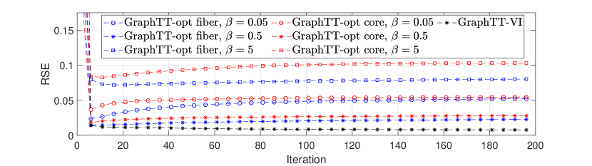
(a) w.r.t. different $\beta$, with initail ranks set as $10$

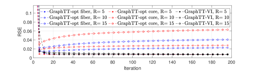
(b) w.r.t. different initial ranks, with $\beta_{0}$ set as $0.5$

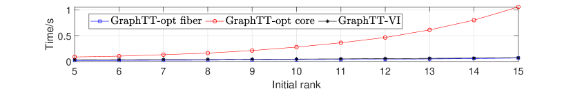
(c) Time cost for each iteration

Figure 3: Convergence of the proposed methods, under $10\text{dB}$ noise and $90\%$ missing rate.

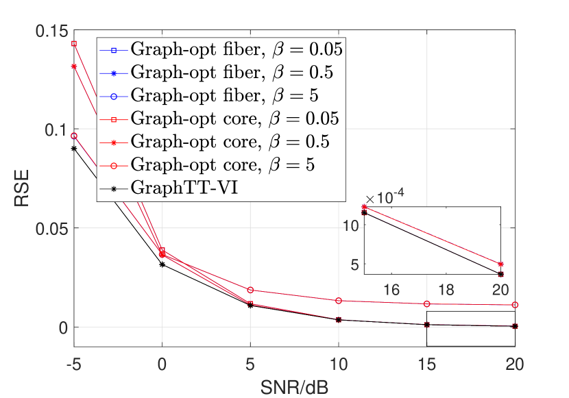
(a) w.r.t SNR, with missing rate set as $80\%$

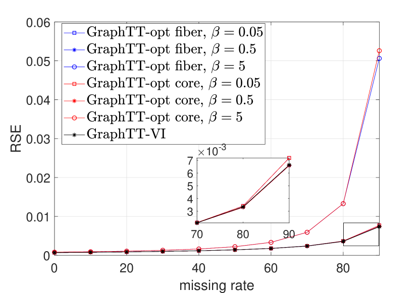
(b) w.r.t missing rate, with SNR set as $10$dB

Figure 4: Performance of the proposed methods, the initial ranks are set as the true ranks, and $\beta$ is set as $0.05$.

Fig. 3 shows the convergence performance and time cost of the compared algorithm under $10$dB SNR and $90\%$ missing rate. In Fig. 3(a) and Fig. 3(b), the effects of the regularization parameter $\beta_{0}$ (with $R=10$) and the initial ranks (with $\beta_{0}=0.5$) are tested. As can be seen, under all settings, the GraphTT-opt with fiber update and with core update both converge. However, careless choice of parameters would lead to a slower convergence, especially for the core update, e.g., $R=15$ in Fig. 3(b), which is set far away from the true rank $R=5$ and leads to bigger problem size.

It is also observed that with different regularization parameters and initial ranks, the performance of GraphTT-opt changes a lot, no matter with core update or fiber update. For example, as can be seen in Fig. 3(a), the performance of GraphTT-opt becomes better as $\beta_{0}$ goes from $0.05$ to $0.5$, but becomes worse when $\beta_{0}=5$. That is because with $\beta_{0}=0.05$, the graph information is not fully used, while with $\beta_{0}=5$, the objective function puts too much weight on the graph regularized terms compared the reconstruction error. On the other hand, Fig. 3(b) shows that even with the best regularization parameter setting in Fig. 3(a) (i.e., $\beta_{0}=0.5$), when the initial ranks becomes larger, the performance deteriorates, which is because with larger ranks the model tends to overfit the noise. In contrast, the proposed GraphTT-VI does not need any regularization parameters, and provides similar performance under different initialized TT ranks, which are even better than those of the optimization based methods. This shows the advantages of the Bayesian approach.

Furthermore, it can be seen in both Fig. 3(a) and Fig. 3(b) that GraphTT-opt with fiber update performs similarly with or better than that with core update under all parameters settings. In addition, under worse parameter setting, their performance distance is more obvious, e.g., $\beta_{0}=5$ in Fig. 3(a) and $R=15$ in Fig. 3(b). This is probably because that the fiber update is more flexible and can fall into regions around certain local minima which core update cannot reach.

Fig. 3(c) shows the consumed time for each iteration of the proposed algorithms. As can be seen, with larger initial TT ranks, the time cost grows. This is especially obvious for the GraphTT-opt with core update, in each iteration of which are $D$ matrix inverses and each of them is with complexity $\bm{O}(J_{d}^{3}R^{6})$, while the similar operation in the other two methods are with complexity $\bm{O}(J_{d}^{3}R^{2})$.

Fig. 4 show the performance of the proposed algorithms under different SNR and missing rates with initial ranks set as the true TT-ranks, and the detailed settings of other parameters are labeled in the figure. In all settings, GraphTT-VI obtains the best performance, and GraphTT-opt under fiber and core updates perform similarly. An interesting observation from Fig. 4(a) is that different $\beta_{0}$ lead to totally different performance under different SNRs, i.e., GraphTT-opt with $\beta_{0}=5$ performs the best under $-5\text{dB}$ but worst under $20\text{dB}$, and in contrast, with $\beta_{0}=0.05$ it performs the worst under $-5\text{dB}$ but the best under $20\text{dB}$. That is because with large noise, the graph regularization should be considered more important as the observed data are contaminated and not reliable, but with small noise, we can rely more on the observed data and lower the importance of the regularization terms.

From Fig. 4(b) it can be seen that with moderate SNR ($10\text{dB}$) and relative low missing rates, all methods perform similarly. However, as the missing rate goes higher, the effects of the choice of parameters becomes more obvious. With missing rate from $70\%$ to $90\%$, even with the TT-ranks initialized as the true ones, $\beta_{0}$ has a significant influence to the performance, e.g., $\beta_{0}=0.5$ provides the best performance, $\beta=0.05$ performs slightly worse but still close to that of $\beta_{0}=0.5$, and $\beta=5$ leads to unmistakably worse performance. This phenomenon is similar to that in Fig. 3(a), and so is the reason.

5.2 RGB images completion

Next we will test the performance of the proposed methods on real-world data. Noisy and incomplete images/videos with different missing patterns will be tested. Without loss of generality, all tested data are normalized such that their entries valued from $0$ to $1$. The results of the following state-of-the-art methods are also presented as comparison, with the parameters fine-tuned to their best performance.

• Simple low-rank tensor completion via TT (SiLRTC-TT) [11], which adopts the TT nuclear norm as a regularization for the TT completion;

• Tensor completion by parallel matrix factorization via TT (TMAC-TT) [11], which minimizes the reconstruction error using parallel matrix factorization;

• Tensor train completion with total variation regularizations (TTC-TV) [17], which adopts the total variation as the regularization for the TT completion;

• Probabilistic tensor train completion (PTTC) [14], which uses the Gaussian-Gamma sparsity promoting prior for the traditional TT format and solves it using variational inference. An improved folding strategy is also introduced by duplicating the folding edges.

• Tensor ring completion based on the variational Bayesian frame work (TR-VBI) [15], which builds a probabilistic model from the Gaussian-Gamma prior for the tensor ring completion and learning througth VI.

• Sparse tensor train optimization (STTO) [9], which minimizes the square error between the completed TT tensor and the observed tensor by considering only the observed entries;

• Fully Bayesian Canonical Polyadic Decomposition (FBCP) [37], which builds a probabilistic model for tensor CPD and learns it through VI methods.

• Fast low rank tensor completion (FaLRTC) [38], which adopts the tensor trace norm as the regularization for tensor completion;

For SiLRTC-TT, TMAC-TT, TTC-TV, PTTC, TR-VBI and STTO, tensor folding is performed before TT completion. The way a tensor is folded follows that in the original work. For the detailed folding strategy and parameter settings, please see the supplemental materials.

The performance of these methods is evaluated by the peak signal-to-noise ratio (PSNR) which is defined as

$$\text{PSNR}=20\log_{10}\max(\bm{\mathcal{X}})-20\log_{10}(\text{MSE}),$$ (37)

where $\max(\bm{\mathcal{X}})$ is the maximum value of the original data tensor $\bm{\mathcal{X}}$, and MSE denotes the mean square error between the completed and original images. The structural similarity index measure (SSIM) [39] is also tested, which takes more image information like luminance masking and contrast masking terms.

In this subsection, 13 RGB images with size $256\times 256\times 3$ are tested.

TABLE IV: Performance of image completion with 90% random missing entries without noise.

	SiLRTC-TT		TMAC-TT		TTC-TV		PTTC		TR-VBI		STTO		FBCP		FaLRTC		GraphTT-opt		GraphTT-VI
	PSNR	SSIM	PSNR	SSIM	PSNR	SSIM	PSNR	SSIM	PSNR	SSIM	PSNR	SSIM	PSNR	SSIM	PSNR	SSIM	PSNR	SSIM	PSNR	SSIM
airplane	19.57	0.593	21.26	0.688	20.65	0.591	22.44	0.709	21.56	0.547	20.67	0.533	19.53	0.448	18.97	0.496	22.25	0.660	23.28	0.717
baboon	19.11	0.375	19.15	0.419	20.19	0.413	20.26	0.389	19.95	0.308	19.45	0.370	18.46	0.270	18.51	0.348	19.61	0.446	20.86	0.381
barbara	20.31	0.547	22.62	0.679	20.87	0.538	23.41	0.699	22.55	0.581	22.12	0.590	19.08	0.416	18.95	0.466	24.38	0.722	24.10	0.690
couple	23.20	0.625	21.54	0.564	24.93	0.660	26.33	0.745	25.34	0.634	25.37	0.665	24.05	0.560	23.28	0.615	28.16	0.837	27.71	0.781
facade	19.34	0.424	22.10	0.654	22.04	0.620	22.25	0.636	25.33	0.775	20.81	0.560	25.56	0.799	24.74	0.788	26.10	0.828	27.16	0.839
goldhill	20.74	0.477	23.07	0.619	21.65	0.521	23.55	0.615	22.75	0.519	22.04	0.535	20.46	0.427	20.43	0.481	24.35	0.675	24.50	0.644
house	21.18	0.653	23.16	0.712	22.72	0.642	26.10	0.748	24.64	0.634	22.86	0.608	20.99	0.515	20.78	0.574	25.66	0.716	26.27	0.769
jellybeens	21.94	0.801	23.34	0.843	23.65	0.845	26.63	0.892	22.38	0.800	23.35	0.604	20.51	0.748	21.86	0.807	26.79	0.887	27.43	0.917
lena	21.52	0.601	24.28	0.700	21.63	0.551	25.25	0.728	23.48	0.571	23.60	0.636	20.16	0.408	19.74	0.469	25.27	0.725	25.02	0.714
peppers	19.05	0.570	21.40	0.656	19.79	0.559	22.41	0.688	21.00	0.545	20.82	0.582	17.68	0.360	17.00	0.384	23.32	0.709	22.69	0.715
sailboat	18.05	0.483	19.69	0.589	19.34	0.516	20.94	0.615	20.02	0.486	19.66	0.497	18.43	0.400	17.91	0.444	21.46	0.641	21.84	0.640
splash	21.24	0.662	23.84	0.729	22.93	0.672	25.74	0.743	22.90	0.646	23.10	0.667	21.47	0.605	21.93	0.663	26.08	0.757	26.49	0.765
tree	17.95	0.471	20.67	0.597	18.91	0.490	21.05	0.598	20.16	0.474	19.84	0.490	17.43	0.342	16.95	0.369	21.39	0.599	21.74	0.620

TABLE V: Performance of image completion with 90% random missing with noise variance 0.01.

	SiLRTC-TT		TMAC-TT		TTC-TV		PTTC		TR-VBI		STTO		FBCP		FaLRTC		GraphTT-opt		GraphTT-VI
	PSNR	SSIM	PSNR	SSIM	PSNR	SSIM	PSNR	SSIM	PSNR	SSIM	PSNR	SSIM	PSNR	SSIM	PSNR	SSIM	PSNR	SSIM	PSNR	SSIM
airplane	17.98	0.418	18.70	0.394	19.32	0.448	20.54	0.535	19.82	0.458	18.62	0.353	18.21	0.305	17.09	0.322	20.73	0.482	21.29	0.602
baboon	18.00	0.312	11.85	0.150	19.05	0.349	19.53	0.324	19.36	0.280	18.10	0.298	17.92	0.237	17.28	0.281	19.39	0.330	20.21	0.332
barbara	18.43	0.399	13.92	0.221	19.82	0.458	20.62	0.516	20.06	0.431	19.36	0.392	17.80	0.313	17.10	0.329	21.80	0.542	22.05	0.587
couple	21.24	0.431	15.95	0.125	22.77	0.465	22.91	0.477	22.65	0.478	21.28	0.343	21.82	0.360	20.75	0.378	23.51	0.523	24.61	0.572
facade	18.11	0.339	14.48	0.280	20.49	0.538	20.05	0.471	22.52	0.614	18.80	0.436	22.75	0.668	20.90	0.626	22.27	0.661	24.28	0.717
goldhill	18.98	0.360	13.34	0.172	20.31	0.431	21.31	0.458	20.53	0.377	20.10	0.387	19.11	0.307	18.32	0.338	21.98	0.485	22.67	0.523
house	19.19	0.452	18.14	0.287	20.80	0.473	22.30	0.527	20.87	0.494	20.04	0.377	19.20	0.339	18.25	0.345	22.90	0.515	23.73	0.634
jellybeens	19.46	0.511	20.38	0.479	21.14	0.535	22.61	0.673	22.42	0.692	19.88	0.426	19.60	0.414	18.71	0.398	22.16	0.480	23.95	0.782
lena	19.46	0.426	18.58	0.342	20.23	0.430	22.15	0.551	21.16	0.469	20.24	0.430	18.66	0.303	17.73	0.321	22.43	0.538	22.90	0.611
peppers	17.25	0.403	13.10	0.171	18.65	0.457	19.83	0.530	18.86	0.434	18.52	0.417	16.47	0.280	15.49	0.275	20.65	0.540	20.80	0.619
sailboat	16.74	0.360	13.48	0.224	18.44	0.437	19.03	0.467	18.62	0.400	18.12	0.378	17.26	0.307	16.49	0.330	19.81	0.487	20.46	0.546
splash	18.97	0.460	16.31	0.207	21.19	0.514	22.00	0.533	21.73	0.585	20.39	0.428	20.25	0.410	19.14	0.425	22.81	0.566	23.57	0.663
tree	16.66	0.359	14.87	0.276	18.12	0.425	19.03	0.445	17.74	0.332	18.44	0.407	16.50	0.258	15.70	0.279	20.00	0.487	20.38	0.528

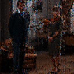
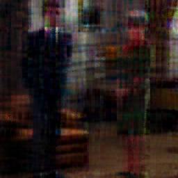
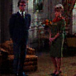
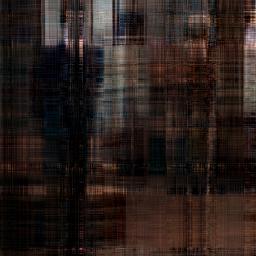
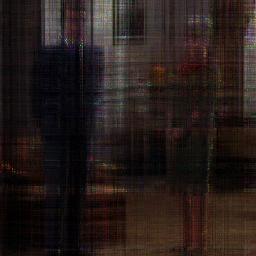
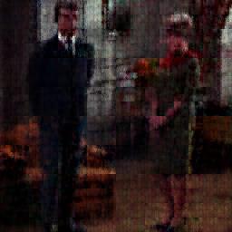
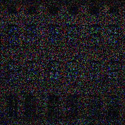
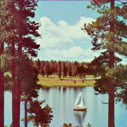
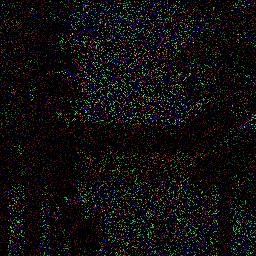
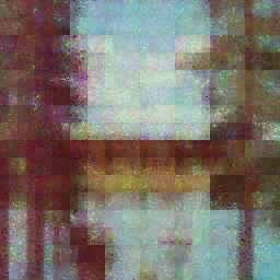
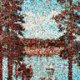
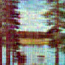
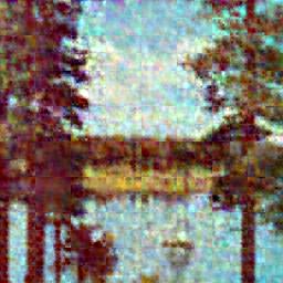
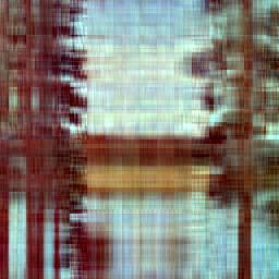
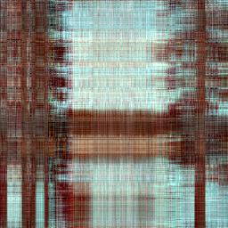
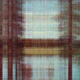
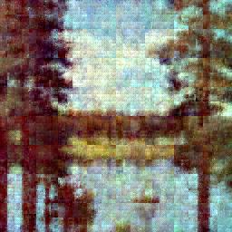
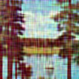
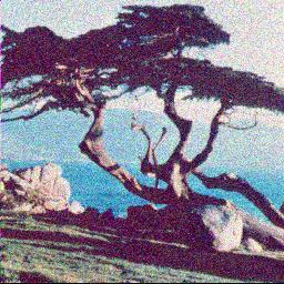
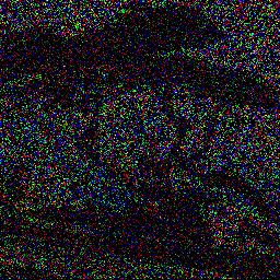
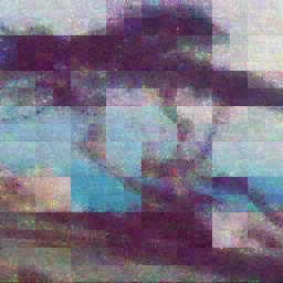
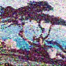
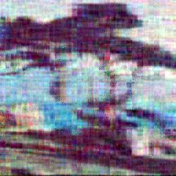
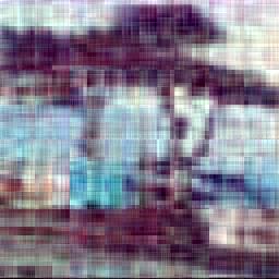
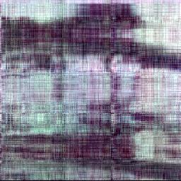
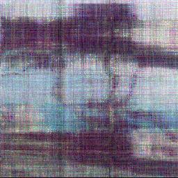
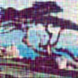
Figure 5: Visual effects of the image completion experiments, from top to bottom: recovered ’couple’ and ’facade’ images under $90\%$ missing rate and no noise, recovered ’sailboat’ and ’tree’ images under $90\%$ missing rate and Gaussian noise with mean $0$ and variance $0.01$; from left to right: original images, observed images, recovered images by SiLRTC-TT, TMAC-TT, TTC-TV, PTTC, TR-VBI, STTO, FBCP, FaLRTC, GraphTT-opt, GraphTT-VI, respectively.

5.2.1 Random missing

Firstly, images with 90 percent random missing entries are tested. Two cases are considered, which are without noise and under Gaussian noise with mean $0$ and variance $0.01$. Some original and observed images can be seen in the left two columns in Fig. 5. For the proposed algorithms, the Laplacian is generated as (8). The first two weighting matrix are with elements $\bm{W}_{i,j}^{(d)}=\text{exp}(|i-j|^{2})$, and the third one is set as an identity matrix. The initial ranks are set as $[1,64,3,1]$ for both GraphTT-opt and GraphTT-VI. For GraphTT-opt, $\beta_{0}$ is set as $2$ for the clean data and $100$ for the noisy data.

The PSNR and SSIM of the recovered images without noise are listed in Table IV. As can be seen, the two proposed algorithms GraphTT-opt and GraphTT-VI achieve the top two performances most of the time. In general, the two proposed algorithms perform similarly, and GraphTT-VI achieves an average $0.32\text{dB}$ higher PSNR but $0.001$ lower SSIM than GraphTT-opt. In comparison, GraphTT-VI achieves an average $0.98$ higher PSNR and $0.030$ higher SSIM than PTTC, which is the third best. For the ’couple’ and ’facade’ image, GraphTT-VI even achieves $1.38/1.60\text{dB}$ higher PSNR and $0.037/0.040$ higher SSIM than the third best PTTC and FBCP, respectively. The superior performance of the proposed algorithms on these two figures can also be visualized in the top two rows of Fig. 5.

TABLE VI: Performance of image completion under character mask with noise variance 0.01.

	SiLRTC-TT		TMAC-TT		TTC-TV		PTTC		TR-VBI		STTO		FBCP		FaLRTC		GraphTT-opt		GraphTT-VI
	PSNR	SSIM	PSNR	SSIM	PSNR	SSIM	PSNR	SSIM	PSNR	SSIM	PSNR	SSIM	PSNR	SSIM	PSNR	SSIM	PSNR	SSIM	PSNR	SSIM
airplane	19.50	0.473	19.37	0.470	19.48	0.471	25.43	0.722	24.36	0.605	19.31	0.459	24.41	0.613	19.41	0.465	25.22	0.674	26.13	0.728
baboon	20.11	0.636	19.92	0.630	20.11	0.635	22.49	0.591	22.26	0.580	19.92	0.622	22.42	0.607	20.04	0.631	23.00	0.637	23.27	0.632
barbara	20.08	0.540	19.83	0.531	19.94	0.532	25.96	0.731	24.77	0.663	19.87	0.526	24.64	0.667	19.97	0.533	26.35	0.737	26.41	0.744
couple	21.44	0.427	21.48	0.430	21.45	0.427	26.68	0.644	26.95	0.641	21.41	0.426	26.49	0.612	21.45	0.427	27.83	0.720	27.89	0.705
facade	20.09	0.679	19.83	0.664	20.30	0.696	25.22	0.787	26.57	0.820	19.92	0.666	27.36	0.850	20.38	0.705	27.19	0.859	28.36	0.873
goldhill	20.03	0.559	19.89	0.553	19.97	0.554	25.37	0.707	24.81	0.665	19.96	0.552	24.76	0.667	19.97	0.556	26.24	0.742	26.34	0.735
house	20.07	0.408	19.91	0.399	20.05	0.406	27.50	0.727	26.21	0.622	19.94	0.395	25.81	0.620	20.02	0.406	27.20	0.677	28.11	0.753
jellybeens	19.06	0.328	18.90	0.324	19.10	0.333	28.09	0.798	27.40	0.780	18.91	0.315	25.97	0.629	19.04	0.327	26.54	0.641	27.41	0.707
lena	20.42	0.491	20.18	0.479	20.27	0.480	26.78	0.733	24.95	0.607	20.24	0.482	24.98	0.620	20.26	0.481	26.67	0.719	27.12	0.742
peppers	19.66	0.488	19.31	0.473	19.46	0.480	25.53	0.746	24.09	0.660	19.46	0.477	23.44	0.635	19.45	0.477	25.60	0.730	25.70	0.761
sailboat	19.83	0.557	19.63	0.547	19.78	0.553	24.22	0.711	23.54	0.645	19.75	0.550	23.64	0.661	19.86	0.557	24.65	0.722	25.02	0.740
splash	20.50	0.419	20.33	0.412	20.50	0.421	27.17	0.705	27.10	0.687	20.46	0.418	26.42	0.653	20.52	0.421	27.12	0.706	28.25	0.764
tree	19.91	0.568	19.55	0.557	19.70	0.560	24.54	0.705	23.54	0.639	19.78	0.557	23.31	0.636	19.76	0.560	24.64	0.704	25.03	0.725

TABLE VII: Average runtime/s of all the compared methods in experiments on RGB images.

	SiLRTC-TT	TMAC-TT	TTC-TV	PTTC	TR-VBI	STTO	FBCP	FaLRTC	GraphTT-opt	GraphTT-VI
Random missing, clean	32.62	63.74	27.97	641.22	148.40	315.65	24.87	22.45	43.30	101.40
Random missing, noisy	36.98	69.65	25.70	466.15	99.82	313.07	25.39	23.55	25.77	104.98
Character missing, noisy	14.26	1.37	32.13	1405.28	717.64	311.47	46.51	2.86	13.00	123.10

(a) Original

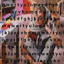
(b) Observed

(c) Recovered by SiLRTC-TT

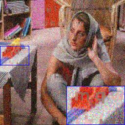
(d) Recovered by TMAC-TT

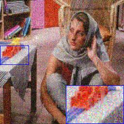
(e) Recovered by TTC-TV

(f) Recovered by PTTC

(g) Recovered by TR-VBI

(h) Recovered by STTO

(i) Recovered by FBCP

(j) Recovered by FaLRTC

(k) Recovered by GraphTT-opt

(l) Recovered by GraphTT-VI

Figure 6: Recovered ’barbara’ images with character missing and noise variance $0.01$.

When there is noise, the performance of all algorithms deteriorate as shown in Talbe V. However, GraphTT-VI still keeps the best performance, achieving an average $0.80\text{dB}$ higher PSNR and $0.083$ higher SSIM than the overall second best, GraphTT-opt. From the bottom two rows of Fig. 5, it can be seen that among all the tested methods, only TMAC-TT, PTTC, GraphTT-opt and GraphTT-VI recover relatively clear ’sailboat’ and ’tree’ images. In addition, GraphTT-opt and GraphTT-VI are less affected by noise than TMAC-TT and PTTC. However, from the visual effects it is also noticed that even though the proposed algorithms achieve the best PSNR and SSIM, they tend to oversmooth the images under bad conditions like high missing rate and heavy noise. That is due to the effect of the graph regularization, which plays a more important role than reconstruction error under these conditions.

The average runtimes of all the compared methods on the $13$ images is listed in the first two rows in Table VII. As can be seen, the proposed GraphTT-opt and GraphTT-VI achieve the overall best performance mentioned above at the cost of a moderate runtime. Specifically, GraphTT-VI takes twice to fifth times longer than GraphTT-opt, mainly due to the more complicated expectations in the VI update. However, it should be recognized that GraphTT-VI does not require any parameter tuning, which is practically helpful since there would not be any ground-truth images for computing the PSNR or SSIM. Even if a tuning strategy could be adopted without the ground-truth, the exhaustive tuning may eventually end up with a longer runtime.

5.2.2 Character missing patterns

Character missing patterns are considered in this subsection. Every image is added with Gaussian noise with zero mean and variance $0.01$. An example of the observed image is shown as Fig. 6(b). The Laplacian matrices and initial ranks are set the same as in the previous experiments for both GraphTT-VI and GraphTT-opt, and $\beta_{0}$ is set as $100$ for GraphTT-opt, the same as that in the noisy random missing case.

The performance of the compared methods are presented in Table. VI. GraphTT-VI achieves the best performance for all images except for the SSIM in ’baboon’, and GraphTT-opt and PTTC achieve the second best for most of the images. The visual effects of the recovered images from the corrupted ’barbara’ image are shown in Fig. 6. From the bottom right of each figure it can be seen that the proposed methods perform the best in terms of removing the character missing patterns, with gray character marks clearly seen in other optimization based methods. It also worth noticing that except GraphTT-opt, other methods that remove characters well are all based on Bayesian modeling, i.e., PTTC, TR-VBI and FBCP, which again manifests the advantage of Bayesian modeling in tensor completion tasks.

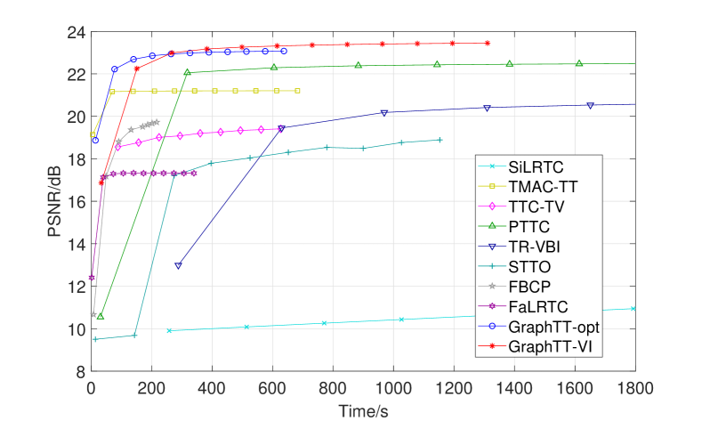
Figure 7: Performance of completion on YaleFace Dataset under 90% random entry missing and 20% random pose missing with noise variance 0.01.

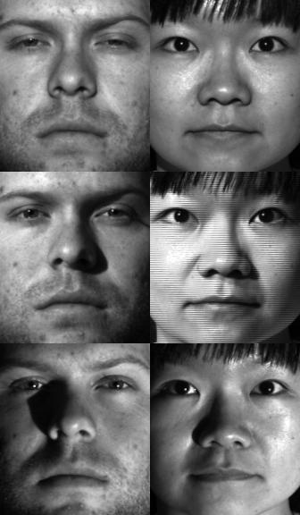
(a) Original

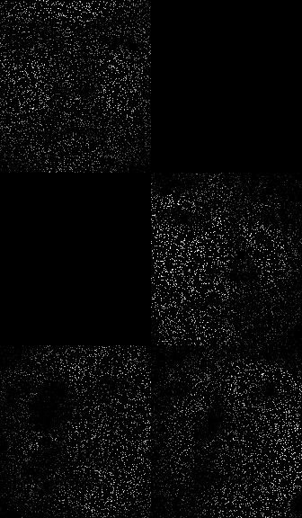
(b) Observed

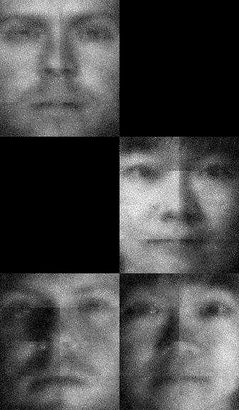
(c) SiLRTC-TT

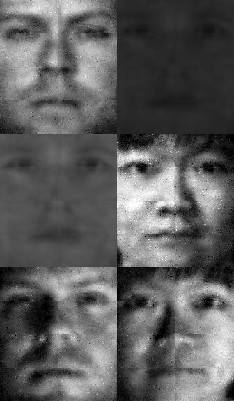
(d) TMAC-TT

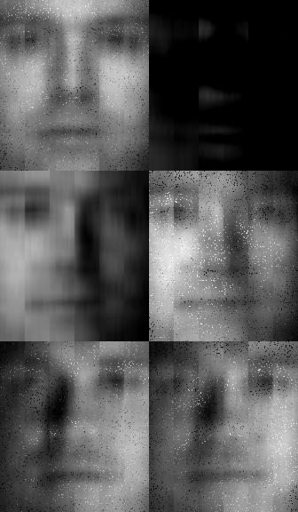
(e) TTC-TV

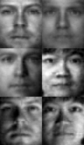
(f) PTTC

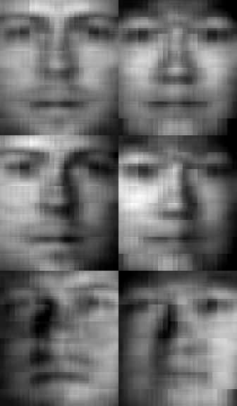
(g) TR-VBI

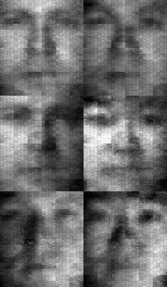
(h) STTO

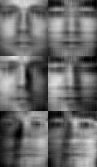
(i) FBCP

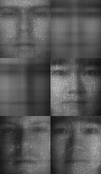
(j) FaLRTC

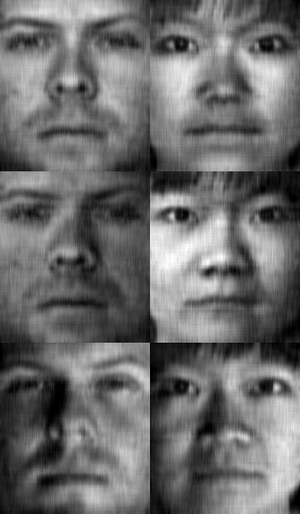
(k) GraphTT-opt

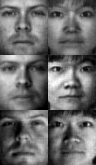
(l) GraphTT-VI

Figure 8: Recovered face data under 90% random element missing rate, 20% random pose missing rate and 0.01 noise variance.

The average runtimes of the compared algorithms are presented in the third row of Table VII. As can be seen, the proposed methods cost moderate times among all competing algorithms. Specifically, SiLRTC-TT, TMAC-TT, FaLRTC and GraphTT-opt take obviously less time than that in the random missing cases, mainly because they converge faster due to more observed entries.

5.3 YaleFace dataset

In this subsection, the YaleFace dataset, which contains gray images of 38 people under 64 illumination conditions, each with size $192\times 168$, is adopted. Without loss of generality, images of 10 people are chosen, resulting in a data tensor with size 192×168×64×10. $90\%$ elements are randomly removed, and Gaussian noise with mean $0$ and variance $0.01$ is added to the dataset. Apart from that, $20\%$ of poses are furhter randomly removed. For the proposed algorithm, the Laplacian as in (8) is adopted. For the first $3$ TT cores, the weighting matrix is with element $\bm{W}_{i,j}=\text{exp}(|i-j|^{2})$, and for the last TT core, the weighting matrix is set as an identity matrix. The reason why such a Laplacian matrix is adopted for the $3$rd TT core is that the pose image of the same person will not change much, even under different illuminations. The initial ranks for both the proposed algorithms are $[1,32,32,10,1]$, and $\beta_{0}$ is set as $100$ for GraphTT-opt. The visual effects of the $7$th, $16$th and $48$th poses of the $1$st and $5$th person are shown in Fig. 8(b), in which the second pose of the man and the first pose of the woman are totally missing.

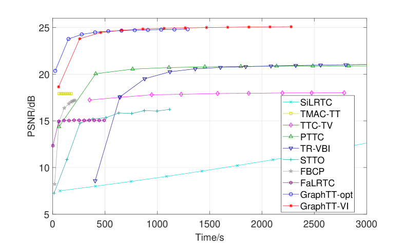
Figure 9: Performance of video completion under 90% random entry missing and 20% random pose missing with noise variance 0.01.

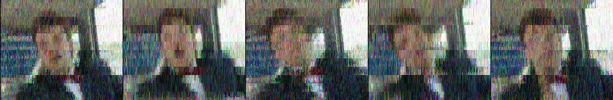
Figure 10: Recovered ’carphone’ video under 90% random element missing, 20% random frame missing and noise variance 0.01. From top to bottom (left): the original images, the observed images, recovered images by SiLRTC-TT, TMAC-TT, TTC-TV and PTTC; (right): recovered images by TR-VBI, STTO, FBCP, FaLRTC, GraphTT-opt, and GraphTT-VI, respectively.

The PSNR of various methods w.r.t. runtime is presented in Fig. 7. As can be seen, since about $250s$, GraphTT-VI and GraphTT-opt keep the highest and second highest PSNR. Their good performance can also be observed from the visual effects in Fig. 8, which shows the recovered face images after the algorithms converging. From Fig. 8 it can be seen that only TMAC-TT, PTTR and the proposed methods recovered recognizable images. For the pose images that are totally missing, TMAC-TT fails to recover them. For PTTR, even though it tries to recover the missing pose and achieves the third highest PSNR, it wrongly borrows information from other people, leading to its top right image look like a man. In particular, the block effects are obviously seen for the methods combined with tensor folding, as shown in Fig. 8(c)-8(h). Additionally, due to the heavy memory consumption caused by the update on a whole TT core, the initial ranks for TTC-TV and TR-VBI are bounded by $10$, which is the highest value possible for them to run without exceeding the memory limitation (32GB). However, the ranks are too small to recover the details of the data, leading to blurred face images shown in Fig. 8(e) and 8(g).

5.4 Video Completion

In this subsection, we assess the performance of the proposed methods on video completion. A color video with size $144\times 176\times 3\times 382$ is tested with $90\%$ elements randomly missed, plus $20\%$ frames randomly missed, and Gaussian noise with mean $0$ and variance $0.01$ added. The parameter setting follows those in the YaleFace experiment, except that the $3$rd Laplacian matrix is set as an identity matrix while the $4$th is set as one that measures similarity between pixels. The reason is that there is no particular relations between RGB pixels, but for nearby time frames, they tend to be similar with each other. The $44$th, $64$th, $84$th, $104$th and $124$th frames of the video are presented in the second line of Fig. 10, among which the $64$th and $104$th frames are totally missing under observation.

The performance of the compared methods w.r.t. runtime is shown in Fig. 9, with the visual effects of the corresponding recovered frames after algorithms converging shown in Fig. 10. As can be seen from Fig. 9, graphTT-VI and graphTT-opt keep the highest two PSNR’s all the time, and achieve about $4$dB higher PSNR than the third best after convergence. From Fig. 10, it can be seen that the proposed methods recover videos with recognizable faces and expressions, while most other compared methods cannot. Though PTTC also generate recognizable faces for normal frames, they cannot handle cases when a whole frame is missing. On the other hand, though TMAC-TT and TR-VBI provides estimations of the missing frames, the recovered frames are hard to recognize, as those recovered by TMAC-TT are highly corrupted with noise, while those recovered by TR-VBI are blurry.

6 Conclusion

In this paper, a graph regularized TT completion method was proposed for visual data completion without the need of folding a tensor. To overcome the high computational burden introduced by the graph regularization without tensor folding, tensor core fibers were updated as the basic blocks under the BCD framework. Based on that, a probabilistic graph regularized TT model, which has the ability to automatically learn the TT ranks and the regularization parameters, was further proposed. Experiments on synthetic data showed that the proposed optimization based method with fiber update performs similarly to core update, but is much more computational efficient. Further experiments on image and video data showed the superiority of the proposed algorithms, especially for GraphTT-VI, which achieves the overall best performance compared to other state-of-the-art methods under different settings without the need to finetune parameters.

This paper partially answered the question of to fold or not to fold in TT completion: if the graph information is provided and put along each mode of the TT-format tensor, then in general not to fold would give better performance. However, a further question might be if the graph information could be provided among every two elements like that in (9) and the heavy computational burden could be overcome, then would not folding a tensor still a better option? This is a good topic for future work.

Appendix A Derivation of (15)

Since $\|\bm{A}+\bm{B}\|_{F}^{2}=\|\bm{A}\|_{F}^{2}+\|\bm{B}\|_{F}^{2}+2\text{tr}(\bm{A}^{T}\bm{B})$, (14) can be re-written as

$$\min_{{\bm{G}_{(3)}^{(d)}}_{:,p}}\bigg{\|}\bm{O}_{(d)}\ast\big{(}{\bm{G}_{(3)}^{(d)}}_{:,p}\Big{[}\bm{G}_{(1)}^{(>d)}\otimes\bm{G}_{(d)}^{(<d)}\Big{]}_{p,:}\big{)}\bigg{\|}_{F}^{2}$$

$$+\beta_{d}{\bm{G}_{(3)}^{(d)}}_{:,p}^{T}\bm{L}^{(d)}{\bm{G}_{(3)}^{(d)}}_{:,p}-2\text{tr}\bigg{(}\bm{\Xi}^{T}\Big{(}\bm{O}_{(d)}\ast({\bm{G}_{(3)}^{(d)}}_{:,p}$$

$$\times\Big{[}\bm{G}_{(1)}^{(>d)}\otimes\bm{G}_{(d)}^{(<d)}\Big{]}_{p,:})\Big{)}\bigg{)}.$$ (38)

It is clearly that (38) is quadratic with respect to each TT core fiber ${\bm{G}_{(3)}^{(d)}}_{:,p}$. In order to obtain the solution of (38), we put the objective function of (38) into a standard form ${\bm{G}_{(3)}^{(d)}}_{:,p}^{T}\bm{\Upsilon}{\bm{G}_{(3)}^{(d)}}_{:,p}+\bm{\mu}^{T}{\bm{G}_{(3)}^{(d)}}_{:,p}$. For $\bm{\Upsilon}$, it comes from the Frobenius norm and the graph regularization term in (38), the latter of which is obvious. Since

$$\bigg{\|}\bm{O}\ast(\bm{a}\bm{b}^{T})\bigg{\|}_{F}^{2} =\sum_{i=1}\sum_{j=1}\bm{O}_{ij}\bm{a}_{i}^{2}\bm{b}_{j}^{2}=\sum_{i}\bm{a}_{i}^{2}(\sum_{j}\bm{O}_{ij}\bm{b}_{j}^{2})$$

$$=\sum_{i}\bm{a}_{i}^{2}\bm{O}_{i,:}(\bm{b}\ast\bm{b})=\bm{a}^{T}\text{diag}\Big{(}\bm{O}(\bm{b}\ast\bm{b})\Big{)}\bm{a},$$

in which $\bm{O}$ is a boolean matrix, the Frobenius norm in (38) can be written as

$${\bm{G}_{(3)}^{(d)}}_{:,p}^{T}\text{diag}\bigg{(}\bm{O}_{(d)}(\Big{[}\bm{G}_{(1)}^{(>d)}\otimes\bm{G}_{(d)}^{(<d)}\Big{]}_{p,:}^{T}$$

$$\quad\ast\Big{[}\bm{G}_{(1)}^{(>d)}\otimes\bm{G}_{(d)}^{(<d)}\Big{]}_{p,:}^{T})\bigg{)}{\bm{G}_{(3)}^{(d)}}_{:,p}.$$ (39)

For the coefficient $\bm{\mu}$, since

$$\text{tr}\bigg{(}\bm{Y}^{T}\Big{(}\bm{O}\ast(\bm{a}\bm{b}^{T})\Big{)}\bigg{)}=\sum_{i}\sum_{j}\bm{O}_{ij}\bm{Y}_{ij}\bm{a}_{i}\bm{b}_{j}$$

$$=\sum_{i}\bm{a}_{i}(\sum_{j}\bm{O}_{ij}\bm{Y}_{ij}\bm{b}_{j})=\Big{(}(\bm{O}\ast\bm{Y})\bm{b}\Big{)}^{T}\bm{a},$$

the trace term in (38) can be written as

$$-2\bigg{(}\Big{(}\bm{O}_{(d)}\ast\bm{\Xi}\Big{)}\Big{[}\bm{G}_{(1)}^{(>d)}\otimes\bm{G}_{(d)}^{(<d)}\Big{]}_{p,:}^{T}\bigg{)}{\bm{G}_{(3)}^{(d)}}_{:,p}.$$ (40)

Therefore, (38) can be formulated as

$$\min_{\bm{\mathcal{G}}_{r_{d},r_{d+1},:}^{(d)}}{\bm{G}_{(3)}^{(d)}}_{:,p}^{T}\bm{\Upsilon}{\bm{G}_{(3)}^{(d)}}_{:,p}-2\bm{\mu}^{T}{\bm{G}_{(3)}^{(d)}}_{:,p},$$ (41)

with

$$\bm{\Upsilon} =\text{diag}\bigg{(}\bm{O}_{(d)}(\Big{[}\bm{G}_{(1)}^{(>d)}\otimes\bm{G}_{(d)}^{(<d)}\Big{]}_{p,:}^{T}$$

$$\ast\Big{[}\bm{G}_{(1)}^{(>d)}\otimes\bm{G}_{(d)}^{(<d)}\Big{]}_{p,:}^{T})\bigg{)}+\beta_{d}\bm{L}^{(d)},$$ (42)

$$\bm{\mu} =\Big{(}\bm{O}_{(d)}\ast\bm{\Xi}\Big{)}\Big{[}\bm{G}_{(1)}^{(>d)}\otimes\bm{G}_{(d)}^{(<d)}\Big{]}_{p,:}^{T},$$ (43)

and the solution of (41) is given by ${\bm{G}_{(3)}^{(d)}}_{:,p}={\bm{\Upsilon}}^{-1}\bm{\mu}$.

Appendix B Derivation of VI TT completion with graph regularization

Firstly, based on the proposed probabilistic model (19)-(23), the logarithm of the joint distribution of the observed tensor and all the variables is derived as

$$\ln{\left({p(\bm{\mathcal{Y}},\bm{\Theta})}\right)}$$

$$=\frac{|\Omega|}{2}\ln{\tau}-\frac{\tau}{2}\left\|\bm{\mathcal{O}}\ast\big{(}\bm{\mathcal{Y}}-\ll\bm{\mathcal{G}}^{(1)},\bm{\mathcal{G}}^{(2)},\ldots,\bm{\mathcal{G}}^{(D)}\gg\big{)}\right\|_{F}^{2}$$

$$-\frac{1}{2}\sum_{d=1}^{D}\sum_{k}^{S_{d}}\sum_{\ell}^{S_{d+1}}\Big{(}J_{d}\ln(\bm{z}_{k}^{(d)}\bm{z}_{\ell}^{(d+1)})+\frac{{{\bm{\mathcal{G}}_{k,\ell,:}^{(d)}}}^{T}\bm{L}^{(d)}{{\bm{\mathcal{G}}_{k,\ell,:}^{(d)}}}}{\bm{z}_{k}^{(d)}\bm{z}_{\ell}^{(d+1)}}\Big{)}$$

$$+\sum_{d=2}^{D}\sum_{k=1}^{S_{d}}\Big{(}\big{(}\bm{\lambda}_{k}^{(d)}-1\big{)}{\ln{\bm{z}_{k}^{(d)}}}-\frac{1}{2}(\bm{a}_{k}^{(d)}\bm{z}_{k}^{(d)}+\bm{b}_{k}^{(d)}\frac{1}{\bm{z}_{k}^{(d)}})$$

$$+\frac{\bm{\lambda_{k}^{(d)}}}{2}\ln\bm{a}_{k}^{(d)}+(\bm{c}_{d}-1)\ln\bm{a}_{k}^{(d)}-\bm{f}_{d}\bm{a}_{k}^{(d)}\Big{)}+\left(a_{\tau}-1\right)\ln{\tau}$$

$$-b_{\tau}\tau+\text{const}.$$ (44)

To make the equations of VI update be expressed using notations in deterministic optimization algorithm in Section 3, we notice that $\bm{\mathcal{G}}_{k,\ell,:}^{(d)}$ with $k$ from $1$ to $S_{d}$ and $\ell$ from $1$ to $S_{d+1}$ is equivalent to ${\bm{G}_{(3)}^{(d)}}_{:,p}$ for $p$ from $1$ to $S_{d}S_{d+1}$, under the bijection $p=(\ell_{p}-1)S_{d}+k_{p}$.

$$\ln{q({\bm{G}_{(3)}^{(d)}}_{:,p})} =-\mathbb{E}_{\bm{\Theta}\setminus{\bm{G}_{(3)}^{(d)}}_{:,p}}\bigg{\llbracket}\frac{\tau}{2}\left\|\bm{\mathcal{O}}\ast\big{(}\bm{\mathcal{Y}}-\ll\bm{\mathcal{G}}^{(1)},\bm{\mathcal{G}}^{(2)},\ldots,\bm{\mathcal{G}}^{(D)}\gg\big{)}\right\|_{F}^{2}+\frac{{\bm{G}_{(3)}^{(d)}}_{:,p}^{T}\bm{L}^{(d)}{\bm{G}_{(3)}^{(d)}}_{:,p}}{\bm{z}_{k_{p}}^{(d)}\bm{z}_{\ell_{p}}^{(d+1)}}\bigg{\rrbracket}+\text{const}$$

$$=-\frac{1}{2}{\bm{G}_{(3)}^{(d)}}_{:,p}^{T}\Bigg{(}\mathbb{E}{\big{\llbracket}\tau\big{\rrbracket}}\text{diag}\bigg{(}\bm{O}_{(d)}\mathbb{E}\bigg{\llbracket}\Big{[}\bm{G}_{(1)}^{(>d)}\otimes\bm{G}_{(d)}^{(<d)}\Big{]}_{p,:}^{T}\ast\Big{[}\bm{G}_{(1)}^{(>d)}\otimes\bm{G}_{(d)}^{(<d)}\Big{]}_{p,:}^{T}\bigg{\rrbracket}\bigg{)}+\mathbb{E}\bigg{\llbracket}\frac{1}{\bm{z}_{k_{p}}^{(d)}\bm{z}_{\ell_{p}}^{(d+1)}}\bigg{\rrbracket}\bm{L}^{(d)}\Bigg{)}{\bm{G}_{(3)}^{(d)}}_{:,p}$$

$$+\mathbb{E}{\big{\llbracket}\tau\big{\rrbracket}}\Bigg{(}\Big{(}\bm{O}_{(d)}\ast\bm{Y}_{(d)}\Big{)}\mathbb{E}\bigg{\llbracket}\Big{[}\bm{G}_{(1)}^{(>d)}\otimes\bm{G}_{(d)}^{(<d)}\Big{]}_{p,:}^{T}\bigg{\rrbracket}$$

$$-\mathbb{E}\bigg{\llbracket}\underbrace{\bm{O}_{(d)}\ast\Big{(}\sum_{q=1,q\neq p}^{S_{d}S_{d+1}}{\bm{G}_{(3)}^{(d)}}_{:,q}\Big{[}\bm{G}_{(1)}^{(>d)}\otimes\bm{G}_{(d)}^{(<d)}\Big{]}_{q,:}\Big{)}\Big{[}\bm{G}_{(1)}^{(>d)}\otimes\bm{G}_{(d)}^{(<d)}\Big{]}_{p,:}^{T}}_{\bm{\phi}}\bigg{\rrbracket}\Bigg{)}^{T}{\bm{G}_{(3)}^{(d)}}_{:,p}+\text{const},$$ (45)

Then, according to the optimal variational distribution (25), $q({\bm{G}_{(3)}^{(d)}}_{:,p})$ is obtained by taking expectation on (44) and focusing on terms that are only related to ${\bm{G}_{(3)}^{(d)}}_{:,p}$, in which previous results (14), (38)-(40) are used. It can be seen that (45) is quadratic with respect to ${\bm{G}_{(3)}^{(d)}}_{:,p}$, and therefore it follows a Gaussian distribution with covariance matrix and mean

$$\bm{\Sigma}^{(d,p)}=\Bigg{(}\mathbb{E}\bigg{\llbracket}\frac{1}{\bm{z}_{k_{p}}^{(d)}}\bigg{\rrbracket}\mathbb{E}\bigg{\llbracket}\frac{1}{\bm{z}_{\ell_{p}}^{(d+1)}}\bigg{\rrbracket}\bm{L}^{(d)}+\mathbb{E}{\big{\llbracket}\tau\big{\rrbracket}}\text{diag}\bigg{(}\bm{O}_{(d)}$$

$$\times\mathbb{E}\bigg{\llbracket}\underbrace{\Big{[}\bm{G}_{(1)}^{(>d)}\otimes\bm{G}_{(d)}^{(<d)}\Big{]}_{p,:}^{T}\ast\Big{[}\bm{G}_{(1)}^{(>d)}\otimes\bm{G}_{(d)}^{(<d)}\Big{]}_{p,:}^{T}}_{\bm{\mathcal{KG}}_{p,p,:}^{(d)}}\bigg{\rrbracket}\bigg{)}\Bigg{)}^{-1},$$ (46)

$$\bm{\nu}^{(d,p)}=\mathbb{E}{\big{\llbracket}\tau\big{\rrbracket}}\bm{\Sigma}^{(d,p)}\bigg{(}\Big{(}\bm{O}_{(d)}\ast\bm{Y}_{(d)}\Big{)}\mathbb{E}\bigg{\llbracket}\Big{[}\bm{G}_{(1)}^{(>d)}\otimes\bm{G}_{(d)}^{(<d)}\Big{]}_{p,:}^{T}\bigg{\rrbracket}$$

$$-\mathbb{E}\big{\llbracket}\bm{\phi}\big{\rrbracket}\bigg{)},$$ (47)

respectively, where $\bm{\mathcal{KG}}_{q,p,:}^{(d)}\in\mathbb{R}^{J_{1}\ldots J_{d-1}J_{d+1}\ldots J_{D}}$ is defined as $\Big{[}\bm{G}_{(1)}^{(>d)}\otimes\bm{G}_{(d)}^{(<d)}\Big{]}_{q,:}^{T}\ast\Big{[}\bm{G}_{(1)}^{(>d)}\otimes\bm{G}_{(d)}^{(<d)}\Big{]}_{p,:}^{T}$ for any $q$ and $p$ from $1$ to $S_{d}S_{d+1}$. The difficulty of calculating (46) and (47) comes from the expectation of $\bm{\mathcal{KG}}_{p,p,:}^{(d)}$ and $\bm{\phi}$, in which the TT cores are heavily coupled and contains square terms. Below we will first rewriting $\bm{\phi}$, which turns out is related to $\mathbb{E}\llbracket\bm{\mathcal{KG}}_{q,p,:}^{(d)}\rrbracket$.

Since

$$\Big{[}\big{(}\bm{A}\ast(\bm{b}\bm{c}^{T})\big{)}\bm{d}\Big{]}_{i}=\bm{b}_{i}\sum_{j}\bm{A}_{ij}\bm{c}_{j}\bm{d_{j}},$$

it can be verified that $\big{(}\bm{A}\ast(\bm{b}\bm{c}^{T})\big{)}\bm{d}=\text{diag}(\bm{b})\bm{A}(\bm{c}\ast\bm{d})$. Using this result, we obtain

$$\mathbb{E}\big{\llbracket}\bm{\phi}\big{\rrbracket}=\sum_{q=1,q\neq p}^{S_{d}S_{d+1}}\text{diag}\bigg{(}\mathbb{E}\Big{\llbracket}{\bm{G}_{(3)}^{(d)}}_{:,q}\Big{\rrbracket}\bigg{)}\bm{O}_{(d)}$$

$$\times\mathbb{E}\bigg{\llbracket}\underbrace{\Big{[}\bm{G}_{(1)}^{(>d)}\otimes\bm{G}_{(d)}^{(<d)}\Big{]}_{q,:}^{T}\ast\Big{[}\bm{G}_{(1)}^{(>d)}\otimes\bm{G}_{(d)}^{(<d)}\Big{]}_{p,:}^{T}}_{\bm{\mathcal{KG}}_{q,p,:}^{(d)}}\bigg{\rrbracket}.$$ (48)

According to Definition 2 and the definition of $\bm{G}^{(<d)}$ and $\bm{G}^{(>d)}$ in Property 1,

$$\bm{\mathcal{KG}}_{q,p,i}^{(d)}=\bigg{(}\bm{\mathcal{G}}_{1,:,j_{1}}^{(1)}\ldots\bm{\mathcal{G}}_{:,m,j_{d-1}}^{(d-1)}\bm{\mathcal{G}}_{n,:,j_{d}}^{(d+1)}\ldots\bm{\mathcal{G}}_{:,1,j_{D}}^{(D)}\bigg{)}$$

$$\quad\times\bigg{(}\bm{\mathcal{G}}_{1,:,j_{1}}^{(1)}\ldots\bm{\mathcal{G}}_{:,k,j_{d-1}}^{(d-1)}\bm{\mathcal{G}}_{\ell,:,j_{d}}^{(d+1)}\ldots\bm{\mathcal{G}}_{:,1,j_{D}}^{(D)}\bigg{)}$$

$$=\Big{(}\bm{\mathcal{G}}_{1,:,j_{1}}^{(1)}\otimes\bm{\mathcal{G}}_{1,:,j_{1}}^{(1)}\Big{)}\ldots\Big{(}\bm{\mathcal{G}}_{:,m,j_{d-1}}^{(d-1)}\otimes\bm{\mathcal{G}}_{:,k,j_{d-1}}^{(d-1)}\Big{)}$$

$$\quad\times\Big{(}\bm{\mathcal{G}}_{n,:,j_{d+1}}^{(d+1)}\otimes\bm{\mathcal{G}}_{\ell,:,j_{d+1}}^{(d+1)}\Big{)}\ldots\Big{(}\bm{\mathcal{G}}_{:,1,j_{D}}^{(D)}\otimes\bm{\mathcal{G}}_{:,1,j_{D}}^{(D)}\Big{)},\$$ (49)

with bijections $i=j_{1}+\prod_{s=2,s\neq d}^{D}\Big{(}(j_{s}-1)\prod_{t=1,t\neq d}^{s-1}J_{t}\Big{)}$, $q=(n-1)R_{d}+m$ and $p=(\ell-1)S_{d}+k$. In the last line of (49), since the TT cores are separated, expectation of $\bm{\mathcal{KG}}$ can be obtained by the product of the expectations on the kronecker product of the TT core frontal slices

$$\mathbb{E}\big{\llbracket}\bm{\mathcal{G}}_{:,:,j_{t}}^{(t)}\otimes\bm{\mathcal{G}}_{:,:,j_{t}}^{(t)}\big{\rrbracket}=\mathbb{E}\big{\llbracket}\bm{\mathcal{G}}_{:,:,j_{t}}^{(t)}\big{\rrbracket}\otimes\mathbb{E}\big{\llbracket}\bm{\mathcal{G}}_{:,:,j_{t}}^{(t)}\big{\rrbracket}$$

$$+\underbrace{\mathbb{E}\Big{\llbracket}\big{(}\bm{\mathcal{G}}_{:,:,j_{t}}^{(t)}-\mathbb{E}\llbracket\bm{\mathcal{G}}_{:,:,j_{t}}^{(t)}\rrbracket\big{)}\otimes\big{(}\bm{\mathcal{G}}_{:,:,j_{t}}^{(t)}-\mathbb{E}\llbracket\bm{\mathcal{G}}_{:,:,j_{t}}^{(t)}\rrbracket\big{)}\Big{\rrbracket}}_{\bm{\mathrm{Var}}^{(t,j_{t})}},$$ (50)

where $\mathbb{E}\big{\llbracket}\bm{\mathcal{G}}_{k,\ell,j_{t}}^{(t)}\big{\rrbracket}=\bm{\nu}_{j_{t}}^{(t,(\ell-1)S_{t}+k)}$, and $\bm{\mathrm{Var}}^{(t,j_{t})}$ comes from the covariance matrix of $\bm{\mathcal{G}}_{:,:,j_{t}}^{(t)}$ but with elements permuted in another order. Since the mean-field approximation (26) assumes that different mode-$3$ fibers of $\bm{\mathcal{G}}^{(d)}$ are independent of each other, $\bm{\mathrm{Var}}^{(t,j_{t})}$ would be a very sparse matrix, in which only elements with index pairs $[\{(k-1)R_{t}+k\}_{k=1}^{R_{t}},\{(\ell-1)R_{t+1}+\ell\}_{\ell=1}^{R_{t+1}}]$ are non-zero, with value

$$\quad\bm{\mathrm{Var}}_{(k-1)S_{t}+k,(\ell-1)S_{t+1}+\ell}^{(t,j_{t})}=\bm{\Sigma}_{j_{t},j_{t}}^{(t,(\ell-1)S_{t}+k)}.$$ (51)

On the other hand, the variational distribution of $\bm{z}^{(d)}$ is obtained by taking expectations on (44) and focusing only on the terms related to $\bm{z}^{(d)}$, it is obtained that

$$\ln q(\bm{z}^{(d)})=\sum_{k=1}^{S_{d}}\ln q(\bm{z}_{k}^{(d)})+\text{const},$$

with

$$\ln q(\bm{z}_{k}^{(d)})=\bigg{(}\bm{\lambda}_{k}^{(d)}-\frac{J_{d}S_{d+1}}{2}-\frac{J_{d-1}S_{d-1}}{2}-1\bigg{)}\ln\bm{z}_{k}^{(d)}$$

$$-\frac{1}{2}\bigg{(}\mathbb{E}\llbracket\bm{a}_{k}^{(d)}\rrbracket\bigg{)}\bm{z}_{k}^{(d)}-\frac{1}{2}\bigg{(}\bm{b}_{k}^{(d)}+\sum_{\ell=1}^{S_{d-1}}\mathbb{E}\big{\llbracket}\frac{1}{\bm{z}_{\ell}^{(d-1)}}\big{\rrbracket}$$

$$\times\mathbb{E}\big{\llbracket}{\bm{\mathcal{G}}_{\ell,k,:}^{(d-1)}}^{T}\bm{L}^{(d-1)}\bm{\mathcal{G}}_{\ell,k,:}^{(d-1)}\big{\rrbracket}$$

$$+\sum_{\ell=1}^{S_{d+1}}\mathbb{E}\big{\llbracket}\frac{1}{\bm{z}_{\ell}^{(d+1)}}\big{\rrbracket}\mathbb{E}\big{\llbracket}{\bm{\mathcal{G}}_{\ell,k,:}^{(d)}}^{T}\bm{L}^{(d)}\bm{\mathcal{G}}_{\ell,k,:}^{(d)}\big{\rrbracket}\bigg{)}\frac{1}{\bm{z}_{k}^{(d)}}.$$ (52)

Notice that in (52) there are only terms linear to $\ln\bm{z}_{k}^{(d)}$, $\bm{z}_{k}^{(d)}$ and ${1}/{\bm{z}_{k}^{(d)}}$. Comparing (52) to (22), we obtain that $\bm{z}_{k}^{(d)}$ follows $\text{GIG}(\hat{\bm{a}_{k}^{(d)}},\hat{\bm{\lambda}}_{k}^{(d)},\hat{\bm{b}}_{k}^{(d)})$, with parameters

$$\hat{\bm{a}}_{k}^{(d)}=\mathbb{E}\big{\llbracket}{\bm{a}_{k}^{(d)}}\big{\rrbracket},$$ (53)

$$\hat{\bm{\lambda}}_{k}^{(d)}=\bm{\lambda}_{k}^{(d)}-\frac{J_{d}S_{d+1}}{2}-\frac{J_{d-1}S_{d-1}}{2},$$ (54)

$$\hat{\bm{b}}_{k}^{(d)}=\bm{b}_{k}^{(d)}+\frac{1}{2}\sum_{\ell=1}^{S_{d-1}}\mathbb{E}\big{\llbracket}\frac{1}{\bm{z}_{\ell}^{(d-1)}}\big{\rrbracket}\mathbb{E}\big{\llbracket}{\bm{\mathcal{G}}_{\ell,k,:}^{(d-1)}}^{T}\bm{L}^{(d-1)}{\bm{\mathcal{G}}_{\ell,k,:}^{(d-1)}}\big{\rrbracket}$$

$$+\sum_{\ell=1}^{S_{d+1}}\mathbb{E}\big{\llbracket}\frac{1}{\bm{z}_{\ell}^{(d+1)}}\big{\rrbracket}\mathbb{E}\llbracket{\bm{\mathcal{G}}_{\ell,k,:}^{(d)}}^{T}\bm{L}^{(d)}{\bm{\mathcal{G}}_{\ell,k,:}^{(d)}}\rrbracket.$$ (55)

Similarly, by taking expectation on (44) with respect to $\bm{a}^{(d)}$, the variational distribution of $\bm{a}^{(d)}$ is

$$\ln q(\bm{a}^{(d)})=\sum_{k=1}^{S_{d}}\bigg{(}(\bm{c}_{d}+\frac{\bm{\lambda}_{k}^{(d)}}{2}-1)\ln\bm{a}_{k}^{(d)}$$

$$-(\bm{f}_{k}^{(d)}+\frac{\mathbb{E}\llbracket\bm{z}_{k}^{(d)}\rrbracket}{2})\bm{a}_{k}^{(d)}\bigg{)}+\text{const},$$ (56)

in which there are only terms related with $\ln{\bm{a}_{k}^{(d)}}$ and $\bm{a}_{k}^{(d)}$, indicating that $q(\bm{a}_{k}^{(d)})$ is a Gamma distribution with parameters

$$\hat{\bm{c}}_{k}^{(d)}=\bm{c}_{k}^{(d)}+\frac{\hat{\bm{\lambda}}_{k}^{(d)}}{2},$$ (57)

$$\hat{\bm{f}}_{k}^{(d)}=\bm{f}_{k}^{(d)}+\frac{\mathbb{E}\llbracket\bm{z}_{k}^{(d)}\rrbracket}{2}.$$ (58)

Finally, by taking expectation of (44) with respect to $\tau$, its variational distribution is

$$\ln{q\left(\tau\right)}$$

$$=-\Bigg{(}\frac{1}{2}\bigg{(}\left\|\bm{\mathcal{O}}\ast\bm{\mathcal{Y}}\right\|_{F}^{2}-2\sum_{j_{1}=1}^{J_{1}}\ldots\sum_{j_{D}=1}^{J_{D}}\bm{\mathcal{O}}_{j_{1}\ldots j_{D}}\bm{\mathcal{Y}}_{j_{1}\ldots j_{D}}$$

$$\quad\times\mathbb{E}\llbracket\bm{\mathcal{G}}_{:,:,j_{1}}^{(1)}\rrbracket\ldots\mathbb{E}\llbracket\bm{\mathcal{G}}_{:,:,j_{D}}^{(D)}\rrbracket+\sum_{j_{1}=1}^{J_{1}}\ldots\sum_{j_{D}=1}^{J_{D}}\bm{\mathcal{O}}_{j_{1}\ldots j_{D}}$$

$$\quad\times\mathbb{E}\llbracket\bm{\mathcal{G}}_{:,:,j_{1}}^{(1)}\otimes\bm{\mathcal{G}}_{:,:,j_{1}}^{(1)}\rrbracket\ldots\mathbb{E}\llbracket\bm{\mathcal{G}}_{:,:,j_{D}}^{(D)}\otimes\bm{\mathcal{G}}_{:,:,j_{D}}^{(D)}\rrbracket\bigg{)}+b_{\tau}\Bigg{)}\tau$$

$$\quad+\bigg{(}\frac{|\Omega|}{2}+{a}_{\tau}-1\bigg{)}\ln\tau+\text{const}.$$ (59)

which shows that $\tau$ follows a Gamma distribution, with parameters

$$\hat{a}_{\tau}=a_{\tau}+\frac{|\Omega|}{2},$$ (60)

and

$$\hat{b}_{\tau}=\frac{1}{2}\bigg{(}\left\|\bm{\mathcal{O}}\ast\bm{\mathcal{Y}}\right\|_{F}^{2}-2\sum_{j_{1}=1}^{J_{1}}\ldots\sum_{j_{D}=1}^{J_{D}}\bm{\mathcal{O}}_{j_{1}\ldots j_{D}}\bm{\mathcal{Y}}_{j_{1}\ldots j_{D}}$$

$$\times\mathbb{E}\llbracket\bm{\mathcal{G}}_{:,:,j_{1}}^{(1)}\rrbracket\ldots\mathbb{E}\llbracket\bm{\mathcal{G}}_{:,:,j_{D}}^{(D)}\rrbracket+\sum_{j_{1}=1}^{J_{1}}\ldots\sum_{j_{D}=1}^{J_{D}}\bm{\mathcal{O}}_{j_{1}\ldots j_{D}}$$

$$\times\mathbb{E}\llbracket\bm{\mathcal{G}}_{:,:,j_{1}}^{(1)}\otimes\bm{\mathcal{G}}_{:,:,j_{1}}^{(1)}\rrbracket\ldots\mathbb{E}\llbracket\bm{\mathcal{G}}_{:,:,j_{D}}^{(D)}\otimes\bm{\mathcal{G}}_{:,:,j_{D}}^{(D)}\rrbracket\bigg{)}+b_{\tau}$$ (61)

Le Xu received the B.Eng. degree from Southeast University, Nanjing, China, in 2017. He is currently pursuing the Ph.D. degree at the University of Hong Kong. His research interests include tensor decomposition, Bayesian inference, and their applications in machine learning and wireless communication.

Lei Cheng is an Assistant Professor (ZJU Young Professor) in the College of Information Science and Electronic Engineering at Zhejiang University, Hangzhou, China. He received the B.Eng. degree from Zhejiang University in 2013, and the Ph.D. degree from the University of Hong Kong in 2018. He was a research scientist in Shenzhen Research Institute of Big Data from 2018 to 2021. His research interests are in Bayesian machine learning for tensor data analytics, and interpretable machine learning for information systems.

Ngai Wong (SM, IEEE) received his B.Eng and Ph.D. in EEE from The University of Hong Kong (HKU), and he was a visiting scholar with Purdue University, West Lafayette, IN, in 2003. He is currently an Associate Professor with the Department of Electrical and Electronic Engineering at HKU. His research interests include electronic design automation (EDA), model order reduction, tensor algebra, linear and nonlinear modeling & simulation, and compact neural network design.

Yik-Chung Wu (SM, IEEE) received the B.Eng. (EEE) and M.Phil. degrees from The University of Hong Kong (HKU) in 1998 and 2001, respectively, and the Ph.D. degree from Texas A&M University, College Station, in 2005. From 2005 to 2006, he was with Thomson Corporate Research, Princeton, NJ, USA, as a Member of Technical Staff. Since 2006, he has been with HKU, where he is currently as an Associate Professor. He was a Visiting Scholar at Princeton University in Summers of 2015 and 2017. His research interests include signal processing, machine learning, and communication systems. He served as an Editor for IEEE COMMUNICATIONS LETTERS and IEEE TRANSACTIONS ON COMMUNICATIONS. He is currently an Editor for IEEE TRANSACTIONS ON SIGNAL PROCESSING and Journal of Communications and Networks.

References

- [1] Y. Zhou, A. R. Zhang, L. Zheng, and Y. Wang, “Optimal high-order tensor svd via tensor-train orthogonal iteration,” IEEE Transactions on Information Theory, vol. 68, no. 6, pp. 3991–4019, 2022.
- [2] Y. Liu, J. Liu, and C. Zhu, “Low-rank tensor train coefficient array estimation for tensor-on-tensor regression,” IEEE transactions on neural networks and learning systems, vol. 31, no. 12, pp. 5402–5411, 2020.
- [3] S. E. Sofuoglu and S. Aviyente, “Multi-branch tensor network structure for tensor-train discriminant analysis,” IEEE Transactions on Image Processing, vol. 30, pp. 8926–8938, 2021.
- [4] D. Liu, M. D. Sacchi, and W. Chen, “Efficient tensor completion methods for 5d seismic data reconstruction: Low-rank tensor train and tensor ring,” IEEE Transactions on Geoscience and Remote Sensing, 2022.
- [5] M. Baust, A. Weinmann, M. Wieczorek, T. Lasser, M. Storath, and N. Navab, “Combined tensor fitting and tv regularization in diffusion tensor imaging based on a riemannian manifold approach,” IEEE transactions on medical imaging, vol. 35, no. 8, pp. 1972–1989, 2016.
- [6] T.-X. Jiang, M. K. Ng, X.-L. Zhao, and T.-Z. Huang, “Framelet representation of tensor nuclear norm for third-order tensor completion,” IEEE Transactions on Image Processing, vol. 29, pp. 7233–7244, 2020.
- [7] I. V. Oseledets and S. V. Dolgov, “Solution of linear systems and matrix inversion in the tt-format,” SIAM Journal on Scientific Computing, vol. 34, no. 5, pp. A2718–A2739, 2012.
- [8] Q. Zhao, G. Zhou, S. Xie, L. Zhang, and A. Cichocki, “Tensor ring decomposition,” arXiv preprint arXiv:1606.05535, 2016.
- [9] L. Yuan, Q. Zhao, and J. Cao, “High-order tensor completion for data recovery via sparse tensor-train optimization,” in 2018 IEEE international conference on acoustics, speech and signal processing (ICASSP). IEEE, 2018, pp. 1258–1262.
- [10] W. Wang, V. Aggarwal, and S. Aeron, “Efficient low rank tensor ring completion,” in Proceedings of the IEEE International Conference on Computer Vision, 2017, pp. 5697–5705.
- [11] J. A. Bengua, H. N. Phien, H. D. Tuan, and M. N. Do, “Efficient tensor completion for color image and video recovery: Low-rank tensor train,” IEEE Transactions on Image Processing, vol. 26, no. 5, pp. 2466–2479, 2017.
- [12] J. Yu, G. Zhou, C. Li, Q. Zhao, and S. Xie, “Low tensor-ring rank completion by parallel matrix factorization,” IEEE transactions on neural networks and learning systems, vol. 32, no. 7, pp. 3020–3033, 2020.
- [13] H. Huang, Y. Liu, Z. Long, and C. Zhu, “Robust low-rank tensor ring completion,” IEEE Transactions on Computational Imaging, vol. 6, pp. 1117–1126, 2020.
- [14] L. Xu, L. Cheng, N. Wong, and Y.-C. Wu, “Overfitting avoidance in tensor train factorization and completion: Prior analysis and inference,” in 2021 IEEE International Conference on Data Mining (ICDM). IEEE, 2021, pp. 1439–1444.
- [15] Z. Long, C. Zhu, J. Liu, and Y. Liu, “Bayesian low rank tensor ring for image recovery,” IEEE Transactions on Image Processing, vol. 30, pp. 3568–3580, 2021.
- [16] J. I. Latorre, “Image compression and entanglement,” arXiv preprint quant-ph/0510031, 2005.
- [17] C.-Y. Ko, K. Batselier, L. Daniel, W. Yu, and N. Wong, “Fast and accurate tensor completion with total variation regularized tensor trains,” IEEE Transactions on Image Processing, 2020.
- [18] B. Jiang, C. Ding, B. Luo, and J. Tang, “Graph-laplacian pca: Closed-form solution and robustness,” in Proceedings of the IEEE Conference on Computer Vision and Pattern Recognition, 2013, pp. 3492–3498.
- [19] J. Strahl, J. Peltonen, H. Mamitsuka, and S. Kaski, “Scalable probabilistic matrix factorization with graph-based priors,” in Proceedings of the AAAI Conference on Artificial Intelligence, vol. 34, no. 04, 2020, pp. 5851–5858.
- [20] S. Holtz, T. Rohwedder, and R. Schneider, “The alternating linear scheme for tensor optimization in the tensor train format,” SIAM Journal on Scientific Computing, vol. 34, no. 2, pp. A683–A713, 2012.
- [21] A. Cichocki, A.-H. Phan, Q. Zhao, N. Lee, I. Oseledets, M. Sugiyama, D. P. Mandic et al., “Tensor networks for dimensionality reduction and large-scale optimization: Part 2 applications and future perspectives,” Foundations and Trends® in Machine Learning, vol. 9, no. 6, pp. 431–673, 2017.
- [22] L. Grasedyck, M. Kluge, and S. Krämer, “Alternating least squares tensor completion in the tt-format,” arXiv preprint arXiv:1509.00311, 2015.
- [23] J. Yu, G. Zhou, W. Sun, and S. Xie, “Robust to rank selection: Low-rank sparse tensor-ring completion,” IEEE Transactions on Neural Networks and Learning Systems, 2021.
- [24] Y. Yu, G. Zhou, N. Zheng, Y. Qiu, S. Xie, and Q. Zhao, “Graph-regularized non-negative tensor-ring decomposition for multiway representation learning,” IEEE Transactions on Cybernetics, 2022.
- [25] I. V. Oseledets, “Tensor-train decomposition,” SIAM Journal on Scientific Computing, vol. 33, no. 5, pp. 2295–2317, 2011.
- [26] Y.-L. Chen, C.-T. Hsu, and H.-Y. M. Liao, “Simultaneous tensor decomposition and completion using factor priors,” IEEE transactions on pattern analysis and machine intelligence, vol. 36, no. 3, pp. 577–591, 2013.
- [27] Y. Chen, L. Cheng, and Y.-C. Wu, “Bayesian low-rank matrix completion with dual-graph embedding: Prior analysis and tuning-free inference,” arXiv preprint arXiv:2203.10044, 2022.
- [28] N. Shahid, N. Perraudin, V. Kalofolias, G. Puy, and P. Vandergheynst, “Fast robust pca on graphs,” IEEE Journal of Selected Topics in Signal Processing, vol. 10, no. 4, pp. 740–756, 2016.
- [29] Y. Xu and W. Yin, “A block coordinate descent method for regularized multiconvex optimization with applications to nonnegative tensor factorization and completion,” SIAM Journal on imaging sciences, vol. 6, no. 3, pp. 1758–1789, 2013.
- [30] L. Cheng, Y.-C. Wu, and H. V. Poor, “Probabilistic tensor canonical polyadic decomposition with orthogonal factors.” IEEE Trans. Signal Processing, vol. 65, no. 3, pp. 663–676, 2017.
- [31] L. Cheng, X. Tong, S. Wang, Y.-C. Wu, and H. V. Poor, “Learning nonnegative factors from tensor data: Probabilistic modeling and inference algorithm,” IEEE Transactions on Signal Processing, vol. 68, pp. 1792–1806, 2020.
- [32] Q. Zhao, L. Zhang, and A. Cichocki, “Bayesian sparse tucker models for dimension reduction and tensor completion,” arXiv preprint arXiv:1505.02343, 2015.
- [33] S. Holtz, T. Rohwedder, and R. Schneider, “On manifolds of tensors of fixed tt-rank,” Numerische Mathematik, vol. 120, no. 4, pp. 701–731, 2012.
- [34] L. Cheng, Z. Chen, Q. Shi, Y.-C. Wu, and S. Theodoridis, “Towards flexible sparsity-aware modeling: Automatic tensor rank learning using the generalized hyperbolic prior,” IEEE Transactions on Signal Processing, vol. 70, pp. 1834–1849, 2022.
- [35] K. P. Murphy, Machine learning: a probabilistic perspective. MIT press, 2012.
- [36] C. M. Bishop, Pattern recognition and machine learning. springer, 2006.
- [37] Q. Zhao, L. Zhang, and A. Cichocki, “Bayesian cp factorization of incomplete tensors with automatic rank determination,” IEEE transactions on pattern analysis and machine intelligence, vol. 37, no. 9, pp. 1751–1763, 2015.
- [38] J. Liu, P. Musialski, P. Wonka, and J. Ye, “Tensor completion for estimating missing values in visual data,” IEEE transactions on pattern analysis and machine intelligence, vol. 35, no. 1, pp. 208–220, 2013.
- [39] Z. Wang, A. C. Bovik, H. R. Sheikh, and E. P. Simoncelli, “Image quality assessment: from error visibility to structural similarity,” IEEE transactions on image processing, vol. 13, no. 4, pp. 600–612, 2004.