Jack Littlewood-Richardson Coefficients and
the Nazarov-Sklyanin Lax Operator

Abstract.

We continue the work begun by Mickler-Moll [10] investigating the properties of the polynomial eigenfunctions of the Nazarov-Sklyanin quantum Lax operator. By considering products of these eigenfunctions, we produce a novel generalization of a formula of Kerov relating Jack Littlewood-Richardson coefficients and residues of certain rational functions. Precisely, we derive a system of constraints on Jack Littlewood-Richardson coefficients in terms of a simple multiplication operation on partitions.

1. Introduction

Let $\Lambda$ be the ring of symmetric functions and ${{\mathbb{C}}_{{\bm{{\varepsilon}}}}}={\mathbb{C}}({\varepsilon}_{1},{\varepsilon}_{2})$. For $\lambda$ a partition, we let $s\in\lambda$ be a box of its corresponding Young diagram. For such a box, we write $s=(s_{1},s_{2})\in{\mathbb{N}}^{2}$, labelling the grid position of its bottom corner, and we define the content map $[s]:=s_{1}{\varepsilon}_{1}+s_{2}{\varepsilon}_{2}$. Let $j_{\lambda}\in\Lambda\otimes{{\mathbb{C}}_{{\bm{{\varepsilon}}}}}$ be the homogenous versions (c.f. 21) of the integral Jack symmetric functions $J_{\lambda}$ from [9], which we review in section 2.1. The Jack Littlewood-Richardson (LR) coefficients $c_{\mu,\nu}^{\lambda}$ are defined as the coefficients of a product of Jack functions expanded in the basis of Jacks:

(1) $$j_{\mu}\cdot j_{\nu}=\sum_{\lambda}c_{\mu,\nu}^{\lambda}\,j_{\lambda}.$$

In this paper, we prove the following ‘sum-product’ combinatorial identity that captures deep structure of these Jack Littlewood-Richardson coefficients:

Main Result (Theorem 4.28).

For any partitions $\mu,\nu$, the Jack Littlewood-Richardson coefficients $c_{\mu\nu}^{\gamma}$ satisfy the following identity of rational functions in the variable $u$,

(2) $$\sum_{\gamma\supset\mu\cup\nu}c_{\mu\nu}^{\gamma}\frac{\varpi_{\gamma}}{\varpi_{\mu}\varpi_{\nu}}\left(\sum_{s\in\gamma/(\mu\cup\nu)}\frac{1}{u-[s]}\right)=T_{\mu{\star}\nu}(u)-1,$$

where $\mu\cup\nu$ is the union as sets of boxes, $\varpi_{\lambda}\coloneqq\prod_{s\in\lambda\setminus(0,0)}[s]$, and

(3) $$T_{\mu{\star}\nu}(u):=\prod_{x\in\mu,y\in\nu}N(u-[x+y]),\qquad N(u):=\frac{(u-[0,0])(u-[1,1])}{(u-[1,0])(u-[0,1])}.$$

In the case $\mu=1$, this theorem recovers a well known result of Kerov [8]:

(4) $$\sum_{\nu+s\supset\nu}c_{1\nu}^{\nu+s}\left(\frac{1}{u-[s]}\right)=u^{-1}T_{\nu}(u).$$

By expanding at various poles in $u$, the identity 2 gives a family of relations amongst the $c_{\mu\nu}^{\gamma}$. We provide a simple yet illustrative example in 4.29. Although these equations are underdetermined, they do provide explicit closed form expressions for large families of Jack LR coefficients, which we investigate in a follow up article w/ P. Alexandersson [1] along with connections to various conjectures of Stanley on the structure of these coefficients [15].

We repackage and interpret the above result in terms of a simple map:

Interpretation (Theorem 5.6).

Consider the following ‘basic’ evaluation map on symmetric functions $\Delta:\Lambda\to{{\mathbb{C}}_{{\bm{{\varepsilon}}}}}(u)$, defined on the basis of homogeneous Jack symmetric functions $j_{\lambda}$ as

(5) $${\Delta}(j_{\lambda}):=\varpi_{\lambda}\,\sum_{s\in\lambda}\frac{1}{u-[s]}.$$

For two partitions $\mu,\nu$ of arbitrary size, this evaluation map satisfies

(6) $${\Delta}(j_{\mu}\cdot j_{\nu})=\varpi_{\mu}\varpi_{\nu}\left(T_{\mu{\star}\nu}(u)-1\right).$$

Note that the map $\Delta$ is not a ring homomorphism, and furthermore it degenerates in the Schur case (${\varepsilon}_{1}+{\varepsilon}_{2}=0$) as in this case it vanishes on all non-hook partitions.

This paper is the sequel to [10], where a spectral theorem was proven for the quantum Lax operator ${\mathcal{L}}$ introduced by Nazarov-Sklyanin [11]. The polynomial eigenfunctions $\psi_{\lambda}^{s}\in\Lambda[w]$ of ${\mathcal{L}}$ depend on a partition $\lambda$ and a choice of location $s$ where a box can be added to $\lambda$.

The central idea of this second paper is to consider product expansions of these Lax eigenfunctions

(7) $$\psi_{\lambda}^{s}\cdot\psi_{\nu}^{t}=\sum_{\gamma,u}c_{\lambda,\nu;u}^{s,t;\gamma}\psi_{\gamma}^{u},$$

and analyse their structure. Here, we introduce a new object, the Jack-Lax Littlewood-Richardson coefficients, $c_{\lambda,\nu;u}^{s,t;\gamma}$, the structure of which will be illuminated throughout this paper. Indeed, these Jack-Lax LR coefficients reproduce the Jack LR coefficients (1) under summation,

(8) $$c_{\lambda,\nu}^{\gamma}=\sum_{u}c_{\lambda,\nu;u}^{s,t;\gamma}.$$

We will demonstrate that in many ways this refined algebra of eigenfunctions is easier to understand than the algebra of Jack functions due to the action of ${\mathcal{L}}$, and leads ultimately to a proof of the Main Result 4.28.

1.1. Organization of the paper

In Section 2, we review some preliminary material, and recall the main results of the previous paper in this series [10]. We introduce the Nazarov-Skylanin Lax operator, and describe is spectrum.

In Section 3, we begin the task of understand the structure of the basis of Lax eigenfunctions. Here, we lay out the central new focus of this work, which is the algebra of products of these Lax eigenfunctions. We introduce a family of linear maps, the Trace functionals, that help to explore the properties of the Lax eigenfunction products. These traces are associated with three different decompositions of the Hilbert space. We describe a cohomological approach to the understanding of the combined Trace map and compute its kernel and cokernel.

In Section 4, we produce special elements of the algebra, the $\beta$ and $\theta$ elements, and show a key relation between their traces. We then use this relation to compute the traces of these elements, demonstrating a connection to the Jack Littlewood-Richardson coefficients. We conclude this section with the main theorem (4.28).

In Section 5, we reinterpret the main results in terms of the language of double affine Hecke algebras, motivated by the results of Bourgine-Matsuo-Zhang [4].

In Section 6, we close out this work with some conjectures on the deeper structure of the algebra of Lax eigenfunctions. These conjectures would give a more direct explanation of the central results of this article.

1.2. Acknowledgements

The author would like to greatly thank Alexander Moll for introducing him to the key concepts in the work of Nazarov-Skylanin over five years ago, and for many long helpful discussions and his contributions to this work and feedback with editing the drafts of this paper. The author also wants to thank Jean-Emile Bourgine for illuminating discussions on the $\mathrm{SH}^{c}$ and its holomorphic presentation, and Per Alexandersson for helpful discussions on matters of combinatorics.

2. Preliminaries

2.1. Combinatorics

2.1.1. Partitions

A partition $\lambda=(\lambda_{1},\lambda_{2},...)$ is a sequence of non-increasing non-negative integers with a finite number of nonzero terms. The size of a partition is denoted $|\lambda|$. We often use condensed partition notation, e.g. $(1,1,2,3,3)=\{1^{2},2,3^{2}\}$. For a partition $\lambda$, we write $b\in\lambda$ to index the boxes of the Young diagram of $\lambda$. We represent boxes by their lower left corner $b=(i,j)\in{\mathbb{Z}}^{2}$, where $0\leq j\leq\lambda_{i}-1$. We denote by $\lambda^{\times}$ the collection of boxes $\lambda^{\times}:=\{b\in\lambda:b\neq(0,0)\}$.

Let ${\varepsilon}_{1}<0<{\varepsilon}_{2}\in{\mathbb{R}}$ be parameters. For $s=(s_{1},s_{2})\in{\mathbb{Z}}^{2}$ a box, we denote the box content by

(9) $$[s]=[s_{1},s_{2}]:=s_{1}{\varepsilon}_{1}+s_{2}{\varepsilon}_{2}$$

For a partition $\lambda$, we use the following standard conventions. For a box $b\in\lambda$ let $h^{U}(b)$ (resp. $h^{L}(b)$) be the upper (resp. lower) hook length of the box (see e.g. Stanley [15]). For example $h^{U}_{1^{2}2^{2}3}((2,0))=[2,-2]$. Let $\lambda^{\prime}$ denote the transposed partition to $\lambda$. Let $\mathcal{A}_{\lambda}$ (resp. $\mathcal{R}_{\lambda}$) be the collection of boxes that can be added, the add-set, (resp. removed, the rem-set) from $\lambda$. We use the notation $\mathcal{R}^{+}_{\lambda}=\{b+[1,1]:b\in\mathcal{R}_{\lambda}\}$, to indicate the outer corners of the boxes that can be removed. In this paper, we draw partition diagrams (and their associated partition profiles) in the Russian form, following the notation of [13]. In this way, the elements of $\mathcal{A}_{\lambda}$ (resp $\mathcal{R}^{+}_{\lambda}$) correspond to minima (resp. maxima) of the partition profile, as illustrated by the figure 1. [FIX]

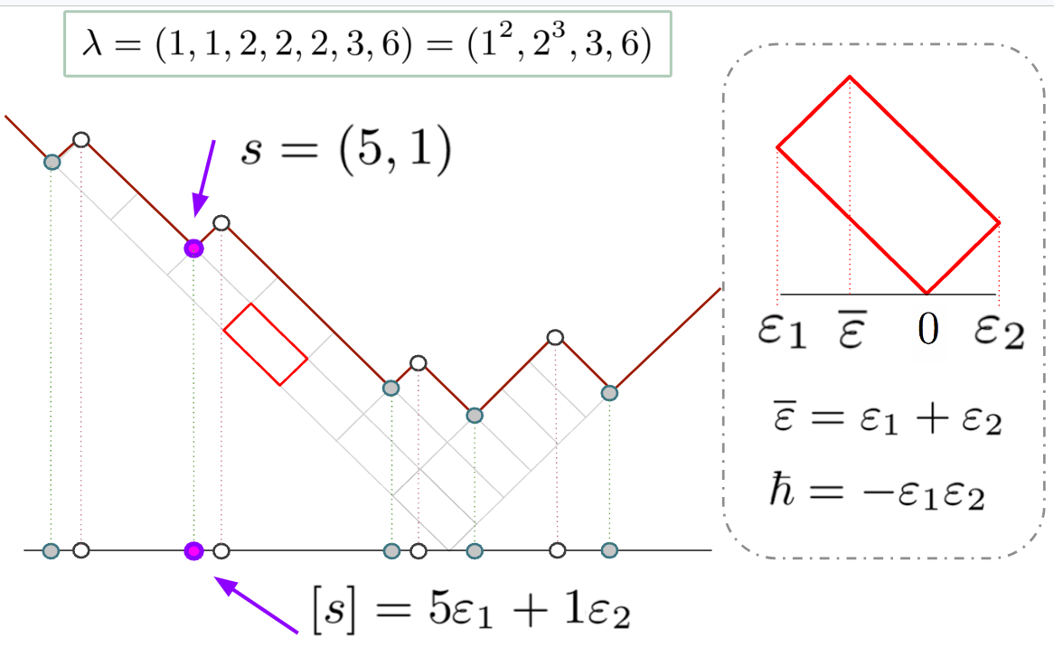
Figure 1. The basic objects of our notation for partitions.

2.1.2. Symmetric Functions

We refer to the canonical source [9] for all foundational results. Consider the ring of symmetric functions $\Lambda:={\mathbb{C}}[x_{i}]^{\mathfrak{S}}$ in infinitely many variables $x_{i}$. Define the power sum symmetric functions as $p_{k}=\sum_{i}{x_{i}^{k}}$. For $\mu=(\mu_{1},\mu_{2},\ldots)$ a partition, we write $p_{\mu}=\prod_{k}p_{\mu_{k}}$, and denote the monomial symmetric functions $m_{\mu}=x^{\mu}+\ldots$. . For $\alpha\in{\mathbb{R}}$, we define the $\alpha$-deformed Hall inner product, by

(10) $$\langle p_{\mu},p_{\nu}\rangle_{\alpha}:=\delta_{\mu,\nu}z_{\mu}\alpha^{|\mu|},\text{ where }z_{\mu}=\prod_{k}(\mu_{k}!\,k^{\mu_{k}}).$$

2.1.3. Jack Functions

Define the real deformation parameter $\alpha=-{\varepsilon}_{2}/{\varepsilon}_{1}$. The (integral form) Jack symmetric functions $J_{\lambda}^{(\alpha)}$, indexed by partitions $\lambda$, are a family of symmetric functions depending on the deformation parameter $\alpha$, introduced in [7]. When $\alpha=1$, these reduce to the standard Schur symmetric functions $s_{\lambda}$.

Proposition 2.1 (Jack Functions [9] Chap. VI, (4.5)).

There exists a unique family of symmetric functions $J_{\lambda}\in\Lambda[\alpha]$, indexed by partitions $\lambda$, which satisfy the following three properties

• Orthogonality:

  (11) $$\langle J_{\lambda},J_{\mu}\rangle_{\alpha}=0\text{ when }\lambda\neq\mu.$$

• Triangularity:

  (12) $$J_{\lambda}=\sum_{\mu<_{d}\lambda}c_{\lambda\mu}m_{\mu},$$

  where $<_{d}$ indicates dominance order on partitions.

• Normalization:

  (13) $$[m_{1^{n}}]J_{\lambda}=n!.$$

This normalization is known as the integral form of the Jack symmetric functions, as they have the property that $J_{\lambda}^{(\alpha)}\in{\mathbb{Z}}[\alpha,p_{1},p_{2},\ldots]$ in the basis of the power-sum symmetric functions with the expansion

(14) $$J_{\lambda}^{(\alpha)}=1.p_{1}^{|\lambda|}+\ldots$$

For example, for partitions of size $n=3$, the Jack functions are

(15) $$J_{\{1^{3}\}}^{(\alpha)}(p)= p_{1}^{3}-3p_{2}p_{1}+2p_{3} =6m_{1^{3}},$$

(16) $$J_{\{1,2\}}^{(\alpha)}(p)= p_{1}^{3}+(\alpha-1)p_{2}p_{1}-\alpha p_{3} =6m_{1^{3}}+(\alpha+2)m_{1,2},$$

(17) $$J_{\{3\}}^{(\alpha)}(p)= p_{1}^{3}+3\alpha p_{2}p_{1}+2\alpha^{2}p_{3} =6m_{1^{3}}+3(\alpha+1)m_{1,2}+(\alpha+1)(2\alpha+1)m_{3}.$$

The triangularity of the Jack functions in the monomial basis is evident.

2.1.4. Fock Module

We use the ring of coefficients ${{\mathbb{C}}_{{\bm{{\varepsilon}}}}}={\mathbb{C}}({\varepsilon}_{1},{\varepsilon}_{2})$. Out of the two deformation parameters, we build two secondary parameters: The quantum parameter $\hbar=-{\varepsilon}_{1}{\varepsilon}_{2}=-[(1,0)][(0,1)]$, and the dispersion parameter ${\overline{\varepsilon}}={\varepsilon}_{1}+{\varepsilon}_{2}=[(1,1)]$. We consider a $\hat{\mathfrak{gl}}_{1}$ Heisenberg current $V(z)=\sum_{k}V_{k}z^{k}$, with $V_{0}=0$ and $[V_{n},V_{m}]=\hbar n\delta_{n+m,0}$. This current acts on the Fock module ${\mathcal{F}}={{\mathbb{C}}_{{\bm{{\varepsilon}}}}}[V_{1},V_{2},\cdots]$, via

(18) $$V_{-k}=\hbar k\partial_{V_{k}},\quad k>0.$$

In this paper, we work with an alternate presentation of the ring of symmetric functions by embedding them into the Fock module via $p_{k}\to(-{\varepsilon}_{1})^{-1}V_{k}$. In this basis, the Hall inner product becomes

(19) $$||V_{1}^{d_{1}}V_{2}^{d_{2}}\cdots||_{\hbar}^{2}=\prod_{k=1}^{\infty}(\hbar k)^{d_{k}}d_{k}!.$$

With this, we have

(20) $$V_{-k}=V_{k}^{\dagger}.$$

This ring has the natural grading operator ${\mathcal{N}}$, where $V_{k}$ has degree $k$.

2.1.5. Homogeneous Integral Normalization

We will use homogeneous normalization of the integral Jack functions (henceforth denoted with a lower case $j$), considered as elements in the Fock module ${\mathcal{F}}$, given by:

(21) $$j_{\lambda}(V|{\varepsilon}_{1},{\varepsilon}_{2}):={(-{\varepsilon}_{1})^{|\lambda|}}\cdot J^{(\alpha=-{\varepsilon}_{2}/{\varepsilon}_{1})}_{\lambda}(p=(-{\varepsilon}_{1})^{-1}V)\in{\mathcal{F}}.$$

With this normalization, the three homogeneous Jack functions for $n=3$ are given by

(22) $$j_{\{1^{3}\}}= V_{1}^{3}+3{\varepsilon}_{1}V_{1}V_{2}+2{\varepsilon}_{1}^{2}V_{3},$$

(23) $$j_{\{1,2\}}= V_{1}^{3}+({\varepsilon}_{1}+{\varepsilon}_{2})V_{1}V_{2}+{\varepsilon}_{1}{\varepsilon}_{2}V_{3},$$

(24) $$j_{\{3\}}= V_{1}^{3}+3{\varepsilon}_{2}V_{1}V_{2}+2{\varepsilon}_{2}^{2}V_{3}.$$

Note that these are all homogenous integral polynomials in ${\mathbb{Z}}[{\varepsilon}_{1},{\varepsilon}_{2},V_{1},V_{2},\ldots]$, and that in this normalization we have the explicit transpositional symmetry:

(25) $$j_{\lambda}(V|{\varepsilon}_{1},{\varepsilon}_{2})=j_{\lambda^{\prime}}(V|{\varepsilon}_{2},{\varepsilon}_{1}).$$

Lemma 2.2 (Principal Specialization [15] Thm 5.4).

For a partition $\lambda$, we have

(26) $$j_{\lambda}(V_{i}=z)=\prod_{b\in\lambda}(z+[b]),$$

and hence

(27) $$\varpi_{\lambda}:=[V_{n}]j_{\lambda}=\prod_{b\in\lambda^{\times}}[b].$$

2.1.6. Jack Littlewood-Richardson (LR) Coefficients

Much of the work in this paper will be concerning the Jack Littlewood-Richardson coefficients, $c_{\mu,\nu}^{\lambda}$, defined as the expansion coefficients in the product of Jack functions,

(28) $$j_{\mu}\cdot j_{\nu}=\sum_{\lambda}c_{\mu,\nu}^{\lambda}\,j_{\lambda}.$$

In the literature, these are often denoted as $c_{\mu,\nu}^{\lambda}(\alpha)$ to indicate the dependence on the deformation parameter $\alpha$. In general, it is very difficult to find explicit closed-form expressions for these coefficients, instead most formulas involving them are recursive in nature. In this paper, we find new families of relations between these coefficients. In the sequel paper, [1], we make progress towards finding explicit closed form expressions.

The most well known explicit formula for Jack LR coefficients is given by

Proposition 2.3 (Pieri Rule - Stanley ’89 [15] Thm 6.1).

Let $\mu\subset\lambda$, and $\lambda/\mu$ be a horizontal $r$-strip, i.e. no two boxes in the quotient shape $\lambda/\mu$ are adjacent in a row. Then

(29) $$c_{1^{r},\mu}^{\lambda}=\frac{\left(\prod_{s\in\{1^{r}\}}h^{L}_{1^{r}}(s)\right)\left(\prod_{t\in\mu}A_{\mu}(t)\right)}{\left(\prod_{v\in\lambda}A_{\lambda}(v)\right)},$$

where

(30) $$A_{\sigma}(b)=h^{U}_{\sigma}(b)\text{ if $\lambda/\mu$ does not intersect the row of $b$, $h^{L}_{\sigma}(b)$ otherwise. }$$

2.2. The Nazarov-Skylanin Lax Operator

In this section, we recall the work of the previous paper in this series, [10], which explores the extraordinary quantum Lax operator introduced by Nazarov-Skylanin in [11].

2.2.1. Preliminaries

We enlarge our Hilbert space and work in the extended Fock module ${\mathcal{H}}={\mathcal{F}}\otimes{\mathbb{C}}[w]$, where $w$ is of degree 1. The inner product is

(31) $$\langle V_{\mu}w^{m},V_{\nu}w^{n}\rangle=\delta_{n,m}\langle V_{\mu},V_{\nu}\rangle_{\hbar}.$$

In this way, the inclusion ${\mathcal{F}}\hookrightarrow{\mathcal{H}}$ is an isometry. The total grading operator for ${\mathcal{H}}$ is

(32) $${\mathcal{N}}^{*}:={\mathcal{N}}+w\partial_{w}=\hbar^{-1}\sum_{k>0}V_{k}V_{-k}+w\partial_{w}.$$

This gives the graded decomposition

(33) $${\mathcal{H}}=\bigoplus_{n\geq 0}{\mathcal{H}}_{n}.$$

On this space, we have several important projections on ${\mathcal{H}}$. Firstly, $\pi_{0}:{\mathcal{H}}\to{\mathcal{F}}\subset{\mathcal{H}}$ projects just onto the $w^{0}$ component. $\pi_{+}$ is its complement, projecting only onto positive powers of $w$. $\pi_{w}:F[w,w^{-1}]\to F[w]$ is the map that projects onto non-negative powers of $w$.

2.2.2. Lax Operator

We at last come to introducing the main actor in our story.

Definition 2.4.

The Nazarov-Sklyanin Lax Operator [11] is the linear operator on ${\mathcal{H}}={\mathcal{F}}[w]$ given by

(34) $${\mathcal{L}}=\pi_{w}\sum_{k>0}\left(w^{-k}V_{k}+w^{k}V_{-k}\right)+{\overline{\varepsilon}}w\partial_{w}$$

In the basis ${\mathcal{H}}=\oplus_{k}(w^{k}{\mathcal{F}})$, we can express ${\mathcal{L}}$ as the semi-infinite matrix operator, with coefficients in $\mathop{\rm End}({\mathcal{F}})$,

(35) $${\mathcal{L}}:=\left(\begin{matrix}0&V_{1}&V_{2}&V_{3}&\cdots\\ V_{-1}&{\overline{\varepsilon}}&V_{1}&V_{2}&\cdots\\ V_{-2}&V_{-1}&2{\overline{\varepsilon}}&V_{2}&\cdots\\ V_{-3}&V_{-2}&V_{-1}&3{\overline{\varepsilon}}&\cdots\\ \vdots&\vdots&\vdots&\vdots&\ddots\\ \end{matrix}\right)$$

One can check that ${\mathcal{L}}$ commutes with grading operator 32, so let ${\mathcal{L}}_{n}={\mathcal{L}}|_{{\mathcal{H}}_{n}}$. Furthermore, let ${\mathcal{L}}^{+}=\pi_{+}{\mathcal{L}}|_{{\mathcal{H}}_{+}}$ be the restrictions of ${\mathcal{L}}$ to only the positive powers of $w$.

Corollary 2.5 (Shift property).

(36) $$w^{-1}{\mathcal{L}}_{n+1}^{+}w={\mathcal{L}}_{n}+{\overline{\varepsilon}}$$

Note that from the definition 34 its clear that ${\mathcal{L}}$ acts as derivation if either of the factors is in ${\mathcal{H}}^{0}:=\pi_{0}{\mathcal{H}}={\mathcal{F}}$, i.e.

(37) $${\mathcal{L}}(\zeta\cdot\xi)={\mathcal{L}}(\zeta)\cdot\xi+\zeta\cdot{\mathcal{L}}(\xi),\qquad\text{ if }\zeta\in{\mathcal{H}}^{0}.$$

2.2.3. Spectral Factors I

We will make extended use of the following rational functions that are associated to partitions $\lambda$.

(38) $$T_{\lambda}(u):=\prod_{s\in\lambda}N(u-[s]),\qquad\text{ where }N(u)=\frac{(u-[0,0])(u-[1,1])}{(u-[1,0])(u-[0,1])}.$$

For example, in the simplest case $T_{1}(u)$ has a zero at the top and bottom corners and poles at each of the side corners, illustrated in figure 2.

Figure 2. $T_{1}(u)=N(u)=\frac{(u-[0,0])(u-[1,1])}{(u-[1,0])(u-[0,1])}$.

Figure 3. $T_{\{1,2\}}(u)=N(u)N(u-[1,0])N(u-[0,1])=\frac{(u-[0,0])(u-[2,1])(u-[1,2])}{(u-[2,0])(u-[1,1])(u-[0,2])}$.

Note that we have the cancellations of poles and zeros on the internal corners of the partition, and we are left with poles at the ‘inner’ corners, and zeros at the ‘outer’ corners, that is,

(39) $$T_{\lambda}(u)=u\cdot\frac{\prod_{t\in\mathcal{R}^{+}_{\lambda}}(u-[t])}{\prod_{s\in\mathcal{A}_{\lambda}}(u-[s])}.$$

2.2.4. Integrable Hierarchy

We consider the following ‘transfer’ operator for ${\mathcal{L}}$,

(40) $${\mathcal{T}}(u):=\pi_{0}(u-{\mathcal{L}})^{-1}:\mathop{\rm End}({\mathcal{F}})\otimes{\mathbb{C}}(u).$$

The motivating result for most of this work is the following remarkable property of the Lax operator ${\mathcal{L}}$.

Theorem 2.6 ( Nazarov-Sklyanin (2013) [11] ).

The transfer operator ${\mathcal{T}}(u)$ is diagonalized on the homogenous Jack functions $j_{\lambda}\in{\mathcal{F}}$,

(41) $${\mathcal{T}}(u)\,j_{\lambda}=u^{-1}T_{\lambda}(u)\cdot j_{\lambda}$$

where $T_{\lambda}(u)$ is the spectral factor 38.

2.2.5. Transition Measures

The influential work of Kerov [8] introduces the following objects.

Definition 2.7 ([8] eq. (3.1)).

For $s\in\mathcal{A}_{\lambda}$, define the co-transition measure

(42) $$\tau_{\lambda}^{s}:=\mathop{\rm Res}_{u=[s]}u^{-1}T_{\lambda}(u)=\frac{\prod_{t\in\mathcal{R}^{+}_{\lambda}}[s-t]}{\prod_{s^{\prime}\in\mathcal{A}_{\lambda},s^{\prime}\neq s}[s-s^{\prime}]}.$$

Note that for ${\varepsilon}_{2}<0<{\varepsilon}_{1}$, it can be shown that $\tau_{\lambda}^{s}>0$ and $\sum_{s\in\mathcal{A}_{\lambda}}\tau_{\lambda}^{s}=1$, hence these coefficients define a probability measure on the add-set of $\lambda$. A connection between these measures and Jack LR coefficients was shown by Kerov.

Lemma 2.8 (Kerov ’97 [8] thm. (6.7)).

The simplest Jack LR coefficient coincides with the co-transition measure,

(43) $$c_{1,\lambda}^{\lambda+s}=\tau_{\lambda}^{s}.$$

That is, Jack functions satisfy the following simple multiplication formula (‘Pieri’ rule)

(44) $$j_{1}\cdot j_{\lambda}=\sum_{s\in\mathcal{A}_{\lambda}}\tau_{\lambda}^{s}\,j_{\lambda+s}.$$

From this, we can write

(45) $$u^{-1}T_{\lambda}(u)=\sum_{s\in\mathcal{A}_{\lambda}}c_{1,\lambda}^{\lambda+s}\frac{1}{u-[s]}.$$

One of the main results (Theorem 4.28) of this paper is a generalization this Kerov relation between Jack LR coefficients and residues of certain ‘spectral’ rational functions.

Kerov also introduces the transition measures, for $t\in\mathcal{R}^{+}_{\lambda}$,

(46) $$\tilde{\tau}^{t}_{\lambda}=\mathop{\rm Res}_{u=[t]}u\,T_{\lambda}(u)^{-1}.$$

2.3. Spectral Theorem

Here we recall the results of Mickler-Moll [10] on the spectrum of the Nazarov-Skylanin Lax operator. Fix $n\in{\mathbb{N}}$. Consider the ${\mathcal{L}}$-cyclic subspaces of ${\mathcal{H}}_{n}$ generated by the Jack polynomials $j_{\lambda}\in{\mathcal{H}}_{n}^{0}$.

Definition 2.9.

The "Jack-Lax" cyclic subspaces of $j_{\lambda}$ under ${\mathcal{L}}_{n}$ are denoted by

(47) $${{Z}}_{\lambda}:=Z(j_{\lambda},{\mathcal{L}}_{n})\subset{\mathcal{H}}_{n}.$$

One immediate corollary of the NS theorem (41) in this language is

Corollary 2.10.

$\pi_{0}{{Z}}_{\lambda}=j_{\lambda}$.

We can now state the main result of the first paper in this series.

Theorem 2.11 (Spectral Decomposition [10]).

 

• Under the action of the Nazarov-Skylanin Lax operator ${\mathcal{L}}$, the space ${\mathcal{H}}_{n}$ has the following cyclic decomposition

  (48) $${\mathcal{H}}_{n}=\bigoplus_{\lambda\,\vdash\,n}{{Z}}_{\lambda}.$$

  under which ${\mathcal{L}}$ acts in block diagonal form ${\mathcal{L}}=\oplus{\mathcal{L}}_{\lambda}$, where ${\mathcal{L}}_{\lambda}={\mathcal{L}}_{n}|{{Z}}_{\lambda}$.

• The eigenfunctions of ${\mathcal{L}}_{\lambda}$ on ${{Z}}_{\lambda}$ are labelled $\{\psi_{\lambda}^{s}:s\in\mathcal{A}_{\lambda}\}$ with eigenvalues given by the corresponding box content

  (49) $${\mathcal{L}}\,\psi_{\lambda}^{s}=[s]\cdot\psi_{\lambda}^{s}.$$

  Thus, the cyclic subspace ${{Z}}_{\lambda}$ is given as

  (50) $${{Z}}_{\lambda}=\mathop{\rm Span}_{s\in\mathcal{A}_{\lambda}}\{\psi_{\lambda}^{s}\}\subset{\mathcal{H}}_{n}.$$

• The eigenfunctions of ${\mathcal{L}}_{\lambda}^{+}$ on ${{Z}}_{\lambda}^{+}:=\pi_{+}{{Z}}_{\lambda}$ are labelled $\{\tilde{\psi}_{\lambda}^{t}:t\in\mathcal{R}^{+}_{\lambda}\}$ with eigenvalues given by the corresponding box content

  (51) $${\mathcal{L}}^{+}\,\tilde{\psi}_{\lambda}^{t}=[t]\cdot\tilde{\psi}_{\lambda}^{t}.$$

• These eigenfunctions can be normalized to satisfy

  (52) $$\pi_{0}\psi_{\lambda}^{s}=j_{\lambda},\qquad\tilde{\psi}_{\lambda}^{t}=\frac{1}{[t]-{\mathcal{L}}}j_{\lambda}.$$

  With this normalization, we have

  (53) $$j_{\lambda}=\sum_{s\in\mathcal{A}_{\lambda}}\tau_{\lambda}^{s}\psi_{\lambda}^{s}\in{{Z}}_{\lambda},\quad\text{ where }\quad\tau_{\lambda}^{s}:=\mathop{\rm Res}_{u=[s]}\left(u^{-1}T_{\lambda}(u)\right).$$

(54) $${\mathcal{L}}_{n}j_{\lambda}=\sum_{t\in\mathcal{R}^{+}_{\lambda}}{\tilde{\tau}}_{\lambda}^{t}{\tilde{\psi}}_{\lambda}^{t}\in{{Z}}_{\lambda}^{+},\quad\text{ where }\quad{\tilde{\tau}}_{\lambda}^{t}:=\mathop{\rm Res}_{u=[t]}\left(uT_{\lambda}(u)^{-1}\right).$$

We also recall the following useful result:

Lemma 2.12 (Principal Specialization [10]).

(55) $$\psi_{\lambda}^{s}(z,1)=\prod_{b\in(\lambda+s)^{\times}}(z+[b]),$$

and hence

(56) $$[w^{|\lambda|}]\psi_{\lambda}^{s}(V,w)=[s]\varpi_{\lambda}.$$

3. Three Decompositions

In this section, we begin the new work of this paper.

As mentioned in the introduction, our primary objective will be to provide a new approach the classical problem of understanding the structure coefficients of products of Jack functions

(57) $$j_{\lambda}\cdot j_{\nu}=\sum_{\gamma}c_{\lambda,\nu}^{\gamma}j_{\gamma}.$$

The central claim of this paper is that by considering the structure of the algebra of Lax eigenfunctions

(58) $$\psi_{\lambda}^{s}\cdot\psi_{\nu}^{t}=\sum_{\gamma,u}c_{\lambda,\nu;u}^{s,t;\gamma}\psi_{\gamma}^{u},$$

we will gain insight into the products of Jack functions. The Jack-Lax Littlewood-Richardson coefficients, $c_{\lambda,\nu;u}^{s,t;\gamma}$, will be illuminated throughout this paper. This algebra reproduces the Jack LR coefficients under the projection to $\pi_{0}$, and hence

(59) $$c_{\lambda,\nu}^{\gamma}=\sum_{u\in\mathcal{A}_{\gamma}}c_{\lambda,\nu;u}^{s,t;\gamma}.$$

We will build up towards goal of understanding these Jack-Lax LR coefficients, by first developing a structural theory for $\psi_{\lambda}^{s}$.

3.1. Norm Formulae

We recall an important formula of Stanley for the norm squared of Jack functions.

Proposition 3.1 (Stanley [15] Thm 5.8).

(60) $$|j_{\lambda}|^{2}=\prod_{b\in\lambda}h^{U}_{\lambda}(b)h_{\lambda}^{L}(b)$$

We next prove a similar formula for Lax eigenfunctions. Let $c_{b}(\lambda)$ (resp. $r_{b}(\lambda)$) be the subset of boxes of $\lambda$ that are in the same column (resp. row) as $b$.

Lemma 3.2 ($\psi$ Norm Formula).

(61) $$|\psi_{\lambda}^{s}|^{2}=\prod_{b\in\lambda}C^{U}_{\lambda,s}(b)C_{\lambda,s}^{L}(b)$$

where

(62) $$C^{U}_{\lambda,s}(b)=h^{U}_{\lambda}(b)\text{ if $b\notin c_{s}(\lambda)$, $h^{U}_{\lambda+s}(b)$ otherwise. }$$

(63) $$C^{L}_{\lambda,s}(b)=h^{L}_{\lambda}(b)\text{ if $b\notin r_{s}(\lambda)$, $h^{L}_{\lambda+s}(b)$ otherwise. }$$

Proof.

As observed in the first paper in this series, the two ways of expanding the expression $\langle\psi_{\lambda}^{s},j_{\lambda}\rangle$ lead to the formula

(64) $$|\psi_{\lambda}^{s}|^{2}=\frac{|j_{\lambda}|^{2}}{\tau_{\lambda}^{s}}.$$

Using Kerov’s identity 43 and Stanley’s Pieri formula 29, we get

(65) $$\tau_{\lambda}^{s}=c_{1,\lambda}^{\lambda+s}=\frac{h_{1}^{L}((0,0))\left(\prod_{b\in\lambda}A_{\lambda}(b)\right)}{\left(\prod_{b\in\lambda+s}A_{\lambda+s}(b)\right)}.$$

Expanding this out, the factors not in the row-column shared with $s$ cancel, and by using $h_{1}^{L}((0,0))=h_{\lambda+s}^{L}(s)$, we get

(66) $$\tau_{\lambda}^{s}=\frac{\left(\prod_{b\in r_{s}(\lambda)}h^{L}_{\lambda}(b)\right)}{\left(\prod_{b\in r_{s}(\lambda)}h^{L}_{\lambda+s}(b)\right)}\frac{\left(\prod_{b\in c_{s}(\lambda)}h^{U}_{\lambda}(b)\right)}{\left(\prod_{b\in c_{s}(\lambda)}h^{U}_{\lambda+s}(b)\right)},$$

and the result follows from 60. ∎

[CLAIM?]

$$\sum_{s}\tau_{\lambda}^{s}\prod_{b\in\lambda}C^{U}_{\lambda,s}(b)=\prod_{b\in\lambda}h^{U}_{\lambda,}(b)$$

Example 3.3.

We can compute (using $({\varepsilon}_{1},{\varepsilon}_{2})=(X,Y)$ for readability)

$$\psi_{1,2^{2}}^{(2,1)} = w^{0}(V_{1}^{5}+2(2X+Y)V_{1}^{3}V_{2}+(3X^{2}+XY+Y^{2})V_{2}^{2}V_{1}+2X(X+3Y)V_{1}^{2}V_{3}$$

$$\quad\quad+2X(X^{2}+Y^{2})V_{2}V_{3}+XY(7X+Y)V_{1}V_{4}+2X^{2}Y(X+Y)V_{5})+$$

$$w^{1}((2X+Y)V_{1}^{4}+2(3X^{2}+XY+Y^{2})V_{1}^{2}V_{2}+Y(5X^{2}-3XY+Y^{2})V_{2}^{2}$$

$$\quad\quad+4X(X^{2}+Y^{2})V_{1}V_{3}+XY(4X^{2}-XY+Y^{2})V_{4})+$$

$$w^{2}(2X(X+3Y)V_{1}^{3}+6X(X^{2}+Y^{2})V_{1}V_{2}+2X(2X^{2}-3XY+3Y^{2})V_{3})+$$

$$w^{3}(2XY(7X+Y)V_{1}^{2}+2XY(4X2-XY+Y^{2})V_{2})+$$

$$w^{4}(10X^{2}Y(X+Y)V_{1})+$$

$$w^{5}(2X^{2}Y(2X^{2}+3XY+Y^{2})).$$

We also use the Stanley Pieri formula (29) to compute,

(67) $$|j_{1,2^{2}}|^{2}=[1,0][2,-1][3,-1][1,0][2,0]\cdot[0,-1][1,-2][2,-2][0,-1][1,-1],$$

where we have grouped as L/U hooks. Then (using red to highlight the hooks that have changed), we have

(68) $$|\psi_{1,2^{2}}^{(2,1)}|^{2}={\color[rgb]{1,0,0}[1,-1]}[2,-1][3,-1][1,0][2,0]\cdot[0,-1][1,-2][2,-2]{\color[rgb]{1,0,0}[1,-1][2,-1]}.$$

3.2. Action of $w$

Next, we investigate the relationship between eigenvalues of different degrees via the action of multiplication by $w:{\mathcal{H}}_{n}\to{\mathcal{H}}_{n+1}$ in terms of the basis of Lax-eigenfunctions $\psi$. We begin with a ${\mathcal{L}}_{n}$ eigenfunction $\psi_{\gamma}^{t}$, for $\gamma\,\vdash\,n$. We note that the shift property $w^{-1}{\mathcal{L}}_{n+1}^{+}w={\mathcal{L}}_{n}+{\overline{\varepsilon}}$ (2.5), yields

(69) $${\mathcal{L}}^{+}_{n+1}\left(w\psi_{\gamma}^{t}\right)=w({\mathcal{L}}_{n}+{\overline{\varepsilon}})\psi_{\gamma}^{t}=[t+(1,1)]w\psi_{\gamma}^{t}.$$

That is, $w\psi_{\gamma}^{t}\in{\mathcal{H}}_{n+1}$ is in the $[t+(1,1)]$ eigenspace of ${\mathcal{L}}^{+}_{n+1}$. First, we determine precisely what eigenfunction this is, as this eigenspace is generically greater than one dimensional. The spectrum of ${\mathcal{L}}^{+}_{n+1}$ was provided in the spectral theorem 2.11.

Theorem 3.4 (Shift Theorem).

We have followed equality of eigenfunctions of ${\mathcal{L}}^{+}_{n+1}$,

(70) $$w\,\psi_{\gamma}^{t}=\tilde{\psi}_{\gamma+t}^{t+(1,1)}.$$

Proof.

We prove by induction on size of the partition $\gamma$. For the base case, we check $\tilde{\psi}_{1}^{(1,1)}=w=w\psi_{\emptyset}^{(0,0)}$. For the inductive step, assume equation (70) holds for all $\gamma$ with $|\gamma|\leq n$.

We begin with the Pieri rule (44), for $\lambda\,\vdash\,n$:

(71) $$j_{1}j_{\lambda}=\sum_{s\in\mathcal{A}_{\lambda}}\tau_{\lambda}^{s}\,j_{\lambda+s}.$$

We first act with ${\mathcal{L}}$ on both sides of this equation. In general ${\mathcal{L}}$ is not a derivation. However, when acting on terms of degree zero, it is (37). After dividing both sides by $w$, this yields

(72) $$q_{1}j_{\lambda}+j_{1}q_{\lambda}=\sum_{s\in\mathcal{A}_{\lambda}}\tau_{\lambda}^{s}\,q_{\lambda+s},$$

where we have used the following definition for $\gamma\,\vdash\,(n+1)$,

(73) $$q_{\gamma}:=w^{-1}{\mathcal{L}}_{n+1}j_{\gamma}\in{\mathcal{H}}_{n}.$$

Note, from 54 we have

(74) $$q_{\gamma}=\sum_{t\in\mathcal{R}_{\gamma}}\tilde{\tau}_{\gamma}^{t+(1,1)}w^{-1}\tilde{\psi}_{\gamma}^{t+(1,1)}\in\pi^{+}{\mathcal{H}}_{n+1}.$$

The strategy will be to hit both sides with the projector $P_{[s]}$ onto the $[s]$ eigenspace of ${\mathcal{L}}$, for a choice of $s\in\mathcal{A}_{\lambda}$, and equate the results.

On the right hand side of (72), the only term in the sum is not annihilated by the spectral projector $P_{[s]}$ is $q_{\lambda+s}$, since by (69) the eigenvalues appearing in the $\psi$ decomposition of some $q_{\gamma}$ are precisely $\{[t]:t\in\mathcal{R}_{\gamma}\}$, and only $\lambda+s$ has a maximum at $s+(1,1)$. Thus, only term that survives the projection is

(75) $$P_{[s]}q_{\lambda+s}=\tilde{\tau}_{\lambda+s}^{s+(1,1)}w^{-1}\tilde{\psi}^{s+(1,1)}_{\lambda+s}.$$

Now for the left hand side of (72), we expand

(76) $$q_{1}j_{\lambda}+j_{1}q_{\lambda}=\hbar\sum_{u\in\mathcal{A}_{\lambda}}\tau_{\lambda}^{u}\psi_{\lambda}^{u}+j_{1}w^{-1}\sum_{t\in\mathcal{R}_{\lambda}}\tilde{\tau}_{\lambda}^{t}\tilde{\psi}^{t+(1,1)}_{\lambda}.$$

We then use the inductive hypothesis, $w^{-1}\tilde{\psi}_{\lambda}^{t+(1,1)}=\psi_{\lambda-t}^{t}$, to rewrite the last term in this expression

(77) $$\hbar\sum_{u\in\mathcal{A}_{\lambda}}\tau_{\lambda}^{u}\psi_{\lambda}^{u}+j_{1}\sum_{t\in\mathcal{R}_{\lambda}}\tilde{\tau}_{\lambda}^{t}\psi^{t}_{\lambda-t}.$$

To expand this further, we need to explicitly expand out $j_{1}\cdot\psi_{\lambda-t}^{t}$. We first note that from the derivation property 37, we have

(78) $$({\mathcal{L}}-[t])\left(j_{1}\cdot\psi_{\lambda-t}^{t}\right)=\hbar\,w\,\psi_{\lambda-t}^{t}.$$

This tells us that

(79) $$j_{1}\cdot\psi_{\lambda-t}^{t}=({\mathcal{L}}-[t])^{-1}\hbar\,w\,\psi_{\lambda-t}^{t}+r^{t},$$

where $r^{t}$ is the $[t]$ eigenspace of ${\mathcal{L}}$. We use the inductive hypothesis a second time, in conjunction with the formula (52), to write

(80) $$w\,\psi_{\lambda-t}^{t}=\tilde{\psi}_{\lambda}^{t+(1,1)}=\frac{1}{[t+(1,1)]-{\mathcal{L}}}j_{\lambda}=\sum_{s\in\mathcal{A}_{\lambda}}\frac{1}{[t+(1,1)-s]}\tau_{\lambda}^{s}\psi^{s}_{\lambda}$$

So we find

(81) $$j_{1}\cdot\psi_{\lambda-t}^{t}=\sum_{s\in\mathcal{A}_{\lambda}}\frac{\hbar\,\tau_{\lambda}^{s}}{[t-s][t+(1,1)-s]}\psi^{s}_{\lambda}+r^{t}$$

But we are not yet done. We decompose the term $r^{t}$ it into its ${{Z}}_{\gamma}$ components,

(82) $$r^{t}=\sum_{\gamma\,:\,t\in\mathcal{A}_{\gamma}}r_{\gamma}\psi_{\gamma}^{t},\quad r_{\gamma}\in{\mathbb{C}}.$$

We know only a single $\psi$ can appear in each ${{Z}}_{\gamma}$, since the spectrum of ${\mathcal{L}}_{\gamma}:={\mathcal{L}}|_{{{Z}}_{\gamma}}$ is multiplicity free. Note that no ${{Z}}_{\lambda}$ component appears in this decomposition of $r^{t}$, since $t$ is not in $\mathcal{A}_{\lambda}$. Rather, all the ${{Z}}_{\lambda}$ components in equation (81) are in the first term on the right hand side. We now apply $\pi_{0}$ to (81) after using the decomposition (82), to get

(83) $$j_{1}\cdot j_{\lambda-t} = \left(\sum_{s\in\mathcal{A}_{\lambda}}\frac{\hbar\,\tau_{\lambda}^{s}}{[t-s][t+(1,1)-s]}\right)j_{\lambda}+\sum_{\gamma\,:\,t\in\mathcal{A}_{\gamma}}r_{\gamma}j_{\gamma}$$

(84) $$= \tau_{\lambda-t}^{t}j_{\lambda}+\sum_{\gamma\,:\,t\in\mathcal{A}_{\gamma}}r_{\gamma}j_{\gamma}$$

where we have used the identity (470) to evaluate the coefficient of $j_{\lambda}$. Comparing this result with the Pieri rule (44), we can read off the $r_{\gamma}$ coefficients to give us

(85) $$r^{t}=\sum_{u\in\mathcal{A}_{\lambda-t},u\neq t}\tau_{\lambda-t}^{u}\psi^{t}_{\lambda-t+u}.$$

After all this we find the explicit expression we sought

(87) $$j_{1}\cdot\psi_{\lambda-t}^{t} = \sum_{v\in\mathcal{A}_{\lambda}}\frac{\hbar\,\tau_{\lambda}^{v}}{[t-v][t+(1,1)-v]}\psi^{v}_{\lambda}$$

$$+\sum_{u\in\mathcal{A}_{\lambda-t},u\neq t}\tau_{\lambda-t}^{u}\psi^{t}_{\lambda-t+u}.$$

Plugging all this back into (77) we find

(90) $$q_{1}j_{\lambda}+j_{1}q_{\lambda} = \hbar\sum_{u\in\mathcal{A}_{\lambda}}\tau_{\lambda}^{u}\psi_{\lambda}^{u}$$

$$+\sum_{t\in\mathcal{R}_{\lambda}}\tilde{\tau}_{\lambda}^{t+(1,1)}\sum_{v\in\mathcal{A}_{\lambda}}\frac{\hbar\,\tau_{\lambda}^{v}}{[t-v][t-v]}\psi^{v}_{\lambda}$$

$$+\sum_{t\in\mathcal{R}_{\lambda}}\tilde{\tau}_{\lambda}^{t+(1,1)}\sum_{u\in\mathcal{A}_{\lambda-t},u\neq t}\tau_{\lambda-t}^{u}\psi^{t}_{\lambda-t+u}.$$

Because $s\in\mathcal{A}_{\lambda}$ can not be of the form $t$ for any $t\in\mathcal{R}_{\lambda}$, we can see that the only eigenfunction with eigenvalue $[s]$ for our specific choice of $s\in\mathcal{A}_{\lambda}$ that can appear on the left hand side is $\psi_{\lambda}^{s}$, with coefficient

(91) $$P_{[s]}\left(q_{1}j_{\lambda}+j_{1}q_{\lambda}\right) = \tau_{\lambda}^{s}\left(\hbar+\sum_{t\in\mathcal{R}_{\lambda}}\tilde{\tau}_{\lambda}^{t+(1,1)}\frac{\hbar}{[t-s][t+(1,1)-s]}\right)\psi_{\lambda}^{s}$$

(92) $$= \tau_{\lambda}^{s}\left(\tilde{\tau}_{\lambda+s}^{s+(1,1)}\right)\psi_{\lambda}^{s}$$

where we have used the identity (471) to evaluate the sum.

Thus, the result of hitting equation (72) with $P_{[s]}$ is the equality,

(93) $$\tau_{\lambda}^{s}\tilde{\tau}_{\lambda+s}^{s+(1,1)}\psi_{\lambda}^{s}=\tau_{\lambda}^{s}\tilde{\tau}_{\lambda+s}^{s+(1,1)}w^{-1}\tilde{\psi}^{s+(1,1)}_{\lambda+s},$$

That is, $w\cdot\psi_{\lambda}^{s}=\tilde{\psi}^{s+(1,1)}_{\lambda+s}$. Seeing as $s\in\mathcal{A}_{\lambda}$ was arbitrary, we find that equation (70) holds for all $\gamma\,\vdash\,(n+1)$, and so we have completed the inductive step. ∎

With this result, we no longer need to mention the eigenvalues of ${\mathcal{L}}^{+}$, as they are determined by $w$ and the eigenvalues of ${\mathcal{L}}$. In this spirit, we use the result (80) to determine the action of $w$ in the $\psi$ basis,

Corollary 3.5.

The action of $w$ in the basis of Lax eigenfunctions $\psi$ is given by

(94) $$w\cdot\psi_{\lambda}^{t}=\sum_{s\in\mathcal{A}_{\lambda+t}}\frac{\tau_{\lambda+t}^{s}}{[s-t-(1,1)]}\psi_{\lambda+t}^{s}.$$

In the remainder of this paper, we will make use of the following elements that appeared in the above proof,

Definition 3.6.

Define the ‘quack’ polynomial

(95) $$q_{\gamma}:=w^{-1}{\mathcal{L}}_{n+1}j_{\gamma}\in{\mathcal{H}}_{n}.$$

Note that $q_{\gamma}\in{\mathcal{F}}[w]_{n}$ involve all powers of $w$, unlike $j_{\lambda}\in{\mathcal{F}}$ which are polynomials only in the $V_{k}$.

3.3. $w$-Jack Expansion

We define the $w$-Jack expansion coefficients $\varphi_{\lambda,\mu}^{s}\in{{\mathbb{C}}_{{\bm{{\varepsilon}}}}}$ by

(96) $$\psi_{\lambda}^{s}=\sum_{\mu}\varphi_{\lambda,\mu}^{s}w^{|\lambda|-|\mu|}j_{\mu}.$$

Lemma 3.7.

We have $\varphi_{\lambda,\mu}^{s}=0$ unless $\mu\subseteq\lambda$. Furthermore, for $s\in\mathcal{A}_{\lambda}$ and $t\in\mathcal{R}_{\lambda}$, we have

(97) $$\varphi_{\lambda,\lambda-t}^{s}=\frac{\tilde{\tau}^{t+(1,1)}_{\lambda}}{[s-t-(1,1)]}.$$

Lastly, let $SYT(\lambda/\mu)$ be the collection of of standard young tableau of skew-shape $\lambda/\mu$. That is, $\Sigma\in SYT(\lambda/\mu)$ is a collection of partitions $\Sigma=\{\sigma_{i}\}$ with $\mu=\sigma_{0}\subset\sigma_{1}\subset\cdots\subset\sigma_{N}=\lambda$, where $N=|\lambda|-|\mu|$, with $\sigma_{i+1}=\sigma_{i}+b_{i}$ differing by a single box $b_{i}$. Then we have

(98) $$\varphi_{\lambda,\mu}^{s}=\sum_{\Sigma\in SYT(\lambda/\mu)}\prod_{i=0}^{N-1}\varphi_{\sigma_{i+1},\sigma_{i}}^{b_{i+1}}$$

where $b_{N}=s$.

Proof.

From [10], we know that $\psi_{\lambda}^{s}=j_{\lambda}+\frac{1}{[s]-{\mathcal{L}}^{+}}wq_{\lambda}=j_{\lambda}+w\frac{1}{[s]-{\mathcal{L}}-{\overline{\varepsilon}}}q_{\lambda}$. Using 95 and 70, we have

(99) $$\psi_{\lambda}^{s}=j_{\lambda}+w\sum_{t\in\mathcal{R}_{\lambda}}\frac{\tilde{\tau}_{\lambda}^{t+(1,1)}}{[s-t-(1,1)]}\psi_{\lambda-t}^{t}.$$

Applying 99 recursively, we recover the result. ∎

Thus we can write the restricted summation expression:

(100) $$\psi_{\lambda}^{s}=\sum_{\mu\subseteq\lambda}\varphi_{\lambda,\mu}^{s}w^{|\lambda|-|\mu|}j_{\mu}.$$

Lemma 3.8.

(101) $$\psi_{1^{r}}^{s}=\sum_{k=0}^{r}\varphi_{1^{r},1^{k}}^{s}w^{r-k}j_{1^{k}},$$

where for $k<r$ we have

(102) $$\varphi_{1^{r},1^{k}}^{s}=[s]\prod_{b\in 1^{r}/1^{k+1}}[b].$$

Proof.

We have

(103) $$\varphi_{1^{r},1^{r-1}}^{s}=\frac{\tilde{\tau}^{(r,1)}_{\lambda}}{[s-(r,1)]}=\frac{-[0,1][r,0]}{[s-(r,1)]}=[s],$$

since $s$ is either $(0,1)$ or $(r,0)$. With this, the result follows from Lemma (3.7). ∎

Example 3.9.

$\psi_{1^{3}}^{s}=j_{1^{3}}+[s]wj_{1^{2}}+[s][2,0]w^{2}j_{1}+[s][2,0][1,0]w^{3}$.

3.4. Jack-Lax Littlewood-Richardson Coefficients

Here, we can state the first example of the Jack-Lax Littlewood-Richardson coefficients (58), by providing a refinement of the simplest Pieri rule (44),

Lemma 3.10.

(105) $$\psi^{v}_{1}\cdot\psi_{\lambda}^{s} = \sum_{u\in\mathcal{A}_{\lambda+s}}\frac{[-v][s-u-v+(1,1)]}{[s-u][s-u+(1,1)]}\,\tau_{\lambda+s}^{u}\psi^{u}_{\lambda+s}$$

$$+\sum_{t\in\mathcal{A}_{\lambda},t\neq s}\tau_{\lambda}^{t}\psi^{s}_{\lambda+t}.$$

Proof.

We note that $\psi^{v}_{1}=j_{1}+[v]w$. We combine the formula (87)

(107) $$j_{1}\cdot\psi_{\lambda}^{s} = \sum_{b\in\mathcal{A}_{\lambda+s}}\frac{\hbar\,\tau_{\lambda+s}^{b}}{[s-b][s+(1,1)-b]}\psi^{b}_{\lambda+s}$$

$$+\sum_{t\in\mathcal{A}_{\lambda},t\neq s}\tau_{\lambda}^{t}\psi^{s}_{\lambda+t},$$

with (94)

(108) $$[v]w\cdot\psi_{\lambda}^{s} = \sum_{b\in\mathcal{A}_{\lambda+s}}\frac{[v]\tau_{\lambda+s}^{b}}{[b-s-(1,1)]}\psi_{\lambda+s}^{b},$$

to see that the coefficient of $\tau_{\lambda+s}^{b}\psi^{b}_{\lambda+s}$ is

(109) $$\frac{\hbar}{[s-b][s+(1,1)-b]}+\frac{[v]}{[b-s-(1,1)]}=\frac{[v][(1,1)-v]-[v][s-b]}{[s-b][s+(1,1)-b]},$$

and the result follows. ∎

If we apply $\pi_{0}$ to this formula, we recover the usual Pieri rule (44).

3.5. ${{X}}{{Y}}{{Z}}$ Decomposition

One of the ways we will gain insight into the structure of the algebra 58 is through various decompositions of the space ${\mathcal{H}}$. The first of these is given by the subspaces ${{Z}}_{\lambda}:=\mathop{\rm Span}_{s\in\mathcal{A}_{\lambda}}\{\psi_{\lambda}^{s}\}\subset{\mathcal{H}}_{|\lambda|}$, that is,

(110) $${\mathcal{H}}_{n}=\bigoplus_{\lambda\,\vdash\,n}{{Z}}_{\lambda}.$$

Example 3.11.

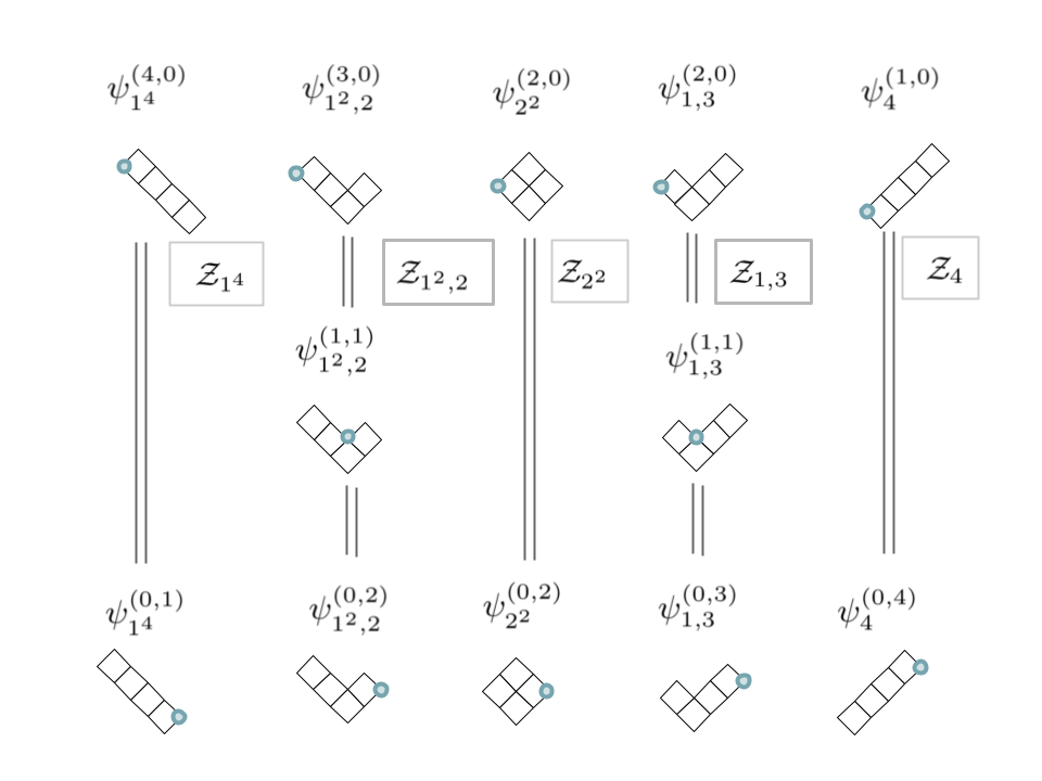
Figure 4. The decomposition ${\mathcal{H}}_{n}=\bigoplus_{\lambda\,\vdash\,n}{{Z}}_{\lambda}$, where vertical double lines represent ${{Z}}$ subspaces. For example, ${{Z}}_{2^{2}}=\mathop{\rm Span}\{\psi^{(2,0)}_{2^{2}},\psi_{2^{2}}^{(0,2)}\}\subset{\mathcal{H}}_{4}$.

The second decomposition of ${\mathcal{H}}$ is the eigen-decomposition under the Lax operator ${\mathcal{L}}$. Denote the $[s]$ eigenspace of ${\mathcal{L}}_{n}$ on ${\mathcal{H}}_{n}$ as ${{Y}}^{s}_{n}$. We then have

(111) $${\mathcal{H}}_{n}=\bigoplus_{s:\,[s]\in{\mathrm{Spec}}{\mathcal{L}}_{n}}{{Y}}_{n}^{s}.$$

Figure 5. The decomposition ${\mathcal{H}}_{n}=\bigoplus_{s:\,[s]\in{\mathrm{Spec}}{\mathcal{L}}_{n}}{{Y}}_{n}^{s}$, where horizontal lines represent ${{Y}}$ spaces. For example, ${{Y}}_{4}^{(2,0)}=\mathop{\rm Span}\{\psi^{(2,0)}_{1,3},\psi_{2^{2}}^{(2,0)}\}\subset{\mathcal{H}}_{4}$.

Motivated by the results of the previous section, we define the third decomposition into subspaces

Definition 3.12.

(112) $${{X}}_{\gamma}:=\mathop{\rm Span}_{t\in\mathcal{R}_{\gamma}}\{\psi_{\gamma-t}^{t}\}\subset{\mathcal{H}}_{|\gamma|-1}$$

These spaces also give a decomposition of ${\mathcal{H}}$.

Corollary 3.13.

(113) $${\mathcal{H}}_{n}=\bigoplus_{\gamma\,\vdash\,(n+1)}{{X}}_{\gamma}.$$

Figure 6. The decomposition ${\mathcal{H}}_{n}=\bigoplus_{\gamma\,\vdash\,(n+1)}{{X}}_{\gamma}$, where diagonal colored lines represent ${{X}}$ spaces. For example, ${\mathcal{X}}_{1^{3},2}=\mathop{\rm Span}\{\psi^{(0,1)}_{1^{4}},\psi_{1^{2},2}^{(3,0)}\}\subset{\mathcal{H}}_{4}$.

With this definition, the results of the previous section can be re-stated in the following simple way.

Corollary 3.14.

For $\gamma\,\vdash\,(n+1)$, the ${{X}}$ spaces are also Lax orbits

(114) $${{X}}_{\gamma}=Z(q_{\gamma},{\mathcal{L}}_{n})\subset{\mathcal{H}}_{n}.$$

or equivalently,

(115) $$q_{\gamma}=\sum_{t\in\mathcal{R}_{\gamma}}\tilde{\tau}_{\gamma}^{t+(1,1)}\psi_{\gamma-t}^{t}\in{{X}}_{\gamma}.$$

Furthermore, multiplication by $w$,

(116) $$w:{{X}}_{\lambda}\to{{Z}}_{\lambda}^{+},$$

is an isomorphism.

If we let $\Pi=w^{-1}\pi_{+}:{\mathcal{H}}_{n}\to{\mathcal{H}}_{n-1}$, we have the inverse statement to 94

Lemma 3.15.

(117) $$\Pi\psi_{\lambda}^{s}=\sum_{t\in\mathcal{R}_{\lambda}}\frac{\tilde{\tau}_{\lambda}^{t+(1,1)}}{[t+(1,1)-s]}\psi_{\lambda-t}^{t}\in{{X}}_{\lambda}.$$

Proof.

We note from [10] (A.5.3) we have $\psi_{\lambda}^{s}=j_{\lambda}+\frac{1}{{\mathcal{L}}^{+}-[s]}wq_{\lambda}$, from which we find $\pi_{+}\psi_{\lambda}^{s}=w\frac{1}{{\mathcal{L}}+{\overline{\varepsilon}}-[s]}q_{\lambda}$. ∎

With these definitions, we can provide a lifting of the obvious identity $|\mathcal{A}_{\lambda}|=1+|\mathcal{R}_{\lambda}|$ to the level of vector spaces.

Corollary 3.16 (Structural Theorem).

(118) $${{Z}}_{\lambda}={\mathbb{C}}\,j_{\lambda}\oplus w\cdot{{X}}_{\lambda}.$$

We have shown that we have three decompositions of ${\mathcal{H}}$,

(119) $${\mathcal{H}}_{n}=\bigoplus_{\gamma\,\vdash\,n+1}{{X}}_{\gamma}=\bigoplus_{[s]\in{\mathrm{Spec}}{\mathcal{L}}_{n}}{{Y}}^{s}=\bigoplus_{\lambda\,\vdash\,n}{{Z}}_{\lambda}.$$

We note that intersection of any two of ${{Z}}_{\lambda},{{X}}_{\lambda+s}$ or ${{Y}}^{s}$ is the line ${\mathbb{C}}\cdot\psi_{\lambda}^{s}\subset{\mathcal{H}}_{n}$, and that the intersection of any two of any type of these subspaces is at most one dimensional.

3.5.1. ${\pi_{\diamond}}$ operator

For a brief interlude, we introduce another projection operator.

Lemma 3.17.

Let $A:=\pi_{0}{\mathcal{L}}_{n+1}w:{\mathcal{H}}_{n}\to\pi^{0}H_{n+1}$, and $B:=w^{-1}{\mathcal{L}}_{n+1}:{\mathcal{H}}_{n+1}^{0}\to{\mathcal{H}}_{n}$, then we have

(120) $$AB=n\hbar\,{{{\mathrm{Id}}}}_{\pi^{0}{\mathcal{H}}_{n+1}}.$$

Let ${\pi_{\diamond}}\in\mathop{\rm End}{\mathcal{H}}_{n}$ be defined by

(121) $${\pi_{\diamond}}:=(n\hbar)^{-1}BA.$$

Then ${\pi_{\diamond}}^{2}={\pi_{\diamond}}$, that is, ${\pi_{\diamond}}$ is a projection operator of rank $\dim\pi^{0}{\mathcal{H}}_{n+1}=p(n+1)$.

We have shown that $Bj_{\lambda}=q_{\lambda}$ and $Aq_{\lambda}=n\hbar j_{\lambda}$, indeed $A\psi_{\gamma-s}^{s}=j_{\gamma}$. Hence ${\pi_{\diamond}}$ preserves the ${{X}}$ decomposition of ${\mathcal{H}}_{n}$, and

(122) $${\pi_{\diamond}}|_{{{X}}_{\gamma}}=\pi_{q_{\gamma}},$$

that is, ${\pi_{\diamond}}$ restricted to ${{X}}_{\lambda}$ is rank one and is equal to the projection operator onto $q_{\lambda}$. Compare this to the companion statement

(123) $$\pi_{0}|_{{{Z}}_{\lambda}}=\pi_{j_{\lambda}}.$$

3.6. Traces

3.6.1. Top Powers

The results so far concern looking at $\pi_{0}$ of a resolvent, that is, in the lowest powers of $w$. In this section, we rather look at the top component in powers of $w$. For any $\zeta\in{\mathcal{H}}_{n}$, define

(124) $$\pi_{*}\zeta:=[w^{n}]\zeta=\langle w^{n},\zeta\rangle\in{{\mathbb{C}}_{{\bm{{\varepsilon}}}}}.$$

Lemma 3.18.

The highest and lowest $w$-components of the Lax resolvent acting on a Jack function are given by

(125) $$\frac{1}{u-{\mathcal{L}}}j_{\lambda}=u^{-1}T_{\lambda}(u)\cdot j_{\lambda}w^{0}+\cdots+\varpi_{\lambda}\left(T_{\lambda}(u)-1\right)\cdot w^{|\lambda|},$$

where $\varpi_{\lambda}\coloneqq[V_{|\lambda|}]j_{\lambda}$ as before (27).

Proof.

Recall from 41, we have $\pi_{0}\frac{1}{u-{\mathcal{L}}}j_{\lambda}=u^{-1}T_{\lambda}(u)\cdot j_{\lambda}$. We use $j_{\lambda}=\sum_{s\in\mathcal{A}_{\lambda}}\tau_{\lambda}^{s}\psi_{\lambda}^{s}$, and compute the top component

(126) $$\pi_{*}\frac{1}{u-{\mathcal{L}}}j_{\lambda} = \sum_{s\in\mathcal{A}_{\lambda}}\tau_{\lambda}^{s}\frac{1}{u-[s]}\pi_{*}\psi_{\lambda}^{s}$$

(127) $$= \varpi_{\lambda}\sum_{s\in\mathcal{A}_{\lambda}}\frac{[s]\tau_{\lambda}^{s}}{u-[s]}$$

(128) $$= \varpi_{\lambda}\left(\sum_{s\in\mathcal{A}_{\lambda}}\frac{u\,\tau_{\lambda}^{s}}{u-[s]}-\sum_{s\in\mathcal{A}_{\lambda}}\tau_{\lambda}^{s}\right)$$

(129) $$= \varpi_{\lambda}\left(T_{\lambda}(u)-1\right).$$

On the second line we used the principal specialization result (56) $\pi_{*}\psi_{\lambda}^{s}=[s]\varpi_{\lambda}$. ∎

To reorient the rest of our work towards working with these top powers of $w$, we introduce new conventions.

Definition 3.19.

Define the rescaled ‘hatted’ elements

(130) $${\hat{\psi}}_{\lambda}^{s}:=\psi_{\lambda}^{s}/\pi_{*}(\psi_{\lambda}^{s})=\psi_{\lambda}^{s}/[s]\varpi_{\lambda},\quad\hat{j}_{\lambda}:=j_{\lambda}/\varpi_{\lambda},\quad\hat{q}_{\lambda}:=q_{\lambda}/\varpi_{\lambda},$$

(131) $${\hat{\tau}}_{\lambda}^{s}:=[s]\tau_{\lambda}^{s}.$$

With these redefinitions we have

(132) $$\hat{j}_{\lambda}=\sum_{s\in\mathcal{A}_{\lambda}}{\hat{\tau}}_{\lambda}^{s}{\hat{\psi}}_{\lambda}^{s},\qquad\sum_{s\in\mathcal{A}_{\lambda}}{\hat{\tau}}_{\lambda}^{s}=0,\qquad\hat{q}_{\gamma}=\sum_{t\in\mathcal{R}_{\gamma}}\tilde{\tau}_{\gamma}^{t+(1,1)}{\hat{\psi}}^{t}_{\gamma-t}.$$

Example 3.20.

(133) $$\hat{j}_{\{2^{2}\}}=\frac{1}{{\varepsilon}_{1}{\varepsilon}_{2}({\varepsilon}_{1}+{\varepsilon}_{2})}V_{1}4+\frac{2}{{\varepsilon}_{1}{\varepsilon}_{2}}V_{1}^{2}V_{2}+\frac{{\varepsilon}_{1}^{2}-{\varepsilon}_{1}{\varepsilon}_{2}+{\varepsilon}_{2}^{2}}{{\varepsilon}_{1}{\varepsilon}_{2}({\varepsilon}_{1}+{\varepsilon}_{2})}V_{2}^{2}+\frac{4}{{\varepsilon}_{1}+{\varepsilon}_{2}}V_{1}V_{3}+V_{4}.$$

It is important to note that this normalization does not work in the Schur case, where $({\varepsilon}_{2},{\varepsilon}_{1})=(1,-1)$, since for any partition $\mu$ containing the box $(1,1)$, the factor $[1,1]={\varepsilon}_{1}+{\varepsilon}_{2}$ in $\varpi_{\mu}=\prod_{s\in\mu^{\times}}[s]$ vanishes. For the remainder of this article, we will assume that ${\varepsilon}_{1}+{\varepsilon}_{2}\neq 0$. We leave the investigation of Schur polynomials and ordinary Littlewood-Richardson coefficients via the ${\varepsilon}_{1}+{\varepsilon}_{2}\to 0$ degeneration of our methods and results to future research.

3.6.2. Trace functionals

We continue the shifting of emphasis in our investigation to the coefficients of top powers of $w$ by introducing the first of three trace functionals.

Definition 3.21.

The ${y}$-trace functional ${y}_{u}:{\mathcal{H}}_{n}\to{{\mathbb{C}}_{{\bm{{\varepsilon}}}}}(u)$, is given by

(134) $${y}_{u}(\zeta):=\pi_{*}\frac{1}{u-{\mathcal{L}}}\zeta.$$

With the above redefinitions, we can restate Lemma 3.18 concisely

Corollary 3.22.

(135) $${y}_{u}(\hat{j}_{\lambda})=T_{\lambda}(u)-1.$$

We note that this trace is closely associated with the ${{Y}}$ subspaces (the ${\mathcal{L}}$-eigenspaces). We extend this definition the following three families of linear functionals ${\mathcal{H}}_{n}\to{{\mathbb{C}}_{{\bm{{\varepsilon}}}}}$ associated to each of the three decompositions (119) of ${\mathcal{H}}$

Definition 3.23.

(136) $${x}_{\gamma}(\zeta)=\pi_{*}P_{{{X}}_{\gamma}}\zeta,\qquad{y}^{s}(\zeta)=\pi_{*}P_{{{Y}}^{s}}\zeta,\qquad{z}_{\lambda}(\zeta)=\pi_{*}P_{{{Z}}_{\lambda}}\zeta.$$

Note that we have ${y}^{s}(\zeta)=\mathop{\rm Res}_{u=[s]}{y}_{u}(\zeta)$.

Lemma 3.24.

The traces are given by the following expressions,

(137) $${x}_{\gamma}(\zeta)=\langle\frac{\hat{q}_{\gamma}}{|\hat{j}_{\gamma}|^{2}},\zeta\rangle,\qquad{y}_{u}(\zeta)=\langle\frac{1}{u-{\mathcal{L}}}w^{n},\zeta\rangle,\qquad{z}_{\lambda}(\zeta)=\langle\frac{w\hat{q}_{\lambda}}{|\hat{j}_{\lambda}|^{2}},\zeta\rangle.$$

Equivalently,

(138) $$\frac{\hat{q}_{\gamma}}{|\hat{j}_{\gamma}|^{2}}=\sum_{t\in\mathcal{R}_{\gamma}}\frac{{\hat{\psi}}_{\gamma-t}^{t}}{|{\hat{\psi}}_{\gamma-t}^{t}|^{2}},\qquad w^{n}=\sum_{\lambda}\frac{w\hat{q}_{\lambda}}{|\hat{j}_{\lambda}|^{2}},\qquad\frac{w\hat{q}_{\lambda}}{|\hat{j}_{\lambda}|^{2}}=\sum_{s\in\mathcal{A}_{\lambda}}\frac{{\hat{\psi}}_{\lambda}^{s}}{|{\hat{\psi}}_{\lambda}^{s}|^{2}}.$$

Proof.

The middle result of 137 is just a restating of 134. By definition, ${z}_{\lambda}$ is the linear functional that takes the value $1$ on every ${\hat{\psi}}_{\lambda}^{s}\in{\mathcal{Z}}_{\lambda}$, and vanishes for every other basis element in ${\mathcal{H}}$. Similarly for ${x}_{\gamma}$ and ${\hat{\psi}}_{\gamma-t}^{t}\in{\mathcal{X}}_{\gamma}$. Hence the equivalence between the first and last entries of each of 137 and 138. To check 138, we start with ${\mathcal{L}}V_{n}=n\hbar w^{n}$, so

(139) $$w^{n}=(n\hbar)^{-1}{\mathcal{L}}V_{n}=(n\hbar)^{-1}\sum_{\lambda}\langle V_{n},\hat{j}_{\lambda}\rangle\frac{{\mathcal{L}}\hat{j}_{\lambda}}{|\hat{j}_{\lambda}|^{2}}=\sum_{\lambda}\frac{w\hat{q}_{\lambda}}{|\hat{j}_{\lambda}|^{2}}.$$

Next, we expand

(140) $$\frac{{\mathcal{L}}\hat{j}_{\lambda}}{|\hat{j}_{\lambda}|^{2}}=\sum_{s\in\mathcal{A}_{\lambda}}\frac{[s]{\hat{\tau}}_{\lambda}^{s}{\hat{\psi}}^{s}_{\lambda}}{|\hat{j}_{\lambda}|^{2}}=\sum_{s\in\mathcal{A}_{\lambda}}\frac{{\hat{\psi}}_{\lambda}^{s}}{|{\hat{\psi}}_{\lambda}^{s}|^{2}}.$$

Here we’ve used $|{\hat{\psi}}_{\gamma}^{s}|^{2}=|\hat{j}_{\gamma}|^{2}/[s]{\hat{\tau}}_{\gamma}^{s}$, from 61.

For the first of 138, we compute

(141) $$\langle{\hat{\psi}}_{\gamma-t}^{t},\hat{q}_{\gamma}\rangle=\langle w{\hat{\psi}}_{\gamma-t}^{t},w\hat{q}_{\gamma}\rangle$$

Next we use 94, which still holds with the new conventions,

(142) $$w\cdot{\hat{\psi}}_{\gamma-t}^{t}=\sum_{s\in\mathcal{A}_{\gamma}}\frac{{\hat{\tau}}_{\gamma}^{s}}{[s-t-(1,1)]}{\hat{\psi}}_{\gamma}^{s}.$$

To get

(143) $$\sum_{s\in\mathcal{A}_{\gamma}}\frac{{\hat{\tau}}_{\gamma}^{s}}{[s-t-(1,1)]}\langle{\hat{\psi}}_{\gamma}^{s},{\mathcal{L}}\hat{j}_{\gamma}\rangle=\sum_{s\in\mathcal{A}_{\gamma}}\frac{{\hat{\tau}}_{\gamma}^{s}}{[s-t-(1,1)]}[s]{\hat{\tau}}_{\gamma}^{s}|{\hat{\psi}}_{\gamma}^{s}|^{2}=\sum_{s\in\mathcal{A}_{\gamma}}\frac{{\hat{\tau}}_{\gamma}^{s}}{[s-t-(1,1)]}|\hat{j}_{\gamma}|^{2}$$

Then we use

(144) $$\sum_{s\in\mathcal{A}_{\gamma}}\frac{{\hat{\tau}}_{\gamma}^{s}}{u-[s]}=T_{\gamma}(u)-1$$

To find

(145) $$\langle{\hat{\psi}}_{\gamma-t}^{t},\hat{q}_{\gamma}\rangle=|\hat{j}_{\gamma}|^{2}\left(1-T_{\gamma}([t+(1,1)])\right)=|\hat{j}_{\gamma}|^{2},$$

since $t\in\mathcal{R}_{\gamma}\implies T_{\gamma}([t+(1,1)])=0$. Thus we have

(146) $$\hat{q}_{\gamma}={\hat{\psi}}_{\gamma-t}^{t}\frac{|\hat{j}_{\gamma}|^{2}}{|{\hat{\psi}}_{\gamma-t}^{t}|^{2}}+\cdots,$$

and the result follows. ∎

Comparing the two formulas for $\hat{q}_{\gamma}$, 132 and 138, we find the following striking identity

Corollary 3.25.

For $s\in\mathcal{A}_{\lambda}$, we have

(147) $$\frac{|j_{\lambda+s}|^{2}}{|j_{\lambda}|^{2}}=\frac{\tilde{\tau}_{\lambda+s}^{s+(1,1)}}{\tau^{s}_{\lambda}}.$$

Proof.

By looking at the ${\hat{\psi}}_{\gamma-t}^{t}$ components of the two expressions for $\hat{q}_{\gamma}$, we get $\tilde{\tau}_{\gamma}^{t+(1,1)}=|\hat{j}_{\gamma}|^{2}|{\hat{\psi}}_{\gamma-t}^{t}|^{-2}$. Then we use 61 again, i.e. $|{\hat{\psi}}_{\gamma-t}^{t}|^{2}=|\hat{j}_{\gamma-t}|^{2}/[t]{\hat{\tau}}_{\gamma-t}^{t}$, to find $\tilde{\tau}_{\gamma}^{t+(1,1)}/[t]{\hat{\tau}}_{\gamma-t}^{t}=|\hat{j}_{\gamma}|^{2}/|\hat{j}_{\gamma-t}|^{2}$. ∎

We call these ${x},{y}$ and ${z}$ trace maps because of the following important properties,

Corollary 3.26.

For any $\zeta\in{\mathcal{H}}$, we have

(148) $${x}_{\gamma}(\zeta)={x}_{\gamma}({\pi_{\diamond}}\zeta),\qquad{z}_{\lambda}(\zeta)={z}_{\lambda}(\pi_{+}\zeta),\qquad{z}_{\sigma}(w\zeta)={x}_{\sigma}(\zeta).$$

(149) $${y}_{u}\left({\mathcal{L}}\zeta\right)=u\cdot{y}_{u}(\zeta)-\pi_{*}\zeta.$$

(150) $${x}_{\sigma}(\Pi\zeta)={z}_{\sigma}(\zeta).$$

3.7. The Full Trace

Next, we investigate the combined trace map, given by taking the direct sum of the three traces defined so far.

Definition 3.27.

(151) $${\mathop{\rm Tr}}_{n}=\oplus_{\gamma}{x}_{\gamma}\oplus_{s}{y}^{s}\oplus_{\lambda}{z}_{\lambda}:{\mathcal{H}}_{n}\to{\mathcal{W}}_{n},$$

where the range ${\mathcal{W}}_{n}$ of the trace map is

(152) $${\mathcal{W}}_{n}:={\mathbb{C}}^{p(n+1)}\oplus{\mathbb{C}}^{q(n)-1}\oplus{\mathbb{C}}^{p(n)}.$$

Here $p(n)$ are the partition numbers (c.f. A.1), and $q(n)=|{{{\Omega}}}(n)|$ is the size of the set of points ${{{\Omega}}}(n)\subset{\mathbb{Z}}^{2}$ that are inner-corners for partitions of size $n$. Equivalently, it is the number of integral points beneath the hyperbola

(153) $$q(n)=|\{(m,n):(m+1)(n+1)\leq n+1\}|\sim(n+1)\log(n+1).$$

These numbers are given by the generating function,

(154) $$Q(x)\coloneqq\sum q(n)x^{n}=1+\frac{1}{1-x}\left(-1+\frac{1}{x}\sum_{k\geq 1}\frac{x^{k}}{1-x^{k}}\right).$$

Lemma 3.28.

The graded dimension of the extended Fock module ${\mathcal{H}}={\mathcal{F}}[w]$ is given by

(155) $$\sum(\dim{\mathcal{H}}_{n})x^{n}=\frac{1}{1-x}P(x),$$

where $P(x)$ is the generating function for the partition numbers (c.f. A.1).

Proof.

This follows from $\dim{\mathcal{H}}_{n}=\dim\bigoplus_{k\leq n}w^{n-k}{\mathcal{F}}_{k}=\sum_{k\leq n}p(k)$. ∎

When working with traces, we often use the condensed notation:

(156) $${\mathop{\rm Tr}}(\zeta)=(\{x_{\gamma}\},\{y^{s}\},\{z_{\lambda}\}).$$

We will omit indices if they can be inferred. For example,

(157) $${\mathop{\rm Tr}}_{n}({\hat{\psi}}_{\lambda}^{s})=(\{\delta_{\lambda+s}\},\{\delta^{s}\},\{\delta_{\lambda}\}),$$

where $\delta_{\lambda}$ indicates the $p(|\lambda|)$-vector of values that has $1$ only in the $\lambda$ position, etc.

Our goal for the remainder of this section will be to determine the kernel and cokernel of the full trace,

(158) $$\ker{\mathop{\rm Tr}}_{n}\rightarrow{\mathcal{H}}_{n}\stackrel{{\scriptstyle{\mathop{\rm Tr}}_{n}}}{{\longrightarrow}}{\mathcal{W}}_{n}\rightarrow\mathrm{coker}\,{\mathop{\rm Tr}}_{n}.$$

3.7.1. Cokernel

Theorem 3.29.

The cokernel of ${\mathop{\rm Tr}}_{n}$ contains the following relations

(159) $$\mathrm{coker}\,\,{\mathop{\rm Tr}}_{n}\supset Span\{R^{s}_{n}:s\in{\Omega}(n)\},$$

where

(160) $$R_{n}^{s}:={y}^{s}-\sum_{\gamma\,\vdash\,n+1:s\in\gamma}{x}_{\gamma}+\sum_{\lambda\,\vdash\,n:s\in\lambda}{z}_{\lambda},$$

are the residues of the function

(161) $$R_{n}(u):={y}_{u}-\sum_{\gamma\,\vdash\,n+1}{x}_{\gamma}\left(\sum_{t\in\gamma}\frac{1}{u-[t]}\right)+\sum_{\lambda\,\vdash\,n}{z}_{\lambda}\left(\sum_{v\in\lambda}\frac{1}{u-[v]}\right),$$

i.e. $R_{n}^{s}:=\mathop{\rm Res}_{u=[s]}R_{n}(u)$.

Proof.

We evaluate the generating relation $R_{n}(u)$ 161 on the traces of the basis elements $\zeta={\hat{\psi}}_{\lambda}^{s}$. We have ${\mathop{\rm Tr}}_{n}({\hat{\psi}}_{\lambda}^{s})=(\{\delta_{\lambda+s}\},\{\delta_{s}\},\{\delta_{\lambda}\})$ (157), and so

(162) $$R_{n}(u){\mathop{\rm Tr}}_{n}({\hat{\psi}}_{\lambda}^{s})=\frac{1}{u-[s]}-\left(\sum_{t\in\lambda+s}\frac{1}{u-[t]}\right)+\left(\sum_{v\in\lambda}\frac{1}{u-[v]}\right)=0.$$

Thus the relations hold on the traces of all basis elements in ${\mathcal{H}}$, i.e they hold on ${\mathcal{W}}$. Clearly the relations 160 are all linearly independent, because $R^{s}_{n}$ is the only such relation that contains ${y}^{s}$. ∎

Example 3.30.

In $n=4$ we have the 10 relations given by

(163) $$R_{4}^{(4,0)} = {y}^{(4,0)}-{x}_{1^{5}},$$

(164) $$R_{4}^{(3,0)} = {y}^{(3,0)}+{z}_{1^{4}}-{x}_{1^{5}}-{x}_{1^{3},2},$$

(165) $$R_{4}^{(1,1)} = {y}^{(1,1)}+{z}_{2^{2}}-{x}_{1^{3}2}-{x}_{1,4},$$

(166) $$R_{4}^{(2,0)} = {y}^{(2,0)}+{z}_{1^{4}}+{z}_{1^{2},2}-{x}_{1,4}-{x}_{1^{5}}-{x}_{1,2^{2}}-{x}_{1^{2}3},$$

(167) $$R_{4}^{(1,0)} = {y}^{(1,0)}+{z}_{1^{4}}+{z}_{1^{2}2}+{z}_{2^{2}}+{z}_{1,3}-{x}_{1^{5}}-{x}_{1^{3}2}-{x}_{12^{2}}-{x}_{1^{2}3}-{x}_{2,3}-{x}_{1,4},$$

(168) $$R_{4}^{(0,0)} = {y}^{(0,0)}+\sum_{\lambda}{z}_{\lambda}-\sum_{\gamma}{x}_{\gamma},$$

and their transposes (i.e. transpose all partitions and boxes appearing in the relation).

Note, for $n>0$, we know that we also have the cokernel relation ${y}^{(0,0)}=0$, since the only partition with minima at $(0,0)$ is the empty partition. So, for $n>0$ we redefine $R_{n}^{(0,0)}=\sum_{\lambda}{z}_{\lambda}-\sum_{\gamma}{x}_{\gamma}$. For $n=0$, we have only the single relation $R_{0}^{(0,0)}={y}^{(0,0)}-{x}_{\{1\}}$, since ${z}_{\emptyset}$ does not appear in $R_{0}(u)$.

Later, in corollary 3.36, we show that these relations exhaust the cokernel. If we write the generating relation 161 using the formulas for the traces given by Lemma 3.24, we recover a key identity in ${\mathcal{H}}$.

Corollary 3.31.

(169) $$\frac{1}{u-{\mathcal{L}}}w^{n}=\sum_{\gamma\,\vdash\,(n+1)}\left(\sum_{t\in\gamma}\frac{1}{u-[t]}\right)\frac{\hat{q}_{\gamma}}{|\hat{j}_{\gamma}|^{2}}-\sum_{\lambda\,\vdash\,n}\left(\sum_{s\in\lambda}\frac{1}{u-[s]}\right)\frac{w\hat{q}_{\lambda}}{|\hat{j}_{\lambda}|^{2}}.$$

Later, in section 5, we explore the algebraic significance of this relation.

3.7.2. The bicomplex

To continue our study of the traces and their kernels, we need to introduce a homological construction.

Let $K_{n}^{\ell}$, for $n,\ell\geq 0$ be the ${\mathbb{C}}$-linear span on the space of symbols $\Psi_{\gamma}^{a_{1},\cdots,a_{\ell}}$ with $\gamma\,\vdash\,n$ and $\ell$ distinct points $a_{i}\in\mathcal{A}_{\gamma}$ in the addset of $\gamma$ 2.1.1 and which are antisymmetric in the $a_{i}$. We have $K_{n}^{0}=\mathop{\rm Span}_{\gamma\,\vdash\,n}\{\Psi_{\gamma}\}\cong{\mathbb{C}}^{p(n)}$. The spaces $K_{n}^{\ell}$ sit in a double complex $(K,d,\partial)$, with first differential $d:K_{n}^{\ell}\to K_{n}^{\ell-1}$, given by

(170) $$d:\Psi_{\sigma}^{a_{1},\ldots,a_{\ell}}\mapsto\sum_{i=1}^{\ell}(-1)^{i}\Psi_{\sigma}^{a_{1},\ldots,\dot{a}_{i}\ldots,a_{\ell}}.$$

The second is $\partial:K_{n-1}^{\ell}\to K_{n}^{\ell-1}$, given by

(171) $$\partial:\Psi_{\sigma}^{a_{1},\ldots,a_{\ell}}\to\sum_{i=1}^{\ell}(-1)^{i}\Psi_{\sigma+{a_{i}}}^{a_{1},\ldots,\dot{a}_{i}\ldots,a_{\ell}}.$$

One can easily check that the following digram commutes

(172)

This construction is motivated by the bijection $\iota:K_{n}^{1}\to{\mathcal{H}}_{n}$ given by

(173) $$\iota:\Psi_{\eta}^{a}\mapsto{\hat{\psi}}_{\eta}^{a}.$$

The following result gives a cohomological interpretation of the ${z}$ and ${x}$ traces.

Corollary 3.32.

Under the bijection $\iota$, we have ${z}=d_{1}\circ\iota^{-1}$, where we identify $K_{n}^{0}=\oplus_{\eta}{\mathbb{C}}\{\Psi_{\eta}\}\cong{\mathbb{C}}^{p(n)}$ with the image of the trace ${z}=\oplus_{\eta}{z}_{\eta}$. Similarly, we have ${x}=\partial_{1}\circ\iota^{-1}$.

After setting $r=1$ and applying $\iota$, the diagram 172 becomes

(174)

3.7.3. Kernel

We now determine the kernel of the full trace map ${\mathop{\rm Tr}}_{n}$.

Theorem 3.33.

The kernel of ${\mathop{\rm Tr}}_{n}$ is given by

(175) $$\ker{\mathop{\rm Tr}}_{n}=\iota(\mathop{\rm Im}d\partial:K_{n-1}^{3}\to K_{n}^{1})=\mathop{\rm Span}\{\Gamma_{\eta}^{s_{1},s_{2},s_{3}}:\eta\vdash(n-1),s_{i}\in\mathcal{A}_{\eta}\},$$

where $\Gamma$ are the ‘hexagon’ elements

(176) $$\Gamma_{\eta}^{a,b,c}:=\iota d\partial\Psi_{\eta}^{a,b,c}={\hat{\psi}}_{\eta+a}^{c}-{\hat{\psi}}_{\eta+a}^{b}+{\hat{\psi}}_{\eta+b}^{a}-{\hat{\psi}}_{\eta+b}^{c}+{\hat{\psi}}_{\eta+c}^{b}-{\hat{\psi}}_{\eta+c}^{a}\in{\mathcal{H}}_{n},$$

for $\eta\vdash(n-1),a,b,c\in\mathcal{A}_{\eta}$.

Proof.

From the bijection, we know that ${z}_{n}\sim d_{1}:K_{n}^{1}\to K_{n}^{0}$, and ${x}_{n}\sim\partial_{1}:K_{n}^{1}\to K_{n+1}^{0}$. Note that we know from 160 that $\ker{x}\cap\ker{z}\subset\ker{y}$. Thus, $\ker{\mathop{\rm Tr}}=\ker{x}\cap\ker{y}\cap\ker{z}=\ker{x}\cap\ker{z}=\iota(\ker\partial_{1}\cap\ker d_{1})$. Since the bicomplex is acyclic, we have $\ker\partial_{1}\cap\ker d_{1}=\mathop{\rm Im}d_{2}\partial_{3}$. ∎

Example 3.34.

$\ker{\mathop{\rm Tr}}_{4}={\mathbb{C}}\cdot\Gamma_{1,2}^{(2,0),(1,1),(0,2)}$, and $\ker{\mathop{\rm Tr}}_{5}=\mathop{\rm Span}\{\Gamma_{1,3}^{(2,0),(1,1),(0,3)},\Gamma_{1^{2},2}^{(3,0),(1,1),(0,2)}\}.$

Proposition 3.35.

The dimension the kernel of the full trace is given by the generating function

(177) $$\sum_{n\geq 0}(\dim\ker{\mathop{\rm Tr}}_{n})x^{n}=\frac{1+(x^{2}+x-1)P(x)}{x(1-x)}=x^{4}+2x^{5}+5x^{6}+\ldots\,.$$

Proof.

The bicomplex provides a resolution of the kernel

(178)

We use this to compute its dimension. We do this by looking at the horizontal sub-complexes:

(179) $$K^{\ell+\bullet}_{k}:=\cdots\rightarrow K^{\ell+2}_{k}\stackrel{{\scriptstyle d}}{{\rightarrow}}K^{\ell+1}_{k}\stackrel{{\scriptstyle d}}{{\rightarrow}}K^{\ell}_{k}.$$

In terms of these sub-complexes, we have

$$\sum_{n\geq 0}\dim(\ker{\mathop{\rm Tr}}_{n})x^{n} = \sum_{n\geq 0}\left(\sum_{i=0}^{\infty}(-1)^{i}\chi(K^{3+i+\bullet}_{n-(i+1)})\right)x^{n}$$

$$= \sum_{i=0}^{\infty}(-1)^{i}\left(\sum_{n\geq 0}\chi(K^{3+i+\bullet}_{n})x^{n}\right)x^{i+1}.$$

Consider just the sub-complex contribution of a partition $\eta\,\vdash\,k$ with $r$ minima. At each stage of the complex we choose the appropriate number of those corners $S\subset\mathcal{A}(\eta)$ to include in the symbol $\Psi_{\eta}^{S}$, and thus the contribution from $\eta$ is

(180) $$K^{\ell+\bullet}_{k,r}:=\cdots\rightarrow{\mathbb{C}}^{\binom{r}{\ell+2}}\stackrel{{\scriptstyle d}}{{\rightarrow}}{\mathbb{C}}^{\binom{r}{\ell+1}}\stackrel{{\scriptstyle d}}{{\rightarrow}}{\mathbb{C}}^{\binom{r}{\ell}}.$$

The dimension of this sub-complex is

(181) $$\chi(K^{\ell+\bullet}_{k,r})=\sum_{s=\ell}^{r}(-1)^{s-\ell}\binom{r}{s}=\binom{r-1}{\ell-1}=\left[\left(\frac{1}{(\ell-1)!}(\partial_{t})^{\ell-1}t^{-1}\right)t^{r}\right]_{t=1}.$$

We then have

(182) $$K^{\ell+\bullet}_{k}\cong\bigoplus_{r}\left(K^{\ell+\bullet}_{k,r}\right)^{p(k,r)}.$$

Thus, the dimension of the horizontal complex is

(183) $$\chi(K^{\ell+\bullet}_{k})=\sum_{r>0}p(k,r)\chi(K^{\ell+\bullet}_{k,r})=\sum_{r>0}p(k,r)\binom{r-1}{\ell-1}=\left[\frac{1}{(\ell-1)!}(\partial_{t})^{\ell-1}t^{-1}\sum_{r>0}p(k,r)t^{r}\right]_{t=1}$$

where $p(k,r)$ is the number of partitions of $k$ with $r$ minima. Thus, the generating function for the dimension of the kernel is

$$\sum_{n\geq 0}\dim(\ker{\mathop{\rm Tr}}_{n})x^{n} = \sum_{i=0}^{\infty}(-1)^{i}\left(\sum_{n\geq 0}\chi(K^{3+i+\bullet}_{n})x^{n}\right)x^{i+1}$$

$$= \sum_{i=0}^{\infty}(-1)^{i}x^{i+1}\left[\frac{1}{(3+i-1)!}(\partial_{t})^{3+i-1}(t^{-1}P(x,t))\right]_{t=1}$$

$$= x^{-1}\left[\sum_{i=2}^{\infty}\frac{(-x)^{i}}{i!}(\partial_{t})^{i}(t^{-1}P(x,t))\right]_{t=1}$$

$$= x^{-1}\left(\left[\sum_{i=0}^{\infty}\frac{(-x)^{i}}{i!}(\partial_{t})^{i}(t^{-1}P(x,t))\right]_{t=1}-\left[-x\partial_{t}(t^{-1}P(x,t))\right]_{t=1}-P(x,1)\right).$$

Using Taylor’s formula, and the properties A.2 of $P(x,t)$, we find

$$= x^{-1}\left((1-x)^{-1}P(x,1-x)+(1-x)P(x,1)+P_{t}(x,1)\right)$$

$$= x^{-1}(1-x)^{-1}+x^{-1}(1-x)P(x)+x^{-1}(1-x)^{-1}P(x)$$

$$= \frac{1+\left(x^{2}+x-1\right)P(x)}{x(1-x)}.$$

∎

3.7.4. Back to the Cokernel

Using the calculation of the dimension of the kernel (proposition 3.35), we can conclude that:

Lemma 3.36.

The set of relations 160 exhaust the cokernel of the total trace, i.e.

(184) $$\mathrm{coker}\,\,{\mathop{\rm Tr}}_{n}=Span\{R^{s}_{n}:s\in{\Omega}(n)\}.$$

Proof.

The vanishing Euler characteristic of the exact sequence 158 is

(185) $$0=\chi\left(\ker{\mathop{\rm Tr}}_{n}\rightarrow{\mathcal{H}}_{n}\stackrel{{\scriptstyle{\mathop{\rm Tr}}_{n}}}{{\longrightarrow}}{\mathcal{W}}_{n}\rightarrow\mathrm{coker}\,{\mathop{\rm Tr}}_{n}\right).$$

The generating function of this yields

(186) $$\sum_{n\geq 0}(\dim\mathrm{coker}{\mathop{\rm Tr}}_{n})x^{n} = \sum_{n\geq 0}(\dim\mathrm{ker}{\mathop{\rm Tr}}_{n}-\dim{\mathcal{H}}_{n}+\dim{\mathcal{W}}_{n})x^{n}$$

(188) $$= \left(\tfrac{1+\left(x^{2}+x-1\right)P(x)}{x(1-x)}\right)-\left(\tfrac{P(x)}{1-x}\right)$$

$$+\left(\tfrac{P(x)-1}{x}+\left(Q(x)-\tfrac{1}{1-x}\right)+P(x)\right).$$

With this we confirm that the dimension of the cokernel is given by

(189) $$\sum_{n\geq 0}(\dim\mathrm{coker}{\mathop{\rm Tr}}_{n})x^{n}=Q(x).$$

∎

4. Distinguished Elements

The goal of this section will be to produce interesting algebra elements $\zeta\in{\mathcal{H}}_{n}$ whose traces we can determine explicitly, and we’ll then relate these traces through the fundamental cokernel relation (161),

(190) $$R_{n}(u){\mathop{\rm Tr}}_{n}(\zeta)=0.$$

To work towards the construction of these interesting elements, we provide more results on the structure of the algebra ${\mathcal{H}}$. First, we’ll construct various maps that are ${\mathcal{F}}={\mathbb{C}}[V_{1},V_{2},\ldots]$ linear, which will allow us to focus on ${\mathcal{H}}={\mathcal{F}}[w]$ as a free ${\mathcal{F}}$ module.

4.1. Homological algebra

Let ${\mathcal{A}}$ be a graded associative algebra. We recall the Hochschild cochain complex

(191) $${\mathcal{C}}^{k}=\mathop{\rm Hom}(\otimes^{k}{\mathcal{A}},{\mathcal{A}})[-k+1]$$

Equipped with the Gerstenhaber bracket $\{,\}$, c.f. [6]. In particular let $\mu:\otimes^{2}{\mathcal{A}}\to{\mathcal{A}}$ be the multiplication map $\mu(a,b)=ab$. The differential $\partial=\{\cdot,\mu\}$, which satisfies $\partial^{2}=0$, turns $(C^{\bullet}({\mathcal{A}}),\partial)$ into a differential graded (dg) algebra - the Hochschild cochain complex.

In particular, for any linear map $T:{\mathcal{A}}\to{\mathcal{A}}$, we call the map $\partial T:\otimes^{2}{\mathcal{A}}\to{\mathcal{A}}$ the derivator of $T$, since

(192) $$(\partial T)(\zeta,\xi)=T(\zeta\cdot\xi)-(T\zeta)\cdot\xi-\zeta\cdot(T\xi),$$

clearly vanishes if $T$ is a derivation of the algebra, i.e. $\ker\partial_{1}=\{\text{Derivations of }{\mathcal{A}}\}$. For the next section, the following expression of $\partial^{2}T=0$ will be important:

Corollary 4.1.

The derivator $\partial T$ satisfies the following identity

(193) $$\partial T(a\cdot b,c)-\partial T(a,b\cdot c)=a\cdot\partial T(b,c)-\partial T(a,b)\cdot c.$$

4.2. $\beta$ Elements

We know that the NS Lax operator ${\mathcal{L}}$ is not a derivation, however its derivator will play a fundamental role in the analysis to follow. We use the notation

(194) $$\beta(\xi,\zeta):=\partial{\mathcal{L}}(\xi,\zeta)={\mathcal{L}}(\zeta\cdot\xi)-({\mathcal{L}}\zeta)\cdot\xi-\zeta\cdot({\mathcal{L}}\xi).$$

Lemma 4.2.

The derivator $\beta:=\partial{\mathcal{L}}$ of the NS Lax operator has the following properties

• $\beta$ is ${\mathcal{F}}$-bilinear, that is, for $\eta\in\pi_{0}H$ we have

  (195) $$\beta(\zeta,\eta\cdot\xi)=\eta\cdot\beta(\zeta,\xi).$$

  In particular, $\beta$ factors through $\pi_{+}$

  (196) $$\beta(\zeta,\xi)=\beta(\zeta,\pi_{+}\xi).$$

• $\beta$ is Hochschild exact, that is, $\beta=\partial({\mathcal{L}}^{\prime})$ where ${\mathcal{L}}^{\prime}(w^{n}):=\sum_{0<k\leq n}w^{n-k}V_{k}$ is ${\mathcal{F}}$-linear. Note that this means that $\beta$ does not depend on ${\overline{\varepsilon}}$, $\hbar$ (i.e. ${\varepsilon}_{i}$).

Proof.

(1) follows because ${\mathcal{L}}$ is a derivation on $\pi_{0}$. (2) holds because ${\mathcal{L}}={\mathcal{L}}^{\prime}+(\text{derivation})$. ∎

Lemma 4.3.

For any $\zeta\in{\mathcal{H}}$,

(197) $$\beta(w,\zeta)=\pi_{0}{\mathcal{L}}w\zeta-V_{1}\zeta.$$

Proof.

(198) $$\beta(w,\zeta) = {\mathcal{L}}(w\zeta)-w{\mathcal{L}}\zeta-{\mathcal{L}}(w)\zeta$$

(199) $$= \pi_{0}{\mathcal{L}}(w\zeta)+\pi_{+}{\mathcal{L}}(w\zeta)-w{\mathcal{L}}\zeta-(V_{1}+{\overline{\varepsilon}}w)\zeta$$

(200) $$= \pi_{0}{\mathcal{L}}(w\zeta)-V_{1}\zeta+\left(\pi_{+}{\mathcal{L}}^{+}w\zeta-w({\mathcal{L}}+{\overline{\varepsilon}})\zeta\right).$$

Using ${\mathcal{L}}^{+}w=w({\mathcal{L}}+{\overline{\varepsilon}})$ we are done. ∎

A key lemma for our inductive proofs will be

Lemma 4.4.

(201) $$\beta(\xi,\zeta)=\beta(\Pi\xi,w\zeta)+(\Pi\xi)\cdot(\pi_{0}{\mathcal{L}}w\zeta)-(\pi_{0}{\mathcal{L}}\xi)\cdot(\zeta).$$

Proof.

Using 193 $\partial\beta(\xi,w\Pi\zeta)=0$, we have

(202) $$\beta(\xi,\zeta)=\beta(\Pi\xi,w\zeta)+(\Pi\xi)\cdot\beta(w,\zeta)-\beta(\Pi\xi,w)\cdot(\zeta).$$

Using 4.3, and noting that $\pi_{0}{\mathcal{L}}\xi=\pi_{0}{\mathcal{L}}\pi_{+}\xi$ we easily recover the result. ∎

Because of the ${\mathcal{F}}={{\mathbb{C}}_{{\bm{{\varepsilon}}}}}[V]$ linearity, we will often only need to perform manipulations with the basic elements,

(203) $$\beta^{n,m}:=\beta(w^{n},w^{m}).$$

We note that $\beta^{1,m}=V_{m+1}-w^{m}V_{1}$.

Lemma 4.5.

Under the principal specialisation $V_{k}\to z$, $w\to 1$, we have $\beta(\zeta,\xi)\to 0$.

Proof.

Because of ${\mathcal{F}}$-linearity, it suffices to show this for $\beta^{m,n}$. We have

$$\beta^{m,n} = {\mathcal{L}}^{\prime}(w^{m+n})-({\mathcal{L}}^{\prime}w^{m})w^{n}-w^{m}({\mathcal{L}}^{\prime}w^{n})$$

$$= \sum_{k=1}^{m+n}V_{k}w^{m+n-k}-(\sum_{k=1}^{m}V_{k}w^{m-k})w^{n}-w^{m}(\sum_{k=1}^{n}V_{k}w^{n-k})$$

$$\to \sum_{k=1}^{m+n}z-(\sum_{k=1}^{m}z)-(\sum_{k=1}^{n}z)=0.$$

∎

4.3. Null sub-modules

We explicitly construct two important ${\mathcal{F}}$ sub-modules of the free ${\mathcal{F}}$-module ${\mathcal{H}}={\mathcal{F}}[w]$.

Lemma 4.6.

For $\zeta$ in ${\mathcal{H}}_{n}$, we have

(204) $${z}_{\gamma}(\hat{j}_{\lambda}\zeta)=\sum_{\mu}\hat{c}_{\lambda\mu}^{\gamma}{z}_{\mu}(\zeta),\qquad{x}_{\gamma}(\hat{j}_{\lambda}\zeta)=\sum_{\mu}\hat{c}_{\lambda\mu}^{\gamma}{x}_{\mu}(\zeta).$$

Proof.

Consider the map

(205) $${\Omega}(\zeta)\coloneqq\pi_{0}{\mathcal{L}}(w\cdot\zeta)=\sum_{\gamma\,\vdash\,n+1}{x}_{\gamma}(\zeta)\hat{j}_{\gamma}.$$

This map satisfies

(206) $${\Omega}(\hat{j}_{\lambda}\zeta) = \pi_{0}{\mathcal{L}}(\hat{j}_{\lambda}\cdot w\zeta)$$

(207) $$= \pi_{0}({\mathcal{L}}\hat{j}_{\lambda})(w\zeta)+\pi_{0}\hat{j}_{\lambda}{\mathcal{L}}(w\zeta)$$

(208) $$= \pi_{0}w({\mathcal{L}}\hat{j}_{\lambda})(\zeta)+\hat{j}_{\lambda}\pi_{0}{\mathcal{L}}(w\zeta)$$

(209) $$= 0+\hat{j}_{\lambda}{\Omega}(\zeta)$$

So ${\Omega}(\hat{j}_{\lambda}\zeta)=\hat{j}_{\lambda}{\Omega}(\zeta)$, i.e. ${\Omega}$ is ${\mathbb{C}}[V]$-linear. Expanding this out, we have

(210) $$\sum_{\gamma}{x}_{\gamma}(\hat{j}_{\lambda}\zeta)\hat{j}_{\gamma} = \hat{j}_{\lambda}\sum_{\mu}{x}_{\mu}(\zeta)\hat{j}_{\mu}$$

(211) $$= \sum_{\mu}\sum_{\gamma}\hat{c}_{\mu\lambda}^{\gamma}{x}_{\mu}(\zeta)\hat{j}_{\gamma}.$$

Upon extracting the coefficients of $\hat{j}_{\gamma}$ we are done. Using relation 148 the result follows for the other trace ${z}$. ∎

Define the Null sub-modules ${{Z}}^{0},{{X}}^{0}\subset{\mathcal{F}}[w]$ as the subspaces of all elements with vanishing ${z}$ and ${x}$ respectively. One can easily show that it follows from lemma 4.6 that:

Corollary 4.7.

${{Z}}^{0}$ and ${{X}}^{0}$ are ${\mathcal{F}}$-submodules of the free ${\mathcal{F}}$-module ${\mathcal{H}}={\mathcal{F}}[w]$. Furthermore, multiplication by $w$, i.e. $w\cdot:{{X}}^{0}\to{{Z}}^{0}$, is a morphism of ${\mathcal{F}}$-modules.

4.4. Spectral Factors II

For the next set of results, we will need an extension of the ‘spectral’ factors that appeared earlier in section 2.2.3. Let $\Gamma$ be a collection of boxes (possibly with multiplicities). We extend the previous definition 38 to this case,

(212) $$T_{\Gamma}(u)\coloneqq\prod_{b\in\Gamma}N(u-[b]).$$

(213) $$T_{\emptyset}(u)\coloneqq 1.$$

Furthermore, we define a generalized Kerov (co-)transition measure

(214) $${\hat{\tau}}_{\Gamma}^{s}=\mathop{\rm Res}_{u=[s]}T_{\Gamma}(u).$$

One of the novel constructions that appears in this work is a simple product on the space of partitions. We will show in the next section that this product is deeply related to the structure of Jack LR coefficients.

Definition 4.8.

The star product of two partitions is the collection of boxes (with multiplicities) given by

(215) $$\lambda\,{\star}\,\nu\coloneqq\bigsqcup_{\begin{subarray}{c}s\in\lambda\\ t\in\mu\end{subarray}}s+t.$$

With this, we have $\mu\,{\star}\,\{1\}=\mu$. For example, $\{1,3\}\,{\star}\,\{1,2^{2}\}$ is computed as

(216) $$\ytableausetup{boxsize=1.0em}\ydiagram{1,3}\,{\star}\,\ydiagram{1,2,2}\,=\,\ytableausetup{boxsize=1.0em}\ytableau\,\\ 2&2\,\\ 232\,\\ \,22\,$$

where the number inside a box indicates its multiplicity (if $>1$). The spectral factors of star products will appear in the next section,

(217) $$T_{\lambda{\star}\nu}(u)=\prod_{c\in\lambda{\star}\nu}N(u-[c])=\prod_{a\in\lambda,b\in\nu}N(u-[a+b]).$$

Figure 7. $T_{\{1,2\}{\star}\{1,2\}}(u)=\frac{{\color[rgb]{0.5,0.5,0}(u-[3,1])(u-[2,2])^{2}(u-[1,3])(u-[1,0])(u-[0,0])(u-[0,1])}}{\color[rgb]{0,1,1}(u-[3,0])(u-[2,0])(u-[2,1])(u-[1,1])(u-[1,2])(u-[0,2])(u-[0,3])}$

4.5. ${y}$-trace Formulae

We arrive at one of the substantial results of this work, hinting at a surprising amount structure in the products of Lax eigenfunctions. This is the first appearance of the novel star product 4.8 introduced in the last section.

Theorem 4.9.

The ${y}$-trace of a product of Lax eigenfunctions is given by the formula

(218) $${y}_{u}({\hat{\psi}}_{\lambda}^{s}\cdot{\hat{\psi}}_{\nu}^{t})=\frac{T_{\lambda{\star}\nu}(u)}{u-[s+t]}.$$

We will prove this momentarily. First we note that the numerator only depends on the partitions, and the denominator only depends on the minima. For example,

(219) $${y}_{u}(\hat{\psi}_{{\color[rgb]{0,0,1}1,2}}^{{\color[rgb]{1,0,0}(1,1)}}\hat{\psi}_{{\color[rgb]{0,0,1}1,2}}^{{\color[rgb]{1,0,0}(2,0)}})=\frac{T_{\{{\color[rgb]{0,0,1}1,2}\}{\star}\{{\color[rgb]{0,0,1}1,2}\}}(u)}{{\color[rgb]{1,0,0}(u-[3,1])}}.$$

Back to the proof. First, we’ll need a small lemma.

Lemma 4.10.

The ${y}$-trace of a product of Lax eigenfunctions can be expressed in terms of the ${y}$-trace of $\beta$ applied to them,

(220) $${y}_{u}({\hat{\psi}}_{\lambda}^{s}\cdot{\hat{\psi}}_{\nu}^{t})=\frac{{y}_{u}\left(\beta({\hat{\psi}}_{\lambda}^{s},{\hat{\psi}}_{\nu}^{t})\right)+1}{u-[s+t]}.$$

Proof.

(221) $$\beta({\hat{\psi}}_{\lambda}^{s},{\hat{\psi}}_{\nu}^{t})={\mathcal{L}}({\hat{\psi}}_{\lambda}^{s}{\hat{\psi}}_{\nu}^{t})-{\mathcal{L}}({\hat{\psi}}_{\lambda}^{s}){\hat{\psi}}_{\nu}^{t}-{\hat{\psi}}_{\lambda}^{s}{\mathcal{L}}({\hat{\psi}}_{\nu}^{t})=({\mathcal{L}}-[s+t])({\hat{\psi}}_{\lambda}^{s}{\hat{\psi}}_{\nu}^{t}).$$

Now, using (149), we find

(222) $${y}_{u}\left(\beta({\hat{\psi}}_{\lambda}^{s},{\hat{\psi}}_{\nu}^{t})\right)={y}_{u}\left(({\mathcal{L}}-[s+t])({\hat{\psi}}_{\lambda}^{s}{\hat{\psi}}_{\nu}^{t})\right)=(u-[s+t]){y}_{u}({\hat{\psi}}_{\lambda}^{s}{\hat{\psi}}_{\nu}^{t})-1.$$

∎

With this lemma we state and prove a result clearly equivalent to Theorem 4.9:

Theorem 4.11.

The ${y}$-trace of $\beta$ of a pair of Lax eigenfunctions is given by the simple formula

(223) $${y}_{u}\left(\beta({\hat{\psi}}_{\lambda}^{s},{\hat{\psi}}_{\nu}^{t})\right)=T_{\lambda{\star}\nu}(u)-1,$$

in particular, it is independent of the choices of corners $s,t$.

Proof.

We prove this inductively on $k=\min(|\lambda|,|\nu|)$, the minimum of the degrees of the two arguments. Without loss of generality, we assume $|\lambda|\leq|\nu|$. For the base case, $k=0$, we have ${\hat{\psi}}_{\emptyset}^{(0,0)}=1$, and we have $\beta(1,{\hat{\psi}}_{\lambda}^{s})=0$, thus

(224) $${y}_{u}(\beta({\hat{\psi}}_{\emptyset}^{(0,0)},{\hat{\psi}}_{\lambda}^{s}))=0=T_{\emptyset}(u)-1.$$

For the inductive step, let us assume that 218 (and hence 223) holds for all $|\lambda|=k\leq K$. We will show that this implies 223 holds for $\beta({\hat{\psi}}_{\lambda^{\prime}}^{s},{\hat{\psi}}_{\nu}^{t})$ with $|\lambda^{\prime}|=K+1$. We use 196, with $\pi_{+}{\hat{\psi}}_{\lambda}^{s}=w\Pi{\hat{\psi}}_{\lambda}^{s}$, and 193 to get

(225) $$\beta({\hat{\psi}}_{\lambda}^{s},{\hat{\psi}}_{\nu}^{t}) = \beta(\Pi{\hat{\psi}}_{\lambda}^{s},w{\hat{\psi}}_{\nu}^{t})+\Pi{\hat{\psi}}_{\lambda}^{s}\cdot\hat{j}_{\nu+t}-\hat{j}_{\lambda}\cdot{\hat{\psi}}_{\nu}^{t}$$

(226) $$= \sum_{q\in\mathcal{R}_{\lambda}}c_{\lambda}^{q,s}\left(\beta({\hat{\psi}}_{\lambda-q}^{q},w{\hat{\psi}}_{\nu}^{t})+{\hat{\psi}}_{\lambda-q}^{q}\cdot\hat{j}_{\nu+t}\right)-\hat{j}_{\lambda}\cdot{\hat{\psi}}_{\nu}^{t},$$

where we have used the expansion 117

(227) $$\Pi{\hat{\psi}}_{\lambda}^{s}=\sum_{q\in\mathcal{R}_{\lambda}}a_{\lambda}^{q,s}{\hat{\psi}}_{\lambda-q}^{q},\text{ with }\quad\sum_{q\in\mathcal{R}_{\lambda}}a_{\lambda}^{q,s}=1.$$

Thus we have

(228) $${y}_{u}(\beta({\hat{\psi}}_{\lambda}^{s},{\hat{\psi}}_{\nu}^{t}))=\sum_{q\in\mathcal{R}_{\lambda}}a_{\lambda}^{q,s}\left({y}_{u}(\beta({\hat{\psi}}_{\lambda-q}^{q},w{\hat{\psi}}_{\nu}^{t}))+{y}_{u}({\hat{\psi}}_{\lambda-q}^{q}\cdot\hat{j}_{\nu+t})\right)-{y}_{u}(\hat{j}_{\lambda}\cdot{\hat{\psi}}_{\nu}^{t}).$$

For the two terms inside the sum, we can use the inductive hypothesis on each, since $|\lambda-q|=K<K+1$. For the first of these two terms,

(229) $${y}_{u}(\beta({\hat{\psi}}_{\lambda-q}^{q},w{\hat{\psi}}_{\nu}^{t})) = \sum_{v\in\mathcal{A}_{\nu}+t}d_{\nu}^{t,v}{y}_{u}(\beta({\hat{\psi}}_{\lambda-q}^{q},{\hat{\psi}}_{\nu+t}^{v}))$$

(230) $$= \left(T_{(\lambda-q){\star}(\nu+t)}-1\right)\sum_{v\in\mathcal{A}_{\nu}+t}d_{\nu}^{t,v}$$

(231) $$= T_{(\lambda-q){\star}(\nu+t)}-1,$$

where we have used the expansion 94

(232) $$w{\hat{\psi}}_{\nu}^{t}=\sum_{v\in\mathcal{A}_{\nu+t}}d_{\nu}^{t,v}{\hat{\psi}}_{\nu+t}^{v},\text{ with }\quad\sum_{v\in\mathcal{A}_{\nu+t}}d_{\nu}^{t,v}=1.$$

For the second of the two terms inside the sum of (228), we use the inductive hypothesis again

(233) $${y}_{u}({\hat{\psi}}_{\lambda-q}^{q}\cdot\hat{j}_{\nu+t}) = \sum_{v\in\mathcal{A}_{\nu+t}}{\hat{\tau}}_{\nu+t}^{v}{y}_{u}({\hat{\psi}}_{\lambda-q}^{q}\cdot{\hat{\psi}}_{\nu+t}^{v})$$

(234) $$= T_{{(\lambda-q)}{\star}(\nu+t)}(u)\sum_{v\in\mathcal{A}_{\nu}}\frac{{\hat{\tau}}_{\nu+t}^{v}}{u-[q+v]}$$

(235) $$= T_{{(\lambda-q)}{\star}(\nu+t)}(u)\sum_{v\in\mathcal{A}_{\nu}}\frac{{\hat{\tau}}_{\nu+t}^{t}}{(u-[q])-[v]}$$

(236) $$= T_{{(\lambda-q)}{\star}(\nu+t)}(u)(T_{\nu+t}(u-[q])-1)$$

(237) $$= T_{{(\lambda-q)}{\star}(\nu+t)}(u)(T_{q{\star}(\nu+t)}(u)-1).$$

That is

(238) $${y}_{u}({\hat{\psi}}_{\lambda-q}^{q}\cdot\hat{j}_{\nu+t})=T_{\lambda{\star}(\nu+t)}(u)-T_{(\lambda-q){\star}(\nu+t)}(u).$$

Putting these two together, we get

(239) $${y}_{u}(\beta({\hat{\psi}}_{\lambda-q}^{q},w{\hat{\psi}}_{\nu}^{t})+{\hat{\psi}}_{\lambda-q}^{q}\cdot\hat{j}_{\nu+t})=T_{\lambda{\star}(\nu+t)}-1.$$

With this, we can write 228 as

(240) $${y}_{u}(\beta({\hat{\psi}}_{\lambda}^{s},{\hat{\psi}}_{\nu}^{t})) = \sum_{q\in\mathcal{R}^{+}_{\lambda}}a_{\lambda}^{q,s}\left(T_{\lambda{\star}(\nu+t)}-1\right)-{y}_{u}(\hat{j}_{\lambda}\cdot{\hat{\psi}}_{\nu}^{t})$$

(241) $$= \left(T_{\lambda{\star}(\nu+t)}-1\right)-{y}_{u}(\hat{j}_{\lambda}\cdot{\hat{\psi}}_{\nu}^{t}).$$

Note that from this formula we can see that all the $s$-dependence falls out in the RHS. We can’t use the inductive hypothesis on the second term in this expression, as it has lowest degree $|\lambda|=K+1$. However, we can continue by expanding

(242) $${y}_{u}\left(\hat{j}_{\lambda}\cdot{\hat{\psi}}_{\nu}^{t}\right) = \sum_{s\in\mathcal{A}_{\lambda}}{\hat{\tau}}_{\lambda}^{s}\,{y}_{u}\left({\hat{\psi}}_{\lambda}^{s}\cdot{\hat{\psi}}_{\nu}^{t}\right)$$

(243) $$= \sum_{s\in\mathcal{A}_{\lambda}}{\hat{\tau}}_{\lambda}^{s}\,\frac{{y}_{u}\left(\beta({\hat{\psi}}_{\lambda}^{s},{\hat{\psi}}_{\nu}^{t})\right)+1}{u-[s+t]}$$

(244) $$= \left({y}_{u}\left(\beta({\hat{\psi}}_{\lambda}^{s},{\hat{\psi}}_{\nu}^{t})\right)+1\right)\sum_{s\in\mathcal{A}_{\lambda}}{\hat{\tau}}_{\lambda}^{s}\,\frac{1}{u-[s+t]}$$

(245) $$= \left({y}_{u}\left(\beta({\hat{\psi}}_{\lambda}^{s},{\hat{\psi}}_{\nu}^{t})\right)+1\right)(T_{\lambda{\star}t}(u)-1).$$

On the second line we have used 4.10, and in the third line we have used the $s-$independence of ${y}_{u}\left(\beta({\hat{\psi}}_{\lambda}^{s},{\hat{\psi}}_{\nu}^{t})\right)$. Combining the above with the expression 241, we get

(246) $${y}_{u}(\beta({\hat{\psi}}_{\lambda}^{s},{\hat{\psi}}_{\nu}^{t}))=\left(T_{\lambda{\star}(\nu+t)}-1\right)-\left({y}_{u}\left(\beta({\hat{\psi}}_{\lambda}^{s},{\hat{\psi}}_{\nu}^{t})\right)+1\right).(T_{\lambda{\star}t}(u)-1)$$

Rearranged, this yields

(247) $${y}_{u}(\beta({\hat{\psi}}_{\lambda}^{s},{\hat{\psi}}_{\nu}^{t}))T_{\lambda{\star}t}(u)=T_{\lambda{\star}(\nu+t)}(u)-T_{\lambda{\star}t}(u),$$

and completes the inductive step:

(248) $${y}_{u}(\beta({\hat{\psi}}_{\lambda}^{s},{\hat{\psi}}_{\nu}^{t}))=T_{\lambda{\star}\nu}(u)-1.$$

∎

Thus Theorems 4.10 and 4.11 are proven.

4.6. Back to Jack-Lax LR Coefficients

Using the ${y}$-trace formula 4.10, we can determine certain Jack-Lax Littlewood-Richardson coefficients. First, we state a straightforward result:

Lemma 4.12.

Let $v_{*}=(m-1,n-1)$. The partition $m^{n}-{v_{*}}$ (i.e. a rectangle less a box) is the only partition of its size with a corner at $v_{*}$.

With this Lemma, we can show a simple form that Jack-Lax LR coefficients can take.

Proposition 4.13.

We have

(249) $${\hat{\psi}}_{\mu}^{s}{\hat{\psi}}_{\nu}^{t}=\mathop{\rm Res}_{u=[v_{*}]}\left(\frac{T_{\mu{\star}\nu}(u)}{u-[s+t]}\right){\hat{\psi}}_{m^{n}-{v_{*}}}^{v_{*}}+\ldots,$$

that is,

(250) $$\hat{c}_{\mu,\nu;v_{*}}^{s,t;m^{n}-v_{*}}=\mathop{\rm Res}_{u=[v_{*}]}\left(\frac{T_{\mu{\star}\nu}(u)}{u-[s+t]}\right).$$

Proof.

In the general Lax eigenfunction expansion, we have

(251) $${\hat{\psi}}_{\mu}^{s}{\hat{\psi}}_{\nu}^{t}=a{\hat{\psi}}_{m^{n}-{v_{*}}}^{v_{*}}+\cdots,$$

where the coefficient $a$ is to be determined. The ${y}$-trace 4.10 of both sides is

(252) $$\frac{T_{\mu{\star}\nu}(u)}{u-[s+t]}=\frac{a}{u-[v_{*}]}+\cdots,$$

and we know by Lemma 4.12 that $a$ is the only residue at $u=[v_{*}]$ on the RHS. ∎

We investigate and develop further these kind of explicit formulae for Jack-Lax LR coefficients in the sequel [1].

4.7. Conjecture on Selection Rules

Recall the well-known selection rules for multiplication of Jack functions (c.f. [9]),

(253) $$j_{\mu}\cdot j_{\nu}\subset\bigoplus_{\gamma:\mu\cup\nu\subset\gamma}{\mathbb{C}}j_{\gamma}$$

We conjecture that this rule extends to the multiplication of Lax eigenfunctions,

Conjecture 4.14.

(254) $${{Z}}_{\mu}\cdot{{Z}}_{\nu}\subset\bigoplus_{\gamma:\mu\cup\nu\subset\gamma}{{Z}}_{\gamma}$$

One can easily show that conjecture 4.14 is equivalent to

(255) $${{X}}_{\nu}\cdot{{Z}}_{\gamma}\subset\bigoplus_{\lambda\supseteq\nu,\gamma}{{X}}_{\lambda}.$$

We offer the following computations as evidence for this conjecture

(256) $${\hat{\psi}}_{1^{r}}^{(r,0)}{\hat{\psi}}_{m}^{(0,m)}=\frac{[0,-m]}{[r,-m]}{\hat{\psi}}_{\{1^{r},m\}}^{(0,m)}+\frac{[r,0]}{[r,-m]}{\hat{\psi}}_{\{1^{r-1},m+1\}}^{(r,0)}.$$

(257) $${\hat{\psi}}_{1^{r}}^{(r,0)}{\hat{\psi}}_{m}^{(1,0)}=\frac{[0,-m][r,0]}{[r,-m][r+1,-m]}{\hat{\psi}}_{\{1^{r},m\}}^{(0,m)}+\frac{[r+1,0][1,-m]}{[1,0][r+1,-m]}{\hat{\psi}}_{\{1^{r},m\}}^{(r+1,0)}+\frac{[r,0][0,-m]}{[r,-m][-1,0]}{\hat{\psi}}_{\{1^{r-1},m+1\}}^{(r,0)}.$$

(258) $${\hat{\psi}}_{1^{r}}^{(0,1)}{\hat{\psi}}_{m}^{(1,0)}=a{\hat{\psi}}_{\{1^{r},m\}}^{(0,m)}+b{\hat{\psi}}_{\{1^{r},m\}}^{(1,1)}+c{\hat{\psi}}_{\{1^{r-1},m+1\}}^{(1,1)}+d{\hat{\psi}}_{\{1^{r-1},m+1\}}^{(r,0)}.$$

Definition 4.15.

4.8. Trace twist

Comparing 223 and 135, we notice that we have an seemingly coincidental equality of ${y}$-traces,

(259) $${y}_{u}(\beta({\hat{\psi}}_{1}^{v},{\hat{\psi}}_{\lambda}^{s}))=T_{\lambda}(u)-1={y}_{u}(\hat{j}_{\lambda}).$$

This is peculiar, as the right hand side is an element of degree $|\lambda|+1$, and the right hand side is of degree $|\lambda|$. Here we begin to explore this connection further, showing that it is in fact not a coincidence, but rather hints at deeper structure of the algebra of Lax eigenfunctions.

Proposition 4.16.

The following relations between traces hold,

• ${y}_{u}(\beta({\hat{\psi}}_{1}^{v},{\hat{\psi}}_{\lambda}^{s}))={y}_{u}(\hat{j}_{\lambda})$,

• ${x}_{\nu}(\beta({\hat{\psi}}_{1}^{v},{\hat{\psi}}_{\lambda}^{s}))=0$, $\forall\nu$,

• ${z}_{\mu}(\hat{j}_{\lambda})=0$, $\forall\mu$,

• ${z}_{\gamma}(\beta({\hat{\psi}}_{1}^{v},{\hat{\psi}}_{\lambda}^{s}))=-{x}_{\gamma}(\hat{j}_{\lambda})$, $\forall\gamma$.

In other words, we have $\beta({\hat{\psi}}_{1}^{v},{\hat{\psi}}_{\lambda}^{s})\in{{X}}^{0}_{n+1}$, and $\hat{j}_{\lambda}\in{{Z}}^{0}_{n}$, and the full traces are related by

(260) $${\mathop{\rm Tr}}_{n+1}(\beta({\hat{\psi}}_{1}^{v},{\hat{\psi}}_{\lambda}^{s}))=\rho_{*}\circ{\mathop{\rm Tr}}_{n}(\hat{j}_{\lambda}).$$

where

(261) $$\rho_{*}:(\{x_{\gamma}\},\{y^{s}\},\{0\})\mapsto(\{0\},\{y^{s}\},\{-x_{\gamma}\}).$$

Proof.

We note that since $\beta$ factors through $\pi_{+}$, so we have $\beta({\hat{\psi}}_{1}^{v},{\hat{\psi}}_{\lambda}^{s})=\beta(\pi_{+}{\hat{\psi}}_{1}^{v},{\hat{\psi}}_{\lambda}^{s})=\beta(w,{\hat{\psi}}_{\lambda}^{s})$. Next, we know that (1) has already been observed. For (2), we start with 4.3, $\beta(w,{\hat{\psi}}_{\lambda}^{s})=\pi_{0}{\mathcal{L}}w{\hat{\psi}}_{\lambda}^{s}-V_{1}{\hat{\psi}}_{\lambda}^{s}=\hat{j}_{\lambda+s}-\hat{j}_{1}{\hat{\psi}}_{\lambda}^{s}$. We then have

(262) $${x}_{\gamma}(\beta(w,{\hat{\psi}}_{\lambda}^{s}))={x}_{\gamma}(\hat{j}_{\lambda+s}-\hat{j}_{1}{\hat{\psi}}_{\lambda}^{s})=\sum_{t}\delta^{\gamma}_{\lambda+s+t}\hat{\tau}_{\lambda+s}^{t}-\hat{c}_{1\sigma}^{\gamma}{x}_{\sigma}({\hat{\psi}}_{\lambda}^{s})=0.$$

where we have used the Kerov relation $\hat{\tau}_{\lambda+s}^{t}=\hat{c}_{1,\lambda+s}^{\lambda+s+t}$ (43). Next, (3) holds because $j_{\lambda}$ has vanishing top power in $w$. For (4), we have

(263) $${z}_{\gamma}(\beta(w,{\hat{\psi}}_{\lambda}^{s}))={z}_{\gamma}(\hat{j}_{\lambda+s}-\hat{j}_{1}{\hat{\psi}}_{\lambda}^{s})=0-\hat{c}_{1\sigma}^{\gamma}{z}_{\sigma}({\hat{\psi}}_{\lambda}^{s})=-\hat{c}_{1\lambda}^{\gamma}=-\sum_{s}\delta_{\lambda+s}^{\gamma}{x}_{\gamma}({\hat{\tau}}_{\lambda}^{s}{\hat{\psi}}_{\lambda}^{s}).$$

∎

In the next section 4.9 we will demonstrate a general version of this phenomena relating traces of certain elements of different degrees, which will be crucial for our work. We will make continual use of the following map:

Definition 4.17.

(Trace twist) $\rho_{*}:\mathop{\rm Im}{\mathop{\rm Tr}}\,{\mathcal{Z}}^{0}_{n}\to\mathop{\rm Im}{\mathop{\rm Tr}}\,{\mathcal{X}}^{0}_{n+1}$ given by 261.

Note: The range and domains are vector spaces of different dimensions, and it is not clear yet that this map lands in the image of the trace.

4.9. $\theta$ elements

In the previous section, we found in 260 that there was an element $\theta:={\hat{j}}_{\lambda}$ one degree lower than $\beta$ whose trace was related by the twist 261. We will show that such an element can always be constructed for $\theta({\hat{\psi}}_{\mu}^{t},{\hat{\psi}}_{\lambda}^{s})$ of any choices of $\mu,t,\lambda,s$. That is, there exists a canonical $\theta\equiv\theta({\hat{\psi}}_{\mu}^{t},{\hat{\psi}}_{\lambda}^{s})$, with $\theta({\hat{\psi}}_{1}^{v},{\hat{\psi}}_{\lambda}^{s})={\hat{j}}_{\lambda}$, such that

(264) $${\mathop{\rm Tr}}(\beta({\hat{\psi}}_{\mu}^{t},{\hat{\psi}}_{\lambda}^{s}))=\rho_{*}\circ{\mathop{\rm Tr}}(\theta({\hat{\psi}}_{\mu}^{t},{\hat{\psi}}_{\lambda}^{s})).$$

In this case, we’d say that the elements $\beta$ and $\theta$ have twisted traces.

Definition 4.18.

Let $\theta:{\mathcal{H}}_{n}\times{\mathcal{H}}_{m}\to{\mathcal{H}}_{n+m-1}$ be the degree $-1$ symmetric map defined by

(265) $$\theta:=\{\beta,\Pi\},$$

where $\{,\}$ is the Hochschild bracket, i.e.

(266) $$\theta(\zeta,\xi)=\beta(\Pi\zeta,\xi)+\beta(\zeta,\Pi\xi)-\Pi\beta(\zeta,\xi).$$

We can easily verify the following properties, in parallel with those for $\beta$ (4.2).

Lemma 4.19.

$\theta$ has the following properties,

• $\theta$ is ${\mathbb{C}}[V]$-linear,

  (267) $$\theta(\zeta,V_{k}\cdot\xi)=V_{k}\cdot\theta(\zeta,\xi).$$

  In particular, $\theta$ factors through $\pi_{+}$

  (268) $$\theta(\zeta,\xi)=\theta(\zeta,\pi_{+}\xi).$$

• $\theta$ is an exact operator (hence closed),

  (269) $$\theta=\partial({\mathcal{L}}^{\prime}\circ\Pi).$$

  Note that $\theta$ is independent of ${\overline{\varepsilon}},\hbar$.

• The simplest case is given by the formula

  (270) $$\theta({\hat{\psi}}_{1}^{v},{\hat{\psi}}_{\lambda}^{s})=\hat{j}_{\lambda}.$$

Because of the ${\mathbb{C}}[V]$ linearity, we often work with the basic elements (compare with 203)

(271) $$\theta^{n,m}:=\theta(w^{n},w^{m}).$$

One can easily check that these $\theta$ elements include the symmetric function generators:

(272) $$\theta^{1,m}=V_{m}.$$

Lemma 4.20.

The following relation holds,

(273) $$\beta(b,\Pi c)-\Pi\beta(b,c)=(\Pi b)\cdot(\pi_{0}{\mathcal{L}}c),$$

and hence $\theta$ can alternately be given by

(274) $$\theta(\zeta,\xi)=\Pi\zeta\cdot\pi_{0}{\mathcal{L}}\xi+\beta(\Pi\zeta,\xi).$$

Proof.

By inspection, we see that both sides of 273 are ${\mathbb{C}}[V]$ bilinear. Thus we reduce the statement to the case where $b=w^{n}$ and $c=w^{m}$. Let $T_{n}^{m}$ be the quantity

(275) $$T_{n}^{m} = \beta(w^{n},\Pi w^{m})-\Pi\beta(w^{n},w^{m})-\Pi w^{n}.\pi_{0}{\mathcal{L}}w^{m}$$

(276) $$= \beta^{n,m-1}-\Pi\beta^{n,m}-w^{n-1}V_{m}.$$

We prove by induction that $T_{n}^{m}=0$. For the base case, $T_{0}^{m}$ it is obviously true, as both sides are zero. We also prove $T_{1}^{m}$ directly,

(277) $$\beta(w,w^{m-1})-\Pi\beta(w,w^{m}) = (V_{m}-w^{m-1}V_{1})-\Pi(V_{m+1}-w^{m}V_{1})$$

(278) $$= V_{m}$$

(279) $$= \pi_{0}{\mathcal{L}}w^{m}.$$

Now, for $T_{n}$

$$\beta(w^{n},\Pi w^{m})-\Pi\beta(w^{n},w^{m}) = \beta(w^{n-1}.w,w^{m-1})-\Pi\beta(w^{n-1}.w,w^{m})$$

$$= \beta(w^{n-1},w.w^{m-1})-\Pi\beta(w^{n-1},w.w^{m})$$

$$+w^{n-1}\beta(w,w^{m-1})-\Pi w^{n-1}.\beta(w,w^{m})$$

$$-\beta(w^{n-1}.w)w^{m-1}+\Pi\beta(w^{n-1},w)w^{m}$$

$$= \beta(w^{n-1},w^{m})-\Pi\beta(w^{n-1},w^{m+1})$$

$$+w^{n-1}\beta(w,w^{m-1})-w^{n-2}\Pi w.\beta(w,w^{m})$$

$$-\beta(w^{n-1}.w)w^{m-1}+w^{m-1}\Pi w\beta(w^{n-1},w)$$

$$= \beta(w^{n-1},w^{m})-\Pi\beta(w^{n-1},w^{m+1})$$

$$+w^{n-1}\beta(w,w^{m-1})-w^{n-2}(w\Pi+\pi_{0})\beta(w,w^{m})$$

$$-\beta(w^{n-1},w)w^{m-1}+w^{m-1}\beta(w^{n-1},w)$$

$$= \beta(w^{n-1},w^{m})-\Pi\beta(w^{n-1},w^{m+1})$$

$$+w^{n-1}\left(\beta(w,w^{m-1})-\Pi\beta(w,w^{m})\right)$$

$$-w^{n-2}\pi_{0}\beta(w,w^{m}),$$

where we have used $\Pi w-w\Pi=\pi_{0}$. Using $T_{1}^{m}=0$ and that

(280) $$w^{n-2}\pi_{0}\beta(w,w^{m})=w^{n-2}\pi_{0}{\mathcal{L}}w^{m+1},$$

we find that the big sequence of equalities above reduces to

(281) $$T_{n}^{m}=T_{n-1}^{m+1}.$$

By induction, all $T_{n}^{m}=0$, and we are done. ∎

Next, we inspect the structure of these $\theta$ basis elements, finding expressions for their projection onto ${\mathcal{F}}\subset{\mathcal{H}}$ and its compliment.

Proposition 4.21.

(282) $$\pi_{0}\theta^{n,m}=\theta^{1,m+n-1}=V_{m+n-1},$$

(283) $$\pi_{+}\theta^{n,m}=w\beta^{n-1,m-1}.$$

Proof.

From 274, we have

(284) $$\theta^{n,m}=w^{n-1}V_{m}+\beta^{n-1,m}.$$

From $\partial\beta(w^{n-1},w^{m-1},w)=0$, we have

(285) $$\beta^{n-1,m} = \beta^{n+m-2,1}-w^{n-1}\beta^{m-1,1}+\beta^{n-1,m-1}w$$

(286) $$= V_{n+m-1}-w^{n+m-2}V_{1}-w^{n-1}\beta^{m-1,1}+\beta^{n-1,m-1}w.$$

So, we have

(287) $$\pi_{+}\theta^{n,m} = w^{n-1}V_{m}-w^{n+m-2}V_{1}-w^{n-1}\beta^{m-1,1}+\beta^{n-1,m-1}w$$

(288) $$= w^{n-1}(V_{m}-w^{m-1}V_{1})-w^{n-1}\beta^{m-1,1}+\beta^{n-1,m-1}w$$

(289) $$= \beta^{n-1,m-1}w.$$

∎

By expanding elements in powers of $w$, i.e. $\zeta=\sum_{i=0}^{n}\zeta_{n}w^{n}$, we easily find the following extension of proposition 4.21:

Corollary 4.22.

(290) $$\pi_{0}\theta(\zeta,\xi)=\theta(w,\partial\Pi(\zeta,\xi))=\pi_{0}{\mathcal{L}}\partial\Pi(\zeta,\xi),$$

(291) $$\pi_{+}\theta(\zeta,\xi)=w\beta(\Pi\zeta,\Pi\xi).$$

That is,

(292) $$\theta(\zeta,\xi)=\pi_{0}{\mathcal{L}}\partial\Pi(\zeta,\xi)+w\beta(\Pi\zeta,\Pi\xi).$$

The operator $\partial\Pi(\zeta,\xi)=w^{-1}\pi_{+}(\zeta)\pi_{+}(\xi)$ will make an important appearance in later results, see 6.14.

4.10. Relation between traces of $\beta$ and $\theta$

Next, we show a generalization of the results of Proposition 4.16 and equation 260 to the case of arbitrary parameters $\beta(\zeta,\xi)$. We make the first steps towards a deeper understanding of this property later in section 6.

Proposition 4.23.

The Traces of $\beta$ and $\theta$ are related by the twist $\rho_{*}$, that is for all $\zeta\in{\mathcal{H}}_{k},\xi\in{\mathcal{H}}_{n-k}$, we have

(293) $${\mathop{\rm Tr}}_{n}(\beta(\zeta,\xi))=\rho_{*}\circ{\mathop{\rm Tr}}_{n-1}(\theta(\zeta,\xi)).$$

Equivalently, the following hold

• ${y}_{u}(\theta(\zeta,\xi))={y}_{u}(\beta(\zeta,\xi))$,

• ${x}_{\nu}\left(\beta(\zeta,\xi)\right)=0$, $\forall\nu$,

• ${z}_{\sigma}\left(\theta(\zeta,\xi)\right)=0$, $\forall\sigma$

• ${z}_{\gamma}(\beta(\zeta,\xi))=-{x}_{\gamma}(\theta(\zeta,\xi))$, $\forall\gamma$.

Proof.

The first statement, following from formula 223, is equivalent to

(294) $${y}_{u}(\theta({\hat{\psi}}_{\lambda}^{s},{\hat{\psi}}_{\nu}^{t}))=T_{\lambda{\star}\nu}(u)-1.$$

Using 274 along with 117, we write $\Pi{\hat{\psi}}_{\lambda}^{s}=\sum_{q\in\mathcal{R}_{\lambda}}c^{q}_{\nu,s}{\hat{\psi}}^{q}_{\lambda-q}$, to find

(295) $$\theta({\hat{\psi}}_{\lambda}^{s},{\hat{\psi}}_{\nu}^{t})=\sum_{q\in\mathcal{R}_{\lambda}}c^{q}_{\nu,s}\left({\hat{\psi}}^{q}_{\lambda-q}.\hat{j}_{\nu}+\beta({\hat{\psi}}^{q}_{\lambda-q},{\hat{\psi}}_{\nu}^{t})\right).$$

Then, using 238 and 223, we have

(296) $${y}_{u}(\theta({\hat{\psi}}_{\lambda}^{s},{\hat{\psi}}_{\nu}^{t})) = \sum_{q\in\mathcal{R}^{+}_{\lambda}}c^{q}_{\nu,s}\left((T_{\lambda{\star}\nu}(u)-T_{(\lambda-q){\star}\nu}(u))+(T_{(\lambda-q){\star}\nu}(u)-1)\right)$$

(297) $$= \left(\sum_{q\in\mathcal{R}^{+}_{\lambda}}c^{q}_{\nu,s}\right)\left(T_{\lambda{\star}\nu}(u)-1\right)$$

(298) $$= T_{\lambda{\star}\nu}(u)-1.$$

For the next three statements, we work just for powers of $w$, since the statements have ${\mathbb{C}}[V]$ linearity by property 204 . Let $T^{m,n}_{\sigma}$ be the statement that ${z}_{\sigma}\theta^{n,m}=0$, let $B^{m,n}_{\nu}$ be the statement that ${x}_{\nu}\beta^{n,m}=0$, and $N^{n,m}_{\lambda}$ be the statement ${x}_{\lambda}\theta^{n,m}+{z}_{\lambda}\beta^{n,m}=0$. The base case $T^{n-1,1}_{\sigma}$ is true, since ${z}_{\sigma}(\theta^{n-1,1})={z}_{\sigma}(V_{n-1})=0$. From the formula 274, we have

(299) $$\quad{z}_{\sigma}\theta^{n,m}={z}_{\sigma}(w^{n-1}V_{m})+{z}_{\sigma}\beta^{n-1,m}$$

On the other hand, from $\partial\theta(w,w^{n-1},w^{m})=0$, we have

(300) $$\theta^{n,m}-\theta^{1,n+m-1}=w\theta^{n-1,m}-\theta^{1,n-1}w^{m}.$$

Taking the ${z}$-trace of this, then using the base case and 272 ( $\theta^{1,n+m-1}=V_{n+m-1}$, so ${z}_{\sigma}\theta^{1,n+m-1}=0$), we find

(301) $$\quad{z}_{\sigma}\theta^{n,m}={x}_{\sigma}\theta^{n-1,m}-{z}_{\sigma}(w^{m}V_{n-1}).$$

Adding 299 and 301 together we get

(302) $$2{z}_{\sigma}\theta^{n,m}={z}_{\sigma}(w^{n-1}V_{m})+{z}_{\sigma}\beta^{n-1,m}+{x}_{\sigma}\theta^{n-1,m}-{z}_{\sigma}(w^{m}V_{n-1}).$$

Next we show that ${z}_{\sigma}(w^{n}V_{m})$ is symmetric under $n,m$.

(303) $${z}_{\sigma}(w^{n}V_{m}) = m\hbar\sum_{\lambda\vdash m}{z}_{\sigma}(w^{n}\hat{j}_{\lambda})/|\hat{j}_{\lambda}|^{2}$$

(304) $$= m\hbar\sum_{\lambda\vdash m}\sum_{\mu\vdash n}\hat{c}_{\mu\lambda}^{\sigma}{z}_{\mu}(w^{n})/|\hat{j}_{\lambda}|^{2}$$

(305) $$= m\hbar\sum_{\lambda}\sum_{\mu}\hat{c}_{\mu\lambda}^{\sigma}{z}_{\mu}(w\hat{q}_{\mu})/|\hat{j}_{\lambda}|^{2}|\hat{j}_{\mu}|^{2}$$

(306) $$= (m\hbar)(n\hbar)\sum_{\lambda}\sum_{\mu}\hat{c}_{\mu\lambda}^{\sigma}/|\hat{j}_{\lambda}|^{2}|\hat{j}_{\mu}|^{2}.$$

Following from the symmetry of the Jack LR coefficients, this is symmetric. Using this, equation 302 becomes

(307) $$2{z}_{\sigma}\theta^{n,m}={z}_{\sigma}\beta^{n-1,m}+{x}_{\sigma}\theta^{n-1,m}.$$

So we see that $T^{n,m}_{\sigma}\Leftrightarrow N^{n-1,m}_{\sigma}$. If we assume $T^{m,n}_{\sigma}$, then we have

(308) $$0 = {z}_{\sigma}(\theta^{n,m})$$

(309) $$= {z}_{\sigma}(w^{n-1}V_{m})+{z}_{\sigma}(\beta^{n-1,m})$$

(310) $$= {z}_{\sigma}(w^{n-1}V_{m})-{x}_{\sigma}(\theta^{n-1,m})\mathop{\rm mod}N^{n-1,m}_{\sigma}$$

(311) $$= {z}_{\sigma}(w^{n-1}V_{m})-{x}_{\sigma}(\Pi(w^{n-1})V_{m})-{x}_{\sigma}(\beta^{n-2,m})$$

(312) $$= {z}_{\sigma}(w^{n-1}V_{m})-{x}_{\sigma}(\Pi(w^{n-1}V_{m}))-{x}_{\sigma}(\beta^{n-2,m})$$

(313) $$= -{x}_{\sigma}(\beta^{n-2,m}).$$

Next, we use 283 and the properties (148) to show for all $n,m$, we have

(314) $${z}_{\lambda}\theta^{n,m}={x}_{\lambda}\beta^{n-1,m-1}.$$

Thus $0={x}_{\sigma}(\beta^{n-2,m})={z}_{\sigma}(\theta^{n-1,m+1})=0$. And so we find the chain of implications

(315) $$T^{n,m}_{\sigma}\implies N^{n-1,m}_{\sigma}\implies B^{n-2,m}_{\sigma}\implies T^{n-1,m+1}_{\sigma}.$$

So $T^{n,m}_{\sigma}$ is true for all $n,m$, and thus so is $N^{n,m}_{\sigma}$ and $B^{n,m}_{\sigma}$. ∎

Lastly, we show the converse of the relation ${z}_{\sigma}\theta=0$ (c.f. 4.23), that is, if ${z}_{\sigma}\xi=0$ then $\xi$ is in the ${\mathcal{F}}$-span of the basic $\theta$ elements.

Proposition 4.24.

 

• The null module ${{Z}}^{0}\subset{\mathcal{F}}[w]$ is generated as a ${\mathcal{F}}$-module by the elements

  (316) $$\theta^{n,m}\in{{Z}}^{0}_{m+n-1}.$$

• The null module ${{X}}^{0}\subset{\mathcal{F}}[w]$ is generated as a ${\mathcal{F}}$-module by the elements

  (317) $$\beta^{n,m}\in{{X}}^{0}_{m+n}.$$

Proof.

We begin by showing that the second statement follows from the first, and then we prove the first statement directly. Assume $\zeta$ satisfies $x_{\gamma}(\zeta)=0,\forall\gamma$. By the trace properties 148, $w\zeta$ then satisfies ${z}_{\sigma}(w\zeta)=0$. If we assume the first statement of 4.24, we can write $w\zeta=\sum_{i}\theta(wa_{i},wb_{i})$ for some collection of $a_{i},b_{i}$. Now as we know this expression is in $\pi_{+}$, we can use 291 to write it as $\sum_{i}\pi_{+}\theta(wa_{i},wb_{i})=\sum_{i}w\beta(a_{i},b_{i})$. Thus $\zeta=\sum_{i}\beta(a_{i},b_{i})$, and so the second statement of 4.24 follows from the first.

Now we prove the first statement directly via a dimension count, that is, we will show

(318) $$\sum_{k}\left(\dim T_{k}\right)x^{k}=\sum_{k}\left(\dim{{Z}}^{0}_{k}\right)x^{k},$$

where $T_{k}=\mathop{\rm Span}\{\theta^{m,k-m+1}\}_{m}$. We have the natural inclusion $T_{k}\hookrightarrow{{Z}}^{0}_{k}$. Our goal will be to produce a resolution of $T_{k}$ as an ${\mathcal{F}}$-module and show that this inclusion is surjective.

Since we have the symmetry property, $\theta^{m,n}=\theta^{n,m}$, we consider the spanning set for $T_{k}$ consisting of $\Theta^{a,b}$ for $0\leq a<b$ and $a+b=k$, given by

(319) $$\Theta^{a,b}:=\theta^{a+1,b}-\theta^{a,b+1}.$$

The motivation for this choice is the property 269, which states $\theta^{a+1,b}-\theta^{a,1+b}=w^{a}\theta^{1,b}-\theta^{a,1}w^{b}$. These allow us to write

(320) $$\Theta^{a,b}=w^{a}V_{b}-w^{b}V_{a},$$

where we have used $\theta^{1,n}=V_{n}$. In particular, this shows that $\Theta^{a,b}$ is linear in the $V_{i}$, as is $\theta^{a,b}$.

Next, we consider the Koszul complex of ${\mathcal{F}}$. That is, let ${\mathcal{V}}=\oplus_{k=0}^{\infty}{\mathbb{C}}V_{k}$ be the graded vector space of our power sum variables (including $V_{0}$), and let ${\mathcal{A}}:=S({\mathcal{V}}\oplus{\mathcal{V}}[1])={\mathcal{F}}\otimes\Lambda{\mathcal{V}}$ be the Koszul complex. In particular, ${\mathcal{A}}=\oplus_{n>0,k>0}{\mathcal{A}}^{n}_{k}$ generated as a free ${\mathcal{F}}$-module by the wedge products

(321) $$W^{\underline{a}}=W^{a_{1},a_{2},\ldots,a_{n}}:=W^{a_{1}}\wedge W^{a_{2}}\wedge\ldots\wedge W^{a_{n}}$$

As a basis of ${\mathcal{A}}^{n}_{k}$, we take $W^{\underline{a}}$ with $0\leq a_{1}<a_{2}<\ldots<a_{n}$, where the degree is $k=\mathrm{deg}\,W^{a_{1},a_{2},\ldots,a_{n}}:=\sum{a_{i}}$. This complex is equipped with the differential $\partial:=\sum_{k>0}V_{k}W_{-k}:{\mathcal{A}}^{n}_{k}\to{\mathcal{A}}^{n-1}_{k}$, that is

$$\partial W^{a_{1},a_{2},\ldots,a_{n}}=\sum_{k=1}^{n}(-1)^{k+1}V_{a_{k}}W^{a_{1},a_{2},\ldots,\dot{a}_{k}\ldots,a_{n}}$$

(322) $$\cdots\stackrel{{\scriptstyle\partial}}{{\longrightarrow}}{\mathcal{A}}^{3}_{k}\stackrel{{\scriptstyle\partial}}{{\longrightarrow}}{\mathcal{A}}^{2}_{k}\stackrel{{\scriptstyle\partial}}{{\longrightarrow}}{\mathcal{A}}^{1}_{k}\stackrel{{\scriptstyle\partial}}{{\longrightarrow}}{\mathcal{A}}^{0}_{k}={\mathcal{F}}_{k}\to 0.$$

One can directly check that $\partial^{2}=0$ and that this complex is exact for $n\neq 0$, where we have ${\mathbb{C}}={\mathbb{C}}[V_{0}]/V_{0}=H^{0}({\mathcal{A}})$. The Hilbert series for this complex is defined as

(323) $$HS_{\!{\mathcal{F}}}({\mathcal{A}},z,x):=\sum_{n,k}(-1)^{n}(\dim_{{\mathcal{F}}}{\mathcal{A}}^{n}_{k})x^{k}z^{n}.$$

In appendix B, we show the following formula

(324) $$HS_{\!{\mathcal{F}}}({\mathcal{A}},z,x)=(z;x)_{\infty}.$$

To relate this Koszul complex to the problem at hand, consider the map $\iota:{\mathcal{A}}^{1}_{\bullet}\stackrel{{\scriptstyle\sim}}{{\to}}{\mathcal{F}}[w]$ by $\iota(W^{a}):=w^{a}$, then we find

(325) $$\iota\,\partial W^{a,b}=\Theta^{a,b},$$

i.e. $T_{k}=\iota(\mathop{\rm Im}\partial:{\mathcal{A}}^{2}_{k})$. Hence,

(326) $$HS_{\!{\mathcal{F}}}(T,z,x)=\dim\left(\mathop{\rm Im}\partial:{\mathcal{A}}^{2}_{k}\to{\mathcal{A}}^{1}_{k}\right).$$

From 324, we know that this is equal to

(327) $$\sum_{n=2}^{\infty}(-1)^{n}\dim{\mathcal{A}}^{n}_{k}z^{n}=(z;x)_{\infty}-1+\frac{z}{1-x}$$

In particular, we notice that

(328) $$\mathop{\rm rk}{}_{\!{\mathcal{F}}}T=HS_{\!{\mathcal{F}}}(T,1,x)=x/(1-x).$$

Next, we compute the dimension of the null module ${{Z}}^{0}\subset{\mathcal{F}}[w]$. ${{Z}}^{0}$ is given by imposing a single linear constraint ${z}_{\sigma}=0$, in degree $|\sigma|$, for each partition $\sigma$, and there are no relations among the ${z}_{\sigma}$. Thus the dimension is

(329) $$\dim_{x}{{Z}}^{0}=\dim_{x}{\mathcal{F}}[w]-\sum_{\sigma}x^{|\sigma|}=\frac{1}{1-x}P(x)-P(x)=\frac{x}{1-x}P(x).$$

Comparing 328 and 329 this, we see $\dim_{x}T:=\mathop{\rm rk}{}_{\!{\mathcal{F}}}T\cdot\dim_{x}{\mathcal{F}}=\dim_{x}{{Z}}^{0}$ and we conclude that the inclusion $T_{k}\hookrightarrow{{Z}}^{0}_{k}$ is surjective.

∎

As a consequence of the above proof, we can show the null module is generated by a single element in every degree.

Corollary 4.25.

There exist a set of elements $\{\Theta_{k}\}_{k=1}^{\infty}$ with $\Theta_{k}\in{{Z}}^{0}_{k}$, such that ${{Z}}^{0}={\mathcal{F}}\langle\Theta_{k}\rangle$.

4.11. Traces and Jack Littlewood-Richardson Coefficients

Now that we have computed the relationship between the traces of $\theta$ and $\beta$, we are finally ready to compute the value of these traces. It is at this point that we discover the connection with Jack LR coefficients that was promised in the introduction.

Lemma 4.26.

The ${x}$-trace of a $\theta$ element in the ${\hat{\psi}}$ basis is given by

(330) $${x}_{\sigma}(\theta({\hat{\psi}}_{\lambda}^{s},{\hat{\psi}}_{\nu}^{t}))=\hat{c}_{\lambda\nu}^{\sigma},$$

where $\hat{c}_{\lambda\nu}^{\sigma}$ are the hatted Jack Littlewood-Richardson coefficients, given by

(331) $$\hat{j}_{\lambda}\hat{j}_{\nu}=\sum_{\sigma}\hat{c}_{\lambda\nu}^{\sigma}\hat{j}_{\sigma}.$$

Proof.

First, we show that the ${x}$ trace of $\theta({\hat{\psi}}_{\lambda}^{s},{\hat{\psi}}_{\nu}^{t})$ is independent of $t$. Using 274 we have

(332) $${x}_{\sigma}(\theta({\hat{\psi}}_{\lambda}^{s},{\hat{\psi}}_{\nu}^{t})) = {x}_{\sigma}\left(\Pi{\hat{\psi}}_{\lambda}^{s}(\pi_{0}{\mathcal{L}}({\hat{\psi}}_{\nu}^{t}))+\beta(\Pi{\hat{\psi}}_{\lambda}^{s},{\hat{\psi}}_{\nu}^{t})\right)$$

(333) $$= {x}_{\sigma}\left(\Pi{\hat{\psi}}_{\lambda}^{s}\,\hat{j}_{\nu}\right).$$

where we have used ${x}_{\sigma}\beta=0$. This is explicitly $t$-independent, and due to the symmetry of $\theta$, it is therefore independent of both $s$ and $t$. Next, recall ${\mathcal{L}}\hat{j}_{\lambda}=w\hat{q}_{\lambda}=\sum_{t}[s]{\hat{\tau}}_{\lambda}^{s}{\hat{\psi}}_{\lambda}^{s}$, where $\sum_{s^{\prime}}[s^{\prime}]{\hat{\tau}}_{\lambda}^{s^{\prime}}=\hbar|\lambda|$. Following from this $s$-independence of the trace, we have

(334) $$\sum_{s}[s]{\hat{\tau}}_{\lambda}^{s}{x}_{\sigma}(\theta({\hat{\psi}}_{\lambda}^{s},{\hat{\psi}}_{\nu}^{t}))=(\sum_{s^{\prime}}[s^{\prime}]{\hat{\tau}}_{\lambda}^{s^{\prime}}){x}_{\sigma}(\theta({\hat{\psi}}_{\lambda}^{s},{\hat{\psi}}_{\nu}^{t})).$$

This equality is thus rewritten as

(335) $${x}_{\sigma}(\theta(w\hat{q}_{\lambda},{\hat{\psi}}_{\nu}^{t}))=\hbar|\lambda|\cdot{x}_{\sigma}(\theta({\hat{\psi}}_{\lambda}^{s},{\hat{\psi}}_{\nu}^{t})).$$

Using 274, we work on the left hand side to get

(336) $${x}_{\sigma}(\theta(w\hat{q}_{\lambda},{\hat{\psi}}_{\nu}^{t})) = {x}_{\sigma}(\Pi(w\hat{q}_{\lambda})\hat{j}_{\nu}+\beta(\Pi(w\hat{q}_{\lambda}),{\hat{\psi}}_{\nu}^{t}))$$

(337) $$= {x}_{\sigma}(\hat{q}_{\lambda}\hat{j}_{\nu}).$$

Then, from 204, we have

(338) $${x}_{\sigma}(\hat{q}_{\lambda}\hat{j}_{\nu})=\sum_{\mu}\hat{c}^{\sigma}_{\nu\mu}{x}_{\mu}(\hat{q}_{\lambda})=\hat{c}^{\sigma}_{\nu\lambda}|\lambda|\hbar$$

Stringing the equalities 335, 336 and 338 together we recover the result. ∎

4.11.1. Trace formula

We summarize the results of these computations of traces.

Theorem 4.27 (Trace formula).

The full trace of the $\theta$ element is given by

(339) $${\mathop{\rm Tr}}(\theta({\hat{\psi}}_{\lambda}^{s},{\hat{\psi}}_{\nu}^{t}))=(\{\hat{c}_{\lambda,\nu}^{\sigma}\},\{{\hat{\tau}}_{\lambda{\star}\nu}^{v}\},\{0\}),$$

or, equivalently,

(340) $${\mathop{\rm Tr}}(\beta({\hat{\psi}}_{\lambda}^{s},{\hat{\psi}}_{\nu}^{t}))=(\{0\},\{{\hat{\tau}}_{\lambda{\star}\nu}^{v}\},\{-\hat{c}_{\lambda,\nu}^{\sigma}\}),$$

where we use the notation 214, ${\hat{\tau}}_{\lambda{\star}\nu}^{v}=\mathop{\rm Res}_{u=[v]}T_{\lambda{\star}\nu}(u)$.

Proof.

By 4.23, ${y}$-trace of $\theta$ is equal to the ${y}$-trace of $\beta$, which was computed in 4.11. The ${x}$-trace of $\theta$ is given by Theorem 4.26. The ${z}$-trace of $\theta$ is zero by 4.23. The traces of $\beta$ is similarly determined by 4.23. ∎

Note that, similarly to $\beta({\hat{\psi}}_{\lambda}^{s},{\hat{\psi}}_{\nu}^{t})$, the elements $f_{\lambda,\nu}:=-(n\hbar)^{-1}{\mathcal{L}}({\hat{j}}_{\lambda}\cdot{\hat{j}}_{\nu})$ also satisfy ${z}_{\sigma}(f_{\lambda,\nu})=-\hat{c}_{\lambda,\nu}^{\sigma}$. However the other traces of $f_{\lambda,\nu}$ do not have simple expressions.

4.12. Main Theorem

From the trace formula 4.27 of the previous section, we produce one of the main results of this work, which reveals a striking structure to the Jack LR coefficients.

Theorem 4.28.

For any partitions $\lambda,\nu\neq\emptyset$, the hatted Jack Littlewood-Richardson coefficients $\hat{c}_{\mu\nu}^{\gamma}$ satisfy the following equality of rational functions of $u$,

(341) $$\sum_{\gamma\,\vdash\,n:\mu,\nu\subseteq\gamma}\hat{c}_{\mu\nu}^{\gamma}\left(\sum_{s\in\gamma/(\mu\cup\nu)}\frac{1}{u-[s]}\right)=T_{\mu{\star}\nu}(u)-1.$$

Proof.

We apply the fundamental cokernel relation $R(u)$ (161) to the total trace of a $\theta$ element (4.27) (or, equivalently, a $\beta$ element),

(342) $$R(u){\mathop{\rm Tr}}\,\theta({\hat{\psi}}_{\mu}^{s},{\hat{\psi}}_{\nu}^{t})=0.$$

for any choice of $s,t$. This is

(343) $$\left(T_{\mu{\star}\nu}(u)-1\right)-\sum_{\gamma}\hat{c}_{\mu\nu}^{\gamma}\left(\sum_{s\in\gamma}\frac{1}{u-[s]}\right)+\left(0\right)=0.$$

Since $\mu,\nu\neq\emptyset$ we have $\sum_{\gamma}\hat{c}_{\mu\nu}^{\gamma}=0$, and $\hat{c}_{\mu\nu}^{\gamma}=0$ unless $\mu,\nu\subseteq\gamma$,

(344) $$\sum_{\gamma\,\vdash\,n:\mu,\nu\subseteq\gamma}\hat{c}_{\mu\nu}^{\gamma}\left(\sum_{s\in(\mu\cup\nu)}\frac{1}{u-[s]}\right)=\left(\sum_{\gamma\,\vdash\,n:\mu,\nu\subseteq\gamma}\hat{c}_{\mu\nu}^{\gamma}\right)\left(\sum_{s\in(\mu\cup\nu)}\frac{1}{u-[s]}\right)=0.$$

and so the inner sum reduces to

(345) $$\sum_{\gamma\,\vdash\,n:\mu,\nu\subseteq\gamma}\hat{c}_{\mu\nu}^{\gamma}\left(\sum_{s\in\gamma/(\mu\cup\nu)}\frac{1}{u-[s]}\right)=T_{\mu{\star}\nu}(u)-1.$$

∎

This result is a generalization the relationship between Jack LR coefficients and residues of spectral resolvent factors as described by Kerov (45), which is clearly equivalent to the $\nu=1$ case,

(346) $$\sum_{s\in\mathcal{A}_{\mu}}\hat{c}_{\mu,1}^{\mu+s}\left(\frac{1}{u-[s]}\right)=T_{\mu}(u)-1.$$

It can be checked that Theorem 4.28 determines all Jack LR coefficients $c_{\mu\nu}^{\gamma}$ for $|\gamma|<7$. However, the number of poles on the right-hand side grows like $n\log n$, whereas the number of LR coefficients on the left grows as the partition number $p(n)$, so in general this system of equations for the Jack LR coefficients is undetermined.

Example 4.29.

Let $\mu=1^{2},\nu=2$. We find

(347) $$T_{\mu{\star}\nu}=T_{2^{2}}=\frac{(u-[(0,0)])(u-[(2,2)])}{(u-[(2,0)])(u-[(0,2)])}.$$

Expanding this in poles we find

(348) $$T_{\mu{\star}\nu}=\frac{[2,0][0,-2]}{[2,-2]}\frac{1}{u-[2,0]}+\frac{[0,2][-2,0]}{[-2,2]}\frac{1}{u-[0,2]}.$$

On the other hand, by theorem 4.28, we know this must be equal to

(349) $$\hat{c}_{1^{2},2}^{1^{4}}\left(\frac{1}{u-[3,0]}+\ldots\right)+\hat{c}_{1^{2},2}^{1^{2}2}\left(\frac{1}{u-[2,0]}+\ldots\right)+\hat{c}_{1^{2},2}^{2^{2}}\left(\frac{1}{u-[1,1]}+\ldots\right)$$

(350) $$+\hat{c}_{1^{2},2}^{13}\left(\frac{1}{u-[0,2]}+\ldots\right)+\hat{c}_{1^{2},2}^{4}\left(\frac{1}{u-[0,3]}+\ldots\right).$$

We can read off the only non-zero (up to transposition) hatted LR coefficient

(351) $$\hat{c}_{1^{2},2}^{1^{2}2}=\frac{[2,0][0,-2]}{[2,-2]},$$

which gives the regular Jack LR coefficient

(352) $$c_{1^{2},2}^{1^{2}2}=\hat{c}_{1^{2},2}^{1^{2}2}\frac{\varpi_{1^{2}}\varpi_{2}}{\varpi_{1^{2}2}}=\frac{[2,0][0,-2]}{[2,-2]}\frac{[1,0]\cdot[0,1]}{[2,0][1,0][0,1]}=\frac{[0,-2]}{[2,-2]}=\frac{-{\varepsilon}_{2}}{{\varepsilon}_{1}-{\varepsilon}_{2}}.$$

This can be checked to agree with the Pieri formula.

5. The $\mathrm{SH}^{c}$ algebra

We now lay the groundwork for a re-writing of the main result of the previous section 4.28 in a radically different language, in the hope of elucidating its significance.

In [14], Schiffman-Vasserot introduce an algebra denoted $\mathrm{SH}^{c}$, described as a centrally extended spherical degenerate double affine Hecke algebra (DAHA). This algebra provides a systematic method to analyse the instanton partition functions of N = 2 supersymmetric gauge theories.

5.1. Definitions

Here we won’t describe the full $\mathrm{SH}^{c}$ algebra, but rather a special presentation of it relevant for our purposes. The rank $r=1$ (with central charge $a=0$) Holomorphic field presentation was described in [4], and we use the notation from [5]. This presentation consists of currents $X^{\pm},{\mathcal{Y}}^{\pm}$ acting on the Fock module ${\mathcal{F}}$.

The operator ${\mathcal{Y}}(z)$ (c.f. [12] eq. (125)), and its inverse ${\mathcal{Y}}^{-1}$, act diagonally on the Jack basis states $\hat{j}_{\lambda}=|\lambda\rangle$,

(353) $${\mathcal{Y}}(z)|\lambda\rangle={\mathcal{Y}}_{\lambda}(z)|\lambda\rangle,$$

with eigenvalues given by the familiar spectral functions $T_{\lambda}$ from 38,

(354) $${\mathcal{Y}}_{\lambda}(z)\coloneqq z\,T_{\lambda}(z)^{-1}=\frac{\prod_{s\in\mathcal{A}_{\lambda}}(z-[s])}{\prod_{t\in\mathcal{R}^{+}_{\lambda}}(z-[t])}.$$

We note that this is equal to (the inverse of) the Nazarov-Skylanin transfer operator (40),

(355) $${\mathcal{Y}}(z)={\mathcal{T}}(z)^{-1}.$$

The other ‘box creation’ operators $X^{\pm}(z)$ are defined (in the notation of [5] equation 2.18, where $\phi_{x}$ denotes the content of a box $x$) by their action on the Jack basis

(356) $$X^{+}(z)|\lambda\rangle:=\sum_{x\in\mathcal{A}_{\lambda}}\frac{1}{z-\phi_{x}}\left(\mathop{\rm Res}_{u=\phi_{x}}{\mathcal{Y}}_{\lambda}(u)^{-1}\right)|\lambda+x\rangle,$$

(357) $$X^{-}(z)|\lambda\rangle:=\sum_{x\in\mathcal{R}_{\lambda}}\frac{1}{z-\phi_{x}}\left(\mathop{\rm Res}_{u=\phi_{x}}{\mathcal{Y}}_{\lambda}(u+{\overline{\varepsilon}})\right)|\lambda-x\rangle.$$

These operators satisfy the commutation relation

(358) $$[X^{+}(z),X^{-}(w)]=\frac{\Psi(z)-\Psi(w)}{z-w},$$

where $\Psi(z)$ is the so called chiral ring generating operator (c.f. [5] (2.13))

(359) $$\Psi(z)={\mathcal{Y}}(z+{\overline{\varepsilon}}){\mathcal{Y}}(z)^{-1}.$$

5.2. New construction

We show that the algebra $\{{\mathcal{Y}}^{\pm},X^{\pm}\}$ can be easily constructed out of the action of ${\mathcal{L}}$.

Proposition 5.1.

The following operators ${\mathcal{F}}\to{\mathcal{F}}(z)$

(360) $$X^{+}(z)=A\frac{1}{z-{\mathcal{L}}}\pi_{0},\qquad X^{-}(z)=\pi_{0}\frac{1}{z-{\mathcal{L}}}A^{\dagger}$$

(361) $${\mathcal{Y}}(z)=(\hbar{\mathcal{N}})^{-1}A\frac{1}{z-{\overline{\varepsilon}}-{\mathcal{L}}}A^{\dagger},\qquad{\mathcal{Y}}(z)^{-1}=\pi_{0}\frac{1}{z-{\mathcal{L}}},$$

where $A=\pi_{0}{\mathcal{L}}w,\,A^{\dagger}=w^{-1}{\mathcal{L}}\pi_{0}$, reproduce the rank $r=1$ Bourgine-Matsuo-Zhang Holomorphic field realization of $\mathrm{SH}^{c}$ in terms of the action of the Nazarov-Sklyanin quantum Lax operator ${\mathcal{L}}$.

Proof.

(362) $$X^{+}(z)j_{\lambda} = (\pi_{0}{\mathcal{L}}w)\frac{1}{z-{\mathcal{L}}}\sum_{s\in\mathcal{A}_{\lambda}}\tau_{\lambda}^{s}\psi_{\lambda}^{s}$$

(363) $$= \sum_{s\in\mathcal{A}_{\lambda}}\frac{1}{z-[s]}\tau_{\lambda}^{s}(\pi_{0}{\mathcal{L}}w)\psi_{\lambda}^{s}$$

(364) $$= \sum_{s\in\mathcal{A}_{\lambda}}\frac{1}{z-[s]}\tau_{\lambda}^{s}j_{\lambda+s},$$

which agrees with 356, using the formulae:

(365) $$\tau_{\lambda}^{s}:=\mathop{\rm Res}_{u=[s]}{\mathcal{Y}}_{\lambda}(u)^{-1},\qquad s\in\mathcal{A}_{\lambda},$$

(366) $${\tilde{\tau}}_{\lambda}^{t}:=\mathop{\rm Res}_{u=[t]}{\mathcal{Y}}_{\lambda}(u),\qquad t\in\mathcal{R}^{+}_{\lambda}.$$

Secondly, we have

(367) $$X^{-}(z)j_{\lambda} = \pi_{0}\frac{1}{z-{\mathcal{L}}}(w^{-1}{\mathcal{L}})j_{\lambda}$$

(368) $$= \pi_{0}\frac{1}{z-{\mathcal{L}}}q_{\lambda}$$

(369) $$= \pi_{0}\frac{1}{z-{\mathcal{L}}}\sum_{t\in\mathcal{R}_{\lambda}}{\tilde{\tau}}_{\lambda}^{t+(1,1)}\psi_{\lambda-t}^{t}$$

(370) $$= \pi_{0}\sum_{t\in\mathcal{R}_{\lambda}}\frac{1}{z-[t]}{\tilde{\tau}}_{\lambda}^{t+(1,1)}\psi_{\lambda-t}^{t}$$

(371) $$= \sum_{t\in\mathcal{R}_{\lambda}}\frac{1}{z-[t]}{\tilde{\tau}}_{\lambda}^{t+(1,1)}j_{\lambda-t},$$

which agrees with 357. ∎

5.2.1. The Gaiotto State

Consider the following so called Gaiotto state in ${\mathcal{F}}$,

(372) $$G=e^{V_{1}/\hbar}=\sum_{n=0}^{\infty}V_{1}^{n}/|V_{1}^{n}|^{2}=\sum_{\lambda}j_{\lambda}/|j_{\lambda}|^{2}$$

The Gaiotto state is characterized as a Whittaker vector, which in the holomorphic presentation is the statement ([4] 3.12/13 with $X^{+}=D_{+1}$)

(373) $$X^{-}(u)G={\mathcal{Y}}(u)^{-1}G,\qquad X^{+}(u)G=P_{u}^{-}{\mathcal{Y}}(u+{\overline{\varepsilon}})G.$$

The $j_{\lambda}$ component of these two equations reproduce the pole expansions

(374) $$\sum_{s}\frac{\tau_{\lambda}^{s}}{u-[s]}=u^{-1}T_{\lambda}(u),\qquad\sum_{s}\frac{\kappa_{\lambda}^{s}}{u-[s]}=(u+{\overline{\varepsilon}})\,T_{\lambda}(u+{\overline{\varepsilon}})^{-1}$$

In other words, the Whittaker condition for $G$ is equivalent to the Kerov identities 43.

5.2.2. The Half-Boson

The Holomorphic presentation can be alternately described (Bourgine [4] 1809 2.20) in terms of the following half-boson $\Phi(z)$,

(375) $$\Phi(z)=\log(z)\Phi_{0}-\sum_{n=1}^{\infty}\frac{1}{nz^{n}}\Phi_{n},$$

which acts diagonally on the Jack states $j_{\lambda}=|\lambda\rangle$ as

(376) $$\Phi_{n}|\lambda\rangle\coloneqq\left(\sum_{s\in\lambda}[s]^{n}\right)|\lambda\rangle,\qquad\partial\Phi(z)|\lambda\rangle=\left(\sum_{s\in\lambda}\frac{1}{z-[s]}\right)|\lambda\rangle.$$

The eigenvalues of the half-boson current $\partial\Phi$ are recognisable in our earlier formulae for the cokernel relation (161),

(377) $$\partial\Phi_{\lambda}(z)\coloneqq\sum_{s\in\lambda}\frac{1}{z-[s]},$$

which was the original motivation for the re-interpretation of the earlier work in this paper in the language of the $\mathrm{SH}^{c}$. The half-boson current has the following commutation relation with the $\mathrm{SH}^{c}$ operators

(378) $$[\partial\Phi(x),X^{\pm}(w)]=\pm\frac{X^{\pm}(w)}{z-w}.$$

5.2.3. Flavor vertex

The flavor vertex operator ${\mathcal{U}}$ (c.f. [3] 3.18 D.2, [5] 2.14) is given by

(379) $$\quad{\mathcal{U}}|\lambda\rangle=\left(\prod_{s\in\lambda^{\times}}[s]\right)|\lambda\rangle,\quad{\mathcal{U}}|\emptyset\rangle=0.$$

We notice that the eigenvalue of this operator is the familiar constant $\varpi_{\lambda}$ (c.f. 27). Equivalently, we find its action as implementing the switch between the hatted and unhatted Jacks, i.e. ${\mathcal{U}}\cdot\hat{j}_{\lambda}=j_{\lambda}$. The action on the Gaiotto state is given simply by:

Lemma 5.2.

We have ${\mathcal{U}}|G\rangle=|H\rangle$, where $|H\rangle\in{\mathcal{F}}$ is given by

(380) $$|H\rangle\coloneqq\sum_{n=1}^{\infty}V_{n}/|V_{n}|^{2}={\mathcal{L}}^{-1}\sum_{n\geq 1}w^{n}=\sum_{\lambda\neq\emptyset}\hat{j}_{\lambda}/|\hat{j}_{\lambda}|^{2}.$$

5.3. Generalized Whittaker condition

In this section, we are going to show that the main result (Theorem 4.28) of this paper can be understood as a generalization of the Whittaker condition for the Gaiotto state $G$ (373).

Corollary 5.3.

The first Whittaker condition for $|G\rangle$ (373) is equivalent to the following condition for $|H\rangle:={\mathcal{U}}|G\rangle$ (c.f. 5.2)

(381) $$X^{-}(z)|H\rangle=P_{z}^{-}\left({\mathcal{T}}(z)\right)|H\rangle+z^{-1},$$

where, ${\mathcal{T}}(z)=z{\mathcal{Y}}(z)^{-1}$, and $P_{z}^{-}$ denotes projection onto only negative powers of $z$.

Corollary 5.3 can be proved easily in the language of [3], which we omit here. We note that by expanding out in components, we find that the $|\lambda\rangle$ component of this relation gives the following familiar pole expansion

(382) $$\sum_{s}\frac{{\hat{\tau}}_{\lambda}^{s}}{z-[s]}=T_{\lambda}(z)-1.$$

We note the following expansion

(383) $$X^{\pm}(z)=V_{1}^{\pm}z^{-1}+O(z^{-2})$$

where $V_{1}^{+}:=V_{1}\cdot$ and $V_{1}^{-}:=V_{1}^{\dagger}=\hbar\partial_{V_{1}}$ and hence from 378 we have

(384) $$[\partial\Phi(x),V_{1}^{\pm}]=\pm X^{\pm}(z).$$

Motivated by this, we define the generalized box creation operators:

(385) $$X_{\lambda}^{\pm}(z):=\pm[\partial\Phi(x),\hat{j}_{\lambda}^{\pm}].$$

We now show the extension of 381 to these generalized operators,

Proposition 5.4 (Generalized Whittaker Condition).

The main theorem 4.28 is equivalent to the following condition for $H$,

(386) $$X_{\lambda}^{-}(z)|H\rangle=P_{z}^{-}\left(\prod_{s\in\lambda}\mathcal{T}(z-[s])\right)|H\rangle+z^{-1}.$$

Proof.

The $|\hat{\mu}\rangle$ component of the left hand side is given by

(387) $$P_{z}^{-}\left(\prod_{s\in\mu}\mathcal{T}(z-[s])\right)|\hat{\mu}\rangle/|\hat{\mu}|^{2}=P_{z}^{-}\left(T_{\mu{\star}\lambda}(z)\right)|\hat{\mu}\rangle/|\hat{\mu}|^{2}=\left(T_{\mu{\star}\lambda}(z)-1\right)|\hat{\mu}\rangle/|\hat{\mu}|^{2}.$$

On the other hand the right hand side is

(388) $$-[\partial\Phi(z),\hat{j}_{\lambda}^{\dagger}]|H\rangle = \sum_{\sigma}[\hat{j}_{\lambda}^{\dagger},\partial\Phi(z)]|\hat{\sigma}\rangle/|\hat{\sigma}|^{2}$$

(389) $$= \sum_{\sigma}\sum_{\mu}\hat{c}_{\lambda\mu}^{\sigma}\left(\partial\Phi_{\sigma}(z)-\partial\Phi_{\mu}(z)\right)|\hat{\mu}\rangle/|\hat{\mu}|^{2},$$

where we have used

(390) $$\hat{j}_{\lambda}^{\dagger}\frac{|\hat{\sigma}\rangle}{|\hat{\sigma}|^{2}}=\sum_{\mu}\hat{c}_{\lambda\mu}^{\sigma}\frac{|\hat{\mu}\rangle}{|\hat{\mu}|^{2}}.$$

Equating the $|\hat{\mu}\rangle$ components from both sides we recover the formula 4.28. ∎

Finally, we write the relation 169 in the language of the holomorphic representation.

Lemma 5.5.

(391) $$(w^{-1}-1){\mathcal{L}}\partial\Phi(z)|H\rangle=\frac{{\mathcal{L}}}{z-{\mathcal{L}}}|H\rangle+z^{-1}.$$

Proof.

We start with the formula 169

(392) $$\frac{1}{z-{\mathcal{L}}}w^{n}=\sum_{\gamma\,\vdash\,(n+1)}\left(\sum_{t\in\gamma}\frac{1}{z-[t]}\right)\frac{\hat{q}_{\gamma}}{|\hat{j}_{\gamma}|^{2}}-\sum_{\lambda\,\vdash\,n}\left(\sum_{s\in\lambda}\frac{1}{z-[s]}\right)\frac{w\hat{q}_{\lambda}}{|\hat{j}_{\lambda}|^{2}}.$$

which we sum over $n$ to and use the formulae 380 to write this as

(393) $$\frac{{\mathcal{L}}}{z-{\mathcal{L}}}|H\rangle=w^{-1}{\mathcal{L}}\partial\Phi(z)(|H\rangle-V_{1}/\hbar)-{\mathcal{L}}\partial\Phi(u)|H\rangle.$$

Upon rearranging we recover the result. ∎

We see that equation 391 is a lifting of the Whittaker condition 381, which is recovered under $\pi_{0}$.

5.3.1. Basic Evaluation Map

We can now re-express our Main Theorem 4.28 in terms of objects of the $\mathrm{SH}^{c}$:

Proposition 5.6.

The ‘basic’ evaluation map ${\Delta}:{\mathcal{F}}\to{{\mathbb{C}}_{{\bm{{\varepsilon}}}}}(u)$, defined by

(394) $$\Delta:\zeta\mapsto\langle\zeta|\,\partial\Phi(u)\,{\mathcal{U}}\,|G\rangle,$$

i.e. on the hatted Jack basis it is given by

(395) $${\Delta}(\hat{j}_{\lambda})\coloneqq\sum_{b\in\lambda}\frac{1}{u-[b]},$$

satisfies the following multiplicative property

(396) $${\Delta}(\hat{j}_{\mu}\cdot\hat{j}_{\nu})=T_{\mu{\star}\nu}(u)-1.$$

Proof.

We compute

(397) $$\Delta({\hat{j}}_{\mu}\cdot{\hat{j}}_{\nu}) = \langle\hat{j}_{\mu}\cdot\hat{j}_{\nu}|\,\partial\Phi(u)\,{\mathcal{U}}\,|G\rangle$$

(398) $$= \langle{\hat{j}}_{\nu}|{\hat{j}}_{\mu}^{\dagger}\partial\Phi(u)|H\rangle$$

(399) $$= \langle{\hat{j}}_{\nu}|X^{-}_{\mu}(u)|H\rangle+\langle{\hat{j}}_{\nu}|\partial\Phi(u){\hat{j}}_{\mu}^{\dagger}|H\rangle$$

(400) $$= \langle{\hat{j}}_{\nu}|P_{z}^{-}\left(\prod_{s\in\lambda}\mathcal{T}(z-[s])\right)|H\rangle+z^{-1}\langle{\hat{j}}_{\nu}|1\rangle+\langle{\hat{j}}_{\nu}|\partial\Phi(u)|1\rangle$$

(401) $$= \left(T_{\mu{\star}\nu}(u)-1\right)\langle{\hat{j}}_{\nu}|H\rangle,$$

where we have used the generalized Whittaker condition 386 and $\hat{j}_{\mu}^{\dagger}|H\rangle=1$. ∎

We call this the basic evaluation because for $\zeta\in{\mathcal{F}}$, we have ${y}_{u}(\zeta)={\Delta}(j_{1}\cdot\zeta)$. In terms of the usual normalization on Jack functions, we have

(402) $${\Delta}(j_{\lambda}):=\varpi_{\lambda}\sum_{b\in\lambda}\frac{1}{u-[b]}.$$

Example 5.7.

We re-express the previous example 4.29 in terms of this new operator. Let $\mu=1^{2},\nu=2$. We have

$${\Delta}(j_{1^{2}})=[1,0]\left(\frac{1}{u-[1,0]}+\frac{1}{u-[0,0]}\right),\quad{\Delta}(j_{2})=[0,1]\left(\frac{1}{u-[0,1]}+\frac{1}{u-[0,0]}\right).$$

We know (e.g. from Stanley’s Pieri rule 29) that

$$j_{1^{2}}\cdot j_{2}=\frac{[0,-2]}{[2,-2]}j_{1^{2}2}+\frac{[2,0]}{[2,-2]}j_{3,1}.$$

We then have

$${\Delta}(j_{1^{2}}\cdot j_{2}) = \frac{[0,-2]}{[2,-2]}\Delta(j_{1^{2}2})+\frac{[2,0]}{[2,-2]}\Delta(j_{3,1})$$

$$= \frac{[0,-2]}{[2,-2]}[2,0][1,0][0,1]\left(\frac{1}{u-[2,0]}+\frac{1}{u-[1,0]}+\frac{1}{u-[0,1]}+\frac{1}{u-[0,0]}\right)$$

$$+\frac{[2,0]}{[2,-2]}[0,2][0,1][1,0]\left(\frac{1}{u-[0,2]}+\frac{1}{u-[1,0]}+\frac{1}{u-[0,1]}+\frac{1}{u-[0,0]}\right)$$

$$= \frac{[2,0]}{[2,-2]}[0,2][0,1][1,0]\left(\frac{1}{u-[0,2]}-\frac{1}{u-[2,0]}\right).$$

On the other hand, we have

$$T_{1^{2}{\star}2}(u)=T_{2^{2}}(u)=\frac{(u-[0,0])(u-[2,2])}{(u-[2,0])(u-[0,2])}.$$

Expanding this in poles we find

$$T_{1^{2}{\star}2}(u)=\frac{[2,0][0,-2]}{[2,-2]}\frac{1}{u-[2,0]}+\frac{[0,2][-2,0]}{[-2,2]}\frac{1}{u-[0,2]}+1.$$

Thus we see that

$${\Delta}(j_{1^{2}}\cdot j_{2})=\varpi_{1^{2}}\varpi_{2}\left(T_{1^{2}{\star}2}(u)-1\right).$$

5.3.2. Kernel

The map $\Delta$ is not injective. The following result follows from the definition of $\Delta$ (395) by direct calculation.

Proposition 5.8.

For any collection of partitions $\Lambda=\{\lambda_{i}\}_{i=1}^{N}$, where $N$ is even and where $\lambda_{i}$ and $\lambda_{i+1\mathop{\rm mod}N}$ differ by moving a single box, and where every box appears an even number of times (in total), the element

(403) $$k_{\Lambda}=\sum_{i}^{N}(-1)^{i}\hat{j}_{\lambda_{i}}$$

is in the kernel of $\Delta$.

We call such a collection of partitions an $N$-cycle, motivated by the following examples.

Example 5.9.

For example, in degree 8, the 4-cycle of partitions (with markers to track the moving boxes)

(404) $$\ytableausetup{boxsize=1.0em}\ytableau\diamondsuit\\ \,&\heartsuit\\ \,\\ \,\,\,\to\ytableau\diamondsuit\\ \,\\ &\,\heartsuit\\ \,\,\,\to\ytableau\,\\ &\,\heartsuit\\ \,\,\,\diamondsuit\to\ytableau\,&\heartsuit\\ \,\\ \,\,\,\diamondsuit\to\ytableau\diamondsuit\\ \,&\heartsuit\\ \,\\ \,\,\,$$

gives the kernel element,

(405) $$k_{\Lambda}:=\hat{j}_{1,3,4}-\hat{j}_{2^{2},4}+\hat{j}_{1,2^{2},3}-\hat{j}_{1^{2},3^{2}}\in\ker\Delta_{8}.$$

Example 5.10.

In degree 7, the 6-cycle of partitions (with markers to track the moving boxes)

(406) $$\ytableausetup{boxsize=1.0em}\ytableau\heartsuit\\ \diamondsuit\\ \,\\ &\clubsuit\\ \,\,\to\ytableau\diamondsuit\\ \,&\heartsuit\\ \clubsuit\\ \,\,\to\ytableau\,&\heartsuit\\ \clubsuit\\ \,\,\diamondsuit\to\ytableau\,\\ \,&\clubsuit\\ \,\,\diamondsuit\heartsuit\to\ytableau\clubsuit\\ \,\\ \,\,\\ \,&\,\diamondsuit\heartsuit\to\ytableau\heartsuit\\ \clubsuit\\ \,\\ \,\,\\ \,&\,\diamondsuit\,\to\ytableau\heartsuit\\ \clubsuit\\ \,\\ \,&\diamondsuit\\ \,\,$$

gives the kernel element,

(407) $$k_{\Lambda}:=\hat{j}_{2^{2}1^{3}}-\hat{j}_{2^{3}1}+\hat{j}_{32^{2}}-\hat{j}_{421}+\hat{j}_{41^{3}}-\hat{j}_{31^{4}}\in\ker\Delta_{7}.$$

Note that $\ker\Delta_{7}=\mathrm{Span}\{k_{\Lambda},k_{\Lambda^{\prime}}\}$ is the first non-empty kernel.

6. Structure of twists

In this final section, we outline some conjectures that hope to further illuminate the structure of the algebra of Lax eigenfunctions, in particular we seek to provide a natural explanation of the trace twist property (293), that is,

$${\mathop{\rm Tr}}_{n}(\beta(\zeta,\xi))=\rho_{*}\circ{\mathop{\rm Tr}}_{n-1}(\theta(\zeta,\xi)),$$

where as before $\rho_{*}:(\{x_{\gamma}\},\{y^{s}\},\{0\})\mapsto(\{0\},\{y^{s}\},\{-x_{\gamma}\})$.

6.1. The $\rho$ operator

We begin by introducing a peculiar operator.

Definition 6.1.

Consider the following operator, defined for $s\in\mathcal{A}_{\lambda}$,

(408) $$\rho_{\lambda}^{s}:{{Z}}_{\lambda}^{0}\to\bigoplus_{\gamma\nearrow(\lambda+s)}{{X}}_{\gamma}^{0}\,\subset{\mathcal{H}}_{|\lambda|+1},\qquad\rho_{\lambda}^{s}:{\hat{\psi}}_{\lambda}^{t}-{\hat{\psi}}_{\lambda}^{s}\mapsto{\hat{\psi}}_{\lambda+s}^{t}-{\hat{\psi}}_{\lambda+t}^{s}.$$

The operator $\rho_{\lambda}^{s}$ is expressed in the basis of ${{Z}}_{\lambda}^{0}$ given by $\{{\hat{\psi}}_{\lambda}^{t}-{\hat{\psi}}_{\lambda}^{s}\}_{t\in\mathcal{A}_{\lambda},t\neq s}$.

The next result follows directly from the definition.

Corollary 6.2.

For $\zeta\in{{Z}}_{\lambda}^{0}$, i.e. $\zeta\in{{Z}}_{\lambda}$ and ${z}_{\lambda}(\zeta)=0$, the map $\rho_{\lambda}^{s}$ has the properties

(409) $${y}_{u}(\rho_{\lambda}^{s}\zeta)={y}_{u}(\zeta),\qquad{z}_{\gamma}(\rho_{\lambda}^{s}\zeta)=-{x}_{\gamma}(\zeta),\qquad{x}_{\gamma}(\rho_{\lambda}^{s}\zeta)=0,$$

for all $\gamma\,\vdash\,|\lambda|+1$. In other words, $\rho_{\lambda}^{s}$ induces the trace twist (261)

(410) $${\mathop{\rm Tr}}_{n+1}(\rho_{\lambda}^{s}\zeta)=\rho_{*}\circ{\mathop{\rm Tr}}_{n}(\zeta).$$

Using corollary 6.2, the following result gives a direct explanation of the first example (260) of the twisted trace property .

Proposition 6.3.

(411) $$\beta({\hat{\psi}}_{1}^{v},{\hat{\psi}}_{\lambda}^{s})=\rho_{\lambda}^{s}(\hat{j}_{\lambda}).$$

Proof.

Starting from the lifted Pieri formula 3.10, we find

(413) $$({\mathcal{L}}-[v+s])\left(\psi^{v}_{1}\cdot\psi_{\lambda}^{s}\right) = \sum_{u\in\mathcal{A}_{\lambda+s}}[v]\frac{[s-u+\overline{v}][s-u+v]}{[s-u][s-u+v+\overline{v}]}\,\tau_{\lambda+s}^{u}\psi^{u}_{\lambda+s}$$

$$+\sum_{t\in\mathcal{A}_{\lambda},t\neq s}[-v]\tau_{\lambda}^{t}\psi^{s}_{\lambda+t}$$

Note that if $u=s+v$ or $u=s+\overline{v}$ are minima of $\lambda+s$, then their coefficients in the first sum vanish. Then, using 467, we have

(414) $$({\mathcal{L}}-[v+s])({\hat{\psi}}^{v}_{1}\cdot{\hat{\psi}}_{\lambda}^{s}) = \sum_{t\in\mathcal{A}_{\lambda},t\neq s}{\hat{\tau}}_{\lambda}^{t}\left({\hat{\psi}}^{t}_{\lambda+s}-{\hat{\psi}}^{s}_{\lambda+t}\right)$$

(415) $$= \sum_{t\in\mathcal{A}_{\lambda},t\neq s}{\hat{\tau}}_{\lambda}^{t}\,\rho_{\lambda}^{s}\left({\hat{\psi}}^{t}_{\lambda}-{\hat{\psi}}^{s}_{\lambda}\right)$$

(416) $$= \rho_{\lambda}^{s}\sum_{t\in\mathcal{A}_{\lambda},t\neq s}{\hat{\tau}}_{\lambda}^{t}\,\left({\hat{\psi}}^{t}_{\lambda}-{\hat{\psi}}^{s}_{\lambda}\right)$$

(417) $$= \rho_{\lambda}^{s}\sum_{t\in\mathcal{A}_{\lambda}}{\hat{\tau}}_{\lambda}^{t}\,{\hat{\psi}}^{t}_{\lambda}.$$

Since $\sum_{t\in\mathcal{A}_{\lambda}}{\hat{\tau}}_{\lambda}^{t}=0$ implies that $\sum_{t\in\mathcal{A}_{\lambda};t\neq s}{\hat{\tau}}_{\lambda}^{t}=-{\hat{\tau}}_{\lambda}^{s}$. ∎

6.1.1. Generalization

Next, we look at extending the relation 6.3 to all higher degrees to understand the relationship between the total traces of $\beta({\hat{\psi}}_{\lambda}^{s},{\hat{\psi}}_{\nu}^{t})$ and $\theta({\hat{\psi}}_{\lambda}^{s},{\hat{\psi}}_{\nu}^{t})$ for all $\lambda,\nu$.

Definition 6.4.

For $\zeta=\sum_{\lambda}\zeta_{\lambda}\in{\mathcal{Z}}^{0}$, i.e. $\zeta_{\lambda}:=P_{{\mathcal{Z}}_{\lambda}}(\zeta)$ and ${z}_{\lambda}(\zeta_{\lambda})=0,\forall\lambda$, we define

(418) $$\rho(\xi)\zeta:=\sum_{\lambda,s}\xi_{\lambda}^{s}\rho_{\lambda}^{s}\zeta_{\lambda},\text{ where }\xi=\sum_{\lambda,s}\xi_{\lambda}^{s}{\hat{\psi}}_{\lambda}^{s}.$$

Note that we have $\rho({\hat{\psi}}_{\lambda}^{s})=\rho_{\lambda}^{s}$. With this, we can rewrite 6.3 more suggestively as

(419) $$\beta({\hat{\psi}}_{1}^{v},{\hat{\psi}}_{\lambda}^{s})=\rho({\hat{\psi}}_{\lambda}^{s})\theta({\hat{\psi}}_{1}^{v},{\hat{\psi}}_{\lambda}^{s}).$$

Lemma 6.5.

• For $\xi,\zeta\in{{Z}}_{\lambda}^{0}\subset{{Z}}_{\lambda}$, we have $\rho(\xi)\zeta\in\ker{\mathop{\rm Tr}}$.

• For $\zeta\in{{Z}}_{\lambda}^{0}$, we have $\rho(\zeta)\zeta=0$, and hence $\rho(\xi)\zeta=-\rho(\zeta)\xi$.

Proof.

We check

(420) $$\rho_{\lambda}^{a}-\rho_{\lambda}^{b}({\hat{\psi}}_{\lambda}^{c}-{\hat{\psi}}_{\lambda}^{a}) = {\hat{\psi}}_{\lambda+a}^{c}-{\hat{\psi}}_{\lambda+c}^{a}-\rho_{\lambda}^{b}\left({\hat{\psi}}_{\lambda}^{c}-{\hat{\psi}}_{\lambda}^{b}+{\hat{\psi}}_{\lambda}^{b}-{\hat{\psi}}_{\lambda}^{a}\right)$$

(421) $$= {\hat{\psi}}_{\lambda+a}^{c}-{\hat{\psi}}_{\lambda+b}^{c}+{\hat{\psi}}_{\lambda+c}^{b}-{\hat{\psi}}_{\lambda+a}^{b}+{\hat{\psi}}_{\lambda+b}^{a}-{\hat{\psi}}_{\lambda+c}^{a}=\Gamma_{\lambda}^{a,b,c}$$

so

(422) $$\rho_{\lambda}^{a}-\rho_{\lambda}^{b}:{\hat{\psi}}_{\lambda}^{c}-{\hat{\psi}}_{\lambda}^{d}\mapsto\Gamma_{\lambda}^{a,b,c}-\Gamma_{\lambda}^{a,b,d}\in\ker W_{|\lambda|+1}$$

Thus we have (where $u=\sum_{a\neq b}u_{a}({\hat{\psi}}_{\lambda}^{a}-{\hat{\psi}}_{\lambda}^{b})$)

(423) $$\rho(u)u = \left(\sum_{a\neq b}u_{a}\rho({\hat{\psi}}_{\lambda}^{a}-{\hat{\psi}}_{\lambda}^{b})\right)\left(\sum_{c\neq b}u_{c}({\hat{\psi}}_{\lambda}^{c}-{\hat{\psi}}_{\lambda}^{b})\right)$$

(424) $$= \sum_{a\neq b}\sum_{c\neq b}u_{a}u_{c}(\Gamma_{\lambda}^{a,b,c}-\Gamma_{\lambda}^{a,b,b})$$

(425) $$= \sum_{a\neq b}\sum_{c\neq b}u_{a}u_{c}(\Gamma_{\lambda}^{a,b,c})$$

(426) $$= 0.$$

As this is a symmetric sum over an asymmetric symbol, it vanishes. ∎

We then have a generalization of proposition 6.3,

Corollary 6.6.

For general $\zeta\in{\mathcal{H}}$, we have

(427) $$\rho(\zeta)\hat{j}_{\lambda}=\beta(w,\zeta).$$

6.2. Conjectures

Here we extend the result (409) to further understand the relationship between the traces and the more general $\rho$ map (6.4).

Corollary 6.7.

For $\zeta\in{{Z}}^{0}$, i.e. ${z}_{\lambda}(\zeta)=0,\forall\lambda$, the map $\rho$ has the properties

(428) $${y}_{u}(\rho(\xi)\zeta)=\sum_{\lambda}{z}_{\lambda}(\xi){y}_{u}(P_{{{Z}}_{\lambda}}\zeta),$$

(429) $${z}_{\gamma}(\rho(\xi)\zeta)=-\sum_{t\in\mathcal{R}_{\gamma}}{z}_{\gamma-t}(\xi){x}_{\gamma}(P_{{{Z}}_{\gamma-t}}\zeta),$$

(430) $$\qquad{x}_{\gamma}(\rho(\xi)\zeta)=0,$$

for all $\gamma\,\vdash\,|\lambda|+1$.

Definition 6.8.

Let $\xi=\sum_{\lambda}\xi_{\lambda}\in{\mathcal{H}}$, where $\xi_{\lambda}:=P_{{{Z}}_{\lambda}}(\xi)$. We say $\xi$ is "good" if for each $\lambda$, if $\xi_{\lambda}\neq 0$ then ${z}_{\lambda}(\xi_{\lambda})\neq 0$. For good $\xi$ we define

(431) $$F(\xi)\coloneqq\sum_{\lambda\,:\,\xi_{\lambda}\neq 0}\frac{\xi_{\lambda}}{{z}_{\lambda}(\xi_{\lambda})}.$$

With this, we can construct a prototype explanation for the trace twisting property 293:

Corollary 6.9.

If $\xi=\sum_{\lambda}\xi_{\lambda}\in{\mathcal{H}}_{n}$ satisfies ${z}_{\lambda}(\xi)\neq 0$ for all $\lambda$, (which implies that $\lambda$ is "good"), then

(432) $${\mathop{\rm Tr}}_{n+1}(\rho(F(\xi))\zeta)=\rho_{*}\circ{\mathop{\rm Tr}}_{n}(\zeta).$$

There is a canonical element in each degree $n$ that satisfies the properties of this corollary: $w^{n}$. It’s easy to see:

(433) $$F(w^{n})=\sum_{\lambda}\frac{w\hat{q}_{\lambda}}{n\hbar}=\frac{1}{n\hbar}{\mathcal{L}}\sum_{\lambda}\hat{j}_{\lambda}.$$

Lemma 6.10.

For $\zeta\in{\mathcal{F}}\subset{\mathcal{Z}}_{n}^{0}$, we have

(434) $$\rho(F(w^{n}))\zeta=\tfrac{1}{n\hbar}\beta(w,{\mathcal{L}}\zeta)=\left(\tfrac{1}{n\hbar}\sum_{k\geq 1}\beta(w,w^{k})V_{-k}\right)\zeta.$$

Proof.

let $\zeta=\sum_{\lambda}\zeta_{\lambda}\hat{j}_{\lambda}$. then

(435) $$\rho(F(w^{n}))\zeta = \tfrac{1}{n\hbar}\sum_{\lambda,s}v_{\lambda}[s]{\hat{\tau}}_{\lambda}^{s}\rho_{\lambda}^{s}\hat{j}_{\lambda}$$

(436) $$= \tfrac{1}{n\hbar}\sum_{\lambda,s}\zeta_{\lambda}[s]{\hat{\tau}}_{\lambda}^{s}\beta(w,{\hat{\psi}}_{\lambda}^{s})$$

(437) $$= \tfrac{1}{n\hbar}\beta(w,{\mathcal{L}}\sum_{\lambda}\zeta_{\lambda}\hat{j}_{\lambda})$$

(438) $$= \tfrac{1}{n\hbar}\beta(w,{\mathcal{L}}\zeta)$$

(439) $$= \tfrac{1}{n\hbar}\beta(w,\sum_{k}w^{k}V_{-k}\zeta).$$

∎

We define

(440) $$\tilde{\rho}_{n}\coloneqq\rho(F(w^{n})).$$

Corollary 6.11.

(441) $$\beta^{1,n}=\tilde{\rho}_{n}\cdot\theta^{1,n}$$

Proof.

We know $\theta^{1,n}=V_{n}$, so $\rho(F(w^{n}))\theta^{1,n}=\tfrac{1}{n\hbar}\beta(w,{\mathcal{L}}V_{n})=\beta(w,w^{n})$. ∎

Lemma 6.10 demonstrates a formula for $\tilde{\rho}$ as a differential operator (i.e. defined in terms of $V_{-k}$) when acting on $\pi_{0}$, we conjecture that this formula holds in full generality.

Conjecture 6.12.

For $\zeta\in{{Z}}^{0}_{n}$, we have

(442) $$\tilde{\rho}_{n}\cdot\zeta=\left(\tfrac{1}{n\hbar}\sum_{k\geq 1}\beta(w,w^{k})V_{-k}\right)\zeta.$$

As a consequence of this,

(443) $$\beta^{n,m}=\tilde{\rho}_{n+m-1}\cdot\theta^{n,m}.$$

The second part of this conjecture follows from the first by expanding out $\beta^{m,n}$ (and $\theta^{m,n})$ in terms of $w^{k}$ and $\beta^{1,k^{\prime}}$ $(\theta^{1,k^{\prime}}\in{\mathcal{F}})$ for $k,k^{\prime}$ by using the fact that they are Hochschild closed (e.g. equation 285), then applying 6.11 term by term, as the first part claims that $[w^{k},\tilde{\rho}_{n}]=0$.

Following from the trace theorem, we know that

Corollary 6.13.

In general, $\theta$ and $\beta$ are related by

(444) $$\beta(\zeta,\xi)=\tilde{\rho}\cdot\theta(\zeta,\xi)+K(\zeta,\xi)$$

where $K(\zeta,\xi)\in\ker{\mathop{\rm Tr}}$.

Although we have shown that $\theta(\zeta,\xi)$ and $\beta(\zeta,\xi)$ have twisted traces, we might be tempted to claim that there exists some general elements $\gamma(\zeta,\xi)$ such that,

(445) $$\beta(\zeta,\xi)=\rho(F(\gamma(\zeta,\xi)))\theta(\zeta,\xi),$$

which would give a direct explanation of (293). However, this is impossible in general since $\theta(w,{\hat{\psi}}_{\lambda}^{s}-{\hat{\psi}}_{\lambda}^{t})=0$, however $\beta(w,{\hat{\psi}}_{\lambda}^{s}-{\hat{\psi}}_{\lambda}^{t})\neq 0$.

Conjecture 6.14.

For any $\zeta,\xi$ such that $\partial\Pi(\zeta,\xi)$ is "good" (c.f. 6.8), then the following holds

(446) $$\beta(\zeta,\xi)=\rho(F(\partial\Pi(\zeta,\xi))\theta(\zeta,\xi).$$

A proof of this conjecture would immediately yield the twisted trace property 293 for all good pairs $\zeta,\xi$, which is a generic condition. We notice that the earlier conjectured relation 443 is a special case of conjecture 6.14. We have also checked it computationally up to degree $|\zeta|+|\xi|=6$.

To explore this conjecture, we return to the non-‘good’ case above of $\zeta=w,\xi={\hat{\psi}}_{\lambda}^{s}-{\hat{\psi}}_{\lambda}^{t}$, rather now we perturb by small $a\neq 1$, to $\xi_{a}={\hat{\psi}}_{\lambda}^{s}-a{\hat{\psi}}_{\lambda}^{t}$, where we find the conjecture holds

(447) $$\rho(F(\partial\Pi(w,{\hat{\psi}}_{\lambda}^{s}-a{\hat{\psi}}_{\lambda}^{t})))\theta(w,{\hat{\psi}}_{\lambda}^{s}-a{\hat{\psi}}_{\lambda}^{t}) = \rho\left(\frac{\pi_{+}({\hat{\psi}}_{\lambda}^{s}-a{\hat{\psi}}_{\lambda}^{t})}{1-a}\right)(1-a)\hat{j}_{\lambda}$$

(448) $$= \rho({\hat{\psi}}_{\lambda}^{s}-a{\hat{\psi}}_{\lambda}^{t})\hat{j}_{\lambda}$$

(449) $$= \beta(w,{\hat{\psi}}_{\lambda}^{s}-a{\hat{\psi}}_{\lambda}^{t}).$$

We see directly that the denominator of $F(\partial\Pi(\zeta,\xi))$ cancels out the vanishing coefficient $(1-a)$ of $\hat{j}_{\lambda}$ in $\theta(\zeta,\xi)$. In general, the following result shows this cancellation always happens.

Lemma 6.15.

(450) $$\pi_{0}P_{{{Z}}_{\lambda}}\theta(\xi,\zeta)={z}_{\lambda}\left(\partial\Pi(\xi,\zeta)\right)\hat{j}_{\lambda}.$$

Proof.

From equation 4.22 that we have $\pi_{0}\theta(\xi,\zeta)=\pi_{0}{\mathcal{L}}\partial\Pi(\xi,\zeta)$. Then, we know from equation 205 that for any $\Gamma$, we have $\pi_{0}{\mathcal{L}}\Gamma=\sum_{\lambda}{z}_{\lambda}(\Gamma)\hat{j}_{\lambda}$. ∎

There is reason to doubt that conjecture 6.14 holds in higher degrees due to the behaviour of the term 291.

However, we show a substantial case in which conjecture 6.14 holds.

Proposition 6.16.

Conjecture 6.14 holds in the case where $\xi={\hat{\psi}}_{\lambda}^{t}$ and $\zeta=\Gamma w$, where $\Gamma\in{\mathcal{F}}$. In particular, that is,

(451) $$\beta(w\Gamma,{\hat{\psi}}_{\lambda}^{t})=\rho(F(\partial\Pi(w\Gamma,{\hat{\psi}}_{\lambda}^{t})))\theta(w\Gamma,{\hat{\psi}}_{\lambda}^{t}).$$

Proof.

We start by expanding $\Gamma=\sum_{\sigma}\Gamma_{\sigma}\hat{j}_{\sigma}$, to find

(452) $$\theta(w\Gamma,{\hat{\psi}}_{\lambda}^{t})=\Gamma\cdot\theta(w,{\hat{\psi}}_{\lambda}^{t})=\Gamma\cdot\hat{j}_{\lambda}=\sum_{\mu,\sigma}\Gamma_{\sigma}\hat{c}_{\sigma\lambda}^{\mu}\hat{j}_{\mu}.$$

For the next step, we start with

(453) $$\partial\Pi(w\Gamma,{\hat{\psi}}_{\lambda}^{t})=\Gamma\cdot\pi_{+}{\hat{\psi}}_{\lambda}^{t}.$$

We then use formula 204 to show

(454) $${z}_{\mu}(\Gamma\cdot\pi_{+}{\hat{\psi}}_{\lambda}^{t})=\sum_{\sigma}\Gamma_{\sigma}{z}_{\mu}(\hat{j}_{\sigma}\cdot\pi_{+}{\hat{\psi}}_{\lambda}^{t})=\sum_{\sigma}\Gamma_{\sigma}\sum_{\nu}\hat{c}_{\sigma\nu}^{\mu}{z}_{\nu}(\pi_{+}{\hat{\psi}}_{\lambda}^{t})=\sum_{\sigma}\Gamma_{\sigma}\hat{c}_{\sigma\lambda}^{\mu}.$$

Putting all these statements together, we have

(455) $$\rho(F(\partial\Pi(w\Gamma,{\hat{\psi}}_{\lambda}^{t})))\theta(w\Gamma,{\hat{\psi}}_{\lambda}^{t}) = \rho\left(\sum_{\mu}\frac{P_{{{Z}}_{\mu}}\Gamma\pi_{+}{\hat{\psi}}_{\lambda}^{t}}{\sum_{\sigma}\Gamma_{\sigma}\hat{c}_{\sigma\lambda}^{\mu}}\right)\sum_{\mu,\sigma}\Gamma_{\sigma}\hat{c}_{\sigma\lambda}^{\mu}\hat{j}_{\mu}$$

(456) $$= \sum_{\mu}\rho\left(P_{{{Z}}_{\mu}}\Gamma\pi_{+}{\hat{\psi}}_{\lambda}^{t}\right)\hat{j}_{\mu}$$

(457) $$= \sum_{\mu}\beta(w,P_{{{Z}}_{\mu}}\Gamma\pi_{+}{\hat{\psi}}_{\lambda}^{t})$$

(458) $$= \beta(w\Gamma,{\hat{\psi}}_{\lambda}^{t}),$$

in which we have used corollary 6.6. ∎

Appendix A

A.1. Partition Counting

Let $p(n)$ be the number of integer partitions of $n$. The partition counting function is given by $P(x):=\sum_{n=0}^{\infty}p(n)x^{n}=\frac{1}{(x;x)_{\infty}}=1+x+2x^{2}+3x^{3}+5x^{4}+\ldots$.

The corner counting numbers $p(n,r)$ count partitions of size $n$ with $r$ outer corners, and are represented by the generating function

(459) $$P(x,t)=\sum_{n,r\geq 0}p(n,r)x^{n}t^{r}=t+t^{2}x+2t^{2}x^{2}+(2t^{2}+t^{3})x^{3}+(3t^{2}+2t^{3})x^{4}+\ldots$$

Lemma A.1.

The corner counting generating function is given by

(460) $$P(x,t)=\prod_{k=1}^{\infty}\frac{1-x^{k-1}(1-t)}{1-x^{k}}=\frac{(1-t;x)_{\infty}}{(x;x)_{\infty}}.$$

Proof.

Note that the number of corners is equal to the number of distinct parts plus one (you always have a corner at the ‘top’ of a series of repeated parts, plus one at the very bottom of the partition). So the term of

(461) $$\frac{1-x^{k}(1-t)}{1-x^{k}}=1+t\frac{x^{k}}{1-x^{k}}=1+t(x^{k}+x^{2k}+\cdots)$$

correspond to choosing how many parts equal to $k$ n your partition you want. There is an extra factor of $1-x^{0}(1-t)=t$ for the extra corner at the bottom of every partition.

∎

Corollary A.2.

The following properties of the corner counting generating function hold,

(462) $$P(x,1)=P(x),$$

(463) $$P(x,1-x)=1,$$

(464) $$[\partial_{t}P(x,t)]_{t=1}=\frac{1}{1-x}P(x).$$

Proof.

The first two follow directly from formula 460. For the final statement, we note that

(465) $$[\partial_{t}P(x,t)]_{t=1}=\sum_{r,n\geq 0}r\,p(n,r)\,x^{n}$$

and by the decomposition (48) and the formula (155), we know that counting the total number of minima of all partitions is counted by $(1-x)^{-1}P(x)$. ∎

A.2. $\tau$ identities

Let $\{v,\overline{v}\}=\{(1,0),(0,1)\}=\mathcal{A}_{\{1\}}$, and the Spectral Factor

(466) $$T_{1}([s])=\frac{[s][s+v+\overline{v}]}{[s+v][s+\overline{v}]}$$

Lemma A.3.

For $s\neq b\in\mathcal{A}_{\lambda}$, we have

(467) $$\tau_{\lambda+s}^{b}=T_{1}([s-b])\,\tau_{\lambda}^{b}.$$

For $s\in\mathcal{A}_{\lambda}$, $t\in\mathcal{R}^{+}_{\lambda}$, we have

(468) $$\tilde{\tau}_{\lambda+s}^{t}=T_{1}([s-t])^{-1}\,\tilde{\tau}_{\lambda}^{t}.$$

Lemma A.4.

(469) $$\frac{\hbar}{[s][s+v+\overline{v}]}=1-\frac{[s+v][s+\overline{v}]}{[s][s+v+\overline{v}]}=1-T_{1}([s])^{-1}$$

Proof.

Note that for any $s$, we have $\hbar=[s][s+v+\overline{v}]-[s+v][s+\overline{v}]$. ∎

Lemma A.5.

For $s+(1,1)\in\mathcal{R}^{+}_{\lambda}$, the following identities hold

(470) $$\sum_{q\in\mathcal{A}{\lambda}}\frac{\hbar\,\tau_{\lambda}^{q}}{[s-q][s-q+(1,1)]}=\tau_{\lambda-s}^{s}$$

and

(471) $$\sum_{t\in\mathcal{R}^{+}_{\lambda}}\frac{\hbar\,\tilde{\tau}_{\lambda}^{t}}{[s-t][s-t+(1,1)]}=-\hbar+\tilde{\tau}_{\lambda+s}^{s+(1,1)}$$

Proof.

For the first, we use (469) to find the left hand side is

(472) $$\sum_{q\in\mathcal{A}{\lambda}}\tau_{\lambda}^{q}\left(1-T_{1}([s-q])^{-1}\right)=1-\sum_{q\in\mathcal{A}{\lambda}}\tau_{\lambda}^{q}T_{1}([s-q])^{-1}$$

Now the possible minima $q=s+v$ and $q=s+\overline{v}$ of $\lambda$ cant contribute to the sum, since their coefficients vanish in the numerator of $T_{1}([s-q])^{-1}$. Thus the sum reduces to minima of $\lambda-s$, except $q=s$, and then we use (467) to recover

(473) $$\sum_{q\in\mathcal{A}{\lambda-s},q\neq s}\tau_{\lambda}^{q}T_{1}([s-q])^{-1}=\sum_{q\in\mathcal{A}{\lambda-s},q\neq s}\tau_{\lambda-s}^{q}=1-\tau_{\lambda-s}^{s}.$$

For the second identity,

(474) $$\sum_{t\in\mathcal{R}^{+}_{\lambda}}\tilde{\tau}_{\lambda}^{t}\frac{\hbar}{[t-(1,1)-s][t-s]} = \sum_{t\in\mathcal{R}^{+}_{\lambda}}\tilde{\tau}_{\lambda}^{t}(1-T_{1}([s-t])^{-1})$$

(475) $$= |\lambda|\hbar-\sum_{t\in\mathcal{R}^{+}_{\lambda}}\tilde{\tau}_{\lambda}^{t}T_{1}([s-t])^{-1}$$

(476) $$= |\lambda|\hbar-\sum_{t\in\mathcal{R}^{+}_{\lambda}+s,t\neq s+(1,1)}\tilde{\tau}_{\lambda+s}^{t}$$

(477) $$= |\lambda|\hbar-|\lambda+s|\hbar+\tilde{\tau}_{\lambda+s}^{s+(1,1)}$$

On the first line we used (469), and on the second line we used (467). ∎

Appendix B

In this appendix, we compute the Hilbert series of the resolution ${\mathcal{A}}$ given by 322, and show

Proposition B.1.

(478) $$HS_{\!{\mathcal{F}}}({\mathcal{A}},z,x)=(z;x)_{\infty}.$$

Proof.

From the definition of the space of $W$ symbols given in the proof of Prop 4.24, we define

$$A^{n}(x):=\sum_{k=1}^{\infty}\left(\dim{}_{\!{\mathcal{F}}}{\mathcal{A}}^{n}_{k}\right)x^{k}=\sum_{0\leq a_{1}<a_{2}<\ldots<a_{n}}x^{\Sigma_{i=1}^{n}{a_{i}}}.$$

We claim that

(479) $$(1-x^{n+1})A^{n+1}(x)=x^{n}A^{n}(x)$$

We check

(480) $$x^{n+1}A^{n+1} = \sum_{0\leq a_{1}<\ldots<a_{n+1}}x^{\sum{a_{i}}+n+1}$$

(481) $$= \sum_{0\leq a_{1}<\ldots<a_{n+1}}x^{\sum({a_{i}}+1)}$$

(482) $$= \sum_{0<a_{1}+1<\ldots<a_{n+1}+1}x^{\sum({a_{i}}+1)}$$

(483) $$= \sum_{0<a^{\prime}_{1}<\ldots<a_{n^{\prime}+1}}x^{\sum({a^{\prime}_{i}})}.$$

Thus

(484) $$(1-x^{n+1})A^{n+1} = \sum_{0=a_{1}<\ldots<a_{n+1}}x^{\sum({a_{i}})}$$

(485) $$= \sum_{0<a_{2}<\ldots<a_{n}<a_{n+1}}x^{\sum({a_{i}})}$$

(486) $$= x^{n}A^{n}.$$

We can now compute the Hilbert series of the resolution, using the telescoping property 479, and $A_{0}(x)=1$, we find

(487) $$HS_{\!{\mathcal{F}}}({\mathcal{A}},z,x):=\sum_{n=0}^{\infty}(-1)^{n}A^{n}(x)z^{n}=\sum_{n=0}^{\infty}(-z)^{n}\prod_{\ell=0}^{n-1}\frac{x^{\ell}}{1-x^{\ell+1}}.$$

We recall the following consequence of the $q$-binomial theorem (at $z=1$) due to Euler,

(488) $$\sum_{n=0}^{\infty}(-z)^{n}\frac{q^{n(n-1)/2}}{(q;q)_{n}}=(z;q)_{\infty}.$$

With this result, we recover the formula 478.

∎

References

- [1] Alexandersson P., Mickler R., New cases of the strong Stanley conjecture, 2023, in preparation.
- [2] Bourgine J.E., Fukuda M., Harada K., Matsuo Y., Zhu R.D., -webs of DIM representations, 5d instanton partition functions and -characters, Journal of High Energy Physics 2017 (2017).
- [3] Bourgine J.E., Fukuda M., Matsuo Y., Zhang H., Zhu R.D., Coherent states in quantum algebra and -character for 5d super Yang–Mills, Progress of Theoretical and Experimental Physics 2016 (2016), 123B05.
- [4] Bourgine J.E., Matsuo Y., Zhang H., Holomorphic field realization of and quantum geometry of quiver gauge theories, Journal of High Energy Physics 2016 (2015).
- [5] Bourgine J.E., Zhang K., A note on the algebraic engineering of super Yang–Mills theories, Physics Letters B 789 (2019), 610–619.
- [6] Gerstenhaber M., The cohomology structure of an associative ring, Ann. of Math. (2) 78 (1963), 267–288.
- [7] Jack H., A class of symmetric polynomials with a parameter, Proc. Roy. Soc. Edinburgh Sect. A (1970/1971), 1–18.
- [8] Kerov S.V., Anisotropic Young diagrams and Jack symmetric functions, Functional Analysis and Its Applications 34 (2000), 41–51.
- [9] Macdonald I.G., Symmetric Functions and Hall Polynomials, 2nd ed., Oxford University Press, 1995.
- [10] Mickler R., Moll A., Spectral theory of the Nazarov-Sklyanin Lax operator, SIGMA 19 (2023) arXiv:2211.01586.
- [11] Nazarov M., Sklyanin E., Integrable Hierarchy of the Quantum Benjamin–Ono Equation, SIGMA 9 (2013), 14.
- [12] Nekrasov N., BPS/CFT correspondence: non-perturbative Dyson-Schwinger equations and -characters, Journal of High Energy Physics 2016 (2016).
- [13] Nekrasov N.A., Okounkov A., Seiberg-Witten theory and random partitions, in The unity of mathematics, Progr. Math., Vol. 244, Birkhäuser Boston, Boston, MA, 2006, 525–596.
- [14] Schiffmann O., Vasserot E., Cherednik algebras, -algebras and the equivariant cohomology of the moduli space of instantons on , 2012, https://arxiv.org/abs/1202.2756.
- [15] Stanley R.P., Some combinatorial properties of Jack symmetric functions, Advances in Mathematics 77 (1989), 76–115.