A Lightweight Causal Model for Interpretable Subject-level Prediction

Abstract

Recent years have seen a growing interest in methods for predicting a variable of interest, such as a subject’s diagnosis, from medical images. Methods based on discriminative modeling excel at making accurate predictions, but are challenged in their ability to explain their decisions in anatomically meaningful terms. In this paper, we propose a simple technique for single-subject prediction that is inherently interpretable. It augments the generative models used in classical human brain mapping techniques, in which cause-effect relations can be encoded, with a multivariate noise model that captures dominant spatial correlations. Experiments demonstrate that the resulting model can be efficiently inverted to make accurate subject-level predictions, while at the same time offering intuitive causal explanations of its inner workings. The method is easy to use: training is fast for typical training set sizes, and only a single hyperparameter needs to be set by the user. Our code is available at https://github.com/chiara-mauri/Interpretable-subject-level-prediction.

1 Introduction

The ability to accurately predict clinical variables from medical images has numerous potential applications in diagnosing disease, tracking progression, and evaluating treatment. It could also help clinicians to prospectively identify which patients are at highest risk of future disability accrual, leading to better counseling of patients and better overall clinical outcomes.

Many methods for automatic single-subject prediction have been proposed in the literature, using multivariate techniques that combine the weakly predictive power of many voxels simultaneously to obtain accurate predictions at the subject level (Arbabshirani et al., 2017; Cole et al., 2019). Recent years have seen a rapid growth in methods for predicting a subject’s age from their brain scan, in particular, with the gap between the estimated and the real age being suggested as a potential biomarker of neurological disease (Cole et al., 2019; Kaufmann et al., 2019). Although high prediction accuracies can now be achieved, especially when methods are trained on the very large datasets that have recently become available (German National Cohort Consortium, 2014; Breteler et al., 2014; Schram et al., 2014; Miller et al., 2016; Alfaro-Almagro et al., 2018), comparatively little attention has been paid to interpretability, i.e., to the ability to explain the predictions to clinicians in terms that are biologically meaningful. Nevertheless, such interpretability is likely required before automated prediction methods can safely be adopted for widespread clinical use (Rudin, 2019).

A key difficulty in obtaining interpretability is that almost all image-based prediction methods are currently based on discriminative learning, in which a direct mapping from an input image to a variable of interest is estimated from training examples. Especially with the deep neural networks that have become prominent in recent years, this results in “black box” models whose internal workings are hard to explain to humans. Although many of the post hoc explanation methods (Ras et al., 2022; Arrieta et al., 2020; Baehrens et al., 2010; Sundararajan et al., 2017; Springenberg et al., 2014; Selvaraju et al., 2017; Smilkov et al., 2017; Zeiler and Fergus, 2014; Bach et al., 2015) that have been developed for such complex models have raised specific criticism (Arun et al., 2021; Ghassemi et al., 2021; Adebayo et al., 2018; Rudin, 2019; Wilming et al., 2022; Sixt et al., 2020; Gu and Tresp, 2019), a more fundamental challenge is that interpretability is intrinsically hard for discriminative methods – even when very simple (e.g., linear) models are used. This is because discriminative methods optimize their prediction performance not only by amplifying the signal of interest in the data, but also by suppressing unrelated “distractor” patterns, so that their reason for looking at specific voxels cannot easily be deduced (Haufe et al., 2014; Wilming et al., 2022). Therefore, while e.g., linear discriminative methods are trivially transparent about how they compute their results (the weight they give to each image area can readily be inspected), they offer no explanation of why they are using specific image areas more than others (Ghassemi et al., 2021; Rudin, 2019; Haufe et al., 2014; Wilming et al., 2022; Lipton, 2018). Stated differently, their explanation refers to an understanding of how the model works, as opposed to an explanation of how the world works (Rudin, 2019).

Classical human brain mapping techniques, originally developed for analyzing functional images (Friston et al., 1991; Worsley et al., 1992; Friston et al., 1994; Worsley and Friston, 1995) but later adapted for structural imaging (Chung et al., 2001; Davatzikos et al., 2001; Wright et al., 1995; Ashburner and Friston, 2000; Fischl and Dale, 2000; Snook et al., 2007), are based on generative rather than on discriminative models: They encode a mapping from a variable of interest to the image domain, rather than vice versa. Their aim is to identify, on a population level, brain regions that are significantly correlated with specific variables of interest (such as disease status or an experimental condition) or their interactions. Especially when the variables of interest have a causal effect on brain anatomy – as is the case for e.g., age, gender or a particular brain disease – these methods are inherently interpretable: The spatial maps they provide indicate how each brain location would change, on average, if we had the ability to control the variable of interest at will. However, because classical brain mapping techniques only consider each voxel-level measurement independently (so-called mass-univariate modeling), they are unsuitable for subject-level prediction, as each individual voxel by itself is typically only weakly predictive of the variable of interest.

In this paper, we propose a new method that aims to combine the predictive power of state-of-the-art multivariate models on the one hand, with the superior interpretability properties of classical brain mapping techniques on the other. This is accomplished by generalizing the independent, voxel-wise noise model in those classical techniques with one that also takes into account correlations between voxels. In particular, we use a linear-Gaussian latent variable model that allows us to simultaneously capture the dominant spatial correlations in the noise, control the number of free parameters that need to be learned from training data, and efficiently “invert” the model to make accurate subject-level predictions. Because it inherits the cause-effect relation modeling from classical brain mapping techniques, the approach is inherently interpretable: It provides both population-level spatial maps of the average effect of variables of interest on brain shape, as well as the ability to apply these effects at the level of individual subjects (so-called counterfactuals). The method is flexible and easy to use: It has only a single hyperpameter that needs to be tuned by the user, training is typically fast even without hardware acceleration, and incorporating additional covariates (and their possible interactions with the variable of interest) is straightforward.

An early version of this work appeared in (Mauri et al., 2022). Here we significantly expand on the basic algorithm described in that paper, conducting an in-depth analysis of both the interpretability and the prediction performance of the method, detailing a fast practical implementation, and introducing extensions where dependencies on the variables of interest are nonlinear.

2 Related work

The method we propose can be viewed as a generalization of naive Bayesian classifiers, in which the strong conditional independence assumption between input features is relaxed: When the number of latent variables is artificially clamped to zero in our method, the resulting predictor will devolve into a “naive” one. Naive methods have previously been shown to have surprisingly strong prediction performance in scenarios where the size of the training set is limited (Domingos and Pazzani, 1997; Ng and Jordan, 2002), in part because their simple structure prevents overfitting (Domingos and Pazzani, 1997; Domingos, 2012). Our findings indicate that this property also holds for the proposed method: In training regimes with up to a few thousand subjects, we obtain prediction accuracies that rival those of the best image-based prediction methods available to date. It is worth noting that training sets of this size will encompass many training scenarios encountered in practice: Imaging datasets collected for studying specific diseases typically have at most 1,000-3,000 subjects (Jack Jr et al., 2008; Di Martino et al., 2014; Ellis et al., 2009; Satterthwaite et al., 2014), whereas even the largest prospective cohort imaging studies (German National Cohort Consortium, 2014; Breteler et al., 2014; Schram et al., 2014; Miller et al., 2016; Alfaro-Almagro et al., 2018) contain only a modest number of subjects with specific diseases (e.g., of the 100,000 participants projected to be scanned in the UK Biobank (Alfaro-Almagro et al., 2018), only around 200 and 1,000 can be expected to be multiple sclerosis and epilepsy patients, respectively (Mackenzie et al., 2014; Joint Epilepsy Council, 2011)).

In its most basic (linear) form, the proposed method generates two spatial maps: a generative one that is suitable for human interpretation, and a discriminative one, computed from the generative one, that the method uses to make predictions. The distinct role in interpretation vs. prediction of these two different type of maps has been recognized before in the literature. In (Haufe et al., 2014), for instance, the authors proposed a technique for computing a linear generative map that is compatible with a discriminative one, which, as we will show in  D, can be interpreted as training a generative model on the automatic predictions made with the discriminative one. However, when the true labels are used for training instead, the connection between the two models disappears, and the generative map becomes independent from the discriminative one. At the other end of the spectrum, in (Varol et al., 2018) the authors developed a method in which the discriminative and the generative maps are forced to be identical. Although good performance was reported, the requirement to also make good predictions will inevitably bias the generative map, potentially limiting its validity as a tool for meaningful neuroanatomical interpretation.

Several methods exist that, like the proposed method, allow one to generate synthetic images simulating the effect of specific variables of interest on brain shape – either on a population level (e.g., age-specific brain templates (Dalca et al., 2019; Pinaya et al., 2022; Wilms et al., 2022; Zhao et al., 2019)) or for individual subjects (e.g., artificially aging an individual brain (Pawlowski et al., 2020; Ravi et al., 2019; Wilms et al., 2022; Xia et al., 2021)). However, only a few of these methods are designed to also be “inverted” to provide accurate single-subject predictions. Like our method, both (Zhao et al., 2019) and (Wilms et al., 2022) use latent variable models, but, unlike ours, they “decode” these latent variables using neural networks: (Zhao et al., 2019) is based on a variational autoencoder (VAE), whereas (Wilms et al., 2022) uses normalizing flows. The resulting nonlinearities increase the expressiveness of the models, but come at the price of additional computational complexity and the need for various approximations during training and inference (Zhao et al., 2019) or even of the input data itself (Wilms et al., 2022). In contrast, predicting, generating conditional templates, computing counterfactuals, and even training involve only evaluating analytical expressions with the proposed method. An experimental comparison of our method with the VAE of (Zhao et al., 2019), detailed in Sec. 4.3, suggests that this simplicity does not come with a loss in prediction accuracy.

3 Basic Method

In this section, we describe the core version of the proposed method. Further extensions, such as the possible inclusion of subject-specific covariates, or nonlinear dependencies on the variable of interest, will be discussed in Sec. 5.

3.1 Generative model

Let $\mathbf{t}\in\mathbb{R}^{J}$ denote a a vector that contains the intensities in the $J$ voxels of a subject’s image, and $x$ a scalar variable of interest about that subject (such as their age or gender). A simple generative model, illustrated in Fig. 1, is then of the form

$$\mathbf{t}=\mathbf{m}+x\mathbf{w}_{G}+\boldsymbol{\eta}.$$ (1)

Here $\mathbf{w}_{G}\in\mathbb{R}^{J}$ is a spatial weight map – referred to as the generative weight map in the remainder – that reflects how strongly the variable of interest $x$ is expressed in the voxels of $\mathbf{t}$: Assuming a causal relationship between $x$ and $\mathbf{t}$, it encodes how a unit increase $x$ changes each voxel’s intensity, on average. Further, $\mathbf{m}\in\mathbb{R}^{J}$ is a spatial template of intensities at baseline (i.e., when $x=0$), and $\boldsymbol{\eta}\in\mathbb{R}^{J}$ is a random noise vector, assumed to be Gaussian distributed with zero mean and covariance $\mathbf{C}$. For notational convenience we will collect the two spatial weight maps $\mathbf{m}$ and $\mathbf{w}_{G}$ in a single matrix $\mathbf{W}=(\mathbf{m},\mathbf{w}_{G})$ for the remainder of the paper.

Note that this is the model commonly assumed in traditional mass-univariate brain mapping techniques, such as voxel- and deformation-based morphometry (Ashburner and Friston, 2000; Chung et al., 2001), where diagonal $\mathbf{C}$ is assumed and $\mathbf{w}_{G}$ is analyzed with statistical tests to reveal brain regions with significant effects. In contrast, here we assume that $\mathbf{C}$ has spatial structure, allowing us, besides interpreting $\mathbf{w}_{G}$, to accurately predict $x$ from $\mathbf{t}$ by inverting the model, as shown below.

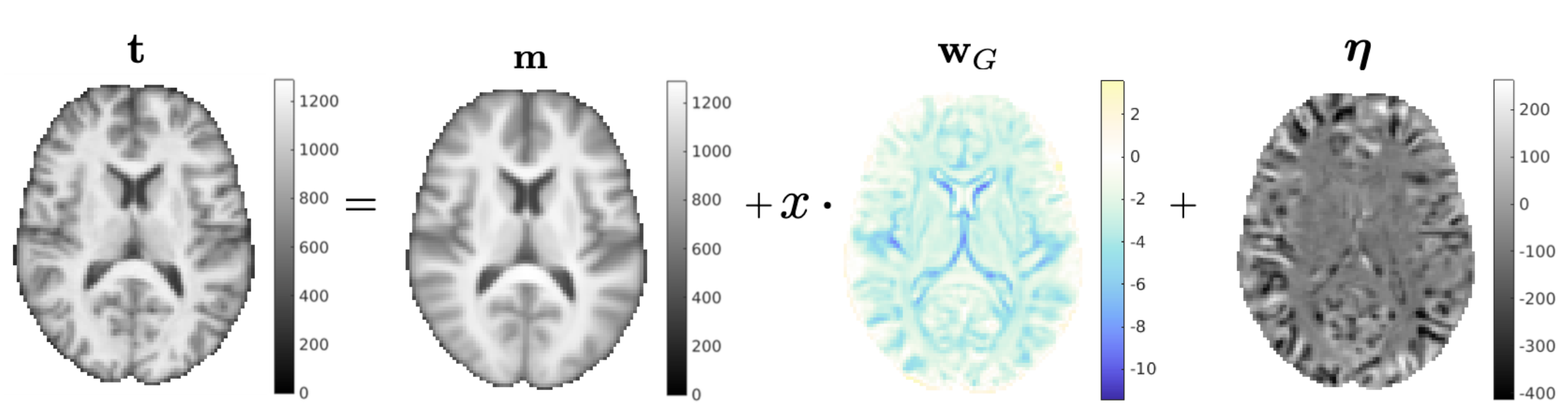
Figure 1: Example of the forward model (1), applied to modeling the effect of age on brain morphology. Here $x$ denotes the difference between the age of the subject and the average age in a training set.

3.2 Making predictions

When the parameters of the model ($\mathbf{W}$ and $\mathbf{C}$) are known, the unknown target variable $x^{*}$ of a subject with image $\mathbf{t}^{*}$ can be inferred by inverting the model using Bayes’ rule. For a binary target variable $x^{*}\in\{0,1\}$, it is well-known that the target posterior distribution takes the form of a logistic regression classifier (Hart et al., 2000): Assuming the two outcomes have equal prior probability, we obtain (cf.  A)

$$p(x^{*}=1|\mathbf{t}^{*},\mathbf{W},\mathbf{C})=\sigma\big{(}\mathbf{w}_{D}^{T}\mathbf{t}^{*}+w_{o}\big{)},$$ (2)

where

$$\mathbf{w}_{D}=\mathbf{C}^{-1}\mathbf{w}_{G}$$ (3)

are a set discriminative spatial weights, $\sigma(a)=1/(1+e^{-a})$ denotes the logistic function, and $w_{o}=-\mathbf{w}_{D}^{T}(\mathbf{m}+\mathbf{w}_{G}/2)$. The maximum a posteriori (MAP) estimate of $x^{*}$ is therefore $1$ if

$$\mathbf{w}_{D}^{T}\mathbf{t}^{*}+w_{o}>0,$$ (4)

and $0$ otherwise.

For a continuous target variable with a flat prior $p(x^{*})\propto 1$, the posterior distribution is Gaussian with variance

$$v=\left(\mathbf{w}_{G}^{T}\mathbf{C}^{-1}\mathbf{w}_{G}\right)^{-1}$$ (5)

and mean

$$\tilde{x}^{*}=v(\mathbf{w}_{D}^{T}\mathbf{t}^{*}+b_{0}),$$ (6)

where $b_{0}=-\mathbf{w}_{D}^{T}\mathbf{m}$ (cf. A). The predicted value of $x^{*}$ is therefore given by (6), which again involves taking the inner product of the discriminative weights $\mathbf{w}_{D}$ with $\mathbf{t}^{*}$. An example of model inversion in case of age prediction is shown in Fig. 2.

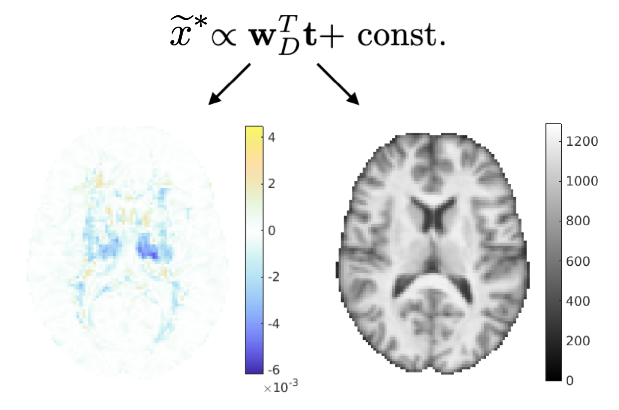
Figure 2: Illustration of how a subject’s age is estimated by inverting the model shown in Fig. 1.

3.3 Model training

In practice the model parameters $\mathbf{W}$ and $\mathbf{C}$ need to be estimated from training data. Given $N$ training pairs $\{\mathbf{t}_{n},x_{n}\}_{n=1}^{N}$, their maximum likelihood (ML) estimate is obtained by maximizing the marginal likelihood

$$p\left(\{\mathbf{t}_{n}\}_{n=1}^{N}|\{x_{n}\}_{n=1}^{N},\mathbf{W},\mathbf{C}\right)=\prod_{n=1}^{N}\mathcal{N}\left(\mathbf{t}_{n}|~{}\mathbf{W}\boldsymbol{\phi}_{n},\mathbf{C}\right)$$ (7)

with respect to $\mathbf{W}$ and $\mathbf{C}$, where we have defined $\boldsymbol{\phi}_{n}=(1,x_{n})^{T}$. For the spatial maps, the solution is given in closed form (cf.  B):

$$\mathbf{W}=\left(\sum_{n=1}^{N}\mathbf{t}_{n}\boldsymbol{\phi}_{n}^{T}\right)\left(\sum_{n=1}^{N}\boldsymbol{\phi}_{n}\boldsymbol{\phi}_{n}^{T}\right)^{-1}.$$ (8)

However, obtaining the noise covariance matrix $\mathbf{C}$ directly by ML estimation is problematic: $\mathbf{C}$ has $J(J+1)/2$ free parameters, which is orders of magnitude more than there are training samples (recall that $J$ is the number of voxels). To be able to control the number of parameters while still capturing the dominant correlations in the noise, we impose a specific structure on $\mathbf{C}$ by using a latent variable model known as factor analysis (Bishop, 2006). In particular, we model the noise as

$$\boldsymbol{\eta}=\mathbf{V}\mathbf{z}+\boldsymbol{\epsilon},$$ (9)

where $\mathbf{z}$ is a small set of $K$ unknown latent variables distributed as $p(\mathbf{z})=\mathcal{N}(\mathbf{z}|\mathbf{0},\mathbb{I}_{K})$, $\mathbf{V}$ contains $K$ corresponding, unknown spatial weight maps, and $\boldsymbol{\epsilon}$ is a zero-mean Gaussian distributed error with unknown diagonal covariance $\boldsymbol{\Delta}$. Marginalizing over $\mathbf{z}$ yields a zero-mean Gaussian noise model (Bishop, 2006) with covariance matrix

$$\mathbf{C}=\mathbf{V}\mathbf{V}^{T}+\boldsymbol{\Delta},$$

which is now controlled by a reduced set of parameters $\mathbf{V}$ and $\boldsymbol{\Delta}$. The number of columns in $\mathbf{V}$ (i.e., the number of latent variables $K$) is a hyperparameter in the model that needs to be tuned experimentally.

Plugging in the ML estimate of $\mathbf{W}$ given by (8), the parameters $\mathbf{V}$ and $\boldsymbol{\Delta}$ maximizing the marginal likelihood (7) can be estimated using an Expectation-Maximization (EM) algorithm (Rubin and Thayer, 1982). Defining

$$\boldsymbol{\eta}_{n}=\mathbf{t}_{n}-\mathbf{W}\boldsymbol{\phi}_{n}$$ (10)

as the noise vector of training subject $n$, this yields an iterative algorithm that repeatedly evaluates the posterior distribution over the latent variables:

$$p(\mathbf{z}_{n}|\boldsymbol{\eta}_{n},\mathbf{V},\boldsymbol{\Delta})=\mathcal{N}(\mathbf{z}_{n}|\boldsymbol{\mu}_{n},\boldsymbol{\Sigma}),\quad\forall n$$ (11)

where $\boldsymbol{\mu}_{n}=\boldsymbol{\Sigma}\mathbf{V}^{T}\boldsymbol{\Delta}^{-1}\boldsymbol{\eta}_{n}$ and $\boldsymbol{\Sigma}=(\mathbb{I}_{K}+\mathbf{V}^{T}\boldsymbol{\Delta}^{-1}\mathbf{V})^{-1}$, and subsequently updates the parameters accordingly:

$$\mathbf{V}\leftarrow\left(\sum_{n=1}^{N}\boldsymbol{\eta}_{n}\boldsymbol{\mu}_{n}^{T}\right)\left(\sum_{n=1}^{N}\left(\boldsymbol{\mu}_{n}\boldsymbol{\mu}_{n}^{T}+\boldsymbol{\Sigma}\right)\right)^{-1}$$ (12)

$$\boldsymbol{\Delta}\leftarrow\mathrm{diag}\left(\frac{1}{N}\sum_{n=1}^{N}\boldsymbol{\eta}_{n}\boldsymbol{\eta}_{n}^{T}-\mathbf{V}\frac{1}{N}\sum_{n=1}^{N}\boldsymbol{\mu}_{n}\boldsymbol{\eta}_{n}^{T}\right).$$ (13)

Here $\mathrm{diag}(\cdot)$ sets all the non-diagonal entries to zero.

3.4 Practical implementation

The method outlined above involves manipulating matrices of size $J\!\times\!J$. Despite the high dimensionality (recall that $J$ is the number of voxels), computations can be performed efficiently by exploiting the structure of these matrices: As detailed in  C, both training and predicting can be implemented in a way that only involves the posterior covariance of the latent variables $\boldsymbol{\Sigma}$, which is of much smaller size $K\!\times\!K$.

In our implementation, we center the target variable $x$, i.e., we use values from which the sample mean in the training set has been subtracted. As shown in D, this has the advantage that the estimated template $\mathbf{m}$ then represents the anatomy of the “average” subject in the training set, i.e., $\mathbf{m}=1/N\sum_{n=1}^{N}\mathbf{t}_{n}$. For estimating the parameters $\boldsymbol{V}$ and $\boldsymbol{\Delta}$ of the noise model, we first perform a voxel-wise rescaling of the noise vectors $\{\boldsymbol{\eta}_{n}\}_{n=1}^{N}$, such that each voxel has unit variance across the training subjects. We then initialize the EM algorithm by using a matrix with standard Gaussian random entries for $\mathbf{V}$, and the identity matrix for $\boldsymbol{\Delta}$. Convergence of the EM procedure is detected when the relative change in the log marginal likelihood drops below $10^{-5}$ between iterations. The elements in the estimated $\mathbf{V}$ and $\boldsymbol{\Delta}$ are then rescaled back to the original intensity space to obtain the final parameters of the noise model.

The code for the proposed model is available at https://github.com/chiara-mauri/Interpretable-subject-level-prediction, with both Matlab and Python implementations.

4 Experiments on Age and Gender Prediction

In this section, we present experiments on the task of predicting a subject’s age and gender from their brain MRI scan. Specifically, we compare the behavior of the proposed method with that of three state-of-the-art benchmark methods, when the size of the training set is varied.

4.1 Experimental set-up

The benchmarks we used consist of a nonlinear-discriminative (SFCN (Peng et al., 2021)), a linear-discriminative (RVoxM (Sabuncu and Van Leemput, 2012)), and a nonlinear-generative (VAE (Zhao et al., 2019)) method for image-based prediction. Together with the proposed method, which is linear-generative in the basic form analyzed here, these benchmarks form a representative sample of the spectrum of methods available to date.

We trained each of these methods on randomly sampled subsets of 26,127 T1-weighted scans of healthy subjects drawn from the UK Biobank (Alfaro-Almagro et al., 2018). Each of these subjects was between 44 and 82 years old, and was scanned on one of three identical 3T scanners using the same MRI protocol. In our experiments, we used the skull-stripped and bias-field corrected T1-weighted scans that are made publicly available, which are computed using a nonlinear registration with the MNI152 template (see (Alfaro-Almagro et al., 2018) for details). We took advantage of these nonlinear registrations to warp and resample all the scans to the same MNI152 template space using linear interpolation. The resulting 1mm isotropic T1-weighted images then formed the input of the various image-prediction algorithms.

To analyze the behavior of the different methods when the training set size is gradually increased from $100$ to almost $10,000$ subjects, we trained each method multiple times for each training set size. Specifically, each training run was repeated 10 times, with different randomly sampled training subjects, except for the larger training sizes ($N\!>\!1,000$) where the number of repetitions was limited to 3 to reduce the computational burden. After training, the prediction performance of each model was evaluated on a fixed set of $1,000$ randomly sampled test subjects not overlapping with the training subjects. For the age prediction task, the Mean Absolute Error (MAE)  was used as the evaluation criterion, whereas the average classification accuracy was used in the gender prediction experiments.

Similar to the experimental set-up of (Peng et al., 2021), we also had a separate, fixed validation set of $500$ randomly sampled subjects. This was used to tweak one or two hyperparameters for each method (see details below), using a grid search to optimize MAE (for age) and classification accuracy (for gender) for each training run.

4.2 Implementation of the benchmark methods

The four methods under comparison were implemented as follows:

• Proposed method: We performed all the experiments with the proposed method in Matlab, running on a Linux CPU machine (Intel Xeon E5-2660V3 10 Core CPU 2.60GHz, 128GB RAM). To speed up computations, the number of voxels was reduced by masking out the background (by thresholding the average of all images in each training set), and by downsampling the input data to a 3mm isotropic resolution. This downsampling was found not to affect the prediction performance in pilot experiments. For each training run, performance on the validation set was used to set the number of latent variables $K$, which is the only hyperparameter of the method. An example of a model trained this way is shown in Figs. 3, 4 and 5.

• RVoxM: This is a discriminative method that imposes sparsity and spatial smoothness on its weight map as a form of regularization (Sabuncu and Van Leemput, 2012). We used the Matlab code that is publicly available, with some adaptations to make it more efficient (by parallelizing part of the training loop) and, for gender prediction, more robust to high-dimensional input. The same background masking, downsampling procedure and computer hardware was used as for the proposed method in the experiments. The method has a single hyperparameter to control the spatial smoothness of the weight map that it computes, which was tuned on the validation set for each training run.

• SFCN: This is the lightweight convolutional neural network proposed by (Peng et al., 2021), who, to the best of our knowledge, have reported the best performance for brain age prediction to date. Since code for training this method is not publicly available, we modified the implementation of (Mouches et al., 2022) to match the description provided in (Peng et al., 2021) as closely as possible. In particular, we replicated the same data augmentation scheme, network architecture, L2 weight decay and batch size, deviating only in the last network layer as discretizing age into 40 bins (as described in (Peng et al., 2021)) did not benefit prediction accuracy in our experiments. The method directly takes 1mm isotropic images as input, and was therefore run on a high-end GPU with a sufficiently large amount of memory (NVIDIA A100 SXM4 GPU with 40 GB of RAM) in our experiments. For each training run, the validation set was used to determine the optimal number of training epochs of this method.

• VAE: This is a generative method for age prediction (Zhao et al., 2019) with publicly available training code. It can be regarded as a generalization of the proposed method, where the latent variables are expanded nonlinearly through a deep neural network, which precludes exact model inversions and makes computations more involved. Since the method is designed to work with images that are downsampled to 2mm isotropic resolution and cropped around the ventricles (Zhao et al., 2019), the comparison with this method was performed separately from the other two benchmarks, with both the VAE and the proposed method running on the same cropped 2mm volumes. Furthermore, since the number of latent variables is hardcoded to 12 in the implementation, we tested only training sizes in a similar range (from 100 to 400 training subjects) as the one used in the paper (196 subjects). For the experiments, we ran the VAE on a NVIDIA GeForce RTX 2080 Ti GPU with 11 GB of RAM. The method contains two regularization hyperparameters (dropout factor and L2 regularization), which were tuned on the validation set for each training run.

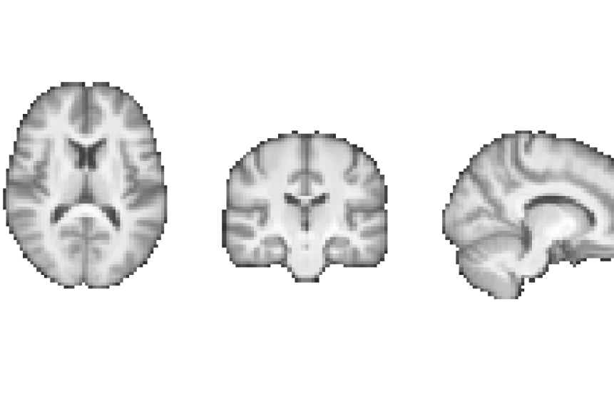
Figure 3: The estimated template $\mathbf{m}$ (the average image in the training set) when the model is trained on $N=2,600$ subjects in an age prediction task.

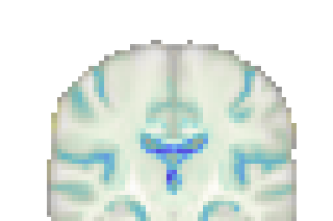
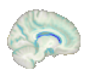
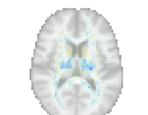
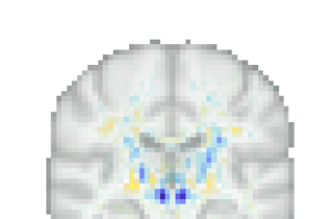
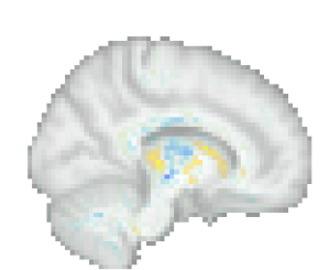
Figure 4: Top: the generative map $\mathbf{w}_{G}$ – expressing the effect of aging – estimated from $N=2,600$ subjects, overlaid on the template of Fig. 3. Voxels with zero weight are transparent. Bottom: the corresponding discriminative map $\mathbf{w}_{D}$ that is used for making age predictions. The discrepancy between these two maps is analyzed in Sec. 4.5.

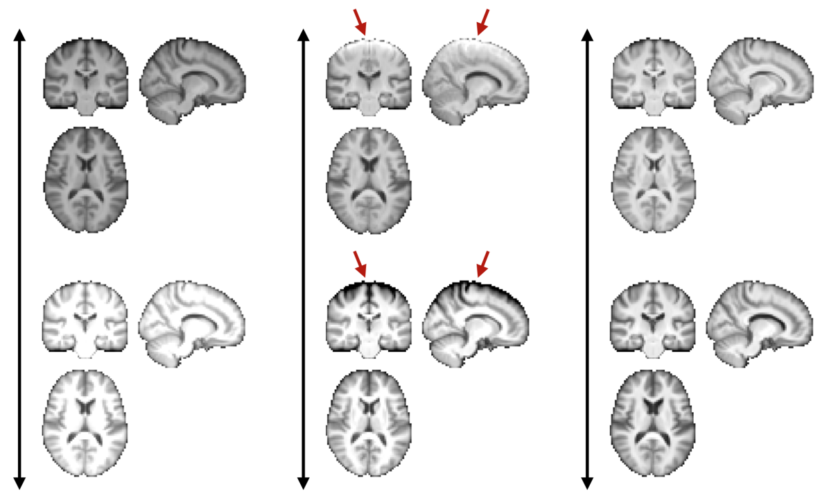
$1^{st}$ mode of variation

$2^{nd}$ mode of variation

$3^{rd}$ mode of variation

Figure 5: Illustration of the major modes of variation captured by the linear-Gaussian noise model, when trained on $N=2,600$ subjects in an age prediction task. Each mode illustrates the effect of applying one of the three first eigenvectors of $\mathbf{V}\mathbf{V}^{T}$ (the component of $\mathbf{C}$ that has spatial structure) on the template of Fig. 3. The top and bottom figures show the template modified in the positive and negative direction of the eigenvectors, respectively. Note that the first eigenvector seems to encode a general brightening/darkening of the image intensities, while the second one models residual bias fields that were not removed in the preprocessing of the UK Biobank data.

4.3 Prediction performance and training times

Fig. 6 shows the prediction performance of the proposed method, RVoxM and SFCN as the number of training subjects is varied, both for predicting age (Fig. 6 left) and gender (Fig. 6 right). As expected, all prediction performances improve as the training size increases. In the age prediction task, the proposed method yields generally the best performance when the training set size is up to 2,600 subjects, after which SFCN is the better method. For gender prediction, SFCN is clearly outperformed by both RVoxM and the proposed method.

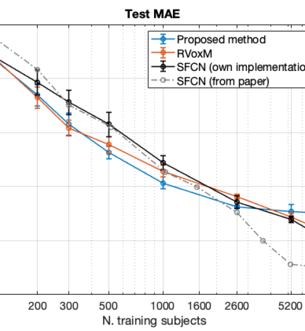
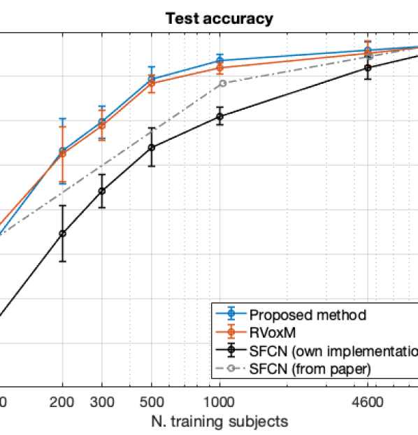
Figure 6: Prediction performance of the proposed method, RVoxM and SFCN for age (left) and gender (right) as the number of training subjects is varied. For each method, the full line shows the average performance across multiple training runs, and the whiskers extend to one standard deviation away from the average. The test MAE for age is indicated in years. For reference, we also include the performance of SFCN as reported in (Peng et al., 2021), although the results are not entirely comparable.

For completeness, Fig. 6 also includes the results for SFCN as reported by its authors in (Peng et al., 2021), where a similar experimental set-up as ours was used. It can be seen that, although our implementation closely followed the description provided by the authors, we were not always able to match their reported performance: Especially for gender prediction, and for age prediction with very large training sets, there are considerable discrepancies between the two implementations. One possible explanation is that SFCN is a complex model with many more “knobs” to be tuned correctly than the proposed method, which has only a single hyperparameter. Another explanation is that the experimental set-up is not entirely comparable: In (Peng et al., 2021) the model is only trained on one training set for each training size; the subjects in their test set are different from ours; and they used affinely instead of nonlinearly registered scans (although the latter point is reported to yield only minimal differences in (Peng et al., 2021), which we can confirm based on our own experiments).

Table 1 reports, for the age prediction experiment, the training times required by the proposed method, RVoxM and SFCN. SFCN is by far the slowest to train, requiring many hours even for very small training sizes, and several days for large ones. Up to training sizes of 1,000 subjects, the proposed method is considerably faster to train than RVoxM (dozens of minutes CPU time at most), but slows down for larger training sizes. This can be explained by the fact that the optimal number of latent variables in our model (hyperparameter $K$) increases rapidly with the number of training subjects, as shown in Table 2. When interpreting the training times of RVoxM and the proposed method on the one hand, and those of SFCN on the other, it should be taken into account that the latter uses hardware acceleration but also works with much larger (non-downsampled) input volumes.

	N=100	N=200	N=300	N=500	N=1,000	N=2,600	N=5,200	N=7,800
Proposed method	1.20 min	0.67 min	1.94 min	9.53 min	32 min	$\approx$3h	$\approx$15h	$\approx$ 69 h
RVoxM	92 min	66 min	75 min	76 min	129 min	127 min	$\approx$ 22 h	$\approx$ 21 h
SFCN	$\approx$ 8h	$\approx$ 11 h	$\approx$ 16 h	$\approx$ 18 h	$\approx$ 34h	$\approx$ 76h	$\approx$ 69h	$\approx$ 102 h

Table 1: Training times in the age prediction task for the proposed method, RVoxM and SFCN. These training times were evaluated at the optimal value of a single hyperparameter for each method, determined on an external validation set. The reported times are the average across all training runs for each training set size $N$.

	N=100	N=200	N=300	N=500	N=1,000	N=2,600	N=5,200	N=7,800
$K$	20	21	52	86	120	367	1,833	3,333

Table 2: Optimal number of latent variables $K$ of the proposed method when predicting age, as determined on an external validation set. The reported number is the rounded average across all training runs for each training set size $N$.

Finally, Fig. 7 shows the age prediction performance of the VAE and the proposed method, as a function of the training set size. The proposed method achieves better results for every training size tested. This suggests that, at least when only a few hundred subjects are available for training, adding nonlinearities in the method’s noise model is not beneficial. Furthermore, the VAE is considerably slower to train than the proposed method: around 10 min GPU time for 200 training subjects, vs. 1 min CPU time with the proposed method.

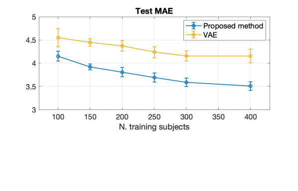
Figure 7: Age prediction performance of the VAE and the proposed method, when applied to 2mm isotropic images cropped around the ventricles, represented in the same way as in Fig. 6.

4.4 Bias-variance trade-off

More insight into the prediction performances reported in the previous section can be obtained using the so-called bias-variance decomposition. Specifically for age, which is a continuous variable, a particular method’s mean squared error (MSE) can be decomposed as follows (Bishop, 2006):

$$\underbrace{\mathbb{E}_{D}\left[\left(x^{*}-\tilde{x}^{*}_{D}\right)^{2}\right]}_{MSE}=\underbrace{\left(x^{*}-\mathbb{E}_{D}\left[\tilde{x}^{*}_{D}\right]\right)^{2}}_{bias^{2}}+\\ +\underbrace{\mathbb{E}_{D}\left[\left(\tilde{x}^{*}_{D}-\mathbb{E}_{D}\left[\tilde{x}^{*}_{D}\right]\right)^{2}\right]}_{variance}.$$ (14)

Here $x^{*}$ denotes the real age of a given test subject, $\tilde{x}^{*}_{D}$ is the predicted age when the method is trained on a particular dataset $D$ of a certain size, and $\mathbb{E}_{D}[\cdot]$ denotes the average over multiple such training sets. In our set-up, in which each method is trained multiple times using different randomly sampled subjects, the bias component in (14) reflects a systematic error that is persistent across the training runs, whereas the variance component indicates how much the predictions change between the different training runs  (Hart et al., 2000; Bishop, 2006; Domingos and Pazzani, 1997). Typically, flexible models tend to have low bias but high variance, reflecting an overfitting to the training data, while strongly constrained methods display the opposite behavior, resulting in underfitting of the training data (Hart et al., 2000; Bishop, 2006; Domingos and Pazzani, 1997).

Fig. 8 (left) shows how the bias, the variance and the resulting MSE change in the age prediction experiment, when the training set size is varied. The various curves were obtained by averaging (14) across all test subjects for our method (blue), RVoXM (red) and SFCN (black). The proposed method generally has the highest bias among the three methods; however this is off-set by a lower variance, resulting in a strong overall prediction performance in training set sizes of up to 2,600 subjects. Its low variance is obtained by controlling the flexibility of the method: when the number of training subjects is small, only a limited number of latent variables is selected (see Table 2), resulting in a simple, highly regularized model that successfully avoids overfitting to the training data. As the training size increases, the number of latent variables is allowed to grow, resulting in gradually more flexible models with decreased bias and therefore better prediction performance (see Fig. 8 (left)). However, for very large training sets (over 2,600 subjects), the method’s strong modeling assumptions prevent it from decreasing its bias further, and the nonlinear SFCN can now take advantage of its flexibility (lower bias) without overfitting (variance comparable to the proposed method), resulting in a better prediction performance.

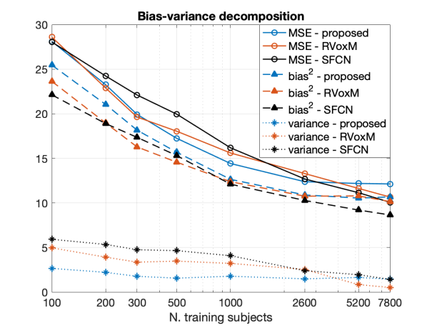
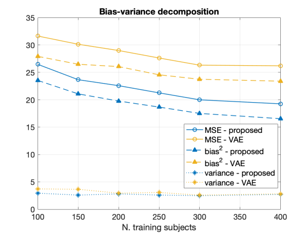
Figure 8: Left: bias-variance decomposition for the age prediction results shown in Fig. 6 (left). Right: the same for the results shown in Fig. 7.

Fig. 8 (right) shows the results of the bias-variance decomposition for the VAE and our method, when applied to age prediction from 2mm croppped data. It can be seen that the VAE’s lower prediction performance (reported in Sec. 4.3) can be attributed to its significantly higher bias, presumably due to the variational approximations (Kingma and Welling, 2013) that are used to invert its model.

4.5 Interpretability analysis

A key advantage of the proposed method over discriminative methods such as RVoxM and SFCN is that, in addition to the discriminative map $\mathbf{w}_{D}$ that it uses to make predictions, it also computes a generative map $\mathbf{w}_{G}$ that expresses the causal effect of the variable of interest on brain morphology. To illustrate why this is important, Fig. 9 shows, for three different training set sizes, the discriminative map $\mathbf{w}_{D}$ computed by our method for predicting age, along with the corresponding discriminative map of RVoXM and the SmoothGrad saliency map (Smilkov et al., 2017) – a generalization of linear spatial maps to nonlinear methods (Adebayo et al., 2018) – of SFCN. The inconsistencies of these maps across both the training set sizes and the different methods, and their overall lack of correspondence with the known neurobiology of aging, illustrate the difficulty of using discriminative maps for human interpretation.

More insight can be gained by examining the proposed method specifically, since it uses disciminative maps that are derived from generative ones. It is worth noting that estimating the generative maps from training data is itself quite stable, since it merely amounts to fitting two basis functions to hundreds of measurements in each voxel (cf. (8)). Furthermore, as illustrated in Fig. 10, the resulting maps are intuitive to interpret, since they show typical age-related effects such as cortical thinning and ventricle enlargement (Fjell et al., 2009; Fjell and Walhovd, 2010). When the discriminative maps are subsequently computed as $\mathbf{w}_{D}=\mathbf{C}^{-1}\mathbf{w}_{G}$, however, a strong dependency on the training set size is introduced, because the method explicitly controls the complexity of its noise model $\mathbf{C}$ in response to the size of the available training set (the bias-variance trade-off of Sec. 4.4). $\mathbf{C}$ can also capture peculiarities in the data that may be relevant for improving prediction performance, but not for human interpretation. An example of this was shown in Fig. 5, where overall brightness variations and residual MR bias field artifacts were picked up by the noise model. Through $\mathbf{C}$, such noise patterns can find their way into $\mathbf{w}_{D}$, producing hard-to-interpret spatial maps that no longer reflect the expected age-related brain atrophy patterns. This is clearly illustrated in Fig. 4, where the discriminative map $\mathbf{w}_{D}$ is contrasted with the corresponding generative map $\mathbf{w}_{G}$.

The reason the noise covariance $\mathbf{C}$ is taken into account in $\mathbf{w}_{D}$ – which in turn makes $\mathbf{w}_{D}$ hard to interpret – can be illustrated with a simple toy example involving only two “voxels”, shown in Fig. 11. When the method is tasked with computing the prediction $\tilde{x}^{*}$ from an image $\mathbf{t}^{*}$, it effectively decomposes $\mathbf{t}^{*}$ into its most likely constituent components: $\mathbf{m}$ (a population template), $\tilde{x}^{*}\mathbf{w}_{G}$ (the estimated causal effect), and $\tilde{\boldsymbol{\eta}}^{*}$ (the most likely noise vector) – cf. (1) and Fig. 1. In this process, parts of the signal that are well-explained by the noise model $\mathbf{C}$ can be attributed to the noise component $\tilde{\boldsymbol{\eta}}^{*}$, and therefore effectively discarded when estimating $\tilde{x}^{*}$. This is illustrated in Fig. 11 (middle). Mathematically, the same value $\tilde{x}^{*}$ can also be obtained by simply computing the inner product $\mathbf{w}_{D}^{T}\mathbf{t}^{*}$ (cf. (6) and Fig. 2), which folds the process of separating the effect of interest from noise patterns into a single operation. This amounts to projecting the given data point $\mathbf{t}^{*}$ orthogonally onto the direction $\mathbf{w}_{D}$, as illustrated in Fig. 11 (right). However, this projection operation is hard to interpret on its own: $\mathbf{w}_{D}$ only reveals the final recipe of how predictions are computed, but no longer the underlying logic.

In addition to visualizing its generative maps directly for human interpretation, the causal interpretation of our model can also be used to simulate the effect of aging on actual images. On the population level, this can be achieved by computing age-specific templates $\mathbf{m}+x\mathbf{w}_{G}$ for different values of $x$, as illustrated in Fig. 12. More detailed explanations can also be provided at the level of the individual subject, using counterfactuals (Pearl and Mackenzie, 2018) – imaginary images of specific individuals if they had been younger or older. Given an image $\mathbf{t}$ and the real age $x$, (10) can be used to compute the subject-specific noise vector $\boldsymbol{\eta}$, which captures the subject’s individual idiosyncrasies that are not explained by the population-level causal model. Counterfactual images can then be obtained by re-assembling the forward model from its constituent components, using a different, imaginary age $x$ in (1). Examples of this process are shown in Fig. 13.

	$\mathbf{N=300}$	$\mathbf{N=2,600}$	$\mathbf{N=7,800}$
Proposed ($\mathbf{w}_{D}$)
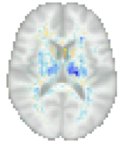
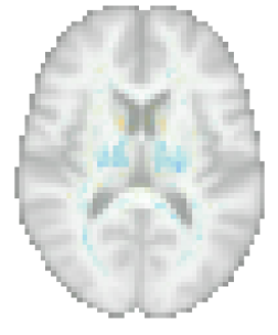
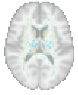
RVoxM
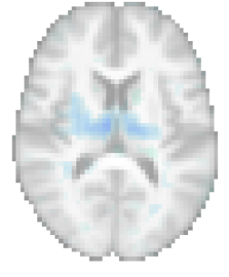
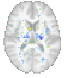
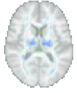
SFCN

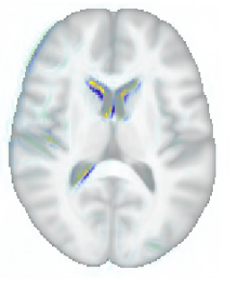
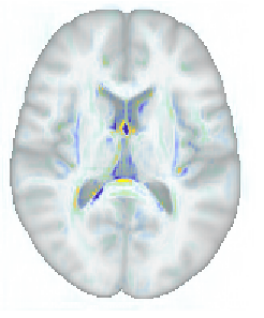
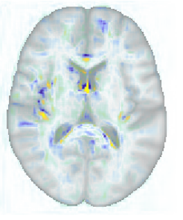
Figure 9: Discriminative maps of proposed method, RVoxM, and SFCN (with SmoothGrad) obtained for age prediction with varying training set sizes, overlaid on a template. Voxels with zero weight are transparent. Since SmoothGrad yields subject-specific maps, we averaged across all test subjects to obtain population-level maps for SFCN.

$\mathbf{N=300}$	$\mathbf{N=2,600}$	$\mathbf{N=7,800}$

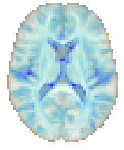
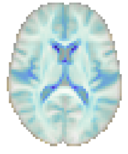
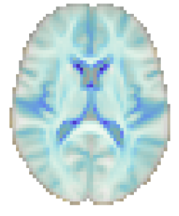
Figure 10: Generative maps $\mathbf{w}_{G}$ computed by the proposed method for age prediction, for different training set sizes. In addition to expressing known aging patterns in the brain, these maps also show consistency across the different training sizes.

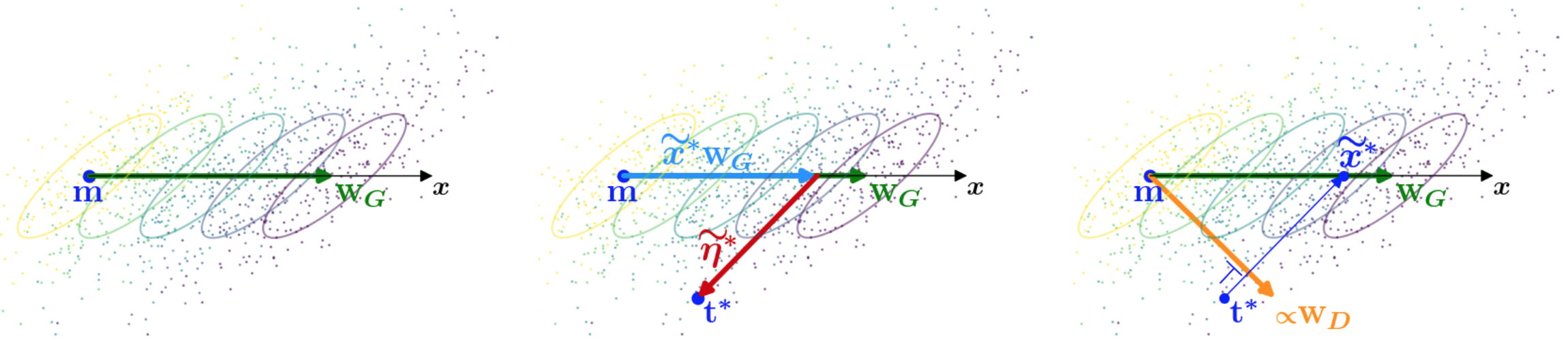
Figure 11: Left: illustration of a the image generation process in a toy example. The figure shows the template $\mathbf{m}$, the generative map $\mathbf{w}_{G}$, and contour plots of the noise covariance matrix $\mathbf{C}$. Also shown are randomly generated 2D data points (dots in the figure), corresponding to 5 discrete values of a continuous variable of interest $x$ (marked with different colors). The discretization was performed for visualization purposes. Middle: when the model is inverted to compute a predicted value $\tilde{x}^{*}$ for a given data point $\mathbf{t}^{*}$ , the signal is effectively decomposed into $\mathbf{t}^{*}=\mathbf{m}+\tilde{x}^{*}\mathbf{w}_{G}+\tilde{\boldsymbol{\eta}}^{*}$. Right: the same result $\tilde{x}^{*}$ can also be obtained by projecting the data point $\mathbf{t}^{*}$ orthogonally onto the direction $\mathbf{w}_{D}=\mathbf{C}^{-1}\mathbf{w}_{G}$. This operation is mathematically equivalent to decomposing the signal into its components as in the middle figure, but not in terms of interpretability, since causal effect and noise pattern are intermingled in $\mathbf{w}_{D}$.

47 years	64 years	80 years

Figure 12: Age-specific templates generated by the proposed method trained on $N=2,600$ subjects, representing the expected “average” image for a specific age. Known age-related effects, such as wider sulci and bigger ventricles (Fjell et al., 2009; Fjell and Walhovd, 2010), are clearly displayed.

47 years (real)	80 years (counterfactual)	80 years (real)	47 years (counterfactual)

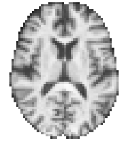
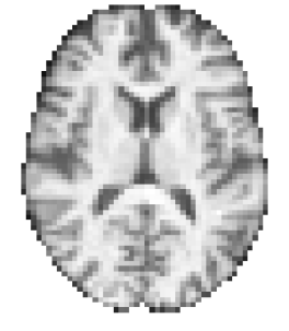
Figure 13: Two examples of counterfactuals generated by the model for age prediction, trained on $N=2,600$ subjects. Left: real and counterfactual image of a 47-year old subject who is artificially aged to 80 years. Right: the same for a 80-year old subject who is rejuvenated to age 47.

5 Extensions

Here we show how the method can be further extended to take into account additional subject-specific covariates, as well as nonlinear dependencies on the variable of interest.

5.1 Additional covariates

When additional demographic or clinical information is available about the subjects, it is straightforward to include this in the model. This can be useful for further improving prediction accuracy, as demonstrated below, or for removing the effect of confounders that would otherwise invalidate the causal interpretation of the generative maps (see Sec. 6).

Assuming each subject has $L$ extra variables $y^{1},\ldots,y^{L}$, the model (1) can be extended to

$$\mathbf{t}=\mathbf{m}+x\mathbf{w}_{G}+\sum_{l=1}^{L}y^{l}\mathbf{w}_{y}^{l}+\boldsymbol{\eta},$$

where $\mathbf{w}_{y}^{1},\ldots,\mathbf{w}_{y}^{L}$ are now extra spatial weight maps that also need to be estimated. During training, the corresponding parameters $\mathbf{W}=(\mathbf{m},\mathbf{w}_{G},\mathbf{w}_{y}^{1},\ldots,\mathbf{w}_{y}^{L})$, $\mathbf{V}$ and $\boldsymbol{\Delta}$ can still be estimated using (8), (12) and (13), provided that $\boldsymbol{\phi}_{n}=(1,x_{n},y_{n}^{1},\ldots,y_{n}^{L})^{T}$ is used instead of $\boldsymbol{\phi}_{n}=(1,x_{n})^{T}$. To predict an unknown variable of interest $x^{*}$ from a subject with image $\mathbf{t}^{*}$ and covariates $y^{*1},\ldots,y^{*L}$, (4) and (6) remain valid when $\mathbf{t}^{*}$ is replaced by $\left(\mathbf{t}^{*}-\sum_{l}y^{*l}\mathbf{w}_{y}^{l}\right)$.

To test this model extension, we considered a classification experiment of multiple sclerosis (MS) patients vs. healthy controls, using both age and gender as additional covariates. For this experiment, we used a private dataset from Klinikum rechts der Isar (Munich, Germany) consisting of lesion-filled T1-weighted scans of 131 MS subjects and 131 age- and gender-matched controls. As input to the method we used probabilistic gray matter segmentations computed with SPM12, after warping them to standard space and modulating them (Ashburner et al., 2014) to preserve signal that would otherwise be removed by the spatial normalization.

In order to check whether the use of the extended model (with age and gender included as covariates) improves classification accuracy compared to the baseline method, we treated the inclusion of the covariates in the model as an extra binary hyperparameter in our experiments, determined in the same way as the other hyperparameter $K$ of the method. Given the limited number of subjects in the dataset, this was implemented within a nested 5-fold cross-validation (CV) setting: For each data split of the outer CV loop into a training and a test set, an additional CV was performed multiple times on the training set, evaluating different values of the two hyperparameters. The optimal hyperparameters were then selected and used to re-train the model on the entire training set, which was then evaluated on the test set. This procedure was repeated for each data split in the outer loop, to yield overall prediction performances.

In our experiments, the model with age and gender included as covariates was selected in all the CV folds, and yielded better prediction performance on the test data compared to the baseline model (classification accuracy of 0.72 vs. 0.70).

5.2 Nonlinearities in the causal model

Another extension of (1) is to consider nonlinear cause-effect relations in the model:

$$\mathbf{t}=\mathbf{m}+x\mathbf{w}_{G}+\sum_{l=1}^{L}f_{l}(x)\mathbf{w}_{y}^{l}+\boldsymbol{\eta},$$

where each $f_{l}(x)$ is some nonlinear function of the (continuous) variable of interest $x$. During training, this can be viewed as merely a special case of the model extension of Sec. 5.1: the mappings $f_{l}(\cdot),\,\,l=1,\ldots,L$ can be evaluated for each training subject, and treated as known additional covariates in the model. Predicting with a trained model is no longer governed by the linear equation (6), though. We therefore invert the model by finely discretizing $x^{*}$ into $P$ distinct values $x_{p},p=1,\ldots,P$, and evaluating the posterior probability of each. Assuming a flat prior, this yields

$$p(x^{*}=x_{p}|\mathbf{t}^{*},\mathbf{W},\mathbf{C})=\frac{\gamma_{p}}{\sum_{p^{\prime}=1}^{P}\gamma_{p^{\prime}}},$$

where $\gamma_{p}=\mathcal{N}(\mathbf{t}|\mathbf{m}+x_{p}\mathbf{w}_{G}+\sum_{l=1}^{L}f_{l}(x_{p})\mathbf{w}_{y}^{l},\mathbf{C})$ can be evaluated efficiently using (17), (18) and (19). Predictions are then obtained as the expected value of this posterior distribution:

$$\tilde{x}^{*}=\sum_{p=1}^{P}x_{p}p(x^{*}=x_{p}|\mathbf{t}^{*},\mathbf{W},\mathbf{C}).$$

In order to demonstrate this extension, we tested whether the inclusion of an extra quadratic term in the forward model (i.e., $f_{1}(x)=x^{2}$) can improve age estimation results compared to the basic, linear model. For this purpose, we used modulated gray matter segmentations (computed in the same way as described in Sec. 5.1) of T1-weighted scans of 562 healthy subjects from the IXI dataset. This dataset was selected because aging has been shown to have an approximately quadratic effect across adulthood on some brain structures (Walhovd et al., 2005), and the IXI dataset covers an age span that is large enough (20-86 years) to possibly exploit this behaviour for prediction purposes.

We used a similar set-up as the one described in Sec. 5.1, where the possible inclusion of the quadratic term in the model is considered an additional binary hyperparameter in a nested 5-fold cross-validation setting. For the discretization, we used $P=20$ intervals covering the entire age range. Using this set-up, we found that the quadratic model was selected in all the CV folds, and yielded smaller age prediction test errors than the baseline method (MAE of 4.36 vs. 4.73 years).

6 Discussion and Conclusion

In this paper, we have proposed a lightweight method for image-based prediction that is inherently interpretable. It is based on classical human brain mapping techniques, but includes a multivariate noise model that yields accurate subject-level predictions when inverted. Despite its simplicity, the method predicts well in comparison with state-of-the art benchmarks, especially in typical training scenarios (those with no more than a few thousand training subjects) where more flexible techniques become prone to overftting.

Throughout the paper we have stressed the causal interpretation of the data generating process in our models, and used that as a basis for explaining the method’s predictions in ways that are anatomically meaningful. Such causal interpretations, however, are only valid if the underlying modeling assumptions are sufficiently correct. Beyond mere technical aspects such as assumptions of linearity, more fundamental model violations could also include the sheer direction of causality: While we can be fairly certain that such factors as age, gender and disease status affect how the brain looks like, in other cases (e.g., when predicting clinical test scores) the direction may be better modeled the other way around (Pölsterl and Wachinger, 2021). Another potential issue is the presence of uncontrolled confounding variables, i.e., common underlying causes of both $x$ and $\mathbf{t}$ that are not measured and taken into account. In our MS vs. control classification experiment (Sec. 5.1), for example, not accounting for the subjects’ gender (either by gender-matching the two groups in the training sample as we have done, or by including it as a known covariate in the model) would bias the generative map $\mathbf{w}_{G}$ to also reflect gender differences, since MS occurs more frequently in women than in men (Harbo et al., 2013). In such cases, the method proposed here can still be used to make accurate predictions, but the generative spatial maps then show mere statistical assocations rather than direct causal relationships.

The method we described here represents a basic algorithm that can be further developed with more advanced techniques. For example, while we used external cross-validation to determine a suitable number of latent variables in the noise model, methods exist to infer this hyperparameter automatically from the training data itself (Bishop, 1998). It should also be possible to address problems where the prediction targets $x$ are not fully known in the training data, for instance by having the EM algorithm that currently estimates the noise covariance also infer missing mixture class memberships (Ghahramani and Hinton, 1996). Examples of such scenarios include disease classification tasks in which the “ground truth” diagnosis is noisy, or semi-supervised learning tasks in which a small training dataset is augmented with a large unlabeled one to improve prediction performance (Kingma et al., 2014). Finally, the generative model can be further extended to allow for more complex imaging data, such as a combination of multimodal images, or longitudinal data where temporal correlations need to be explicitly taken into account (Bernal-Rusiel et al., 2013a, b).

In conclusion, we have proposed a lightweight generative model that is inherently interpretable and that can still make accurate predictions. Since it can easily be extended, we hope it will form a useful basis for future developments in the field.

Appendix A Derivations of model inversion

Here we derive the expressions for making predictions about the variable of interest. For a binary target variable $x^{*}$,

$$p(x^{*}\!\!=\!\!1|\mathbf{t}^{*},\mathbf{W},\mathbf{C})$$

$$= \frac{p(\mathbf{t}^{*}|x^{*}\!\!=\!\!1,\mathbf{W},\mathbf{C})p(x^{*}\!\!=\!\!1)}{p(\mathbf{t}^{*}|x^{*}\!\!=\!\!1,\mathbf{W},\mathbf{C})p(x^{*}\!\!=\!\!1)+p(\mathbf{t}^{*}|x^{*}\!\!=\!\!0,\mathbf{W},\mathbf{C})p(x^{*}\!\!=\!\!0)}$$

$$= \frac{1}{1+\frac{p(\bm{t}^{*}|x^{*}=0,\bm{W},\bm{C})p(x^{*}=0)}{p(\bm{t}^{*}|x^{*}=1,\bm{W},\bm{C})p(x^{*}=1)}}$$

$$= \sigma\Big{[}\log p(\mathbf{t}^{*}|x^{*}\!\!=\!\!1,\mathbf{W},\mathbf{C})-\log p(\mathbf{t}^{*}|x^{*}\!\!=\!\!0,\mathbf{W},\mathbf{C})$$

$$+\log p(x^{*}\!\!=\!\!1)-\log p(x^{*}\!\!=\!\!0)\Big{]},$$

where

$$\log p(\mathbf{t}^{*}|x^{*}\!\!=\!\!1,\mathbf{W},\mathbf{C})-\log p(\mathbf{t}^{*}|x^{*}\!\!=\!\!0,\mathbf{W},\mathbf{C})$$

$$= -\frac{1}{2}(\mathbf{t}^{*}-\mathbf{m}-\mathbf{w}_{G})^{T}\mathbf{C}^{-1}(\mathbf{t}^{*}-\mathbf{m}-\mathbf{w}_{G})$$

$$+\frac{1}{2}(\mathbf{t}^{*}-\mathbf{m})^{T}\mathbf{C}^{-1}(\mathbf{t}^{*}-\mathbf{m})$$

$$= \mathbf{w}_{G}^{T}\mathbf{C}^{-1}(\mathbf{t}^{*}-\mathbf{m})-\frac{1}{2}\mathbf{w}_{G}^{T}\mathbf{C}^{-1}\mathbf{w}_{G}.$$

This explains (2) in case of equal priors: $p(x^{*}\!\!=\!\!1)=p(x^{*}\!\!=\!\!0)=0.5$.

For a continuous target variable with flat prior, the log-posterior

$$\log p(x^{*}|\mathbf{t}^{*},\mathbf{W},\mathbf{C})$$

$$= -\frac{1}{2}(\mathbf{t}^{*}-\mathbf{m}-x^{*}\mathbf{w}_{G})^{T}\mathbf{C}^{-1}(\mathbf{t}^{*}-\mathbf{m}-x^{*}\mathbf{w}_{G})+\mathrm{const}$$

is quadratic with derivative

$$\frac{d\log p(x^{*}|\mathbf{t}^{*},\mathbf{W},\mathbf{C})}{dx^{*}}=\mathbf{w}_{G}^{T}\mathbf{C}^{-1}(\mathbf{t}^{*}-\mathbf{m}-x^{*}\mathbf{w}_{G})$$ (15)

and curvature

$$\frac{d^{2}\log p(x^{*}|\mathbf{t}^{*},\mathbf{W},\mathbf{C})}{d{x^{*}}^{2}}=-\mathbf{w}_{G}^{T}\mathbf{C}^{-1}\mathbf{w}_{G}.$$

Therefore, the posterior is Gaussian, with variance given by (5). The mean is obtained by setting (15) to zero, which yields (6).

Appendix B Expression for $\mathbf{W}$

For training, the log marginal likelihood is given by

$$\log p\left(\{\mathbf{t}_{n}\}_{n=1}^{N}|\{x_{n}\}_{n=1}^{N},\mathbf{W},\mathbf{C}\right)$$

$$= \sum_{n=1}^{N}-\frac{1}{2}(\mathbf{t}_{n}-\mathbf{W}\boldsymbol{\phi}_{n})^{T}\mathbf{C}^{-1}(\mathbf{t}_{n}-\mathbf{W}\boldsymbol{\phi}_{n})+\mathrm{const},$$

which has as gradient with respect to $\mathbf{W}$:

$$\sum_{n=1}^{N}\mathbf{C}^{-1}(\mathbf{t}_{n}-\mathbf{W}\boldsymbol{\phi}_{n})\boldsymbol{\phi}_{n}^{T}.$$

Setting to zero and re-arranging yields (8).

Appendix C Efficient implementation

Using Woodbury’s identity, we obtain

$$\mathbf{C}^{-1} = \boldsymbol{\Delta}^{-1}-\boldsymbol{\Delta}^{-1}\mathbf{V}\left(\mathbb{I}_{K}+\mathbf{V}^{T}\boldsymbol{\Delta}^{-1}\mathbf{V}\right)^{-1}\mathbf{V}^{T}\boldsymbol{\Delta}^{-1}$$ (16)

$$= \boldsymbol{\Delta}^{-1}-\boldsymbol{\Delta}^{-1}\mathbf{V}\boldsymbol{\Sigma}\mathbf{V}^{T}\boldsymbol{\Delta}^{-1},$$

and therefore (3) can be computed as

$$\mathbf{w}_{D}=\boldsymbol{\Delta}^{-1}\mathbf{w}_{G}-\boldsymbol{\Delta}^{-1}\mathbf{V}\boldsymbol{\Sigma}\left(\mathbf{V}^{T}\boldsymbol{\Delta}^{-1}\mathbf{w}_{G}\right).$$

Using this result, (5) is given by $v=1/(\mathbf{w}_{D}^{T}\mathbf{w}_{G}).$

Computing the marginal likelihood (7) – which is needed both to monitor convergence of the EM algorithm during model training, and to invert the model with nonlinearities (Sec. 5.2) – involves numerical evaluations of the form:

$$\log\mathcal{N}\left(\boldsymbol{\eta}|~{}\mathbf{0},\mathbf{C}\right)\,\,\propto\,\,\boldsymbol{\eta}^{T}\mathbf{C}^{-1}\boldsymbol{\eta}+\log|\mathbf{C}|+\mathrm{const}.$$ (17)

Using (16), the first term can be computed as

$$\boldsymbol{\eta}^{T}\mathbf{C}^{-1}\boldsymbol{\eta} = \boldsymbol{\eta}^{T}\boldsymbol{\Delta}^{-1}(\boldsymbol{\eta}-\mathbf{V}\boldsymbol{\Sigma}\mathbf{V}^{T}\boldsymbol{\Delta}^{-1}\boldsymbol{\eta})$$ (18)

$$= \boldsymbol{\eta}^{T}\boldsymbol{\Delta}^{-1}(\boldsymbol{\eta}-\mathbf{V}\boldsymbol{\mu}),$$

with $\boldsymbol{\mu}=\boldsymbol{\Sigma}\mathbf{V}^{T}\boldsymbol{\Delta}^{-1}\boldsymbol{\eta}$ being an estimate of the latent variables. The second term can be computed using Sylvester’s determinant identity (Akritas et al., 1996):

$$|\mathbf{V}\mathbf{V}^{T}\boldsymbol{\Delta}^{-1}+\mathbb{I}_{J}| = |\mathbf{V}^{T}\boldsymbol{\Delta}^{-1}\mathbf{V}+\mathbb{I}_{K}|$$

$$= |\boldsymbol{\Sigma}|^{-1},$$

so that

$$\log|\mathbf{C}|=\log|\boldsymbol{\Delta}|-\log|\boldsymbol{\Sigma}|.$$ (19)

Finally, the EM update (13) of the diagonal matrix $\boldsymbol{\Delta}$ can be computed one element at a time: the diagonal element corresponding to the $j^{th}$ voxel is given by

$$\boldsymbol{\Delta}_{jj} = \frac{1}{N}\mathbf{r}_{j}^{T}\left(\mathbf{r}_{j}-\mathbf{M}\mathbf{v}_{j}\right)$$

$$= \frac{1}{N}\|\mathbf{r}_{j}-\mathbf{M}\mathbf{v}_{j}\|^{2}+\frac{1}{N}\mathbf{r}_{j}^{T}\mathbf{M}\mathbf{v}_{j}-\frac{1}{N}\mathbf{v}_{j}^{T}\mathbf{M}^{T}\mathbf{M}\mathbf{v}_{j}$$

$$= \frac{1}{N}\|\mathbf{r}_{j}-\mathbf{M}\mathbf{v}_{j}\|^{2}+\frac{1}{N}\mathbf{v}_{j}^{T}\left(\mathbf{M}^{T}\mathbf{M}+N\boldsymbol{\Sigma}\right)\mathbf{v}_{j}$$

$$\hskip 107.63855pt-\frac{1}{N}\mathbf{v}_{j}^{T}\mathbf{M}^{T}\mathbf{M}\mathbf{v}_{j}$$

$$= \frac{1}{N}\|\mathbf{r}_{j}-\mathbf{M}\mathbf{v}_{j}\|^{2}+\mathbf{v}_{j}^{T}\boldsymbol{\Sigma}\mathbf{v}_{j}.$$

Here $\mathbf{v}_{j}^{T}$ is the $j^{th}$ row of $\mathbf{V}$, $\mathbf{M}=\left(\boldsymbol{\mu}_{1},\ldots,\boldsymbol{\mu}_{N}\right)^{T}$, and $\mathbf{r}_{j}=(\eta_{1}^{~{}j},\ldots,\eta_{N}^{~{}j})^{T}$ where $\eta_{n}^{~{}j}$ denotes the $j^{th}$ element of $\boldsymbol{\eta}_{n}$. The next to last step makes use of the fact that (cf. (12))

$$\mathbf{v}_{j}=\left(\mathbf{M}^{T}\mathbf{M}+N\boldsymbol{\Sigma}\right)^{-1}\mathbf{M}^{T}\mathbf{r}_{j}.$$

Appendix D Connection with the Haufe transformation

When the target variable $x$ has zero mean in the training data, i.e., $(\sum_{n=1}^{N}x_{n})/N=0$, the solution of (8) is given by

$$\mathbf{m}=\frac{\sum_{n=1}^{N}\mathbf{t}_{n}}{N}$$

and

$$\mathbf{w}_{G}=\left(\sum_{n=1}^{N}\mathbf{t}_{n}x_{n}\right)\left(\sum_{n=1}^{N}x_{n}^{2}\right)^{-1},$$ (20)

because

$$\sum_{n=1}^{N}\boldsymbol{\phi}_{n}\boldsymbol{\phi}_{n}^{T}=\left(\begin{array}[]{cc}N&0\\ 0&\sum_{n=1}^{N}x_{n}^{2}\end{array}\right).$$

Using the notation $\mathbf{T}=\left(\mathbf{t}_{1},\ldots,\mathbf{t}_{N}\right)$ and $\mathbf{x}=(x_{1},\ldots,x_{n})^{T}$,  (20) can also be written as

$$\mathbf{w}_{G}=\mathbf{T}\mathbf{x}(\mathbf{x}^{T}\mathbf{x})^{-1}.$$ (21)

In the scenario envisaged in (Haufe et al., 2014), the training targets $\{x_{n}\}$ are themselves estimated from the training images $\{\mathbf{t}_{n}\}$ – also assumed to be zero mean – using some linear discriminative method with weight vector $\mathbf{w}$:

$$x_{n}=\mathbf{w}^{T}\mathbf{t}_{n},\quad\forall n.$$

Writing $\mathbf{x}=\mathbf{T}^{T}\mathbf{w}$ and plugging this into (21) yields

$$\mathbf{w}_{G} = \mathbf{T}(\mathbf{T}^{T}\mathbf{w})(\mathbf{x}^{T}\mathbf{x})^{-1}$$

$$= \boldsymbol{\Sigma}_{t}\mathbf{w}\sigma_{x}^{-2}$$

where $\boldsymbol{\Sigma}_{t}=N^{-1}\mathbf{T}\mathbf{T}^{T}$ and $\sigma_{x}^{2}=N^{-1}\mathbf{x}^{T}\mathbf{x}$. This corresponds to (6) in (Haufe et al., 2014).

References

- (1)
- Adebayo et al. (2018) Adebayo, J., Gilmer, J., Muelly, M., Goodfellow, I., Hardt, M. and Kim, B. (2018), ‘Sanity checks for saliency maps’, Advances in neural information processing systems 31.
- Akritas et al. (1996) Akritas, A., Akritas, E. and Malaschonok, G. (1996), ‘Various proofs of Sylvester’s (determinant) identity’, Mathematics and Computers in Simulation 42, 585–593.
- Alfaro-Almagro et al. (2018) Alfaro-Almagro, F., Jenkinson, M., Bangerter, N. K., Andersson, J. L., Griffanti, L., Douaud, G., Sotiropoulos, S. N., Jbabdi, S., Hernandez-Fernandez, M., Vallee, E., Vidaurre, D., Webster, M., McCarthy, P., Rorden, C., Daducci, A., Alexander, D. C., Zhang, H., Dragonu, I., Matthews, P. M., Miller, K. L. and Smith, S. M. (2018), ‘Image processing and quality control for the first 10,000 brain imaging datasets from UK Biobank’, Neuroimage 166, 400–424.
- Arbabshirani et al. (2017) Arbabshirani, M. R., Plis, S., Sui, J. and Calhoun, V. D. (2017), ‘Single subject prediction of brain disorders in neuroimaging: Promises and pitfalls’, Neuroimage 145, 137–165.
- Arrieta et al. (2020) Arrieta, A. B., Díaz-Rodríguez, N., Del Ser, J., Bennetot, A., Tabik, S., Barbado, A., García, S., Gil-López, S., Molina, D., Benjamins, R., Chatila, R. and Herrera, F. (2020), ‘Explainable artificial intelligence (XAI): Concepts, taxonomies, opportunities and challenges toward responsible AI’, Information fusion 58, 82–115.
- Arun et al. (2021) Arun, N., Gaw, N., Singh, P., Chang, K., Aggarwal, M., Chen, B., Hoebel, K., Gupta, S., Patel, J., Gidwani, M., Adebayo, J., Li, M. D. and Kalpathy-Cramer, J. (2021), ‘Assessing the trustworthiness of saliency maps for localizing abnormalities in medical imaging’, Radiology: Artificial Intelligence 3(6), e200267.
- Ashburner et al. (2014) Ashburner, J., Barnes, G., Chen, C.-C., Daunizeau, J., Flandin, G., Friston, K., Gitelman, D., Glauche, V., Henson, R., Hutton, C., Jafarian, A., Kiebel, S., Kilner, J., Litvak, V., Moran, R., Penny, W., Phillips, C., Razi, A., Stephan, K., Tak, S., Tyrer, A. and Zeidman, P. (2014), ‘SPM12 manual’, Wellcome Trust Centre for Neuroimaging, London, UK 2464(4).
- Ashburner and Friston (2000) Ashburner, J. and Friston, K. J. (2000), ‘Voxel-based morphometry–the methods’, Neuroimage 11(6), 805–821.
- Bach et al. (2015) Bach, S., Binder, A., Montavon, G., Klauschen, F., Müller, K.-R. and Samek, W. (2015), ‘On pixel-wise explanations for non-linear classifier decisions by layer-wise relevance propagation’, PloS one 10(7), e0130140.
- Baehrens et al. (2010) Baehrens, D., Schroeter, T., Harmeling, S., Kawanabe, M., Hansen, K. and Müller, K.-R. (2010), ‘How to explain individual classification decisions’, The Journal of Machine Learning Research 11, 1803–1831.
- Bernal-Rusiel et al. (2013a) Bernal-Rusiel, J. L., Greve, D. N., Reuter, M., Fischl, B. and Sabuncu, M. R. (2013a), ‘Statistical analysis of longitudinal neuroimage data with linear mixed effects models’, Neuroimage 66, 249–260.
- Bernal-Rusiel et al. (2013b) Bernal-Rusiel, J. L., Reuter, M., Greve, D. N., Fischl, B. and Sabuncu, M. R. (2013b), ‘Spatiotemporal linear mixed effects modeling for the mass-univariate analysis of longitudinal neuroimage data’, Neuroimage 81, 358–370.
- Bishop (1998) Bishop, C. (1998), ‘Bayesian pca’, Advances in neural information processing systems 11.
- Bishop (2006) Bishop, C. M. (2006), Pattern recognition and machine learning, Springer.
- Breteler et al. (2014) Breteler, M. M., Stöcker, T., Pracht, E., Brenner, D. and Stirnberg, R. (2014), ‘IC-P-165: MRI in the Rhineland study: A novel protocol for population neuroimaging’, Alzheimer’s & Dementia 10, 92–92.
- Chard et al. (2010) Chard, D. T., Jackson, J. S., Miller, D. H. and Wheeler-Kingshott, C. A. (2010), ‘Reducing the impact of white matter lesions on automated measures of brain gray and white matter volumes’, Journal of magnetic resonance imaging 32(1), 223–228.
- Chung et al. (2001) Chung, M. K., Worsley, K. J., Paus, T., Cherif, C., Collins, D. L., Giedd, J. N., Rapoport, J. L. and Evans, A. C. (2001), ‘A unified statistical approach to deformation-based morphometry’, NeuroImage 14(3), 595–606.
- Cole et al. (2019) Cole, J. H., Franke, K. and Cherbuin, N. (2019), Quantification of the biological age of the brain using neuroimaging, in ‘Biomarkers of human aging’, Springer, pp. 293–328.
- Dalca et al. (2019) Dalca, A., Rakic, M., Guttag, J. and Sabuncu, M. (2019), ‘Learning conditional deformable templates with convolutional networks’, Advances in neural information processing systems 32.
- Davatzikos et al. (2001) Davatzikos, C., Genc, A., Xu, D. and Resnick, S. M. (2001), ‘Voxel-based morphometry using the RAVENS maps: methods and validation using simulated longitudinal atrophy’, NeuroImage 14(6), 1361–1369.
- Di Martino et al. (2014) Di Martino, A., Yan, C.-G., Li, Q., Denio, E., Castellanos, F. X., Alaerts, K., Anderson, J. S., Assaf, M., Bookheimer, S. Y., Dapretto, M., Deen, B., Delmonte, S., Dinstein, I., Ertl-Wagner, B., Fair, D. A., Gallagher, L., Kennedy, D. P., Keown, C. L., Keysers, C., Lainhart, J. E., Lord, C., Luna, B., Menon, V., Minshew, N. J., Monk, C. S., Mueller, S., Müller, R.-A., Nebel, M. B., Nigg, J. T., O’Hearn, K., Pelphrey, K. A., Peltier, S. J., Rudie, J. D., Sunaert, S., Thioux, M., Tyszka, J. M., Uddin, L. Q., Verhoeven, J. S., Wenderoth, N., Wiggins, J. L., Mostofsky, S. H. and Milham, M. P. (2014), ‘The autism brain imaging data exchange: Towards a large-scale evaluation of the intrinsic brain architecture in autism’, Molecular psychiatry 19(6), 659–667.
- Domingos (2012) Domingos, P. (2012), ‘A few useful things to know about machine learning’, Communications of the ACM 55(10), 78–87.
- Domingos and Pazzani (1997) Domingos, P. and Pazzani, M. (1997), ‘On the optimality of the simple bayesian classifier under zero-one loss’, Machine learning 29(2), 103–130.
- Ellis et al. (2009) Ellis, K. A., Bush, A. I., Darby, D., De Fazio, D., Foster, J., Hudson, P., Lautenschlager, N. T., Lenzo, N., Martins, R. N., Maruff, P., Masters, C., Milner, A., Pike, K., Rowe, C., Savage, G., Szoeke, C., Taddei, K., Villemagne, V., Woodward, M. and Ames, D. (2009), ‘The Australian Imaging, Biomarkers and Lifestyle (AIBL) study of aging: Methodology and baseline characteristics of 1112 individuals recruited for a longitudinal study of Alzheimer’s disease’, International psychogeriatrics 21(4), 672–687.
- Fischl and Dale (2000) Fischl, B. and Dale, A. M. (2000), ‘Measuring the thickness of the human cerebral cortex from magnetic resonance images’, PNAS 97(20), 11050–11055.
- Fjell and Walhovd (2010) Fjell, A. M. and Walhovd, K. B. (2010), ‘Structural brain changes in aging: Courses, causes and cognitive consequences’, Reviews in the Neurosciences 21(3), 187–222.
- Fjell et al. (2009) Fjell, A. M., Westlye, L. T., Amlien, I., Espeseth, T., Reinvang, I., Raz, N., Agartz, I., Salat, D. H., Greve, D. N., Fischl, B., Dale, A. M. and Walhovd, K. B. (2009), ‘High consistency of regional cortical thinning in aging across multiple samples’, Cerebral Cortex 19(9), 2001–2012.
- Friston et al. (1991) Friston, K. J., Frith, C., Liddle, P. and Frackowiak, R. (1991), ‘Comparing functional (PET) images: the assessment of significant change’, Journal of Cerebral Blood Flow & Metabolism 11(4), 690–699.
- Friston et al. (1994) Friston, K. J., Holmes, A. P., Worsley, K. J., Poline, J.-P., Frith, C. D. and Frackowiak, R. S. (1994), ‘Statistical parametric maps in functional imaging: A general linear approach’, Human brain mapping 2(4), 189–210.
- German National Cohort Consortium (2014) German National Cohort Consortium (2014), ‘The German National Cohort: Aims, study design and organization’, European journal of epidemiology 29(5), 371–382.
- Ghahramani and Hinton (1996) Ghahramani, Z. and Hinton, G. E. (1996), The EM algorithm for mixtures of factor analyzers, Technical report, Citeseer.
- Ghassemi et al. (2021) Ghassemi, M., Oakden-Rayner, L. and Beam, A. L. (2021), ‘The false hope of current approaches to explainable artificial intelligence in health care’, The Lancet Digital Health 3(11), e745–e750.
- Gu and Tresp (2019) Gu, J. and Tresp, V. (2019), ‘Saliency methods for explaining adversarial attacks’, arXiv preprint arXiv:1908.08413 .
- Harbo et al. (2013) Harbo, H. F., Gold, R. and Tintoré, M. (2013), ‘Sex and gender issues in multiple sclerosis’, Therapeutic advances in neurological disorders 6(4), 237–248.
- Hart et al. (2000) Hart, P. E., Stork, D. G. and Duda, R. O. (2000), Pattern classification, Wiley Hoboken.
- Haufe et al. (2014) Haufe, S., Meinecke, F., Görgen, K., Dähne, S., Haynes, J.-D., Blankertz, B. and Bießmann, F. (2014), ‘On the interpretation of weight vectors of linear models in multivariate neuroimaging’, Neuroimage 87, 96–110.
- Jack Jr et al. (2008) Jack Jr, C. R., Bernstein, M. A., Fox, N. C., Thompson, P., Alexander, G., Harvey, D., Borowski, B., Britson, P. J., L. Whitwell, J., Ward, C., Dale, A. M., Felmlee, J. P., Gunter, J. L., Hill, D. L., Killiany, R., Schuff, N., Fox-Bosetti, S., Lin, C., Studholme, C., DeCarli, C. S., Krueger, G., Ward, H. A., Metzger, G. J., Scott, K. T., Mallozzi, R., Blezek, D., Levy, J., Debbins, J. P., Fleisher, A. S., Albert, M., Green, R., Bartzokis, G., Glover, G., Mugler, J. and Weiner, M. W. (2008), ‘The Alzheimer’s Disease Neuroimaging Initiative (ADNI): MRI methods’, Journal of Magnetic Resonance Imaging: An Official Journal of the International Society for Magnetic Resonance in Medicine 27(4), 685–691.
-
Joint Epilepsy Council (2011)
Joint Epilepsy Council (2011), ‘Epilepsy
prevalence, incidence and other statistics’, UK and Ireland: Joint
Epilepsy Council .
https://d3imrogdy81qei.cloudfront.net/instructor_docs/373/29_05_2016_Joint_Epilepsy_Council_Prevalence_and_Incidence_September_11.pdf - Kaufmann et al. (2019) Kaufmann, T., van der Meer, D., Doan, N. T., Schwarz, E., Lund, M. J., Agartz, I., Alnæs, D., Barch, D. M., Baur-Streubel, R., Bertolino, A., Bettella, F., Beyer, M. K., Bøen, E., Borgwardt, S., Brandt, C. L., Buitelaar, J., Celius, E. G., Cervenka, S., Conzelmann, A., Córdova-Palomera, A., Dale, A. M., de Quervain, D. J. F., Di Carlo, P., Djurovic, S., Dørum, E. S., Eisenacher, S., Elvsåshagen, T., Espeseth, T., Fatouros-Bergman, H., Flyckt, L., Franke, B., Frei, O., Haatveit, B., Håberg, A. K., Harbo, H. F., Hartman, C. A., Heslenfeld, D., Hoekstra, P. J., Høgestøl, E. A., Jernigan, T. L., Jonassen, R., Jönsson, E. G., Karolinska Schizophrenia Project (KaSP), Kirsch, P., Kłoszewska, I., Kolskår, K. K., Landrø, N. I., Le Hellard, S., Lesch, K.-P., Lovestone, S., Lundervold, A., Lundervold, A. J., Maglanoc, L. A., Malt, U. F., Mecocci, P., Melle, I., Meyer-Lindenberg, A., Moberget, T., Norbom, L. B., Nordvik, J. E., Nyberg, L., Oosterlaan, J., Papalino, M., Papassotiropoulos, A., Pauli, P., Pergola, G., Persson, K., Richard, G., Rokicki, J., Sanders, A.-M., Selbæk, G., Shadrin, A. A., Smeland, Olav B. ans Soininen, H., Sowa, P., Steen, V. M., Tsolaki, M., Ulrichsen, K. M., Vellas, B., Wang, L., Westman, E., Ziegler, G. C., Zink, M., Andreassen, O. A. and Westlye, L. T. (2019), ‘Common brain disorders are associated with heritable patterns of apparent aging of the brain’, Nature neuroscience 22(10), 1617–1623.
- Kingma et al. (2014) Kingma, D. P., Mohamed, S., Jimenez Rezende, D. and Welling, M. (2014), ‘Semi-supervised learning with deep generative models’, Advances in neural information processing systems 27.
- Kingma and Welling (2013) Kingma, D. P. and Welling, M. (2013), ‘Auto-encoding variational Bayes’, arXiv preprint arXiv:1312.6114 .
- Lipton (2018) Lipton, Z. C. (2018), ‘The mythos of model interpretability: In machine learning, the concept of interpretability is both important and slippery.’, Queue 16(3), 31–57.
- Mackenzie et al. (2014) Mackenzie, I., Morant, S., Bloomfield, G., MacDonald, T. and O’riordan, J. (2014), ‘Incidence and prevalence of multiple sclerosis in the UK 1990–2010: A descriptive study in the general practice research database’, Journal of Neurology, Neurosurgery & Psychiatry 85(1), 76–84.
- Mauri et al. (2022) Mauri, C., Cerri, S., Puonti, O., Mühlau, M. and Van Leemput, K. (2022), Accurate and explainable image-based prediction using a lightweight generative model, in ‘International Conference on Medical Image Computing and Computer-Assisted Intervention’, Springer, pp. 448–458.
- Miller et al. (2016) Miller, K. L., Alfaro-Almagro, F., Bangerter, N. K., Thomas, D. L., Yacoub, E., Xu, J., Bartsch, A. J., Jbabdi, S., Sotiropoulos, S. N., Andersson, J. L., Griffanti, L., Douaud, G., Okell, T. W., Weale, P., Dragonu, I., Garratt, S., Hudson, S., Collins, R., Jenkinson, M., Matthews, P. M. and Smith, S. M. (2016), ‘Multimodal population brain imaging in the UK Biobank prospective epidemiological study’, Nature neuroscience 19(11), 1523–1536.
- Mouches et al. (2022) Mouches, P., Wilms, M., Rajashekar, D., Langner, S. and Forkert, N. D. (2022), ‘Multimodal biological brain age prediction using Magnetic Resonance Imaging and angiography with the identification of predictive regions’, Human brain mapping 43(8), 2554–2566.
- Ng and Jordan (2002) Ng, A. and Jordan, M. (2002), On discriminative vs. generative classifiers: A comparison of logistic regression and naive Bayes, in ‘Advances in neural information processing systems’, pp. 841–848.
- Pawlowski et al. (2020) Pawlowski, N., Coelho de Castro, D. and Glocker, B. (2020), ‘Deep structural causal models for tractable counterfactual inference’, Advances in Neural Information Processing Systems 33, 857–869.
- Pearl and Mackenzie (2018) Pearl, J. and Mackenzie, D. (2018), The book of why: The new science of cause and effect, Basic books.
- Peng et al. (2021) Peng, H., Gong, W., Beckmann, C. F., Vedaldi, A. and Smith, S. M. (2021), ‘Accurate brain age prediction with lightweight deep neural networks’, Medical image analysis 68, 101871.
- Pinaya et al. (2022) Pinaya, W. H., Tudosiu, P.-D., Dafflon, J., Da Costa, P. F., Fernandez, V., Nachev, P., Ourselin, S. and Cardoso, M. J. (2022), Brain imaging generation with latent diffusion models, in ‘MICCAI Workshop on Deep Generative Models’, Springer, pp. 117–126.
- Pölsterl and Wachinger (2021) Pölsterl, S. and Wachinger, C. (2021), Estimation of causal effects in the presence of unobserved confounding in the Alzheimer’s continuum, in ‘Information Processing in Medical Imaging: 27th International Conference, IPMI 2021, Virtual Event, June 28–June 30, 2021, Proceedings 27’, Springer, pp. 45–57.
- Ras et al. (2022) Ras, G., Xie, N., Van Gerven, M. and Doran, D. (2022), ‘Explainable Deep Learning: A field guide for the uninitiated’, Journal of Artificial Intelligence Research 73, 329–397.
- Ravi et al. (2019) Ravi, D., Alexander, D. C., Oxtoby, N. P. and Alzheimer’s Disease Neuroimaging Initiative (2019), Degenerative adversarial neuroimage nets: Generating images that mimic disease progression, in ‘International Conference on Medical Image Computing and Computer-Assisted Intervention’, Springer, pp. 164–172.
- Rubin and Thayer (1982) Rubin, D. B. and Thayer, D. T. (1982), ‘EM algorithms for ML factor analysis’, Psychometrika 47(1), 69–76.
- Rudin (2019) Rudin, C. (2019), ‘Stop explaining black box machine learning models for high stakes decisions and use interpretable models instead’, Nature Machine Intelligence 1(5), 206–215.
- Sabuncu and Van Leemput (2012) Sabuncu, M. R. and Van Leemput, K. (2012), ‘The Relevance Voxel Machine (RVoxM): A Self-Tuning Bayesian Model for Informative Image-based Prediction’, IEEE transactions on medical imaging 31(12), 2290–2306.
- Satterthwaite et al. (2014) Satterthwaite, T. D., Elliott, M. A., Ruparel, K., Loughead, J., Prabhakaran, K., Calkins, M. E., Hopson, R., Jackson, C., Keefe, J., Riley, M. et al. (2014), ‘Neuroimaging of the Philadelphia neurodevelopmental cohort’, Neuroimage 86, 544–553.
- Schram et al. (2014) Schram, M. T., Sep, S. J., van der Kallen, C. J., Dagnelie, P. C., Koster, A., Schaper, N., Henry, R. and Stehouwer, C. D. (2014), ‘The Maastricht study: An extensive phenotyping study on determinants of type 2 diabetes, its complications and its comorbidities’, European journal of epidemiology 29(6), 439–451.
- Selvaraju et al. (2017) Selvaraju, R. R., Cogswell, M., Das, A., Vedantam, R., Parikh, D. and Batra, D. (2017), Grad-cam: Visual explanations from deep networks via gradient-based localization, in ‘Proceedings of the IEEE international conference on computer vision’, pp. 618–626.
- Sixt et al. (2020) Sixt, L., Granz, M. and Landgraf, T. (2020), When explanations lie: Why many modified bp attributions fail, in ‘International Conference on Machine Learning’, PMLR, pp. 9046–9057.
- Smilkov et al. (2017) Smilkov, D., Thorat, N., Kim, B., Viégas, F. and Wattenberg, M. (2017), ‘Smoothgrad: Removing noise by adding noise’, arXiv preprint arXiv:1706.03825 .
- Snook et al. (2007) Snook, L., Plewes, C. and Beaulieu, C. (2007), ‘Voxel based versus region of interest analysis in diffusion tensor imaging of neurodevelopment’, Neuroimage 34(1), 243–252.
- Springenberg et al. (2014) Springenberg, J. T., Dosovitskiy, A., Brox, T. and Riedmiller, M. (2014), ‘Striving for simplicity: The all convolutional net’, arXiv preprint arXiv:1412.6806 .
- Sundararajan et al. (2017) Sundararajan, M., Taly, A. and Yan, Q. (2017), Axiomatic attribution for deep networks, in ‘International conference on machine learning’, PMLR, pp. 3319–3328.
- Varol et al. (2018) Varol, E., Sotiras, A., Zeng, K. and Davatzikos, C. (2018), Generative discriminative models for multivariate inference and statistical mapping in medical imaging, in ‘International Conference on Medical Image Computing and Computer-Assisted Intervention’, Springer, pp. 540–548.
- Walhovd et al. (2005) Walhovd, K. B., Fjell, A. M., Reinvang, I., Lundervold, A., Dale, A. M., Eilertsen, D. E., Quinn, B. T., Salat, D., Makris, N. and Fischl, B. (2005), ‘Effects of age on volumes of cortex, white matter and subcortical structures’, Neurobiology of aging 26(9), 1261–1270.
- Wilming et al. (2022) Wilming, R., Budding, C., Müller, K.-R. and Haufe, S. (2022), ‘Scrutinizing XAI using linear ground-truth data with suppressor variables’, Machine learning pp. 1–21.
- Wilms et al. (2022) Wilms, M., Bannister, J. J., Mouches, P., MacDonald, M. E., Rajashekar, D., Langner, S. and Forkert, N. D. (2022), ‘Invertible modeling of bidirectional relationships in neuroimaging with normalizing flows: application to brain aging’, IEEE Transactions on Medical Imaging 41(9), 2331–2347.
- Worsley et al. (1992) Worsley, K. J., Evans, A. C., Marrett, S. and Neelin, P. (1992), ‘A three-dimensional statistical analysis for CBF activation studies in human brain’, Journal of Cerebral Blood Flow & Metabolism 12(6), 900–918.
- Worsley and Friston (1995) Worsley, K. J. and Friston, K. J. (1995), ‘Analysis of fMRI time-series revisited—again’, Neuroimage 2(3), 173–181.
- Wright et al. (1995) Wright, I., McGuire, P., Poline, J.-B., Travere, J., Murray, R., Frith, C., Frackowiak, R. and Friston, K. (1995), ‘A voxel-based method for the statistical analysis of gray and white matter density applied to schizophrenia’, Neuroimage 2(4), 244–252.
- Xia et al. (2021) Xia, T., Chartsias, A., Wang, C., Tsaftaris, S. A. and Alzheimer’s Disease Neuroimaging Initiative (2021), ‘Learning to synthesise the ageing brain without longitudinal data’, Medical Image Analysis 73, 102169.
- Zeiler and Fergus (2014) Zeiler, M. D. and Fergus, R. (2014), Visualizing and understanding convolutional networks, in ‘European conference on computer vision’, Springer, pp. 818–833.
- Zhao et al. (2019) Zhao, Q., Adeli, E., Honnorat, N., Leng, T. and Pohl, K. M. (2019), Variational autoencoder for regression: Application to brain aging analysis, in ‘International Conference on Medical Image Computing and Computer-Assisted Intervention’, Springer, pp. 823–831.