stddate[] , [supp:]./supp

Chaotic turnover of rare and abundant species in a strongly interacting model community

 

Emil Mallmin^1∗, Arne Traulsen¹, Silvia De Monte^1,2 First Version:

¹Max Planck Institute for Evolutionary Biology, Plön, Germany

²Institut de Biologie de l’ENS (IBENS), Département de Biologie,
²Ecole Normale Supérieure, CNRS, INSERM, Université PSL, 75005 Paris, France
^∗mallmin@evolbio.mpg.de

 

Abstract
Advances in metagenomic methods have revealed an astonishing number and diversity of microbial lifeforms, most of which are rare relative to the most-abundant, dominant taxa. The ecological and evolutionary mechanisms that generate and sustain broadly observed microbial diversity patterns remain debated. One possibility is that complex interactions between numerous taxa are a main driver of the composition of a microbial community. Lotka-Volterra equations with disordered interactions between species offer a minimal yet rich modelling framework to investigate this hypothesis. We consider communities with strong, mostly competitive interactions, where species-rich coexistence equilibria are typically unstable. When species extinction is prevented by a small rate of immigration, one generically finds a sustained chaotic phase, where all species participate in a continuous turnover of who is rare and who is dominant. The distribution of rare species’ abundances—in a snapshot of the whole community, and for each species individually in time—follows a distribution with a prominent power-law trend with exponent $\nu>1$. We formulate a focal-species model in terms of a logistic growth equation with coloured noise that reproduces dynamical features of the disordered Lotka-Volterra model. With its use, we discover that $\nu$ is mainly determined by three effective parameters of the dominant community, such as its timescale of turnover. Approximate proportionalities between the effective parameters constrain the variation of $\nu$ across the range of interaction statistics resulting in chaotic turnover. We discuss our findings in the context of marine plankton communities, where chaos, boom-bust dynamics, and a power-law abundance distribution have been observed. Keywords: community dynamics, Lotka-Volterra, ecological chaos, boom-bust, abundance distribution, power-law, plankton ecology

Introduction

Scientists have long marvelled at the complexity of ecosystems, and wondered what ecological processes allowed them to remain diverse despite species’ competition for shared resources and space. The coexistence of a large number of different taxa reaches its climax in microbial communities, where several thousands of Operational Taxonomic Units (referred to as ‘species’ in the following), can be detected when sequencing samples of soil or water [1]. A general feature of microbial communities is that abundances vary widely among the species that co-occur at one time of observation. Generally, just a handful of abundant species make up most of the total community biomass [2, 3, 4], whereas the large majority of rare species are present in such low numbers as to only be detectable by sufficiently deep genomic sequencing.

Multiple hypotheses have been put forward to explain the nature and origin of such a ‘rare biosphere’ [5, 2]. One possibility is that distinct taxa belong preferentially to the abundant sub-community or to the rare, either because of their traits, or because evolutions drives new, more adapted species to dominance [6, 7]. The notion that abundant and rare sub-communities are well-distinct is supported by the observation that their macroecological patterns appear to differ [8, 9]. Alternatively, diversity in community composition could be maintained by variations in the environment that allow for many spatio-temporal niches [10]. The concept of a microbial seed bank encapsulates the idea that a small number of dominant taxa are maintained by environmental filtering, while most taxa remain dormant until they meet conditions favourable to their growth [11]. In this view, the abundance or rarity of a given species is a function of the extrinsically-driven conditions at the time of sampling. A third hypothesis is that cycling of species between the rare and abundant component of the community is driven by intrinsic ecological fluctuations that self-sustain even in the absence of environmental variation. Such oscillations have been found in controlled settings [12, 13], and have been argued to be relevant also in natural communities [14, 15, 16]. For instance, planktonic bacteria display a fast turnover of species within a season, even as abiotic conditions do not vary substantially [17, 18, 19]. This supports the notion that species interactions may be central in determining which species are abundant, and when.

That ecological interactions can cause instability of species’ abundances and drive chaotic fluctuations is predicted by numerous theoretical models. Chaos can be found in models with just a handful of species [20, 21, 14], but may then require a fine-tuning of parameters [22]. In contrast, instability and chaos appear to be generic features of high-dimensional systems, such as species-rich communities [23, 24]. The disordered Lotka-Volterra equations, for instance, representing intra-specific and randomly assigned inter-specific interactions have been broadly used to explore the collective ecological dynamics of species-rich communities [25, 26, 27, 28, 29, 30, 31, 32].

Self-sustained oscillations that resemble the turnover of natural communities have been obtained by numerical simulations of species-rich meta-communities, where local abundances are coupled via dispersal [33, 34, 35, 36]. In this setting, species that are locally driven to extinction get replenished by migration of individuals from neighbouring patches, where they were not outcompeted. Among the key features of natural ecosystems that such models reproduce are large numbers of coexisting taxa, large fluctuations in abundance, and skewed species abundance distributions with prominent power-law trends. However, given the complexity of the models, it seems inevitable that analytical descriptions are only possible under specific assumptions, for instance on the scaling or (anti-)symmetry of interactions [25, 33, 32].

On the other hand, more phenomenological models, that assume from the outset the existence of intermittent population dynamics, also predict highly diverse communities where species alternate between rarity and abundance [37, 18]. Similarly, single-species stochastic equations account for many features of empirical abundance distributions [38, 39]. When species are also subject to evolution, booms and busts allow to maintain a larger number of species than expected by ecological dynamics alone [40].

Given the range of alternative theoretical descriptions, it is thus unclear what level of complexity—in terms of species richness, type and variation of interactions, spatial structure—is necessary to explain non-stationary patterns of highly diverse communities.

Here, we show that abundance patterns consistent with observations of plankton communities emerge generically in a disordered Lotka-Volterra model under simple assumptions: a single patch with well-mixed populations, small and constant immigration, and strong inter-species interactions. Under such conditions, we find a broad range of model parameters where species alternate over time between rarity and abundance, in such a fashion that the community is at any time dominated by just a few abundant species. The turnover in composition of this dominant component occurs on a characteristic timescale, and resembles a succession of low-diversity equilibria. We compare the distribution of abundances observed in the community at a fixed time with the frequency with which the abundance of any given species occurs in a long time series. These distributions all have the same shape, which across many orders of magnitude in abundance values is a power-law, suggesting an emergent equivalence among different taxa [41, 6, 33, 42, 43]. We therefore propose an approximate, effective model for the ecological dynamics of a ‘typical’ focal species. Guided by this model, we characterize the region where the ecological dynamics is chaotic and point to scaling relations that may explain the weak geographical variation of plankton protist communities’ abundance distributions [3]. We also explore the reason why some species deviate from the typical abundance pattern. Species that have a smaller average interaction strength with all other species boom more frequently, highlighting the importance of relative interaction statistics in addition to absolute ones.

Model

We describe a community of $S$ species by their time-dependent absolute abundances $x_{i}(t)$, with $i=1,2,\ldots,S$ the index of a species. Deterministic equations that relate the changes in abundance to competition within species and interactions between pairs of species have been argued to be relevant descriptions of diverse microbial communities [44, 45, 13]. According to the Lotka-Volterra equations [46], the abundance of any species in isolation grows logistically: if initially the species is rare, its abundance grows exponentially at a maximum rate $r$; later, it saturates to a carrying capacity $K$ set by resources, predators, and environmental conditions assumed constant and not modelled explicitly. For simplicity, we set $r$ and $K$ to unity for all species, but discuss heterogeneity in these parameters in Supplementary Note LABEL:supp:mix. The interaction coefficients $\alpha_{ij}$ (real numbers) quantify the effect of species $j$ on the growth rate of species $i$. We include a small rate of immigration $\lambda\ll 1$ into the community; constant and equal for each species. This term prevents extinctions, and reflects immigration from a regional pool or the existence of as a ‘seed bank’ [11]. Abundances thus change in time as

$$\dot{x}_{i}(t)=x_{i}(t)\left(1-x_{i}(t)-\sum_{j(\neq i)}\alpha_{ij}x_{j}(t)\right)+\lambda.$$ (1)

In species-rich communities, the number of potential interactions—$S\times S$—is very large, and their values hard to estimate in natural settings. Therefore, a classic approach [23, 47, 25, 27] is to choose the set of interaction coefficients as a realization of a random interaction matrix $A$, whose elements are Gaussian random variables; $A_{ij}\sim\mathcal{N}(\mu,\sigma^{2})$ ($i\neq j$). It is customary to allow a correlation $\gamma$ between diagonally opposed elements, biasing interactions toward predator-prey ($\gamma=-1$) or symmetric competition ($\gamma=1$); here, we focus on independent interaction coefficients ($\gamma=0$) and discuss other cases in Supplementary Figure LABEL:supp:fig:robustness. According to Eq. (1), positive $\alpha_{ij}$ denotes that species $j$ reduces the growth of species $i$, as for instance when they compete for a common resource. A negative value indicates that species $j$ facilitates the growth of species $i$. The interaction coefficients for distinct species $i,j$ can be represented in terms of the mean and standard deviation of the interaction matrix, as

$$\alpha_{ij}=\mu+\sigma z_{ij},$$ (2)

where the $z_{ij}$ are realizations of random variables with zero mean and unit variance. We note that, by convention, we have separated the self-interaction term from the intra-specific interaction terms in Eq. (1). The diagonal element $\alpha_{ii}$ therefore does not appear in the sum, and is not defined.

Equation (1) with randomly sampled interactions defines the disordered Lotka-Volterra (dLV) model. By tuning the ecological parameters $S,\mu,\sigma,\lambda$, it exhibits a number of distinct dynamical behaviours which have been thoroughly explored in the weak-interaction regime, where the interaction between any particular pair of species is negligible, but a species’ net competition term from all other species is comparable to its (unitary) self-interaction. If species are near their carrying capacities, the net competition is approximately

$$\sum_{j(\neq i)}\alpha_{ij}=S\mu+\sqrt{S}\sigma\;z_{i},$$ (3)

where the net interaction bias

$$z_{i}:=\frac{1}{\sqrt{S}}\sum_{j(\neq i)}z_{ij}$$ (4)

is a realization of a random variable $\sim\mathcal{N}(0,1)$. To achieve a finite net competition in the limit of a large species pool requires

$$\mu=\frac{\tilde{\mu}}{S},\quad\sigma^{2}=\frac{\tilde{\sigma}^{2}}{S},$$ (5)

where $\tilde{\mu},\tilde{\sigma}$ do not grow with $S$. Under this scaling, methods from statistical physics (dynamical mean-field theory [25, 26, 28, 30], random matrix theory [23, 48], and replica theory [29, 31]) allow exact analytical results in the limit of $S\to\infty$, although in practice $S\sim 100$ is sufficient for good agreement between theory and simulations. Sharp boundaries were shown to separate a region where species coexist at a unique equilibrium and one with multiple attractors, including chaotic steady-states [25, 26, 28, 30].

While vanishing interactions entail significant mathematical convenience, one can question how well the weak-interaction regime represents microbial communities. For instance, bacterial species engage in metabolic cross-feeding, toxin release, phagotrophy, and competition over limited nutrients, so that some species do depend substantially on another’s presence [49, 50]. Moreover, some empirical species abundance distributions—notably those of plankton communities [3, 4]—deviate qualitatively from those predicted for weak interactions [25, 26]. Finally, there is increasing evidence that both absolute and relative abundances of microbial species display large and frequent variation even on time scales of days, where environmental conditions are not expected to undergo dramatic variations [17, 18, 16]. Weak interactions, instead, produce moderate fluctuations, so that the total abundance can be assumed to be constant [30]. For these reasons, as well as for completing the analysis of disordered Lotka-Volterra model, we consider here the strong-interaction regime where the statistics of the interaction matrix do not scale with species richness $S$ according to Eq. (5). For $S\mu\gg 1$, the overall competitive pressure makes it impossible for all species to simultaneously attain abundances close to their carrying capacities, resulting in instability and complex community dynamics.

Results

In the strong-interaction regime, numerical simulations of the disordered Lotka-Volterra model show that the community can display several different classes of dynamics, from equilibrium coexistence of a small subset of species, to different kinds of oscillations, including chaos. In sections 3.1–3.4, we focus on reference value of the interaction statistics ($\mu=0.5,\sigma=0.3$) representative of chaotic dynamics, and describe its salient features. In Section 3.5 and 3.6, we describe how the dynamics depends qualitatively on the statistical parameters $\mu$ and $\sigma$. Unless otherwise stated, simulations use $S=500$ and $\lambda=10^{-8}$. Further details on the numerical implementation are presented in Appendix A.

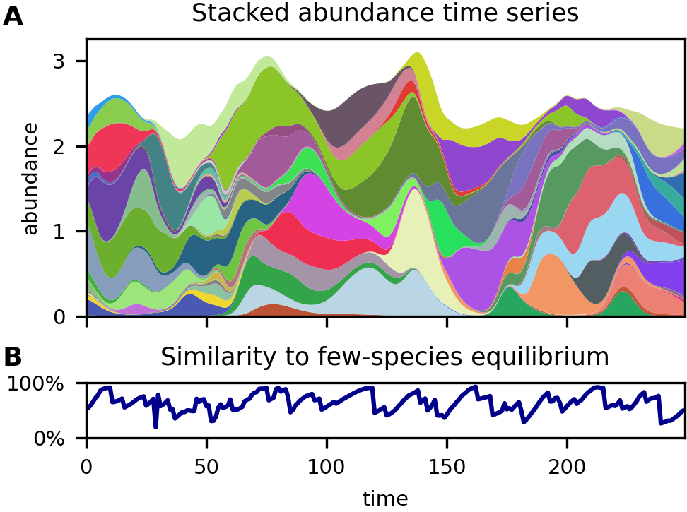
Figure 1: Turnover of the dominant component. A The stacked abundances of all species under steady-state conditions: there is a turnover of species such that only the dominant component is visible at any given time (each species has a distinct random colour). B Bray-Curtis index of community composition similarity between the dominant component of the community at time $t$, and the composition if it were isolated from the rare species and allowed to reach equilibrium: the community appears to approach the composition of few-species equilibria before being destabilized by invasion from the pool of rare species.

A chaotic turnover of rare and abundant species

For a broad range of parameters in strong-interaction regime, the community undergoes a chaotic turnover of dominant species. As illustrated by the time series of stacked abundances in Figure 1A, the overwhelming share of the total abundance at any given time is due to just a few species. Which species are abundant and which are rare changes on a characteristic timescale, $\tau_{\text{dom}}\approx 30$ time units, comparable to the time it would take an isolated species to attain an abundance on the order of its carrying capacity, starting from the lowest abundance set by immigration ($-\ln\lambda\approx 18$). While the total abundance fluctuates moderately around a well-defined time average, individual species follow a ‘boom-bust’ dynamics. If this simulation represented a natural community, only the most abundant species—that we call the dominant component of the community—would be detectable by morphological inspection or shallow sequencing.

We wish to characterize the dominant component, and understand how it relates to the pool of rarer species. In order to quantify the notion of dominance, we define the effective size of the community as Simpson’s (reciprocal) diversity index [51],

$$S_{\text{eff}}(t):=\frac{1}{\sum_{i}p_{i}^{2}(t)},$$ (6)

where $p_{i}=x_{i}/\sum_{j}x_{j}$ denote relative abundances. $S_{\text{eff}}$ approaches its lowest possible value of $1$ when a single species is responsible for most of the total abundance, and its maximum $S$ when all species have similar abundances. Its integer approximation provides the richness, i.e. number of distinct species, of the dominant component.

The effective size $S_{\text{eff}}$ of the community in our reference simulation fluctuates around an average of 9 dominant species, which make up $90\%$ of the total abundance. The relative abundance threshold for a species to be in the dominant component fluctuates around $3\%$, which is comparable to the arbitrary $1\%$-threshold used in empirical studies [9]. In Supplementary Figure LABEL:supp:fig:Seff we show that the number of dominant species grows slowly (but super-logarithmically) with $S$, up to about 15 for $S=10^{4}$. Thus, strong interactions limit the size of the dominant component and the vast majority of species are rare at any point in time.

The turnover of dominant species is not periodic; indeed, even over a large time-window, where every species is found on multiple occasions to be part of the dominant component, its composition never closely repeats (Supplementary Figure LABEL:supp:fig:tempsim). This aperiodicity suggest the presence of chaotic dynamics. We give numerical evidence for sensitive dependence on initial condition and positive maximal Lyapunov exponent in Supplementary Figure LABEL:supp:fig:sens and LABEL:supp:fig:lya. The turnover dynamics has the character of moving, chaotically, between different quasi-equilibria corresponding to different compositions of the dominant community (cf. ‘chaotic itinerancy’ [52]). To reveal this pattern, we measure a ‘closeness-to-equilibrium’, defined as the similarity in composition between the observed dominant component at a given time, and the equilibrium that this dominant component would converge to if it were isolated from the rare component and allowed to equilibrate. As a similarity metric we use the classical Bray-Curtis index (Appendix B), which has also been used to measure variations in community composition in plankton time series[17]. In Figure 1B, we see that the similarity at times slowly approaches $100\%$, followed by faster drops, towards about $50\%$, indicating the subversion of a coherent dominant community by a previously rare invader.

The fact that the community composition is not observed to closely repeat is arguably due to the vast number of possible quasi-equilibria that the chaotic dynamics can explore. In the weak-interaction regime, a number of unstable equilibria exponential in $S$ has been confirmed [53, 54]. It is therefore conceivable that the number of quasi-equilibria in our case is also exponentially large. The LV equations for $\lambda=0$ admit up to one coexistence fixed point (not necessarily stable) for every chosen subset of species [46]. Hence, we expect on the order of $\sim S^{S_{\text{eff}}}$ quasi-equilibria, which for $S_{\text{eff}}\approx 9$ evaluates to $10^{24}$! If the dynamics explores the astronomical diversity of such equilibria on trajectories which depend sensitively on the initial conditions, the dominant component may look as if having been assembled ‘by chance’ at different points in time.

The composition of the dominant community is not entirely arbitrary, though. While the abundance time series of most pairs of species have negligible correlations, every species tends to have a few other species with a moderate degree of correlation. In particular, if $(\alpha_{ij}+\alpha_{ij})/2$ is significantly smaller than the expectation $\mu$, and hence species $i$ and $j$ are close to a commensal or mutualistic relationship, these species tend to ‘boom’ one after the other (Supplementary Figure LABEL:supp:fig:corr).

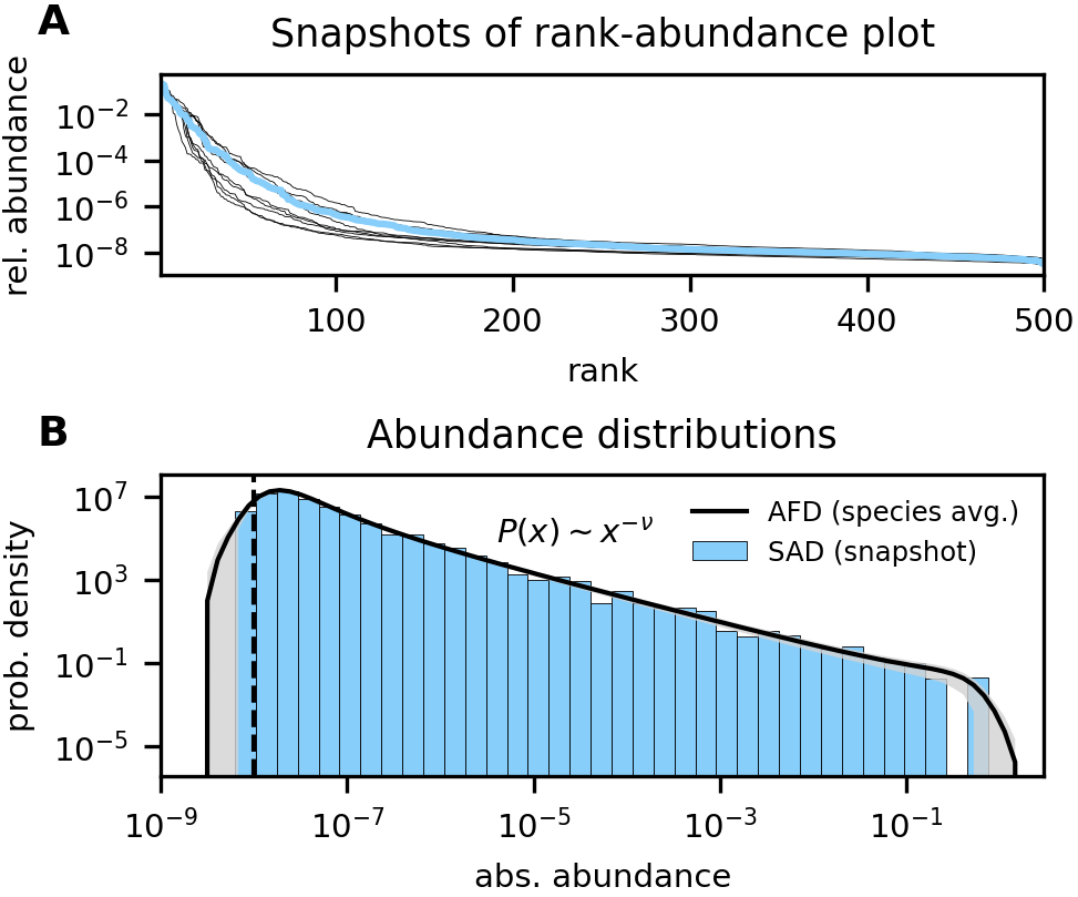
Figure 2: Statistical features of abundance variations across species and in time. A Snapshot rank-abundance plot for the relative abundances in the reference simulation: most species have orders of magnitude smaller abundances than the top ranks. Different lines represent observations at well-separated time points. B Species abundance distribution (SAD, blue histogram) corresponding to the blue rank-abundance plot; overlaid, abundance fluctuation distribution (AFD), averaged over all species (black line) with $\pm$ one standard deviation across species shaded in grey: the snapshot SAD appears to be a subsampling of the average AFD, indicating an equivalence, but de-synchronization, of species in their abundance fluctuations. The one bar missing from the SAD is the effect of finite species richness, as high-abundance bins only ever contain a couple of species for $S=500$. The vertical dashed line indicates the immigration level which determines a lower limit to abundances.

Species’ abundance fluctuations follow a power-law

In a common representation of empirical observations, where relative abundances are ranked in descending order (a rank–abundance plot [55]), microbial communities display an overwhelming majority of low-abundance species [5]. Our simulated community reproduces this feature; Figure 2A. The exact shape of the plot changes in time, as does the rank of any particular species, but the overall statistical structure of the community is highly conserved. An alternative way to display the same data is to bin abundances, and count the frequency of species occurring within each bin, producing a species abundance distribution (SAD) [55]. The histogram in Figure 2B illustrates the ‘snapshot’ SAD for the rank-abundance plot in Figure 2A of abundances sampled at a single time point. Whenever observations are available for multiple time points, it is also possible to plot, for a given species, the histogram of its abundance in time. As time gets large (practically, we considered $100`000$ time units after the transient), the histogram converges to a smooth distribution, that we call the abundance fluctuation distribution (AFD) [38]. Its average shape across all species is also displayed in Figure 2B.

Several conclusions can be drawn by comparing SADs and AFDs. First, a snapshot SAD appears to be a subsampling of the average AFD. Therefore, SADs maintain the same statistical structure despite the continuous displacement of single species from one bin to another. Second, every species fluctuates in time between extreme rarity ($x\approx\lambda=10^{-8}$) and high abundance ($x\gtrsim 10^{-1}$). This variation is comparable to that observed, at any given time, between the most abundant and the rarest species. Third, species are largely equivalent with respect to the spectrum of fluctuations in time, as indicated by the small variation in AFDs across species. We will evaluate the regularities and differences of single-species dynamics more thoroughly in Section 3.4.

The most striking feature of these distributions, however, is the power-law $x^{-\nu}$ traced for intermediate abundances. This range is bounded at low abundances by the immigration rate and at high abundances by the single-species carrying capacity. The power-law exponent is $\nu\approx 1.18$ for the simulation analysed, but it varies in general with the ecological parameters, as we discuss further in the following sections.

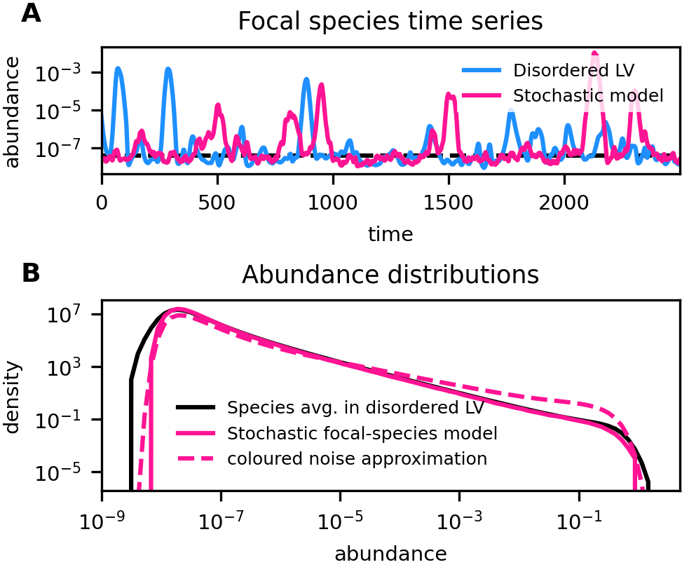
Figure 3: Comparison of the stochastic focal-species model and the chaotic dLV model. A Time series of one arbitrary species in the disordered Lotka-Volterra (dLV) model (blue), and one realization of the stochastic focal-species model (Eq. (7)) with parameters as in Eq. (9): the time series are statistically similar. B Comparison of the average abundance fluctuation distribution (AFD) from Figure 2 (black), and the AFD of the focal-species model (pink): excellent agreement is found for the power-law section. The ‘unified coloured noise approximation’ solution for the focal-species model’s AFD (dashed, pink line) predicts the correct overall shape of the distribution, but not a quantitatively accurate value for the power-law exponent.

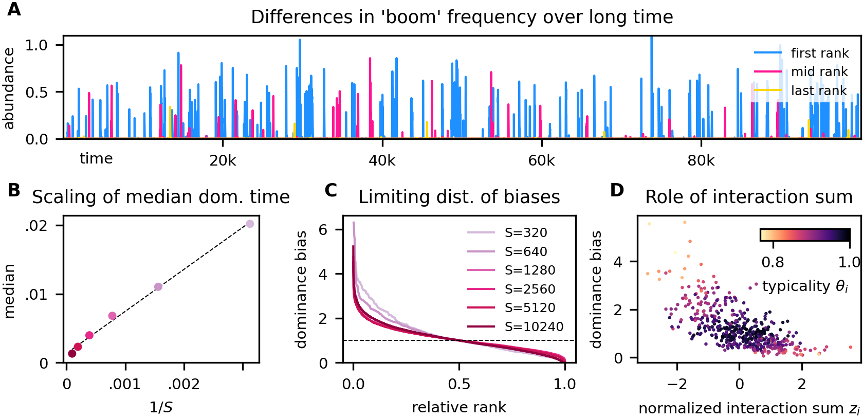
Figure 4: Species differences in dominance. A Example of a long abundance time series for the three species who are ranked first, median, and last, with respect to the ‘dominance bias’ (fraction of time spent in the dominant component relative to the species median). Some species ‘boom’ more often than others. B The scaling of median fraction of time spent in the dominant component against reciprocal species pool size: increasing $S$ results in a proportional decrease in median dominance time. C Distribution of dominance biases against relative dominance rank for a range of $S$: there appears to be convergence towards a non-constant limiting distribution, implying that net species differences are not due to small-$S$ effects. Note that, by definition, the dominance bias is $1$ for the middle rank, indicated by the dashed line separating positively from negatively biased species. D Scatter of dominance bias against the normalized sum of interaction coefficients, $z_{i}$ Eq. (4): lower net competition correlates with higher dominance bias. Species in the tails of the $z_{i}$ distribution are also less ‘typical’, with typicality quantified by the index $\theta_{i}$, Eq. (16), representing the similarity of a species AFD to the species-averaged AFD. Panel A and D are both for $S=500$.

The regularity of the abundance distributions across species suggests that it may be possible to describe the dynamics of a ‘typical’ species in a compact way—this is the goal of the next section.

A stochastic focal-species model reproduces boom-bust dynamics

Fluctuating abundance time series are often fitted by one-dimensional stochastic models [15]; for example, stochastic logistic growth has been found to capture the statistics of fluctuations in a variety of data sets on microbial abundances [38, 39]. The noise term encapsulates variations in a species’ growth rate whose origin may not be known explicitly. In our virtual Lotka-Volterra community, once the interaction matrix and initial abundances have been fixed, there is no uncertainty; nonetheless, the chaotic, high-dimensional dynamics results in species’ growth rates fluctuating in a seemingly random fashion. We are therefore led to formulate a model for a single, focal species, for which explicit interactions are replaced by stochastic noise. Because we have found species to be statistically similar, its parameters do not depend on any particular species, but reflect thee effective dynamics of any species in the community.

Following dynamical mean-field-like arguments and approximations informed by our simulations (Appendix E), we derive the focal-species model

$$\dot{x}(t) =x(t)\,(g(t)-x(t))+\lambda,$$ (7a)

$$g(t) =-k+u\,\eta(t),$$ (7b)

where $g(t)$ is a stochastic growth rate with mean $-k$, and fluctuations of magnitude $u$ and correlation time $\tau$. The process $\eta(t)$ is a coloured Gaussian noise with zero mean and an autocorrelation that decays exponentially;

$$\langle\eta\rangle=0,\quad\langle\eta(t)\,\eta(t^{\prime})\rangle=e^{-|t-t^{\prime}|/\tau},$$ (8)

where brackets denote averages over noise realizations. The connection between the ecological parameters $S,\mu,\sigma,\lambda$ and the resulting dynamics of the disordered Lotka-Volterra model in the chaotic phase is then broken down into two steps: how the effective parameters $k,u,\tau$ relate to the ecological parameters; and how the behaviour of the focal-species model depends on the effective parameters.

For the first step we find

$$k=\mu\overline{X}-1\quad\text{and}\quad u=\sigma\frac{\overline{X}}{\sqrt{\overline{S}_{\text{eff}}}},$$ (9)

where $X$ is the total community abundance of the original dynamics Eq. (1), the effective community size $S_{\text{eff}}$ is as in Eq. (6), and an overline denotes a long-time average. Equation (9) relates the focal species’ growth rate to the time-averaged net competition ($\approx\mu\overline{X}$) from all other species. We find in simulations of Eq. (1) in the chaotic phase that competition is strong enough to make $k>0$. The second relation captures the variation in the net competition that a species experiences because of turnover of the dominant community component. Due to sampling statistics, this variation is larger when the dominant component tends to have fewer species; hence the dependence on $(\overline{S}_{\text{eff}})^{-1/2}$. The third effective parameter, the timescale $\tau$, controls how long the focal species stays dominant, once a fluctuation has brought it to high abundance. This timescale is essentially equal to the turnover timescale $\tau_{\text{dom}}$ of the dominant component (defined more precisely by autocorrelation functions in Appendix E). In the weak-interaction regime, where any pair of species can be treated as effectively independent at all times, self-consistency relations such as $S\langle x\rangle=\overline{X}$ allow to implicitly express the focal-species model in terms of the ecological parameters. For strong interactions, however, the disproportionate effect of the few dominant species on the whole community invalidates this approach; we therefore relate the effective parameters to the community-level observables $\overline{X}$, $\overline{S}_{\text{eff}}$, $\tau_{\text{dom}}$ which are obtained from simulation of Eq. (1) at given values of the ecological parameters.

For the second step, we would like to solve Eqs. (7) for general values of the effective parameters. While this is intractable due to the finite correlation time of the noise, the equations can be simulated and treated by approximate analytical techniques. In Figure 3A we compare the time series of an arbitrary species in the dLV model with a simulation of the focal-species model. By eye, the time series appear statistically similar. The typical abundance of a species can be estimated by replacing the fluctuating growth rate in in Eq. (7) with its typical value (i.e. $\eta=0$), yielding the equilibrium $\lambda/k$ if $k>0$, as indeed confirmed by the simulation. Thus the typical abundance value is on the order of the immigration threshold. Figure 3B shows that the average AFD of the dLV agrees remarkably well with the stationary distribution of the focal-species model, in particular for the power-law section. Using the unified coloured noise approximation [56] (Appendix F), one predicts that the stationary distribution, for $\lambda\ll x\ll 1$, takes the power-law form $x^{-\nu}$, where the exponent

$$\nu=1+\frac{k}{u^{2}\tau}.$$ (10)

is strictly larger than one—the value predicted for weak interactions [30] and for neutral models [57]. Even if Eq. (10) is not quantitatively precise (Figure 3B), this formula suggests a scaling with the effective parameters that we will discuss later on.

Species with lower net competition are more often dominant

The similarity of all species’ abundance fluctuation distributions in Figure 2 is reflected in the focal-species model’s dependence on collective properties like the total abundance. However, the logarithmic scale downplays the variance between species’ AFDs, particularly at higher abundances. Indeed, while all abundances fluctuate over orders of magnitude, some species are observed to be more often dominant (or rare). Such differences are reminiscent of the distinction between ‘frequent’ and ‘occasional’ species observed in empirical time series [58, 59].

In order to assess the nature of species differences in simulations of chaotic dLV, we rank species by the fraction of time spent as part of the dominant component. Observing the community dynamics on a very long timescale (400 times longer than in Figure 1), the first-ranked species appears to boom much more often than the last (Figure 4A). The frequency of a species is chiefly determined by the number of booms rather than their duration, which is comparable for all species. The median dominance time decreases with the total species richness (Figure 4B): a doubling of $S$ leads to each species halving its dominance time fraction. As the community gets crowded—while its effective size hardly increases, as remarked in Section 3.1—all species become temporally more constrained in their capacity to boom. Yet some significant fraction of species is biased towards booming much more often or rarely than the median, regardless of community richness. We quantify this trend by plotting in Figure 4C the dominance bias—the dominance time fraction normalized by the median across all species—against the relative rank (i.e., rank divided by $S$). For high richness ($S\sim 10^{3}$), the distribution of bias converges towards a characteristic, nonlinearly decreasing shape, where the most frequent species occur more than four times as often as the median, and the last-ranked species almost zero.

The persistence of inter-species differences with large $S$ may seem to contradict the central limit theorem, as the vectors of the interaction coefficients converge towards statistics that are identical for every species. In the chaotic regime, however, even the smallest differences in growth rates get amplified during a boom. As we show in Appendix D, if Eq. (1) is rewritten in terms of the proportions $p_{i}$, the relative advantage of species $i$ is quantified by a selection coefficient whose time average scales as $-S^{-1/2}\sigma z_{i}$. Correspondingly, the relative, time-averaged growth rate is proportional to the net interaction bias $z_{i}$ (defined in Eq. (4)), resulting in species with larger $z_{i}$ to have positive dominance bias (Figure 4D). Outliers of the scatter plot, i.e. species that have particularly high or low dominance ranks, are also the species whose AFD is furthest from the average AFD of the community, as quantified by the typicality index $\theta_{i}\in[0,1]$, defined in Appendix B.

In conclusion, the relative species-to-species variation in the total interaction strength drives the long-term differences in the dynamics of single species in the community. While the focal-species model emphasizes the similarity of species, species differences can also be taken into account by employing species-specific effective parameters. In particular, replacing $k$ with a distribution of $k_{i}$’s would create a dominance bias, and is in fact motivated upon closer examination of our focal-species model derivation (Figure 7D in Appendix E).

Interaction statistics control different dynamical phases

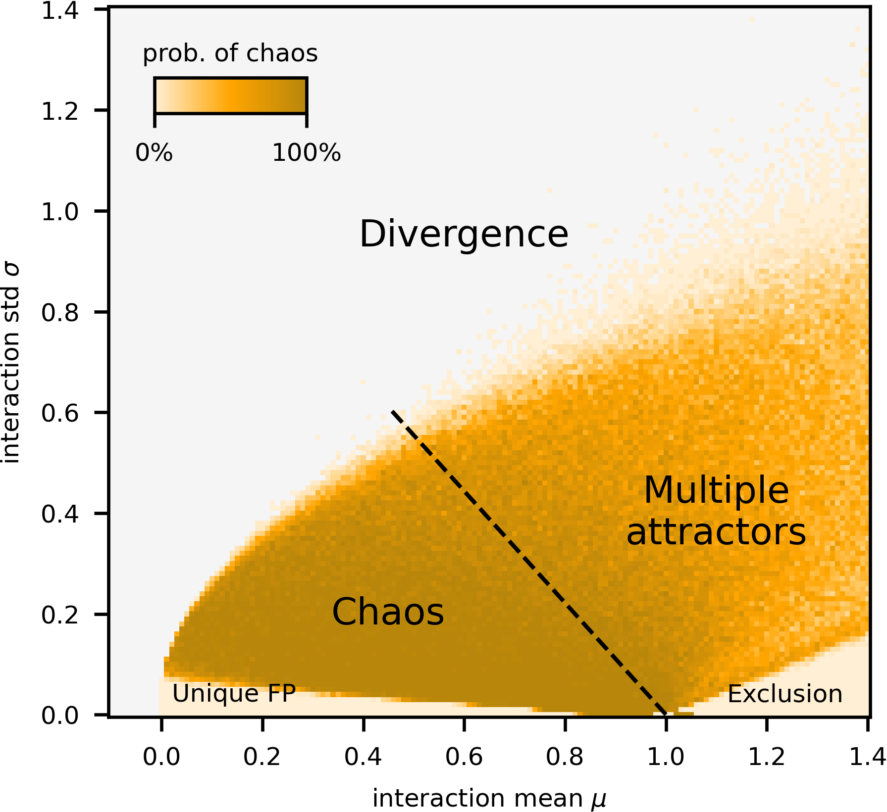
Figure 5: Dynamical phases of the disordered Lotka-Volterra model as a function of the interaction mean and standard deviation. Probability of persistent chaos in long-time simulations: for each $\mu$ and $\sigma$ (with 0.01 increment), $30$ simulations were made, each with a different random initial condition $x_{i}\sim U(\lambda,2/S)$ and realization of the interaction matrix. Parameters yielding divergence every time are marked with grey. The boundary separating the chaotic phase from the rest of the multiple-attractor phase (in which cycles and multi-stable fixed point are common in addition to chaos) is not sharp, unless probed adiabatically in the way explained in Supplementary Figure LABEL:supp:fig:adiab. The unique fixed-point phase has been studied analytically in the weak-interaction regime ($\mu\sim 1/S$). When inter-specific competition is in general stronger than intra-specific competition, a single species (identity depending on initial condition) dominates, in line with the classical competitive exclusion principle [60].

Hitherto, we have focussed on reference values of the interaction statistics $\mu$ and $\sigma$ that produce chaotic turnover of species abundances. We now broaden our investigation to determine the extent of validity of our previous analysis when the interaction statistics are varied. For every pair of $(\mu,\sigma)$ values, we run 30 independent simulations, each with a different sampling of the interaction matrix and uniformly sampled abundance initial condition. After a transient has elapsed, we classify the trajectory as belonging to one of four different classes: equilibrium, cycle, chaos, or divergence. Figure 5 displays the probability of observing chaos, demonstrating that it does not require fine tuning of parameters, but rather occurs across a broad parameter range.

The parameter region where chaos is prevalent, the ‘chaotic phase’, borders on regions of qualitatively different community dynamics. For small variation in interaction strengths (below the line connecting $(-1/S,\sqrt{2/S})$ to $(1,0)$), the community has a unique, global equilibrium that is fully characterized for weak interactions (cf. Fig. 2. of [25]). The transition from equilibrium to chaos has been investigated with dynamical mean-field theory [30]. For low interaction variance, but with mean exceeding the unitary strength of intra-specific competition, a single species comes to dominate, as expected by the competitive exclusion principle [60]. Adiabatic simulations, implemented by continuously rescaling a single realization of the interaction matrix (details in Supplementary Figure LABEL:supp:fig:adiab), reveal that lines radiating from the point $(\mu,\sigma)=(1,0)$ separate sectors where stable fixed points have different numbers of coexisting species. Traversing these sectors anti-clockwise, $S_{\text{eff}}$ increases by near-integer steps from one (full exclusion) up to about 8. From thence, a sudden transition to chaos occurs at the dashed line in Figure 5. We note, however, that the parameter region between chaos and competitive exclusion contains attractors of different types: cycles and chaos, coexisting with multiple fixed points, resulting in hysteresis (Supplementary Figure LABEL:supp:fig:adiabB). This ‘multiple attractor phase’ [25, 30] is a complicated and mostly uncharted territory whose detailed exploration goes beyond the scope of this study. Finally, for large variation in interactions, some abundances diverge due to the positive feedback loop induced by strongly mutualistic interactions, and the model is biologically unsound.

Across the phase diagram, community-level observables such as the average total abundance $\overline{X}$ and effective community size $\overline{S}_{\text{eff}}$ vary considerably (Supplementary Figure LABEL:supp:fig:commobs). The weak-interaction regime (whether in the equilibrium or chaotic phase) allows for high diversity, so $\overline{X}$ and $\overline{S}_{\text{eff}}$ are of order $S$; strong interactions, on the other hand, imply low diversity, with $\overline{S_{\text{eff}}}$ and $\overline{X}$ of order unity. An explicit expression for how these community-level observables depend on the ecological parameters ($S,\mu,\sigma,\lambda$) is intractable (although implicit formulas exists in the weak-interaction regime [25]). Nonetheless, an approximate formula that we derive in Appendix C allows to relate community-level observables to one another and to $\mu$ and $\sigma$:

$$\overline{X}\approx\left[\mu+\frac{1-\mu}{\overline{S}_{\text{eff}}}-\sigma\overline{\rho}\right]^{-1},$$ (11)

in which we introduce the collective correlation

$$\overline{\rho}:=-\sum_{ij}z_{ij}\overline{p_{i}p_{j}},$$ (12)

involving the time-averaged product of relative abundances weighted by the their normalized interaction coefficient Eq. (4). By construction, the collective correlation is close to zero when all species abundances are uncorrelated over long times, as would follow from weak interactions. On the contrary, it is positive when pairs of species with interactions less-competitive than average tend to co-occur, and/or those with more-competitive interactions tend to exclude one another.

Eq. (11) is particularly useful in understanding the role of correlations in the chaotic phase. As we observed in Section 3.3, the effective parameter $k=\mu\overline{X}-1$ is positive in the chaotic phase, implying that the growth rate of a species is typically negative, and abundances are therefore typically on the order of the small immigration rate rather than near carrying capacity. The existence of these two ‘poles’ of abundance values is key to boom-bust dynamics. By combining $k>0$ with Eq. (11), we estimate a minimum, critical value of the collective correlation required for boom-bust dynamics:

$$\rho_{\text{c}}=\frac{1-\mu}{\sigma}\frac{1}{\overline{S}_{\text{eff}}}.$$ (13)

Numerical simulations demonstrate that $\overline{\rho}\gtrsim\rho_{c}$ in the chaotic phase, where the critical value is approached at the boundary with the unique-equilibrium phase (Supplementary Figure LABEL:supp:fig:critcorr). With this result in hand, Eq. (11) and Eq. (13) establish that $\overline{X}\gtrsim 1/\mu$ in the chaotic phase. For strong interactions, total abundances are predicted to be of order one, and for weak interactions $\overline{X}\approx S/\tilde{\mu}$ (recall Eq. (5)), which recovers the observed scalings of these observables. As one moves deeper into the chaotic phase, the collective correlation increases continuously, as the effective community size drops, suggesting a seamless transition from a weak-interaction, chaotic regime amenable to exact treatment [30], to the strongly correlated regime that we have analyzed by simulations and the approximate focal-species model.

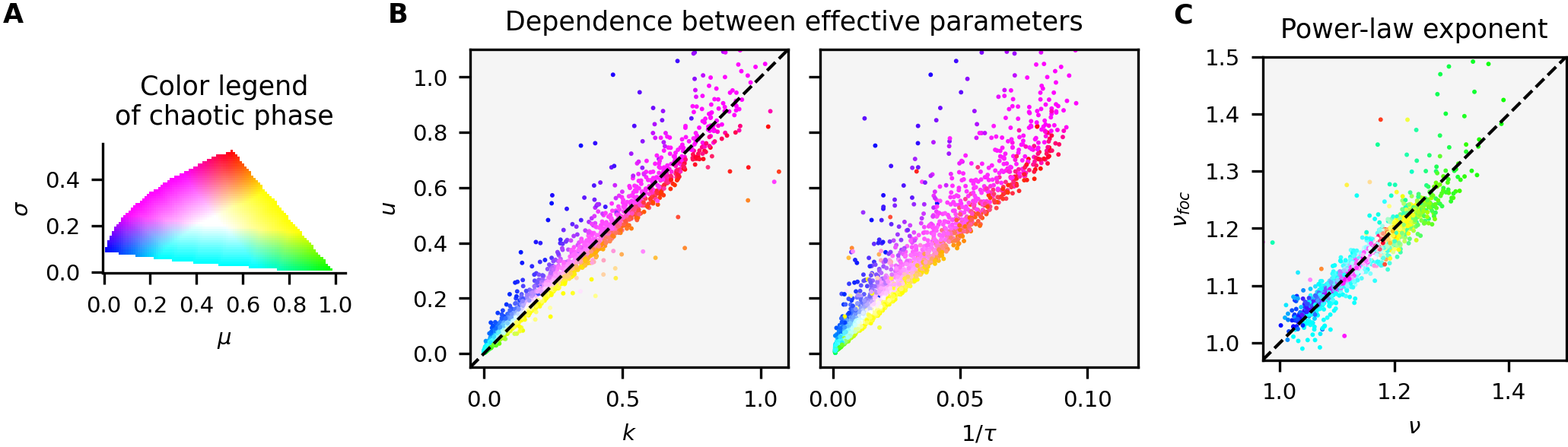
Figure 6: Relations between effective parameters in the chaotic phase. A Colour legend of the chaotic phase (boundaries from Figure 5). Each pair of $(\mu,\sigma)$ has been mapped to a distinct colour. B The exponent $\nu$ of the power-law section of the AFD for the chaotic dLV model plotted against the analogue $\nu_{\text{foc}}$ obtained for the focal-species model: generally good agreement is found, with more outliers for parameters close to phase boundaries. A few outliers lie beyond the plotted range. C Co-dependence of the effective parameters $u,k,\tau$: the amplitude $u$ of growth-rate fluctuations approximately equals the absolute value $k$ of the negative growth rate (only weakly depending on $\lambda$ and $S$; Supplementary Figure LABEL:supp:fig:kuscaling); $u$ is roughly proportional to the inverse turnover time, but the slope of the relationship depends on $\lambda$ and $S$.

Self-organization between community-level observables constrains abundance power-law variation

In Section 3.3 we established a focal-species model depending on the effective parameters $k,u,$ and $\tau$, that were related to the ecological parameters $S,\mu,\sigma,\lambda$ indirectly via community-level observables $\overline{X},\overline{S}_{\text{eff}},\tau_{\text{dom}}$. Furthermore, in the previous section we studied how the latter vary in the chaotic phase. Putting these results together, we here examine the corresponding variation of the effective parameters and of the focal-species model’s predictions.

Because the trio $k,u,\tau$ ultimately hails from but two independent variables, $\mu,\sigma$ (considering fixed $S$, $\lambda$), they must be dependent. Figure 6A demonstrates that, across the chaotic phase, an approximate linear relationship holds between $k$ and $u$, as well as between $u$ and $\tau$. Because $k$ and $u$ are related to the mean and the variance of abundances via Eq. (9), their proportionality is reminiscent of the empirical Taylor’s law which posits a power-law relation between abundance mean and variance as they vary across samples [61]. The slope of the relationship of $u$ to $k$ is close to one (and varying little with $S$ and $\lambda$; Supplementary Figure LABEL:supp:fig:kuscaling), which implies with Eq. (9) that

$$\overline{X}\approx\left[{\mu-\frac{\sigma}{\sqrt{\overline{S}_{\text{e}}}}}\right]^{-1}.$$ (14)

Comparison to Eq. (11) then yields that $\rho-\rho_{c}\approx\overline{S}_{\text{eff}}{}^{-1/2}$. This empirical relationship thus supports the aforementioned convergence—in the limit where $\overline{S}_{\text{eff}}$ is large, as for weak interactions—of the collective correlation to its critical value.

We find in Figure 6 that the slope $\nu_{\text{foc}}$ of the power-law trend obtained from simulation of the focal-species model finds good agreement with the value $\nu$ from the full dLV model. There is a narrow overall variation of the exponent; a consequence of the interdependency of the effective parameters. As can be intuited by the approximate expression Eq. (10) for the focal-species model, the exponent is strictly larger than $1$, a value it approaches if the turnover time scale diverges, as indeed it does on the boundary to the unique equilibrium phase. The exponent increases as interactions become more competitive, up to about $1.4$ at $(\mu,\sigma)=(1,0)$. However, the exponent also depends on $S$ and $\lambda$, showing a constant slope against $\log S$ or $-1/\log\lambda$ (Supplementary Figure LABEL:supp:fig:nuscaling).

Discussion

We have sought a possible theoretical underpinning for macroecological patterns of dominance and rarity in species-rich communities. To this end, we studied a Lotka-Volterra model with strong interactions and weak immigration using numerical simulations and approximate analytical techniques. We characterized a parameter regime where species generically turn over between a small dominant component, and a large pool of temporarily rare species. In this process, each species’ abundance undergoes a chaotic boom-bust dynamics, asynchronous with respect to most other species. The resulting distribution of abundances—of a single species over long times, or of the whole community at a single time—has a prominent power-law trend.

The phenomenology of the model—chaos, boom-bust dynamics, and a power-law shaped SAD with exponent larger than one—is consistent with observations of marine plankton communities [3, 12, 62, 18, 16]. While the evidence for chaos in ecological time series has been generally ambiguous, a recent systematic assessment concludes that chaos is commonplace, especially for plankton [16]. Experiments with closed plankton microcosms have revealed chaotic, high-amplitude fluctuations sustained over many years [12, 62]. Abundance fluctuations indicative of chaos were also seen in non-planktonic synthetic microbial communities [63, 13], but of lower amplitude. That planktonic population sizes fluctuate over many orders of magnitude in abundance is made especially poignant by algal blooms, which can become visible even from space. The timing of blooms, and the succession of functional groups within a season, are coupled to environmental factors such as nutrient concentrations. Yet, for the non-dominant taxa, the large differences in a species’ abundance between ocean samples show little environmental signature [3]. This suggests that the turnover of abundances might rather be driven by complex interactions or mixing dynamics. Empirical snapshot SADs of marine protists show a clear power-law trend for non-dominant species within the same size class, with a larger-than-one exponent varying little between samples, as in our model.

The empirical value of the exponent $\nu$ of the SAD’s power-law trend (around 1.6 [3]) is important because it rules out particular model assumptions. The chaotic phase in the Lotka-Volterra model produces a unitary exponent in the weak-interaction limit, and seemingly also for strong interactions if the immigration rate vanishes, $\lambda\to 0$. Similarly, neutral theory predicts a power-law tail of the SAD with exponent one [64, 57]. To approach the empirical value, previous studies augmented neutral theory with nonlinear growth rates or chaotic mixing [3, 65] to find an exponent dependent on the model parameters. For dLV with strong interactions, we have shown that $\nu>1$ for all parameter combinations within the chaotic phase when interactions are strong. The approximate solution to the focal-species model, Eq. (10), shows that the positive deviation from $\nu=1$ depends on three inter-related effective parameters: the mean, amplitude, and timescale of fluctuations in each species’ net competition. As these fluctuations drive the turnover pattern, boom-bust dynamics comes to be associated to a larger-than-one exponent. In our model, $\nu$ approaches the empirical value in the green region of Figure 6A. There, interactions are strong (smaller than but relatively close to self-interactions) and vary moderately from species to species, and the turnover time scale is large (but not yet divergent). We can speculate that similar features underpin plankton ecological dynamics, and may differentiate these communities from other, more stable microbial assemblages.

The chaotic phase ends at the parameter point $(\mu,\sigma)=(1,0)$ where all non-divergent dynamical phases meet (Figure 5). These phases appear to be qualitatively similar to those observed in an individual-based version of the dLV model, accounting for demographic stochasticity [66]. There, the phases meet at the “Hubble point” which recovers neutral theory; every pair of individuals compete equally, and species only come to differ through randomness in birth-death events. Despite being deterministic, our model shows some similarity to neutral theory (sometimes referred to as effective neutrality [67, 68, 43]): species are largely equivalent in a statistical sense, and they fluctuate (pseudo-)randomly and mostly independently. It is important, however, to highlight the differences that allow distinguish between models. As argued before [33], the vast census sizes of planktonic species would imply enormous timescales of turnover if by demographic noise alone, the main driver of diversity in neutral models. In contrast, deterministic species interactions can produce rapid turnover. If the turnover time is long, or if there is no turnover, then species-specific AFDs would differ substantially from one another, and not span the range of abundances observed across the whole community. It is therefore informative to measure AFDs in addition the more commonly measured SADs, whenever this is feasible.

Fluctuations, whether due to demographic or environmental noise, or complex interactions, can drive species extinctions. In our model, the immigration term $\lambda$ represents some mechanism able to sustain abundances above the extinction threshold long enough for a species to rebound. Meta-community models of spatial patches connected by migration flows show how drastic levels of global extinctions can be avoided through a temporal storage effect [34, 33, 36, 35]: if the patches’ dynamics desynchronize, then a species that went extinct in one patch may eventually be re-established there through immigration from another patch where it persisted. Within-patch turnover of composition was observed in the meta-community setting but attributed to the local interactions in a single patch [33, 36]. In particular, Ref. [33] focussed on disordered Lotka-Volterra dynamics where both within- and between-species interactions follow the same statistics. This required anti-symmetric, i.e. predator-prey-paired, interactions ($\gamma=-1$) for sustained fluctuations. We have instead followed a competitive paradigm (normalized self-interaction, and $\gamma=0$), directly extending the studied range of the $\mu$–$\sigma$ phase diagram of earlier work [25, 30].

Furthermore, our model assumptions have allowed the formulation of an explicit focal-species model, in terms of a stochastic logistic equation with coloured noise. It is similar to models that have been successfully fitted to microbial time series [39, 38], but a notable difference lies in the negative mean growth rate we find, which together with noise-correlation and immigration yields fluctuations over many orders of magnitude. Our focal-species model constitutes an ecologically motivated candidate for fitting to ecological time-series with large fluctuations. Its derivation also serves an important conceptual purpose, as it illustrates in an ecological context how complex dynamics can come to resemble a simple noise process. Indeed, it is notoriously difficult to distinguish random noise from chaos in empirical time series. The prevalence of ecological chaos may have been underestimated for this reason [15, 16].

Chaos is a multifaceted phenomenon, and the question of how and why it arises in a given context is of great theoretical interest. It has long been recognized that Lotka-Volterra systems can admit heteroclinic networks [69, 70, 71]; saddle-points, i.e. equilibria with stable and unstable directions, connected by orbits. For LV equations without immigration, such saddles are found on the system boundary, corresponding to some subset of species having zero abundance (i.e. being extinct). One route to chaos is via the ‘deformation’ of a heteroclinic network, when, for instance, the introduction of an immigration term pushes saddles off the boundary. This can result in ‘chaotic intinerancy’, whereby trajectories traverse the vicinities of low-dimensional quasi-attractors (formerly saddles on the boundary) via higher-dimensional, chaotic phase-space regions [52, 72]. This picture fits well with our description of the chaotic turnover in relation to Figure 1. A further understanding of this mechanism may come from analytical investigations of disordered models related to, but more tractable than, Lotka-Volterra [73]; or focussing on the transition to chaos from the unique equilibrium regime in the weak-interaction limit of the dLV model. In the strong-interaction regime, a systematic bifurcation analysis of the transition from stable fixed points to chaos under the adiabatic scheme outlines in Supplementary Figure LABEL:supp:fig:adiab may also provide insights.

Our model can be extended in several directions. Differences in growth rates and carrying capacities between species are expected for natural communities, and revealed when fitting time series [74]; one may also consider a less than fully connected interaction network, e.g. sparsity [75, 76, 77]. Such generalizations will however break assumptions—in particular that of independent Gaussian interactions—underlying some of our analytical approximations. Preliminary numerical explorations suggest that existence of chaotic turnover dynamics is robust to these features, but that they may bias some species towards abundance or rarity (Supplementary Figure LABEL:supp:fig:robustness). A systematic investigation is however warranted. Given the proposed connection of our work to plankton ecology, considering a trophically structured ecosystem might be a particularly relevant generalization, as grazers [78] and viruses [79] have been put forward as key ecological actors. On the one hand, we have shown that non-structured competition between many species can produce high-dimensional chaos; on the other hand, the dynamics between functional groups such as bacteria, phyto- and zooplankton, and detrivores could potentially also be chaotic, but in low dimension. It is therefore an interesting question how fluctuations across different levels of coarse-graining of a community might be intertwined.

To conclude, we have demonstrated the emergence of a chaotic turnover of rare and abundant species in a strongly interacting community with minimal model assumptions. By deriving an explicit focal-species model to capture this complex dynamics, we have identified community-level observables and effective parameters that constrain the variation of the power-law exponent of the species abundance distribution. These insights may prove valuable for interpreting field data [3, 18], as well as for predicting dynamical features of synthetic communities [13].

Appendices

Numerical implementation

For Lotka-Volterra simulations we used a fixed time-step Euler scheme with $\Delta t=0.01$, applied to the logarithm of abundances. This guarantees the positivity of all abundances at all times, regardless of immigration rate. To automatically classify the long-time behaviour of trajectories as fixed-points, cycles, or chaos, we used a heuristic method of counting abundance vector recurrences, validated against visual inspection of trajectories and calculated maximal Lyapunov exponent for a subset of trajectories. Further details are given in Supplementary Note LABEL:supp:sec:scheme.

Similarity metrics

The Bray-Curtis similarity index [80] is defined as

$$\text{BC}(\boldsymbol{x},\boldsymbol{y})=\sum_{i}w_{i}\frac{\min(x_{i},y_{i})}{\text{mean}(x_{i},y_{i})},$$ (15)

where $w_{i}$ is the relative abundance of species $i$ with respect to the joined abundances $\boldsymbol{x}+\boldsymbol{y}$. By definition, $\text{BC}(\boldsymbol{x},\boldsymbol{y})=1$ iff $\boldsymbol{x}=\boldsymbol{y}$, and $\text{BC}\approx 0$ when, for each $i$, either $x_{i}\gg y_{i}$ or $y_{i}\gg x_{i}$; this makes it suitable for communities where abundances span orders of magnitude.

For the similarity graph Figure 1B, we have plotted $\text{BC}(\boldsymbol{x}^{\text{dom}}(t),\boldsymbol{y}^{*}(t))$, where $\boldsymbol{x}^{\text{dom}}(t)$ is the restriction of $\boldsymbol{x}(t)$ in the reference simulation to only the dominant species at time $t$, and $\boldsymbol{y}^{*}(t)$ is the fixed point reached from $\boldsymbol{x}^{\text{dom}}(t)$ as initial condition, with $\lambda=0$.

To compare the similarity the AFD of species $i$, $P_{i}(x)$, to the species-averaged AFD $P=\sum_{i}P_{i}/S$, we define the index

$$\theta_{i}:=1-\sup_{x}|F(x)-F_{i}(x)|,$$ (16)

where $F_{i}$ and $F$ are the cumulative distribution functions of $P_{i}$ and $P$, respectively; i.e., the index $\theta_{i}$ is based on the Kolmogorov-Smirnov distance [51] of the AFDs.

Derivation of time-averaged total abundance

Direct summation of Eq. (1) over $i$ (assuming $r_{i}=1$), and then division on both sides by $X(t)=\sum_{i}x_{i}(t)$, yields

$$\frac{\mathop{}\!\mathrm{d}}{\mathop{}\!\mathrm{d}t}\ln X(t)=1-X(t)\left[\mu+(1-\mu)/S_{\text{eff}}-\sigma\rho(t)\right]+\frac{S\lambda}{X(t)}$$ (17)

with $S_{\text{eff}}$ as in Eq. (6) and $\rho(t)$ as Eq. (12) but without the time average. We denote the time-average operator by

$$\mathbb{T}_{t}[f(t)]=\lim_{T\to\infty}T^{-1}\int_{0}^{T}\mathop{}\!\mathrm{d}t\,f(t).$$ (18)

Applying it to Eq. (17), the left-hand side becomes $\lim_{T\to\infty}(X(T)-X(0))/T$, which evaluates to zero on the assumption that no species diverges in abundance. The right-hand side contains terms such as $\mathbb{T}[X/S_{\text{eff}}]$ and $\mathbb{T}[X\rho]$. If the relative fluctuations in $X,S_{\text{eff}},\rho$ are small (see Supplementary Figure LABEL:supp:fig:commobs), or these functions are at most weakly correlated to one another, then we obtain, approximately,

$$0=1-\mu\overline{X}-(1-\mu)\overline{X}/\overline{S}_{\text{eff}}+\sigma\overline{\rho}+O(S\lambda).$$ (19)

As the immigration is small compared to the other terms it can be neglected; solving for $\overline{X}$ finds Eq. (11). The relative error in $\overline{X}$ between Eq. (11) for simulated values of the community-level observables in the right-hand side, and the simulated value of $\overline{X}$, is typically less than a few percent (see Supplementary Figure LABEL:supp:fig:Xerr).

Selective advantage

The dynamics of the relative abundance $p_{i}=x_{i}/X$, with $X=\sum_{j}x_{j}$, is found by summing and differentiating Eq. (1) as

$$\dot{p}_{i}=Xp_{i}\left\{\sum_{j}p_{j}^{2}-p_{i}-\sum_{j}p_{j}\left(\alpha_{ij}-\sum_{k}\alpha_{jk}p_{k}\right)\right\}\\ +\frac{\lambda S}{X}\left(\frac{1}{S}-p_{i}\right).$$ (20)

Using Eqs. (3), (6), and (12) in defining

$$\pi(t):=1/S_{\text{eff}}(t)-\sigma\rho(t),\quad s_{i}(t):=-\sigma\sum_{j}z_{ij}p_{j},$$ (21)

we can write Eq. (20) as

$$\dot{p}_{i}=Xp_{i}\left\{\pi+s_{i}-p_{i}\right\}+O(\lambda).$$ (22)

The term $s_{i}$ is responsible for the bias of species $i$ against the reference proportion $\pi$. As a heuristic means of calculating the time-averaged bias, we suppose the $p_{i}$’s can be treated independently of the $z_{ij}$ and be replaces by $\overline{p_{i}}\approx 1/S$; then we obtain $\overline{s}_{i}\approx-\sigma z_{i}/\sqrt{S}$. On this basis, we expect $z_{i}$ to be indicative of a species’ dominance bias.

Derivation of the stochastic focal-species model from dynamical mean-field arguments

We write Eq. (1) as

$$\dot{x}_{i}=x_{i}(g_{i}-x_{i})+\lambda,\quad g_{i}=1-\sum_{j(\neq i)}\alpha_{ij}x_{j}.$$ (23)

If we suppose that the abundances $\{x_{j}(t)\}$ (or, rather, their statistical properties) are independent of the particular realization $[\alpha_{ij}]$ of the interaction matrix, then, for a given realization of $\{x_{j}(t)\}$,

$$g_{i}(t)\sim\mathcal{N}\left(1-\mu\sum_{j(\neq i)}x_{j}(t),\ \sigma^{2}\sum_{j(\neq i)}x_{j}^{2}(t)\right),$$ (24)

based on the properties of sums of Gaussian variables. The time-varying mean and variance of $g_{i}$ means that, averaged over time, $g_{i}$ does not necessarily follow a Gaussian distribution. We introduce

$$a(t):=1-\mu\sum_{i}x_{i}(t),\quad b(t):=\sigma\sqrt{\sum_{i}x_{i}^{2}(t)},$$ (25)

which are found to exhibit significant relative fluctuations, with skewed distributions (Figure 7A and B). However, once we shift and scale $g_{i}(t)$ into the “effective noise”

$$\eta_{i}(t):=\frac{g_{i}(t)-a(t)}{b(t)},$$ (26)

we recover (closely) a $\mathcal{N}(0,1)$ distribution, for both the set $\{\eta_{i}(t)\}_{1,\ldots,S}$ at any given time $t$, or for the stationary distribution of $\eta_{i}(t)$, at least for typical species (Figure 7C and D). The empirical distribution of the $g_{i}$ across all species and times is closely approximated by the stationary distribution $\mathcal{N}(\overline{a},\overline{b})$ (Figure 7E). Therefore, we suppose that, despite their fluctuations, we can replace $a(t)$ and $b(t)$ with their time-averages and model $g_{i}$ as a stochastic process

$$g(t)=\overline{a}+\overline{b}\eta(t),$$ (27)

where $\eta(t)$ is a process with stationary distribution $\mathcal{N}(0,1)$. The parameter correspondence in Eq. (9) follows by $k=-\overline{a}$, $u=\overline{b}\approx\overline{X}/\sqrt{\overline{S}_{\text{eff}}}$, and $\tau=\tau_{\eta}$, the correlation time of $\eta$.

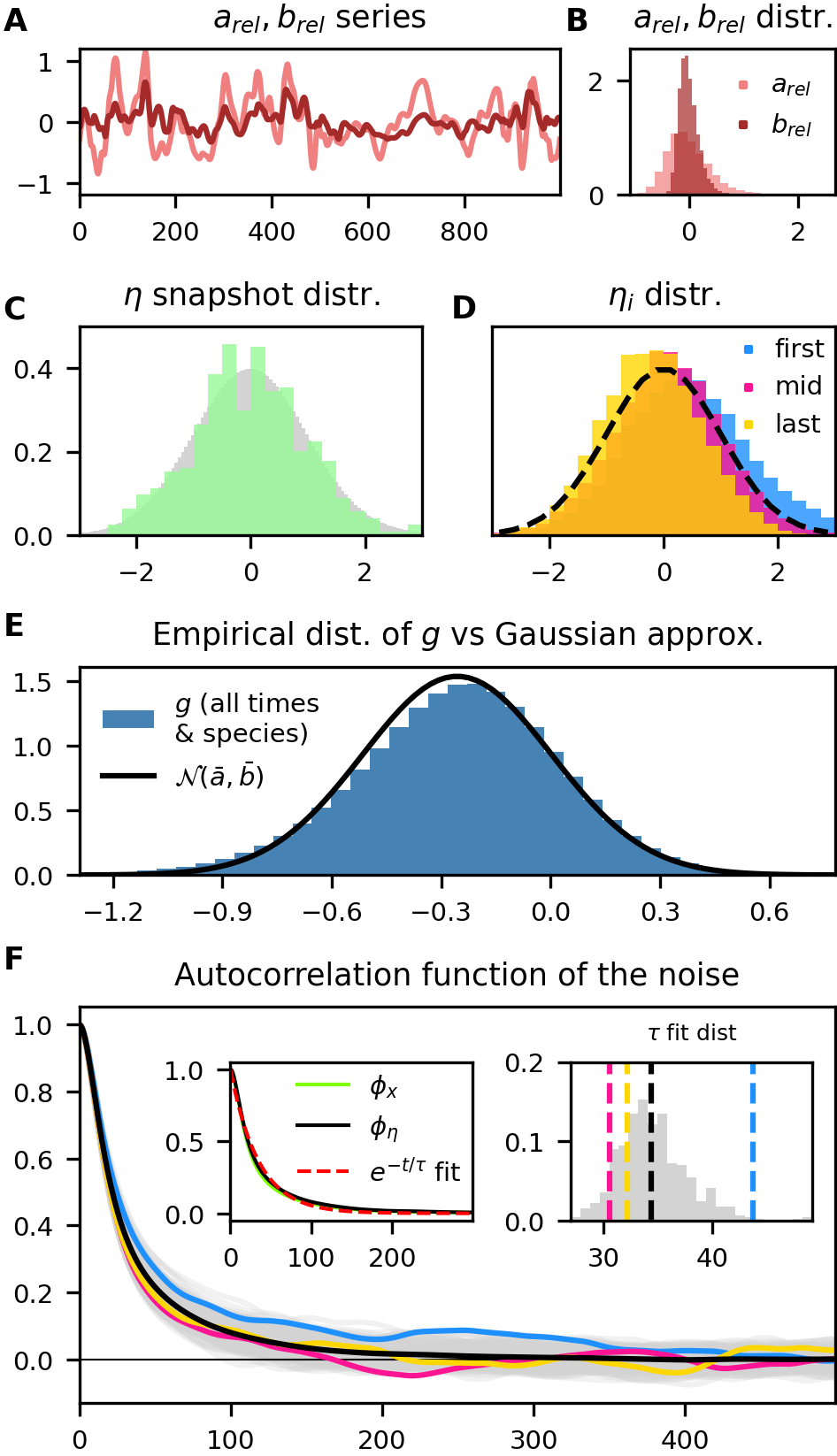
Figure 7: Statistical properties of the effective noise. A, B Time series and distribution of $a_{\text{rel}}=a/\overline{a}-1$, etc. C, D Histograms of $\eta_{i}(t)$ across all species and time (grey), over just species for one random time (green), over all time for the first/mid/last-ranked species with respect to average abundance (blue/pink/yellow), with $\mathcal{N}(0,1)$ (black, dashed) for reference. E The empirical distribution of $g$ in Eq. (23) over all species and times, compared to the distribution $\mathcal{N}(\overline{a},\overline{b})$ assumed for $g$ in the focal-species model. F Autocorrelation functions: for every species (grey), first/mid/last-rank species (blue/pink/yellow)), and the average over all species (black). The left inset compares the ACFs of $\boldsymbol{x}$ (green), $\eta$ (black), and the exponential fit to the latter (red); the right inset shows the distribution of the $\tau$ parameter in exponential fits to each species ACF.

Note that, up to neglecting a diagonal term of the sum, the effective noise can be written

$$\eta_{i}(t)=-\sum_{j(\neq i)}z_{ij}q_{j}(t),$$ (28)

with $z_{ij}\sim\mathcal{N}(0,1)$, and $\boldsymbol{q}(t)=\boldsymbol{x}(t)/||\boldsymbol{x}(t)||_{2}$. Given the chaotic turnover pattern, the latter is expected to perform something like a random walk on the $S$-sphere, with a de-correlation time corresponding to the turnover of dominant species. This timescale is inherited by the effective noise. More precisely, we compare autocorrelation functions (ACF). The ACF of a function $f$ is defined as

$$\phi_{f}(t_{\text{lag}}):=\frac{\mathbb{T}_{t}[\delta f(t)\cdot\delta f(t+t_{\text{lag}})]}{\text{Var}{f}},$$ (29)

with $\delta f=f-\overline{f}$ and using the notation Eq. (18). By definition $\phi_{f}(0)=1$. For each species’ effective noise we compute numerically $\phi_{\eta_{i}}(t_{\text{lag}})$, as shown in Figure 7F. Due to the small number of ‘booms’ per species, even over a large simulation time, ACFs are slightly irregular. In order to make estimations more accurate, we consider the averaged ACF

$$\phi_{\eta}:=\frac{1}{S}\sum_{i}\phi_{\eta_{i}}.$$ (30)

The decay of correlation is well-approximated by the exponential $\exp(-t_{\text{lag}}/\tau_{\eta})$, where the parameter $\tau_{\eta}$ (fitted by least squares) represents the noise correlation timescale for a ‘typical’ species.

The approximately $\mathcal{N}(0,1)$ distribution and exponential autocorrelation function of the effective noise $\eta$ suggest that it can be modelled as an Ornstein-Uhlenbeck process, the only Markov process with these two properties;

$$\dot{\eta}(t)=-\frac{1}{\tau}\eta(t)+\sqrt{\frac{2}{\tau}}\xi(t),$$ (31)

where $\xi(t)$ is a Gaussian white noise; $\langle\xi\rangle=0$, $\langle\xi(t)\xi(t^{\prime})\rangle=\delta(t-t^{\prime})$. The timescale referred to as $\tau_{\text{dom}}$ in the main text can be defined as $\tau_{\boldsymbol{x}}$, the decay time of the exponential fit to the ACF of the abundance vector. For a vector-valued function, Eq. (29) gives

$$\phi_{\boldsymbol{x}}=\frac{1}{S}\sum_{i}w_{i}\phi_{x_{i}},\quad w_{i}=\frac{\text{Var}[x_{i}]}{\frac{1}{S}\sum_{j}\text{Var}[x_{j}]}.$$ (32)

Comparing $\phi_{\eta}$ and $\phi_{\boldsymbol{x}}$, they match very well (inset of Figure 7F) for the reference simulation; as do the associated timescales $\tau_{\boldsymbol{x}}$ and $\tau_{\eta}$ for all $(\mu,\sigma)$ in the chaotic phase (Supplementary Figure LABEL:supp:fig:taux). This observation motivates identifying $\tau_{\eta}$ of the focal-species model with the turnover timescale $\tau_{\text{dom}}$. Thus, the focal species model and its parameters have been fully specified.

The crucial difference to dynamical mean-field theory developed in the weak-interaction limit is the fact that $a(t)$ and $b(t)$ are, for strong interactions, determined by a small number $(S_{\text{eff}})$ of dominant species, whose abundances fluctuate substantially, and, during their time of co-dominance, have significant effects on each other; i.e., they are conditionally correlated. Therefore, self-consistent determination of the effective parameters fails, because species cannot be treated as independent realizations of the focal-species model. For example, the self-consistency relation for $k$ in Eq. (7b) is $k=\mu S\langle x\rangle-1$. In our reference simulation $k=0.26$, whereas $\mu S\langle x\rangle-1=-0.31$ even has the wrong sign. This discrepancy is due to the neglected inter-species correlations needed for the collective correlation $\overline{\rho}$, Eq. (12), to exceed the critical value Eq. (13) associated with $k>0$ and boom-bust dynamics.

Steady-state solution of the focal-species model under the unified coloured noise approximation

The unified coloured noise approximation [56] assumes overdamped dynamics to replace a process $\dot{x}=F(x)+G(x)\eta$, driven by Gaussian correlated noise $\eta$ of correlation-time $\tau$, with a process driven by white noise. The approximation is exact in the limits $\tau\to 0$ or $\tau\to\infty$. The stationary distribution of the corresponding white-noise process is

$$P^{*}(x)\propto\exp\left\{\int^{x}v(x^{\prime})\mathop{}\!\mathrm{d}{x^{\prime}}\right\},$$ (33)

with

$$v=(\tau^{-1/2}H_{\tau})\frac{F}{G^{2}}+\left(\ln\frac{H_{\tau}}{G}\right)^{\prime},$$ (34)

and $H_{\tau}$ a function of $F$,$G$, and $\tau$. For Eq. (7)

$$F(x) =-x(k+x)+\lambda,$$ (35)

$$G(x) =ux,$$ (36)

$$H_{\tau}(x) =\tau^{-1/2}-\tau^{1/2}(x+\lambda x^{-1}).$$ (37)

With these functions, the integral in Eq. (33) can be performed exactly, yielding

$$P^{*}(x)=\frac{1}{\mathscr{N}}e^{-[q_{+}(x)+q_{-}(\lambda/x)]}x^{-\nu}\left(\tau^{-1}+x+\frac{\lambda}{x}\right),$$ (38)

expressed using the quadratic functions

$$q_{\pm}(y)=\frac{\left(y+(\tau^{-1}\pm k)\right)^{2}}{2u^{2}},$$ (39)

and $\nu$ given by Eq. (10).

References

- [1] Thompson LR, et al. (2017) A communal catalogue reveals Earth’s multiscale microbial diversity. Nature 551(7681):457–463.
- [2] Sogin ML, et al. (2006) Microbial diversity in the deep sea and the underexplored “rare biosphere”. Proceedings of the National Academy of Sciences 103(32):12115–12120.
- [3] Ser-Giacomi E, et al. (2018) Ubiquitous abundance distribution of non-dominant plankton across the global ocean. Nature Ecology & Evolution 2(8):1243–1249.
- [4] Eguíluz VM, et al. (2019) Scaling of species distribution explains the vast potential marine prokaryote diversity. Scientific Reports 9(1).
- [5] Lynch MDJ, Neufeld JD (2015) Ecology and exploration of the rare biosphere. Nature Reviews Microbiology 13(4):217–229.
- [6] Hoffmann KH, et al. (2007) Power law rank-abundance models for marine phage communities. FEMS Microbiology Letters 273(2):224–228.
- [7] Driscoll WW, Hackett JD, Ferrière R (2016) Eco-evolutionary feedbacks between private and public goods: evidence from toxic algal blooms. Ecology Letters 19(1):81–97.
- [8] Nemergut DR, et al. (2011) Global patterns in the biogeography of bacterial taxa. Environmental Microbiology 13(1):135–144.
- [9] Logares R, et al. (2014) Patterns of Rare and Abundant Marine Microbial Eukaryotes. Current Biology 24(8):813–821.
- [10] Chesson P (2000) Mechanisms of Maintenance of Species Diversity. Annual Review of Ecology and Systematics 31(1):343–366.
- [11] Lennon JT, Jones SE (2011) Microbial seed banks: the ecological and evolutionary implications of dormancy. Nature Reviews Microbiology 9(2):119–130.
- [12] Benincà E, et al. (2008) Chaos in a long-term experiment with a plankton community. Nature 451(7180):822–825.
- [13] Hu J, Amor DR, Barbier M, Bunin G, Gore J (2022) Emergent phases of ecological diversity and dynamics mapped in microcosms. Science 378(6615):85–89.
- [14] Huisman J, Weissing FJ (1999) Biodiversity of plankton by species oscillations and chaos. Nature 402:407–410.
- [15] Rogers TL, Johnson BJ, Munch SB (2022) Chaos is not rare in natural ecosystems. Nature Ecology & Evolution 6:1105–1111.
- [16] Munch SB, Rogers TL, Johnson BJ, Bhat U, Tsai CH (2022) Rethinking the prevalence and pelevance of chaos in ecology. Annual Review of Ecology, Evolution, and Systematics 53(1):227–249.
- [17] Fuhrman JA, Cram JA, Needham DM (2015) Marine microbial community dynamics and their ecological interpretation. Nature Reviews Microbiology 13(3):133–146.
- [18] Martin-Platero AM, et al. (2018) High resolution time series reveals cohesive but short-lived communities in coastal plankton. Nat. Commun. 9:266.
- [19] Gilbert JA, et al. (2012) Defining seasonal marine microbial community dynamics. The ISME journal 6(2):298–308.
- [20] Hastings A, Powell T (1991) Chaos in a Three-Species Food Chain. Ecology 72(3):896–903.
- [21] Rinaldi S, De Feo O (1999) Top-predator abundance and chaos in tritrophic food chains. Ecology Letters 2(1):6–10.
- [22] Schippers P, Verschoor AM, Vos M, Mooij WM (2001) Does "supersaturated coexistence" resolve the "paradox of the plankton"? Ecol. Lett. 4(5):404–407.
- [23] May R (1972) When will a large complex system be stable? Nature 238:413–414.
- [24] Ispolatov I, Madhok V, Allende S, Doebeli M (2015) Chaos in high-dimensional dissipative dynamical systems. Sci. Rep. 5:12506.
- [25] Bunin G (2017) Ecological communities with Lotka-Volterra dynamics. Phys. Rev. E 95:042414.
- [26] Barbier M, Arnoldi JF (2017) The cavity method for community ecology. preprint bioRxiv:10.1101/147728.
- [27] Barbier M, Arnoldi JF, Bunin G, Loreau M (2018) Generic assembly patterns in complex ecological communities. PNAS 115(9):2156–2161.
- [28] Galla T (2018) Dynamically evolved community size and stability of random lotka-volterra ecosystems. Europhys. Lett. 123:48004.
- [29] Biroli G, Bunin G, Cammarota C (2018) Marginally stable equilibria in critical ecosystems. New J. Phys. 20:083051.
- [30] Roy F, Biroli G, Bunin G, Cammarota C (2019) Numerical implementation of dynamical mean field theory for disordered systems. J. Phys. A: Math. Theor. 52:484001.
- [31] Altieri A, Roy F, Cammarota C, Biroli G (2021) Properties of equilibria and glassy phases of the random Lotka-Volterra model with demographic noise. Phys. Rev. Lett. 126(25):258301.
- [32] Lorenzana GG, Altieri A (2022) Well-mixed Lotka-Volterra model with random strongly competitive interactions. Phys. Rev. E 105(2):024307.
- [33] Pearce MT, Agarwala A, Fisher DS (2020) Stabilization of extensive fine-scale diversity by ecologically driven spatiotemporal chaos. PNAS 117:25.
- [34] Roy F, Barbier M, Biroli G, Bunin G (2020) Complex interactions ca create persistent fluctuations in high-diversity ecosystems. PLOS Comput. Biol. 16(5):e1007827.
- [35] Denk J, Hallatschek O (2022) Self-consistent dispersal puts tight constraints on the spatiotemporal organization of species-rich metacommunities. PNAS 119(26):26.
- [36] O’Sullivan JD, Terry JCD, Rossberg AG (2021) Intrinsic ecological dynamics drive biodiversity turnover in model metacommunities. Nature Communications 12(1).
- [37] Ferriere R, Cazelles B (1999) Universal power laws govern intermittent rarity in communities of interacting species. Ecology 80(5):1505–1521.
- [38] Grilli J (2020) Macroecological laws describe variation and diversity in microbial communities. Nat. Commun. 11:4743.
- [39] Descheemaeker L, de Buyl S (2020) Stochastic logistic models reproduce experimental time series of microbialcommunities. eLife 9:e55650.
- [40] Doebeli M, Jaque EC, Ispolatov Y (2021) Boom-bust population dynamics increase diversity in evolving competitive communities. Communications Biology 4(1):502.
- [41] Azaele S, et al. (2016) Statistical mechanics of ecological systems: Neutral theory and beyond. Reviews of Modern Physics 88(3):035003.
- [42] Denk J, Martis S, Hallatschek O (2020) Chaos may lurk under a cloak of neutrality. PNAS 117:28.
- [43] D’Andrea R, Gibbs T, O’Dwyer JP (2020) Emergent neutrality in consumer-resource dynamics. PLOS Computational Biology 16(7):e1008102.
- [44] Stein RR, et al. (2013) Ecological modeling from time-series inference: insight into dynamics and stability of intestinal microbiota. PLOS Comput. Biol. 9(12):e1003388.
- [45] Ansari AF, Reddy YBS, Raut J, Dixit NM (2021) An efficient and scalable top-down method for predicting structures of microbial communities. Nature Computational Science 1(9):619–628.
- [46] Hofbauer J, Sigmund K (2002) Evolutionary games and population dynamics. (Cambridge University Press).
- [47] Allesina S, Tang S (2015) The stability–complexity relationship at age 40: a random matrix perspective. Population Ecology 57(1):63–75.
- [48] Baron JW, Jewell TJ, Ryder C, Galla T (2022) Non-gaussian random matrices determine the stability of lotka-volterra communities. arxiv.
- [49] Venturelli OS, et al. (2018) Deciphering microbial interactions in synthetic human gut microbiome communities. Molecular Systems Biology 14(6):e8157.
- [50] Machado D, et al. (2021) Polarization of microbial communities between competitive and cooperative metabolism. Nature Ecology & Evolution 5(2):195–203.
- [51] Xu S, Böttcher L, Chou T (2020) Diversity in biology: definitions, quantification and models. Phys. Biol. 17:031001.
- [52] Kaneko K, Tsuda I (2003) Chaotic itinerancy. Chaos 13(3):926–936.
- [53] Arous GB, Fyodorov YV, Khoruzhenko BA (2021) Counting equilibria of large complex systems by instability index. Proceedings of the National Academy of Sciences 118(34).
- [54] Ros V, Roy F, Biroli G, Bunin G, Turner AM (2022) Generalized Lotka-Volterra equations with random, non-reciprocal interactions: the typical number of equilibria. preprint arXiv:2212.01837v1.
- [55] Matthews TJ, Whittaker RJ (2014) Fitting and comparing competing models of the species abundance distribution: assessment and prospect. Frontiers of Biogeography 6(2).
- [56] Jung P, Hänggi P (1987) Dynamical systems: A unified colored-noise approximation. Phys. Rev. A 35:10.
- [57] Kessler DA, Schnerb NM (2012) Neutral selection. preprint arXiv:1211.3609v1.
- [58] Magurran AE, Henderson P (2003) Explaining the excess of rare species in natural species abundance distributions. Nature 422:714.
- [59] Ulrich W, Ollik M (2004) Frequent and occasional species and the shape of relative-abundance distributions. Diversity and Distributions 10(4):263–269.
- [60] Hardin G (1960) The competitive exclusion principle. Science 131(3409):1292–1297.
- [61] Eisler Z, Bartos I, Kertész J (2008) Fluctuation scaling in complex systems: Taylor's law and beyond1. Advances in Physics 57(1):89–142.
- [62] Telesh IV, et al. (2019) Chaos theory discloses triggers and drivers of plankton dynamics in stable environment. Sci. Rep. 9:20351.
- [63] Becks L, Hilker FM, Malchow H, Jürgens K, Arndt H (2005) Experimental demonstration of chaos in a microbial food web. Nature 435(7046):1226–1229.
- [64] Hubbell SP (2001) The unified neutral theory of biogeography. (Princeton University Press).
- [65] Villa Martín P, Koldaeva A, Pigolotti S (2022) Coalescent dynamics of planktonic communities. Phys. Rev. E 106(4):044408.
- [66] Kessler DA, Shnerb NM (2015) Generalized model of island biodiversity. Phys. Rev. E 91(4):042705.
- [67] Fisher CK, Mehta P (2014) The transition between the niche and neutral regimes in ecology. Proceedings of the National Academy of Sciences 111(36):13111–13116.
- [68] Posfai A, Taillefumier T, Wingreen NS (2017) Metabolic trade-offs promote diversity in a model ecosystem. Physical Review Letters 118(2):028103.
- [69] Hofbauer J (1994) Heteroclinic cycles in ecological differential equations. Tatra Mountains Math. Publ. 4:105–116.
- [70] Afraimovich V, Tristan I, Huerta R, Rabinovich MI (2008) Winnerless competition principle and prediction of the transient dynamics in a Lotka-Volterra model. Chaos: An Interdisciplinary Journal of Nonlinear Science 18(4):043103.
- [71] Bick C, Rabinovich MI (2009) On the occurrence of stable heteroclinic channels in Lotka-Volterra models. Dynamical Systems 25:1.
- [72] Hashimoto K, Ikegami T (2001) Heteroclinic chaos, chaotic itinerancy and neutral attractors in symmetrical replicator equations with mutations. J. Phys. Soc. Japan 70:2.
- [73] de Pirey TA, Bunin G (2023) Aging by near-extinctions in many-variable interacting populations. Physical Review Letters 130(9):098401.
- [74] Descheemaeker L, Grilli J, de Buyl S (2021) Heavy-tailed abundance distributions from stochastic Lotka-Volterra models. Physical Review E 104(3):034404.
- [75] Mambuca AM, Cammarota C, Neri I (2022) Dynamical systems on large networks with predator-prey interactions are stable and exhibit oscillations. Phys. Rev. E 105:014305.
- [76] Akjouj I, Najim J (2022) Feasibility of sparse large Lotka-Volterra ecosystems. Journal of Mathematical Biology 85(6-7):66.
- [77] Marcus S, Turner AM, Bunin G (2022) Local and collective transitions in sparsely-interacting ecological communities. PLOS Comp. Biol. 18:e1010274.
- [78] Smetacek V (2012) Making sense of ocean biota: how evolution and biodiversity of land organisms differ from that of the plankton. Journal of Biosciences 37(4):589–607.
- [79] Mateus M (2022) Marine viruses: Agents of chaos, promoters of order in The Microbiomes of Humans, Animals, Plants, and the Environment. (Springer International Publishing), pp. 297–325.
- [80] Bray JR, Curtis JT (1957) An ordination of the upland forest communities of southern wisconsin. Ecological Monographs 27(4):325–349.