RemoteCLIP: A Vision Language Foundation Model for Remote Sensing

Abstract

General-purpose foundation models have led to recent breakthroughs in artificial intelligence. In remote sensing, self-supervised learning (SSL) and Masked Image Modeling (MIM) have been adopted to build foundation models. However, these models primarily learn low-level features and require annotated data for fine-tuning. Moreover, they are inapplicable for retrieval and zero-shot applications due to the lack of language understanding. To address these limitations, we propose RemoteCLIP, the first vision-language foundation model for remote sensing that aims to learn robust visual features with rich semantics and aligned text embeddings for seamless downstream application. To address the scarcity of pre-training data, we leverage data scaling which converts heterogeneous annotations into a unified image-caption data format based on Box-to-Caption (B2C) and Mask-to-Box (M2B) conversion. By further incorporating UAV imagery, we produce a 12 $\times$ larger pretraining dataset than the combination of all available datasets. RemoteCLIP can be applied to a variety of downstream tasks, including zero-shot image classification, linear probing, k-NN classification, few-shot classification, image-text retrieval, and object counting in remote sensing images. Evaluation on 16 datasets, including a newly introduced RemoteCount benchmark to test the object counting ability, shows that RemoteCLIP consistently outperforms baseline foundation models across different model scales. Impressively, RemoteCLIP beats the state-of-the-art method by 9.14% mean recall on the RSITMD dataset and 8.92% on the RSICD dataset. For zero-shot classification, our RemoteCLIP outperforms the CLIP baseline by up to 6.39% average accuracy on 12 downstream datasets.

I Introduction

Foundation models [1] are becoming increasingly important in the field of Artificial Intelligence (AI). Compared to small, specialized models tailored for specific tasks or domains, “one-for-all”-style general-purpose foundation models typically exhibit superior capabilities and generalization abilities in a wide range of downstream tasks. Numerous foundation models have emerged in recent years, such as SimCLR [2], MAE [3], and SAM [4] for computer vision, BERT [5] and GPT series [6, 7] for natural language processing, also CLIP [8] and Flamingo [9] for vision-language.

Meanwhile, our remote sensing community is also progressing towards developing foundation models for satellite imagery analysis. To date, the prevailing approaches are primarily inspired by the success of self-supervised learning (SSL) in computer vision, particularly the Masked Image Modeling (MIM) [3, 10, 11] method. Several recent studies, including SatMAE [12], Scale-MAE [13], ViTAE [14], Billion-scale MAE [15], RingMo [16], and GFM [17], have employed MIM on large Vision Transformers (ViT) and large-scale satellite imagery datasets, yielding encouraging results.

Nevertheless, there are two key limitations for MIM-based remote sensing foundation models. Firstly, Kong et al. [18] and Li et al. [19] revealed that the MIM methods primarily learn occlusion invariant features: they implicitly align two views of the original image – one with random mask and one with the complementary mask. Occlusion invariance is important for natural image recognition as there would be inevitable yet frequent object occlusions for views on the ground. However, the aerial view of remote sensing imagery enables unobstructed perception, making occlusion invariance much less necessary. Secondly, both theoretical and empirical studies shows that MIM learns low-level features and lack semantics [20, 21]. Such features have advantages for relatively low-level dense prediction tasks such as detection and segmentation, but is not optimal for high-level semantic recognition tasks, especially in the linear probing and few-shot learning setting as discussed in [22, 23]. Meanwhile, Park et al. [24] showed that MIM methods prefer to learn high-frequency texture features instead of capturing longer-range global patterns, which is in stark contrast to human behavioural evidence and limits model performance and robustness [25].

Furthermore, all of existing foundation models require annotated data and an additional fine-tuning stage to be adapted to downstream tasks. They are unable to perform zero-shot inference like the CLIP model [8] due to the lack of joint modeling and alignment of vision and language. As advocated by Mai et al. in their recent vision papers [26, 27], multi-modality should play a crucial role in building foundation models for geospatial artificial intelligence (GeoAI). A vision-language foundation model for remote sensing could pave the way for numerous CLIP-based vision-language applications in remote sensing scenarios, such as open-vocabulary object detection, zero-shot image segmentation, text-to-image generation and editing, and multimodal large language models (LLMs).

In this paper, we developed a vision-language foundation model for remote sensing. Our goal is to learn robust visual features with rich semantics of satellite imaginary visual concepts while simultaneously learning text embeddings that aligned well with the visual features, which enables the learned aligned vision-language representations to be seamlessly applied into different downstream tasks and domains. To achieve this objective, the primary challenge that we faced is the scarcity of pre-training data. Although some recent works introduced high-quality human-annotated satellite imaginary captioning datasets [28, 29, 30], their scale still remains much insufficient – all existing datasets contain fewer than 10k samples, we found that training a large vision language foundation model on such dataset results in a severe over-fitting phenomenon.

To tackle this issue, we perform data scaling based on an ensemble of a wide range of remote sensing datasets, expanding the pre-training data to 12$\times$ larger than the combination of all available open datasets [28, 29, 30]. We convert heterogeneous annotations, including object detection bounding boxes and semantic segmentation maps, into a unified image-caption data format based on proposed mask-to-box (M2C) and box-to-caption (B2C) generation strategies. We also incorporate Unmanned aerial vehicle (UAV) imagery to further enhance the diversity of the pre-training data. We train the model to optimize the InfoNCE loss, a lower bound of mutual information between paired image and text samples, to align the vision language representations. After pre-training, we apply the resulting foundation model, which is named RemoteCLIP, to a diverse set of downstream applications, including zero-shot image classification, linear probing, k-NN classification, few-shot classification, and image-text retrieval in remote sensing datasets. We also develop a novel benchmark, “RemoteCount”, based on automatically-created counterfactual examples to test the object counting ability. Our comprehensive evaluation on a total of 16 datasets demonstrates that our RemoteCLIP yields superior performance compared to various baseline foundation models, which are consistent across different model scales from ResNet-50 with 38 million parameters to ViT-Large-14 with 304 million parameters.

The contributions of this paper are summarized as follows:

• A large-scale dataset for the remote sensing domain: This paper introduces a comprehensive dataset that combines a wide range of remote sensing datasets. This dataset is 12 times larger than the combination of RSITMD, RSICD, and UCM datasets [28, 29, 30], addressing the scarcity of pre-training data in remote sensing.

• A novel vision-language foundation model for remote sensing : We propose a novel vision-language foundation model called RemoteCLIP. With the large-scale pretraining dataset, this model is trained to align vision-language representations and learns robust visual features with rich semantics of satellite imagery visual concepts. We make our pretrained models available at https://github.com/ChenDelong1999/RemoteCLIP.

• Diverse downstream applications for remote sensing: The effectiveness of RemoteCLIP is evaluated on various downstream tasks, including cross-modal retrieval, zero-/few-/full-shot satellite imagery classification, and object counting. We also introduce a new benchmark, called RemoteCount, for object counting in remote sensing imagery.

The remainder of this paper is structured as follows. In Section II, we review related literature on vision language models and existing foundation models in remote sensing. Section III introduces our methodology of building RemoteCLIP – we first prove in Section III-A that the vision-language representation of large CLIP models is very powerful for remote sensing tasks, but the data for continual pretraining is a major bottleneck to improve CLIP’s performance further. Then, in Section III-B, we describe the details of how we perform data scaling to address this issue. A comprehensive analysis of our new dataset is given in Section III-C. Section IV presents our empirical evaluation of RemoteCLIP. Finally, Section V presents our discussion of the advantages and limitations of RemoteCLIP and concludes this paper.

II Related Work

II-A Self-supervised Foundation Models for Remote Sensing

Foundation models, capable of handling multiple downstream tasks following large-scale pretraining, have recently emerged as a focal point in AI research. Concurrently, the remote sensing community is endeavoring to construct foundational models for GeoAI. The current efforts predominantly rely on Self-Supervised Learning (SSL), which devises pretext tasks to cultivate robust visual representations. This approach has made significant strides in recent years. Mainstream methods can be broadly classified into two categories: contrastive methods (also referred to as Siamese structures, Joint Embedding Predictive Architectures (JEPA), or augmentation-based methods) and generative methods. The research landscape of SSL-based foundation models for remote sensing closely mirrors this categorization [31].

Contrastive Learning: Beyond the standard data augmentation techniques employed in natural imagery, several researchers have proposed unique approaches for adapting standard SSL methods to remote sensing imagery. Kang et al. [32], Jung et al. [33], and Jean et al. [34] utilized spatial neighbors as augmented data. Zhao et al. [35] incorporated random rotations (90^∘, 180^∘, 270^∘) as augmented data. Li et al. [36] distilled geographical vegetation for the same purpose. Stojnic et al. [37] applied Contrastive Multiview Coding (CMC) to learn schematic representations, which were subsequently adapted for downstream classification tasks. Xiao et al. [38] demonstrated that contrastive learning can enhance the super-resolution task in remote sensing.

Generative Learning: Masked Image Modelling (MIM)-based models are widely recognized as the leading methods for generative modeling. Several remote sensing models, grounded in the MIM methodology, primarily aim to incorporate new properties into the standard MIM framework. These include scale-invariance (Scale-MAE [13]), temporal information (SatMAE [12]), and temporal invariance (SeCo [39]), among others. A recent trend in research has been to scale up the MIM model, with examples such as RingMo [16], billion-scale MAE [15], and VITAE [14]. These have garnered considerable attention.

II-B Vision Language Models for Remote Sensing

The integration of image and text content has been a longstanding challenge and a focal point of research in the field of artificial intelligence [40, 41, 42, 43]. This challenge is particularly significant in the realm of remote sensing, where the interpretation of complex satellite imagery and associated semantic meaning is crucial.

Image-text Retrieval Models for Remote Sensing: The initial efforts in remote sensing retrieval were spearheaded by Abdullah et al. [44] and Rahhal et al. [45], who employed CNN to encode images and LSTM to encode text captions. To endow the model with the ability to comprehend satellite images on a global and local scale, Yuan et al. [46] introduced a novel framework that utilizes a dynamic fusion module. Rahhal et al. [47] proposed a multi-language framework, comprising a language encoder, to adapt to the remote sensing semantics of various languages. Subsequently, a growing body of research, including CMFM-Net [48], HyperMatch [49], KCR [50], HVSA [51], and others, has harnessed the process of image-text retrieval for knowledge acquisition. However, the efficacy of these vision language models in downstream applications beyond retrieval remains unverified.

CLIP-based Models: In the seminal work of CLIP [8, 52], a two-tower model was trained to contrastively align the representations of a vast number of image-text pairs sourced from the Internet. Recent advancements in CLIP models have primarily concentrated on scaling the model size and data size [53], incorporating self-supervision [54, 55, 56], enhancing pre-training efficiency [57, 58], and few-shot adaptation [59, 60], among others. As CLIP models are trained on natural imagery, a line of research aims to develop domain-specific CLIP models. For instance, in the medical domain, ConVIRT [61], PubMedCLIP [62], MedCLIP [63], and BioMedCLIP [64] have shown promising results. In another example, specialized CLIP models, based on large-scale E-commerce image-text datasets, significantly outperform the naive CLIP baseline [65, 66, 67]. However, despite the concurrent work by Zhang et al. [68], which involves gathering aerial view images from large image-text datasets to train CLIP models, the exploration of CLIP models in the remote sensing area remains relatively limited.

III RemoteCLIP

III-A Contrastive Language Image Pretraining

Vision language models trained with the Contrastive Language Image Pretraining (CLIP) [8] strategy have demonstrated impressive generalization ability in various vision-language learning tasks. These models, usually referred to as CLIP models, learn to group and align the representations of semantically similar samples together under cross-modal supervision mined from billion-scale image-text pairs. The CLIP model optimizes a simple InfoNCE loss function, which encourages the alignment of paired image-text samples and pushes apart mismatched samples.

Formally, CLIP is trained with a large-scale image-text dataset $\mathcal{D}=\{(x^{I}_{i},x^{T}_{i})\}_{i=1}^{M}$ that consists of a total of $M$ training samples. The goal is to learn an image encoder $f^{I}$ and a text encoder $f^{T}$ that respectively encode image sample $x^{I}_{i}$ and text sample $x^{T}_{i}$ to their latent representations, i.e., $f^{I}(x^{I}_{i})=z^{I}_{i}\in\mathbb{R}^{d_{z}\times 1}$ and $f^{T}(x^{T}_{i})=z^{T}_{i}\in\mathbb{R}^{d_{z}\times 1}$. During pretraining, CLIP creates an instance discrimination task within each batch and optimizes the following bi-directional InfoNCE objective, where $N$ is the batch size and $\tau$ is a learnable temperature parameter:

$$\mathcal{L}_{\text{InfoNCE}}= -(\underbrace{\frac{1}{N}\sum_{i=1}^{N}\log\frac{\text{exp}(z^{I}_{i}\cdot z^{T}_{i}/\tau_{\text{CLIP}})}{\sum_{j=1}^{N}\text{exp}(z^{I}_{i}\cdot z^{T}_{j}/\tau_{\text{CLIP}})}}_{\text{image to text}}$$ (1)

$$+\underbrace{\frac{1}{N}\sum_{i=1}^{N}\log\frac{\text{exp}(z^{T}_{i}\cdot z^{I}_{i}/\tau_{\text{CLIP}})}{\sum_{j=1}^{N}\text{exp}(z^{T}_{i}\cdot z^{I}_{j}/\tau_{\text{CLIP}})}}_{\text{text to image}})/2,$$

According to Chen et al. [58], optimizing $\mathcal{L}_{\text{InfoNCE}}$ brings the following two important properties to the CLIP model:

• Representation alignment: it produces high similarity $z^{I}_{i}\cdot z^{T}_{i}$ of paired image and text samples $x^{I}_{i},x^{T}_{i}$, and low similarity $z^{I}_{i}\cdot z^{T}_{j}(i\neq j)$ between the unpaired samples $x^{I}_{i},x^{T}_{j}$. Generally, perfect representation alignment yields strong downstream performance on cross-modal retrieval tasks.

• Representation grouping: it means that (uni-modal) representations of semantically similar samples are grouped together, while those of dissimilar samples should be pulled apart. Perfect representation grouping yields strong uni-modal recognition (e.g., linear classification) performance.

While fulfilling perfect representation alignment and representation grouping simultaneously, coupled with a large dataset containing sufficient open-set concepts, the model can achieve strong zero-shot classification performance.

III-A1 Large CLIP is also a strong model for remote sensing tasks

CLIP models do not have any special designs to optimize their performance in the remote sensing domain, and they have shown diverse zero-shot performance on remote sensing benchmarks. In the original CLIP paper, OpenAI researchers evaluated CLIP’s scene recognition performance on zero-shot benchmarks EuroSAT and RESISC45. The performance of the largest CLIP (ViT-Large-14-336) is only 59.6% and 71.7% respectively. The recent study on Satellite ImageNet (SATIN) dataset [69] also confirmed that the zero-shot performance of the CLIP family is unsatisfactory. However, the linear probing accuracy of CLIP reaches 98.1% and 94.9% on EuroSAT and RESISC45 in OpenAI’s evaluation, outperforming all other 11 compared foundation visual models including both fully-supervised and self-supervised models. It shows that large-scale contrastive image text pretraining produces high-quality visual representations that are suitable for the remote sensing domain, but at the same time, the cross-modal alignment property of such representations is unsatisfactory.

To have a more thorough understanding of the potential of CLIP models for remote sensing vision language tasks, we perform a comprehensive evaluation of CLIP’s zero-shot retrieval on three commonly used remote sensing retrieval datasets: RSITMD, RSICD, and UCM (which we denote as RET-3). We use the pretrained weights provided by both OpenAI and OpenCLIP, covering models from ResNet-50 (38M parameters) to ViT-G-14 (1.8B parameters). We also compar representative single-tower vision language models including ALBEF and BLIP.

The evaluation results are reported in Fig. 1. We find that model size is an important factor. Larger models consistently yield better performance than smaller ones, and the largest CLIP model ViT-G-14 even surpasses all the previous retrieval methods that are specially designed for the remote sensing domain, except for the model from Rahhal et al. [47] which is based on fine-tuning of the CLIP model. In addition, large CLIP models outperform single-tower models (ALBEF and BLIP) by a large margin, demonstrating the power of simplicity - combining large-scale model and large-scale pretraining data clearly outperforms complex network structures or employing multiple loss functions.

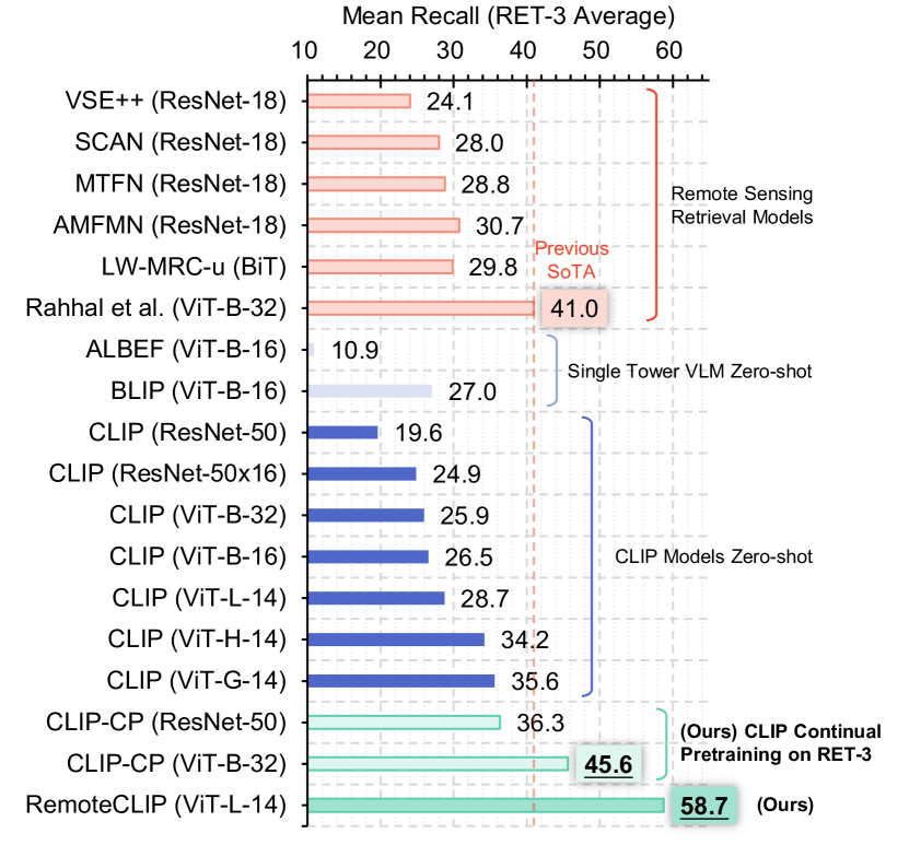
Figure 1: Averaged mean recall on three remote sensing image-text retrieval benchmarks: RSITMD, RSICD, and UCM (RET-3). Key findings: (1) Zero-shot retrieval of large CLIP models (e.g., ViT-G-14) outperforms all previous models specifically designed for remote sensing retrieval, except for the method from Rahhal et al. [47] that fine-tuned a CLIP model. (2) Simply performing continual pretraining (CLIP-CP) significantly boosts the performance of CLIP models and establishes a new SOTA model.

III-A2 Continual pretraining on small CLIP further improves the performance

Given the strong results of large CLIP models on remote sensing tasks, a natural question is whether we can further improve their performance using in-domain aerial imaginary data. Continual pretraining is a popular methodology to achieve this goal, which has already shown its advantages for adapting CLIP models into the medical domain [64]. As an initial experiment, we perform continuous pretraining of the CLIP model (ResNet-50 and ViT-Base-32) on the union of three existing retrieval datasets RSITMD, RSICD, and UCM (RET-3) . We used the standard CLIP training setup, following common practice [62, 63, 64]. The resulting models, which we denote as CLIP-CP, yield extremely powerful performance. As shown in Fig. 1, it not only outperforms the zero-shot results of the largest CLIP model (ViT-G-14) with only 2% (38M vs. 1.8B) parameters but also establishes a new state-of-the-art performance on these three retrieval benchmarks.

It is also clear that tuning the foundation model on a collection of datasets is beneficial. Compared to the model of Rahhal et al. [47] using the same ViT-Base-32 architecture, our approach – continual pretraining on the RET-3 collection – improved the performance by a clear margin (4.6%). This multi-dataset tuning shares a similar spirit with recent studies on vision language learning, such as InstructBLIP [70], PaLI-X [71], and Clever Flamingo [72].

Such a simple continuous pretraining strategy yields encouraging results, but it is still far from perfect: when we try to scale up the model size (e.g., to ViT-Large-14), a severe over-fitting phenomenon appears. The reason is quite clear – the dataset used for continuous retraining is too small for a large CLIP model. The combination of all existing image-text data (RET-3) only has 13k samples, while the pretraining data for CLIP models usually range from several hundred million to several billion samples. This motivates us to perform data scaling to match the model capacity and complexity of large CLIP models. As shown in the last row in Fig. 1, such data scaling yields impressive results (+17.7% compared to the previous SOTA results). The details of our data scaling method are presented in the following section.

III-B Data Scaling via Annotation Unification

We have already shown that the vanilla CLIP model and its continual-pretrained version are promising for vision language tasks in the remote sensing domain. We have also identified that data scale is the major bottleneck limiting performance. These observations motivate us to scale up the dataset for continuous pretraining beyond the currently available image-text pairs (RET-3 with only 13k samples). A straightforward methodology is to annotate more captions based on crowd-sourcing, but despite this being very expensive therefore significantly lowering the scalability, the annotation quality and diversity are also hard to guarantee.

To solve this issue and thereby unleash the full potential of CLIP models, here we propose to scale up the dataset via annotation unification. We find that existing datasets annotated with object bounding boxes and class names, which were originally constructed for training object detectors, provide valuable information about the semantics within each satellite image. However, such object bounding box annotation can not be directly understood by the text encoder of CLIP, as it has only been trained on natural language captions. Therefore, we propose a Box-to-Caption (B2C) generation approach to transfer the bounding box annotations into a set of natural language captions to mitigate this gap. Further, to utilize the annotation in segmentation datasets, we propose to use a Mask-to-Box (M2B) conversion method to unify segmentation datasets into bounding box annotations, and subsequently transfer them into captioning datasets. An overview of this process is shown in Fig. 2.

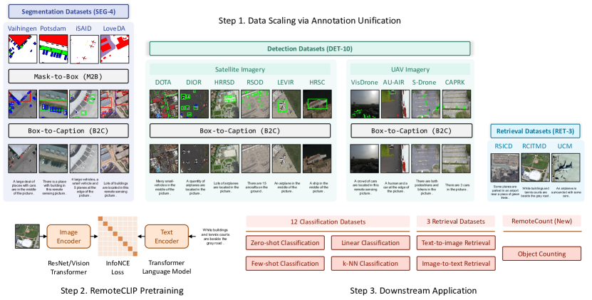
Figure 2: Overview of the RemoteCLIP pipeline. Step 1: RemoteCLIP is trained on a diverse collection of remote sensing datasets, covering 10 object detection datasets (DET-10, 6 of them are satellite imaginary datasets and 4 of them are UAV datasets), 4 remote sensing semantic segmentation datasets (SEG-4), and three remote sensing image-text datasets. We propose Box-to-Caption (B2C) generation and Mask-to-Box (M2B) conversion to fully utilize heterogeneous annotations, and scale up the training data to 12$\times$ of the combination of all involved image-text data. Step 2: We perform continual pretraining based on the CLIP model, specializing it in the remote sensing domain. Step 3: we perform a comprehensive evaluation on 7 tasks using 16 downstream datasets, including a newly created RemoteCount dataset, to demonstrate the strong capability and generalization ability of RemoteCLIP.

III-B1 Box-to-Caption (B2C) Generation

The Box-to-Caption (B2C) generation enables the generation of textual descriptions for object detection datasets based on bounding box annotations and labels. This method employs a rule-based approach to generate five distinct captions that describe the objects in the image.

Specifically, the first two captions are generated according to the target location (the center point of the bounding box): the first caption describes the objects in the center of the image, while the second one describes the objects that are not located in the center. This differentiation provides additional context and information about the spatial distribution of objects within the image.

The remaining three captions are generated by considering the number of different object categories in the image. Random objects from the list of bounding box annotations are selected, and a caption is generated accordingly. In cases where the number of appearances of an object exceeds ten, a more general term (e.g., “many”, “a lot of”) is used instead of the exact number to enhance the readability and variability of the captions.

III-B2 Mask-to-Box (M2B) Conversion

The conversion of segmentation annotations to bounding box annotations is a crucial step for the seamless integration of segmentation datasets into the B2C generation pipeline. To perform such conversion, the segmentation mask is processed by category, encoding each pixel label corresponding to the target class. Next, the contour points of the connected regions for each class in the mask image are identified. These contour points provide the necessary information to determine the bounding box coordinates. By sorting the horizontal and vertical coordinates of the contour points, we can extract the minimum and maximum values, denoted as $(x_{min}$, $y_{min})$ and $(x_{max}$, $y_{max})$, respectively. These coordinate positions define the bounding box.

The steps mentioned above can be found in Fig. 3. To enhance clarity, different colors are assigned to represent bounding boxes corresponding to distinct categories. Specifically, we utilize Suzuki’s border following algorithm  [73] for contour extraction. This algorithm defines the outer boundary and the hole boundary, and it scans the binary image from left to right to find the starting point of the outer boundary or hole boundary. By traversing the neighborhood of this starting point, the algorithm determines whether to update the pixel values based on certain rules, and ultimately extracts the hierarchical relationships among the contours. As this algorithm only supports binary images as input, we need to process segmentation masks by category. The category in need of contour extraction is identified as the foreground, while the remaining categories are treated as background.

Subsequently, we apply the border following algorithm to extract the topological structure of connected components within the binary mask. By sorting the contour points of the outer boundary for each connected component, the minimum and maximum values on the horizontal and vertical axes are considered as the coordinates for the horizontal bounding box of each connected component. As shown in Fig. 2, all the semantic segmentation annotations are converted to bounding box annotations via M2B, then B2C is performed to obtain the corresponding captions.

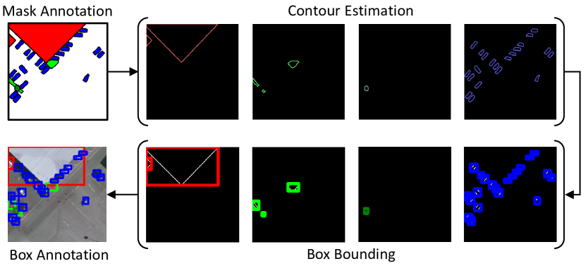
Figure 3: Mask-to-Box (M2B) implementation details. First, we get contours of per class from the input mask. Then, we select the lower left and upper right points of each contour as its bbx coordinates. Finally, we can get the bounding boxes of each category in the input mask.

III-B3 Sample De-duplication

RemoteCLIP is trained on a combination of datasets from different sources, and tested on a variety of downstream benchmarks, so it is essential to avoid possible test-set contamination. P-Hash [74] serves as a method used for image retrieval and similarity calculation by representing image features through converting the image into a fixed-length hash value. We employ p-Hash-based block-wise local detection to identify duplicate images. Specifically, we generate p-Hash values for all images and partition each value into N segments. Simultaneously, N dictionaries are established, where each dictionary’s key corresponds to the segment index, and the value comprises p-Hash values of all images in that segment. By traversing all dictionaries, we compute the Hamming distance between p-hash values of pair-wise images. If the distance between two images is less than the threshold of 2, they are considered duplicates. Upon observing the removed duplicated samples, when the threshold is set greater than 2, it is prone to excessive de-duplication. Conversely, de-duplication would be insufficient. Finally, the number of removed duplicated samples ranges from 40 to 3k in different datasets.

III-C Data Analysis

Based on the proposed B2C generation and M2B conversion method, we can efficiently translate heterogeneous annotations in various detection or segmentation datasets into image-text samples based on the pipeline shown in Fig. 2. For a deeper understanding of the dataset produced by such a scaling pipeline, in this section, we present a detailed and comprehensive analysis of this dataset. Firstly, in Table I, we provide the details of each source dataset used to expand the data, which can be divided into the following three groups:

1. Retrieval Data (RET-3). Three major image-text datasets for remote sensing, i.e., RSICD [29], RSITMD [28], UCM [30], are directly adopted. Captions of these datasets are annotated by humans, which results in high caption quality but a small dataset size.

2. Detection Data (DET-10). The detection dataset is the major source for dataset expansion. We combined six remote sensing datasets with object detection annotation, including DOTA [75], DIOR [76], HRRSD [77], RSOD [78], LEVIR [79] and HRSC [80]. As shown in Table I, these datasets have a significantly higher resolution than RET-3 datasets (at least 800$\times$600 vs. 224$\times$224). This group of datasets also exhibits high diversity as it consists of both satellite imagery and UAV imagery. The average number of objects in each image ranges from 1 (HRSC) to 70 (DOTA).

3. Segmentation Data (SEG-4). Four popular remote sensing semantic segmentation datasets, including Vaihingen [81], Postdam [82], iSAID [83], and LoveDA [84], are adopted and translated via M2B then B2C. These datasets also have high image resolution and domain diversity. Average number of objects ranges from 2 (Vaihingen) to 33 (ISAID).

TABLE I: dataset statics

	Dataset	Year	#Image	#Class	#Box	Avg. Res.	Description
RET-3	RSICD [29]	2017	8483	-	-	224×224	RSICD dataset contains more than ten thousands remote sensing images
	RSITMD [28]	2021	3603	-	-	256×256	RSITMD dataset contains multi-source remote sensing images and textual descriptions
	UCMerced [30]	2018	1676	-	-	256×256	UCMerced dataset covers 21 different scene classes, with 100 images per class.
DET-10	AUAIR [85]	2020	32,823	8	132,031	1920×1080	AU-AIR dataset features multi-modal sensor data, including visual, temporal, location, altitude, IMU, velocity, and more.
	CARPK [86]	2017	1,568	1	106,690	1280×720	CARPK dataset contains nearly 90,000 cars collected from four different parking lots by drones.
	DIOR [76]	2019	23,463	20	192,472	800×800	DIOR dataset consists of 190,288 instances of 20 different object classes, with approximately 1,200 images per class.
	DOTA [75]	2017	1,409	15	98,990	1504×1395	DOTA dataset consists of 188,282 instances of 15 different object classes, including airplanes, ships, and others.
	HRRSD [77]	2019	21,761	13	57,137	1406×1264	HRRSD dataset is used for studying object detection in high-resolution remote sensing images.
	HRSC [80]	2017	1,055	1	1,055	1105×791	HRSC dataset includes high-resolution satellite images along with corresponding ship positions and class labels.
	LEVIR [79]	2020	37.91	3	11,028	800×600	LEVIR dataset covers most types of ground features in human residential environments, such as urban, rural, and mountainous.
	RSOD [78]	2021	936	4	7,400	1051×900	RSOD dataset includes objects such as airplanes, oil tanks, sports fields, and overpasses.
	Stanford [87]	2016	17,351	6	355,443	1424×1088	Stanford Drone dataset contains trajectory and interaction information of 20,000 objects on campus in drones perspective.
	Visdrone [88]	2018	6,471	11	77,547	1509×849	Visdrone dataset consists of high-quality images and videos captured by UAV, along with rich object annotation information.
SEG-4	iSAID [83]	2019	30,821	15	987,239	896×896	iSAID dataset consists of a large number of high spatial resolution images and includes fifteen important and common categories.
	loveDA [84]	2021	4,187	6	97,989	1024×1024	LoveDA dataset consists of high-resolution images and 166,768 annotated semantic objects from 3 cities.
	Potsdam [82]	2012	5,421	4	92,161	512×512	Potsdam dataset is a semantic segmentation urban remote sensing dataset and involves five foreground classes .
	Vaihingen [81]	2012	742	4	16,875	512×512	Vaihingen dataset is also used for semantic segmentation and involves the same category information as the Potsdam dataset

In Fig. 4, we present a visualization of the caption length distribution for both the RET-3 data and our final data. It is evident from the figure that the B2C and M2B approaches yield a caption distribution that closely mirrors that of the RET-3 data. Furthermore, Fig. 5 provides visualizations of word clouds and the top 20 keywords, with common stop-words such as “there”, “an”, “is”, and others being filtered out.

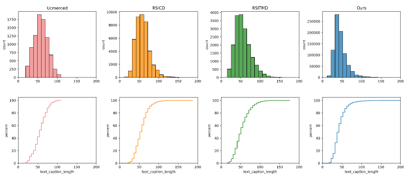
Figure 4: Distribution of caption length of existing image-text datasets UCM (pink), RSICD (yellow), RSITMD (green), and our final dataset (blue).

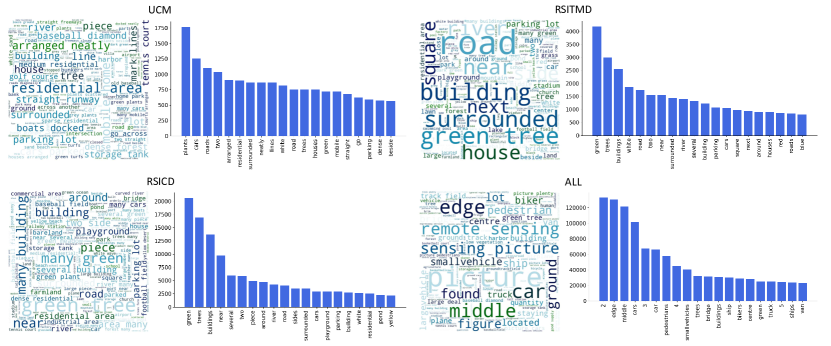
Figure 5: Word clouds and top 20 keywords of captions in existing image-text datasets UCM, RSITMD, and RSICD and our final dataset produced by B2C and M2B from DET-10, SEG-4, and RET-3.

Finally, we produce a T-SNE visualization of our final data (DET-10 + SEG-4 + Ret-3). We select 2k samples from each subset in our final data for T-SNE visualizations. For the text T-SNE visualization, we employ paraphrase-distilroberta-base-v2 from Sentence-Transformer to extract features from textual descriptions. For the image T-SNE visualization, we simply choose ViT-Base-32 from OpenCLIP to extract visual features. From Fig. 6, it can be seen that our data scaling approach provides much more enriched samples. Learning multimodal representations from such a diverse sample distribution results in a strong RemoteCLIP model that handles downstream tasks in various domains.

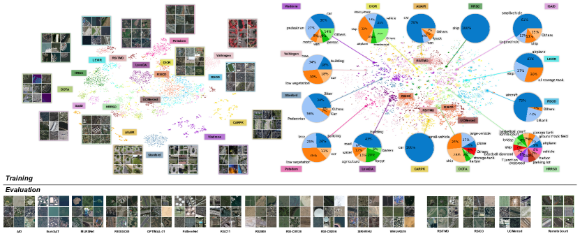
Figure 6: T-SNE visualization of image (upper left) and caption samples (upper right) in our final dataset. We provide random image samples of each dataset and label distribution of the caption samples. In the bottom row, we visualize random samples from downstream datasets used for evaluation, including 12 classification datasets, 3 retrieval datasets, and a novel object counting dataset.

IV Experiments

IV-A Implementation Details

IV-A1 Model

We select three types of visual backbone architecture for the RemoteCLIP model, ranging from a small-scale model ResNet-50 of 38M parameters, a medium-scale model ViT-Base-32 of 87M parameters to a large-scale model ViT-Large-14 of 304M parameters, to prove that our data scaling approach benefit different sizes of models. The ResNet-50 structure is modified from the OpenAI version. It replaces the original three 3×3 convolutions with a single 7×7 convolution and replaces the average pooling with the max pooling. Additionally, an anti-aliased rect-2 blur pooling layer is added on top of the ResNet-50 architecture, and the original average pooling layer is replaced with a multi-head self-attention-based pooling. ViT-B-32 partitions the input image into fixed-size image patches of 32×32 pixels and consists of 12 layers and 12 attention heads. ViT-L-14 partitions the input image into patches of 14×14 pixels and comprises 24 layers and 16 attention heads. The text encoder utilizes the Transformer architecture, consisting of 12 layers and 8 attention heads. The maximum token sequence length is set to 77, the same as the original OpenAI CLIP. The InfoNCE loss operates on the [CLS] token produced by the image and text backbone.

IV-A2 Data and preprocessing

Our final training dataset comprises a total of 165,745 images, with each image accompanied by 5 corresponding captions. This results in 828,725 training image-text pairs. For data augmentation, we utilize standard operations. For instance, we employ random crops to resize images, ensuring they align with the model’s input specifications by adjusting them to the required sizes and resolutions. To enhance dataset diversity and bolster the model’s robustness across various image orientations, we apply random horizontal flips, random rotations of 0^∘, 90^∘, 180^∘, and 270^∘ degrees to the images to encourage rotation invariance.

IV-A3 Optimization

The implementation of RemoteCLIP is based on the ITRA codebase developed from OpenCLIP. We utilize automatic mixed-precision (AMP) to maintain model accuracy while reducing memory usage. Similar to CLIP, The training process is accelerated by employing the Adam optimizer. We adopt linear warm-up and cosine learning rate scheduler. The learning rate is set to 7e-5, 4e-5, and 1e-4 respectively for ResNet-50, ViT-Base-32, and ViT-Large-14 models, and the corresponding batch size is set to 256, 256, and 28, respectively. We train all models for a total step of 108,215. Using a single-node 4$\times$NVIDIA 3090Ti machine, training our largest RemoteCLIP model takes 233.4 hours.

IV-B Benchmarking RemoteCLIP

TABLE II: Cross-modal retrieval performance on RSITMD, RSICD and UCM benchmarks. CLIP-CL corresponds to the continual pretraining of CLIP on existing RET-3 data only (details presented in Section III-A2). Previous SOTA results are marked by RED, while the RemoteCLIP models are marked by BLUE. Our RemoteCLIP achieves the SOTA performance on all three retrieval benchmarks by a large margin compared to previous approaches.

Testing Dataset	Training Dataset	Training Samples	Date	Method	Image Backbone		Text Backbone		Total Params	Image to Text			Text to Image			Mean Recall
					Name	Params	Name	Params		R@1	R@5	R@10	R@1	R@5	R@10
RSITMD	RSITMD	4,743	Jul 2017	VSE++ [89]	VGG19	-	GRU	-	-	10.38	27.65	39.60	7.79	24.87	38.67	24.83
			Mar 2018	SCAN [90]	ResNet-101	-	GRU	-	-	11.06	25.88	39.38	9.82	29.38	42.12	26.28
			Aug 2019	MTFN [91]	ResNet	-	GRU	-	-	10.40	27.65	36.28	9.96	31.37	45.84	26.92
			Aug 2020	AMFMN [92]	ResNet-50	-	GloVe fasText	-	-	10.63	24.78	41.81	11.51	34.69	54.87	29.72
			Dec 2020	LW-MRC-u [45]	Big Transfer	-	Bi-LSTM	-	-	9.73	26.77	37.61	9.25	34.07	54.03	28.58
			Apr 2022	GaLR [46]	ResNet-18	-	GRU	-	-	14.82	31.64	42.48	11.15	36.68	51.68	31.41
			Dec 2022	CMFM-Net [48]	ResNet-18	-	GRU	-	-	10.84	28.76	40.04	10.00	32.83	47.21	28.28
			Dec 2022	HyperMatch [49]	ResNet-18	-	GRU	-	-	11.73	28.10	38.05	9.16	32.31	46.64	27.66
			Oct 2022	Rahhal et al. [47]	ViT-B-32	87	Transformer	63	151	19.69	40.26	54.42	17.61	49.73	66.59	41.38
			Sept 2023	HVSA [51]	ResNet-18	-	GRU	-	-	13.20	32.08	45.58	11.43	39.20	57.45	33.16
			May 2022	FBCLM [93]	Resnet-18	-	BERT	-	-	12.84	30.53	45.89	10.44	37.01	57.94	32.44
			Oct 2023	DOVE [94]	ResNet-50	-	GRU	-	-	16.81	36.80	49.93	12.20	49.93	66.50	38.70
			Oct 2023	PIR [95]	SwinT+ ResNet-50	-	Bert	-	-	18.14	41.15	52.88	12.17	41.68	63.41	38.24
	RET-3	13,713	-	CLIP-CL	ResNet-50	38	Transformer	64	102	19.25	39.82	51.33	15.09	41.46	56.64	37.27
			-	CLIP-CL	ViT-B-32	88	Transformer	64	151	24.78	50.00	63.27	22.61	55.27	69.87	47.63
	RET-3 + DET-10 + SEG-4	165,745	Jun 2023	RemoteCLIP	ResNet-50	38	Transformer	64	102	23.67	47.57	64.60	19.29	51.55	70.58	46.21
			Jun 2023	RemoteCLIP	ViT-B-32	87	Transformer	63	151	27.88	50.66	65.71	22.17	56.46	73.41	49.38
			Jun 2023	RemoteCLIP	ViT-L-14	304	Transformer	124	428	28.76	52.43	63.94	23.76	59.51	74.73	50.52
RSICD	RSICD	10,921	Jul 2017	VSE++ [89]	VGG19	-	GRU	-	-	3.38	9.51	17.46	2.82	11.32	18.10	10.43
			Mar 2018	SCAN [90]	ResNet-101	-	GRU	-	-	5.85	12.89	19.84	3.71	16.40	26.73	14.23
			Aug 2019	MTFN [91]	ResNet	-	GRU	-	-	5.02	12.52	19.74	4.90	17.17	29.49	14.81
			Aug 2020	AMFMN [92]	ResNet-50	-	GloVe fasText	-	-	5.39	15.08	23.40	4.90	18.28	31.44	16.42
			Dec 2020	LW-MRC-u [45]	Big Transfer	-	Bi-LSTM	-	-	4.39	13.35	20.29	4.30	18.85	32.34	15.59
			Apr 2022	GaLR [46]	ResNet-18	-	GRU	-	-	6.59	19.85	31.04	4.69	19.48	32.13	18.96
			Dec 2022	CMFM-Net [48]	ResNet-18	-	GRU	-	-	5.40	18.66	28.55	5.31	18.57	30.03	17.75
			Dec 2022	HyperMatch [49]	ResNet-18	-	GRU	-	-	7.14	20.04	31.02	6.08	20.37	33.82	19.75
			Sept 2022	KCR [50]	ResNet-101	-	Transformer	-	-	5.84	22.31	36.12	4.76	18.59	27.20	19.14
			Oct 2022	Rahhal et al. [47]	ViT-B-32	87	Transformer	63	151	10.70	29.64	41.53	9.14	28.96	44.59	27.43
			Sept 2023	HVSA [51]	ResNet-18	-	GRU	-	-	7.47	20.62	32.11	5.51	21,13	34,13	16.43
			May 2022	FBCLM [93]	Resnet-18	-	BERT	-	-	13.27	27.17	37.60	13.54	38.74	56.94	31.21
			Oct 2023	DOVE [94]	ResNet-50	-	GRU	-	-	8.66	22.35	34.95	6.04	23.95	40.35	22.72
			Oct 2023	PIR [95]	SwinT + ResNet-50		Bert			9.88	27.26	39.16	6.97	24.56	38.92	24.46
	RET-3	13,713	-	CLIP-CL	ResNet-50	38	Transformer	64	102	12.99	26.35	36.32	8.56	25.60	39.16	24.83
			-	CLIP-CL	ViT-B-32	88	Transformer	64	151	17.84	35.96	50.14	13.89	35.15	50.08	33.96
	RET-3 + DET-10 + SEG-4	165,745	Jun 2023	RemoteCLIP	ResNet-50	38	Transformer	64	102	13.36	32.94	44.83	10.76	32.83	48.75	30.58
			Jun 2023	RemoteCLIP	ViT-B-32	87	Transformer	63	151	17.02	37.97	51.51	13.71	37.11	54.25	35.26
			Jun 2023	RemoteCLIP	ViT-L-14	304	Transformer	124	428	18.39	37.42	51.05	14.73	39.93	56.58	36.35
UCM	UCM	2,100	Jul 2017	VSE++ [89]	VGG19	-	GRU	-	-	12.38	44.76	65.71	10.10	31.80	56.85	36.93
			Mar 2018	SCAN [90]	ResNet-101	-	GRU	-	-	12.85	47.14	69.52	12.48	46.86	71.71	43.43
			Aug 2019	MTFN [91]	ResNet	-	GRU	-	-	10.47	47.62	64.29	14.19	52.38	78.95	44.65
			Aug 2020	AMFMN [92]	ResNet-50	-	GloVe fasText	-	-	16.67	45.71	68.57	12.86	53.24	79.43	46.08
			Dec 2020	LW-MRC-u [45]	Big Transfer	-	Bi-LSTM	-	-	18.10	47.14	63.81	13.14	50.38	79.52	45.35
			Oct 2022	Rahhal et al. [47]	ViT-B-32	87	Transformer	63	151	19.04	53.33	77.61	19.33	64.00	91.42	54.12
			May 2022	FBCLM [93]	Resnet-18	-	BERT	-	-	28.57	63.81	82.86	27.33	72.67	94.38	61.60
	RET-3	13,713	-	CLIP-CL	ResNet-50	38	Transformer	64	102	14.29	44.76	72.86	13.52	53.71	82.10	46.87
			-	CLIP-CL	ViT-B-32	88	Transformer	64	151	20.00	55.24	80.95	18.19	64.86	92.38	55.27
	RET-3 + DET-10 + SEG-4	165,745	2023	RemoteCLIP	ResNet-50	38	Transformer	64	102	13.33	50.48	74.76	15.24	57.14	84.57	49.25
			2023	RemoteCLIP	ViT-B-32	87	Transformer	63	151	20.48	59.85	83.33	18.67	61.52	94.29	56.36
			Jun 2023	RemoteCLIP	ViT-L-14	304	Transformer	124	428	19.05	54.29	80.95	17.71	62.19	93.90	54.68

IV-B1 Cross-modal Retrieval

We first present the performance of RemoteCLIP on three remote sensing image-text retrieval benchmarks (RSITMD, RSICD, UCM) and compare it with previous results. To perform cross-modal retrieval with RemoteCLIP, we extract image and text representations on the test split, perform L-2 normalization, and retrieve most similar samples based on the dot-product similarity measure. We report the retrieval recall of top-1 (R@1), top-5 (R@5), top-10 (R@10), and the mean recall of these values. We do not perform any dataset-specific fine-tuning or re-ranking to improve the results.

Table II summarizes the results. We also provide the details of each model, including training data, backbone architecture, and the number of parameters (in million), for better comparison. Our RemoteCILP model achieves SOTA performance on all three retrieval benchmarks. On the challenging RSITMD and RSICD datasets, our model outperforms the previous SOTA method (Rahhal et al. [47]) by a large margin (9.14% and 8.92% respectively). Such results are achieved with the large-scale model ViT-Large-14 with 304 parameters. When it comes to smaller models, RemoteCLIP is still competitive – the ResNet-50-based RemoteCLIP can also exceed previous SOTA methods on RSITMD and RSICD datasets. In addition, on all three retrieval benchmarks, RemoteCLIP outperforms the CLIP-CL baseline which only uses the existing RET-3 data, showing the effectiveness of RemoteCLIP data scaling.

IV-B2 Object Counting

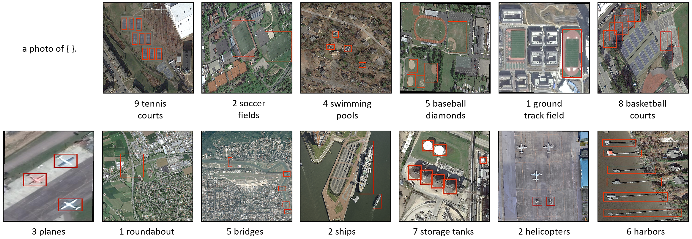
Figure 7: Visualization of the RemoteCount dataset samples. Objects of interest are annotated by red bounding boxes.

A recent study shows that large-scale pretraining empowers the CLIP model to do zero-shot object counting [96]. Here we are interested in whether RemoteCLIP has such fine-grained language understanding capability. To answer this question, we introduce a new remote sensing counting benchmark “RemoteCount” to evaluate the accuracy of object counting from 1 to 10. This dataset consists of 947 image-text pairs, which are mainly selected from the validation set of the DOTA dataset. It covers 13 categories, including planes, helicopters, roundabouts, bridges, baseball diamonds, ground track fields, basketball courts, tennis courts, harbors, soccer fields, swimming pools, ships, and storage tanks. The dataset is annotated by five graduate students, careful manual verification is conducted to ensure its quality. Fig. 7 visualize random samples within RemoteCount.

We focus on comparing the zero-shot counting accuracy of CLIP and RemoteCLIP. For each image, we augment the existing caption with nine other possible captions by replacing the number in its caption with all the numbers from 1 to 10 and calculate the similarity score between the image and each of the ten captions. The number in the caption that obtains the highest similarity score with the image is considered the predicted number.

The evaluation results are provided in Fig. 8. The top row shows the confusion matrix of CLIP and RemoteCLIP. We normalize the final output confusion matrix. CLIP has shown poor results in this task, but RemoteCLIP has a clear diagonal representing its higher accuracy. We also present the top 1 to top 10 accuracy of CLIP and RemoteCLIP. It is clear that at the top 6 accuracy level, RemoteCLIP still significantly outperforms CLIP. In addition, we also test a variation of replacing the number with “1”-“10” instead of “one”-“ten”, which we denote as “(digit)” in Fig. 8. As can be seen, RemoteCLIP is much more robust to such variation.

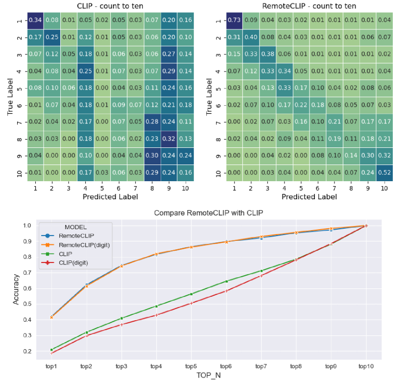
Figure 8: The object counting experiment of CLIP and RemoteCLIP on RemoteCount dataset. Upper row: The confusion matrix of CLIP and RemoteCLIP. Bottom row: Top-1 accuracy to top-10 accuracy of CLIP and RemoteCLIP.

IV-B3 Zero-shot Image Classification

TABLE III: Zero-shot accuracies on 12 remote sensing image classification datasets.

Method	Backbone	RSI-CB128	RSI-CB256	WHU-earth	EuroSAT	MLRSNet	PatternNet	RESISC45	AID	RS2800	OPTIMAL-31	RSC11	WHU-RS19	Average
CLIP	ResNet-50	26.56	34.24	40.42	42.02	45.54	46.96	53.57	57.35	62.14	64.52	64.54	69.42	50.61
RemoteCLIP		13.95	33.03	56.25	17.19	40.68	45.51	53.24	86.55	62.86	70.16	66.93	95.15	53.46
	$\pm\Delta$	-12.61	-1.21	+15.83	-24.83	-4.86	-1.45	-0.33	+29.20	+0.72	+5.64	+2.39	+25.73	+2.85
CLIP	ViT-B-32	28.88	37.35	51.18	47.11	55.29	58.95	60.92	65.65	59.31	68.62	58.35	80.61	56.02
RemoteCLIP		24.18	39.5	63.12	35.96	59.28	57.71	70.33	91.30	68.57	77.96	64.94	96.12	62.41
	$\pm\Delta$	-4.70	+2.15	+11.94	-11.15	+3.99	-1.24	+9.41	+25.65	+9.26	+9.34	+6.59	+15.51	+6.39
CLIP	ViT-L-14	40.23	47.94	58.33	60.21	64.89	73.78	69.23	69.88	72.15	76.83	67.11	87.5	65.67
RemoteCLIP		37.22	52.82	70.83	59.94	66.32	68.75	79.84	87.90	72.32	90.05	74.90	94.66	71.30
	$\pm\Delta$	-3.01	+4.88	+12.50	-0.27	+1.43	-5.03	+10.61	+18.02	+0.17	+13.22	+7.79	+7.16	+5.63

This section presents the zero-shot image classification outcome of our RemoteCLIP model. We used a total of 12 downstream datasets, including PatternNet [97], EuroSAT [98], OPTIMAL-31 [99], RSC11 [100], AID [101], MLRSNet [102], RSI-CB128 [103], RSI-CB256 [103], RESISC45 [104], WHU-earth [105], WHU-RS19 [106], and RS2800 [107]. We use the standard template-based prompting method, e.g., using “a satellite photo of {class name}.” as the text input to obtain the zero-shot classifier.

The details of evaluation results are shown in table III. It can be seen from the experimental results that it has an overall improvement compared with the CLIP baseline. Overall, RemoteCLIP improves the averaged zero-shot accuracy improvement of +2.85%, +6.39%, and +5.63% on 12 downstream datasets with three backbones, respectively. Our largest RemoteCLIP, the ViT-Large-14-based model, outperforms the CLIP counterpart on 9 out of 12 (75%) datasets.

However, the zero-shot performance of RemoteCLIP is consistently inferior to CLIP in some datasets. We suspect it is caused by the domain gap in image distribution. Our RemoteCLIP models are trained on a collection of high-resolution images (see Table I for detailed statics), but several downstream datasets, such as the EuroSAT dataset, have a much lower image resolution (e.g., 64 × 64). In addition, samples used to train RemoteCLIP usually covers rich semantics and variations, while several land cover classification datasets have a much different distribution (see visualizations in Fig. 6).

IV-B4 Few-shot Classification

Although the zero-shot classification performance of RemoteCLIP outperforms CLIP by a significant margin, in some datasets the accuracy is still far from satisfactory. In this section, we validate whether RemoteCLIP can be adapted to certain datasets with a few available training samples. We randomly sample few-shot training sets with 1, 4, 8, 16, and 32 shot samples, and use them to train an additional linear layer on top of the image representation via logistic regression. For logistic regression, the learning rate is set to 0.8, with SGD as the optimizer, and the CosineAnnealingLR scheduling strategy is used to automatically update the learning rate. We use CrossEntropyLoss as the criterion. We set the weight decay at 4e-5, the total number of epochs at 1000, and fix the batch size at 10,000. To choose suitable parameters for few-shot classification, we train the model through 5 iterations of a random search for optimal hyperparameters. Each iteration involves the use of distinct learning rates and weight decay coefficients while recording the accuracy achieved at each stage. Finally, the parameters associated with the best accuracy are used for the few-shot classification.

Fig. 9 shows the few-shot evaluation on 12 remote sensing classification datasets. We compare RemoteCLIP with a variety of baselines, including the vanilla CLIP model (ViT-Base-32 and ResNet-50), Self-supervised Learning (SSL-based) foundation visual models (SwAV, Barlow Twins, VICReg), ImageNet pretrained models (ViT-Base-32 and ResNet-50), and existing remote sensing foundation models (ViTAE and SatMAE). Visualization of experimental results shows that a few-shot training set could significantly boost the performance of RemoteCLIP models in all datasets. Using 32-shot samples, the RemoteCLIP model outperforms all compared baselines in all 12 datasets.

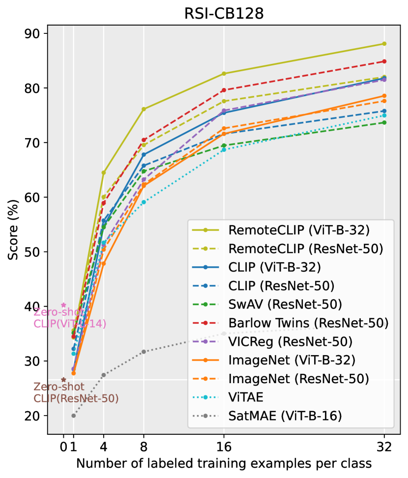
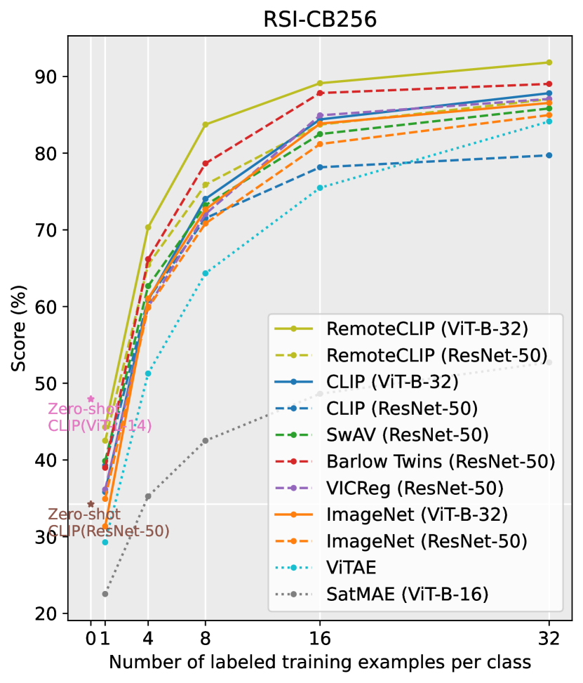
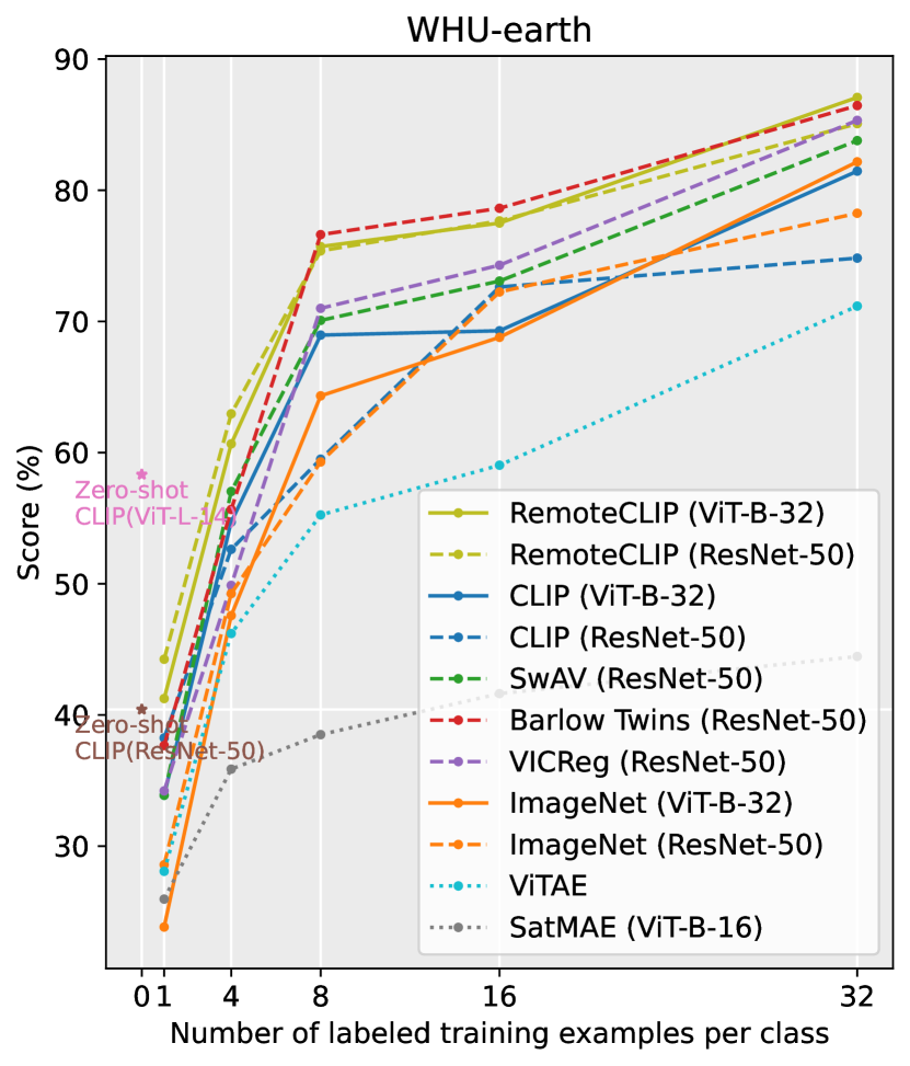
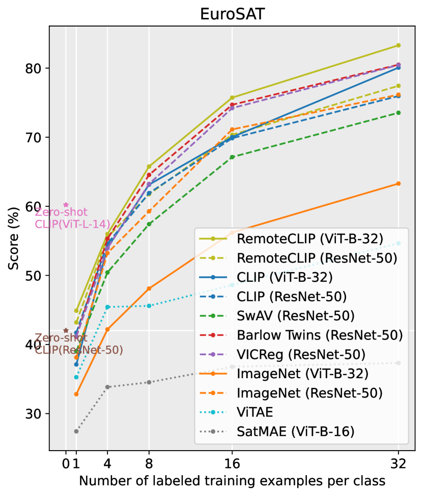
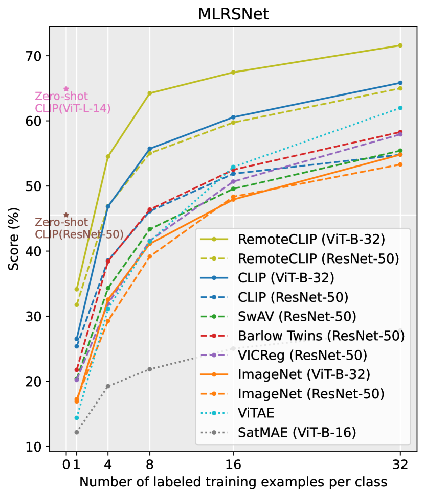
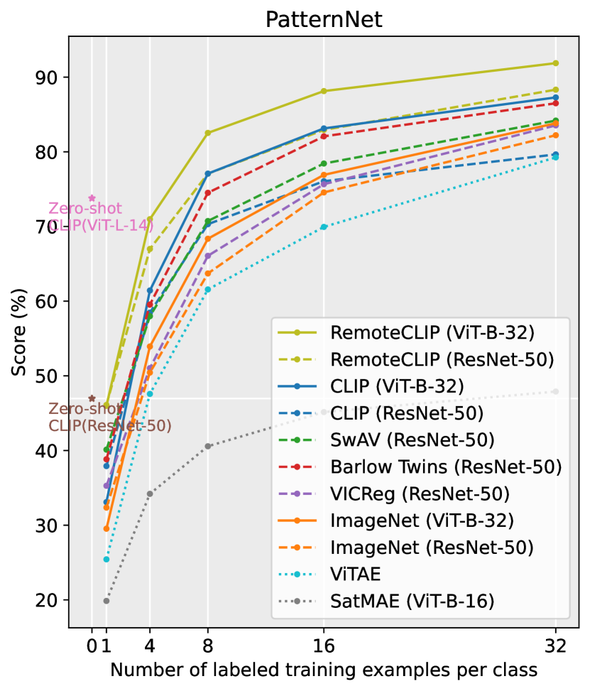
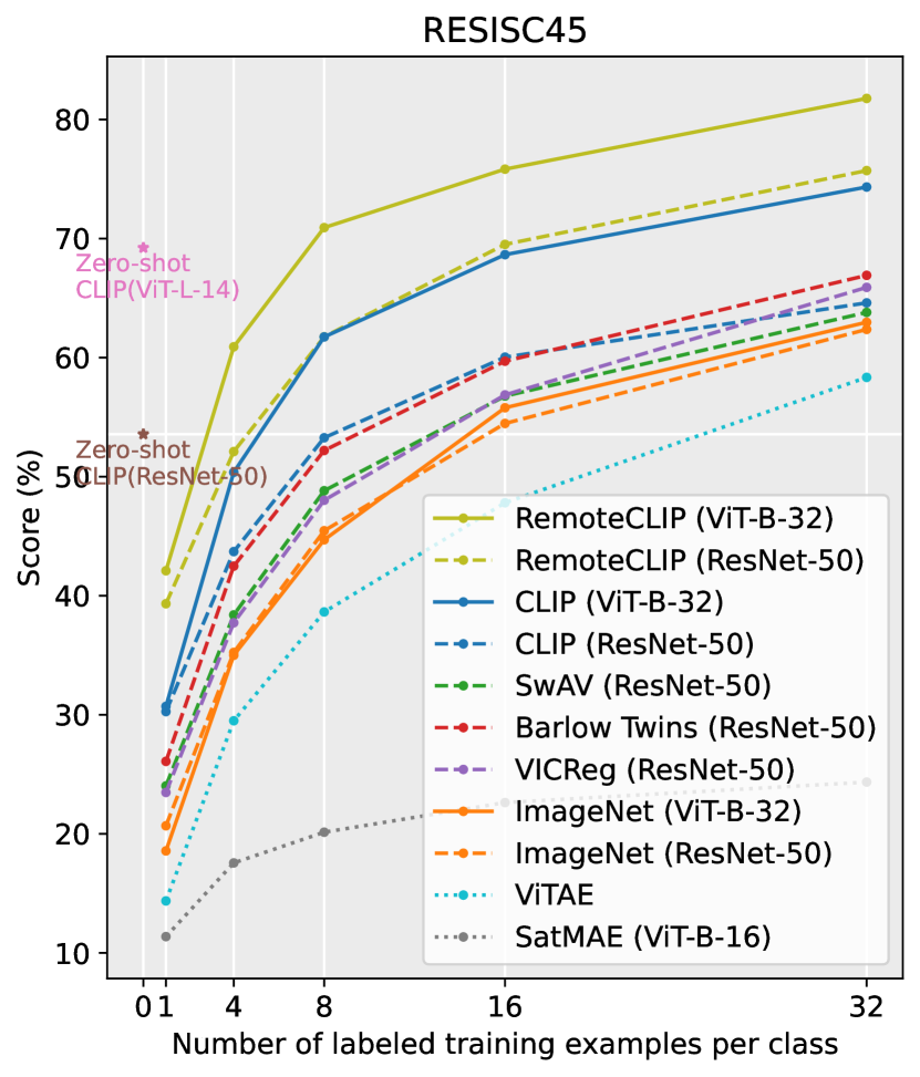
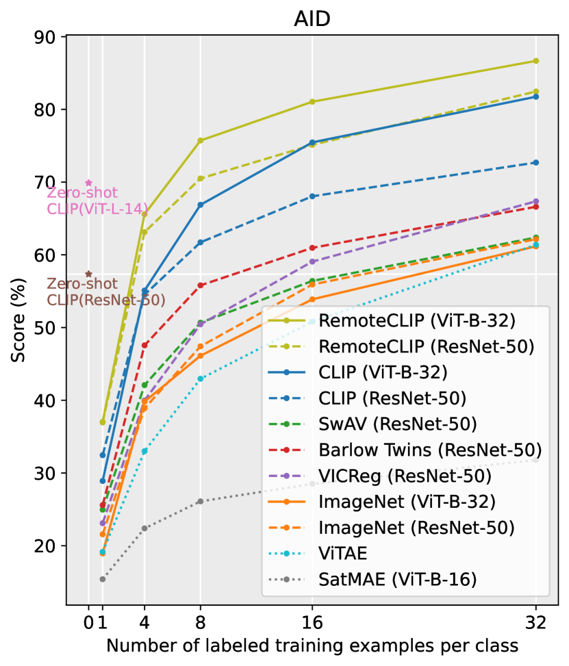
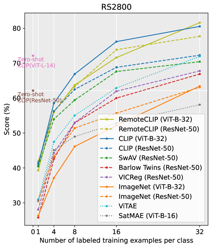
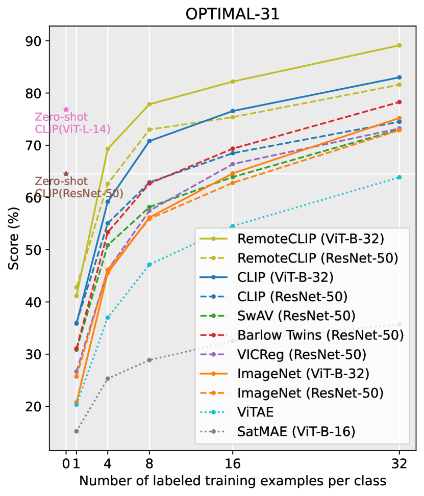
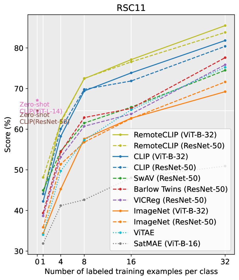
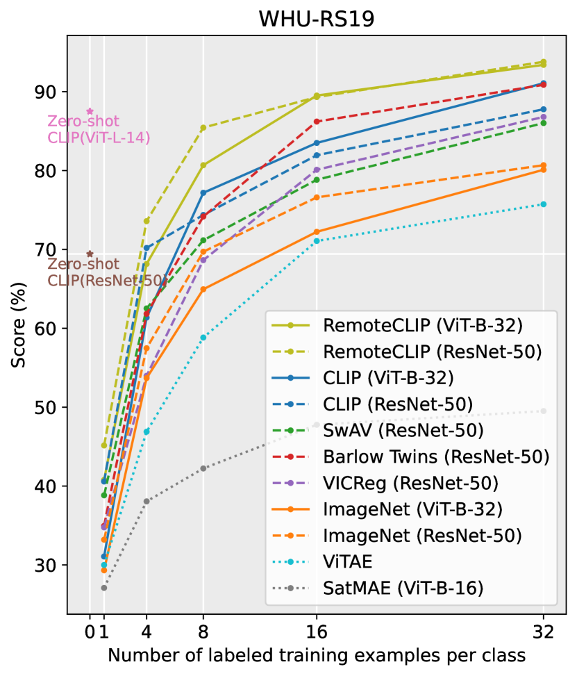
Figure 9: Few-shot classification results on 12 remote sensing datasets. Zero-shot results of CLIP models are marked by brown for ResNet-50 and by pink for ViT-L-14. On the 32-shot setting, RemoteCLIP outperforms all compared models on all 12 datasets.

IV-B5 Full-shot Linear Probing and k-NN Classification

Finally, we turn to benchmark RemoteCLIP for conventional linear probing (linear classification) and k-NN classification. We use the same 12 classification datasets previously used for zero-shot and few-shot evaluation. For linear classification, the hyperparameter settings are the same as those for the few-shot classification experiment. For k-NN classification, the number of nearest neighbors k is set to 20 and the temperature parameter T is set to 0.07. We take the accuracy of the top 1 category as the output of k-NN classification.

The results are shown in table IV. We find that the classification performance of RemoteCLIP is better than CLIP and other self-supervised models. It is not surprising that RemoteCLIP produces such strong visual representations. As mentioned in Section III-A, the vanilla CLIP model can already outperform a variety of foundation visual models in linear probing on remote sensing datasets. RemoteCLIP further enhances such representation.

TABLE IV: Linear probing and and k-NN classification results on 12 remote sensing datasets.

Method	Backbone	RSI-CB128		RSI-CB256		WHU-earth		EuroSAT		MLRSNet		PatternNet		RESISC45		AID		RS2800		OPTIMAL-31		RSC11		WHU-RS19		Average
		Linear	k-NN	Linear	k-NN	Linear	k-NN	Linear	k-NN	Linear	k-NN	Linear	k-NN	Linear	k-NN	Linear	k-NN	Linear	k-NN	Linear	k-NN	Linear	k-NN	Linear	k-NN	Linear	k-NN
ImageNet	ResNet-50	95.69	93.24	97.92	97.40	92.92	93.69	91.48	88.41	78.98	74.78	96.18	93.45	86.16	83.60	83.00	79.45	75.89	79.29	87.10	86.29	79.68	78.09	95.63	90.21	87.32	87.08
SwAV		95.27	95.61	98.59	98.17	95.20	93.96	91.17	91.37	79.04	76.12	96.94	94.18	88.60	85.59	86.00	80.80	81.07	86.07	88.44	84.14	84.86	78.89	96.12	92.23	88.97	88.83
Barlow Twins		98.07	95.91	99.03	98.13	95.83	95.42	94.78	91.57	82.41	77.55	97.73	93.83	91.10	86.10	88.25	81.75	77.32	86.07	91.94	86.83	85.26	78.09	97.09	91.75	90.00	89.73
VICReg		97.47	96.03	98.67	98.21	95.21	94.79	95.06	91.44	82.59	78.02	96.83	94.03	91.03	86.75	88.10	81.50	77.86	86.79	90.59	86.83	84.46	77.69	96.60	90.78	89.85	89.56
CLIP		94.89	94.05	97.30	97.24	93.12	91.88	91.67	88.54	80.08	77.14	95.61	92.86	85.73	85.65	90.95	86.90	83.75	81.43	88.99	87.63	87.65	87.25	97.57	93.69	89.47	89.42
CLIP-CL		95.99	94.92	98.41	98.09	96.25	94.79	89.80	87.65	79.32	76.99	97.30	95.15	89.10	88.19	94.80	92.85	82.50	89.29	91.40	89.78	91.63	84.86	98.06	97.57	91.18	91.25
RemoteCLIP		96.06	94.78	98.39	97.62	95.42	95.63	92.56	90.20	83.32	81.21	97.37	95.95	90.94	90.05	94.35	90.10	85.00	89.46	92.74	90.86	91.63	85.66	98.06	95.63	92.06	92.04
ImageNet	ViT-Base	96.45	91.29	98.11	97.00	93.75	91.67	85.57	76.56	78.61	74.05	96.81	92.98	86.89	81.63	83.55	76.45	78.93	78.04	89.51	81.18	81.67	80.88	94.17	89.81	86.34	86.05
ViTAE		93.10	95.65	98.41	94.05	93.33	78.96	61.41	82.27	91.15	80.37	98.50	90.82	87.94	65.33	88.30	64.05	92.86	78.93	86.29	54.84	92.83	71.31	91.74	70.39	84.02	83.03
CLIP		97.36	94.17	98.55	97.40	95.00	92.08	95.15	90.28	85.43	82.26	97.58	94.36	92.60	89.73	94.95	90.35	88.57	88.21	93.55	90.86	90.84	86.85	97.09	93.69	92.31	92.15
RemoteCLIP		98.02	95.82	99.01	98.51	95.42	97.08	96.19	93.50	87.00	85.11	98.47	97.32	94.27	92.67	95.95	92.55	86.96	87.86	95.97	94.35	91.63	89.24	97.57	94.17	93.93	93.77

IV-C Ablation Study

Backbone ablation: In Table V, we investigate the effects of the image and text backbones through ablation experiments conducted on the Ret-3 + Det-10 + Seg-4 dataset using RemoteCLIP. The results indicate that the optimal outcome is achieved when both the image and text backbones are pre-trained. Furthermore, the experiment highlights the greater significance of pre-training the image backbone compared to pre-training the text backbone.

Pre-training model ablation: The experimental findings can be observed in Table V. When comparing RemoteCLIP to prior pre-training techniques, notable advancements are observed in both the Retrieval task and Zero-shot tasks. Specifically, RemoteCLIP exhibits substantial improvements of approximately 10% and 15% in the Retrieval task and Zero-shot tasks, respectively.

Dataset ablation: To explore the validity of sentence-making rules, we conduct an ablation experiment on the dataset using RemoteCLIP. We apply different sentence-making rules and evaluated their impact on the same test set. The experimental results, presented in Table V, reveal superior performance with the Ret-3 + Det-10 + Seg-4 dataset. These findings indicate the task’s demand for richer textual information and affirm the effectiveness of our sentence-making strategy.

Preprocessing ablation: To ensure controlled conditions, we conduct ablation experiments on the RET-3 dataset. As shown in Table V, the retrieval results exhibit higher performance with the application of rotation.

Loss Ablation: To validate the superiority of the InfoNCE loss for RemoteCLIP, we conducted experiments comparing various loss functions. Our findings, as depicted in Table  V, demonstrate that InfoNCE effectively captures the semantic correlation between images and texts. It excels in distinguishing similarities and differences among samples, thereby leading to more robust feature representations. As a result, our experiments show that InfoNCE achieves the most favorable results, as evidenced by its superior performance across both retrieval average and zero-shot average.

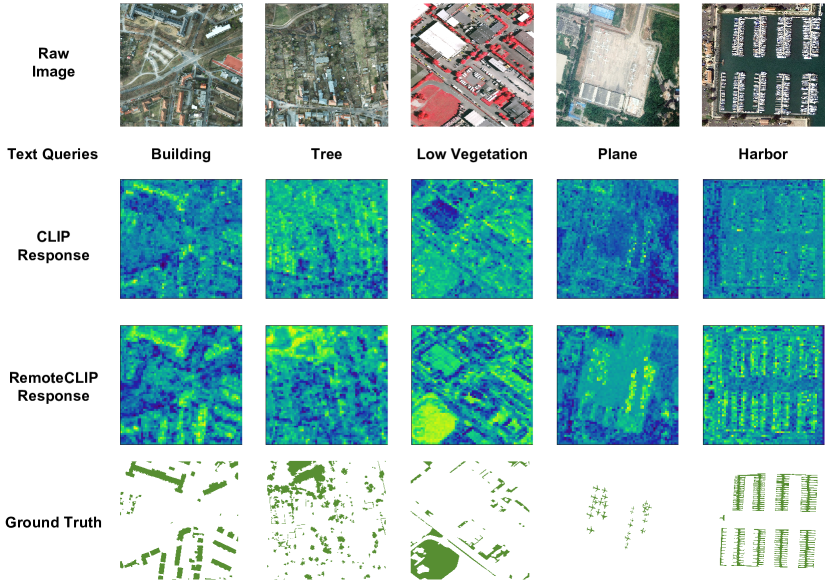
Figure 10: CLIP vs RemoteCLIP visualization of similarity across different categories. Top row: Raw images of different datasets. Above the top row are the categories for which similarity is to be calculated. Second row: Ground truth masks. For convenience, we use the same color to represent their interested category. Third row: Visualization of image-text similarity calculated by CLIP. Bottom row: Visualization of image-text similarity calculated by RemoteCLIP.

TABLE V: Ablation study results. The first row from left to right: pretraining ablation, backbone ablation and dataset ablation. The second row from left to right: preprocessing ablation and loss ablation. Settings adopted by RemoteCLIP are marked in blue.

Backbone	Method	Retrival Average	Zero-shot Average
ResNet-50	ImageNet	37.07	44.36
	SwAV	34.6	44.59
	VICReg	34.28	41.01
	BarlowTwins	32.95	40.36
	CLIP	42.01	55.06
ViT-Base	ViTAE	39.08	47.85
	ViTAE	38.75	48.5
	DINOv2	38.14	50.24
	ImageNet	35.08	46.19
	CLIP	47.00	64.52

	Image Pre-trained	Text Pre-trained	Retrival Average	Zero-shot Average
ResNet-50	✓	✓	42.01	53.46
	$\times$	✓	25.56	37.46
	✓	$\times$	35.72	46.03
	$\times$	$\times$	24.44	36.97
ViT-B-32	✓	✓	47.00	64.52
	$\times$	✓	21.56	42.60
	✓	$\times$	37.13	54.30
	$\times$	$\times$	18.92	30.93

SEG-4	DET-10	RET-3	Retrival Average	Zero-shot Average
✓	$\times$	$\times$	7.15	14.55
$\times$	✓	$\times$	9.82	21.37
$\times$	$\times$	✓	36.32	48.75
✓	✓		10.23	24.09
✓	$\times$	✓	37.24	46.94
$\times$	✓	✓	39.72	51.31
✓	✓	✓	42.01	53.46

Preprocessing	Retrival Average	Zero-shot Average
Rotation Augmentation	38.90	47.98
No Augmentation	37.74	48.05
Super Resolution	37.98	47.18
SimCLR Augmentation	37.99	48.07

Loss	Retrival Average	Zero-shot Average
InfoNCE	36.32	48.57
Margin Ranking [108]	28.93	48.47
SigLIP [109]	26.68	45.66
N-pair [110]	25.31	45.52
BarlowTwins [111]	21.03	35.44

IV-D Feature Visualization

To demonstrate that RemoteCLIP has learned richer remote sensing semantic information, we visualize the similarity scores between images and relevant categories. Specifically, we cropped high-resolution images (from Potsdam, Vaihingen, and iSAID dataset) into 64$\times$64=4096 patches with 1/3 overlap between near by patches. We employ “a {target class name}” as our text prompt, and calculate cosine similarity between patch visual feature and textual feature. We visualize the similarity score with respect to different categories in Fig. 10. Compared to that of original CLIP, the feature similarity response of RemoteCLIP has a better correlation with the ground truth mask annotation. RemoteCLIP demonstrated the ability to roughly locate the spatial position of the target category which suggests that RemoteCLIP not only learns a rich semantic information but also holds promise for tasks related to remote sensing visual localization, such as remote sensing object detection etc.

V Conclusion

In this paper, we have presented RemoteCLIP, the first general-purpose vision-language foundation model for remote sensing. During developing such a foundation model, our key insights are two-fold. First, CLIP models, which are pretrained on massive image-text pairs collected from the internet, are surprisingly powerful models for remote sensing tasks. Secondly, although in-domain fine-tuning (i.e., continual pretraining) significantly improves the performance, data quantity becomes a major bottleneck in this process, especially when we attempt to specialize large CLIP models in the remote sensing domain.

Based on the above observations, we developed a pipeline for data scaling and subsequently tune the CLIP models on the expanded dataset. The resulting RemoteCLIP model showed superior results on downstream tasks. Importantly, despite simplicity, RemoteCLIP still established a series of SOTA performances on various benchmarks. It highlights the importance of data-centric methodology in developing foundation models. Such observation is also in line with other efforts of building in-domain foundation models, such as BioMedCLIP [64] in the medical domain.

Nevertheless, RemoteCLIP still has several known limitations, and we would like to address these issues in our future works:

• Our largest RemoteCLIP model, initialized from OpenAI’s ViT-Large-14 CLIP model, boasts 304M parameters in its visual backbone and was trained on 400M data. Despite being significantly larger than previous remote sensing retrieval models, there is ample room for further scaling up. For instance, Billion-scale MAE [15] demonstrated that a ViT with a 2B scale can be successfully applied to remote sensing imagery. In the future, we plan to increase the number of model parameters to enhance the capacity of RemoteCLIP models.

• Data Scaling: Scaling up the model size necessitates a simultaneous expansion of the data scale. Although the RemoteCLIP data is already 12 times larger than the combination of all adopted image-text data in this paper, it may still be insufficient to train a much larger model. In the future, we aim to expand the pretraining data by incorporating weakly-labeled data (classification datasets) and unlabeled data (via pseudo labeling).

• Data Quality and Diversity: The quality and diversity of data are crucial. While our B2C and M2B approach effectively translates heterogeneous annotations (e.g., bounding box and segmentation maps) into homogeneous captions, our rule-based conversion methodology has limited diversity. In our future work, we plan to generate richer captions by introducing generative language models. Additionally, the modality diversity of RemoteCLIP is currently limited, and exploring more sensory modalities beyond RGB is a promising direction.

References

- [1] R. Bommasani, D. A. Hudson, E. Adeli, R. B. Altman, S. Arora, S. von Arx, M. S. Bernstein, J. Bohg, A. Bosselut, E. Brunskill, E. Brynjolfsson, S. Buch, D. Card, R. Castellon, N. S. Chatterji, A. S. Chen, K. Creel, J. Q. Davis, D. Demszky, C. Donahue, M. Doumbouya, E. Durmus, S. Ermon, J. Etchemendy, K. Ethayarajh, L. Fei-Fei, C. Finn, T. Gale, L. Gillespie, K. Goel, N. D. Goodman, S. Grossman, N. Guha, T. Hashimoto, P. Henderson, J. Hewitt, D. E. Ho, J. Hong, K. Hsu, J. Huang, T. Icard, S. Jain, D. Jurafsky, P. Kalluri, S. Karamcheti, G. Keeling, F. Khani, O. Khattab, P. W. Koh, M. S. Krass, R. Krishna, R. Kuditipudi, and et al., “On the opportunities and risks of foundation models,” CoRR, vol. abs/2108.07258, 2021. [Online]. Available: https://arxiv.org/abs/2108.07258
- [2] T. Chen, S. Kornblith, M. Norouzi, and G. E. Hinton, “A simple framework for contrastive learning of visual representations,” in Proceedings of the 37th International Conference on Machine Learning, ICML 2020, 13-18 July 2020, Virtual Event, ser. Proceedings of Machine Learning Research, vol. 119. PMLR, 2020, pp. 1597–1607. [Online]. Available: http://proceedings.mlr.press/v119/chen20j.html
- [3] K. He, X. Chen, S. Xie, Y. Li, P. Doll’ar, and R. B. Girshick, “Masked autoencoders are scalable vision learners,” 2022 IEEE/CVF Conference on Computer Vision and Pattern Recognition (CVPR), pp. 15 979–15 988, 2021.
- [4] A. Kirillov, E. Mintun, N. Ravi, H. Mao, C. Rolland, L. Gustafson, T. Xiao, S. Whitehead, A. C. Berg, W. Lo, P. Dollár, and R. B. Girshick, “Segment anything,” CoRR, vol. abs/2304.02643, 2023. [Online]. Available: https://doi.org/10.48550/arXiv.2304.02643
- [5] J. Devlin, M. Chang, K. Lee, and K. Toutanova, “BERT: pre-training of deep bidirectional transformers for language understanding,” in Proceedings of the 2019 Conference of the North American Chapter of the Association for Computational Linguistics: Human Language Technologies, NAACL-HLT 2019, Minneapolis, MN, USA, June 2-7, 2019, Volume 1 (Long and Short Papers), J. Burstein, C. Doran, and T. Solorio, Eds. Association for Computational Linguistics, 2019, pp. 4171–4186. [Online]. Available: https://doi.org/10.18653/v1/n19-1423
- [6] T. B. Brown, B. Mann, N. Ryder, M. Subbiah, J. Kaplan, P. Dhariwal, A. Neelakantan, P. Shyam, G. Sastry, A. Askell, S. Agarwal, A. Herbert-Voss, G. Krueger, T. Henighan, R. Child, A. Ramesh, D. M. Ziegler, J. Wu, C. Winter, C. Hesse, M. Chen, E. Sigler, M. Litwin, S. Gray, B. Chess, J. Clark, C. Berner, S. McCandlish, A. Radford, I. Sutskever, and D. Amodei, “Language models are few-shot learners,” in Advances in Neural Information Processing Systems 33: Annual Conference on Neural Information Processing Systems 2020, NeurIPS 2020, December 6-12, 2020, virtual, H. Larochelle, M. Ranzato, R. Hadsell, M. Balcan, and H. Lin, Eds., 2020. [Online]. Available: https://proceedings.neurips.cc/paper/2020/hash/1457c0d6bfcb4967418bfb8ac142f64a-Abstract.html
- [7] OpenAI, “Gpt-4 technical report,” ArXiv, vol. abs/2303.08774, 2023.
- [8] A. Radford, J. W. Kim, C. Hallacy, A. Ramesh, G. Goh, S. Agarwal, G. Sastry, A. Askell, P. Mishkin, J. Clark, G. Krueger, and I. Sutskever, “Learning transferable visual models from natural language supervision,” in International Conference on Machine Learning, 2021.
- [9] J. Alayrac, J. Donahue, P. Luc, A. Miech, I. Barr, Y. Hasson, K. Lenc, A. Mensch, K. Millican, M. Reynolds, R. Ring, E. Rutherford, S. Cabi, T. Han, Z. Gong, S. Samangooei, M. Monteiro, J. L. Menick, S. Borgeaud, A. Brock, A. Nematzadeh, S. Sharifzadeh, M. Binkowski, R. Barreira, O. Vinyals, A. Zisserman, and K. Simonyan, “Flamingo: a visual language model for few-shot learning,” in NeurIPS, 2022. [Online]. Available: http://papers.nips.cc/paper_files/paper/2022/hash/960a172bc7fbf0177ccccbb411a7d800-Abstract-Conference.html
- [10] H. Bao, L. Dong, S. Piao, and F. Wei, “Beit: BERT pre-training of image transformers,” in The Tenth International Conference on Learning Representations, ICLR 2022, Virtual Event, April 25-29, 2022. OpenReview.net, 2022. [Online]. Available: https://openreview.net/forum?id=p-BhZSz59o4
- [11] Z. Xie, Z. Zhang, Y. Cao, Y. Lin, J. Bao, Z. Yao, Q. Dai, and H. Hu, “Simmim: a simple framework for masked image modeling,” 2022 IEEE/CVF Conference on Computer Vision and Pattern Recognition (CVPR), pp. 9643–9653, 2021.
- [12] Y. Cong, S. Khanna, C. Meng, P. Liu, E. Rozi, Y. He, M. Burke, D. B. Lobell, and S. Ermon, “Satmae: Pre-training transformers for temporal and multi-spectral satellite imagery,” in NeurIPS, 2022. [Online]. Available: http://papers.nips.cc/paper_files/paper/2022/hash/01c561df365429f33fcd7a7faa44c985-Abstract-Conference.html
- [13] C. J. Reed, R. Gupta, S. Li, S. Brockman, C. Funk, B. Clipp, K. Keutzer, S. Candido, M. Uyttendaele, and T. Darrell, “Scale-mae: A scale-aware masked autoencoder for multiscale geospatial representation learning,” CoRR, vol. abs/2212.14532, 2022. [Online]. Available: https://doi.org/10.48550/arXiv.2212.14532
- [14] D. Wang, Q. Zhang, Y. Xu, J. Zhang, B. Du, D. Tao, and L. Zhang, “Advancing plain vision transformer toward remote sensing foundation model,” IEEE Transactions on Geoscience and Remote Sensing, vol. 61, pp. 1–15, 2022.
- [15] K. Cha, J. Seo, and T. Lee, “A billion-scale foundation model for remote sensing images,” CoRR, vol. abs/2304.05215, 2023. [Online]. Available: https://doi.org/10.48550/arXiv.2304.05215
- [16] X. Sun, P. Wang, W. Lu, Z. Zhu, X. Lu, Q. He, J. Li, X. Rong, Z. Yang, H. Chang, Q. He, G. Yang, R. Wang, J. Lu, and K. Fu, “Ringmo: A remote sensing foundation model with masked image modeling,” IEEE Transactions on Geoscience and Remote Sensing, 2022.
- [17] M. Mendieta, B. Han, X. Shi, Y. Zhu, C. Chen, and M. Li, “GFM: building geospatial foundation models via continual pretraining,” CoRR, vol. abs/2302.04476, 2023. [Online]. Available: https://doi.org/10.48550/arXiv.2302.04476
- [18] X. Kong and X. Zhang, “Understanding masked image modeling via learning occlusion invariant feature,” pp. 6241–6251, 2023. [Online]. Available: https://doi.org/10.1109/CVPR52729.2023.00604
- [19] S. Li, D. Wu, F. Wu, Z. Zang, and S. Z. Li, “Architecture-agnostic masked image modeling - from vit back to CNN,” in International Conference on Machine Learning, ICML 2023, 23-29 July 2023, Honolulu, Hawaii, USA, ser. Proceedings of Machine Learning Research, A. Krause, E. Brunskill, K. Cho, B. Engelhardt, S. Sabato, and J. Scarlett, Eds., vol. 202. PMLR, 2023, pp. 20 149–20 167. [Online]. Available: https://proceedings.mlr.press/v202/li23af.html
- [20] L. Kong, M. Q. Ma, G. Chen, E. P. Xing, Y. Chi, L. Morency, and K. Zhang, “Understanding masked autoencoders via hierarchical latent variable models,” in IEEE/CVF Conference on Computer Vision and Pattern Recognition, CVPR 2023, Vancouver, BC, Canada, June 17-24, 2023. IEEE, 2023, pp. 7918–7928. [Online]. Available: https://doi.org/10.1109/CVPR52729.2023.00765
- [21] Z. Xie, Z. Geng, J. Hu, Z. Zhang, H. Hu, and Y. Cao, “Revealing the dark secrets of masked image modeling,” in IEEE/CVF Conference on Computer Vision and Pattern Recognition, CVPR 2023, Vancouver, BC, Canada, June 17-24, 2023. IEEE, 2023, pp. 14 475–14 485. [Online]. Available: https://doi.org/10.1109/CVPR52729.2023.01391
- [22] C. Tao, X. Zhu, W. Su, G. Huang, B. Li, J. Zhou, Y. Qiao, X. Wang, and J. Dai, “Siamese image modeling for self-supervised vision representation learning,” in IEEE/CVF Conference on Computer Vision and Pattern Recognition, CVPR 2023, Vancouver, BC, Canada, June 17-24, 2023. IEEE, 2023, pp. 2132–2141. [Online]. Available: https://doi.org/10.1109/CVPR52729.2023.00212
- [23] S. Tukra, F. Hoffman, and K. Chatfield, “Improving visual representation learning through perceptual understanding,” in IEEE/CVF Conference on Computer Vision and Pattern Recognition, CVPR 2023, Vancouver, BC, Canada, June 17-24, 2023. IEEE, 2023, pp. 14 486–14 495. [Online]. Available: https://doi.org/10.1109/CVPR52729.2023.01392
- [24] N. Park, W. Kim, B. Heo, T. Kim, and S. Yun, “What do self-supervised vision transformers learn?” in The Eleventh International Conference on Learning Representations, ICLR 2023, Kigali, Rwanda, May 1-5, 2023. OpenReview.net, 2023. [Online]. Available: https://openreview.net/pdf?id=azCKuYyS74
- [25] R. Geirhos, P. Rubisch, C. Michaelis, M. Bethge, F. A. Wichmann, and W. Brendel, “Imagenet-trained cnns are biased towards texture; increasing shape bias improves accuracy and robustness,” in 7th International Conference on Learning Representations, ICLR 2019, New Orleans, LA, USA, May 6-9, 2019. OpenReview.net, 2019. [Online]. Available: https://openreview.net/forum?id=Bygh9j09KX
- [26] G. Mai, C. Cundy, K. Choi, Y. Hu, N. Lao, and S. Ermon, “Towards a foundation model for geospatial artificial intelligence (vision paper),” Proceedings of the 30th International Conference on Advances in Geographic Information Systems, 2022.
- [27] G. Mai, W. Huang, J. Sun, S. Song, D. Mishra, N. Liu, S. Gao, T. Liu, G. Cong, Y. Hu, C. Cundy, Z. Li, R. Zhu, and N. Lao, “On the opportunities and challenges of foundation models for geospatial artificial intelligence,” CoRR, vol. abs/2304.06798, 2023. [Online]. Available: https://doi.org/10.48550/arXiv.2304.06798
- [28] Z. Yuan, W. Zhang, K. Fu, X. Li, C. Deng, H. Wang, and X. Sun, “Exploring a fine-grained multiscale method for cross-modal remote sensing image retrieval,” IEEE Transactions on Geoscience and Remote Sensing, vol. 60, pp. 1–19, 2021.
- [29] X. Lu, B. Wang, X. Zheng, and X. Li, “Exploring models and data for remote sensing image caption generation,” IEEE Transactions on Geoscience and Remote Sensing, vol. 56, pp. 2183–2195, 2017.
- [30] Y. Yang and S. Newsam, “Bag-of-visual-words and spatial extensions for land-use classification,” in ACM SIGSPATIAL International Workshop on Advances in Geographic Information Systems, 2010.
- [31] Y. Wang, C. M. Albrecht, N. A. A. Braham, L. Mou, and X. X. Zhu, “Self-supervised learning in remote sensing: A review,” CoRR, vol. abs/2206.13188, 2022. [Online]. Available: https://doi.org/10.48550/arXiv.2206.13188
- [32] J. Kang, R. Fernández-Beltran, P. Duan, S. Liu, and A. J. Plaza, “Deep unsupervised embedding for remotely sensed images based on spatially augmented momentum contrast,” IEEE Transactions on Geoscience and Remote Sensing, vol. 59, pp. 2598–2610, 2020.
- [33] H. Jung, Y. Oh, S. Jeong, C. Lee, and T. Jeon, “Contrastive self-supervised learning with smoothed representation for remote sensing,” IEEE Geoscience and Remote Sensing Letters, vol. 19, pp. 1–5, 2022.
- [34] N. Jean, S. Wang, A. Samar, G. Azzari, D. B. Lobell, and S. Ermon, “Tile2vec: Unsupervised representation learning for spatially distributed data,” in The Thirty-Third AAAI Conference on Artificial Intelligence, AAAI 2019, The Thirty-First Innovative Applications of Artificial Intelligence Conference, IAAI 2019, The Ninth AAAI Symposium on Educational Advances in Artificial Intelligence, EAAI 2019, Honolulu, Hawaii, USA, January 27 - February 1, 2019. AAAI Press, 2019, pp. 3967–3974. [Online]. Available: https://doi.org/10.1609/aaai.v33i01.33013967
- [35] Z. Zhao, Z. Luo, J. Li, C. Chen, and Y. Piao, “When self-supervised learning meets scene classification: Remote sensing scene classification based on a multitask learning framework,” Remote. Sens., vol. 12, p. 3276, 2020.
- [36] W. Li, K. Chen, H. Chen, and Z. Shi, “Geographical knowledge-driven representation learning for remote sensing images,” IEEE Transactions on Geoscience and Remote Sensing, vol. PP, pp. 1–16, 2021.
- [37] V. Stojnic and V. Risojevic, “Self-supervised learning of remote sensing scene representations using contrastive multiview coding,” in IEEE Conference on Computer Vision and Pattern Recognition Workshops, CVPR Workshops 2021, virtual, June 19-25, 2021. Computer Vision Foundation / IEEE, 2021, pp. 1182–1191. [Online]. Available: https://openaccess.thecvf.com/content/CVPR2021W/EarthVision/html/Stojnic_Self-Supervised_Learning_of_Remote_Sensing_Scene_Representations_Using_Contrastive_Multiview_CVPRW_2021_paper.html
- [38] Y. Xiao, Q. Yuan, K. Jiang, J. He, Y. Wang, and L. Zhang, “From degrade to upgrade: Learning a self-supervised degradation guided adaptive network for blind remote sensing image super-resolution,” Inf. Fusion, vol. 96, pp. 297–311, 2023. [Online]. Available: https://doi.org/10.1016/j.inffus.2023.03.021
- [39] O. Mañas, A. Lacoste, X. G. i Nieto, D. Vázquez, and P. R. López, “Seasonal contrast: Unsupervised pre-training from uncurated remote sensing data,” 2021 IEEE/CVF International Conference on Computer Vision (ICCV), pp. 9394–9403, 2021.
- [40] Y. Du, Z. Liu, J. Li, and W. X. Zhao, “A survey of vision-language pre-trained models,” in International Joint Conference on Artificial Intelligence, 2022.
- [41] S. Long, F. Cao, S. C. Han, and H. Yang, “Vision-and-language pretrained models: A survey,” in Proceedings of the Thirty-First International Joint Conference on Artificial Intelligence, IJCAI 2022, Vienna, Austria, 23-29 July 2022, L. D. Raedt, Ed. ijcai.org, 2022, pp. 5530–5537. [Online]. Available: https://doi.org/10.24963/ijcai.2022/773
- [42] Z. Gan, L. Li, C. Li, L. Wang, Z. Liu, and J. Gao, “Vision-language pre-training: Basics, recent advances, and future trends,” Found. Trends Comput. Graph. Vis., vol. 14, pp. 163–352, 2022.
- [43] J. Zhang, J. Huang, S. Jin, and S. Lu, “Vision-language models for vision tasks: A survey,” CoRR, vol. abs/2304.00685, 2023. [Online]. Available: https://doi.org/10.48550/arXiv.2304.00685
- [44] T. A. M. Ali, Y. Bazi, M. M. A. Rahhal, M. L. Mekhalfi, L. Rangarajan, and M. A. A. Zuair, “Textrs: Deep bidirectional triplet network for matching text to remote sensing images,” Remote. Sens., vol. 12, p. 405, 2020.
- [45] M. M. A. Rahhal, Y. Bazi, T. Abdullah, M. L. Mekhalfi, and M. A. A. Zuair, “Deep unsupervised embedding for remote sensing image retrieval using textual cues,” Applied Sciences, 2020.
- [46] Z. Yuan, W. Zhang, C. Tian, X. Rong, Z. Zhang, H. Wang, K. Fu, and X. Sun, “Remote sensing cross-modal text-image retrieval based on global and local information,” IEEE Transactions on Geoscience and Remote Sensing, vol. 60, pp. 1–16, 2022.
- [47] M. M. A. Rahhal, Y. Bazi, N. A. Alsharif, L. Bashmal, N. A. Alajlan, and F. Melgani, “Multilanguage transformer for improved text to remote sensing image retrieval,” IEEE Journal of Selected Topics in Applied Earth Observations and Remote Sensing, vol. 15, pp. 9115–9126, 2022.
- [48] H. Yu, F. Yao, W. Lu, N. Liu, P. Li, H. You, and X. Sun, “Text-image matching for cross-modal remote sensing image retrieval via graph neural network,” IEEE J. Sel. Top. Appl. Earth Obs. Remote. Sens., vol. 16, pp. 812–824, 2023. [Online]. Available: https://doi.org/10.1109/JSTARS.2022.3231851
- [49] F. Yao, X. Sun, N. Liu, C. Tian, L. Xu, L. Hu, and C. Ding, “Hypergraph-enhanced textual-visual matching network for cross-modal remote sensing image retrieval via dynamic hypergraph learning,” IEEE J. Sel. Top. Appl. Earth Obs. Remote. Sens., vol. 16, pp. 688–701, 2023. [Online]. Available: https://doi.org/10.1109/JSTARS.2022.3226325
- [50] L. Mi, S. Li, C. Chappuis, and D. Tuia, “Knowledge-aware cross-modal text-image retrieval for remote sensing images,” in Proceedings of the Second Workshop on Complex Data Challenges in Earth Observation (CDCEO 2022) co-located with 31st International Joint Conference on Artificial Intelligence and the 25th European Conference on Artificial Intelligence (IJCAI-ECAI 2022), Vienna, Austria, July 25th, 2022, ser. CEUR Workshop Proceedings, A. Gruca, C. Robinson, N. Yokoya, J. Zhou, and P. Ghamisi, Eds., vol. 3207. CEUR-WS.org, 2022, pp. 14–20. [Online]. Available: https://ceur-ws.org/Vol-3207/paper4.pdf
- [51] W. Zhang, J. Li, S. Li, J. Chen, W. Zhang, X. Gao, and X. Sun, “Hypersphere-based remote sensing cross-modal text-image retrieval via curriculum learning,” IEEE Trans. Geosci. Remote. Sens., vol. 61, pp. 1–15, 2023. [Online]. Available: https://doi.org/10.1109/TGRS.2023.3318227
- [52] C. Jia, Y. Yang, Y. Xia, Y.-T. Chen, Z. Parekh, H. Pham, Q. V. Le, Y.-H. Sung, Z. Li, and T. Duerig, “Scaling up visual and vision-language representation learning with noisy text supervision,” in International Conference on Machine Learning, 2021.
- [53] M. Cherti, R. Beaumont, R. Wightman, M. Wortsman, G. Ilharco, C. Gordon, C. Schuhmann, L. Schmidt, and J. Jitsev, “Reproducible scaling laws for contrastive language-image learning,” ArXiv, vol. abs/2212.07143, 2022.
- [54] N. Mu, A. Kirillov, D. Wagner, and S. Xie, “Slip: Self-supervision meets language-image pre-training,” in European Conference on Computer Vision. Springer, 2022, pp. 529–544.
- [55] Y. Li, F. Liang, L. Zhao, Y. Cui, W. Ouyang, J. Shao, F. Yu, and J. Yan, “Supervision exists everywhere: A data efficient contrastive language-image pre-training paradigm,” in The Tenth International Conference on Learning Representations, ICLR 2022, Virtual Event, April 25-29, 2022. OpenReview.net, 2022. [Online]. Available: https://openreview.net/forum?id=zq1iJkNk3uN
- [56] J. Yu, Z. Wang, V. Vasudevan, L. Yeung, M. Seyedhosseini, and Y. Wu, “Coca: Contrastive captioners are image-text foundation models,” Trans. Mach. Learn. Res., vol. 2022, 2022. [Online]. Available: https://openreview.net/forum?id=Ee277P3AYC
- [57] Y. Li, H. Fan, R. Hu, C. Feichtenhofer, and K. He, “Scaling language-image pre-training via masking,” ArXiv, vol. abs/2212.00794, 2022.
- [58] D. Chen, Z. Wu, F. Liu, Z. Yang, Y. Huang, Y. Bao, and E. Zhou, “Prototypical contrastive language image pretraining,” CoRR, vol. abs/2206.10996, 2022. [Online]. Available: https://doi.org/10.48550/arXiv.2206.10996
- [59] K. Zhou, J. Yang, C. C. Loy, and Z. Liu, “Learning to prompt for vision-language models,” International Journal of Computer Vision, vol. 130, pp. 2337 – 2348, 2021.
- [60] F. Liu, T. Zhang, W. Dai, W. Cai, X. Zhou, and D. Chen, “Few-shot adaptation of multi-modal foundation models: A survey,” 2024.
- [61] Y. Zhang, H. Jiang, Y. Miura, C. D. Manning, and C. P. Langlotz, “Contrastive learning of medical visual representations from paired images and text,” in Proceedings of the Machine Learning for Healthcare Conference, MLHC 2022, 5-6 August 2022, Durham, NC, USA, ser. Proceedings of Machine Learning Research, Z. C. Lipton, R. Ranganath, M. P. Sendak, M. W. Sjoding, and S. Yeung, Eds., vol. 182. PMLR, 2022, pp. 2–25. [Online]. Available: https://proceedings.mlr.press/v182/zhang22a.html
- [62] S. Eslami, G. de Melo, and C. Meinel, “Does CLIP benefit visual question answering in the medical domain as much as it does in the general domain?” CoRR, vol. abs/2112.13906, 2021. [Online]. Available: https://arxiv.org/abs/2112.13906
- [63] Z. Wang, Z. Wu, D. Agarwal, and J. Sun, “Medclip: Contrastive learning from unpaired medical images and text,” in Proceedings of the 2022 Conference on Empirical Methods in Natural Language Processing, EMNLP 2022, Abu Dhabi, United Arab Emirates, December 7-11, 2022, Y. Goldberg, Z. Kozareva, and Y. Zhang, Eds. Association for Computational Linguistics, 2022, pp. 3876–3887. [Online]. Available: https://aclanthology.org/2022.emnlp-main.256
- [64] S. Zhang, Y. Xu, N. Usuyama, J. Bagga, R. Tinn, S. Preston, R. Rao, M. Wei, N. Valluri, C. Wong, M. P. Lungren, T. Naumann, and H. Poon, “Large-scale domain-specific pretraining for biomedical vision-language processing,” CoRR, vol. abs/2303.00915, 2023. [Online]. Available: https://doi.org/10.48550/arXiv.2303.00915
- [65] X. Dong, X. Zhan, Y. Wu, Y. Wei, M. C. Kampffmeyer, X. Wei, M. Lu, Y. Wang, and X. Liang, “M5product: Self-harmonized contrastive learning for e-commercial multi-modal pretraining,” 2022 IEEE/CVF Conference on Computer Vision and Pattern Recognition (CVPR), pp. 21 220–21 230, 2021.
- [66] F. Liu, D. Chen, X. Du, R. Gao, and F. Xu, “Mep-3m: A large-scale multi-modal e-commerce product dataset,” Pattern Recognition, 2023.
- [67] W. Shin, J. Park, T. Woo, Y. Cho, K. Oh, and H. Song, “e-clip: Large-scale vision-language representation learning in e-commerce,” Proceedings of the 31st ACM International Conference on Information & Knowledge Management, 2022.
- [68] Z. Zhang, T. Zhao, Y. Guo, and J. Yin, “RS5M: A large scale vision-language dataset for remote sensing vision-language foundation model,” CoRR, vol. abs/2306.11300, 2023. [Online]. Available: https://doi.org/10.48550/arXiv.2306.11300
- [69] J. Roberts, K. Han, and S. Albanie, “SATIN: A multi-task metadataset for classifying satellite imagery using vision-language models,” CoRR, vol. abs/2304.11619, 2023. [Online]. Available: https://doi.org/10.48550/arXiv.2304.11619
- [70] W. Dai, J. Li, D. Li, A. M. H. Tiong, J. Zhao, W. Wang, B. Li, P. Fung, and S. C. H. Hoi, “Instructblip: Towards general-purpose vision-language models with instruction tuning,” CoRR, vol. abs/2305.06500, 2023. [Online]. Available: https://doi.org/10.48550/arXiv.2305.06500
- [71] X. Chen, J. Djolonga, P. Padlewski, B. Mustafa, S. Changpinyo, J. Wu, C. R. Ruiz, S. Goodman, X. Wang, Y. Tay, S. Shakeri, M. Dehghani, D. Salz, M. Lucic, M. Tschannen, A. Nagrani, H. Hu, M. Joshi, B. Pang, C. Montgomery, P. Pietrzyk, M. Ritter, A. J. Piergiovanni, M. Minderer, F. Pavetic, A. Waters, G. Li, I. Alabdulmohsin, L. Beyer, J. Amelot, K. Lee, A. P. Steiner, Y. Li, D. Keysers, A. Arnab, Y. Xu, K. Rong, A. Kolesnikov, M. Seyedhosseini, A. Angelova, X. Zhai, N. Houlsby, and R. Soricut, “Pali-x: On scaling up a multilingual vision and language model,” CoRR, vol. abs/2305.18565, 2023. [Online]. Available: https://doi.org/10.48550/arXiv.2305.18565
- [72] D. Chen, J. Liu, W. Dai, and B. Wang, “Visual instruction tuning with polite flamingo,” CoRR, vol. abs/2307.01003, 2023. [Online]. Available: https://doi.org/10.48550/arXiv.2307.01003
- [73] S. Suzuki and K. Abe, “Topological structural analysis of digitized binary images by border following,” Comput. Vis. Graph. Image Process., vol. 30, no. 1, pp. 32–46, 1985. [Online]. Available: https://doi.org/10.1016/0734-189X(85)90016-7
- [74] C. Zauner, “Implementation and benchmarking of perceptual image hash functions,” 2010.
- [75] G.-S. Xia, X. Bai, J. Ding, Z. Zhu, S. J. Belongie, J. Luo, M. Datcu, M. Pelillo, and L. Zhang, “Dota: A large-scale dataset for object detection in aerial images,” 2018 IEEE/CVF Conference on Computer Vision and Pattern Recognition, pp. 3974–3983, 2017.
- [76] K. Li, G. Wan, G. Cheng, L. Meng, and J. Han, “Object detection in optical remote sensing images: A survey and A new benchmark,” CoRR, vol. abs/1909.00133, 2019. [Online]. Available: http://arxiv.org/abs/1909.00133
- [77] Y. Zhang, Y. Yuan, Y. Feng, and X. Lu, “Hierarchical and robust convolutional neural network for very high-resolution remote sensing object detection,” IEEE Transactions on Geoscience and Remote Sensing, vol. 57, pp. 5535–5548, 2019.
- [78] W. Sun, L. Dai, X. Zhang, P. Chang, and X. He, “Rsod: Real-time small object detection algorithm in uav-based traffic monitoring,” Applied Intelligence, vol. 52, pp. 8448 – 8463, 2021.
- [79] H. Chen and Z. Shi, “A spatial-temporal attention-based method and a new dataset for remote sensing image change detection,” Remote. Sens., vol. 12, p. 1662, 2020.
- [80] Z. Liu, L. Yuan, L. Weng, and Y. Yang, “A high resolution optical satellite image dataset for ship recognition and some new baselines,” in International Conference on Pattern Recognition Applications and Methods, 2017.
- [81] “Vaihingen dataset,” https://www.isprs.org/education/benchmarks/UrbanSemLab/2d-sem-label-vaihingen.aspx, 2012.
- [82] “Potsdam dataset,” https://www.isprs.org/education/benchmarks/UrbanSemLab/2d-sem-label-potsdam.aspx, 2012.
- [83] S. W. Zamir, A. Arora, A. Gupta, S. H. Khan, G. Sun, F. S. Khan, F. Zhu, L. Shao, G. Xia, and X. Bai, “isaid: A large-scale dataset for instance segmentation in aerial images,” in CVPR Workshops, 2019.
- [84] J. Wang, Z. Zheng, A. Ma, X. Lu, and Y. Zhong, “Loveda: A remote sensing land-cover dataset for domain adaptive semantic segmentation,” in Proceedings of the Neural Information Processing Systems Track on Datasets and Benchmarks 1, NeurIPS Datasets and Benchmarks 2021, December 2021, virtual, J. Vanschoren and S. Yeung, Eds., 2021. [Online]. Available: https://datasets-benchmarks-proceedings.neurips.cc/paper/2021/hash/4e732ced3463d06de0ca9a15b6153677-Abstract-round2.html
- [85] S. Vujasinovi’c, S. Becker, T. Breuer, S. Bullinger, N. Scherer-Negenborn, and M. Arens, “Integration of the 3d environment for uav onboard visual object tracking,” Applied Sciences, 2020.
- [86] M.-R. Hsieh, Y.-L. Lin, and W. H. Hsu, “Drone-based object counting by spatially regularized regional proposal network,” 2017 IEEE International Conference on Computer Vision (ICCV), pp. 4165–4173, 2017.
- [87] A. Robicquet, A. Sadeghian, A. Alahi, and S. Savarese, “Learning social etiquette: Human trajectory understanding in crowded scenes,” in European Conference on Computer Vision, 2016.
- [88] P. Zhu, L. Wen, X. Bian, H. Ling, and Q. Hu, “Vision meets drones: A challenge,” CoRR, vol. abs/1804.07437, 2018. [Online]. Available: http://arxiv.org/abs/1804.07437
- [89] F. Faghri, D. J. Fleet, J. R. Kiros, and S. Fidler, “Vse++: Improving visual-semantic embeddings with hard negatives,” in British Machine Vision Conference, 2017.
- [90] K. Lee, X. Chen, G. Hua, H. Hu, and X. He, “Stacked cross attention for image-text matching,” in Computer Vision - ECCV 2018 - 15th European Conference, Munich, Germany, September 8-14, 2018, Proceedings, Part IV, ser. Lecture Notes in Computer Science, V. Ferrari, M. Hebert, C. Sminchisescu, and Y. Weiss, Eds., vol. 11208. Springer, 2018, pp. 212–228. [Online]. Available: https://doi.org/10.1007/978-3-030-01225-0_13
- [91] T. Wang, X. Xu, Y. Yang, A. Hanjalic, H. T. Shen, and J. Song, “Matching images and text with multi-modal tensor fusion and re-ranking,” Proceedings of the 27th ACM International Conference on Multimedia, 2019.
- [92] G. Hoxha, F. Melgani, and B. Demir, “Toward remote sensing image retrieval under a deep image captioning perspective,” IEEE Journal of Selected Topics in Applied Earth Observations and Remote Sensing, vol. 13, pp. 4462–4475, 2020.
- [93] H. Li, W. Xiong, Y. Cui, and Z. Xiong, “A fusion-based contrastive learning model for cross-modal remote sensing retrieval,” International Journal of Remote Sensing, vol. 43, pp. 3359 – 3386, 2022. [Online]. Available: https://api.semanticscholar.org/CorpusID:250190767
- [94] Q. Ma, J. Pan, and C. Bai, “Direction-oriented visual-semantic embedding model for remote sensing image-text retrieval,” CoRR, vol. abs/2310.08276, 2023. [Online]. Available: https://doi.org/10.48550/arXiv.2310.08276
- [95] J. Pan, Q. Ma, and C. Bai, “A prior instruction representation framework for remote sensing image-text retrieval,” in Proceedings of the 31st ACM International Conference on Multimedia, MM 2023, Ottawa, ON, Canada, 29 October 2023- 3 November 2023, A. El-Saddik, T. Mei, R. Cucchiara, M. Bertini, D. P. T. Vallejo, P. K. Atrey, and M. S. Hossain, Eds. ACM, 2023, pp. 611–620. [Online]. Available: https://doi.org/10.1145/3581783.3612374
- [96] R. Paiss, A. Ephrat, O. Tov, S. Zada, I. Mosseri, M. Irani, and T. Dekel, “Teaching CLIP to count to ten,” CoRR, vol. abs/2302.12066, 2023. [Online]. Available: https://doi.org/10.48550/arXiv.2302.12066
- [97] W. Zhou, S. Newsam, C. Li, and Z. Shao, “Patternnet: A benchmark dataset for performance evaluation of remote sensing image retrieval,” ArXiv, vol. abs/1706.03424, 2017.
- [98] P. Helber, B. Bischke, A. R. Dengel, and D. Borth, “Eurosat: A novel dataset and deep learning benchmark for land use and land cover classification,” IEEE Journal of Selected Topics in Applied Earth Observations and Remote Sensing, vol. 12, pp. 2217–2226, 2017.
- [99] Q. Wang, S. Liu, J. Chanussot, and X. Li, “Scene classification with recurrent attention of vhr remote sensing images,” IEEE Transactions on Geoscience and Remote Sensing, vol. 57, pp. 1155–1167, 2019.
- [100] L. Zhao, P. Tang, and L. Huo, “Feature significance-based multibag-of-visual-words model for remote sensing image scene classification,” Journal of Applied Remote Sensing, vol. 10, 2016.
- [101] G.-S. Xia, J. Hu, F. Hu, B. Shi, X. Bai, Y. Zhong, L. Zhang, and X. Lu, “Aid: A benchmark data set for performance evaluation of aerial scene classification,” IEEE Transactions on Geoscience and Remote Sensing, vol. 55, pp. 3965–3981, 2016.
- [102] X. Qi, P. Zhu, Y. Wang, L. Zhang, J. Peng, M. Wu, J. Chen, X. Zhao, N. Zang, and P. T. Mathiopoulos, “Mlrsnet: A multi-label high spatial resolution remote sensing dataset for semantic scene understanding,” CoRR, vol. abs/2010.00243, 2020. [Online]. Available: https://arxiv.org/abs/2010.00243
- [103] H. Li, C. Tao, Z. Wu, J. Chen, J. Gong, and M. Deng, “Rsi-cb: A large-scale remote sensing image classification benchmark using crowdsourced data,” Sensors (Basel, Switzerland), vol. 20, 2017.
- [104] G. Cheng, J. Han, and X. Lu, “Remote sensing image scene classification: Benchmark and state of the art,” Proceedings of the IEEE, vol. 105, pp. 1865–1883, 2017.
- [105] B. Zhao, Y. Zhong, G.-S. Xia, and L. Zhang, “Dirichlet-derived multiple topic scene classification model for high spatial resolution remote sensing imagery,” IEEE Transactions on Geoscience and Remote Sensing, vol. 54, pp. 2108–2123, 2016.
- [106] G.-S. Xia, W. Yang, J. Delon, Y. Gousseau, H. Sun, and H. Maître, “Structural high-resolution satellite image indexing,” 2010.
- [107] Q. Zou, L. Ni, T. Zhang, and Q. Wang, “Deep learning based feature selection for remote sensing scene classification,” IEEE Geoscience and Remote Sensing Letters, vol. 12, pp. 2321–2325, 2015.
- [108] Z. Cao, T. Qin, T. Liu, M. Tsai, and H. Li, “Learning to rank: from pairwise approach to listwise approach,” in Machine Learning, Proceedings of the Twenty-Fourth International Conference (ICML 2007), Corvallis, Oregon, USA, June 20-24, 2007, ser. ACM International Conference Proceeding Series, Z. Ghahramani, Ed., vol. 227. ACM, 2007, pp. 129–136. [Online]. Available: https://doi.org/10.1145/1273496.1273513
- [109] X. Zhai, B. Mustafa, A. Kolesnikov, and L. Beyer, “Sigmoid loss for language image pre-training,” CoRR, vol. abs/2303.15343, 2023. [Online]. Available: https://doi.org/10.48550/arXiv.2303.15343
- [110] K. Sohn, “Improved deep metric learning with multi-class n-pair loss objective,” in Advances in Neural Information Processing Systems 29: Annual Conference on Neural Information Processing Systems 2016, December 5-10, 2016, Barcelona, Spain, D. D. Lee, M. Sugiyama, U. von Luxburg, I. Guyon, and R. Garnett, Eds., 2016, pp. 1849–1857. [Online]. Available: https://proceedings.neurips.cc/paper/2016/hash/6b180037abbebea991d8b1232f8a8ca9-Abstract.html
- [111] J. Zbontar, L. Jing, I. Misra, Y. LeCun, and S. Deny, “Barlow twins: Self-supervised learning via redundancy reduction,” in Proceedings of the 38th International Conference on Machine Learning, ICML 2021, 18-24 July 2021, Virtual Event, ser. Proceedings of Machine Learning Research, M. Meila and T. Zhang, Eds., vol. 139. PMLR, 2021, pp. 12 310–12 320. [Online]. Available: http://proceedings.mlr.press/v139/zbontar21a.html